lectures on a method in the theory of exponential sumspubl/ln/tifr80.pdf · exponential sums...
TRANSCRIPT

Lectures onA Method in the Theory of Exponential Sums
By
M. Jutila
Tata Institute of Fundamental ResearchBombay
1987
Lectures onA Method in the Theory of Exponential Sums
By
M. Jutila
Published for the
Tata Institute of Fundamental Research, BombaySpringer-Verlag
Berlin Heidelberg New York Tokyo1987
Author
M. JutilaDepartment of Mathematics
University of TurkuSF–20500 Turku 50
Finland
c© Tata Institute of Fundamental Research, 1987
ISBN 3–540–18366–3 Springer-Verlag Berlin. Heidelberg. New York. TokyoISBN 0–387–18366–3 Springer-Verlag New York Heidelberg. Berlin. Tokyo
No part of this book may be reproduced in anyform by print, microfilm or any other means with-out written permission from the Tata Institute ofFundamental Research, Bombay 400 005
Printed by INSDOC Regional Centre, Indian In-stitute of Science Campus, Bangalore 560 012 andpublished by H. Goetze, Springer-Verlag, Heidel-berg, West Germany
Printed In India
Preface
These lectures were given at the Tata Institute of Fundamental Researchin October - November 1985. It was my first object to present a self-contained introduction to summation and transformation formulae forexponential sums involving either the divisor functiond(n) or the Fouriercoefficients of a cusp form; these two cases are in fact closely analogous.Secondly, I wished to show how these formulae - in combination withsome standard methods of analytic number theory - can be applied tothe estimation of the exponential sums in question.
I would like to thank Professor K. Ramachandra, Professor R.Bala-subramanian, Professor S. Raghavan, Professor T.N. Shorey, and Dr. S.Srinivasan for their kind hospitality, and my whole audience for interestand stimulating discussions. In addition, I am grateful to my colleaguesD.R. Heath-Brown, M.N. Huxley, A. Ivic, T. Meurman, Y. Motohashi,and many others for valuable remarks concerning the presentnotes andmy earlier work on these topics.
iv
Notation
The following notation, mostly standard, will occur repeatedly in thesenotes.
γ Euler’s constant.s = σ + it, a complex variable.ζ(s) Riemann’s zeta-function.Γ(s) The gamma-function.χ(s) = 2sπs−1Γ(1− s) sin(πs/2).Jn(z),Yn(z),Kn(z) Bessel functions.e(α) = e2πiα.ek(α) = e2πiα/k.Res(f ,a) The residue of the functionf at the pointa.∫
(c)
f (s) ds The integral of the functionf over the line Res= c.
d(n) The number of positive divisors of the integern.a(n) Fourier coefficient of a cusp form.
ϕ(s) =∞∑
n=1a(n)n−s.
κ The weight of a cusp form.a(n) = a(n)n−(κ−1)/2.r = h/k, a rational number with (h, k) = 1 andk ≥ 1.h The residue (modk) defined byhh ≡ 1 (modk).
E(s, r) =∞∑
n=1d(n)e(nr)n−s.
ϕ(s, r) =∞∑
n=1a(n)e(nr)n−s.
‖ α ‖ The distance ofα from the nearest integer.∑′
n≦x
f (n) =∑
1≦n≦xf (n), except that ifx is an integer,
then the termf (x) is to be replaced by12 f (x).∑′
a≦n≦b
f (n) A sum with similar conventions as above
if a or b is an integer.
v
vi Notation
D(x) =∑′
n≦x
d(n).
A(x) =∑′
n≦x
a(n).
D(x, α) =∑′
n≦x
d(n)e(nα).
A(, α) =∑′
n≦x
a(n)e(nα).
Da(x) = 1a!
∑′
n≦x
d(n) (x− n)a.
Aa(x),Da(x, α),Aa(x, α) are analogously defined.ǫ An arbitrarily small positive constant.A A constant, not necessarily the same at
each occurrence.Cn[a,b] The class of functions having a continuous
nth derivative in the interval [a,b].
The symbols 0(),≪, and≫ are used in their standard meaning.Also, f ≍ g means thatf andg are of equal order of magnitude, i.e. that1≪ f /g≪ 1. The constants implied by these notations depend at moston∈.
Contents
Preface iv
Notation v
Introduction 1
1 Summation Formulae 71.1 The FunctionE(s, r) . . . . . . . . . . . . . . . . . . . 81.2 The Functionϕ(s, r) . . . . . . . . . . . . . . . . . . . . 121.3 Aysmptotic Formula . . . . . . . . . . . . . . . . . . . . 151.4 Evaluation of Some Complex Integrals . . . . . . . . . . 181.5 Approximate Formulae and... . . . . . . . . . . . . . . . 211.6 Identities forDa(x, r) andAa(x, r) . . . . . . . . . . . . 311.7 Analysis of the Convergence of the Voronoi Series . . . 341.8 Identities forD(x, r) andA(x, r) . . . . . . . . . . . . . . 381.9 The Summation Formulae . . . . . . . . . . . . . . . . 41
2 Exponential Integrals 462.1 A Saddle-Point Theorem for . . . . . . . . . . . . . . . 472.2 Smoothed Exponential Integrals without a Saddle Point .60
3 Transformation Formulae for Exponential Sums 633.1 Transformation of Exponential Sums . . . . . . . . . . . 633.2 Transformation of Smoothed Exponential Sums . . . . . 74
vii
viii CONTENTS
4 Applications 804.1 Transformation Formulae for Dirichlet Polynomials . . .804.2 On the Order ofϕ(k/2+ it) . . . . . . . . . . . . . . . . 884.3 Estimation of “Long” Exponential Sums . . . . . . . . . 964.4 The Twelth Moment of . . . . . . . . . . . . . . . . . . 106
Introduction
ONE OF THE basic devices (usually called “process B”; see [13], § 1
2.3) in van der Corput’s method is to transform an exponential sum intoa new shape by an application of van der Corput’s lemma and thesaddle-point method. An exponential sum
(0.1)∑
a<n≤b
e( f (n)),
where f ǫC2[a, b], f ′′(x) < 0 in [a, b], f ′(b) = α, and f ′(a) = β, is firstwritten, by use of van der Corput’s lemma, as
(0.2)∑
α−η<n<β+η
b∫
a
e( f (x) − nx) dx+ 0(log(β − α + 2)),
whereηǫ (0.1) is a fixed number. The exponential integrals here arethen evaluated approximately by the saddle-point method interms ofthe saddle pointsxnǫ(a, b) satisfying f ′(xn) = n.
If the sum (0.1) is represented as a series by Poisson’s summationformula, then the sum in (0.2) can be interpreted as the “interesting” partof this series, consisting of those integrals which have a saddle point in(a, b), or at least in a slightly wider interval.
The same argument applies to exponential sums of the type
(0.3)∑
a≤n≤b
d(n)g(n)e( f (n))
1
2 Introduction
as well. The role of van der Corput’s lemma or Poisson’s summationformula is now played by Voronoi’s summation formula
∑′
a≤n≤b
d(n) f (n) =
b∫
a
(log x+ 2γ) f (x) dx+∞∑
n=1
d(n)
b∫
a
f (x)α(nx) dx,
α(x) = 4K◦(4πx1/2) − 2πY◦(4πx1/2).(0.4)
2
The well-known asymptotic formulae for the Bessel functions K◦andγ◦ imply an approximation forα(nx) in terms of trigonometric func-tions, and, when the corresponding exponential integrals in (0.4) withg(x)e( f (x)) in place of f (x)-are treated by the saddle-point method, acertain exponential sum involvingd(n) can be singled out, the contri-bution of the other terms of the series (0.4) being estimatedas an errorterm. The leading integral normally represents the expected value of thesum in question.
As a technical device, it may be helpful to provide the sum (0.3)with suitable smooth weightsη(n) which do not affect the sum too muchbut which make the series in Voronoi formula for the sum
∑′
a≤n≤b
η(n)d(n)g(n)e( f (n))
absolutely convergent.Another device, at first sight nothing but a triviality, consists of re-
placing f (n) in (0.3) by f (n) + rn, wherer is an integer to be chosensuitably, namely so as to make the functionf ′(x) + r small in [a, b].This formal modification does not, of course, affect the sum itself in anyway, but the outcome of applying Vornoi’s summation formulaand thesaddle-point method takes quite a new shape.
The last-mentioned argument appeared for the first time [16], wherea transformation formula for the Dirichlet polynomial
(0.5) S(M1,M2) =∑
M1≤m≤M2
d(m)m−1/2−it
was derived. An interesting resemblance between the resulting expres-3
Introduction 3
sion forS(M1,M2) and the well-known formula of F.V. Atkinson [2] forthe error termE(T) in the asymptotic formula
(0.6)
T∫
0
|ζ(
12+ it
)
|2 dt = (log(T/2π) + 2γ − 1)T + E(T)
was clearly visible, especially in the caser = 1. This phenomenon has,in fact, a natural explanation. For differentiation of (0.6) with respectto T, ignoring the error termo(log2 T) in Atkinson’s formula forE(T),yields heuristically an expression for|ζ(1
2 + it)|2, which can be indeedverified, up to a certain error, if
|ζ(
12+ it
)
|2 = ζ2(
12+ it
)
χ−1(12+ it)
is suitably rewritten invoking the approximate functionalequation forζ2(s) and the transformation formula forS(M1,M2) (for details, seeTheorem 2 in [16]).
The method of [16] also works, with minor modifications, if the co-efficientsd(m) in (0.5) are replaced by the Fourier coefficientsa(m) ofa cusp form of weightκ for the full modular group; the Dirichlet poly-nomial is now considered on the critical lineσ = κ/2 of the Dirichletseries
ϕ(s) =∞∑
n=1
a(n)n−s.
This analogy betweend(m) anda(m) will prevail throughout thesenotes, and in order to avoid repetitions, we are not going to give detailsof the proofs in both cases. As we shall see, the method could be gen-eralized to other cases, related to Dirichlet series satisfying a functional 4
equation of a suitable type. But we are leaving these topics aside here,for those two cases mentioned above seem to be already representativeenough.
The transformation formula of [16] has found an applicationin theproof of the mean twelfth power estimate
(0.7)
T∫
0
|ζ(
12+ it
)
|12 dt≪ T2 log17 T

4 Introduction
of D.R. Heath-Brown [11]. The original proof by Heath-Brownwasbased on Atkinson’s formula. The details of the alternativeapproachcan be found in [13],§ 8.3.
The formula of [16] is useful only if the Dirichlet polynomial to betransformed is fairly short and the numberst(2πMi)−1 lie near to an in-tegerr. But in applications to Dirichlet series it is desirable to be ableto deal with “long” sums as well. It is not advisable to transform sucha sum by a single formula; but a more practical representation will beobtained if the sum is first split up into segments which are individuallytransformed using an optimally chosen value ofr for each of them. Theset of possible values ofr can be extended from the integers to the ra-tional numbers if a summation formula of the Voronoi type, tobe givenin § 1.9, for for sums
∑′
a≤n≤b
b(n)ek(hn) f (n), b(n) = d(n) or a(n),
is applied. The transformation formula for Dirichlet polynomiala are de-duced in§ 4.1 as consequences of the theorems of Chapter 3 concerningthe transformation of more general exponential sums5
(0.8)∑
M1≤m≤M2
b(m)g(m)e( f (m))
or their smoothed versions.An interesting problem is estimating long exponential sumsof the
type (0.8). A result of this kind will be given in§ 4.3, but only underrather restrictive assumptions on the functionf , for we have to supposethat f ′(x) ≈ Bxα. It is of course possible that comparable, or at leastnontrivial, estimates can be obtained in concrete cases without this as-sumption, making use of the special properties of the function f .
In view of the analogy betweenζ2(s) andϕ(s), a mean value resultcorresponding to Heath-Brown’s estimate (0.7) should be anestimatefor the sixth moment ofϕ(κ/2+ it). However, the proofs of (0.7) given in[11] and [13] utilize special properties of the functionζ2(s) and cannotbe immediately carried over toϕ(s). An alternative approach will bepresented in§ 4.4, giving not only (0.7) (up to the logarithmic factor),

Introduction 5
but also its analogue
(0.9)
T∫
0
|ϕ(κ/2+ it)|6 dt≪ T2+ǫ .
This implies the estimate
(0.10) |ϕ(κ/2+ it)| ≪ t1/3+ǫ for t ≥ 1,
which is not new but neverthless essentially the best known presently.In fact, (0.10) is a corollary of the mean value theorem
(0.11)
T∫
0
|ϕ(κ/2+ it)|2 dt = (C◦ logT +C1)T + o((T logT)2/3)
of A. Good [9]. The estimate (0.10) can also proved directly in a rela- 6
tively simple way, as will be shown in§ 4.2.The plan of these notes is as follows. Chapters 1 and 2 containthe
necessary tools - summation formulae of the Voronoi type andtheoremson exponential integrals - which are combined in Chapter 3 toyieldgeneral transformation formulae for exponential sums involving d(n) ora(n). Chapter 4, the contents of which were briefly outlined above, isdevoted to specializations and applications of the resultsof the preced-ing chapter. Most of the material in Chapters 3 and 4 is new andappearshere the first time in print.
An attempt is made to keep the presentation selfcontained, with anadequate amount of detail. The necessary prerequisites include, besidestandard complex function theory, hardly anything but familiarity withsome well-known properties of the following functions: theRiemannand Hurwitz zeta functions, the gamma function, Bessel functions, andcusp forms together with their associated Dirichlet series. The methodof van der Corput is occasionally used, but only in its simplest form.
As we pointed out, the theory of transformations of exponentialsums to be presented in these notes can be viewed as a continuationor extension of some fundamental ideas underlying van der Coroput’s

6 Introduction
method. A similarity though admittedly of a more formal nature can alsobe found with the circle method and the large sieve method, namely ajudicious choice of a system of rational numbers at the outset. In short,7
our principal goal is to analyse what can be said about Dirichlet se-ries and related Dirichlet polynomials or exponential sumsby appealingonly to the functional equation of the allied Dirichlet series involvingthe exponential factorse(nr) and making only minimal use of the ac-tual structure or properties of the individual coefficients of the Dirichletseries in question.
Chapter 1
Summation Formulae
THERE IS AN extensive literature on various summation formulae of 8
the Voronoi type and on different ways to prove such results (see e.g. theseries of papers by B.C. Berndt [3] and his survey article [4]). We aregoing to need such identities for the sums
∑′
a≤n≤b
b(n)e(nr) f (n),
where 0< a < b, f ∈ C1[a, b], r = h/k, andb(n) = d(n) or a(n).The casef (x) = 1 is actually the important one, for the generalizationis easily made by partial summation. So the basic problem is to proveidentities for the sumsD(x, r) andA(x, r) (see Notation for definitions).In view of their importance and interest, we found it expedient to derivethese identities from scratch, with a minimum of backgroundand effort.
Our argument proceeds via Riesz meansDa(x, r) andAa(x, r) wherea ≥ 0 is an integer. We follow A.L. Dixon and W.L. Ferrar [6] with somesimplifications. First, in [6] the more general case whena is not neces-sarily an integer was discussed, and this leads to complications sincethe final result can be formulated in terms of ordinary Besselfunctionsonly if a is an integer. Secondly, it turned out that fora = 0 the casex ∈ Z, which requires a lengthy separate treatment in [6], can actuallybe reduced to the casex < Z in a fairly simple way.
To get started with the proofs of the main results of this chapter, we 9
7
8 1. Summation Formulae
need information on the Dirichlet seriesE(s, r) andϕ(s, r), in particu-lar their analytic continuations and functional equations. The necessaryfacts are provided in§§ 1.1 and 1.2.
Bessel functions emerge in the proofs of the summation formulaewhen certain complex integrals involving the gamma function are cal-culated. We could refer here to Watson [29] or Titchmarsh [26], butfor convenience, in§ 1.4 , we calculate these integrals directly by thetheorem of residues.
In practice, it is useful to have besides the identities alsoapproxi-mate and mean value results onD(x, r) andA(x, r), to be given in§ 1.5.
Identities forDa(x, r) andAa(x, r) are proved in§§ 1.6–1.8, first fora ≥ 1 and then fora = 0. The general summation formulae are finallydeduced in§ 1.9.
1.1 The FunctionE(s, r)
The function
(1.1.1) E(s, r) =∞∑
n=1
d(n)e(nr)n−s(σ > 1)
wherer = h/k, was investigated by T. Estermann [8], who proved theresults of the following lemma. Our proofs are somewhat different indetails, for we are making systematic use of the Hurwitz zeta-functionζ(s, a).
Lemma 1.1. The function E(s, h/k) can be continued analytically toa meromorphic function, which is holomorphic in the whole complexplane up to a double pole at s= 1, satisfies the functional equation
(1.1.2)E(s, h/k) = 2(2π)2s−2Γ2(1− s)k1−2s×
× {E(1− s, h/k) − cos(πs)E(1− s, h/k)},
and has at s= 1 the Laurent expansion10
(1.1.3) E(s, h/k) = k−1(s− 1)−2 + k−1(2γ − 2 logk)(s− 1)−1 + · · ·

1.1. The FunctionE(s, r) 9
Also,
(1.1.4) E(0, h/k) ≪ k log 2k.
Proof. The Dirichlet series (1.1.1) converges absolutely and thusde-fines a holomorphic function in the half-planeσ > 1. The functionE(s, h/k) can be expressed in terms of the Hurwitz zeta-function
ζ(s, a) =∞∑
n=0
(n+ a)−s (σ > 1, 0 < a ≤ 1).
Indeed, forσ > 1 we have
E(s, h/k) =∞∑
m,n=1
ek(mnh)(mn)−s
=
k∑
α,β=1
ek(αβh)∑
m≡α (mod k)n≡β (mod k)
(mn)−s
=
k∑
α,β=1
ek(αβh)∞∑
µ,ν=0
((α + µk)(β + νk))−s,
so that
(1.1.5) E(s, h/k) = k−2sk
∑
α,β=1
ek(αβh)ζ(s, α/k)ζ(s, β/k).
This holds, in the first place, forσ > 1, but sinceζ(s, a) can be ana-lytically continued to a meromorphic function which has a simple pole 11
with residue 1 ats= 1 as its only singularity (see [27], p. 37), the equa-tion (1.1.5) gives an analytic continuation ofE(s, h/k) to a meromorphicfunction. Moreover, its only possible pole, of order at most2, is s= 1.
To study the behaviour ofE(s, h/k) nears = 1, let us compare itwith the function
k−2sζ(s)k
∑
α,β=1
ek(αβh)ζ(s, β/k) = k1−2sζ2(s).
10 1. Summation Formulae
The difference of these functions is by (1.1.5) equal to
(1.1.6) k−2sk
∑
α=1
k∑
β=1
ek(αβh)ζ(s, β/k)
(ζ(s, α/k) − ζ(s)).
Here the factorζ(s, α/k)− ζ(s) is holomorphic ats= 1 for all α, andvanishes forα = k. Since the sum with respect toβ is also holomorphicat s= 1 for α , k, the function (1.1.6) is holomorphic ats= 1. Accord-ingly, the functionsE(s, h/k) andk1−2sζ2(s) have the same principal partat s= 1. Because
ζ(s) =1
s− 1+ · · · ,
this principal part is that given in (1.1.3).To prove the functional equation (1.1.2), we utilize the formula
([27], equation (2.17.3))
(1.1.7) ζ(s, a) = 2(2π)s−1Γ(1− s)∞∑
m=1
sin(12πs+ 2πma)ms−1(σ < 0).
Then the equation (1.1.5) becomes
E(s, h/k) = −(2π)2s−2Γ2(1− s)k−2s×
×k
∑
α,β=1
ek(αβh)∞∑
m,n=1
{eπisek(mα + nβ) + e−πisek(−mα − nβ)
− ek(mα − nβ) − ek(−mα + nβ)}(mn)s−1 (σ < 0).
12
Note that
k∑
α=1
ek(αβh∓mα) =
k if β ≡ ±mh (mod k),
0 otherwise
The functional equation (1.1.2) now follows, first forσ < 0, but byanalytic continuation elsewhere also.
1.1. The FunctionE(s, r) 11
For a proof of (1.1.4), we derive forE(0, h/k) an expression in aclosed form. By (1.1.5),
(1.1.8) E(0, h/k) =k
∑
α,β=1
ek(αβh)ζ(0, α/k)ζ(0, β/k).
If 0 < a < 1, then the series in (1.1.7) converges uniformly and thusdefines a continuous function for all reals ≤ 0. Hence, by continuity,(1.1.7) remains valid also fors= 0 in this case. It follows that
ζ(0, a) = π−1∞∑
m=1
sin(2πma)m−1.
But the series on the right equalsπ(1/2− a) for 0 < a < 1, whence
(1.1.9) ζ(0, a) = 1/2− a.
Sinceζ(0, 1) = ζ(0) = −1/2, this holds fora = 1 as well. Now, by(1.1.8) and (1.1.9)
E(0, h/k) =k
∑
α,β=1
ek(αβh)(1/2 − α/k)(1/2− β/k).
From this it follows easily that 13
(1.1.10) E(0, h/k) = −34
k+ k−2k
∑
α,β=1
ek(αβh)αβ.
To estimate the double sum on the right, observe that if 1≤ α ≤ k−1andβ runs over an arbitrary interval, then
∣
∣
∣
∣
∣
∣
∣
∣
∑
β
ek(αβh)
∣
∣
∣
∣
∣
∣
∣
∣
≪‖ αh/k ‖−1 .
Thus, by partial summation,∣
∣
∣
∣
∣
∣
∣
∣
k−1∑
α=1
k∑
β=1
ek(αβh)αβ
∣
∣
∣
∣
∣
∣
∣
∣
≪ k2k−1∑
α=1
‖ αh/k ‖−1

12 1. Summation Formulae
≪ k2∑
1≤α≤k/2
k/α ≪ k3 logk,
and (1.1.4) follows from (1.1.10). �
1.2 The Functionϕ(s, r)
Let H be the upper half-plane Imτ > 0. The mappings
τ→aτ + bcτ + d
where(
a bc d
)
is an integral matrix of determinant 1, takeH onto itself andconstitute the (full)modular group. A function f which is holomorphicin H and not identically zero, is acusp form of weight k for the modulargroup if
(1.2.1) f
(
aτ + bcτ + d
)
= (cτ + d)k f (τ), τ ∈ H
for all mappings of the modular group, and moreover
(1.2.2) limIm τ→∞
f (τ) = 0.
It is well-known thatk is an even integer at least 12, and that the14
dimension of the vector space of cusp forms of weightk is [k/12] ifk . 2 (mod 12) and [k/12] − 1 if k ≡ 2 (mod 12) (see [1],§§ 6.3 and6.5).
A special case of (1.2.1) isf (τ + 1) = f (τ). Hence, by periodicity,f has a Fourier series, which by (1.2.2) is necessarily of the form
(1.2.3) f (τ) =∞∑
n=1
a(n)e(nτ).
The numbersa(n) are called theFourier coefficients of the cuspform f . The casek = 12 is of particular interest, for thena(n) = τ(n),the Ramanujan function defined by
∝∑
n=1
τ(n)xn = x∞∏
m=1
(1− xm)24 (|x| < 1).

1.2. The Functionϕ(s, r) 13
We are going to need some information on the order of magnitudeof the Fourier coefficientsa(n). For most purposes, the classical meanvalue theorem
(1.2.4)∑
n≤x
|a(n)|2 = Axk + o(xk−2/5)
of R.A. Rankin [24] suffices, though sometimes it will be convenient ofnecessary to refer to the estimate
(1.2.5) |a(n)| ≤ n(k−1)/2d(n).
This was known as the Ramanujan-Petersson conjecture, untill itbecame a theorem after having been proved by P. Deligne [5]. In (1.2.5),it should be understood thatf is a normalized eigenform (i.e.a(1) =1) of all Hecke operatorsT(n), but this is not an essential restriction,for a basis of the vector space of cusp forms of a given weight can be 15
constructed of such forms.Now (1.2.4) implies that the estimate (1.2.5), and even more, is true
in a mean sense, and since we shall be dealing with expressions involv-ing a(n) for many values ofn, it will be usually enough to know theorder ofa(n) on the average.
It follows easily from (1.2.4) that the Dirichlet series
ϕ(s) =∞∑
n=1
a(n)n−s,
and, more generally, the series
ϕ(s, r) =∞∑
n=1
a(n)e(nr)n−s,
wherer = h/k, converges absolutely and defines a holomorphic functionin the half-planeσ > (k+ 1)/2. It was shown by J.R. Wilton [30], in thecasea(n) = τ(n), thatϕ(s, r) can be continued analytically to an entirefunction satisfying a functional equation of the Riemann type. But hisargument applies as such also in the general case, and the result is asfollows.
14 1. Summation Formulae
Lemma 1.2. The functionϕ(s, h/k) can be continued analytically to anentire function satisfying the functional equation
(k/2π)sΓ(s)ϕ(s, h/k)(1.2.6)
= (−1)k/2(k/2π)k−sΓ(k− s)ϕ(k− s,−h/k).
Proof. Let
τ =hk+
izk, τ′ = − h
k+
izk,
whereRe z> 0. Thenτ, τ′ ∈ H, and we show first that16
(1.2.7) f (τ′) = (−1)k/2zk f (τ).
The pointsτ and τ′ are equivalent under the modular group, forputtinga = h, b = (1 − hh)/k, c = −k, andd = h, we havead− bc = 1and
aτ + bcτ + d
= τ′.
Also,cτ + d = −iz,
so that (1.2.7) is a consequence of the relation (1.2.1).Now letσ > (k + 1)/2. Then we have
(k/2π)sΓ(s)ϕ(s, h/k) =∞∑
n=1
a(n)ek(nh)
∞∫
0
xs−1e−2πnx/k dx
=
∞∫
0
xs−1 f
(
hk+
ixk
)
dx.
Here the integral over (0,1) can be written by (1.2.7) as
(−1)k/21
∫
0
xs−1−k f
(
− hk+
ixk
)
dx= (−1)k/2∞
∫
1
xk−1−s f
(
− hk+
ixk
)
dx.
1.3. Aysmptotic Formula 15
Hence
(k/2π)sΓ(s)ϕ(s, h/k)(1.2.8)
=
∞∫
1
{
xs−1 f
(
hk+
ixk
)
+ (−1)k/2xk−1−s f
(
−hk+
ixk
)}
dx.
But the integral on the right defines an entire function ofs, for, by(1.2.3), the functionf (τ) decays exponentially as Imτ tends to infinity.Thus (1.2.8) gives an analytic continuation ofϕ(s, h/k) to an entire func-tion. Moreover, it is immediately seen that the right hand side remains 17
invariant under the transformationh/k→ −h/k, s→ k− s if k/2 is even,and changes its sign ifk/2 is odd. Thus the functional equation (1.2.6)holds in any case. �
REMARK. The special case k= 1 of (1.2.6)amounts to Hecke’s func-tional equation
(2π)−sΓ(s)ϕ(s) = (−1)k/2(2π)s−kΓ(k− s)ϕ(k− s).
1.3 Asymptotic Formulae for the Gamma Functionand Bessel Functions
The special functions that will occur in this text are the gamma functionΓ(s) and the Bessel functionsJn(z),Yn(z),Kn(z) of nonnegative integralordern. By definition,
Jn(z) =∞∑
k=0
(−1)k(z/2)2k+n
k!(n+ k)!,(1.3.1)
Yn(z) = −π−1n−1∑
k=0
(n− k− 1)!k!
(z/2)2k−n(1.3.2)
+π−1∞∑
k=0
(−1)k(z/2)2k+n
k!(n+ k)!(2 log(z/2)− ψ(k + 1)− ψ(k+ n+ 1)),
16 1. Summation Formulae
and
Kn(z) =12
n−1∑
k=0
(−1)k(n− k− 1)!k!
(z/2)2k−n(1.3.3)
+12
(−1)n−1∞∑
k=0
(z− 2)2k+n
k!(n+ k)!92 log(z/2)− ψ(k + 1)− ψ(k+ n+ 1)),
where
ψ(z) =Γ′
Γ(z).
In particular,
ψ(1) = −γ, ψ(n+ 1) = −γ +n
∑
k=1
k−1, n = 1, 2, . . .
Repeated use will be made of Stirling’s formula forΓ(s) and of the18
asymptotic formulae for Bessel functions. Therefore we recall thesewell-konwn results here for the convenience of further reference.
The following version of Stirling’s formula is precise enough for ourpurposes.
Lemma 1.3. Letδ < π be a fixed positive number. Then
(1.3.4) Γ(s) =√
2π exp{s− 1/2) logs− s}(1+ o(|s|−1))
in the sector|args| ≤ π − δ, |s| ≥ 1. Also, in any fixed strip A1 ≤ σ ≤ A2
we have for t≥ 1
(1.3.5) Γ(s) =√
2πts−1/2 exp(−12πt − it +
12π(σ − 1/2)i)(1+ o(t−1)),
and
(1.3.6) |Γ(s)| =√
2πtσ−1/2e−(π/2)t(1+ 0(t−1)).
The asymptotic formulae for the functionsJn(z),Yn(z), and Kn(z)can be derived from the analogous results for Hankel functions
(1.3.7) H( j)n (z) = Jn(z) + (−1) j−1iYn(z), j = 1, 2.

1.3. Aysmptotic Formula 17
The variablez is here restricted to the slit complex planez, 0, |argz| < π. Obviously,
Jn(z) =12
(
H(1)n (z) + H(2)
n (z))
,(1.3.8)
Yn(z) =12i
(
H(1)n (z) − H(2)
n (z))
.(1.3.9)
The functionKn(z) can also be written in terms of Hankel functions, for(see [29], p. 78)
Kn(z) =π
2in+1H(1)
n (iz) for − π < argz< π/2,(1.3.10)
Kn(z) =π
2i−n+1H(2)
n (−iz) forπ
2< argz< π.(1.3.11)
19
The asymptotic formulae for Hankel functions are usually derivedfrom appropriate integral representations, and then the asymptotic be-haviour of Jn,Yn, andKn can be determined by the relations (1.3.8) -(1.3.11) (see [29],§§ 7.2, 7.21 and 7.23). The results are as follows.
Lemma 1.4. Let δ1 < π andδ2 be fixed positive numbers. Then in thesector
|argz| ≤ π − δ1, |z| ≥ δ2(1.3.12)
we have
H( j)n (z) = (2/πz)1/2 exp
(
(−1) j−1i
(
z−12
nπ −14π
))
(1+ g j(z)),(1.3.13)
where the functions gj(z) are holomorphic in the slit complex plane z,0, |argz| < π, and satisfy
(1.3.14) |g j(z)| ≪ |z|−1
in the sector(1.3.12). Also, for real x≥ δ2,
Jn(x) = (2/πx)1/2 cos
(
x−12
nπ −14π
)
+ o(x−3/2),(1.3.15)
18 1. Summation Formulae
Yn(x) = (2/πx)1/2 sin
(
x−12
nπ −14π
)
+ o(x−3/2),(1.3.16)
and
(1.3.17) Kn(x) = (π/2x)1/2e−x(
1+ o(x−1))
.
Strictly speaking, the functionsg j should actually be denoted byg j,n,say, because they depend onn as well, but for simplicity we dropped the20
indexn, which will always be known from the context.
1.4 Evaluation of Some Complex Integrals
Let a be a nonnegative integer,σ1 ≥ −a/2, σ2 < −a,T > 0, and letCa
be the contour joining the pointsσ1−i∞, σ1−Ti, σ2−Ti, σ2+Ti, σ1+Ti,andσ1 + i∞ by straight lines. LetX > 0, k a positive integer, andc anumber such that
(k− a− 1)/2 ≤ c < k.
In the next two sections we are going to need the values of the com-plex integrals
I1 =1
2πi
∫
Ca
Γ2(1− s)Xs(s(s+ 1) . . . (s+ a))−1 ds,(1.4.1)
I2 =1
2πi
∫
Ca
Γ2(1− s) cos(πs)Xs(s(s+ 1) . . . (s+ a))−1 ds,(1.4.2)
and
I3 =1
2πi
∫
(c)
Γ(k− s)Γ−1(s)Xs(s(s+ 1) . . . (s+ a))−1 ds.(1.4.3)
Lemma 1.5. We have
I1 = 2(−1)a+1X(1−a)/2Ka+1(2X1/2),(1.4.4)
I2 = πX(1−a)/2Ya+1(2X1/2),(1.4.5)
1.4. Evaluation of Some Complex Integrals 19
and
I3 = X(k−a)/2Jk+a(2X1/2).(1.4.6)
Proof. For positive numbersT1 andT2 exceedingT, denote byCa(T1,
T2) that part ofCa which lies in the strip−T1 ≤ t ≤ T2. The integralsI1 and I2 are understood as limits of the corresponding integrals over 21
Ca(T1,T2) asT1 andT2 tend to infinity independently. Similarly,I3 isthe limit of the integral over the line segment [c− iT1, c+ iT2].
Let N be a large positive integer, which is kept fixed for a moment.Denote byΓ(T1,T2; N) the closed contour joining the pointsN+1/2−iT1
andN + 1/2 + iT2 with each other and with the initial and end point ofCa(T1,T2), respectively, or with the pointsc− iT1 andc+ iT2 in the caseof I3. Then, by the theorem of residues,
(1.4.7)1
2πi
∫
Γ
(. . .) ds=∑
Res,
where (. . .) means the integrand of the respectiveI j , whose residuesinsideΓ = Γ(T1,T2; N) are summed on the right.
By (1.3.6) and our assumptions onσ1 andc, the integrals over thosehorizontal parts ofΓ(T1,T2; N) lying on the linest = −T1 and t = T2
are seen to be≪ (logTi)−1, i = 1, 2. Hence these integrals vanish in thelimit as theTi tend to infinity. Then the equation (1.4.7) becomes
(1.4.8) − I j +1
2πi
∫
(N+1/2)
(. . .) ds=∑
Res.
Consider now the integrals over the lineσ = N + 1/2.By a repeated application of the formulaΓ(s) = s−1Γ(s+ 1), theΓ-
factors in the integrands can be expressed in terms ofΓ(1/2+ it). Then,by some simple estimations, we find that the integrals in question vanishin the limit asN tends to infinity. Therefore (1.4.8) gives
IJ = −a
∑
k=0
Res(· ,−k) −∞∑
k=1
Res(· , k), j = 1, 2,(1.4.9)
20 1. Summation Formulae
I3 = −∞∑
k=k
Res(· , k),(1.4.10)
where the dot denotes the respective integrand.22
Consider the integralI1 first. Obviously
Res(· ,−h) = (−1)hh!((a− h)!)−1X−h for h = 0, 1, . . . , a.
The sum of these can be written, on puttingk = a− h, as
(1.4.11) (−1)a(X1/2)1−aa
∑
k=0
(−1)k(a− k)!(k!)−1(2X1/2/2)2k−a−1.
The integrand has double poles ats = 1, 2, . . . , and the residue atkcan be calculated, multiplying (fors= k+ δ) the expansions
Γ2(1− s) = δ−2Γ2(1− δ)(k − 1+ δ)−2(k− 2+ δ)−2 . . . (1+ δ)−2
= δ−2((k − 1)!)−2(1− 2ψ(k)δ + . . .),
(s(s+ 1) . . . (s+ a))−1 = (k− 1)!((k + a)!)−1
(1− (ψ(k+ a+ 1)− ψ(k))δ + · · · ),
andXs = Xk(1+ δ logX + · · · ).
We obtain
Res(· , k) = Xk((k+a)!(k−1)!)−1(log X−ψ(k+a+1)−ψ(k)), k = 1, 2, . . .
Hence, also taking into account (1.4.11) and (1.3.3), we maywrite thesum of residues as
2(−1)a(X1/2)1−a
12
(a+1)−1∑
k=0
(−1)k((a+ 1)− k− 1)!(k!)−1(2X1/2/2)2k−(a+1)
+12
(−1)(a+1)−1∞∑
k=0
(k!(k+ (a+ 1))!)−1(2X1/2/2)2k+(a+1).
· (2 log(2X1/2/2)−ψ(k+1)−ψ(k+(a+1)+1)) } = 2(−1)aX(1−a)/2Ka+1(2X1/2)·
1.5. Approximate Formulae and... 21
Now (1.4.4) follows from (1.4.9).The residues of the integrands ofI1 andI2 at s= k differ only by the23
sign (−1)k. The series of residues of the integrand ofI2 can be writtenin terms of the functionYa+1, and the assertion (1.4.5) follows by acalculation similar to that above.
Finally, the residue of the integrand ofI3 at h ≥ k is
(−1)h−kXh((h+ a)!(h− k)!)−1,
and puttingk = h − k the sum of these terms can be arranged so as togive
−X(k−a)/2Jk+a(2X1/2).
�
This proves (1.4.6).
1.5 Approximate Formula and Mean ValueEstimates for D(x, r) and A(x, r)
Our object in this section is to derive approximate formulaeof the Voro-noi type for the exponential sums
D(x, r) =∑′
n≤x
d(n)e(nr)
andA(x, r) =
∑′
n≤x
a(n)e(nr),
and to apply these to the pointwise and mean square estimation of D(x, r)andA(x, r). As before,r = h/k is a rational number.
A model of a result like this is the following classical formul forD(x) = D(x, 1):
D(x) = (log x+ 2γ − 1)x(1.5.1)
+(π√
2)−1x14
∑
n≤N
d(n)n−3/4 cos(4π√
nx− π/4)+ o(x1/2+ǫN−1/2),

22 1. Summation Formulae
wherex ≥ 1 and 1≤ N ≪ x (see [27], p. 269). The corresponding24
formula forD(x, r) will be of the form
(1.5.2) D(x, h/k) = k−1(log x+2γ−1−2 logk)x+E(0, h/k)+∆(x, h/k),
where∆(x, h/k) is an error term.The next theorem reveals an analogy between∆(x, r) andA(x, r).
THEOREM 1.1. For x ≥ 1, k ≤ x, and1 ≤ N ≪ x the equation(1.5.2)holds with
∆(x, h/k) = (π√
2)−1k1/2x1/4∑
n≤N
d(n)ek(−nh)n−3/4 cos(4π√
nx/k − π/4)
(1.5.3)
+0(kx12+ǫN−
12 ).
Also,
A(x, h/k) = (π√
2)−1k12 x−
14+
k2
∑
n≤N
a(n)ek(−nh)n−1/4−k/2 cos
(
4π√
nxk
−π
4
)
(1.5.4)
+0(kxk/2+ǫN−1/2).
Proof. Consider first the formula (1.5.3). We follow the argument ofproof of (1.5.1) in [27], pp. 266–269, with minor modifications.
Let δ be a small positive number which will be kept fixed throughoutthe proof. By Perron’s formula,
(1.5.5) D(x, r) =1
2πi
1+δ+iT∫
1+δ−iT
E(s, r)xss−1 ds+ 0(x1+δT−1),
wherer = h/k andT is a parameter such that
(1.5.6) 1≤ T ≪ k−1x.
As a preliminary for the next step, which consists of moving the25
integration in (1.5.5) to the lineσ = −δ, we need an estimate forE(s, r)in the strip−δ ≤ σ ≤ 1+ δ for |t| ≥ 1.
1.5. Approximate Formulae and... 23
The auxiliary function
(1.5.7)
(
s− 1s− 2
)2
E(s, r)
is holomorphic in the strip−δ ≤ σ ≤ 1+ δ, and in the part where|t| ≥ 1it is of the same order of magnitude asE(s, r). This function is boundedon the lineσ = 1+ δ, and on the lineσ = −δ it is
≪ (k(|t| + 1))1+2δ
by the functional equation (1.1.2) and the estimate (1.3.6)of the gammafunction. The convexity principle now gives an estimate forthe function(1.5.7), and as a consequence we obtain
(1.5.8) |E(s, r)| ≪ (k|t|)1−σ+δ for − δ ≤ σ ≤ 1+ δ, |t| ≥ 1.
LetC be the rectangular contour with vertices 1+δ± iT and−δ± iT .By the theorem of residues, we have
(1.5.9)1
2πi
∫
C
E(s, r)xss−1 ds= k−1(log x+2γ−1−2 logk)x+E(0, r),
where the expansion (1.1.3) has been used in the calculationof theresidue ats= 1.
The integrals over the horizontal parts foC are≪ x1+δT−1 by (1.5.8)and (1.5.6). Hence (1.5.2), (1.5.5), and (1.5.9) give together
(1.5.10) ∆(x, r) =1
2πi
−δ+iT∫
δ−iT
E(s, r)xss−1 ds+ o(x1+δT−1).
The functional equation (1.1.2) forE(s, r) is now applied. The terminvolving E(1 − s, h/k) decreases rapidly as|t| increases and it will be 26
estimated as an error term. Then forσ = −δ, we obtain
E(s, r) = −2(2π)2s−2Γ2(1− s)k1−2s cos(πs)∞∑
n=1
d(n)ek(−nh)ns−1

24 1. Summation Formulae
+o((k(|t| + 1))1+2δe−π|t|).
The contribution of the error term to the integral in (1.5.10) is
≪ k1+2δx−δ ≪ kxδ ≪ x1+δT−1.
Thus we have
∆(x, r) = −12π−2k
∞∑
n=1
d(n)n−1ek(−nh) jn + o(x1+δT−1),(1.5.11)
where
jn =1
2πi
−δ+iT∫
−δ−iT
Γ2(1− s) cos(πs)(4π2nxk−2)ss−1 ds.(1.5.12)
At this stage we fix the parameterT, putting
(1.5.13) T2k2(4π2x)−1 = N + 1/2,
whereN is an integer such that 1≤ N ≪ x. It is immediately seen thatT ≪ k−1x. In order that the condition (1.5.6) be satisfied, we shouldalso haveT ≥ 1, which presupposes thatN ≫ k2x−1. We may assumethis, for otherwise the assertion (1.5.3) holds for trivialreasons. Indeed,if 1 ≤ N ≪ k2x−1, then (1.5.3) is implied by the estimate∆(x, h/k) ≪x1+ǫ , which is definitely true by (1.5.2) and (1.1.4).
Next we dispose of the tailn > N of the series in (1.5.11). Theintegral jn splits into three parts, in whicht runs respectively over theintervals [−T,−1], [−1, 1], and [1,T]. The second integral is clearly≪ k2δn−δx−δ, and these terms contribute≪ kxδ. The first and third27
integrals are similar; consider the third one, sayj′n.By (1.3.5) we have for−δ ≤ σ ≤ δ andt ≥ 1
Γ2(1− s) cos(πs)(4π2nxk−2)ss−1(1.5.14)
= A(σ)t−2σ(4π2nxk−2)σeiF(t)(1+O(t−1)),

1.5. Approximate Formulae and... 25
whereA(σ) is bounded and
(1.5.15) F(t) = −2t log t + 2t + t log(4π2nxk−2).
Thus
(1.5.16) j′n = Ak2δn−δx−δ
T∫
1
t2δeiF(t) dt + o(T2δ)
.
The last integral is estimated by the following elementary lemma([27], Lemma 4.3) on exponential integrals. �
Lemma 1.6. Let F(x) and G(x) be real functions in the interval[a, b]where G(x) is continuous and F(x) continuously differentiable. Supposethat G(x)/F′(x) is monotonic and|F′(x)/G(x)| ≥ m> 0. Then
(1.5.17) |b
∫
a
G(x)eiF(x) dx| ≤ 4/m.
Now by (1.5.15) and (1.5.13) we have
(1.5.18) F′(t) = log(4π2nxk−2t−2) ≥ log
(
nN + 1/2
)
for 1 ≤ t ≤ T, whence by (1.5.16) and (1.5.17)
j′n ≪ k2δn−δT2δx−δ
(
log
(
nN + 1/2
))−1
+ 1
.
Thus∑
n≥2N
d(n)n−1| j′n| ≪ Nδ ≪ xδ,
and∑
N<n≤2N
d(n)n−1| j′n| ≪∑
1≤m≤N
d(N +m)m−1 ≪ xδ.
Accordingly, in (1.5.11) the tailn > N of the series can be omitted with28
26 1. Summation Formulae
an error≪ kxδ, and taking into account the choice (1.5.13) ofT, weobtain
(1.5.19) ∆(x, r) = −12π−2k
∑
n≤N
d(n)n−1ek(−nh) jn + o(kx12+δN
12 ).
The remaining integralsjn will be calculated approximately by Lem-ma 1.5, and to this end we extend the path of integration in (1.5.12) tothe infinite broken line through the pointsδ − i∞, δ − iT,−δ − iT,−δ −iT,−δ+ iT, δ+ iT andδ+ i∞, estimating the consequent error when thejn in (1.5.19) are replaced by the new integrals.
First, by (1.5.14) and (1.5.13),
∑
n≤N
d(n)n−1
∣
∣
∣
∣
∣
∣
∣
∣
∣
δ+iT∫
−δ+iT
(· · · )
∣
∣
∣
∣
∣
∣
∣
∣
∣
≪∑
n≤N
d(n)n−1
δ∫
−δ
(n/N)σ dσ
≪ Nδ∑
n≤N
d(n)n−1−δ ≪ xδ,
where (· · · ) means the integrand ofjn. The same estimate holds for theintegrals over the line segment [−δ − iT, δ − iT ].
Next, by (1.5.14), (1.5.18), and Lemma 1.6, we have
∑
n≤N
d(n)n−1
∣
∣
∣
∣
∣
∣
∣
∣
∣
δ+i∞∫
δ+iT
(· · · )
∣
∣
∣
∣
∣
∣
∣
∣
∣
≪ (k−2x)δ∑
n≤N
d(n)n−1+δ
∣
∣
∣
∣
∣
∣
∣
∣
∞∫
T
t−2δ(
eiF(t) + o(t−1))
dt
∣
∣
∣
∣
∣
∣
∣
∣
≪ (k−2T−2x)δ∑
n≤N
d(n)n−1+δ
(
log
(
N + 1/2n
))−1
+ 1
≪∑
n≤N/2
d(n)n−1 +∑
N/2<n≤N
d(n)(N + 1/2− n)−1 ≪ xδ,
and similarly for the integrals over [δ − i∞, δ − iT ].29
1.5. Approximate Formulae and... 27
These estimations show that (1.5.19) remains valid if thejn are re-placed by the modified integrals, which are of the typeI2 in (1.4.2) fora = 0 andX = 4π2nxk−2, and thus equal to
2π2(nx)1/2k−1Y1(4π√
nx/k)
by (1.4.5). The assertion (1.5.3) now follows whenY1 is replaced by itsexpression (1.3.16) (which holds trivially forn = 1 with the error term0(x−1) even in the interval (o, δ2)).
The proof of (1.5.4) is quite similar. The starting point is the equa-tion
A(x, r) =1
2πi
(k+1)/2+δ+iT∫
(k+1)/2+δ−iT
ϕ(s, r)xss−1 ds+ o(x(k+1)/2+δT−1),
where 1≤ T ≪ k−1x. It should be noted that Deligne’s estimate (1.2.5)is needed here; otherwise the error term would be bigger.
The integration is next shifted to the line segment [(k − 1)/2 − δ −iT, (k− 1)/2− δ+ iT ] with arguments as in the proof of (1.5.10), exceptthat now there are no residue terms. Applying the functionalequation(1.2.6) ofϕ(s, r), we obtain
A(x, r) = (−1)k/2(k/2π)k∞∑
n=1
a(n)n−kek(−hn)×
× 12πi
(k−1)/2−δ+iT∫
(k−1)/2−δ−iT
Γ(k− s)Γ(s)−1(4π2nxk−2)ss−1 ds+ o(x(k+1)/2+δT−1).
The parameterT is chosen as in (1.5.13) again. Next it is shown,as before, that the tailn > N of the above series can be omitted, andthat in the remaining terms the integration can be shifted tothe whole 30
line σ = (k − 1)/2 + δ. The new integrals are evaluated in terms of thefunction Jk using (1.4.6). FinallyJk is approximated by (1.3.15) (whichholds trivially with the error termo(x−1/2) even in the interval (0, δ2)) togive the formula (1.5.4). The proof of the theorem is now complete.
28 1. Summation Formulae
ChoosingN = k2/3x1/3 and estimating the sums on the right of(1.5.3) and (1.5.4) by absolute values, one obtains the following esti-mates for∆(x, r) andA(x, r),
COROLLARY. For x ≥ 1 and k≤ x we have
∆(x, h/k) ≪ k2/3x1/3+ǫ ,(1.5.20)
A(x, h/k) ≪ k2/3xk/2−1/6+ǫ .(1.5.21)
As another application of Theorem 1.1 we deduce mean value re-sults for∆(x, r) andA(x, r).
THEOREM 1.2. For X ≥ 1 we have
X∫
1
|∆(x, h/k)|2 dx= c1kX3/2 + o(k2X1+ǫ) + o(k3/2X5/4+ǫ ),
(1.5.22)
and
X∫
1
|A(x, h/k)|2 dx= c2(k)kXk+1/2 + o(k2Xk+ǫ ) + o(k3/2Xk+1/4+ǫ ),
(1.5.23)
where
c1 = (6π2)−1∞∑
n=1
d2(n)n−3/2
and
c2(k) =(
(4k + 2)π2)−1
∞∑
n=1
|a(n)|2n−k−1/2.
Proof. The proofs of these assertions are very similar; so it suffices to31
consider the verification of (1.5.22) as an example. We are actuallygoing to prove the formula
2X∫
X
|∆(x, h/k)|2 dx= c1k(
(2X)3/2 − X3/2)
(1.5.24)
1.5. Approximate Formulae and... 29
+o(
k2X1+ǫ)
+ 0(
k3/2X5/4+ǫ)
for k ≤ X, and forX≪ k we estimate trivially
(1.5.25)
X∫
1
|∆(x, h/k)|2 dx≪ k2X1+ǫ
noting that∆(x, h/k) ≪ k log 2k for x≪ k by (1.5.2) and (1.1.4). Clearly(1.5.22) follows from (1.5.24) and (1.5.25).
Turning to the proof of (1.5.24), letX ≤ x ≤ 2X, and chooseN = Xin the formula (1.5.3), which we write as
∆(x, h/k) = S(x, h/k) + 0(kxǫ ).
We are going to prove that
(1.5.26)
2X∫
X
|S(x, h/k)|2 dx= c1k(
(2X)3/2 − X3/2)
+ o(
k2X1+ǫ)
,
which implies (1.5.24) by Cauchy’s inequality.Squaring out|S(x, h/k)|2 and integrating term by term, we find that
(1.5.27)
2X∫
X
|S(x, h/k)|2 dx= S◦ + o(k(|S1| + |S2|)),
where
S◦ = (4π2)−1k∑
n≤X
d2(n)n−3/2
2X∫
X
X1/2 dx,
S1 =∑
m,n≤Xm,n
d(m)d(n)(mn)−3/4
2X∫
X
x1/2e(2(√
m−√
n)√
x/k) dx,
S2 =∑
m,n≤X
d(m)d(n)(mn)−3/4
2X∫
X
x1/2e(
2(√
m+√
n) √
x/k)
dx.
30 1. Summation Formulae
32
The sumS◦ gives the leading term in (1.5.26), for
S◦ = c1k(
(2X)3/2 − X3/2)
+ o(
kX1+ǫ)
.
Further, by Lemma 1.6,
S1 ≪ kX∑
m,n≤Xm<n
d(m)d(n)(mn)−3/4(√
n−√
m)−1
≪ kX∑
m,n≤Xm<n
d(m)d(n)m−3/4n−1/4(n−m)−1
≪ kX1+ǫ/2∑
m≤X
m−1 ≪ kX1+ǫ ,
and similarly forS2. Hence (1.5.26) follows from (1.5.27), and the proofof (1.5.22) is complete. �
COROLLARY. For k≪ X1/2−ǫ and X→ ∞ we haveX
∫
1
|∆(x, h/k)|2 dx∼ c1kX3/2,(1.5.28)
X∫
1
|A(x, h/k)|2 dx∼ c2(k)kXk+1/2.(1.5.29)
It is seen that for k≪ x1/2−ǫ the typical order of|∆(x, h/k)| isk1/2x1/4, and that of|A(x, h/k)| is k1/2xk/2−1/4. This suggests the fol-lowing
CONJECTURE. For x ≥ 1 and k≪ x1/2
|∆(x, h/k)| ≪ k1/2x1/4+ǫ(1.5.30)
|A(x, h/k)| ≪ k1/2xk/2−1/4+ǫ .(1.5.31)
Note that (1.5.30) is a generalization of the old conjecture33
|∆(x)| ≪ x1/4+ǫ
in Dirichlet’s divisor problem.
1.6. Identities forDa(x, r) andAa(x, r) 31
1.6 Identities for Da(x, r) and Aa(x, r)
The Casea ≥ 1.As generalizations of the sum functionsD(x, r) andA(x, r), define
the Riesz means
Da(x, r) =1a!
∑′
n≤x
d(n)e(nr)(x − n)a(1.6.1)
and
Aa(x, r) =1a!
∑′
n≤x
a(n)e(nr)(x − n)a,(1.6.2)
where a is a nonnegative integer. ThusD◦(x, r) = D(x, r) andA◦(x, r) =A(x, r). Actually, for our later purposes, only the casea = 0 will be ofrelevance, but just in order to be able to deal with this somewhat delicatecase by an induction from a toa−1, we shall need identities forDa(x, r)andAa(x, r) as well. These are contained in the following theorem.
THEOREM 1.3. Let a≥ 0 be an integer. Then for x> 0 we have
Da(x, h/k) =x1+a
(1+ a)!k
log x+ 2γ − 2 logk−a+1∑
n=1
1n
(1.6.3)
+
a∑
n=0
(−1)n
n!(a− n)!E(−n, h/k)xa−n + ∆a(x, h/k),
where
∆a(x, h/k) = −(k/2π)ax(1+a)/2∞∑
n=1
d(n)n−(1+a)/2×
(1.6.4)
×{
ek(−nh)Y1+a(4π√
nx/k) + (−1)a(2/π)ek(nh)K1+a(4π√
nx/k)}
.
Also, 34
Aa(x, h/k) = (−1)k/2(k/2π)ax(k+a)/2×(1.6.5)

32 1. Summation Formulae
×∞∑
n=1
a(n)n−(k+a)/2ek(−nh)Jk+a(4π√
nx/k).
Proof. (the casea ≥ 1). By a well-known summation formula (see [13],p. 487, equation (A.14)), we have for anyc > 1
Da(x, r) =1
2πi
∫
(c)
E(s, r)xs+a(s(s+ 1) · · · (s+ a))−1 ds.
First leta ≥ 2, and move the integration to the broken lineCa joiningthe points−1/3− i∞,−1/3− i,−(a+ 1/2)− i,−(a+ 1/2)+ i,−1/3+ i,and−1/3 + i∞. The residues at 1, 0,−1, . . . ,−a give the initial termsin (1.6.3); the expansion (1.1.3) is used in the calculationof the residueat s = 1. Note also that the integrand is≪ |t|−2σ−a for |t| ≥ 1 andσbounded (the implied constant depends onk andx), so that the theoremof residues gives
∆a(x, r) =1
2πi
∫
Ca
E(s, r)xs+a(s(s+ 1) · · · (s+ a))−1 ds.
The functionE(s, h/k) is now expressed by the functional equation(1.1.2), and the resulting series can be integrated term by term by thelast mentioned estimate. The new integrals are of the typeI1 and I2 inthe notation of§1.4, and (1.6.4) follows, fora ≥ 2, when these integralsare evaluated by Lemma 1.5.
Next we differentiate both sides of (1.6.3) with respect tox. By thedefinition (1.6.1) we have fora ≥ 2
D′a(x, r) = Da−1(x, r),(1.6.6)
and consequently by (1.6.3)
∆′a(x, r) = ∆a−1(x, r).(1.6.7)
35
1.6. Identities forDa(x, r) andAa(x, r) 33
The right hand side of (1.6.4) shares the same property, for its deriva-tive equals the same expression with a replaced bya− 1, Formally, thiscan be verified by differentiation term by term using the relations
(xnKn(x))′ = −xnKn−1(x)(1.6.8)
and
(xnYn(x))′ = xnYn−1(x).(1.6.9)
But by (1.3.16) and (1.3.17) the series in (1.6.4) convergesabso-lutely for a ≥ 1, and the convergence is uniform in any interval [x1, x2] ⊂(0,∞), which justifies the differentiation term by term fora ≥ 2. Thisargument proves (1.6.4) fora = 1 also.
The identity (1.6.5) is proved in the same way, starting fromtheformula
Aa(x, r) =1
2πi
∫
(c)
ϕ(s, r)xs+a(s(s+ 1) · · · (s+ a))−1 ds,
wherec > (k + 1)/2. Fora ≥ 2 the integration can be shifted to the lineσ = k/2 − 2/3, where we use the functional equation (1.2.6) to rewriteϕ(s, h/k). This leads to integrals of the typeI3, which can be expressedin terms of the Bessel functionJk+a by (1.4.6). As a result, we obtainthe assertion (1.6.5) fora ≥ 2. The casea = 1 is deduced from this bydifferentiation as above, using the relation
(1.6.10) (xnJn(x))′ = xnJn−1(x)
and the asymptotic formula (1.3.15). We have now proved the theoremin the casea ≥ 1, and the casea = 0 is postponed to§ 1.8.
Estimating the series in (1.6.4) and (1.6.5) by absolute values, one 36
obtains estimates for∆a(x, r) andAa(x, r). In the casea = 1, the resultis as follows. �
COROLLARY. For x≫ k2 we have
|∆1(x, h/k)| ≪ k3/2x3/4(1.6.11)
34 1. Summation Formulae
and
|A1(x, h/k)| ≪ k3/2xk/2+1/4.(1.6.12)
REMARK . The error term∆◦(x, r) coincides with∆(x, r), defined in(1.5.2). The relations(1.6.6)and (1.6.7)remain valid also for a= 1 if xis not an integer. Thus, in particular,
(1.6.13) ∆′1(x, r) = ∆(x, r) for x > 0, x < Z.
Together with(1.6.4)for a = 1, this yields(1.6.4)for a = 0, x < Zas well, if the differentiation term by term of(1.6.4) for a = 1 canbe justified. This step is not obvious but requires an analysis which iscarried out in the next section. After that the remaining case a= 0, x ∈ Zis dealt with in§ 1.8 by a limiting argument.
In analogy with(1.6.13), we have
(1.6.14) A′1(x, r) = A(x, r) for x > 0, x < Z.
This relation, which follows immediately from the definition (1.6.2),is the starting point in the proof of(1.6.5)for a = 0.
1.7 Analysis of the Convergence of the Voronoi Se-ries
In this section we are going to study the series (1.6.4) and (1.6.5) fora = 0 as a preliminary for the proof of Theorem 1.3 for this remaining37
value of a. In virtue of the analogy betweend(n) and a(n), we mayrestrict ourselves to the analysis of the first mentioned series. Thus, letus consider the series(1.7.1)
x1/2∞∑
n=1
d(n)n−1/2{
ek(−nh)Y1(4π√
nx/k) + (2/π)ek(nh)K1(4π√
nx/k)}
.
Fork = 1 this is - up to sign - Voronoi’s expression for∆(x), and themore general series (1.7.1) will also be called aVoronoi series.
1.7. Analysis of the Convergence of the Voronoi Series 35
From the point of view of convergence, the factorx1/2 in front ofthe Voronoi series is of course irrelevant, but because we are going toconsiderx as a variable in the next section, we prefer keepingx explicitall the time.
Denote by∑
(a, b; x) that part of the Voronoi series in which thesummation is taken over the finite interval [a, b]. The following theoremgives an approximate formula for
∑
(a, b; x).
THEOREM 1.4. Let [x1, x2] ⊂ (0,∞) be a fixed interval. Then uni-formly for x∈ [x1, x2] and2 ≤ a < b < ∞ we have
∑
(a, b; x) = Ax5/4d(m)m−5/4ek(mh)
√b
∫
√a
u−1 sin(4π(√
m−√
x)u/k) du
(1.7.2)
+o(a−14 loga),
where m is the positive integer nearest to x (or any one of the two pos-sibilities if x > 1 is half an odd integer), and A is a number dependingonly on k.
For the proof, we shall need the following elementary lemma.
Lemma 1.7. Let f ∈ C2[a, b], where0 < a < b. Then 38
∑′
a≤n≤b
f (n)d(n)ek(nh) =
b∫
a
(∆(t, h/k) f (t) − ∆1(t, h/k) f ′(t))(1.7.3)
+
b∫
a
∆1(t, h/k) f ′′(t) dt + k−1
b∫
a
(log t + 2γ − 2 logk) f (t) dt.
Proof. According to (1.5.2), the sum under consideration is
b∫
a
f (t)dD(t, h/k) = k−1
b∫
a
f (t)(log t+2γ−2 logk) dt+
b∫
a
f (t)d∆(t, h/k).
36 1. Summation Formulae
By repeated integrations by parts and using (1.6.13), we obtain
b∫
a
f (t)d∆(t, h/k) =
b∫
a
f (t)∆(t, h/k) −b
∫
a
f ′(t)∆(t, h/k) dt
=
b∫
a
( f (t)∆(t, h/k) − ∆1(t, h/k) f ′(t))
+
b∫
a
∆(t, h/k) f ′′(t) dt,
and the formula (1.7.3) follows. �
Proof of Theorem 1.4. Becauseh/k, x1, and x2 will be fixed duringthe following discussion, we may ignore the dependence of constantson time.
First, by the asymptotic formulae (1.3.16) and (1.3.17) forBesselfunctions, we have
∑
(a, b; x) = Ax1/4∑
a≤n≤b
d(n)n−3/4ek(−nh) cos(4π√
nx/k− π/4)
+ o(a−1/4 loga).
(1.7.4)
Lemma 1.7 is now applied to the sum here, with−h/k in place ofh/k, and with
f (t) = x1/4t−3/4 cos(4π√
tx/k− π/4).
The integrated terms in (1.7.3) are≪ a−1/4, by (1.5.20) and (1.6.11).39
Also, by Lemma 1.6, the last term in (1.7.3) is≪ a−1/4 loga. Thus itremains to consider the integral
(1.7.5)
b∫
a
∆1(t,−h/k) f ′′(t) dt.

1.7. Analysis of the Convergence of the Voronoi Series 37
In our case,
f ′′(t) = Ax5/4t−7/4 cos(4π√
tx/k− π/4)+ o(t−9/4).
The contribution of the error term to (1.7.5) is≪ a−1/2. Hence, in placeof (1.7.5), it suffices to deal with the integral
(1.7.6) x5/4
b∫
a
t−7/4∆1(t,−h/k) cos(4π√
tx/k− π/4)dt.
For∆1(t, h/k) we have the formula (1.6.4), which gives
∆1(t,−h/k) = At3/4∞∑
n=1
d(n)n−5/4ek(nh) cos(4π√
nt/k+ π/4)+ o(t1/4).
The contribution of the error term to (1.7.6) is≪ a−1/2. Thus, the resultof all the calculations so far is that
∑
(a, b; x) = Ax5/4∞∑
n=1
d(n)n−5/4ek(nh)×
×b
∫
a
t−1 cos(4π√
tx/k− π/4) cos(4π√
nt/k+ π/4)dt + o(a−1/4 loga).
Further, when the product of the cosines is written as the sumof twocosines, and the variableu =
√t is introduced, this equation takes the
shape
∑
(a, b; x) = Ax5/4∞∑
n=1
d(n)n−5/4ek(nh)×
×
√b
∫
√a
u−1 cos(4π(√
n+√
x)u/k)du−
√b
∫
√a
u−1 sin(4π(√
n−√
x)u/k)du
+ o(a−1/4 loga).
38 1. Summation Formulae
By Lemma 1.6, the integrals here are≪ a−1/2|√
n±√
x|−1. Hence, 40
if the integral standing on the right of (1.7.2) is singled out, the rest canbe estimated uniformly as≪ a−1/2. This completes the proof.
The problem on the nature of convergence of the Voronoi series isnow reduced to the estimation of an elementary integral, andit is a sim-ple matter to deduce the following
THEOREM 1.5. The series(1.7.1)is boundedly convergent in any in-terval [x1, x2] ⊂ (0,∞), and uniformly convergent in any such intervalfree from integers. The same assertions hold for the series(1.6.5) fora = 0.
Proof. The integral in (1.7.2) vanishes ifx = m, and otherwise it tendsto zero asa andb tend to infinity. Thus, in any case, the Voronoi series(1.7.1) converges. Moreover, if the interval [x1, x2] contains no integer,then the integral in question is≪ a−1/2 uniformly in this interval, wherethe Voronoi series is therefore uniformly convergent.
Finally, to prove the boundedness of the convergence in [x1, x2], letx andmbe as in Theorem 1.4, and putx = m+ δ, c = min(
√b,max(
√a,
1/|δ|)). Then√
b∫
√a
u−1 sin(4π(√
m−√
x)u/k) du=
c∫
√a
+
√b
∫
c
≪c
∫
√a
|√
m−√
x|du+ c−1|√
m−√
x|−1 ≪ 1.
Hence∑
(a, b; x) ≪ 1 uniformly for all 0< a < b andx ∈ [x1, x2].�
1.8 Identities for D(x, r) and A(x, r)
We are now in a position to prove Theorem 1.3 fora = 0. For conve-nience of reference and because of the importance of this result, we state41
it separately as a theorem.
1.8. Identities forD(x, r) andA(x, r) 39
THEOREM 1.6. For x > 0 we have
D(x, h/k) = k−1(log x+ 2γ − 1− 2 logk)x+ E(0, h/k)(1.8.1)
−x1/2∞∑
n=1
d(n)n−1/2{
ek(−nh)Y1(4π√
nx/k) + (2/π)ek(nh)K1(4π√
nx/k)}
and
A(x, h/k) = (−1)k/2xk/2∞∑
n=1
a(n)n−k/2ek(−nh)Jk(4π√
nx/k).(1.8.2)
Proof. Consider first the case whenx is not an integer. Let [x1, x2] bean interval containingx but no integer. Then the series on the right of(1.8.1) converges uniformly in this interval, by Theorem 1.5. Thereforethe differentiation term by term of the identity (1.6.4) for∆1(x, h/k) isjustified, which gives the formula (1.6.4) fora = 0, and thus also theformula (1.8.1) (see the remark in the end of§ 1.6).
The case whenx = m is an integer will now be settled by Theorem1.4 and the previous case. Let
S(x) = −x1/2∞∑
n=1
d(n)n−1/2
{
ek(−nh)Y1(4π√
nx/k) + (2/π)ek(nh)K1(4π√
nx/k)}
.
ThenS(x) = ∆(x, h/k) if x > 0 is not an integer, andS(m) is thevalue of∆(m, h/k) asserted. We are going to show that
12
limδ→o+
(D(m+ δ, h/k) + D(m− δ, h/k))(1.8.3)
= k−1(logm+ 2γ − 1− 2 logk)m+ E(0, h/k) + S(m).
Because12(D(m+ δ, h/k) + D(m− δ, h/k)) equalsD(m, h/k) for all
δ ∈ (0, 1), this implies (1.8.1) forx = m.First, the leading terms of the formula forD(m±δ, h/k), just proved, 42
40 1. Summation Formulae
give in the limit the leading terms on the right of (1.8.3). Therefore, itremains to prove that
(1.8.4) limδ→0+
(S(m+ δ) + S(m− δ) − 2S(m)) = 0.
WhereS(x) = S1(x) + S2(x) + S3(x),
where the range of summation in the sumsSi(x) is, respectively, [1, δ−1),[δ−1, δ−3], and (δ−3,∞). We estimate separately the quantities
∆i(δ) = Si(m+ δ) + Si(m− δ) − 2Si(m).
Consider first∆1(δ), writing
∆1(δ) =∑
n<δ−1
d(n)αn(δ).
By the formulae
(x1/2Y1(4π√
nx/k))′ = 2π(√
n/k)Y◦(4π√
nx/k),(1.8.5)
(x1/2K1(4π√
nx/k))′ = −2π(√
n/k)K◦(4π√
nx/k),(1.8.6)
which follow from (1.6.8) and (1.6.9), we find thatαn(δ) ≪ n−1/4δ.Hence
(1.8.7) ∆1(δ) ≪ δ1/4 log(1/δ).
Next, by definition,(1.8.8)∆2(δ) = −
∑(
δ−1, δ−3; m+ δ)
−∑
(
δ−1, δ−3; m− δ)
+ 2∑
(
δ−1, δ−3; m)
.
To facilitate comparisons between the sums on the right, we writethe factor (m± δ)5/4 in front of the formula (1.7.2) for
∑
(δ−1, δ−3; m± δ)asm5/4 + 0(δ). Then, by (1.8.8) and (1.7.2),43
∆2(δ) ≪∣
∣
∣
∣
∣
∣
δ−3/2∫
δ−1/2
u−1{
sin(4π(√
m−√
m+ δ)u/k)
1.9. The Summation Formulae 41
+ sin(4π(√
m−√
m− δ)u/k)}
du
∣
∣
∣
∣
∣
∣
+ δ1/4 log(1/δ).
The expression in the curly brackets is estimated as follows:
|{· · · }| = |2 sin(
2π(√
m+ δ +√
m− δ − 2√
m)
u/k)
cos(
2π(√
m− δ −√
m− δ)
u/k)
|
≪ δ2u.
Hence
(1.8.9) ∆2(δ) ≪ δ1/4 log(1/δ).
Finally, by Theorem 1.4 and Lemma 1.6, we have for anyb > δ−3
∑
(δ−3, b; m± δ) ≪ δ3/2δ−1 + δ3/4 log(1/δ) ≪ δ1/2,
and the same estimate holds also for∑
(δ−3, b; m). Hence
(1.8.10) ∆3(δ) ≪ δ1/2,
Now (1.8.7), (1.8.9), and (1.8.10) give together
S(m+ δ) + S(m− δ) − 2S(m)≪ δ1/4 log(1/δ),
and the assertion (1.8.4) follows. This completes the proofof (1.8.1),and (1.8.2) can be proved likewise. �
1.9 The Summation Formulae
We are now in a position to deduce the main results of this chapter,the summation formulae of the Voronoi type involving an exponentialfactor.
THEOREM 1.7. Let0 < a < b and f ∈ C1[a, b]. Then 44
∑′
a≤n≤b
d(n)ek(nh) f (n) = k−1
b∫
a
(log x+ 2γ − 2 logk) f (x) dx+ k−1(1.9.1)
42 1. Summation Formulae
∞∑
n=1
d(n)
b∫
a
{−2πek(−nh)Y◦(4π√
nx/k) + 4ek(nh)K◦(4π√
nx/k)} f (x) dx
and
∑′
a≤n≤b
a(n)ek(nh) f (n)(1.9.2)
= 2πk−1(−1)k/2∞∑
n=1
a(n)ek(−nh)n(k−1)/2
b∫
a
x(k−1)/2Jk−1(4π√
nx/k) f (x) dx.
The series in(1.9.1)and (1.9.2)are boundedly convergent for a andb lying in any fixed interval[x1, x2] ⊂ (0,∞).
Proof. We may suppose that 0< a < 1, for the general case then followsby subtraction. Accordingly, the sum in (1.9.1) is
∑′
n≤b
d(n)ek(nh) f (n) =
b∫
a
f (x)dD(x, h/k).
By an integration by parts, this becomes
(1.9.3) f (b)D(b, h/k) −b
∫
a
f ′(x)D(x, h/k) dx.
We substituteD(x, h/k) from the identity (1.8.1), noting that the re-sulting series can be integrated term by term because of bounded con-vergence. Thus
b∫
a
f ′(x)D(x, h/k) dx =
b∫
a
f ′(x){
k−1(log x+ 2γ − 1
− 2 logk)x+ E(0, h/k)}
dx−∞∑
n=1
d(n)n−1/2
b∫
a
f ′(x)x1/2

1.9. The Summation Formulae 43
{
ek(−hh)Y1(4π√
nx/k) + (2/π)ek(nh)K1(4π√
nx/k)}
dx.
This is transformed by another integration by parts, using also(1.8.5) and (1.8.6). The integrated terms then yieldf (b)D(b, h/k), againby (1.8.1), and the right hand side of the preceding equationbecomes 45
f (b)D(b, h/k) − k−1
b∫
a
(log x+ 2γ − 2 logk) f (x) dx
+2πk−1∞∑
n=1
d(n)
b∫
a
{
ek(−nh)Y◦(4π√
nx/k) − (2/π)ek(nh)K◦(4π√
nx/k)}
f (x) dx.
Substituting this into (1.9.3) we obtain the formula (1.9.1). It is alsoseen that the boundedness of the convergence of the series (1.9.1). �
The proof of (1.9.2) is analogously based on the identity (1.8.2) andthe formula
(xk/2Jk(4π√
nx/k))′ = 2π(√
n/k)x(k−1)/2Jk−1(4π√
nx/k),
which follows from (1.6.10).
Notes
Our estimate (1.1.4) forE(0, h/k) is stronger by a logarithm than theboundE(0, h/k) ≪ k log2 2k of Estermann [8].
The valueζ(0) = −1/2 can also be deduced from (1.1.9) by observ-ing that for fixeds , 1 the functionζ(s, a) is continuous in the inter-val 0 < a ≤ 1 (this follows e.g. from the loop integral representation(2.17.2) ofζ(s, a) in [27]).
The integralsI1, I2, andI3 in § 1.4 can also be evaluated by the inver-sion formula for the Mellin transformation, using the Mellin transform
44 1. Summation Formulae
pairs (see (7.9.11), (7.9.8), and (7.9.1) in [26])
x−νKν(x), 2s−ν−2Γ
(
12
s
)
Γ
(
12
s− ν)
,
x−νYν(x), −2s−ν−1π−1Γ
(
12
s
)
Γ
(
12
s− ν)
cos
((
12
s− ν)
π
)
,
x−νJν(x), 2s−ν−1Γ
(
12
s
)
Γ
(
ν −12
s+ 1
)
.
46
Theorems 1.1, 1.2, 1.6 and 1.7 (for sums involvingd(n)) appeared in[18]. The error terms in Theorem 1.2 could be imporved. In fact, Tong[28] proved that
(*)
X∫
2
∆2(x) dx = C1X3/2 + o(X log5 X)
(for a simple proof, see Meurman [22]), and similarly it can be shownthat (1.5.22) and (1.5.23) hold with error termso(k2X log5 X) ando(k2Xk log5 X), respectively. An analogue of (*) for the error termE(T)in (0.6) was obtained by Meurman in the above mentioned paper.
The general summation formulae of Berndt (see [3], in particularpart V) cover (1.9.2) but not (1.9.1), because the functional equation(1.1.2) forE(s, r) is not of the form required in Berndt’s papers.
The novelty of the proof of Theorem 1.6 for integer values ofx liesin the equation (1.8.3).
Analogues of the results in this and subsequent chapters canbeproved for sums and Dirichlet series involving Fourier coefficients ofMaass waves. H. Maass [21] introduced non-holomorphic cusp formsas auto-morphic functions in the upper half-planeH for the full modulargroup, which are eigenfunctions of the hyperbolic Laplacian−y2(∂2
x+∂2y)
and square integrable over the fundamental domain{
z= x+ yi∣
∣
∣
∣
∣
−12≤ x ≤ 1
2, y > 0, |z| ≥ 1
}
with respect to the measurey−2 dx dy. Such functions, which are more-47
1.9. The Summation Formulae 45
over orthonormal with respect to the Petersson inner product, eigen-functions of all Hecke operatorsTn, and either even or odd as functionsof x, are called Maass waves. A Maass wavef , which is associated withthe eigenvalue 1/4+ r2(r ∈ R) of the hyperbolic Laplacian and an evenfunction of x, can be expanded to a Fourier series of the form (see [20])
f (z) = f (x+ yi) =∞∑
n=1
a(n)y1/2Kir (2π ny) cos(2π nx).
It has been conjectured thata(n) ≪ nǫ , but this hypothesis-an ana-logue of (1.2.5) - is still unsettled. The weaker estimatea(n) ≪ n1/5+ǫ
has been proved by J.-P. Serre.As an analogue of the Dirichlet seriesϕ(s), one may define the L-
function
L(s) =∞∑
n=1
a(n)n−s.
This can be continued analytically to an entire function satisfyingthe functional equation (see [7])
π−sL(s)Γ( s+ ir
2
)
Γ
( s− ir2
)
= πs−1L(1− s)Γ
(
1− s+ ir2
)
Γ
(
1− s− ir2
)
.
More generally, it can be proved that the function
L(s, h/k) =∞∑
n=1
a(n) cos(2πnh/k)n−s
has the functional equation
(k/π)sL(s, h/k)Γ( s+ ir
2
)
Γ
( s− ir2
)
= (k/π)1−sL(1− s, h/k)Γ
(
1− s+ ir2
)
Γ
(
1− s− ir2
)
,
which is an analogue (1.2.6). Results of this kind can be proved for 48
“odd” Maass waves as well, and having the necessary functional equa-tions at disposal, one may pursue the analogy between holomorphic andnon-holomorphic cusp forms further.

Chapter 2
Exponential Integrals
AN INTEGRAL OF the type49
b∫
a
g(x)e( f (x)) dx
is called anexponential integral. The object of various “saddle-pointtheorems” is to give the value of such an integral approximately in termsof the possiblesaddle point x◦ ∈ (a, b) satisfying, by definition, theequation f ′(x◦) = 0. Results of this kind can be found e.g. in [27],Chapter IV, and in [13],§ 2.1.
For our purposes, the existing saddle-point theorems are some-timestoo crude. However, more precise results can be obtained forsmoothedexponential integrals
∫
η(x)g(x)e( f (x)) dx,
whereη(x) is a suitable smooth weight function. The present chapteris devoted to such integrals. The main result of§ 2.1 is a saddle-pointtheorem, and§ 2.2 deals with the case when no saddle point exists.
46
2.1. A Saddle-Point Theorem for 47
2.1 A Saddle-Point Theorem for Smoothed Expo-nential Integrals
It will be convenient to single out a linear part from the function f ,writing thus f (x) + αx in place of f (x). Accordingly, our exponentialintegral reads
(2.1.1) I = I (a, b) =
b∫
a
g(x)e( f (x) + αx) dx=
b∫
a
h(x) dx,
say, whereα is a real number.For a given positive integerJ and a given real numberU > 0, we 50
define the weight functionηJ(x) by the equation
IJ = IJ(a, b) = U−J
U∫
0
du1 · · ·U
∫
o
duJ
b−u∫
a+u
h(x) dx(2.1.2)
=
b∫
a
ηJ(x)h(x) dx,
whereu = u1 + · · · + uJ. We suppose thatJU < (b − a)/2. Also,we defineI◦ = I , and interpretη◦(x) as the characteristic function of theinterval [a, b]. Clearly 0< ηJ(x) ≤ 1 for x ∈ (a, b), andηJ(X) = 1 fora+ JU ≤ x ≤ b− JU.
The following lemma gives an alternative expression for theintegralIJ.
Lemma 2.1. For any c∈ (a+ JU, b− JU) we have
IJ = (J!UJ)−1J
∑
j=◦
(
Jj
)
(−1) j(2.1.3)
c∫
a+ jU
(x− a jU)Jh(x) dx
b− jU∫
c
(b− jU − x)Jh(x) dx
.
48 2. Exponential Integrals
Proof. The caseJ = 0 is trivial, and otherwise the assertion can beverified by induction using the recursion formula
(2.1.4) IJ(a, b) = U−1
U∫
◦
IJ−1(a+ uJ, b− uJ) duJ.
For completeness we give some details of the calculations.Supposing that (2.1.3) holds for the indexJ − 1, we have by (2.1.4)
IJ = U−1(
(J − 1)!UJ−1)−1
J−1∑
j=0
(
J − 1j
)
(−1) j
U∫
o
c∫
a+ jU
(max(x− a− jU−
uJ, 0))J−1h(x) dx+
b− jU∫
c
(max(b− jU − uJ − x, 0))J−1 h(x) dx
duJ
=(
J!UJ)−1
J−1∑
j=0
(
J − 1j
)
(−1) j+1
c∫
a+( j+1)U
(x− a− ( j + 1)U)J h(x) dx
+
b−( j+1)U∫
c
(b− ( j + 1)U − x)J h(x) dx
+(
J!UJ)−1
J−1∑
j=0
(
J − 1j
)
(−1) j
c∫
a+ jU
(x− a jU)Jh(x) dx
b− jU∫
c
(b− jU − x)Jh(x) dx
=(
J!UJ)−1
J−1∑
j=1
((
J − 1j − 1
)
+
(
J − 1j
))
(−1) j
c∫
a+ jU
(x− a jU)Jh(x) dx+
b− jU∫
c
(b− jU − x)Jh(x) dx
+(
J!UJ)−1
(−1)J
c∫
a+JU
(x− a− JU)Jh(x) dx+
b−JU∫
c

2.1. A Saddle-Point Theorem for 49
(b− JU − x)Jh(x) dx+
c∫
a
(x− a)Jh(x) dx+
b∫
c
(b− x)Jh(x) dx
,
which yields (2.1.3) for the indexJ. � 51
Remark. As a corollary of (2.1.3), we obtain the identity
(2.1.5)(
J!UJ)−1
J∑
j=0
(
Jj
)
(−1) j(z− jU )J = 1.
Indeed, this holds forz= x−a with a+ JU ≤ x ≤ c, sinceηJ(x) = 1in this interval. Then, by analytic continuation, (2.1.5) holds for all com-plex z. Of course, (2.1.5) can also be verified directly in an elementaryway.
Before going into formulations of the saddle-point theorems, it is 52
convenient to list for future reference a number of conditions on thefunctions f andg.
(i) f (x) is real fora ≤ x ≤ b.
(ii) f andg are holomorphic in the domain
D ={
z∣
∣
∣z− x∣
∣
∣ < µ(x) for some x ∈ [a, b]}
,
whereµ(x) is a positive function, which is continuous and piece-wise continuously differentiable in the interval [a, b].
(iii) There are positive functionsF(x) andG(x) such that for|z− x| <µ(x) anda ≤ x ≤ b
|g(z)| ≪ G(x),∣
∣
∣ f ′(z)∣
∣
∣ ≪ F(x)µ(x)−1.
(iv) f ′′(x) > 0 andf ′′(x) ≫ F(x)µ(x)−2
for a ≤ x ≤ b.
50 2. Exponential Integrals
(v) µ′(x) ≪ 1 for a ≤ x ≤ b wheneverµ′(x) exists.
(vi) F(x) ≫ 1 for a ≤ x ≤ b.
Since f ′(x) + α is monotonically increasing by (iv), it has at mostone zero, say atx◦, in the interval (a, b). Whenever terms involvingx◦occur in the sequel, it should be understood that these termsare to beomitted if x◦ does not exist.
Remark . By Cauchy’s integral formula for the derivatives of a holo-morphic function, it follows from (ii) and (iii) that53
(2.1.6)∣
∣
∣ f (n)(x)∣
∣
∣ ≪ n!2nF(x)µ(x)−n for a ≤ x ≤ b, n = 1, 2, . . .
Hence the conditions (iii) and (iv) together imply that
(2.1.7) f ′′(x) ≍ F(x)µ(x)−2 for a ≤ x ≤ b.
Next we state two saddle-point theorems. The former of these, dueto F.V. Atkinson ([2], Lemma 1), deals with the integralI , and the latteris its generalization toIJ. Let
(2.1.8) EJ(x) = G(x)(∣
∣
∣ f ′(x) + α∣
∣
∣ + f ′′(x)1/2)−J−1
.
In the next theorem, and also later in this chapter, the unspecifiedconstantA will be supposed to be positive.
Theorem 2.1. Suppose that the conditions (i) - (v) are satisfied, and letI be defined as in(2.1.1). Then
I = g(x◦) f ′′(x◦)−1/2e( f (x◦) + αx◦ + 1/8)(2.1.9)
+ o
b∫
a
G(x) exp(−A|α|µ(x) − AF(x)) dx
+ o(
G (x◦) µ (x◦) F (x◦)−3/2
)
+ o (E◦(a)) + o (E◦(b)) .
2.1. A Saddle-Point Theorem for 51
Theorem 2.2. Let U > 0, J a fixed nonnegative integer, JU< (b−a)/2,and suppose that the conditions (i)-(vi) are satisfied. Suppose also that
(2.1.10) U ≫ δ(x◦)µ(x◦)F(x◦)−1/2,
whereδ(x) is the characteristic function of the union of the intervals(a, a+ JU) and(b− JU, b). Let IJ be defined as in(2.1.2). Then
IJ = ξJ(x◦)g(x◦) f ′′(x◦)−1/2e( f (x◦) + αx◦ + 1/8)(2.1.11)
+ o
b∫
a
(1+ (µ(x)/U)J)G(x) exp(−A|α|µ(x) − AF(x) dx
+ o((
1+ δ(x◦)F(x◦)1/2
)
G(x◦)µ(x◦)F(x◦)−3/2
)
+ o
U−JJ
∑
j=0
(EJ(a+ jU ) + EJ(b− jU ))
,
where 54
ξJ(x◦) = 1 for a+ JU < xc < b− JU,
(2.1.12)
ξJ(x− ◦) =(
J!UJ)−1
j1∑
j=0
(
Jj
)
(−1) j∑
◦≤ν≤J/2
cν f ′′(x◦)−ν(x◦ − a− jU )J−2ν
(2.1.13)
for a < x◦ ≤ a+ JU with j1 the largest integer such that a+ j1U < x◦,(2.1.14)
ξJ(x◦) = (J!UJ)−1j2
∑
j=0
(
Jj
)
(−1) j∑
◦≤ν≤J/2
cν f ′′(x◦)−ν(b− jU − x◦)
J−2ν
for b− JU ≤ x◦ < b with j2 the largest integer such that b− j2U > x◦.The cν are numerical constants.
Proof. We follow the argument of Atkinson [2] with some modificationscaused by the smoothing. There are four cases as regards the saddlepoint x◦: 1) a + JU < x◦ < b − JU, 2) x◦ does not exist, 3)a < x◦ ≤a+ JU, 4) b− JU ≤ x◦ < b. Accordingly the proof will be in four parts.
52 2. Exponential Integrals
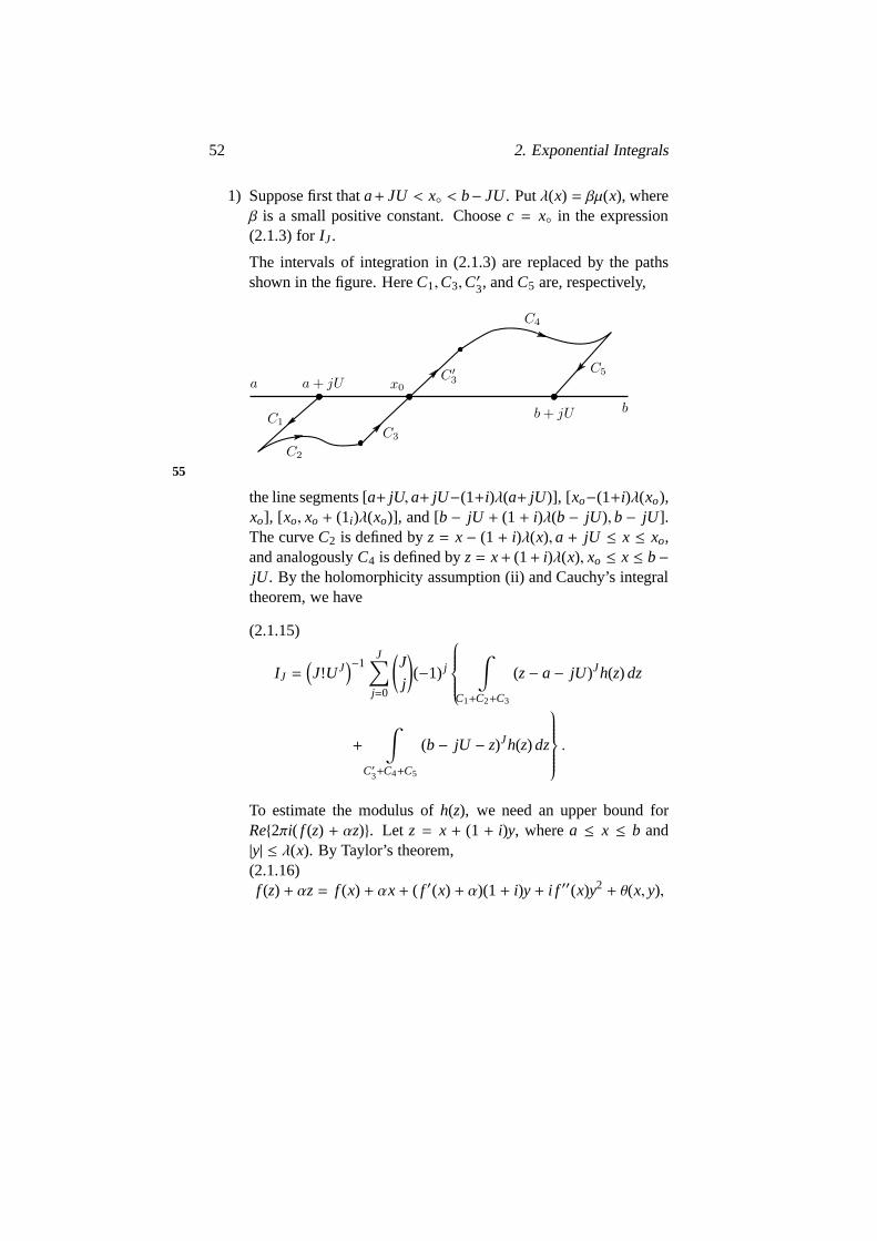
1) Suppose first thata+ JU < x◦ < b− JU. Putλ(x) = βµ(x), whereβ is a small positive constant. Choosec = x◦ in the expression(2.1.3) forIJ.
The intervals of integration in (2.1.3) are replaced by the pathsshown in the figure. HereC1,C3,C′3, andC5 are, respectively,
55
the line segments [a+ jU, a+ jU−(1+i)λ(a+ jU )], [xo−(1+i)λ(xo),xo], [xo, xo + (1i)λ(xo)], and [b− jU + (1+ i)λ(b− jU ), b− jU ].The curveC2 is defined byz = x− (1+ i)λ(x), a + jU ≤ x ≤ xo,and analogouslyC4 is defined byz= x+ (1+ i)λ(x), xo ≤ x ≤ b−jU . By the holomorphicity assumption (ii) and Cauchy’s integraltheorem, we have
IJ =(
J!UJ)−1
J∑
j=0
(
Jj
)
(−1) j
∫
C1+C2+C3
(z− a− jU )Jh(z) dz
(2.1.15)
+
∫
C′3+C4+C5
(b− jU − z)Jh(z) dz
.
To estimate the modulus ofh(z), we need an upper bound forRe{2πi( f (z) + αz)}. Let z = x + (1 + i)y, wherea ≤ x ≤ b and|y| ≤ λ(x). By Taylor’s theorem,(2.1.16)f (z) + αz= f (x) + αx+ ( f ′(x) + α)(1+ i)y+ i f ′′(x)y2 + θ(x, y),
2.1. A Saddle-Point Theorem for 53
where
θ(x, y) =∞∑
n=3
(
f (n)(x)/n!)
((1+ i)y)n.
By (2.1.6), we have
|θ(x, y)| ≪ F(x)|y|3µ(x)−3,
so that by (iv) 56
|θ(x, y)| ≤ 12
y2 f ′′(x)
if β is supposed to be sufficiently small. Then (2.1.16) gives
(2.1.17) Re{2πi( f (z) + αz)} ≤ −2π( f ′(x) + α)y− π f ′′(x)y2
for a ≤ x ≤ b and|y| ≤ λ(x).
Consider, in particular, the casey = sgn( f ′(x) + α)λ(x), whichoccurs in the estimation of the integrals overC2 andC4. The righthand side of (2.1.17) is now at most
−A| f ′(x) + α|µ(x) − AF(x).
In the cases|α| ≥ 2| f ′(x)| and|α| < 2| f ′(x)| this is
≤ −A|α|µ(x) − AF(x)
and≤ −AF(x) ≤ −A|α|µ(x) − AF(x),
respectively. Hence forz ∈ C2 ∪C4
(2.1.18) |h(z)| ≪ G(x) exp(−A|α|µ(x) − AF(x)).
The pathsCi for i = 1, 2, 4 and 5 depend onj, so that for claritywe denote them byCi( j). Let us first estimate the contributionof the integrals over theC2( j) andC4( j) to IJ. By the identity(2.1.5), the integrands in (2.1.15) combine to give simplyh(z) onC2( j)∪C3∪C′3∪C4( j), hence in particular onC2( j)∪C4( j). Thus,
54 2. Exponential Integrals
by (2.1.18) and the assumption (v), viz.µ′(x) ≪ 1, the integralsin (2.1.15) restricted toC2( j) andC4( j) contribute 57
≪b−JU∫
a+JU
G(x) exp(−A|α|µ(x) − AF(x)) dx.
Integrals over the other parts of theC2( j) andC4( j) are estimatedsimilarly, but noting that the function in front ofh(z) is now≪1+(µ(x)/U)J. In this way it is seen that the integrals over theC2( j)andC4( j) give together at most the first error term in (2.1.11).
Next we turn to the integrals over theC1( j) andC5( j). By (2.1.17)we have
∫
C1( j)
(z− a− jU )Jh(z) dz≪ G(a+ jU )
∞∫
◦
yJ exp(−2π| f ′(a+ jU )
+ α|y− π f ′′(a+ jU )y2) dy
≪ EJ(a+ jU ),
and similarly for the integrals over theC5( j). Hence these inte-grals contribute the last error term in (2.1.11).
Finally, as was noted above, the integrals overC3 + C′3 give to-gether the integral
(2.1.19) K = (1+ i)
λ(x◦)∫
−λ(x◦)
h(x◦ + (1+ i)y) dy.
Applying Taylor’s theorem and similar arguments as in the proofof (2.1.17), we find that for|y| ≤ λ(x◦)(2.1.20)
g(xo + (1+ i)y) = g(xo) + g′(xo)(1+ i)y+ o(
G(xo)µ(xo)−2y2)
,
or, more crudely,
(2.1.21) g(x◦ + (1+ i)y) = g(x◦) + o(
G(x◦)µ(x◦)−1|y|
)
,
2.1. A Saddle-Point Theorem for 55
and analogously
f (x◦ + (1+ i)y) + α(x◦ + (1+ i)y) = f (x◦) + αx◦
(2.1.22)
+ i f ′′(x◦)y2 +
16
f ′′′(x◦) (1+ i)3y3 + o(
F(x◦)µ(x◦)−4y4
)
= f (x◦) + αx◦ + i f ′′(x◦)y2 + o
(
F(x◦)µ(x◦)−3|y|3
)
.
(2.1.23)
58
Let
(2.1.24) v = λ(x◦)F(x◦)−1/3,
and writeK = K1 + K2 + K3, where the integralsK1,K2, andK3
are taken over the intervals [−λ(x◦),−v], [−v, v], and [v, λ(x◦)],respectively.
First, by (2.1.17) we have
K1 + K3 ≪ G(x◦)
∞∫
v
exp(
−π f ′′(x◦)y2)
dy
≪ G(x◦)v−1 f ′′(x◦)
−1 exp(
−πv2 f ′′(x◦))
≪ G(x◦)µ(x◦)F(x◦)−2/3 exp
(
−AF(x◦)1/3
)
,
whence by (vi)
(2.1.25) K1 + K3 ≪ G(x◦)µ(x◦)F(x◦)−3/2.
The integralK2, which will give the saddle-point term is evaluatedby applying (2.1.20) and (2.1.22). The latter implies that for |y| ≤v
e( f (x◦ + (1+ i)) + α (x◦ + (1+ i)y))(2.1.26)
= e( f (x◦) + αx◦) exp(
−2π f ′′(x◦)y2)
×
56 2. Exponential Integrals
×{
1+13πi f ′′(x◦) (1+ i)3y3 + o
(
F(x◦)µ(x◦)−4y4
)
+ o(
F(x◦)2µ(x◦)
−6y6)
}
;
note that the last two terms in (2.1.22) are≪ 1 by the choice(2.1.24) ofv. When this equation is multiplied by (2.1.20) and59
the product is integrated over the interval [−v, v], the integrals ofthose explicit terms involving odd powers ofy vanish, and we endup with
K2 = (1+ i)g(x◦)e( f (x◦) + αx◦)
v∫
−v
exp(
−2π f ′′(x◦)y2)
dy
(2.1.27)
+o
G(x◦)
v∫
−v
exp(
−2π f ′′(x◦)y2) (
µ(x◦)−2y2 + F(x◦)µ(x◦)
−4y4+
F(x◦)2µ(x◦)
−6y6)
dy)
.
In the main term, the integration can be extended to the wholelinewith an error≪ G(x◦)µ(x◦)F(x◦)−3/2, and since
(2.1.28)
∞∫
−∞
exp(
−cy2)
dy= (π/c)1/2(c > 0),
the leading term in (2.1.27) gives the leading term in (2.1.11) withξ(x◦) = 1, in accordance with (2.1.12). Further, as a generaliza-tion of (2.1.28), we have
(2.1.29)
∞∫
−∞
exp(
−cy2)
y2ν dy= dνc−ν−1/2(c > 0, ν ≥ 0)
where thedν are certain numerical constants, and by using this theerror terms in (2.1.27) are seen to be≪ G(x◦)µ(x◦)F(x◦)−3/2.
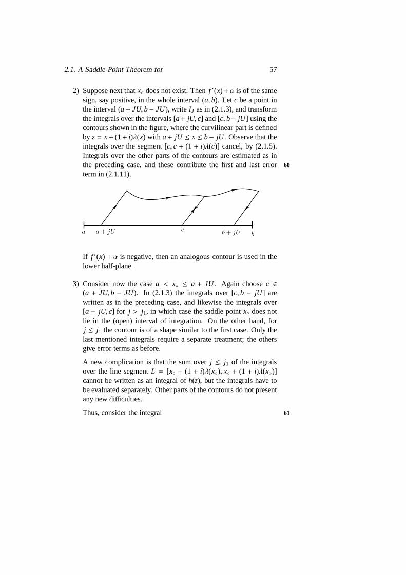
2.1. A Saddle-Point Theorem for 57
2) Suppose next thatx◦ does not exist. Thenf ′(x)+ α is of the samesign, say positive, in the whole interval (a, b). Let c be a point inthe interval (a+ JU, b− JU), write IJ as in (2.1.3), and transformthe integrals over the intervals [a+ jU, c] and [c, b− jU ] using thecontours shown in the figure, where the curvilinear part is definedby z= x+ (1+ i)λ(x) with a+ jU ≤ x ≤ b− jU . Observe that theintegrals over the segment [c, c + (1 + i)λ(c)] cancel, by (2.1.5).Integrals over the other parts of the contours are estimatedas inthe preceding case, and these contribute the first and last error 60
term in (2.1.11).
If f ′(x) + α is negative, then an analogous contour is used in thelower half-plane.
3) Consider now the casea < x◦ ≤ a + JU. Again choosec ∈(a + JU, b − JU). In (2.1.3) the integrals over [c, b − jU ] arewritten as in the preceding case, and likewise the integralsover[a + jU, c] for j > j1, in which case the saddle pointx◦ does notlie in the (open) interval of integration. On the other hand,forj ≤ j1 the contour is of a shape similar to the first case. Only thelast mentioned integrals require a separate treatment; theothersgive error terms as before.
A new complication is that the sum overj ≤ j1 of the integralsover the line segmentL = [x◦ − (1 + i)λ(x◦), x◦ + (1 + i)λ(x◦)]cannot be written as an integral ofh(z), but the integrals have tobe evaluated separately. Other parts of the contours do not presentany new difficulties.
Thus, consider the integral 61
58 2. Exponential Integrals
(2.1.30) K = U−J∫
L
(z− a− jU )Jh(z) dz.
This is of the same type as the integralK in (2.1.19) - withg(z)replaced byU−J(z− a − jU )Jg(z) - so that in principle it wouldbe possible to apply the result of the previous discussion assuch.But then the functionG(x) would have to be replaced byU−Jµ(x)J
G(x), which may become large ifJ is large. Therefore we modifythe argument in order to prevent the error term from becomingimpracticably large.
But the first step in the treatment of the integralK is as before.Namely, letv be as in (2.1.24), putz = x◦ + (1 + i)y, and letK1 and K3 be the integrals with respect toy over the intervals[−λ(x◦),−v] and [v, λ(x◦)]. ThenK1 + K3 can be estimated as be-fore, except that the extra factor 1+ (v/U)J has to be inserted. Butsince (v/U)J ≪ F(x◦)J/6 by (2.1.10) and (2.1.24), the estimate(2.1.25) remains valid even for the new integralsK1 andK3.
The new integralK2, which represents the main part ofK, is now
K2 = (1+ i)U−J
v∫
−v
(x◦ − a− jU + (1+ i)y)Jh(x◦ + (1+ i)y) dy.
For the functionh(x◦ + (1+ i)y) we are going to use a somewhatcruder approximation than before. By (2.1.21) and (2.1.23)wehave
h(x◦ + (1+ i)y)(2.1.31)
={
g(x◦)e( f (x◦) + αx◦) + o(
G(x◦)µ(x◦)−1|y|
)
+o(
F(x◦)G(x◦)µ(x◦)−3|y|3
)}
× exp(
−2π f ′′(x◦)y2)
.
Since by (2.1.29), (2.1.10), and (iv)62
U−J
v∫
−v
(
UJ + |y|J)
|y|ν exp(
−2π f ′′(x◦)y2)
dy
2.1. A Saddle-Point Theorem for 59
≪ f ′′(x◦)−(ν+1)/2 + U−J f ′′(x◦)
−(ν+J+1)/2
≪ µ(x◦)ν+1F(x◦)
−(ν+1)/2
the contribution of the error terms in (2.1.31) toK2 is≪ G(x◦)µ(x◦) F(x◦)−1. Hence
K2 =√
2g(x◦)e( f (x◦) + αx◦ + 1/8)U−J
v∫
−v
(x◦ − a− jU + (1+ i)y)J
exp(
−2π f ′′(x◦)y2)
dy+ o(
G(x◦)µ(x◦)F(x◦)−1)
=√
2g(x◦)e( f (x◦) + αx◦ + 1/8) U−J∑
0≤ν≤J/2
(x◦ − a− jU )J−2ν×
× (1+ i)2ν
(
J2ν
)
v∫
−v
y2ν exp(
−2π f ′′(x◦)y2)
dy
+ o(
G(x◦)µ(x◦)F(x◦)−1)
.
As before, the integrals here can be extended to the whole realline with a negligible error. Then, evaluating the new integrals by(2.1.29) we find that with
cν = 2−νπ−ν−1/2(1+ i)2ν(
J2ν
)
dν
and withξ(x◦) as in (2.1.13), the resulting expression forIJ is asin (2.1.11).
4) The remaining caseb− jU ≤ x◦ < b is analogous to the precedingone.
�
Remark . If f satisfies the conditions of Theorem 2.1 and 2.2 exceptthat f ′′(x) is negative in the interval [a, b], then the results hold with the63
minor modifications that in the main term the factore( f (x◦)+αx◦+1/8)is to be replaced bye( f (x◦) + αx◦ − 1/8), and| f ′′(x◦)| should stand inplace of f ′′(x◦).
60 2. Exponential Integrals
2.2 Smoothed Exponential Integrals without a Sad-dle Point
Theorem 2.2 covers also the case of exponential integralsIJ without asaddle point. However, in applications, the condition (iv)on f ′′ maynot be fulfilled. Nevertheless, if the assumption off ′ is strengthened,then no assumption onf ′′ is needed. The next theorem is a result of thiskind.
Theorem 2.3. Suppose that the functions f and g satisfy the conditions(i) and (ii) in the preceding section, withµ(x) = µ, a constant. Supposealso that
|g(z)| ≪ G for z∈ D,(2.2.1)
| f ′(x)| ≍ M for a ≤ x ≤ b,(2.2.2)
and
| f ′(z)| ≪ M for z ∈ D.(2.2.3)
Let IJ be as in(2.1.2)with α = 0 and0 < JU < (b− a)/2. Then
(2.2.4) IJ ≪ U−JGM−J−1 +(
µJU1−J + b− a)
Ge−AMµ .
Proof. By (2.2.2), the functionf ′(x) cannot change its sign in the inter-val [a, b]. Suppose, to be specific, thatf ′(x) is positive. By (2.2.3) andCauchy’s integral formula we have
| f (k)(x)| ≪ k!M(µ/2)−k+1 for k = 1, 2, . . . and a ≤ x ≤ b.
Then, by (2.2.2) and Taylor’s theorem, it is seen that
(2.2.5) Re(2πi f (z)) < −AMy
for z = x+ yi, a ≤ x ≤ b, and 0≤ y ≤ βµ = λ, whereβ is a sufficiently64
small positive constant. �
2.2. Smoothed Exponential Integrals without a Saddle Point 61
Now, for a proof of (2.2.4), the integralIJ is written as in (2.1.3),where the intervals [a+ jU, c] and [c, b− jU ] are deformed to rectangularcontours respectively with verticesa+ jU, a+ jU + iλ, c+ iλ, andc, orc, c+ iλ, b− jU + iλ, andb− jU . Then (2.2.4) follows easily by (2.2.1),(2.2.5) and (2.1.5).
Notes
In the saddle-point lemma of Atkinson (Lemma 1 in [2]), the assump-tions on the functionsF andµ are weaker than those in Theorem 2.2,for the conditions (v) and (vi) are missing. Actually we posed these justfor simplicity. On the other hand, one of the conditions in [2] is strongerthan ours, for in place of (iv) there is an upper bound forf ′′(z)−1 forz ∈ D. However, in the proof this is needed only on the real interval[a, b], in which case it coincides with (iv).
The complications that arose in Theorem 2.2 whenx◦ lies neara orb seem inevitable, for then the integrand is almost stationary neara orb, and consequently there is not so much to be gained by smoothing.
The caseJ = 1 of Theorem 2.3 is Lemma 2 in [16] and Lemma 2.3in [13]. Our proof is not a direct generalization of that in [16] whichturned out to become somewhat tedious for generalJ.
Theorems 2.2 and 2.3 may be useful in problems in which the stan- 65
dard results (corresponding toJ = 0) on exponential integrals are notaccurate enough. An example of such an application is the improvementof the error terms in the approximate functional equations for ζ2(s) andϕ(s) in [19].
The parametersU and J, which determine the smoothing, can bechosen differently ata andb. Such a version of Theorem 2.2 is given in[19], and the proof is practically the same. The corresponding smoothedintegrals is of the type
U−JV−K
U∫
◦
du1 · · ·U
∫
◦
duJ
V∫
◦
dv1 · · ·V
∫
◦
dvK
b−v∫
a+u
h(x) dx,
62 2. Exponential Integrals
whereu = u1 + · · · + uJ andv = v1 + · · · + vK . ForU = V andJ = K,this amounts to the integralIJ in (2.1.2).
Chapter 3
Transformation Formulaefor Exponential Sums
THE BASIC RESULTS of these notes, formulae relating exponential 66
sums∑
M1≤m≤M2
b(m)g(m)e( f (m) = d(m) or a(m),
or their smoothed versions, to other exponential sums involving thesameb(m), are established in this chapter by combining the summationformulae of Chapter 1 with the theorems of Chapter 2 on exponentialintegrals. The theorems in [16] and [17] concerning Dirichlet polyno-mials (which will be discussed in§ 4.1) were the first examples of suchresults. As will be seen, the methods of these papers work even in thepresent more general context without any extra effort.
3.1 Transformation of Exponential Sums
To begin with, we derive a transformation formula for the above men-tioned sum withb(m) = d(m). The proof is modelled on that of Theorem1 in [16].
In the following theorems,δ1, δ2, . . . denote positive constants whichmay be supposed to be arbitrarily small. Further, putL = log M1 forshort.
63
64 3. Transformation Formulae for Exponential Sums
Theorem 3.1.Let2 ≤ M1 < M2 ≤ 2M1, and let f and g be holomorphicfunctions in the domain
(3.1.1) D = {z |z− x| < cM1 for some x∈ [M1,M2]} ,
where c is a positive constant. Suppose that f(x) is real for M1 ≤ x ≤67
M2. Suppose also that, for some positive numbers F and G,
|g(z)| ≪ G,(3.1.2)
| f ′(z)| ≪ FM−11(3.1.3)
for z ∈ D, and that
(3.1.4) (0<) f ′′(x) ≫ FM−21 for M1 ≤ x ≤ M2.
Let r = h/k be a rational number such that
1 ≤ k≪ M1/2−δ11 ,(3.1.5)
|r | ≍ FM−11(3.1.6)
and
f ′(M(r)) = r(3.1.7)
for a certain number M(r) ∈ (M1,M2). Write
M j = M(r) + (−1) jmj , j = 1, 2.
Suppose that m1 ≍ m2, and that
(3.1.8) Mδ21 max
(
M1F−1/2, |hk|)
≪ m1 ≪ M1−δ31 .
Define for j= 1, 2
p j,n(x) = f (x) − rx + (−1) j−1(
2√
nx/k− 1/8)
,(3.1.9)
n j =(
r − f ′(
M j
))2k2M j ,(3.1.10)

3.1. Transformation of Exponential Sums 65
and for n < n j let xj,n be the (unique) zero of p′j,n(x) in the interval(M1,M2). Then
∑
M1≤m≤M2
d(m)g(m)e( f (m))(3.1.11)
= k−1 (
log M(r) + 2γ − 2 logk)
g(M(r)) f ′′(M(r))−1/2e( f (M(r))
−rM (r) + 1/8)+ +i2−1/2k−1/22
∑
j=1
(−1) j−1
∑
n<nj
d(n)ek
(
−nh)
n−1/4x−1/4j,n g
(
x j,n
)
p′′j,n(
x j,n
)−1/2×
×e(
p j,n(x j,n) + 1/8)
+ o(
FGh−2km−11 L
)
+ o(
G(|h|)1/2m1/21 L2
)
+
+o(
F1/2G|h|−3/4k5/4m−1/41 L
)
.
68
Proof. Suppose, to be specific, thatr > 0, and thush > 0. The proof issimilar for r < 0.
The assertion (3.1.11) should be understood as an asymptotic result,in which M1 and M2 are large. Then the numbersF and n j are alsolarge. In fact,
F ≫ M1/2+δ11(3.1.12)
and
n j ≫ hkM2δ21 .(3.1.13)
For a proof of (3.1.12), note that by (3.1.6) and (3.1.5)
F ≫ M1r ≥ k−1M1 ≫ M1/2+δ11 .
Consider next the order ofn j . By (3.1.1) and the holomorphicity off in the domain (3.1.1) we havef ′′(x) ≪ FM−2
1 , which implies togetherwith (3.1.4) that
(3.1.14) f ′′(x) ≍ FM−21 for M1 ≤ x ≤ M2.

66 3. Transformation Formulae for Exponential Sums
Thus, by (3.1.7),∣
∣
∣
∣
r − f ′(
M j
)
∣
∣
∣
∣
≍ mjFM−21 ,(3.1.15)
so that by (3.1.10) and (3.1.6) we have
n j ≍ F2k2m2j M−31 ≍ F−1h3k−1m2
j .(3.1.16)
69
This gives (3.1.13) owing to the estimatesmj ≫ M1+δ21 F−1/2 and
F ≪ M1r. Also, it follows thatn j ≪ MA1 , for h≪ M1 andmj ≪ M1 by
(3.1.8).The numbersn j are determined by the condition
(3.1.17) p′j,nj
(
M j
)
= 0.
Then clearly(−1) j p′j,n
(
M j
)
> 0 for n < n j .
On the other hand, by (3.1.7)
(−1) j p′j,n(M(r)) = −n1/2M(r)−1/2k−1 < 0
for all positive n. Consequently, forn < n j there is a zerox j,n ofp′j,n(x) in the interval (M1,M2), and moreoverx1,n ∈ (M1,M(r)), x2,n ∈(M(r),M2). Also, it is clear thatp′j,n has no zero in the interval (M1,M2)if n ≥ n j .
To prove the uniqueness ofx j,n, we show thatp′′j,n is positive andthusp′j,n is increasing in the interval [M1,M2]. In fact,
(3.1.18) p′′j,n(x) ≍ FM−21 for M1 ≤ x ≤ M2, n ≤ 2n j ,
at least ifM1 is supposed to be sufficiently large. For by definition
p′′j,n(x) = f ′′(x) + (−1) j 12
n1/2x−3/2k−1,
where by (3.1.16) and (3.1.8)
n1/2x−3/2k−1 ≪ Fm1M−31 ≪ FM−2−δ3
1 ,

3.1. Transformation of Exponential Sums 67
so that by (3.1.14) the termf ′′(x) dominates.70
After these preliminaries we may go into the proof of the formula(3.1.11). Denote by 5 the sum under consideration. Actuallyit is easierto deal with the smoothed sum
S′ = U−1
U∫
◦
S(u) du,(3.1.19)
where
S(u) =∑
M1+u≤m≤M2−u
d(m)g(m)e( f (m)).(3.1.20)
The parameterU will be chosen later in an optimal way; presentlywe suppose only that
(3.1.21) Mδ41 ≪ U ≤ 1
2min(m1,m2) .
Since∑
x≤n≤x+y
d(n) ≪ y log x for xǫ ≪ y≪ x,(3.1.22)
(see [25]), we have
S − S′ ≪ GUL.(3.1.23)
The summation formula (1.9.1) is now applied to the sumS(u),which is first written as
S(u) =∑
a≤m≤b
d(m)g(m)e( f (m) −mr)e(mr),
with a = M1+u, b = M2−u. We may assume that neither of the numbersa andb is an integer, for the value ofS(u) for the finitely many othervalues ofu is irrelevant in the integral (3.1.19). Then by (1.9.1)
S(u) = k−1
b∫
a
(log x+ 2γ − 2 logk)g(x)e( f (x) − rx) dx
(3.1.24)
68 3. Transformation Formulae for Exponential Sums
+ k−1∞∑
n=1
d(n)
b∫
a
{
−2πek
(
−nh)
Y◦(
4π√
nx/k)
+ 4ek
(
nh)
K◦(
4π√
nx/k)}
g(x)e( f (x) − rx) dx
= k−1
I◦ +∞∑
n=1
d(n)(
ek
(
−nh)
In + ek
(
nh)
in)
,
say.71
The integralsin are very small and quite negligible. Indeed, by(3.1.5) we have
√nM1/k≫
√nMδ1
1 , so that by (1.3.17)
k−1∞∑
n=1
d(n) |in| ≪ k−1GM1
∞∑
n=1
d(n) exp(
−A√
nMδ11
)
(3.1.25)
≪ Gexp(
−AMδ11
)
.
Consider next the integralI◦. We apply Theorem 2.1 withα = −randµ(x) a constant function≍ M1. The assumptions of Theorem 2.1are satisfied in virtue of the conditions of our theorem. By (3.1.7), thesaddle point isM(r). Hence the saddle-point term fork−1I◦ equals theleading term in (3.1.11).
The first error term in (2.1.9) is
≪ LGM1 exp(−AF)
which is negligible by (3.1.12).The last two error terms contribute
(3.1.26)
≪ GL{
(∣
∣
∣ f ′(a) − r∣
∣
∣ + F1/2M−11
)−1+
(∣
∣
∣ f ′(b) − r∣
∣
∣ + F1/2M−11
)−1}
.
For same reasons as in (3.1.15), we have∣
∣
∣ f ′(a) − r∣
∣
∣ ≍ Fm1M−21 ,
and likewise for| f ′(b) − r |. Hence the expression (3.1.26) is≪ F−1
Gm−11 M2
1L, which is further≪ FGm−11 r−2L by (3.1.6). The second error72

3.1. Transformation of Exponential Sums 69
term in (2.1.9), viz.o(GM1F−3/2L), can be absorbed into this, for
M1F−3/2 ≪ r−1 ≪ FM−11 r−2 ≪ Fm−1
1 r−2.
Hence the error terms fork−1I◦ give togethero(FGh−2km−11 L),
which is the first error term in (3.1.11).We are now left with the integrals
(3.1.27) In = −2π
b∫
a
Y◦(
4π√
nx/k)
g(x)e( f (x) − rx) dx.
By (1.3.9), the functionY◦ can be written in terms of Hankel func-tions as
Y◦(z) =12i
(
H(1)◦ (z) − H(2)
◦ (z))
,(3.1.28)
where by (1.3.13)
H( j)◦ (z) =
(
2πz
)1/2
exp
(
(−1) j−1i
(
z−14π
))
(
1+ g j(z))
.(3.1.29)
The functionsg j(z) are holomorphic in the half-planeRe z> 0, andby (1.3.14)
(3.1.30)∣
∣
∣g j(z)∣
∣
∣ ≪ |z|−1 for |z| ≥ 1,Re z> 0.
By (3.1.27) - (3.1.29) we may write
In = I (1)n − I (2)
n ,(3.1.31)
where
I ( j)n = i2−1/2k1/2n−1/4
b∫
a
x−1/4g(x)(
1+ g j
(
4π√
nx/k))
e(
p j,n(x))
dx.
(3.1.32)
70 3. Transformation Formulae for Exponential Sums
For n ≤ 2n j we apply Theorem 2.1 toI ( j)n , again withα = −r. The 73
functionf (x) + (−1) j−1
(
2√
nx/k− 1/8)
now stands for the functionf , and moreoverµ(x) ≍ M1 andF(x) = F.The conditions of the theorem are satisfied, in particular the validity ofthe condition (iv) onf ′′ follows from (3.1.18), and the condition (iii)on f ′ can be checked by (3.1.3) and (3.1.16). The numberx j,n is, bydefinition, the saddle point forI ( j)
n , and it lies in the interval (M1,M2)if and only if n < n j . However, inI ( j)
n the interval of integration is[a, b] = [M1+u,M2−u], andx j,n ∈ (a, b) if and only if n < n j(u), where
(3.1.33) n j(u) =(
r − f ′(
M j + (−1) j−1u))2
k2(
M j + (−1) j−1u)
in analogy with (3.1.10). But for simplicity we count the saddle-pointterms for alln < n j , and the number of superfluous terms is then
(3.1.34) ≪ 1+ n j − n j(U)≪ 1+ F2k2m1M−31 U.
The saddle-point term fork−1I ( j)n is
i2−1/2k−1/2n−1/4x−1/4j,n g
(
x j,n
) (
1+ g j
(
4π√
nxj,n/k))
×(3.1.35)
×p′′j,n(
x j,n
)−1/2e(
p j,n
(
x j,n
)
+ 1/8)
.
Multiplied by (−1) j−1d(n)ek(−nh), these agree, up tog j(. . .), withthe individual terms of the sums on the right of (3.1.11). Theeffect ofthe omission ofg j(. . .) is by (3.1.30), (3.1.16), (3.1.18), and (3.1.5)
≪ F−1/2Gk1/2M1/41
∑
n≪M1
d(n)n−3/4
≪ Gkm1/21 M−1/2
1 L ≪ Gm1/21 L,
which can be absorbed into the second error term in (3.1.11).74
The extra saddle-point terms, counted in (3.1.34), contribute at most
≪(
1+ F2k2m1M−31 U
)
F−1/2Gk−1/2M3/4+ǫ1 n−1/4
1 ,
3.1. Transformation of Exponential Sums 71
which, by (3.1.16) and (3.1.6), is
(3.1.36) ≪ F1/2Gh−3/2k1/2m−1/21 Mǫ
1 + F−1/2Gh3/2k−1/2m1/21 Mǫ
1U.
Now, allowing for these error terms, we have the same saddle-pointterms given in (3.1.11), for all sumsS(u), and hence by (3.1.19) forS′,too.
Consider now the error terms when Theorem 2.1 is applied toI ( j)n
for n ≤ 2n j . The first error term in (2.1.9) is clearly negligible. Further,the contribution of the error terms involvingx◦ to S(u) is
≪ F−3/2Gk−1/2M3/41
∑
n≪n1
d(n)n−1/4,
which, by (3.1.16), (3.1.8) and (3.1.5), is
≪ Gkm3/21 M−3/2
1 L ≪ Gkm1/21 M−1/2
1 L ≪ Gm1/21 .
This is smaller than the second error term in (3.1.11).The last two error terms are similar, so it suffices to considero(E◦(a))
as an example. By (2.1.8) and (3.1.32), this error term fork−1I ( j)n is
≪ Gk−1/2M−1/41 n−1/4
(∣
∣
∣p′j,n(a)∣
∣
∣ + p′′j,n(a)1/2)−1
.
Consider the casej = 1; the casej = 2 is less critical since|p′2,n(a)|cannot be small. Nowp′1,n1(u)(a) = 0 andp′′1,n(a) ≍ F−1r2, so it is easily 75
seen that
(∣
∣
∣p′1,n(a)∣
∣
∣ + p′′1,n(a)1/2)−1≪
F1/2r−1 for |n− n1(u)| ≪ F−1/2h2m1,
kM1/21 n1/2
1 |n− n1(u)|−1 otherwise
Note that by (3.1.8) and (3.1.6)
F−1/2h2m1 ≫ F−1h2M1+δ21 ≫ hkMδ2
1 .
Hence, by (3.1.22), the mean value ofd(n) in the interval|n− n1(u)|≪ F−1/2h2m1 can be estimated aso(L). It is now easily seen that thecontribution toS(u) of the error terms in question is
≪ Gh1/2k1/2m1/21 L2,
72 3. Transformation Formulae for Exponential Sums
which is the second error term in (3.1.11).The smoothing device was introduced with the integralsI ( j)
n for n >2n j in mind. By (3.1.19), (3.1.24), (3.1.31), and (3.1.32), their contribu-tion to S′ is equal to
i2−1/2k−1/22
∑
j=1
(−1) j−1∑
n>2nj
d(n)ek
(
−nh)
n−1/4×(3.1.37)
×M2∫
M1
η1(x)x−1/4g(x)(
1+ g j
(
4π√
nx/k))
e(
p j,n(x))
dx,
whereη1(x) is a weight function in the sense of Chapter 2, withJ = 1andU being the other smoothing parameter. The series in (3.1.24)isboundedly convergent with respect tou, by Theorem 1.7, so that it canbe integrated term by term.
The smoothed exponential integrals in (3.1.37) are estimated byTheorem 2.3, wherep j,n(z) stands forf (z), andµ ≍ m1. To begin with,76
we have to check that the conditions of this theorem are satisfied. Wehave
p′j,n(z) = f ′(z) − r + (−1) j−1n1/2z−1/2k−1.
Let n > 2n j , and letz lie in the domainD, sayD◦, of Theorem 2.3.Then by (3.1.16)
∣
∣
∣n1/2z−1/2k−1∣
∣
∣ ≫ m1FM−21 .
On the other hand, sincef ′(M(r)) − r = 0 and| f ′′(z)| ≪ FM−21 for
z ∈ D◦ by (3.1.3) and Cauchy’s integral formula, we also have
| f ′(z) − r | ≪ m1FM−21 .
Thus, the condition (2.2.3) holds with
(3.1.38) M = k−1M−1/21 n1/2.
Further, to verify the condition (2.2.2), comparep′j,n(x) with p′j,nj(x),
using (3.1.17) and the fact thatp′j,nj(x) is increasing in the interval
[M1,M2].
3.1. Transformation of Exponential Sums 73
We may now apply the estimate (2.2.4) in (3.1.37). The secondtermon the right of (2.2.4) is exponentially small, for by (3.1.38), (3.1.16),and (3.1.8)
Mµ≫ k−1M−1/21 n1/2m1 ≫ (n/n1)1/2 Fm2
1M−21
≫ (n/n1)1/2 M2δ21 .
Hence these terms are negligible.The contribution of the termsU−1GM−2 in (2.2.4) to (3.1.37) is
≪ Gk3/2M3/41 U−1
∑
n≫n1
d(n)n−5/4
≪ Gk3/2M3/41 n−1/4
1 U−1L
≪ GF−1/2kM3/21 m−1/2
1 U−1L
≪ GFh−3/2k5/2m−1/21 U−1L.
77
Combining this with (3.1.23) and (3.1.36), we find that (3.1.11)holds, up to the additional error terms
≪ GUL+ F1/2Gh−3/2k1/2m−1/21 Mǫ
1(3.1.39)
+ F−1/2Gh3/2k−1/2m1/21 Mǫ
1U +GFh−3/2k5/2m−1/21 U−1L.
Here the second term is superseded by the last term in (3.1.11). Fur-ther, the first and last term coincide with the last term in (3.1.11) if wechoose
(3.1.40) U = F1/2h−3/4k5/4m−1/41 .
Then, by (3.1.8), the third term in (3.1.39) is
≪ Gh3/4k3/4m1/41 M1 ≪ G(hk)1/2m1/2
1 Mǫ−δ2/41 ,
which can be absorbed into the second error term in (3.1.11).It should still be verified that the numberU in (3.1.40) satisfies the
condition (3.1.21). By (3.1.8) and (3.1.6) we have
Um−11 ≪ U
(
M1+δ21 F−1/2
)−1≪ (hk)1/4m−1/4
1 M−δ21 ≪ M−δ2
1
74 3. Transformation Formulae for Exponential Sums
and also, in the other direction,
U ≫ F1/2h−3/4k5/4M−1/4+δ3/41
≫ M1/4+δ3/41 h−1/4k3/4 ≫ Mδ3/4
1
Hence (3.1.21) holds, and the proof of the theorem is complete.78
The next theorem is an analogue of Theorem 3.1 for exponentialsums involving the Fourier coefficientsa(n) of a cusp form of weightκ.The proof is omitted, because the argument is practically the same; thesummation formula (1.9.2) is just applied in place of (1.9.1). Note thatin (1.9.2) there is nothing is correspond to the first term in (1.9.1), andconsequently in the transformation formula there are no counterparts forthe first explicit term and the first error term in (3.1.11). �
Theorem 3.2. Suppose that the assumptions of Theorem 3.1 are satis-fied. Then
∑
M1≤m≤M2
a(m)g(m)e( f (m))(3.1.41)
= i2−1/2k−1/22
∑
j=1
(−1) j−1∑
n<nj
a(n)ek
(
−nh)
nκ/2+1/4×
× xκ/2−3/4j,n g
(
x j,n
)
p′′j,n(
x j,n
)−1/2e(
p j,n
(
x j,n
)
+ 1/8)
+ o(
G (|h|k)1/2 M(κ−1)/21 m1/2
1 L2)
+ o(
F1/2G|h|−3/4k5/4M(κ−1)/21 m−1/4
1 L)
.
3.2 Transformation of Smoothed Exponential Sums
We now give analogues of Theorem 3.1 and 3.2 for smoothed exponen-tial sums provided with weights of the typeηJ(n). We have to pay forthe better error terms in these new formulae by allowing certain weightsto appear in the transformed sums as well.
Theorem 3.3. Suppose that the assumptions of Theorem 3.1 are satis-fied. Let
(3.2.1) U ≫ F−1/2M1+δ41 ≍ F1/2r−1Mδ4
1 ,
3.2. Transformation of Smoothed Exponential Sums 75
and let J be a fixed positive integer exceeding a certain bound(which 79
depends onδ4). Write for j= 1, 2
M′j = M j + (−1) j−1JU = M(r) + (−1) jm′j ,
and suppose that m′j ≍ mj . Let nj be as in(3.1.10), and define analo-gously
(3.2.2) n′j =(
r − f ′(
M′j))2
k2M′j .
Then, defining the weight functionηJ(x) in the interval[M1,M2] asin (2.1.2), we have
∑
M1≤m≤M2
ηJ(m)d(m)g(m)e( f (m))(3.2.3)
= k−1 (
log M(r) + 2γ − 2 logk)
g(M(r)) f ′′(M(r))−1/2
e( f (M(r)) − rM (r) + 1/8)
+ i2−1/2k−1/22
∑
j=1
(−1) j−1∑
n<nj
w j(n)d(n)ek
(
−nh)
n−1/4x−1/4j,n ×
×(
x j,n
)
p′′j,n(
x j,n
)−1/2e(
p j,n
(
x j,n
)
+ 1/8)
+ o(
F−1G|h|3/2k−1/2m1/21 UL
)
,
where
w j(n) = 1 for n < n′j ,(3.2.4)
w j(n) ≪ 1 for n < n j ,(3.2.5)
w j(y) and w′j(y) are piecewise continuous functions in the interval(n′j ,n j) with at most J− 1 discontinuities, and
(3.2.6) w′j(y) ≪(
n j − n′j)−1
for n′j < y < n j
whenever w′j(y) exists.
76 3. Transformation Formulae for Exponential Sums
Proof. We follow the argument of the proof of Theorem 3.1, using80
however Theorem 2.2 in place of Theorem 2.1. Denoting bySJ thesmoothed sum under consideration, we have by (1.9.1), as in (3.1.24),
SJ = k−1
M2∫
M1
(
log x+ 2γ − 2 logk)
ηJ(x)g(x)e( f (x) − rx) dx
(3.2.7)
+ k−1∞∑
n=1
d(n)
M2∫
M1
{
−2πek
(
−nh)
Y◦(
4π√
nx/k)
+ 4ek
(
nh)
K◦
(
4π√
nx/k)}
ηJ(x)g(x)e( f (x) − rx) dx
= k−1
I◦ +∞∑
n=1
d(n)(ek(−nh)In + ek(nh)in)
.
As in the proof of Theorem 3.1, the integralsin are negligible.Consider next the integralI◦. We apply Theorem 2.2 choosing
µ(x) ≍ M1 again. The saddle-point isM(r), as before, and the saddle-point term forI◦ is the same as in the proof of Theorem 3.1. The firsterror term in (2.1.11) is exponentially small. The error terms involvingEJ are also negligible ifJ is taken sufficiently large (depending onδ4),since
U−1 f ′′(x)−1/2 ≪ M−δ4 for M1 ≤ x ≤ M2.
The contribution of the error termo(G(x◦)µ(x◦)F(x◦)−3/2) to k−1I◦is by (3.2.1) and (3.1.8)
≪ k−1F−3/2GM1L ≪ F−1GUL≪ F−1Gh−1/2m1/21 U,
which does not exceed the error term in (3.2.3).Turning to the integralsIn, we write as in (3.1.31) and (3.1.32)
In = I (1)n − I (2)
n ,
where81
3.2. Transformation of Smoothed Exponential Sums 77
(3.2.8)
I ( j)n = i2−1/2k1/2n−1/4
M2∫
M1
ηJ(x)−1/4g(x)(
1+ g j
(
4π√
nx/k))
e(
p j,n(x))
dx.
Let first n > 2n j . As in the proof of Theorem 3.1, we may applyTheorem 2.3 withµ ≍ m1 andM as in (3.1.38). Observe that by (3.2.1),(3.1.16), and (3.1.8)
U−1M−1 ≪ (n1/n)1/2 F−1/2m−11 M1−δ4
1 ≪ (n1/n)1/2 M−δ2−δ41
whence we we may make the termU−JGM−J−1 in (2.2.4) negligiblysmall by takingJ large enough. As before, the second term in (2.2.4) isalso negligible.
The terms forn ≤ 2n j are dealt with by Theorem 2.2. The saddlepoint terms occur again forn < n j , and they are of the same shape as in(3.1.35) except that there is the additional factor
(3.2.9) w j(n) = ξ(
x j,n
)
.
The property (3.2.4) ofw j(n) is immediate by (2.1.12), forM1 +
JU < x j,n < M2 − JU if and only if n < n′j . Further, (3.2.5) followsfrom (2.1.12) - (2.1.14) by (3.2.1) and (3.1.18). To prove the property(3.2.6), consider
w j(y) = ξ(
x j,y
)
as a function of the continuous variable in the interval (n′j , n j). Herex j,y
is the unique zero ofp′j,y(x) in the interval (M1,M1+ JU) for j = 1, andin the interval (M2 − JU,M2) for j = 2. Thusz= x j,y satisfies
f ′(z) − r + (−1) j−1y1/2z−1/2k−1 = 0.
Hence, by implicit differentiation, 82
p′′j,y(z)dxj,y
dy+
12
(−1) j−1y−1/2z−1/2k−1 = 0,
which implies that
(3.2.10)
∣
∣
∣
∣
∣
∣
dxj,y
dy
∣
∣
∣
∣
∣
∣
≍ F−1k−1M3/21 n−1/2
1 ≍ m1n−11 for n′j < y < n j .
78 3. Transformation Formulae for Exponential Sums
The functionξJ(x) in (2.1.13) and (2.1.14) is continuously differen-tiable except at the pointsa+ JU andb− jU, j = 1, . . . , J, where termsappear or disappear. By differentiation, noting thatf ′′′(x) ≪ FM−3
1 , itis easy to verify that
(3.2.11) ξ′J(x) ≪ U−1
elsewhere in the intervals (a, a+JU) and (b−JU, b). By (3.1.10), (3.2.2),and (3.1.14) we have
(3.2.12)(
n j − n′j)
n−1j ≍ m−1
1 U.
Now (3.2.6) follows from (3.2.10) - (3.2.12) at those pointsy forwhich x j,y is not of the forma+ jU or b− jU with 1 ≤ j ≤ J − 1.
As in the proof of Theorem 3.1, we may omitg j(. . .) in the saddle-point terms with an admissible error
Gkm1/21 M−1/2
1 L ≪ F−1Gh3/2k−1/2m1/21 U,
and after that these terms coincide with those in (3.2.3).Consider finally the error terms in (2.1.11) forI ( j)
n . The first of theseis clearly negligible. Also, for the same reason as in the case of I◦, theerror terms involvingEJ can be omitted ifJ is chosen sufficiently large.
Finally, the second error term in (2.1.11) fork−1I ( j)n is83
≪ F−3/2Gk−1/2M3/41 n−1/4
1 for n < n′j
and≪ F−1Gk−1/2M3/4
1 n−1/41 for n′j ≤ n < n j .
The contribution of these toSJ is
(3.2.13) ≪ F−3/2Gk−1/2M3/41 n3/4
1 L+F−1Gk−1/2M3/41 n−1/4
1
(
n j − n′j)
L.
Here we estimated the mean value ofd(n) in the interval [n′j , n j) byo(L), which is possible, by (3.1.22), for by (3.2.12), (3.1.16), (3.1.8),(3.2.1), and (3.1.6) we have
n j − n′j ≪ m−11 n1U ≪ F2k2m1M−3
1 U
3.2. Transformation of Smoothed Exponential Sums 79
≪ F2k2(
M1+δ21 F−1/2
)
M−31
(
F−1/2M1+δ41
)
≍ hkMδ2+δ41 .
By (3.2.12), the second term in (3.2.13) is
≍ F−1Gk−1/2m−11 M3/4
1 n3/41 UL,
which is of the same order as the error term in (3.2.3) and dominates thefirst term, since
m−11 U ≫
(
F−1/2M1
)
M−11 = F−1/2.
The proof of the theorem is now complete.The analogue of the preceding theorem for exponential sums involv-
ing Fourier coefficientsa(n) is as follows. The proof is similar and canbe omitted. �
Theorem 3.4. With the assumptions of Theorem 3.3, we have 84∑
M1≤m≤M2
ηJ(m)a(m)g(m)e( f (m))(3.2.14)
= i2−1/2k−1/22
∑
j=1
(−1) j−1∑
n<nj
w j(n)a(n)ek
(
−nh)
n−κ/2+1/4
× xκ/2−3/4j,n g (x− j, n) p′′j,n
(
x j,n
)−1/2e(
p j,n
(
x j,n
)
+ 1/8)
+ o(
F−1G|h|3/2k−1/2M(κ−1)/21 m1/2
1 UL)
.
Remark. In practice it is of advantage to chooseU as small as the con-dition (3.2.1) permits, i.e.
(3.2.15) U ≍ F1/2+ǫ r−1.
Then the error term in (3.2.3) is
(3.2.16) o(
F−1/2+ǫG (|h|k)1/2 m1/21
)
and that in (3.2.14) is
(3.2.17) o(
F−1/2+ǫG (|h|k)1/2 M(κ−1)/21 m1/2
1
)
.
Chapter 4
Applications
THE THEOREMS OF the preceding chapter show that the short expo-85
nential sums in quesion depend on the rational approximation of f ′(n) inthe interval of summation. But in long sums the value off ′(n) may varytoo much to be approximated accurately by a single rational number,and therefore it is necessary to split up the sum into shortersegmentssuch that in each segmentf ′(n) lies near to a certain fractionr. By suit-able averaging arguments, it is possible to add these short sums - in atransformed shape - in a non-trivial way. Variations on thistheme aregiven in§§ 4.2 - 4.4. But as a preliminary for§§ 4.2 and 4.4, we firstwork out in§ 4.1 the transformation formulae of Chapter 3 in the specialcase of Dirichlet polynomials related toζ2(s) andϕ(s).
4.1 Transformation Formulae for Dirichlet Polyno-mials
The general theorems of the preceding chapter are now applied toDirichlet polynomials
S (M1,M2) =∑
M1≤m≤M2
d(m)m−1/2−it ,(4.1.1)
Sϕ (M1,M2) =∑
M1≤m≤m2
a(m)m−k/2−it ,(4.1.2)
80
4.1. Transformation Formulae for Dirichlet Polynomials 81
as well as to their smoothed variants
S (M1,M2) =∑
M1≤m≤M2
ηJ(m)d(m)m−1/2−it ,(4.1.3)
Sϕ (M1,M2) =∑
M1≤m≤M2
ηJ(m)a(m)m−k/2−it ,(4.1.4)
whereηJ(x) is a weight function defined in (2.1.2). 86
We shall suppose for simplicity thatt is a sufficiently large positivenumber, and putL = log t. The functionχ(s) is as in the functionalequationζ(s) = χ(s)ζ(1− s), thus
χ(s) = ssπs−1 sin
(
12
sπ
)
Γ(1− s).
If σ is bounded andt tends to infinity, then (see [27], p. 68)
(4.1.5) χ(s) = (2π/t)s−1/2 ei(t+π/4)(
1+ o(
t−1))
.
Define also
(4.1.6) φ(x) = ar sinh(
x1/2)
+(
x+ x2)1/2
.
As before,δ1, δ2, . . . will denote positive constants which may besupposed to be arbitrarily small.
Theorem 4.1. Let r = h/k be a rational number such that
M1 <t
2πr< M2(4.1.7)
and
1 ≤ k≪ M1/2−δ11 .(4.1.8)
Write
M j =t
2πr+ (−1) jmj ,(4.1.9)
82 4. Applications
and suppose also that m1 ≍ m2 and
tδ2 max(
t1/2r−1, hk)
≪ m1 ≪ M1−δ31 .(4.1.10)
Let
(4.1.11) n j = h2m2j M−1j .
Then87
S(M1,M2) ={
(hk)−1/2 (
log(t/2π) + 2γ − log(hk))
(4.1.12)
+ π1/4(2hkt)−1/42
∑
j=1
∑
n<nj
d(n)e
(
n
(
hk− 1
2hk
))
n−1/4×
×(
1+πn
2hkt
)−1/4exp
(
i(−1) j−1(
2tφ(
πn2hkt
)
+π
4
))
}
r it
χ
(
12+ it
)
+ o(
h−3/2k1/2m−11 t1/2L
)
+ o(
hm1/21 t−1/2L2
)
+ o(
h−1/4k3/4m−1/41 L
)
.
Proof. We apply Theorem 3.1 with−r in place ofr, and with
f (z) = −(t/2π) logz,(4.1.13)
and
g(z) = z−1/2.(4.1.14)
Then the assumptions of the theorem are obviously satisfied with
F = t,(4.1.15)
G = M−1/21 ≍ r1/2t−1/2,(4.1.16)
and
(4.1.17) M(−r) =t
2πr.
4.1. Transformation Formulae for Dirichlet Polynomials 83
Then the numbern j in (3.1.10) equals the one in (4.1.11).The leading term on the right of (3.1.11) is
(hk)−1/2(log(t/2π) + 2γ − log(hk))r it (2π/t)itei(t+π/4)
which can also be written, by (4.1.5), as
(4.1.18) (hk)−1/2(log(t/2π) + 2γ − log(hk))r itχ
(
12+ it
)
(
1+ o(
t−1))
.
The functionp j,n(x) reads in the present case 88
(4.1.19) − (t/2π) log x+ rx + (−1) j−1(
2√
nx/k− 1/8)
and the numbersx j,n are roots of the equation
(4.1.20) p′j,n = −t
2πx+ r + (−1) j−1n1/2x−1/2k−1 = 0,
and thus roots of the quadratic equation
(4.1.21) x2 −( tπr+
n
h2
)
x+( t2πr
)2= 0.
Moreover, sincex1,n < x2,n, we have
x j,n =t
2πr+
n
2h2+
(−1) j
h2
(
n2
4+
hknt2π
)1/2
(4.1.22)
and
(t/2πr)2x−1j,n =
t2πr+
n
2h2−
(−1) j
h2
(
n2
4+
hknt2π
)1/2
.(4.1.23)
Next we show that(4.1.24)
2−1/2k−1/2x−3/4j,n p′′j,n
(
x j,n
)−1/2= π1/4(2hkt)−1/4
(
1+πn
2hkt
)−1/4.
Indeed, by (4.1.19) we have
2kx3/2j,n p′′j,n
(
x j,n
)
= π−1ktx−1/2j,n + (−1) jn1/2,
84 4. Applications
which by (4.1.20) and (4.1.23) is further equal to
(−1) j−1h2n−1/2(
2( t2πr
)2x−1
j,n −tπr
)
+ (−1) jn1/2
= π−1/2(2hkt)1/2(
1+πn
2hkt
)1/2.
This proves (4.1.24).To complete the calculation of the explicit terms in (3.1.11), we still89
have to work outp j,n(x j,n). Note that by (4.1.22) and (4.1.23)
(
2πrt−1x j,n
)
(−1) j = 1+πnhkt+
(
(
πnhkt
)2+
2πnhkt
)1/2
=
(
(
πn2hkt
)1/2+
(
1+πn
2hkt
)1/2)2
,
whence
(4.1.25) log(
2πrt−1x j,n
)
= (−1) j2ar sinh
(
(
πn2hkt
)1/2)
.
Also, by (4.1.20) and (4.1.22),
2πrx j,n + 4π(−1) j−1n1/2x1/2j,n k−1
= 2t − 2πrx j,n
= t −πnhk+ (−1) j−12t
(
πn2hkt
+
(
πn2hkt
)2)1/2
Together with (4.1.19), (4.1.25), and (4.1.6), this gives
2πp j,n
(
x j,n
)
= (−1) j−1(
2tφ(
πn2hkt
)
−π
4
)
− t log(t(2π) + t log r + t −πnhk.
Hence, using (4.1.5) again, we have
i(−1) j−1e(
p j,n
(
x j,n
)
+ 1/8)
=(4.1.26)
= e(
−n
2hk
)
exp(
i(−1) j−1(
2tφ(
πn2hkt
)
+π
4
))
r it
4.1. Transformation Formulae for Dirichlet Polynomials 85
χ
(
12+ it
)
(
1+ 0(
t−1))
.
By (4.1.18), (4.1.24), and (4.1.26), we find that the explicit termson the right of (3.1.11) coincide with those in (4.1.12), up to the factor1+ o(t−1). The correctiono(t−1) can be omitted with an error
≪ t−1(
(hk)−1/2L + (hkt)−1/4n3/41 L
)
,
which is 90
≪ t−1(
(hk)−1/2L + t−1h2k−1m3/21 L
)
≪ hm1/21 t−1L(4.1.27)
by (4.1.11), (4.1.7), and (4.1.10). This is clearly negligible in (4.1.12).Finally, the error terms in (3.1.11) give those in (4.1.12) by (4.1.15)
and (4.1.16).An application of Theorem 3.2 yields an analogous result for
Sϕ(M1,M2). �
Theorem 4.2. Suppose that the conditions of Theorem 4.1 are satisfied.Then
Sϕ(M1,M2) = π1/4(2hkt)−1/4
2∑
j=1
∑
n<nj
a(n)e
(
n
(
hk− 1
2hk
))
×
(4.1.28)
× n1/4−k/2(
1+πn
2hkt
)−1/4exp
(
i(−1) j−1(
2tφ(
πn2hkt
)
+π
4
))
}
r it
χ(1/2+ it) + 0(
hm1/21 t−1/2L2
)
+ 0(
h−1/4k3/4m−1/41 L
)
.
Turnign to smoothed Dirichlet polynomials, we first state a transfor-mation formula forS(M1,M2).
Theorem 4.3. Suppose that the conditions of Theorem 4.1 are satisfied.Let
(4.1.29) U ≫ r−1t1/2+δ4
86 4. Applications
and let J be a fixed positive integer exceeding a certain bound(whichdepends onδ4). Write for j= 1, 2
M′j = M j + (−1) j−1JU =t
2πr+ (−1) jm′j ,
and suppose that mj ≍ m′j. Define91
(4.1.30) n′j = h2(m′j)2(
M′j)−1
.
Then, defining the weight functionηJ(x) in the interval [M1,M2]with the aid of the parameters U and J, we have
S (M1,M2) ={
(hk)−1/2(log(t/2π) + 2γ − log(hk))(4.1.31)
+π1/4(2hkt)−1/42
∑
j=1
∑
n<nj
w j(n)d(n)e
(
n
(
hk−
12hk
))
n−1/4×
×(
1+πn
2hkt
)−1/4exp
(
i(−1) j−1(
2tφ(
πn2hkt
)
+π
4
))
}
r itχ(1/2+ it)
+o(
h2k−1m1/21 t−3/2UL
)
,
where
w j(n) = 1 for n < n′j ,(4.1.32)
w j(n) ≪ 1 for n < n j ,(4.1.33)
w j(y) and w′j(y) are piecewise continuous in the interval(n′j , n j) with atmost J− 1 discontinuities, and
(4.1.34) w′j(y) ≪(
n j − n′j)−1
for n′j < y < n j
whenever w′j(y) exists
Proof. We apply Theorem 3.3 to the sumS(M1,M2) with f , g, F,G andr as in the proof of Theorem 4.1; in particular,F = t. Hence the con-dition (3.2.1) onU holds by (4.1.29). The other assumptions of the
4.1. Transformation Formulae for Dirichlet Polynomials 87
theorem are readily verified, and the explicit terms in (4.1.31) were al-ready calculated in the proof of Theorem 4.1,up to the properties of theweight functionsw j(y), which follow from (3.2.4) - (3.2.6).
The error term in (3.2.3) gives that in (4.1.31). It should also benoted that as in the proof of Theorem 4.1 there is an extra error term92
caused byo(t−1) in the formula (4.1.5) forχ(1/2+ it). This error term is≪ hm1/2
1 t−1L, as was seen in (4.1.27). By (4.1.29) this can be absorbedinto the error term in (4.1.31), and the proof of the theorem is complete.
The analogue of the preceding theorem forSϕ(M1,M2) reads as fol-lows. �
Theorem 4.4. With the assumptions of Theorem 4.3, we have
Sϕ (M1,M2) = π1/4(2hkt)−1/4
2∑
j=1
∑
n<nj
w j(n)a(n)×
(4.1.35)
× e
(
n
(
hk− 1
2hk
))
n1/4−k/2(
1+πn
2hkt
)−1/4×
× exp(
i(−1) j−1(
2tφ(
πn2hkt
)
+π
4
))}
r itχ(1/2+ it)
+ o(
h2k−1m1/21 t−3/2UL
)
.
Remark 1. It is an easy corollary of Theorem 4.1 that(4.1.36)
∣
∣
∣
∣
∣
∣
∣
∑
x1≤n≤x2
d(n)n−1/2−it
∣
∣
∣
∣
∣
∣
∣
≪ log t for t ≥ 2 and |xi − t/2π| ≪ t2/3.
Remark 2. In Theorems 4.3 and 4.4 the error term is minimal whenUis as small as possible, i.e.
(4.1.37) U ≍ r−1t1/2+ǫ .
The error term then becomes
(4.1.38) 0(
hm1/21 t−1+ǫ
)
.

88 4. Applications
This is significantly smaller than the error terms in Theorems 4.1and 4.2. for example, ifr = 1 andm1 = t3/4, then the error in Theorem4.1 is≪ t−1/8L2, while (4.1.38) is just≪ t−5/8+ǫ . The lengthsn j of thetransformed sums are aboutt1/2, which is smaller than the length≍ t3/4
of the original sum. A trivial estimate of the right hand sideof (4.1.12)93
is≪ t1/8L, which is a trivial estimate of the original sum is≪ t1/4L.Thanks to good error terms, Theorems 4.3 and 4.4 are useful when a
number of sums are dealt with and there is a danger of the accumulationof error terms.
Remark 3. With suitable modifications, the theorems of this sectionhold for negative values oft as well. In this caser (and thus alsoh)will be negative. Becausep′′j,n is now negative, our saddle point theo-rems take a slightly different form (see the remark in the end of§ 2.1.When the calculations in the proof of Theorem 4.1 are carriedout, theninstead of (4.1.12) we obtain, fort < 0,
S (M1,M2) ={
(|h|k)−1/2(log |t|/2π) + 2γ − log(|h|k)
+ π1/4(2hkt)−1/42
∑
j=1
∑
n<nj
d(n)e
(
n
(
hk−
12hk
))
n−1/4×
×(
1+πn
2hkt
)−1/4exp
(
i(−1) j−1(
2tφ(
πn2hkt
)
− π4
))
}
|r |it
χ
(
12+ it
)
+ o(
|h|−3/2k1/2m−11 |t|
1/2L)
+ o(
|h|m1/21 |t|
−1/2L2)
+ o(
|h|−1/4k3/4m−1/41 L
)
,
and similar modifications have to be made in the other theorems. Ofcourse, this formula can also be deduced from (4.1.12) simply by com-plex conjugation.
4.2 On the Order ofϕ(k/2+ it)
Dirichlet series are usually estimated by making use of their approx-imate functional equations. Forζ2(s), this result is classical-due to

4.2. On the Order ofϕ(k/2+ it) 89
Hardy-Littlewood and Titchmarsh - and states that for 0≤ σ ≤ 1 andt ≥ 10
(4.2.1) ζ2(s) =∑
n≤x
d(n)n−s + χ2(s)∑
n≤y
d(n)ns−1 + o(
x1/2−σ log t)
,
wherex ≥ 1, y ≥ 1, andxy= (t/2π)2. Analogously, forϕ(s) we have 94
ϕ(s) =∑
n≤x
a(n)n−s + ψ(s)∑
n≤y
a(n)ns−k + o(
xk/2−σ log t)
,(4.2.2)
where
ψ(s) = (−1)k/2(2π)2s−kΓ(k− s)/Γ(s).
For proofs of (4.2.1) and (4.2.2), see e.g. [19].The problem of the order ofϕ(k/2+ it) can thus be reduced to esti-
mating sums
(4.2.3)∑
n≤x
a(n)n−k/2−it
for x≪ t; we take heret positive, for the case whent is negative is muchthe same, as was seen in Remark 3 in the preceding section.
Estimating the sum (4.2.3) by absolute values, we obtain
|ϕ(k/2+ it)| ≪ t1/2L,
which might be called a “trivial” estimate. If there is a certain amountof cancellation in this sum, then one has
(4.2.4) |ϕ(k/2+ it)| ≪ tα,
whereα < 1/2. An analogous problem is estimating the order ofζ(1/2+it), and in virtue of the analogy betweenζ2(1/2+ it) andϕ(k/2+ it), onewould expect that if
(4.2.5) |ζ(1/2+ it)| ≪ tc,
90 4. Applications
then (4.2.4) holds withα = 2c. (Recently it has been shown by E.Bombieri and H. Iwaniec thatc = 9/56+ epsilonis admissible). In par-ticular, as an analogue of the Lindelof hypothesis for the zeta-function, 95
one may conjecture that (4.2.4) holds for all positiveα. A counterpartof the classical exponentc = 1/6 would beα = 1/3, for which (4.2.4)is indeed known to hold, up to an unimportant logarithmic factor. Moreprecisely, Good [9] proved that
(4.2.6) |ϕ(k/2+ it)| ≪ t1/3(log t)5/6
as a corollary of his mean value theorem (0.11). The proof of the lat-ter, being based on the spectral theory of the hyperbolic Laplacian, issophisticated and highly non-elementary.
A more elementary approach toϕ(k/2 + it) via the transformationformulae of the preceding section leads rather easily to an estimatewhich is essentially the same as (4.2.6).
Theorem 4.5. We have
(4.2.7) |ϕ(k/2+ it)| ≪ (|t| + 1)1/3+ǫ .
Proof. We shall show that for all large positive values oft and for allnumbersM,M′ with 1 ≤ M < M′ ≤ t/2π andM′ ≤ 2M we have
(4.2.8)∣
∣
∣Sϕ(M,M′)∣
∣
∣ =
∣
∣
∣
∣
∣
∣
∣
∑
M≤m≤M′a(m)m−k/2−it
∣
∣
∣
∣
∣
∣
∣
≪ t1/3+ǫ .
A similar estimate could be proved likewise for negative values oft,and the assertion (4.2.7) then follows from the approximatefunctionalequation (4.2.2).
Let δ be a fixed positive number, which may be chosen arbitrarilysmall. forM ≤ t2/3+δ the inequality (4.2.8) is easily verified on estimat-ing the sum by absolute values.
Let now96
M◦ = t2/3+δ,
M◦ < M < M′ ≤ t/2π,(4.2.9)

4.2. On the Order ofϕ(k/2+ it) 91
K = (M/M◦)1/2,(4.2.10)
and consider the increasing sequence of reduced fractionsr = h/k with1 ≤ k ≤ K, in other words the Farey sequence of orderK.
Themediantof two consecutive fractionsr = h/k andr′ = h′/k′ is
ρ =h+ h′
k+ k′
The basic well-known properties of the mediant are :r < ρ < r′, and
(4.2.11) ρ − r =1
k(k+ k′)≍ 1
kK, r′ − ρ = 1
k′(k+ k′)≍ 1
k′K.
Subdivide now the interval [M,M′] by all the points
(4.2.12) M(ρ) =t
2πρ
lying in this interval; hereρ runs over the mediants. Then the sumSϕ(M,M′) is accordingly split up into segments, the first and last oneof which may be incomplete. Thus, the sumSϕ(M,M′) now becomes asum of subsums of the type
(4.2.13) Sϕ(M(ρ′),M(ρ)),
up to perhaps one or two incomplete sums. This sum is related to thatfraction r = h/k of our system which lies betweenρ andρ′. We aregoing to apply Theorem 4.2 to the sum (4.2.13). The numbersm1 andm2 in the theorem are nowM(r) − M(ρ′) and M(ρ) − M(r). Hencem1 ≍ m2 by (4.2.12) and (4.2.11), which imply moreover that 97
(4.2.14) mj ≍ tr−2(r − ρ) ≍ k−1K−1M2t−1 ≍ k−1M3/2t−2/3+δ/2.
This gives further
(4.2.15) Mt−1/3+δ ≪ mj ≪ Mt−1/6+δ/2.
It follows that the incomplete sums contribute
≪ M1/2t−1/6+δ ≪ t1/3+δ,
92 4. Applications
which can be omitted.Next we check the conditions of Theorem 4.2, i.e. the conditions
(4.1.8) and (4.1.10) of Theorem 4.1. The validity of (4.1.8)is clear by(4.2.10) and (4.2.9). In (4.1.10), the upper bound form1 follows from(4.2.15). As to the lower bound, note thatm1 ≫ Mt−1/2+δ ≍ t1/2+δr−1
by (4.2.15), and that
hk = rk2 ≪(
M−1t) (
MM−1◦
)
≍ t1/3−δ ≪ mj t−3δ.
The error terms in (4.1.28) can be estimated by (4.2.10), (4.2.12),and (4.2.14). The first of them is≪ L2, and the second is smaller. Thenumber of subsums is
≍(
tM−1)
K2 ≍ t1/3−δ.
Hence the contribution of the error terms is≪ t1/3.Next we turn to the main terms in (4.1.28). A useful observation
will be that the numbers
n j ≍ m2j h
2M−1
are of the same order for all relevantr, namely
(4.2.16) n j ≍ t2/3+δ.
98
This is easily seen by (4.2.14).To simplify the expression in (4.1.28), we omit the factors
(
1+πn
2hkt
)−1/4= 1+ o
(
k−2Mnt−2)
,
which can be done with a negligible error≪ 1.We now add up the expression in (4.1.28) for different fractionsr.
Puttinga(n) = a(n)n−(k−1)/2,
we end up with the problem of estimating the multiple sum
t−1/4
∣
∣
∣
∣
∣
∣
∑
h,k
(hk)−1/4(h/k)it∑
n<nj
a(n)n−1/4e
(
n
(
hk−
12hk
))
×(4.2.17)

4.2. On the Order ofϕ(k/2+ it) 93
× exp(
i(−1) j−1(
2tφ(
πn2hkt
)
+ π/4))
∣
∣
∣
∣
∣
∣
.
As a matter of fact, the numbersn j depend also onr = h/k, but thisdoes not matter, for only the order ofn j will be of relevance.
For convenience we restrict in (4.2.17) the summations to the in-tervalsK◦ ≤ k ≤ K′◦,N◦ ≤ n ≤ N′◦, whereK′◦ ≤ min(2K◦,K), andN′◦ ≤ 2N◦,N◦ ≪ t2/3+δ. Also we take forj one of its two values, sayj = 1. The whole sum is then a sum ofo(tδ) such sums.
It may happen that some of the n-sums are incomplete. In ordertohave formally complete sums, we replace ˜a(n) by a(n)δ(h, k; n), where
δ(h, k; n) =
1 for n < n1(h, k),
0 otherwise;
the dependence ofn1 on h/k is here indicated by the notationn1(h, k).Then, changing in (4.2.17) the order of the summations with respect to 99
n and the pairsh, k, followed by applications of Cauchy’s inequality andRankin’s estimate (1.2.4), we obtain
≪ t−1/4N1/4◦
∑
n
∣
∣
∣
∣
∣
∣
∣
∣
∑
h,k
δ(h, k; n) (hk)−1/4(h/k)it×
× e
(
n
(
hk− 1
2hk
)
+ (1/π)tφ(
πn2hkt
)
)∣
∣
∣
∣
∣
∣
2
1/2
.
Here the square is written out as a double sum with respect toh1, k1,and h2, k2, and the order of the summations is inverted. Then, sinceN◦ ≪ t2/3+δ and
(4.2.18) hk≍ K2◦M−1t,
the preceding expression is
≪ K−1/2◦ M1/4t−1/3+δ
∑
h1,k1
∑
h2,k2
|s(h1, k1; h2, k2)|
1/2
,(4.2.19)
94 4. Applications
where
s(h1, k1; h2, k2) =∑
N◦≤n≤N′◦
δ (h1, k1; n) δ (h2, k2; n) e( f (n))(4.2.20)
with
f (x) = x
(
h1
k1− 1
2h1k1− h2
k2+
12h2k2
)
+ (t/π)
(
φ
(
πx2h1k1t
)
− φ(
πx2h2k2t
))
.
(4.2.21)
Thuss(h1, k1; h2, k2) is a sum over a subinterval of [N◦,N′◦]. It willbe estimated trivially for quadruples (h1, k1, h2, k2) such thath1k1 =
h2k2, and otherwise by van der Corput’s method, applying the followingwell-known lemma (see [27], Theorem 5.9). �
Lemma 4.1. Let f be a twice differentiable function such that
0 < λ2 ≤ f ′′(x) ≤ hλ2 or λ2 ≤ − f ′′(x) ≤ hλ2
throughout the interval(a, b), and b≥ a+ 1. Then100∑
a<n≤b+1
e( f (n)) ≪ h(b− a)λ1/22 + λ
−1/22 .
Now, by (4.1.6),
φ′′(x) = −12
x−3/2(1+ x)−1/2,
so that for our functionf in (4.2.21)
f ′′(x) = −2−3/2π−1/2t1/2x−3/2
(h1k1)−1/2(
1+πx
2h1k1t
)−1/2
− (h2k2)−1/2(
1+πx
2h2k2t
)−1/2
,
and accordingly
λ2 ≍ N−3/2◦ t1/2
∣
∣
∣(h1k1)−1/2 − (h2k2)−1/2∣
∣
∣
4.2. On the Order ofϕ(k/2+ it) 95
≍ K−3◦ M3/2N−3/2
◦ t−1 |h1k1 − h2k2| ,
where we used (4.2.18). Hence, by Lemma 4.1,
s(h1, k1; h2, k2) ≪ K−3/2◦ M3/4N1/4
◦ t−1/2 |h1k1 − h2k2|1/2
+ K3/2◦ M−3/4N3/4
◦ t1/2 |h1k1 − h2k2|−1/2
if h1k1 , h2k2. By (4.2.18)∑
h1k1,h2k2
|h1k1 − h2k2|1/2 ≪(
K2◦M−1t
)5/2
and∑
h1k1,h2k2
|h1k1 − h2k2|−1/2 ≪(
K2◦M−1t
)3/2tδ.
Thus∑
h1,k1
∑
h2,k2
|s(h1, k1; h2, k2)| ≪ K7/2◦ M−7/4N1/4
◦ t2
+ K9/2◦ M−9/4N3/4
◦ t2+δ + K2◦M−1N◦t
≪ K7/2◦ M−7/4t13/6+δ
+ K9/2◦ M−9/4t5/2+2δ + K2
◦M−1t5/3+δ.
Hence the expression (4.2.19) is 101
≪ K5/4◦ M−5/8t3/4+2δ + K7/4
◦ M−7/8t11/12+2δ + K1/2◦ M−1/4t1/2+2δ
≪ t1/3+2δ,
and the proof of the theorem is complete.
Remark. The preceding proof works forζ2(s) as well, and gives∣
∣
∣ζ2(1/2+ it)∣
∣
∣ ≪ t1/3+ǫ .
This is, of course, a known result, but the argument of the proof isnew, though there is a van der Corput type estimate (Lemma 4.1) as anelement in common with the classical method.
96 4. Applications
4.3 Estimation of “Long” Exponential Sums
The method of the preceding section is now carried over to more generalexponential sums
(4.3.1)∑
M≤m≤M′b(m)g(m)e( f (m)), b(m) = d(m) or a(m),
which are “long” in the sense that the length of a sum may be of the orderof M. “Short” sums of this type were transformed in Chapter 3 underrather general conditions. Thus the first steps of the proof of Theorem4.5 –dissection of the sum and transformation of the subsums-can berepeated in the more general context of sums (4.3.1) withoutany newassumptions, as compared with those in Chapter 3. But it turned out tobe difficult to gain a similar saving in the summation of the transformedsums without more specific assumptions on the functionf . However,if we suppose thatf ′ is approximately a power, the analogy with theprevious case of Dirichlet polynomials will be perfect. Theresult is as102
follows.
Theorem 4.6. Let 2 ≤ M < M′ ≤ 2M, and let f be a holomorphicfunction in the domain
(4.3.2) D ={
z∣
∣
∣|z− | < cM for some x∈ [M,M′]}
,
where c is a positive constant. Suppose that f(x) is real for M ≤ x ≤ M′,and that either
(4.3.3) f (z) = Bzα(
1+ 0(
F−1/3))
for z ∈ D
whereα , 0, 1 is a fixed real number, and
F = |B|Mα,(4.3.4)
or
f (z) = B logz(
1+ o(
F−1/3))
for z ∈ D,(4.3.5)

4.3. Estimation of “Long” Exponential Sums 97
where
F = |B|.(4.3.6)
Let g∈ C1[M,M′], and suppose that for M≤ x ≤ M′
(4.3.7) |g(x)| ≪ G, |g′(x)| ≪ G′.
Suppose also that
(4.3.8) M3/4 ≪ F ≪ M3/2.
Then
(4.3.9)
∣
∣
∣
∣
∣
∣
∣
∑
M≤m≤M′b(m)g(m)e( f (m))
∣
∣
∣
∣
∣
∣
∣
≪ (G+ MG′)M1/2F1/3+ǫ ,
where b(m) = d(m) or a(m).
Proof. We give the details of the proof forb(m) = d(m) only; the othercase is similar, even slightly simpler.
It suffices to prove the assertion forg(x) = 1, because the general103
case can be reduced to this by partial summation.The proof follows that of Theorem 4.5, which corresponds to the
case f (z) = −t logz. ThenF = t, so that the condition (4.3.8) statest2/3 ≪ M ≪ t4/3. We restricted ourselves to the caset2/3 ≪ M ≪ t,which sufficed for the proof of Theorem 4.5, but the method gives, infact,
∣
∣
∣
∣
∣
∣
∣
∑
M≤m≤M′a(m)mit
∣
∣
∣
∣
∣
∣
∣
≪ M1/2t1/3+ǫ for t2/3 ≪ M ≪ t4/3.
This follows, by the way, also from the previous case by a “reflec-tion”, using the approximate functional equation (4.2.2).
The analogy between the numbert in Theorem 4.5 and the numberF in the present theorem will prevail throughout the proof. Accordingly,we put
M◦ = F2/3+δ
98 4. Applications
and define, as in (4.2.10),
(4.3.10) K = (M/M◦)1/2 .
We may suppoe thatM ≥ M◦, for otherwise the assertion to beproved, viz.
(4.3.11)
∣
∣
∣
∣
∣
∣
∣
∑
M≤m≤M′d(m)e( f (m))
∣
∣
∣
∣
∣
∣
∣
≪ M1/2F1/3+ǫ ,
is trivial.Consider the case whenf is of the form (4.3.3); the case (4.3.5) is
analogous and can be dealt with by obvious modifications. We suppose104
thatB is of a suitable sign, so thatf ′′(x) is positive.The equation (4.3.3) can be formally differentiated once or twice to
give correct results, for by Cauchy’s integral formula we have
f ′(z) = αBzα−1(
1+ o(
F−1/3))
(4.3.12)
and
f ′′(z) = α(α − 1)Bzα−2(
1+ o(
F−1/3))
(4.3.13)
for z lying in a regionD′ of the type (4.3.2) withc replaced by a smallerpositive number. Hence, forz ∈ D′,
∣
∣
∣ f ′(z)∣
∣
∣ ≍ FM−1,(4.3.14)
and
∣
∣
∣ f ′′(z)∣
∣
∣ ≍ FM−2,(4.3.15)
so that the parameterF plays here the same role as in Chapters 2 and 3.The proof now proceeds as in the previous section. The set of the
mediantsρ is constructed for the sequence of fractionsr = h/k with1 ≤ k ≤ K, and the interval [M,M′] is dissected by the pointsM(ρ) suchthat
(4.3.16) f ′(M(ρ)) = ρ.
4.3. Estimation of “Long” Exponential Sums 99
The numbersm1 andm2 then have formally the same expressions asbefore by (4.3.15) and (4.3.16)
(4.3.17) mj ≍ k−1K−1M2F−1 ≍ k−1M3/2F−2/3+δ/2
in analogy with (4.2.14). This implies that 105
(4.3.18) MF−1/3+δ ≪ mj ≪ min(
MF−1/6+δ/2,M1/2F1/3+δ/2)
;
note thatk ≫ F−1M for M ≫ F by (4.3.16) and (4.3.14). The up-per estimate in (4.3.18) shows that the possible incompletesums in thedissection can be omitted.
The subsums are transformed by Theorem 3.1, the assumptionsofwhich are readily verified as in the proof of Theorem 4.5.
Of the three error terms in (3.1.11), the second one is≪ M1/2
log2 M, and the others are smaller. Since the number of subsums is≍ F1/3−δ, the contribution of these is≪ M1/2F1/3.
The leading term in (3.1.11) is≪ F−1/2k−1M log F. For a givenk, htakes≪ FM−1k values. Hence the contribution of the leading terms is
≪ F1/2K log F ≪ M1/2F1/6.
Consider now the sums of lengthn j in (3.1.11). By (3.1.16) and(4.3.17) we have (cf. (4.2.16))
(4.3.19) n j ≍ F2/3+δ.
For convenience, we restrict the triple sum with respect toj, n, andh/k by the conditionsj = 1,N◦ ≤ n ≤ N′◦, andK◦ ≤ k ≤ K′◦, whereK◦ ≍ K′◦ andN◦ ≍ N′◦. Denote the saddle pointx1,n by x(r, n) in orderto indicate its dependence onr. Then, for givenr, the sum with respectto n can be written as
(4.3.20)∑
n
Q(r, n)d(n)e( fr(n)) ,
where 106
Q(r, n) = i2−1/2k−1/2n−1/4x(r, n)−1/4 (
f ′′(x(r, n))−(4.3.21)
100 4. Applications
−12
k−1n1/2x(r, n)−3/2)−1/2
and
fr (n) = −nh/k+ f (x(r, n)) − rx(r, n) + 2k−1n1/2x(r, n)1/2.(4.3.22)
The range of summation in (4.3.20) is either the whole interval[N◦,N′◦], or a subinterval of it ifn1 ≤ N′◦. Since
|Q(r, n)| ≍ F−1/2K−1/2◦ M3/4N−1/4
◦ ,
we may write
Q(r, n) = F−1/2K−1/2◦ M3/4N−1/4
◦ q(r, n),
where|q(r, n)| ≍ 1. Then, using Cauchy’s inequality as in the proof ofTheorem 4.5, we obtain
∑
r
∑
n
Q(r, n)d(n)e( fr(n))(4.3.23)
≪ F−1/2+δK−1/2◦ M3/4N1/4
◦
∑
r1,r2
|s(r1, r2)|
1/2
,
wheres(r1, r2) =
∑
n
q (r1, n) q (r2, n) e(
fr1(n) − fr2(n))
.
The saddle pointx(r, n) is defined implicitly by the equation
(4.3.24) f ′(x(r, n)) − r + k−1n1/2x(r, n)−1/2 = 0.
Therefore, by the implicit function theorem,(4.3.25)
∣
∣
∣
∣
∣
dx(r, n)dn
∣
∣
∣
∣
∣
≍(
K−1◦ M−1/2N−1/2
◦) (
FM−2)−1≍ F−1K−1
◦ M3/2N−1/2◦
Then it is easy to verify that107
4.3. Estimation of “Long” Exponential Sums 101
∣
∣
∣
∣
∣
dq(r, n)dn
∣
∣
∣
∣
∣
≪ N−1◦ Fδ/2;
the assumptionM ≪ F4/3 is needed here. Consequently, if
(4.3.26)
∣
∣
∣
∣
∣
∣
∣
∑
n
e(
fr1(n) − fr2(n))
∣
∣
∣
∣
∣
∣
∣
≤ σ (r1, r2)
whenevern runs over a subinterval of [N◦,N′◦], then by partial summa-tion
|s(r1, r2)| ≪ σ (r1, r2) Fδ/2.
Thus, in order to prove that the left hand side of (4.3.23) is≪M1/2F1/3+◦(δ), it suffices to show that
(4.3.27)∑
r1,r2
σ (r1, r2)≪ F5/3+o(δ)K◦M−1/2N−1/2
◦ .
With an application of Lemma 4.1 in mind, we derive bounds ford2
dn2 ( fr1(n) − fr2(n)), wheren is again understood for a moment as a con-tinuous variable. First, by (4.3.22) and (4.3.24),
d fr (n)dn
= −h/k+(
f ′(x(r, n)) − r + k−1n1/2x(r, n)−1/2) dx(r, n)
dn+ k−1n−1/2x(r, n)1/2
= −h/k+ k−1n−1/2x(r, n)1/2,
and further
(4.3.28)d2 fr (n)
dn2=
12
k−1n−1/2x(r, n)−1/2 dx(r, n)dn
−12
k−1n−3/2x(r, n)1/2.
Here the first term, which is
(4.3.29) ≪ F−1K−2◦ MN−1
◦
by (4.3.25), will be less significant.The saddle pointx(r, n) is now approximated by the pointM(r),
which is easier to determine. By definition
f ′(M(r)) = r;

102 4. Applications
hence by (4.3.12) 108
αBM(r)α−1 = r(
1+ o(
F−1/3))
,
which gives further, by (4.3.4),
(4.3.30) M(r) =
(
Mα
|α|F
)2β
|r |2β(
1+ o(
F−1/3))
with
β =1
2(α − 1).
But the difference ofM(r) andx(r, n) is at most the maximum ofm1
andm2, so that by (4.3.17)
x(r, n) = M(r) + o(
F−1K−1◦ K−1M2
)
= M(r)(
1+ o(
F−1K−1◦ K−1M
))
.
Hence by (4.3.30)
x(r, n) =
(
Mα
|α|F
)2β
|r |2β(
1+ o(
F−1K−1◦ K−1M
))
;
note that by (4.3.10)
F−1K−1◦ K−1M ≥ F−1K−2M = F−1/3+δ.
So the second term in (4.3.28) is
−12
(|α|F)−β k−1Mαβn−3/2|r |β + o(
F−1K−2◦ K−1M3/2N−3/2
◦)
.
The expression (4.3.29) can be absorbed into the error term here, forN◦ ≪ K−2M by (4.3.10) and (4.3.19). Hence (4.3.28) gives
d2
dn2
(
fr1(n) − fr2(n))
(4.3.31)
=12
(|α|F)−β Mαβn−3/2(
|h2|βk−1−β2 − |h1|βk−1−β
1
)
+ o(
F−1K−2◦ K−1M3/2N−3/2
◦)
.
By the following lemma, the differences|h2|βk−1−β2 − |h1|βk−1−β
1 are109
distributed as one would expect on statistical grounds. �
4.3. Estimation of “Long” Exponential Sums 103
Lemma 4.2. Let H ≥ 1,K ≥ 1, and0 < ∆ ≪ 1. Letα andβ be non-zeroreal numbers. Then the number of quadruples(h1, k1, h2, k2) such that
H ≤ hi ≤ 2H, K ≤ ki ≤ 2K(4.3.32)
and∣
∣
∣
∣
hα1kβ1 − hα2kβ2
∣
∣
∣
∣
≤ ∆HαKβ(4.3.33)
is at most
≪ HK log2(2HK) + ∆H2K2,(4.3.34)
where the implied constants depend onα andβ.
We complete first the proof of Theorem 4.6, and that of Lemma 4.2will be given afterwards.
In our case, the number of pairs (r1, r2) such that∣
∣
∣
∣
|h2|βk−1−β2 − |h1|βk−1−β
1
∣
∣
∣
∣
≤ ∆K−1◦
(
FM−1)β
(4.3.35)
is at most
≪ FK2◦M−1 log2 F + ∆F2K4
◦M−2(4.3.36)
by Lemma 4.2. Let∆◦ = c◦F
−1K−1◦ K−1M,
wherec◦ is a certain positive constant. For those pairs (r1, r2) satisfying(4.3.35) with∆ = ∆◦ we estimate triviallyσ(r1, r2) ≪ N◦. Then, by(4.3.36), their contribution to the sum in (4.3.27) is
≪ FK2◦M−1N◦ log2 F ≪ F5/3+2δK◦M
−1/2N−1/2◦ .
110
Let now∆◦ ≤ ∆ ≪ 1, and consider those pairs (r1, r2) for whichthe expression on the left of (4.3.35) lies in the interval (∆K−1
◦ (FM−1)β,2∆K−1
◦ (FM−1)β]. If c◦ is chosen sufficiently large, then the main term

104 4. Applications
(of order≍ ∆K−1◦ M1/2N−3/2
◦ ) on the right of (4.3.31) dominates the errorterm. Then by Lemma 4.1
σ (r1, r2)≪ ∆1/2K−1/2◦ M1/4N1/4
◦ + ∆−1/2K1/2
◦ M−1/4N3/4◦ .
The number of the pairs (r1, r2) in question is≪ ∆F2K3◦KM−2
log2 F by (4.3.36) and our choice of∆◦, so that they contribute
≪ ∆3/2F2+δK5/2◦ KM−7/4N1/4
◦ + ∆1/2F2+δK7/2
◦ KM−9/4N3/4◦
≪ F2+δK◦M−1/2N−1/2
◦(
K5/2M−5/4N3/4◦ + K7/2M−7/4N5/4
◦)
≪ F5/3+δK◦M−1/2N−1/2
◦ .
The assertion (4.3.27) is now verified, and the proof of Theorem 4.6is complete.
Proof of Lemma 4.2. To begin with, we estimate the number ofquadruples satisfying, besides (4.3.32) and (4.3.33), also the conditions
(4.3.37) (h1, h2) = (k1, k2) = 1.
By symmetry, we may suppose thatH ≥ K. The condition (4.3.33)can be written as
hα1kβ1 = hα2kβ2(1+ o(∆)).
Raising both sides to the powerα−1 and dividing byh2kβ/α1 , we ob-tain
∣
∣
∣
∣
∣
∣
∣
h1
h2−
(
k2
k1
)β/α∣
∣
∣
∣
∣
∣
∣
≪ ∆.
for given k1 and k2, the number of fractionsh1/h2 satisfying this,111
(4.3.32), and (4.3.37), is≪ 1 + ∆H2 by the theory of Farey fractions.Summation over the pairsk1, k2 in question gives
≪ K2 + ∆H2K2 ≪ HK + ∆H2K2.
Consider next quadruples satisfying (4.3.32) and (4.3.33)but insteadof (4.3.37) the conditions
(h1, h2) = h, (k1, k2) = k
4.3. Estimation of “Long” Exponential Sums 105
for certain fixed integersh andk. Then, writingh1 = hh′i , ki = kk′i , wefind that the quadruples (h′1, k
′1, h′2, k′2) satisfy the conditions (4.3.32),
(4.3.33), and (4.3.37) withH andK replaced byH/h andK/k. Hence,as was just proved, the number of these quadruples is
≪ HK/hk+ ∆H2K2(hk)−2.
Finally, summation with respect toh andk gives (4.3.34).
Example .To illustrate the scope of Theorem 4.6, let us consider theexponential sum
(4.3.38) S =∑
M≤m≤M′b(m)e
(Xm
)
whereb(m) is d(m) or a(m). By the theorem,
S≪ M1/6X1/3+ǫ for M7/4 ≪ X≪ M5/2.
Thus, forM ≍ χ1/2, one hasS ≪ M5/6+ǫ . In the caseb(m) = d(m)it is also possible to interpretS as the double sum
∑
m,n≥1M≤mn≤M′
e( Xmn
)
.
112
This can be reduced to ordinary exponential sums, fixing firstmor n,but it can be also estimated by more sophisticated methods inthe theoryof multiple exponential sums. For instance, B.R. Srinivasan’s theory ofn-dimensional exponent pairs gives, forM ≍ X1/2 andb(m) = d(m),
(4.3.39) S≪ M1−ℓ1+ℓ◦ ,
where (ℓ◦, ℓ1) is a two-dimensional exponent pair (see [13],§ 2.4). Ofthe pairs mentioned in [13], the sharpest result is given by (23
250,56250),
namely (4.3.39) with the exponent 217/250 = 0.868. The optimal ex-ponent given by this method is 0.86695. . . (see [10]). If a conjectureconcerning one- and two-dimensional exponent pairs (Conjecture P in[10]) is true, then the exponent could be improved to 0.8290. . . , whichis smaller than 5/6. But in any case, forb(m) = a(m) the sumS seemsto be beyond the scope of ad hoc methods because of the complicatedstructure of the coefficientsa(m).

106 4. Applications
4.4 The Twelfth Moment ofζ(1/2+it) and Sixth Mo-ment of ϕ(k/2+ it)
In this last section, a unified approach to the mean value theorems 0.7and 0.9 will be given.
Theorem 4.7. For T ≥ 2 we have
T∫
◦
|ζ(1/2+ it)|12 dt≪ T2+ǫ(4.4.1)
and
T∫
◦
|ϕ(k/2+ it)|6 dt≪ T2+ǫ .(4.4.2)
Proof. The proofs of these estimates are much similar, so it suffices to113
consider (4.4.2) as an example, with some comments on (4.4.1).It is enough to prove that
(4.4.3)
2T∫
T
|ϕ(k/2+ it)|6 dt≪ T2+ǫ .
Actually we are going to prove a discrete variant of this, namely that
(4.4.4)∑
ν
|ϕ(k/2+ itν)|6 ≪ T2+ǫ
whenever{tν} is a “well-spaced” system of numbers such that
(4.4.5) T ≤ tν ≤ 2T,∣
∣
∣tµ − tν∣
∣
∣ ≥ 1 for µ , ν.
Obviously this implies (4.4.3). Again, (4.4.4) follows if it is provedthat for anyV > 0 and for any system{tν}, ν = 1, . . . ,R, satisfyingbesides (4.4.5) also the condition
|ϕ(k/2+ itν)| ≥ V,(4.4.6)

4.4. The Twelth Moment of 107
one has
R≪ T2+ǫV−6.(4.4.7)
The last mentioned assertion is easily verified if
(4.4.8) V ≪ T1/4+δ
whereδ again stands for a positive constant, which may be chosen assmall as we please, and which will be kept fixed during the proof. In-deed, one may apply the discrete mean square estimate
(4.4.9)∑
ν
|(k/2+ itν)|2 ≪ T1+δ
which is an analogue of the well-known discrete mean fourth powerestimate for|ζ(1/2 + it)| (see [13], equation (8.26)), and can be provedin the same way. Now (4.4.9) and (4.4.6) together give 114
(4.4.10) R≪ T1+δV−2,
and thusR≪ T2+5δV−6 if also (4.4.8) holds.Henceforth we may assume that
(4.4.11) V ≫ T1/4+δ.
Then by (4.4.10)
(4.4.12) R≪ T1/2−δ.
Large values ofϕ(s) on the critical line can be investigated in termsof large values of partial sums of its Dirichlet series, by the approximatefunctional equation (4.2.2). The partial sums will be decomposed asin the proof of Theorem 4.5. However, in order to have compatibledecompositions for different valuest ∈ [T, 2T], we define the system offractionsr = h/k in terms ofT rather than in terms oft. As a matter offact, the “order”K of the system will not be a constant, but it varies as acertain functionK(r) of r. More exactly, write
(4.4.13) M(r, t) =t
2πr,

108 4. Applications
and lettingR be the cardinality of the system{tν} satisfying (4.4.5),(4.4.6), and (4.4.11), define
(4.4.14) K(r) = M(r,T)1/2T−1/3R−1/3.
We now construct the (finite) set of all fractionsr = h/k ≥ 1 satisfy-ing the conditions
k ≤ K(r),(4.4.15)
K(r) ≥ Tδ,(4.4.16)
and arrange these into an increasing sequence.115
This sequence determines the sequenceρ1 < ρ2 < · · · < ρP ofthe mediants, and we define moreoverρ◦ = ρ−1
1 . We apply (4.2.2) forσ = k/2, choosing
(4.4.17) x = x(t) = M(ρ◦, t), y = y(t) = (t/2π)2x−1.
Then, if (4.4.6) and (4.4.11) hold, at least one of the sums oflengthx(tν) andy(tν) in (4.2.2) exceedsV/3 in absolute value. Let us supposethat for at leastR/2 pointstν we have
(4.4.18)
∣
∣
∣
∣
∣
∣
∣
∣
∑
n≤x(tν)
a(n)n−1/2−itν
∣
∣
∣
∣
∣
∣
∣
∣
≥ V/3;
the subsequent arguments would be analogous if the other sumwere aslarge as often.
The sum in (4.4.18) is split up by the pointsM(ρi , tν) as in§ 4.2. Asto the set of pointstν satisfying (4.4.18), there are now two alternatives:either
(4.4.19)
∣
∣
∣
∣
∣
∣
∣
∣
∑
n≤M(ρP,tν)
a(n)n−1/2−itν
∣
∣
∣
∣
∣
∣
∣
∣
≥ V/6
for ≫ R points, or there are functionsM1(t),M2(t) of the typeM(ρi , t)such thatM1(t) ≍ M2(t) and
(4.4.20)∣
∣
∣Sϕ (M1(tν),M2(tν))∣
∣
∣≫ VL−1,
4.4. The Twelth Moment of 109
with L = logT, for at least≫ RL−1 pointstν. We are going to derive anupper bound forR in each case.
Consider first the former alternative. We apply the following large116
values theorem of M.N. Huxley for Dirichlet polynomials (for a proof,see [12] or [15]). �
Lemma 4.3. Let N be a positive integer,
(4.4.21) f (s) =2N∑
n=N+1
ann−s,
and let sr = σr + itr , r = 1, . . . ,R, be a set of complex numbers such thatσr ≥ 0, 1 ≤ |tr − tr ′ | ≤ T for r , r′, and
| f (sr )| ≥ V > 0.
Put
G =2N∑
n=N+1
|an|2 .
Then
(4.4.22) R≪(
GNV−2 + TG3NV−6)
(NT)ǫ .
This lemma cannot immediately be applied to the Dirichlet poly-nomial in (4.4.19), for it is not of the type (4.4.21), and thelength ofthe sum depends moreover ontν. To avoid the latter difficulty, we ex-press the Dirichlet polynomials in question by Perron’s formula usingthe function
f (w) =∑
n≤N
a(n)n−w
with N = M(ρP, 2T). Lettingy = N1/2 andα = 1/ log N, we have
∑
n≤M(ρP,tν)
a(n)n−1/2−itν =1
2πi
α+iY∫
α−iY
f (1/2+ itν + w)
M (ρP, tν)w w−1 dw+ o
(
Tδ)
.
110 4. Applications
Now, in view of (4.4.19), there is a numberX ∈ [1,Y] and numbers 117
N1,N2 with N1 < N2 ≤ max(2N1,N) such that writing
f◦(w) =∑
N1≤n≤N2
a(n)n−w
we have
(4.4.23)
X∫
−X
| f◦ (1/2+ α + i (tν + u))| du≫ VχL−2
for at least≫ RL−2 pointstν. Next we select a sparse set ofR◦ numberstν with
(4.4.24) R◦ ≪ 1+ RX−1L−2
such that (4.4.23) holds for these, and moreover|tµ − tν| ≥ 3X for µ , ν.Further, by (4.4.23) and similar quantitative arguments asabove, weconclude that there exist a numberw ≫ VL−2, a subset of cardinality≫ R◦L−1 of the set of theR◦ indices just selected, and for eachν in thissubset a set≫ VW−1XL−3 pointsuν,µ ∈ [−X,X] such that
(4.4.25) W ≤∣
∣
∣
∣
f◦(
1/2+ α + i(
tν + uν,µ))
∣
∣
∣
∣
≤ 2W
and∣
∣
∣uν,λ − uν,µ∣
∣
∣ ≥ 1 for λ , µ.
The systemtν + uν,µ for all relevant pairsν, µ is well-spaced in thesense that the mutual distance of these numbers is at least 1,and itscardinality is
≫ R◦VW−1XL−4.
On the other hand, its cardinality is by Lemma 4.3
≪(
N1W−2 + TN1W−6)
Tδ ≪W−1(
NV−1 + TNV−5)
TδL10.
118
4.4. The Twelth Moment of 111
These two estimates give together
R◦X≪(
NV−2 + TNV−6)
TδL14.
But R◦X≫ RL−2 by (4.4.24), so finally
(4.4.26) R≪(
NV−2 + TNV−6)
T2δ ≪ NV−2T2δ
by (4.4.11). This means that a direct application of Lemma 4.3 gives acorrect result in the present case though the conditions of the lemma arenot formally satisfied.
SinceρP was the last mediant, we have by (4.4.14), (4.4.16), and thedefinition ofN
N ≪ T2/3+2δR2/3.
Together with (4.4.26), this implies
R≪ T2/3+4δR2/3V−2,
whence
(4.4.27) R≪ T2+12δV−6
We have now proved the desired estimate forR in the case that(4.4.19) holds for≫ R indicesν.
Turning to the alternative (4.4.20), we write
(4.4.28) Sϕ (M1(t),M2(t)) =i2
∑
i=i1
Sϕ (M (ρi+1, t) ,M (ρi , t))
for T ≤ t ≤ 2T. The sumsSϕ here are transformed by Theorem 4.2.That unique fractionr = hk which lies betweenρi andρi+1 will be usedas the fractionr in the theorem. WriteM = M1(T) and 119
(4.4.29) K = M1/2T−1/3R−1/3.
Then by (4.4.14) we haveK(r) ≍ K for thoser related to the sumsin (4.4.28). Since for two consecutive fractionsr andr′ of our system
112 4. Applications
we haver′ − r ≤ [K(r′)]−1, it is easily seen thatK(r) − K(r′) < 1. Thuseither r and r′ are consecutive fractions in the Farey system of order[K(r)], or exactly one fractionr′′ = h′′/k′′ with K(r′) < k′′ ≤ K(r) ofthis system lies between them. Then, in any case,|r − ρ j | ≍ (kK)−1 forj = i andi + 1, whence as in (4.2.14) we have
(4.4.30) mj ≍ k−1K−1M2T−1 ≍ k−1M3/2T−2/3R1/3.
Hencemj ≪ M1−δ/3 by (4.4.12), so that the upper bound part of thecondition (4.1.10) is satisfied. The other conditions of Theorem 4.2 areeasily checked as in the proof of Theorem 4.5.
The error terms in Theorem 4.2 are now by (4.4.30) and (4.4.13)o(k1/2k−1/2L2) ando(K3/4K1/4M−1/4L), and the sum of these for differ-entr is
≪ k2M−1TL2 + K3T M−5/4L
≪ T1/3R−2/3L2 + M1/4R−1L ≪ T1/3R−2/3L2.
IfT1/3R−2/3 ≪ VT−δ,
then these error terms can be omitted in (4.4.20). Otherwise
R≪ T1/2+3δ/2V−3/2
≪(
T1/2+3δ/2V−3/2)4= T2+6δV−6
and we have nothing to prove. Hence, in any case, we may omit the120
error terms in (4.1.28).Consider now the explicit terms in Theorem 4.2. For the numbers
n j we have by (4.1.11), (4.4.30), and (4.4.29)
(4.4.31) n j ≍ K−2M ≍ T2/3R2/3.
Denote bySr (t) the explicit part of the right hand side of (4.1.28)for the sum related to the fractionr. Then by (4.4.20), (4.4.28), and theerror estimate just made we have
(4.4.32)
∣
∣
∣
∣
∣
∣
∣
∑
r
Sr (tν)
∣
∣
∣
∣
∣
∣
∣
≫ VL−1
4.4. The Twelth Moment of 113
for at least≫ RL−1 numberstν.At this stage we make a brief digression to the proof of the estimate
(4.4.1). So far everything we have done forϕ(s) goes through forζ2(s)as well, except that in Theorem 4.1 there is the leading explicit termand the first error term which have no counterpart in Theorem 4.2. Theadditional explicit term is≍ (hk)−1/2L, and the sum of these over therelevant fractionsr is≪ T1/6L, which can be omitted by (4.4.11). Theadditional error term in (4.1.12) is also negligible, for itis dominatedin our case by the second one. So the analogy between the proofs of(4.4.1) and (4.4.2) prevails here, like also henceforth.
It will be convenient to restrict the fractionsr = h/k in (4.4.32)suitably. Suppose thatK◦ ≤ k ≤ K′◦, whereK◦ ≍ K′◦ andK◦ ≪ K, andsuppose also that for two different fractionsr = h/k, r′ = h′/k′ in our 121
system we have∣
∣
∣r − r′∣
∣
∣≫ K−2◦ Tδ(4.4.33)
and
0 <∣
∣
∣
∣
∣
1hk− 1
h′k′
∣
∣
∣
∣
∣
<(
K′◦)−2(4.4.34)
An interval [K◦,K′◦] and a set of fractions of this kind can be foundsuch that
(4.4.35)
∣
∣
∣
∣
∣
∣
∣
∑
r
Sr (tν)
∣
∣
∣
∣
∣
∣
∣
≫ VT−2δ
for at leastR1 ≫ RT−2δ numberstν. The sum overr here is restricted asindicated above.
Let
(4.4.36) Z = K2◦M−1T.
There exists a numberR2 such that those intervals [T + pZ,T +(P + 1)Z] containing at leastR2/2 and at most 2R2 of the R1 numberstν contain together≫ R1L−1 of these. Omit the other numberstν, and
114 4. Applications
suppose henceforth that thetν under consideration lie in these≪ R1R−12
intervals. Summing (4.4.35) with respect to thosetν lying in the interval[T + pZ,T + (p+ 1)Z], we obtain by Cauchy’s inequality
(4.4.37) R2VT−2δ ≪
R2
∑
ν
∣
∣
∣
∣
∣
∣
∣
∑
r
Sr (tν)
∣
∣
∣
∣
∣
∣
∣
2
1/2
.
The following inequality of P.X. Gallagher (see [23], Lemma1.4) isnow applied to the sum overtν.
Lemma 4.4. Let T◦,T ≥ δ > 0 be real numbers, and let A be a finiteset in the interval[T◦ + δ/2,T◦ + T − δ/2] such that|a′ − a| ≥ δ for anytwo distinct numbers a, a′ ∈ A. Let S be a continuous complex valued122
function in[T◦,T◦ +T] with continuous derivative in(T◦,T◦ +T). Then
∑
aǫA
|S(a)|2 ≤ δ−1
T◦+T∫
T◦
|S(t)|2 dt +
T◦+T∫
T◦
|S(t)|2 dt
1/2
T◦+T∫
T◦
|S′(t)|2 dt
1/2
.
The lengthsn j of the sums inSr(t) depend linearly ont. However,the variation ofn j in the intervalT + pZ ≤ t < T + (p+1)Z is onlyo(1),so that (4.4.35) and (4.4.37) remain valid if we redefineSr (t) takingn j
constant in this interval. Lemma 4.4 then gives
∑
ν
∣
∣
∣
∣
∣
∣
∣
∑
r
Sr (ν)
∣
∣
∣
∣
∣
∣
∣
2
≪Z
∫
◦
∣
∣
∣
∣
∣
∣
∣
∑
r
Sr (T + pZ+ u)
∣
∣
∣
∣
∣
∣
∣
2
du(4.4.38)
+
Z∫
◦
∣
∣
∣
∣
∣
∣
∣
∑
r
Sr (T + pZ+ u)
∣
∣
∣
∣
∣
∣
∣
2
du
1/2
Z∫
◦
∣
∣
∣
∣
∣
∣
∣
∑
r
S′r (T + pZ+ u)
∣
∣
∣
∣
∣
∣
∣
2
du
1/2
.
Let η(u) be a weight function of the typeηJ(u) such thatJU =Z, η(u) = 1 for 0 ≤ u ≤ Z, η(u) = 0 for u < (−Z, 2Z), andJ is a largepositive integer. Then
Z∫
◦
∣
∣
∣
∣
∣
∣
∣
∑
r
Sr(T + pZ+ u)
∣
∣
∣
∣
∣
∣
∣
2
du≤2Z∫
−Z
η(u)
∣
∣
∣
∣
∣
∣
∣
∑
r
Sr
∣
∣
∣
∣
∣
∣
∣
2
du(4.4.39)
4.4. The Twelth Moment of 115
=∑
r,r ′
2Z∫
−Z
η(u)SrSr ′ du.
We now dispose of the nondiagonal terms. Putt(u) = T + pZ + u.When the integral on the right of (4.4.39) is written as a sum of integrals,recalling the definition (4.1.28) ofSr(t), a typical term is
(4.4.40)
2Z∫
−Z
η(u)g(u)e( f (u)) du,
where 123
g(u) = π1/22−1/2(hkh′k′)−1/4a(n)a(n′) (nn′)−1/4×
× e
n
(
hk−
12hk
)
− n′
h′
k′−
12h′k′
t(u)−1/2
(
1+πn
2hkt(u)
)−1/4 (
1+πn
2h′k′t(u)
)−1/4
,
f (u) = (−1) j−1{
(t(u)/π)φ
(
πn2hkt(u)
)
+ 1/8
}
− (−1) j′−1{
(t(u)/π)φ
(
πn′
2h′k′t(u)
)
+ 1/8
}
+ (t(u)/π) log(r/r′),
r = h/k, r′ = h′/k′, j′ and j′ are 1 or 2, andn < n j , n′ < n j′ . Now
∣
∣
∣
∣
∣
ddu
(
t(u) log(
r/r′))
∣
∣
∣
∣
∣
=∣
∣
∣log(
r/r′)
∣
∣
∣≫ K−2◦ MT−1+δ
by (4.4.33), while by (4.1.6)∣
∣
∣
∣
∣
∣
ddu
(
t(u)φ
(
πn2hkt(u)
))∣
∣
∣
∣
∣
∣
≍ (hkT)−1/2n1/2 ≍ K−1◦ M1/2n1/2T−1,
which is by (4.4.31)
≪ K−1◦ K−1MT−1 ≪ K−2
◦ MT−1.
116 4. Applications
Accordingly,
| f ′(u)| ≍ | log(r, /r′)| ≫ TδZ−1.
We may now apply Theorem 2.3 to the integral (4.4.40) withµ ≍Z,M ≍ | log(r, r′)| ≫ TδZ−1, andU ≍ Z. If J ≍ δ−2 andδ is small, thenthis integral is negligible. A similar argument applies to the integral in-volving S′r in (4.4.38). Consequently, it follows from (4.4.37) - (4.4.39)that
R2VT−2δ ≪ R1/22
∑
r
2Z∫
−Z
|Sr(t(u))|2 du
+
∑
r
2Z∫
−Z
|Sr(t(u))|2 du
1/2
∑
r
2Z∫
−Z
∣
∣
∣S′r (t(u))∣
∣
∣
2du
1/2
1/2
.
Summing these inequalities with respect to the≪ R1R−12 values of124
p, we obtain by Cauchy’s inequality
R1L−1VT−2δ ≪ R1/21
∑
p,r
2Z∫
−Z
|Sr (T + pZ+ u)|2 du
+
∑
p,r
2Z∫
−Z
|Sr (T + pZ+ u)|2 du
1/2
∑
p,r
2Z∫
−Z
∣
∣
∣S′r (T + pZ+ u)∣
∣
∣
2du
1/2
1/2
.
For eachp, the integrals here are expressed by the mean value theo-rem. Then by (4.4.36) this implies (recall thatRT−2δ ≪ R1 ≤ R)
RV≪ R1/2K◦M−1/2T1/2+4δL
∑
p,r
∣
∣
∣Sr(tp)∣
∣
∣
2(4.4.41)
+
∑
p,r
∣
∣
∣Sr(tp)∣
∣
∣
2
1/2
∑
p,r
∣
∣
∣S′r (t′p)∣
∣
∣
2
1/2
1/2
,

4.4. The Twelth Moment of 117
where{tp} is a set of numbers in the interval (T − Z, 2T + 2Z) such that
(4.4.42)∣
∣
∣tp − tp′∣
∣
∣ ≥ Z for p , p′,
and similarly for{t′p}.The rest of the proof will be devoted to the estimation of the double
sums on the right of (4.4.41). For convenience we restrict inSr andS′rthe summation to an intervalN ≤ n ≤ N′, whereN ≍ N′, and takej = 1. The notationSr is still retained for these sums. The original sumcan be written as a sum ofo(L) new sums. We are going to show that
(4.4.43)∑
p,r
∣
∣
∣Sr(tp)∣
∣
∣
2 ≪(
K−2◦ K−2M2T−1 + K−1
◦ M1/2R)
T2δ.
It will be obvious that the argument of the proof of this givesthesame estimate for the similar sum involvingS′r as well. Then the in-equality (4.4.41) becomes 125
RV≪(
K−1M1/2R1/2 + K1/2◦ M−1/4T1/2R
)
T6δ ≪ R5/6T1/3+6δ;
recall the definition (4.4.29) ofK. This gives
R≪ T2+36δV−6,
as desired.To prove the crucial inequality (4.4.43), we apply methods of Halasz
and van der Corput. The following abstract version of Halasz’s inequal-ity is due to Bombieri (see [23], Lemma 1.5, or [13], p. 494).
Lemma 4.5. If ξ, ϕ1, . . . , ϕR are elements of an inner product space overthe complex numbers, then
R∑
r=1
|(ξ, ϕr)|2 ≤‖ ξ ‖2 max1≤r≤R
R∑
s=1
|(ϕr , ϕs)| .
Suppose that the numbersN and N′ above are integers, and de-fine the usual inner product for complex vectorsa = (aN, . . . , aN′), b =(bN, . . . , bN′) as
(a, b) =N′∑
n=N
anbn.
118 4. Applications
Define vectors
ξ ={
a(n)n−1/4}N′
n=N,
ϕp,r =
(
1+πn
2hktp
)−1/4
e
(
n
(
hk−
12hk
)
+(
tp/π)
φ
(
πn2hktp
))
N′
n=N
with the convention that ifn1 < N′, then inϕp,r the components forn1 ≤ n ≤ N′ are understood as zeros. Then by (4.1.28) we have
∣
∣
∣Sr (tp)∣
∣
∣≪ K−1/2◦ M1/4T−1/2
∣
∣
∣
∣
(
ξ, ϕp,r
)
∣
∣
∣
∣
.
Hence, by Lemma 4.5, there is a pairp′, r′ such that126
(4.4.44)∑
p,r
∣
∣
∣Sr(tp)∣
∣
∣
2 ≪ K−1◦ M1/2N1/2T−1+δ
∑
p,r
∣
∣
∣
∣
(
ϕp,r , ϕp′,r ′)
∣
∣
∣
∣
.
If now
(4.4.45)∑
p,r
∣
∣
∣
∣
(
ϕp,r , ϕp′,r ′)
∣
∣
∣
∣
≪(
K−1◦ K−1M + KM−1/2RT
)
Tδ,
then (4.4.43) follows from (4.4.44); recall thatN ≪ K−2M by (4.4.31).Hence it remains to prove (4.4.45).
Let
fp,r(x) = x
(
hk−
12hk
)
+(
tp/π)
φ
(
πx2hktp
)
.
The estimation of|(ϕp,r , ϕp′,r ′)| can be reduced, by partial summa-tion, to that of exponential sums
∑
n
e(
fp,r(n) − fp′,r ′(n))
.
Namely, if this sum is at most∆(p, r) in absolute value whenevernruns over a subinterval of [N,N′], then
∣
∣
∣
∣
(
ϕp,r , ϕp′,r ′)
∣
∣
∣
∣
≪ ∆(p, r).
4.4. The Twelth Moment of 119
So in place of (4.4.45) it suffices to show that
(4.4.46)∑
p,r
∆(p, r) ≪(
K−1◦ K−1M + KM−1/2RT
)
Tδ.
The quantity∆(p, r) will be estimated by van der Corput’s method.To this end we need the first two derivatives of the functionfp,r (x) −fp′,r ′(x) in the interval [N,N′]. By the definition (4.1.6) of the functionφ(x) we have
φ′(x) =(
1+ x−1)1/2
,
φ′′(x) = −12
x−3/2(1+ x)−1/2.
127
Then by a little calculation it is seen that
f ′p,r(x) − f ′p′,r ′(x) =hk− 1
2hk− h′
k′+
12h′k′
(4.4.47)
+BK−3◦ M3/2N−1/2
∣
∣
∣
∣
∣
∣
hkt−1p − h′k′t−1
p +12πx
(
tptp′)−1
(
hkh′k′−
h′k′
hk
)∣
∣
∣
∣
∣
∣
,
where|B| ≍ 1, and
∣
∣
∣ f ′′p,r(x) − f ′′p′,r ′(x)∣
∣
∣ ≍ K−3◦ M3/2N−3/2
∣
∣
∣hkt−1p − h′k′t−1
p′(4.4.48)
+12πx
(
t−2p − t−2
p′)
∣
∣
∣
∣
∣
.
We shall estimate∆(p, r) either by Lemma 4.1, or by the followingsimple lemma (see [27], Lemmas 4.8 and 4.2). We denote by‖ α ‖ thedistance ofα from the nearest integer.
Lemma 4.6. Let f ∈ C1[a, b] be a real function with f′(x) monotonicand‖ f ′(x) ‖≥ m> 0. Then
∑
a<n≤b
e( f (n)) ≪ m−1.
120 4. Applications
Turning to the proof of (4.4.46), let us first consider the sumoverthe pairsp, r′. Trivially,
∆(p′, r′) ≪ N ≪ K−2M ≪ K−1◦ K−1M.
If p , p′, then by (4.4.47)∣
∣
∣ f ′p,r ′(x) − f ′p′,r ′(x)∣
∣
∣ ≍ K−1◦ M1/2N−1/2T−1
∣
∣
∣tp − tp′∣
∣
∣ .
We may apply Lemma 4.6 if128
∣
∣
∣tp − tp′∣
∣
∣ ≪ K◦M−1/2N1/2T,
and the corresponding part of the sum (4.4.46) is
≪ K◦M−1/2N1/2T
∑
p
∣
∣
∣tp − tp′∣
∣
∣
−1 ≪ K−1◦ K−1MTδ;
recall (4.4.42), (4.4.36), and (4.4.31).Ohterwise∆(p, r) is estimated by Lemma 4.1. Now by (4.4.48)
∣
∣
∣ f ′′p,r ′(x) − f ′′p′,r ′(x)∣
∣
∣ ≍ K−1◦ M1/2N−3/2T−1
∣
∣
∣tp − tp
∣
∣
∣≫ N−1,
so that these values ofp contribute
≪∑
p
(
N(
K−1◦ M1/2N−3/2
)1/2+ N1/2
)
≪(
K−1/2◦ M1/4N1/4 + N1/2
)
R
≪ M1/2R,
which is clearly≪ KM−1/2RT.For the remaining pairsp, r in (4.4.46) we haver , r′. Let p be
fixed for a moment. Then
(4.4.49)∣
∣
∣hkt−1p − h′k′t−1
p′∣
∣
∣ ≫ T−1,
save perhaps for one “exceptional” fractionr = h/k; note that by theassumption (4.4.34) no two different fractions in our system have thesame value forhk. If (4.4.49) holds, then by (4.4.48)
∣
∣
∣ f ′′p,r(x) − f ′′p′,r ′(x)∣
∣
∣ ≍ K−3◦ M3/2N−3/2
∣
∣
∣hkt−1p − h′k′t−1
p′∣
∣
∣ .
4.4. The Twelth Moment of 121
Then, if r runs over the non-exceptional fractions,∑
r
∣
∣
∣ f ′′p,r(x) − f ′′p′,r ′(x)∣
∣
∣
−1/2 ≪ K3/2◦ M−3/4N3/4T1/2
∑
m≪K2◦M−1T
m−1/2
≪ K5/2◦ M−5/4N3/4T
≪ KM−1/2T,
and 129
∑
r
N∣
∣
∣ f ′′p,r(x) − f ′′p′,r ′(x)∣
∣
∣
1/2 ≪ K3/2◦ M−3/4N1/4T ≪ KM−1/2T.
Hence by Lemma 4.1
(4.4.50)∑
r
∆(p, r) ≪ KM−1/2T.
Consider finally∆(p, r) for the exceptional fraction. We shall needthe auxiliary result that for any two different fractionsh/k andh′/k′ ofour system we have
(4.4.51) ‖ hk− 1
2hk− h′
k′+
12h′k′
‖≫ K−2◦ M2T−2.
For if k , k′, then the left hand side is≫ K−2◦ by the condition
(4.4.34), like also in the casek = k′ if h . h′ (mod k). On the otherhand, ifk = k′ andh ≡ h′ (mod k), then|h− h′| ≫ K◦, and the left handside is
∣
∣
∣
∣
∣
12hk−
12h′k
∣
∣
∣
∣
∣
≫ (hh′)−1 ≫ K−2◦ M2T−2.
Let r be the exceptional fraction (for givenp), and suppose first thatfor a certain small constantc
(4.4.52)∣
∣
∣hkt−1p − h′k′t−1
p′∣
∣
∣ ≤ cK◦M1/2N1/2T−2
in addition to the inequality
(4.4.53)∣
∣
∣hkt−1p − h′k′t−1
p
∣
∣
∣ ≪ T−1
122 4. Applications
which defines the exceptionality. Then, by (4.4.51), the first four termsin (4.4.47) dominate, and we have
‖ f ′′p,r(x) − f ′p′r ′(x) ‖≫ K−2◦ M2T−2.
Hence by Lemma 4.6 130
∆(p, r) ≪ K2M−2T2 ≪ KM−3/2T5/3 ≪ KM−1/2T,
sinceK ≪ M1/2T−1/3 andM ≫ T2/3.On the other hand, if (4.4.52) does not hold, then by (4.4.48)and
(4.4.53)
K−3◦ M3/2N−3/2T−1 ≫
∣
∣
∣ f ′′p,r(x) − f ′′p′,r ′(x)∣
∣
∣ ≫ K−2◦ M2N−1T−2.
Hence by Lemma 4.1
∆(p, r) ≪ K−3/2◦ M3/4N1/4T−1/2 + K◦M
−1N1/2T
≪ MT−1/2 + M−1/2T ≪ M−1/2T.
Now we sum the last estimations and those in (4.4.50) with respectto p to obtain
∑
p,rr,r ′
∆(p, r) ≪ KM−1/2RT.
Taking also into account the previous estimations in the case r = r′,we complete the proof of (4.4.46), and also that of Theorem 4.7.
Notes
Theorems 4.1 and 4.2 were proved in [16] for integral values of r. Theresults of§ 4.1 as they stand were first worked out in [17].
In §§ 4.2 - 4.4 we managed (just!) to dispense with weighted ver-sions of transformation formulae. The reason is that in all the problemstouched upon relatively large values of Dirichlet polynomials and expo-nential sums occurred, and therefore even the comparatively weak error131
4.4. The Twelth Moment of 123
terms of the ordinary transformation formulae were not too large. But ina context involving also small or “expected” values of sums it becomesnecessary to switch to smoothed sums in order to reduce errorterms. Achallenging application of this kind would be proving the mean valuetheorems
T+T2/3∫
T
|ζ(1/2+ it)|4 dt≪ T2/3+ǫ
T+T2/3∫
T
|ϕ(k/2+ it)|2 dt≪ T2/3+ǫ ,
respectively due toH. Iwaniec [14] andA. Good [9] (a corollary of(0.11) in a unified way using methods of this chapter.
The estimate (4.4.2) for the sixth moment ofϕ(k/2 + it) actuallygives the estimate forϕ(k/2+ it) in Theorem 4.5 as a corollary, so thatstrictly speaking the latter theorem is superfluous. However, we found itexpedient to work out the estimate ofϕ(k/2+ it) in a simple way in orderto illustrate the basic ideas of the method, and also with thepurpose ofproviding a model or starting point for the more elaborate proofs ofTheorem 4.6 and 4.7, and perhaps for other applications to come.
The method of§ 4.4 can probably be applied to give results to theeffect that an exponential sum involvingd(n) or a(n) which depends ona parameterX is “seldom” large as a function ofX. A typical exampleis the sum (4.3.38). An analogue of Theorem 4.7 would be
X2∫
X1
∣
∣
∣
∣
∣
∣
∣
∑
M1≤m≤M2
b(m)e( Xm
)
∣
∣
∣
∣
∣
∣
∣
6
dx≪ X5/2+ǫ1
for M1 ≍ M2,X1 ≍ X2,X1 ≫ M21, andb(m) = d(m) or a(m).

Bibliography
[1] T.M. APOSTOL:Modular Functions and Dirichlet Series in Num-132
ber Theory. Craduate Texts in Math. 41, Springer, 1976.
[2] F.V. ATKINSON: The mean-value of the Riemann zeta-function.Acta Math. 81 (1949), 353–376.
[3] B.C. BERNDT: Identities involving the coefficients of a class ofDirichlet series.I. Trans. Amer. Math. Soc. 137 (1969), 354–359;II. ibid, 361–374; III. ibid, 146 (1969), 323–348; IV. ibid,149(1970), 179–185; V. ibid, 160 (1971), 139–156; VI. ibid, 157–167;VII. ibid, 201 (1975), 247–261.
[4] B.C. BERNDT: The Voronoi summation formula.The Theoryof Arithmetic Functions, 21–36. Lecture Notes in Math. 251,Springer 1972.
[5] P. DELIGNE: La Conjecture de Weil.Inst. HautesEtudes Sci publ.Math. 53 (1974), 273–307.
[6] A.L. DIXON and W.L. FERRAR: Lattice-point summation formu-lae.Quart. J. Math. Oxford 2 (1931), 31–54.
[7] C. EPSTEIN, J.L. HAFNER and P. SARNAK: Zeros of L-functions attached to Maass forms.Math. Z.190 (1985), 113–128.
[8] T. ESTERMANN: On the representation of a number as the sumof two products.Proc. London Math. Soc. (2) 31 (1930), 123–133.
124
BIBLIOGRAPHY 125
[9] A. GOOD: The square mean of Dirichlet series associated withcusp forms.Mathematika29 (1982), 278–295.
[10] S.W. GRAHAM: An a algorithm for computing optimal exponent 133
pairs.J. London Math. Soc. (2) 33 (1986), 203–218.
[11] D.R. HEATH-BROWN: The twelth power moment of the Rie-mann zeta-function.Quart. J. Math. oxford 29 (1978), 443–462.
[12] M.N. HUXLEY: Large values of Dirichlet polynomials III. ActaArith. 26 (1975), 435–444.
[13] A. Ivic: The Riemann Zeta-function. John Wiley & Sons, NewYork, 1985.
[14] H. IWANIEC: Fourier Coefficients of Cusp Forms and the Rie-mann Zeta-function.Seminare de Theorie des Nombres, Univ. Bor-deaux 1979/80, expose no 18, 36 pp.
[15] M. JUTILA: Zero-density estimates for L-functions.Acta Arith.32 (1977), 55–62.
[16] M. JUTILA: Transformation formulae for Dirichlet polynomials.J. Number Theory18 (1984), 135–156.
[17] M. JUTILA: Transformation formulae for Dirichlet polynomialsII. (unpublished)
[18] M. JUTILA: On exponential sums involving the divisor function.J. Reine Angew. Math. 355 (1985), 173–190.
[19] M. JUTILA: On the approximate functional equation forζ2(s) andother Dirichlet series.Quart. J. math. Oxford (2) 37 (1986), 193–209.
[20] N.V. KUZNETSOV: Petersson’s conjecture for cusp formsofweight zero and Linnik’s conjecture. sums of Kloosterman sums.Mat. Sb. 111 (1980), 334–383. (In Russian).
126 BIBLIOGRAPHY
[21] H. MAASS: Uber eine neue Art von nichtanalytischen automor-134
phen Funktionen und die Bestimmung Dirichletcher Reihen durchFunktionalgleichungen.math. Ann. 121 (1949), 141–183.
[22] T. MEURMAN: On the mean square of the Riemann zeta-function.Quart J. Math. Oxford. (to appear).
[23] H.L. MONTGOMERY: Topics in Multiplicative Number Theory.Lecture Notes in Math. 227, Springer, 1971.
[24] R.A. RANKIN: Contributions to the theory of Ramanujan’s func-tion τ(n) and similar arithmetical functions II. The order of Fouriercoefficients of integral modular forms.Math. Proc. CambridgePhil. Soc. 35 (1939), 357–372.
[25] P. SHIU: A Brun-Titchmarsh theorem for multiplicativefunctions.J. Reine Angew. math. 31 (1980), 161–170.
[26] E.C. TITCHMARSH:Introduction to the Theorey of Fourier Inte-grals. oxford univ. Press, 1948.
[27] E.C. TITCHMARSH:The Theory of the Riemann Zeta-function.Oxford Univ. Press, 1951.
[28] K.-C. TONG: On divisor problems III.Acta Math. Sinica6 (1956),515–541. (in Chinese)
[29] G.N. WATSON’: A Treatise on the Theory of Bessel Functions(2nd ed.). Cambridge Univ. Press, 1944.
[30] J.R. WILTON: A Note on Ramanujan’s arithmetical function τ(n).Proc. Cambridge Phil. soc. 25 (1929), 121–129.