lectures on wave propagation - publ/ln/tifr61.pdf · lectures on wave propagation by g. b. whitham...

Lectures onWave Propagation

By

G.B. Whitham

Tata Institute of Fundamental Research

Bombay

1979

Lectures onWave Propagation

By

G. B. Whitham

Published for the

Tata Institute of Fundamental Research, Bombay

Springer–Verlag

Berlin Heidelberg New York

1979

AuthorG.B. Whitham, F.R.S.

Applied Mathematics 101-50Firestone Laboratory

Galifornia Institute of TechnologyPasadena, California 91125, U.S.A.

c© Tata Institute of Fundamental Research, 1979

ISBN 3-540-08945-4 Springer-Verlag Berlin. Heidelberg.New YorkISBN 0-387-08945-4 Springer-Verlag New York.Heidelberg.Berlin

No part of this book may be reproduced in anyform by print, microfilm or any other means with-out written permission from the Tata Institute ofFundamental Research, Colaba, Bombay 400 005

Printed by M. N. Palwankar at the TATA PRESS Limited,414, Veer Savarkar Marg, Bombay 400 025 and published by

H. Goetze, Springer-Verlag, Heidelberg, West Germany

Printed In India

Preface

THESE ARE THE lecture notes of a course of about twentyfour lecturesgiven at the T.I.F.R. centre, Indian Institute of Science, Bangalore, inJanuary and February 1978.

The first three chapters provide basic background on the theory ofcharacteristics and shock waves. These are meant to be introductoryand are abbreviated versions of topics in my book “Linear andnonlinearwaves”, which can be consulted for amplification.

The main content is an entirely new presentation. It is on waterwaves, with special emphasis on old and new results for waveson asloping beach. This topic was chosen as a versatile one wherean enor-mous number of the methods and techniques used in applied mathemat-ics could be illustrated on a single area of application. In the relativelyshort time availabel, I wanted to avoid spending time on the formulationof problems in different areas. Waves on beaches together with ramifi-cations to islands, tsunamis, etc., is also a very active field of research.

In any current course on wave propagation, it seemed essential tomention, at least, the quite amazing results being found on exact, solu-tions for the Korteweg-de Vries equation and related equations. Sincethis has now become such a huge subject, the choice was to present anew approach we have developed (largely by R. Rosales), rather thanreview the original and alternative approaches. Since the KortewegdeVries equation and its solutions originated in water wave theory, this fitswell with the other material. Like the other topics, the mathematical re-sults go far beyond this original field and have many other applications.

v

vi Preface

The enthusiasm and participation of the audience made this the mostenjoyable teaching experience I have ever had. I wish to thank the stu-dents, faculty and N.A.L. participants for their kindness and stimulation.

Notes were taken by G. Vijayasundaram and P.S. Datti, and I thankthem for their devoted efforts.

Professors K.G. Ramanathan and K. Balagangadharan gave mostgenerously of their time and energy to make all aspects of ourvisitsmooth and enjoyable. We are sincerely grateful.

G.B. Whitham

Pasadena, CaliforniaAugust, 1978

Contents

Preface v

1 Introduction to Nonlinear Waves 11.1 One dimensional linear equation . . . . . . . . . . . . . 11.2 A basic non-linear wave equation . . . . . . . . . . . . . 21.3 Expansion wave . . . . . . . . . . . . . . . . . . . . . . 71.4 Centred expansion wave . . . . . . . . . . . . . . . . . 101.5 Breaking . . . . . . . . . . . . . . . . . . . . . . . . . . 11

2 Examples 152.1 Traffic Flow . . . . . . . . . . . . . . . . . . . . . . . . 162.2 Flood waves in rivers . . . . . . . . . . . . . . . . . . . 192.3 Chemical exchange processes . . . . . . . . . . . . . . . 192.4 Glaciers . . . . . . . . . . . . . . . . . . . . . . . . . . 202.5 Erosion . . . . . . . . . . . . . . . . . . . . . . . . . . 21

3 Shock Waves 233.1 Discontinuous shocks . . . . . . . . . . . . . . . . . . . 243.2 Equal area rule . . . . . . . . . . . . . . . . . . . . . . 263.3 Asymptotic behavior . . . . . . . . . . . . . . . . . . . 283.4 Shock structure . . . . . . . . . . . . . . . . . . . . . . 323.5 Burger’s equation . . . . . . . . . . . . . . . . . . . . . 363.6 Chemical exchange processes; Thomas’s equation . . . . 38

vii

viii Contents

4 A Second Order System; Shallow Water Waves 414.1 The equations of shallow water theory . . . . . . . . . . 414.2 Simple waves . . . . . . . . . . . . . . . . . . . . . . . 444.3 Method of characteristics for a system . . . . . . . . . . 484.4 Riemann’s argument for simple waves . . . . . . . . . . 504.5 Hodograph transformation . . . . . . . . . . . . . . . . 52

5 Waves on a Sloping Beach; Shallow Water Theory 555.1 Shallow water equations . . . . . . . . . . . . . . . . . 555.2 Linearized equations . . . . . . . . . . . . . . . . . . . 575.3 Linear theory for waves on a sloping beach . . . . . . . 585.4 Nonlinear waves on a sloping beach . . . . . . . . . . . 635.5 Bore on beach . . . . . . . . . . . . . . . . . . . . . . . 725.6 Edge waves . . . . . . . . . . . . . . . . . . . . . . . . 725.7 Initial value problem and completeness . . . . . . . . . . 755.8 Weather fronts . . . . . . . . . . . . . . . . . . . . . . . 77

6 Full Theory of Water Waves 796.1 Conservation equations and the boundary value problem 796.2 Linearized theory . . . . . . . . . . . . . . . . . . . . . 84

7 Waves on a Sloping Beach: Full Theory 897.1 Normal incidence . . . . . . . . . . . . . . . . . . . . . 897.2 The shallow water approximation . . . . . . . . . . . . . 1017.3 Behavior asβ→ 0 . . . . . . . . . . . . . . . . . . . . 1027.4 Generalβ . . . . . . . . . . . . . . . . . . . . . . . . . 1057.5 Oblique incidence and edge waves . . . . . . . . . . . . 1057.6 Oblique incidence,k < λ < ∞ . . . . . . . . . . . . . . 1107.7 Edge waves, 0< λ < k . . . . . . . . . . . . . . . . . . 113

8 Exact Solutions for Certain Nonlinear Equations 1178.1 Solitary waves . . . . . . . . . . . . . . . . . . . . . . . 1188.2 Perturbation approaches . . . . . . . . . . . . . . . . . . 1208.3 Burgers’ and Thomas’s equations . . . . . . . . . . . . . 1208.4 Korteweg-de Vries equation . . . . . . . . . . . . . . . 1278.5 Discrete set ofα′s interacting solitary waves . . . . . . . 129

Contents ix

8.6 Continuous range; Marcenko integral equation . . . . . . 1318.7 The series solution . . . . . . . . . . . . . . . . . . . . 1348.8 Other equations . . . . . . . . . . . . . . . . . . . . . . 136

Bibliography 136

Chapter 1

Introduction to NonlinearWaves

1.1 One dimensional linear equation1

The Wave equationφtt = c2

0∇2φ

occurs in the classical fields of acoustics, electromagnetism and elastic-ity and many familiar “mathematical methods” were developed on it.

The solution of the one-demensional form,

(1.1) φtt − c20φxx = 0,

is almost trivial. Introducing the variablesα, β by

α = x− c0t,

β = x+ c0t,

equation (1.1) becomesφαβ = 0. The general solution of this equationis

φ = f (α) + g(β)

Therefore, the general solution of (1.1) is

(1.2) φ(x, t) = f (x− c0t) + g(x+ c0t);

1

2 1. Introduction to Nonlinear Waves

f , g are determined by the initial or boundary conditions.

(i) For the initial value problem

t = 0 : φ = φ0(x), φt = φ1(x) > −∞ < x < ∞,

the solution is

(1.3) φ(x, t) =φ0(x− c0t) + φ0(x+ c0t)

2+

12c0

x+c0t∫

x−c0t

φ1(s) ds.

2

(ii) For the signalling problem

t = 0 : φ = 0, φt = 0, x > 0,

x = 0 : φ = φ(t), t > 0,

the solution inx > 0, t > 0, is

(1.4) φ =

0 , t < xc0,

φ(

t − xc0

)

, t > xc0.

1.2 A basic non-linear wave equation

The solutionf andg correspond to the two factors when equation (1.1)is written as

(

∂

∂t+ c0

∂

∂t

) (

∂

∂t− c0

∂

∂x

)

φ = 0.

While equation (1.1) is simple to handle it would be given simplerif only one of the factors occurred, and we had, for example,

∂φ

∂t+ c0

∂φ

∂x= 0,

with the solutionφ = f (x− c0t).

1.2. A basic non-linear wave equation 3

The simplest non-linear wave equation is a counterpart of this,namely:

(1.5)∂φ

∂t+ c(φ)

∂φ

∂x= 0, t > 0,−∞ < x < ∞,

wherec(φ) is a given function ofφ. For the initial value problem, wewould add the initial condition

(1.6) t = 0 : φ = f (x), −∞ < x < ∞.

3

Though this equation looks simple it poses nontrivial problems inthe analysis and leads to new phenomena.

The equation can be solved by the method of characteristics.Theidea is to note that a linear combination

(1.7) a∂φ

∂t+ b

∂φ

∂x

can be interpreted as the directional derivative ofφ in the direction(a, b). A characteristic curve is introduced such that its direction is (a, b)at each point. Then the equation provides information on therate ofchange ofφ on this curve and we have effectively an ordinary differ-ential equation, which leads to the solution. In applying this idea andcarrying out the details for (1.5), we first consider any curveC describedby x = x(t). (See Fig. 1.1)

Figure 1.1:


OnC , we haveφ = φ(x(t), t);

i.e. φmay be treated temporarily as a function oft. Furthermore, on wehave

(1.8)dφdt= φt +

dxdtφx

4

Now to implement the idea noted above we chooseC so thatdx/dt =c(φ). Then the right hand side of (1.8) is just the combination that ap-pears in the equation (1.5) and we havedφ/dt = 0. If the initial point onthe characteristic curve is denoted byξ, then the initial condition (1.6)requiresφ(0) = f (ξ). Combining these we have the following “charac-teristic form”.

On C :

dxdt= c(φ), x(0) = ξ,(1.9)

dφdt= 0, φ(0) = f (ξ).(1.10)

We cannot solve (1.9) independently of (1.10) sincec is a functionof φ. Hence we have a coupled pair of ordinary differential equationsonC . The solution forφ depends on theb initial condition; therefore,C

also depends on the initial condition.Although (1.9) cannot be solved immediately, (1.10) can. Itgives

φ = constant on C ,

and therefore

φ = f (ξ) on the whole of C .

Then, returning to (1.9) and definingF(ξ) by

F(ξ) = c( f (ξ)),

we have5

1.2. A basic non-linear wave equation 5

dxdt= F(ξ),

x(0) = ξ.(1.11)

Integrating (1.11) we obtain

x = tF(ξ) + ξ.

The characteristic curve is a straight line whose slope depends onξ.Combining the results we have the solution in parametric form

φ = f (ξ)(1.12)

x = ξ + tF(ξ).(1.13)

In making this construction it is easiest to think of just oneparticularcharacteristic curve. But from the final answer (1.12)-(1.13), we canthen find the solution in a whole (x, t) region by varyingξ. This leadsto a change of emphasis: To findφ at a given (x, t), solve (1.13) forξ(x, t) and substitute in (1.12). This final form is an analytic statementfree of the geometrical construction. We check directly that it solves theproblem.

In solving (1.13), there is a unique solutionξ(x, t) provided

(1.14) 1+ tF′(ξ) , 0,

which we assume for the present.

Initial condition . Whent = 0, ξ = x by (1.13). Hence (1.12) implies6

φ = f (x).

Equation. Differentiating the equations (1.13) and (1.12) partiallyw.r.t. t we obtain

0 = F(ξ) +

tF′(ξ) + 1

ξt,

φt = f ′(ξ)ξt.

Eliminatingξt we have

φt = −f ′(ξ)F(ξ)1+ tF′(ξ)

.


Similarly, differentiating the equations (1.13) and (1.12) partiallyw.r.t. x and eliminatingξx we find

φx =f ′(ξ)

1+ tF′(ξ).

Hence

φt + c·(φ)φx = −f ′(ξ)F(ξ)1+ tF′(ξ)

+ F(ξ)f ′(ξ)

1+ tF′(ξ)

= 0.

Uniqueness. If ψ(x, t) is some other solution of (1.5) and (1.6) then onx = ξ + tF(ξ)

ψ(x, t) = ψ(ξ, 0) = f (ξ) = φ(x, t).

Henceψ ≡ φ.Thus we have proved the following.

Theorem.The initial value problem

φt + c(φ)φx = 0, t > 0,−∞ < x < ∞,

with t = 0 : φ = f (x), −∞ < x < ∞, has a unique solution in

0 < t <1

maxF′(ξ)<0

|F′(ξ)|

if f ∈ C1(R), c ∈ C1(R), where7

F(ξ) = c( f (ξ)).

The solution is given in the parametric form:

x = ξ + tF(ξ),

φ(x, t) = f (ξ).

Remark. Whenc(φ) = c0, a positive constant, equation (1.5) becomesthe linear wave equation:

φt + c0φx = 0.

The characteristic curves arex = c0t + ξ, andφ is given by

φ(x, t) = f (ξ) = f (x− c0t).

1.3. Expansion wave 7

1.3 Expansion wave

.Consider the problem

φt + c(φ)φx = 0, on t > 0,−∞ < x < ∞,t = 0 : φ = f (x),−∞ < x < ∞,

where

f (x) =

φ2, if x ≤ 0

monotonic increasing, if 0≤ x ≤ L

φ1, = if x ≥ L,

with φ1 > φ2 andc′(φ) > 0.We shall letc1 = c(φ1), c2 = c(φ2).

Figure 1.2:8

We recall the solution of the problem:

φ = f (ξ),

x = ξ + tF(ξ),

where

F(ξ) = c( f (ξ)).


Let us consider the characteristics of this problem. For,ξ ≤ 0,

F(ξ) = c( f (ξ)) = c(φ2) = c2.

Therefore, the characteristics throughξ(≤ 0) are straight lines withconstant slope1

c2.

For ξ ≥ L, F(ξ) = c( f (ξ)) = c(φ1) = c1. Hence, the characteristicsthroughξ(≥ L) are also straight lines, with constant slope1

c1. For 0≤

ξ ≤ L, the characteristics throughξ are straight lines having slopes1F(ξ)

with 1c1≤ 1

F(ξ) ≦1c2

.Since the characteristics do not intersect, (and this corresponds

(1.14) we obtainφ as a single valued function. A typical (x, t) diagram9

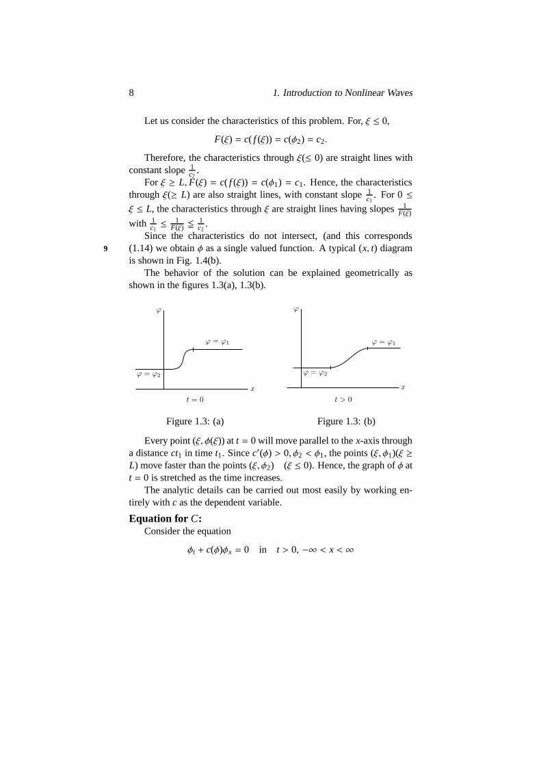
is shown in Fig. 1.4(b).The behavior of the solution can be explained geometricallyas

shown in the figures 1.3(a), 1.3(b).

Figure 1.3: (a) Figure 1.3: (b)

Every point (ξ, φ(ξ)) at t = 0 will move parallel to thex-axis througha distancect1 in time t1. Sincec′(φ) > 0, φ2 < φ1, the points (ξ, φ1)(ξ ≥L) move faster than the points (ξ, φ2) (ξ ≤ 0). Hence, the graph ofφ att = 0 is stretched as the time increases.

The analytic details can be carried out most easily by working en-tirely with c as the dependent variable.

Equation for C:Consider the equation

φt + c(φ)φx = 0 in t > 0, −∞ < x < ∞

1.3. Expansion wave 9

t = 0 : φ = f (x), −∞ < x < ∞.

We have found thatc(φ) is the “propagation speed”, and in con-structing solutions we have to deal with two functions, namely, φ andc.But by multiplying the equation byc′(φ) we obtain

(1.15)Ct +CCx = 0 in t > 0,−∞ < x < ∞,t = 0 : C = F(x),−∞ < x < ∞,

whereC(x, t) = c(φ(x, t)) and 10

F(ξ) = c( f (ξ)).

This equation involves only the unknown functionC(x, t) = c(φ(x, t)); we can recoverφ from C afterwards. The solution of the prob-lem in (1.15) is

(1.16)x = ξ + tF(ξ),

C = F(ξ),

In the special case,

C(x, 0) =

c2 in x ≤ 0,

c2 +c1−c2

L x in 0 ≤ x ≤ L,

c1 in x ≥ L,

thex− t diagram is shown below in Fig. 1.4(b).

O

Figure 1.4: (a)

O

Expansion fan

Figure 1.4: (b)


1.4 Centred expansion wave

We now consider the limiting case of the above problem, asL → 0. Inthe limit the interval [c2, c1] is associated with the origin. In the limit11

we will have the characteristics

x = ξ + tc2, if ξ < 0,

x = ξ + tc1, if ξ > 0,

x = Ct, if ξ = 0, c2 ≤ C ≤ c1.

The collection of characteristicsx = Ct : C ∈ [c2, c1] through theorigin is called a ‘Centred fan’ and we haveC = x/t. In this case thefull solution is

(1.17) C =

c2, if x ≤ c2t,

x/t, if c2t < x < c1t

c1, if x ≥ c1t.

O

Figure 1.5: (a)

O

Centered fan

Figure 1.5: (b)

Thus we have the following.

Theorem.The initial value problem

Ct +CCx = 0, t > 0, −∞ < x < ∞,

1.5. Breaking 11

t = 0 : C =

c2 if ξ < 0,

c1 if ξ > 0,

and C continuous for t> 0, has a unique solution given by(1.17).

1.5 Breaking12

We consider again the geometrical intepretation of the solution of theequations (1.5) and (1.6). We assume thatc′(φ) > 0. The graph ofφ attime t = 0 is the graph off . Since

φ(ξ + tF(ξ), t) = f (ξ),

we find that the point (ξ, f (ξ)) moves parallel tox-axis in the positivedirection through a distancetF(ξ) = ct. It is important to note that thedistance moved depends onξ; this is typical of non-linear phenomena.(In the linear case the curve moves parallel tox-axis with constant ve-locity c0).

O

Figure 1.6:

After some timet = tB, the graph of the curveφ may become manyvalued as shown in the above figure 1.6. This phenomenon is called“breaking”. It could at least make physical sense in the caseof waterwaves (although the equations are in fact not valid), but in most cases athree valued solution would not make sense. We have to reconsider ourapproximations and assumptions.


We have seen that iftF′(ξ) + 1 , 0 then breaking will not occur. A13

necessary and sufficient condition for breaking to occur is thatF′(ξ) < 0for someξ. (We assumec′(φ) > 0). For suchξ′s the envelope of thecharacteristics is obtained by eliminatingξ from the equations

x = ξ + tF(ξ),

0 = tF′(ξ) + 1.

Breaking corresponds to the formation of such an envelope. If weassume thatF′(ξ) is minimum only atξB andF′(ξB) < 0, the first break-ing time will be

tB = −1

F′(ξB)=

1|F′(ξB)|

.

O

(a)

O

(b)

Figure 1.7:

In thex, t, plane the breaking can be seen as follows: sinceF′(ξB) <0, F is a decreasing function in a neighbourhood ofξB will have increas-ing slopes and therefore will converge giving a multivaluedregion.

1.5. Breaking 13

O

Figure 1.8:14

From equations

φt = −F(ξ) f ′(ξ)tF′(ξ) + 1

, φx =f ′(ξ)

tF′(ξ) + 1,

we see thatφt, φx will become infinite at the time of breaking.In order to understand the physical meaning of breaking and meth-

ods used to correct the solution, we need to look at specific physicalproblem.

Probelm on method of characteristics.Solve the following:

1. φt + e−tφx = 0 in t > 0,−∞ < x < ∞,

t = 0 : φ =1

1+ x2

2. φt +C0φx + αφ = 0 in t > 0,−∞ < x < ∞,

t = 0 : φ = f (x)

(α andC0 positive constants)

3. x2φt + φx + tφ = 0 in x > 0,−∞ < t < ∞,

x = 0: φ = Φ(t)

4. Some equation as (3), but regionx > 0, t > 0, 15

t = 0 : φ = f (x), x > 0,

x = 0 : φ = Φ(t), t > 0,


5. φt + φφx + αφ = 0 in t > 0,−∞ < x < ∞,

t = 0 : φ = f (x) as shown in Fig. 1.6.

α is a positive constant.Show that breaking need not always occur; i.e. solution is singleval-

ued for allt in some cases.

Chapter 2

Examples

WE NOW DESCRIBE some problems which lead to the non-linear16

equationφt + c(φ)φx = 0.

In most of the problems we relate two quantities:ρ(x, t) which isthe density of something per unit length andq(x, t) which is the flow perunit time. If the ‘something’ is conserved, then for a section x2 ≤ x ≤ x1

we have the conservation equation

(2.1)ddt

x1∫

x2

ρdx+ q(x1, t) − q(x2, t) = 0.

Figure 2.1:

15

16 2. Examples

If ρ andq are continuously differentiable then in the limitx1 → x2,equation (2.1) becomes

(2.2)∂ρ

∂t+∂q∂x= 0.

If there exists also a functional relationρ = Q(ρ) (this is so to a firstapproximation in many cases) then (2.2) can be written as

(2.3) ρt + c(ρ)ρx = 0,

wherec(ρ) = Q′(ρ).17

We will now give some specific examples.

2.1 Traffic Flow

We consider the flow of cars on a long highway. Hereρ will be thenumber of cars per unit length. Letv be the average local velocity ofthe cars. Thenq, the flow per unit time, is given byq = ρv. For a longsection of highway with no exits or entrances the cars are conserved sothat (2.1) holds. It also seems reasonable to assume that on the averagev is a function ofρ to a first approximation. Henceρ satisfies (2.3). Thevelocity v will be a decreasing functionV(ρ), andQ(ρ) = ρV(ρ). Whenthe density is small the velocity will be some upper limitingvalue, andwhen the density is maximum the velocity will be zero. Therefore thegraph ofV will take a form as shown in the figure 2.2.

O

Figure 2.2:

2.1. Traffic Flow 17

Sinceq = Q(ρ) = ρV, there will be no flow when the velocity ismaximum (i.e.ρ = 0) and whenρ is maximum (i.e.V = 0). Hence the 18

graph ofQ(ρ) will look like the figure 2.3.It was found in one set of observations on U.S. highways that the

maximum density is approximately 225 vehicles per mile (pertrafficlane), and the maximum flow is approximately 1500 vehicles per hour.When the flowq is maximum the density is found to be around 80 vehi-cles per mile.

O

Figure 2.3:

The propagation speed for the wave isc(ρ) = Q′(ρ) = V(ρ) + dVdρ .

SinceV is a decreasing function ofρ, dVdρ < 0. Thusc(ρ) < V(ρ) i.e. the

propagation velocity is less than the average velocity. Relative to indi-vidual cars the waves arrive from ahead.

Referring to theQ(ρ) diagram decreasing in [ρM , ρ j ],Q attains amaximum atρM. Thereforec(ρ) = Q′(ρ) is positive in [0, ρM), zero atρM and negative in (ρM , ρ j ]. That is waves move forward relative to thehighway in [0, ρM), are stationary atρM and move backward in (ρM, ρ j ].

Greenberg in 1959, found a good fit with data for the Lincoln Tunnelin New York by taking

Q(ρ) = aρ log (ρ j/ρ)

with a = 17.2mphandρ j = 228vpm. For this formula, 19

18 2. Examples

V(ρ) =Q(ρ)ρ= a log(ρ j/ρ)

andc(ρ) = Q′(ρ) = a(log(ρ j/ρ) − 1) = V(ρ) − a. Hence the relativepropagation velocity is equal to the constant ‘a’ at all densities and thisrelative speed is about 17 mph. The values ofρM andqmax are:

ρM = 83vpm and qmax = 1430vph(

ρM = ρ j/e and qmax = aρ j/e)

O

(a) (b)

Figure 2.4:

Let f be the initial distribution function as shown in the figure 2.4(a).Sincec′(ρ) = V′(ρ) < 0, breaking occurs on the left. The solution of theproblem is

ρ = ρ(ξ)

x = tF(ξ) + ξ where F(ξ) = c( f (ξ))

Breaking occurs whenF′(ξ) < 0. But

F′(ξ) = c′( f (ξ)). f ′(ξ) < 0 iff f ′(ξ) > 0

i.e. whenf is increasing.In most other examplesc′(ρ) > 0, so that a wave of increasing den-

sity breaks at the front.

2.2. Flood waves in rivers 19

2.2 Flood waves in rivers20

Another example comes from an approximate theory for flood waves inrivers. For simplicity we take a rectangular channel of constant breadth,and assume that the disturbance is roughly the same across the breadth.Then the heighth(x, t) plays the role of ‘density’. Letρ be the flow perunit breadth, per unit time. Then from the conservation law we have

ddt

x1∫

x2

h dx+ q1 − q2 = 0

Taking the limitx2→ x1, we obtain

ht + qx = 0

A functional relationq = Q(h) is a good first approximation when theriver is flooding. Therefore the governing equation is

ht + c(h)hx = 0

wherec(h) = dQdh .

This formula for the wave speed was first proposed by Kleitz andSeddon. The functionQ(h) is determined from a balance between grav-itational acceleration down the sloping bed and frictionaleffects. Whenthe function is given by the Chezy formulaVαh1/2 i.e. V = kh1/2, whereV is the velocity of the flow, we have

Q(h) = Vh= kh3/2

andc(h) = 32kh1/2

=32V. According to this, flood waves move roughly21

half as fast again as the stream.

2.3 Chemical exchange processes

In chemical engineering various processes concern a flow of fluid car-rying some substances or particles through a solid bed. In the process

20 2. Examples

some part of the material in the fluid will be deposited on the solid bed.In a simple formulation we assume that the fluid has constant velocityV. We take density to beρ = ρ f + ρs, whereρ f is the density of thesubstance concerned in the fluid andρs is the density of the materialdeposited on solid bed. The total flow of material across any section is

q = ρ f V.

The conservation equation becomes

(2.4)∂

∂t

(

ρ f + ρs

)

+ V∂ρ f

∂x= 0

To complete the system we require more equations. When the changesare slow we can assume to a first approximation that is a quasi -equi-librium between the amounts in the fluid and on the solid and that thisbalance leads to a functional relationρs = R(ρ f ). Then (2.4) becomes

∂

∂tρ f + c(ρ f )

∂

∂xρ f = 0

where

c(ρ f ) =V

1+ R′(ρ f ).

The relation betweenρ f andρs is discussed in more detail below22

(see 3.6).

2.4 Glaciers

Nye (1960, 1963) has pointed out that the ideas on flood waves applyequally to the study of waves on glaciers and has developed the partic-ular aspects that are most important there. He refers to Finsterwalder(1907) for the first studies of wave motion on glaciers and to indepen-dent formulations by Weertman (1958). For order of magnitude pur-poses, one may take

Q(h) ∝ hN

2.5. Erosion 21

with N roughly in the range 3 to 5. The propagation speed is

c =dQdh= Nv,

wherev is the average velocityQ/h. Thus the waves move about threeto five times faster than the average flow velocity. Typical velocities areof the order of 10 to 100 metres per year.

An interesting question considered by Nye is the effect of periodicaccumulation and evaporation of the ice; depending on the period, thismay refer either to seasonal or climatic changes. To do this,a prescribedsource termf (x, t) is added to the continuity equation; that is one takes

ht + qx = f (x, t), q = Q(h, x).

The consequences are determined from integration of the character-istic equations

dhdt= f (x, t) − Qx(h, x),

dxdt= Qh(h, x).

23

The main results in that parts of the glacier may be very sensitive,and relatively rapid local changes can be triggered by the source term.

2.5 Erosion

Erosion in mountains was studied by Luke. Leth(x, t) be the heightof the mountain from the ground level. It is reasonable to assume afunctional relation betweenht andhx as:

ht = −Q (hx) .

(When the slope of the mountain is greater, it is more vulnerable toerosion).

22 2. Examples

Let

(2.5) s= hx

Then differentiating (2.5) with respect tox we obtain

htx = −Q′ (hx) hxx,

that is∂s∂t+ Q′(s)

∂s∂x= 0, which is our one dimensional non-linear

wave equation withc(s) = Q′(s). When breaking occurs we introducediscontinuities ins, which is hx, andh remains continuous but with asharp corner.

Chapter 3

Shock Waves

WE OBTAINED THE solution of the equation 24

ρt + qx = 0

on the assumptions

(1) ρ andq are continuously differentiable.

(2) There exists a functional relation betweenq and ρ; that is q =Q(ρ).

In our discussions we found the phenomena of breaking in somecases. At the time of breaking we have to reconsider our assumptions.We will approach this in two directions.

(i) We still assume a functional relation betweenq andρ i.e. q =Q(ρ), but allow jump discontinuities forρ andq.

(ii) We assumeρ andq are continuously differentiable andq is a func-tion of ρ andρx. For simplicity we take this in the form

q = Q(ρ) − νρx

whereν > 0.

23

24 3. Shock Waves

3.1 Discontinuous shocks

We now work with the assumption (i). Our conservation equation in theintegrated form:

ddt

x1∫

x2

ρdx+ q1 − q2 = 0

still holds even ifρ andq have jump discontinuities.25

We now assume that the functionρ(x, t) has a jump discontinuity atx = s(t), wheres is a continuously differentiable function oft.

At time t, let x1 > s(t) > x2 andU(t) = s(t) = dsdt . The conservation

equation can now be written as

ddt

s(t)−∫

x2

ρdx+

x1∫

s(t)+

ρe dx

+ q1 − q2 = 0

This implies

s(t)−∫

x2

ρt dx+ s(t)ρ (s(t)−, t) +x1

∫

s(t)+

ρt dx

−s(t)ρ (s(t)+, t) + q(x1, t) − q(x2, t) = 0

Taking the limitsx2→ s(t)− andx1→ s(t)+ we obtain

−s(t)(ρ(s(t)+, t) − ρ(s(t)−, t)) + (q(s(t)+, t) − q(s(t)−, t)) = 0

We symbolically write this as

(3.1) − U[ρ] + [q] = 0

where [.] denotes the jump.Equation (3.1) is called the ‘shock condition’.

The basic problem can now be written as

(3.2)ρt + qx = 0, at points of continuity

− U[ρ] + [q] = 0, at discontinuity points

3.1. Discontinuous shocks 25

There is a nice correspondence between the differential equation andthe shock condition.

∂

∂t↔ −U[.],

∂

∂x↔ [.].

26

The shock condition can also be written as

(3.3) U =q2 − q1

ρ2 − ρ1=

Q(ρ2) − Q(ρ1)ρ2 − ρ1

where the suffixes 1 and 2 stand for the arguments (s(t)+, t) and (s(t)−, t)respectively.

It is important to note that thedirect association of a jump condi-tion with a differential equation in conservation form is not unique. Forexample, consider

(3.4) ρt + ρρx = 0

This can be written asρt + (12ρ

2)x = 0, and the corresponding jumpcondition is

(3.5) − U[ρ] +

[

12ρ2

]

= 0

However, equation (3.4) can also be written as(

12ρ2

)

t+

(

13ρ3

)

x= 0;

the associated shock condition would be

(3.6) − U

[

12ρ2

]

+

[

13ρ3

]

= 0

Obviously (3.5) and (3.6) are different.We have to choose the appropriate jump condition only from the

physical considerations of the problem and the originalintegrated formof the conservation law.

We now give the simplest example in which a shock occurs.

26 3. Shock Waves

Example.The simplest case in which breaking occurs will be 27

ρt + c(ρ)ρx = 0 in t > 0, −∞ < x < ∞,

t = 0 : ρ =

ρ2 if x < 0

ρ1 if x > 0, (ρ2 > ρ1)

with c′(ρ) > 0

O

Figure 3.1:

In this case breaking will occur immediately. The proposed discon-tinuous solution is just a shock moving with velocity

U =Q (ρ2) − Q (ρ1)

ρ2 − ρ1

an separating uniform regionsρ = ρ1 andρ = ρ2 on the two sides.

3.2 Equal area rule

The general question of fitting in a discontinuous shock to replace amultivalued region can be answered elegantly by the following argu-ment. The integrated form of the conservation equation, i.e. ,

ddt

x1∫

x2

ρdx+ q1 − q2 = 0,

3.2. Equal area rule 27

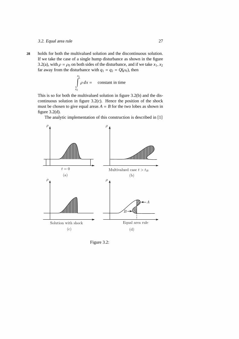
holds for both the multivalued solution and the discontinuous solution.28

If we take the case of a single hump disturbance as shown in thefigure3.2(a), withρ = ρ0 on both sides of the disturbance, and if we takex1, x2

far away from the disturbance withq1 = q2 = Q(ρ0), thenx1

∫

x2

ρdx= constant in time

This is so for both the multivalued solution in figure 3.2(b) and the dis-continuous solution in figure 3.2(c). Hence the position of the shockmust be chosen to give equal areasA = B for the two lobes as shown infigure 3.2(d).

The analytic implementation of this construction is described in [1]

(a) (b)

(c) (d)

Equal area ruleSolution with shock

Figure 3.2:

28 3. Shock Waves

3.3 Asymptotic behavior29

We are interested in finding out what happens to the solution as t → ∞,and this can be obtained directly without going through the previousconstruction in detail. We first study a specialQ(ρ) which simplifies theresults.

The equation is,

(3.7) ρt + qx = 0

with the shock condition

(3.8) − U[ρ] + [q] = 0

If q = Q(ρ) andc(ρ) = Q′(ρ) then, as noted already, (3.7) can bewritten as

Ct +CCx = 0, or Ct +

(

12

C2)

x= 0

whereC(x, t) = c(ρ(x, t)). From the second form of the equation forC, we may be tempted to write the shock condition (3.8) as−U[C] +[ 1

2C2] = 0. But this is not always true, i.e. conservation ofρ does notimply the conservation ofC. However, whenQ is quadratic, say,

Q(ρ) = αρ2+ βρ + γ

then conservation ofρ implies the conservation ofC, sinceC is linear inρ.

This can be easily checked as follows: We have

c(ρ = Q′(ρ) = 2αρ + β;

by equation (3.8),

(3.9) − U[ρ] +[

αρ2+ βρ + γ

]

= 0

30

Now,

3.3. Asymptotic behavior 29

− U[C] +12

[

C2]

= −U[2αρ + β] +

[

2α2ρ2+ 2αβρ +

12β2

]

= 2α

−U[ρ] +[

αρ2+ βρ + γ

]

,

and this is seen to be zero by (3.9). (Here we have used [β] = [ 12β

2] =[γ] = 0 sinceβ andγ are constants).

In this case we can work withC alone and the shock condition is

U =c1 + c2

2

The initial value problem is

(3.10)Ct +CCx = 0, t > 0, −∞ < x < ∞C = F(x), t = 0 : −∞ < x < ∞.

We will now consider the asymptotic behavior of a single hump, i.e.

F(ξ) =

c0 in x ≤ a

g(x) in [a, L]

c0 in x ≥ L

whereg is continuous in [a, L] with g(a) = g(L) = c0, as shown in figure3.2(a).

In this case breaking will occur at the front and we fit a shock toremove multivaluedness. As time increases, much of the initial detailis lost. As this process is continued, it is plausible to reason that theremaining disturbance becomes linear inx. In any event, there is such a31

simple solution withC = x/t. We propose, therefore, that the solution is

(3.11) C =

c0, x ≤ c0txt , c0t ≤ x ≤ s(t),

c0, s(t) < x,

wherex = s(t) is the position of the shock still to be determined.The shock condition isU = c1+c2

2 ; therefore, sincec1 = c0, c2 =

s(t)/t, we have

(3.12)dsdt=

12

c0 +st

30 3. Shock Waves

The solution of this is easily found to be

S = c0t + bt1/2,

whereb is a constant. So we have a triangular wave forC as shown infigure 3.3. The area of the triangle is1

2b2 and this must remain equal tothe areaA under the initial hump. Henceb = (2A)1/2. Only the area ofthe initial wave appears in this final asymptotic solution; all other detailsare lost. It shold be remarked that this behavior is completely differentfrom linear theory.

O

Figure 3.3:

Problems.32

1. Solve(

∂

∂t+ u

∂

∂x

) (

∂

∂t+ u

∂

∂x

)

u+ u = 0, t > 0, −∞ < x < ∞,

t = 0 :

u = 0,

ut = asin kx, −∞ < x < ∞

using the method of characteristics. Find also the time of firstoccurence of singularities.

3.3. Asymptotic behavior 31

2. Solve

ρt + ρρx = 0, t > 0, −∞ < x < ∞,

t = 0 : ρ =

0 in x ≤ 0

x in 0 ≤ x ≤ 12

1− x in 12 ≤ x ≤ 1

0 in x ≧ 1

Find the first time of breaking and the point at which it breaks. Fita shock to this and find the shock velocity.

3. solve

Ct +CCx = 0, t > 0, −∞ < x < ∞,

t = 0 : c =

c0 in x ≦ 0

f (x) in [0, 1]

c0 in x ≥ 1

where f (x) is continuous in [0, 1] with f (0) = f (1) = c0, f de-creases in [0, 1

2] and increases in [12, 1]. Show that breaking oc-

curs. Describe the asymptotic behavior of the solution including 33

the shock.

4. The equation is the same as in the problem 3. Now the initialdistribution is

t = 0 : f =

C0 in x ≦ −1

g(x) in [−1, 1]

C0 in x ≧ 1

whereg is a continuous function withg(0) = g(−1) = g(1) =C0, g is decreasing in [−1, 1

2] and increasing in [−12,

12] and again

decreasing in [12, 1]. Fit shocks wherever necessary and find theasymptotic behavior of the solution. The asymptotic form iscalledan N-wave.

32 3. Shock Waves

5. Solve

Ct +CCx = 0, t > 0, −∞ < x < ∞,

t = 0 : C = F(ξ) = C0 + asin2πξλ

Use the fact thatC = xt is a solution of the equation to describe the

asymptotic behavior of the solution. Deduce that the asymptoticsolution is independent of ‘a’ and that the shock decays liket−1

rather thant1/2. Note that the area under the initial curve in theleft interval [0, λ/2] is not preserved.

6. Assuming that shocks are only required when breaking occursshow that the shock velocity lies betweenC1 andC2.

3.4 Shock structure

In the first approach to resolve breaking we have assumed a functional34

relation inρ andq with appropriate shock conditions. Now we considerthe second approach, namely thatq andρ are continuously differentiablebut thatq is a function ofρ andρx. For simplicity we take

(3.13) q = Q(ρ) − νρx

whereν > 0. (Here the sign ofν is important). Whenρx is small,q = Q(ρ) is a good approximation; but near breaking whereρx is large,(3.13) gives a better approximation. A motivation for (3.13) can be seenfrom traffic flow. In traffic flow, the densityρ is the number of cars perunit length. When the density is increasing ahead,ρx > 0, one expectsthe drivers to adjust the speed a little below equilibriumq = Q(ρ), andwhenρx < 0 perhaps a little above. This is represented by the extra termνρx in (3.13). The other examples in chapter have similar correctionterms in an improved description.

The conservation equation is

ddt

x1∫

x2

ρdx+ q1 − q2 = 0

3.4. Shock structure 33

and for differentiableρ, q we have the differential equation

(3.14) ρt + qx = 0

as before. Using (3.13), (3.14) becomes

(3.15) ρt + c(ρ)ρx = νρxx

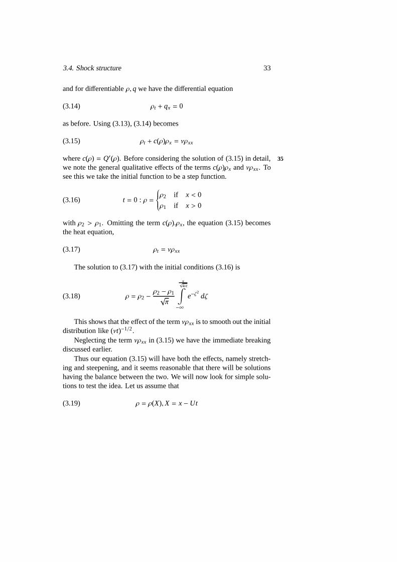
wherec(ρ) = Q′(ρ). Before considering the solution of (3.15) in detail,35

we note the general qualitative effects of the termsc(ρ)ρx andνρxx. Tosee this we take the initial function to be a step function.

(3.16) t = 0 : ρ =

ρ2 if x < 0

ρ1 if x > 0

with ρ2 > ρ1. Omitting the termc(ρ).ρx, the equation (3.15) becomesthe heat equation,

(3.17) ρt = νρxx

The solution to (3.17) with the initial conditions (3.16) is

(3.18) ρ = ρ2 −ρ2 − ρ1√

π

x√4νt

∫

−∞

e−ζ2dζ

This shows that the effect of the termνρxx is to smooth out the initialdistribution like (νt)−1/2.

Neglecting the termνρxx in (3.15) we have the immediate breakingdiscussed earlier.

Thus our equation (3.15) will have both the effects, namely stretch-ing and steepening, and it seems reasonable that there will be solutionshaving the balance between the two. We will now look for simple solu-tions to test the idea. Let us assume that

(3.19) ρ = ρ(X),X = x− Ut

34 3. Shock Waves

is a solution of (3.15), whereU is a constant. We also assume that

(3.20)

ρ→ ρ1 as x→ ∞ρ→ ρ2 as x→ −∞

and ρx → 0 as x→ ±∞

36

Now (3.15) becomes

(3.21) c(ρ)ρX − UρX = νρXX

Using c(ρ) = Q′(ρ) and integrating (3.21) with reference toX weobtain

(3.22) Q(ρ) − Uρ + A = νρX ,

whereA is the constant of integration. Equations (3.22) and (3.20)imply

U =Q(ρ2) − Q(ρ1)

ρ2 − ρ1

which is exactly the same as the shock velocity in the discontinuity the-ory. Equation (3.22) can be written as

1ν=

1Q(ρ) − Uρ + A

·dρdX·

Integrating this with reference toX we get

(3.23)Xν=

∫

dρQ(ρ) − Uρ + A

Sinceρ1, ρ2 are zeroes ofQ(ρ)−Uρ+A the integrals taken over theneighbourhoods ofρ1, ρ2 diverge; soX → ±∞ asρ → ρ1 or ρ2. This isconsistent with our assumptions (3.20).

If c′(ρ) > 0 thenQ(ρ) ≦ Uρ−A in [ρ1, ρ2] and then by (3.22)ρX ≦ 0.Henceρ is decreasing and the solution can be schematically represented37

as in figure 3.4.

3.4. Shock structure 35

O

Figure 3.4:

An explicit solution for (3.15) and (3.16) can be obtained whenQ isthe quadratic

Q = αρ2+ βρ + γ

ThenQ(ρ) − Uρ + A = −α (ρ − ρ1) , (ρ2 − ρ) ,

and by (3.23)

Xν= −

∫

dρα(ρ2 − ρ) (ρ − ρ1)

=1

α (ρ2 − ρ1)log

(

ρ2 − ρρ − ρ1

)

.

Hence we obtain a solution

(3.24) ρ = ρ1 + (ρ2 − ρ1)exp(− (ρ2 − ρ1)αX/ν)

1+ exp(− (ρ2 − ρ1)αX/ν)

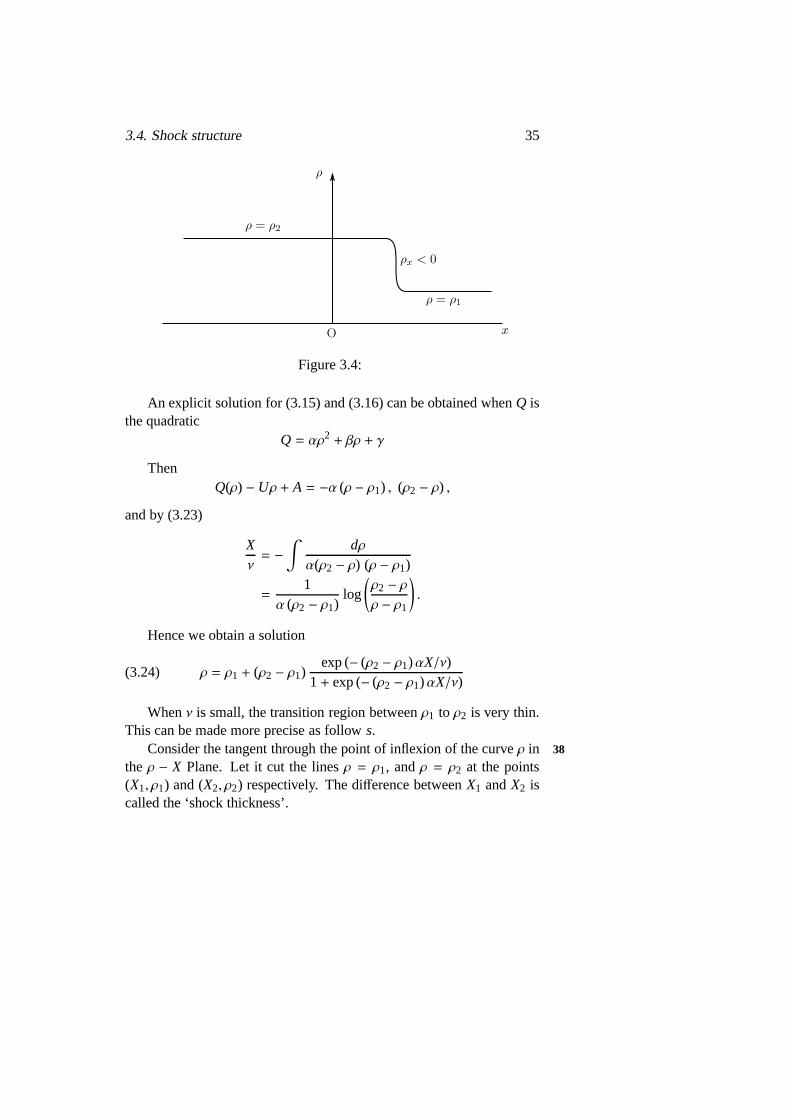
Whenν is small, the transition region betweenρ1 to ρ2 is very thin.This can be made more precise as follows.

Consider the tangent through the point of inflexion of the curveρ in 38

the ρ − X Plane. Let it cut the linesρ = ρ1, andρ = ρ2 at the points(X1, ρ1) and (X2, ρ2) respectively. The difference betweenX1 andX2 iscalled the ‘shock thickness’.

36 3. Shock Waves

O

Figure 3.5:

In the particular case (3.24) we find the shock thickness to be4ν/α(ρ2 − ρ1). From this we conclude that the thickness tends to zero asν tends to zero for fixedρ1, ρ2. However, notice that for fixedν thethickness eventually increases asρ2 − ρ1→ 0.

In the improved theory this smooth, but rapid, transition layer re-places the discontinuous shock of the earlier theory. Similarly, we ex-pect the discontinuities in more general solutions to be replaced by thintransition layers in the improved theory. This can be shown in full detailfor the case of quadraticQ(ρ) as explained in the next section.

3.5 Burger’s equation

Multiplying both sides of the equation (3.15) byc′(ρ) and manipulatingwe obtain

(3.25) Ct +CCx = νCxx + νc′′(ρ)ρ2

x

In the special case whenQ(ρ) is again the quadraticαρ2+βρ+γ we39

havec′′(ρ) = 0. Hence (3.25) becomes

(3.26) Ct +CCx = νCxx

Equation (3.26) is called Burgers’ equation. This equationis origi-nally due to Bateman (1935) but Burgers gave special solutions to it in

3.5. Burger’s equation 37

1940 and emphasized its importance. In 1950–51 Cole and Holfworkedindependently on this and solved it explicitly. They introduced a non-linear transformation which converted (3.26) into the linear heat equa-tion. We now give a brief account of this transformation.

First, if we introduce the variable

(3.27) C = Ψx,

equation (3.26) becomes

Ψxt + Ψx.Ψxx = νΨxxx.

Integrating this with reference tox we obtain

(3.28) Ψt +12Ψ

2x = νΨxx.

The transformation

(3.29) Ψ = −2ν logφ

converts the equation (3.28) into the linear heat equation

(3.30) φt = νφxx

The initial condition

t = 0 : C = F(x)

for (3.26) becomes

(3.31) t = 0 : φ = φ(η) = exp

−12ν

∫

0

F(x) dx

Then the solution of (3.30) with the initial condition (3.31) is 40

φ(x, t) =1√

4πνt

∞∫

−∞

Φ(η) exp

− (x− η)2

4νt

dη

38 3. Shock Waves

and therefore,

C(x, t) =

∞∫

−∞

x−ηt .Φ(η) exp

− (x−η)2

4νt

dη

∞∫

−∞Φ(η) exp

− (x−η)2

4t

dη

The counterparts of the various solutions discussed in the discon-tinuity theory can be studied in this improved theory. Except for ex-tremely weak shocks in certain cases, the only significant change (forsmallν) is the smoothing of the shocks into thin transition layers.A fullaccount is given in [1].

3.6 Chemical exchange processes; Thomas’s equa-tion

The situation is similar in chemical exchange processes. The conserva-tion equation is

(3.32)∂

∂t

(

ρ f + ρs

)

+∂

∂x

(

Vρ f

)

= 0

whereρ f , ρs are as before (see section 2.3. We took

(3.33) ρs = R(

ρ f

)

to be an approximation and obtained the one dimensional non-linearwave equation. In many cases a more detailed description forthe secondrelation betweenρ f andρs is

(3.34)∂ρs

∂t= K1 (A− ρs) ρ f − K2ρs

(

B− ρ f

)

whereK1,K2,A, B are constants.A, B represent the saturation levels of41

the substance in the solid bed and the fluid respectively.An approximation of the form (3.33) is obtained from (3.34) by ne-

glecting the term∂ρs∂t . We will work with the ‘improved theory’ provided

by (3.34).

3.6. Chemical exchange processes; Thomas’s equation 39

Thomas (1945) gave transformations to convert (3.32) into alinearequation.

Step 1.By the transformation

(3.35) τ = t −xV, σ =

xV

(3.32) and (3.34) become

∂ρ f

∂σ+∂ρs

∂τ= 0(3.36)

and∂ρs

∂τ= αρ f − βρs − γρsρ f(3.37)

whereα, β, γ are constants.

Step 2.Consider now the transformation

(3.38) ρ f = Ψτ, ρs = −Ψσ

Then (3.36) is satisfied identically, and (3.37) becomes

(3.39) Ψστ + αΨτ + βΨσ + γΨσ.Ψτ = 0

Step 3.The final step is to introduce the transformation

(3.40) Ψ =lγ

logχ,

and this is the crucial one. Then (3.39) reduces to 42

(3.41) χστ + αχτ + βχσ = 0

which is linear and can be solved by standard methods. Again variousquestions in the discontinuity theory can be viewed from theimproveddescription.

Chapter 4

A Second Order System;Shallow Water Waves

43

THE EXTENSION OF the ideas presented so far to higher order sys-tems can be adequately explained on a typical example. We shall usethe so called shallow water wave theory for this purpose, although thepioneering work was originally done in gas dynamics.

4.1 The equations of shallow water theory

In shallow water theory the heighth(x, t) of the water surface above thebottom is small relative to the typical wave lengths; it is called shallowwater theory or long wave theory depending on which aspects one wantsto stress.

We take the bottom to be horizontal and neglect friction. Letthedensity of the water be normalized to unity and let the width be oneunit.

Let u(x, t) be the velocity,p0 the atmospheric pressure and (p0 +

p′(x, t)) the pressure in the fluid. In every sectionx2 ≦ x ≦ x1 the mass

41

42 4. A Second Order System; Shallow Water Waves

is conserved, i.e.

ddt

x1∫

x2

h(x, t) dx+ q1 − q2 = 0,

where the flowq = uh.

Figure 4.1:

44

Taking the limitx2→ x1, we obtain

ht + qx = 0,

i.e. ht + (uh)x = 0(4.1)

This time a second relation betweenu andh is obtained from theconservation of the momentum in thex-direction. If we consider a sec-tion x2 ≦ x ≦ x1, as shown in figure 4.1, a constant pressurep0 act-ing all around the boundary, including free surface and bottom, is self-equilibrating. Therefore, only the excess pressurep′ contributes to themomentum balance. IfP(x, t) denotes the total excess pressure,

P =

h∫

0

p′ dy

4.1. The equations of shallow water theory 43

acting across a vertical section, the momentum equation is then

(4.2)ddt

x1∫

x2

hu dx= hu2 |x=x2 −hu2 |x=x1 +P2 − P1

wherePi = P (xi , t) , i = 1, 2.The term in the left hand side of (4.2) is the total rate of change

of momentum in the sectionx2 ≦ x ≦ x1, andhu2 |x=xi , on the right, 45

denotes the momentum transport across the surface throughx = xi(i =1, 2).

The basic assumption is shallow water theory is that the pressure ishydrostatic, i.e.

(4.3)∂p∂y= −g

whereg is the acceleration due to gravity.Integrating (4.3) and assuming the conditionp = p0 at the topy = h,

we obtainp = p0 + g(h− y).

Hence the total excess pressure is

(4.4) P =

h∫

0

g(h− y) dy=12

gh2

Equations (4.2) and (4.4) yield

(4.5)ddt

x1∫

x2

hu dx+

[

hu2+

12

gh2]x1

x2

= 0

The conservation form should be noted.In the case of river flow discussed earlier, there would also be further

terms on the right hand side of (4.5) due to the slope effect and friction;the slope is now omitted and frictional effects are neglected.


In the limit x2→ x1, (4.5) becomes

(4.6) (hu)t +

(

hu2+

12

gh2)

x= 0

Equations (4.1) and (4.6) provide the system for the determination ofuandh.

If h and u have jump discontinuities, the shock conditions corre-46

sponding to (4.1) and (4.6) (but deduced basically from the original in-tegrated form) are

− U[h] + [uh] = 0

− U[uh] +

[

hu2+

12

gh2]

= 0

respectively, whereU is the shock velocity.Using equations (4.1) in (4.6) we obtain

(4.7) ut + uux + ghx = 0;

equation (4.1) can be written as

(4.8) ht + uhx + hux = 0

4.2 Simple waves

Each of the conservation equations (4.1) and (4.6) takes ourearlier form

ρt + qx = 0.

In those earlier cases, a relationq = Q(ρ) was provided in the ba-sic formulation. In the present case, we might ask in relation to (4.1)whether there are solutions in whichq = uh is a function ofh, wherethe appropriate functional relation is provided not from outside obser-vations but from the second equation (4.6). We might equallywell askwith respect to (4.6) whether there are solutions in whichhu2

+12 gh2 is

a function ofhu, where the functional relation is provided by (4.1). The

4.2. Simple waves 45

two are equivalent and come down to the question of whether there aresolutions in which, say,h is a function ofu. We try

h = H(u),

and consider the consistancy of the two equations. We use thesimplified 47

equations (4.7) and (4.8) for the actual substitution. (This approach isequivalent to Earnshaw’s approach in gasd-namics).

After the substitutionh = H(u), we have

ut + uux + gH′(u)ux = 0(4.7)′

ut + uux +H(u)H′(u)

ux = 0(4.8)′

For consistancy we require (4.8)′

gH′(u) =H(u)H′(u)

,

which implies

(4.9)√

gH′(u) = ±√

H

Taking the positive sign in (4.9) and integrating we obtain

(4.10) 2√

gH − 2√

gH0 = u

whereH0 = H(0). Then (4.7)′ becomes

(4.11) ut +(

u+√

gH)

ux = 0

Thusu +√

gH is the velocity of propagation. If we use (4.10) andsetc0 =

√gH0, equation (4.11) can be written as

(4.12) ut +

(

c0 +3u2

)

ux = 0

We now have exactly the form discussed in the earlier chapters andcan take over the results from there. Equation (4.10) is the functionalrelation equivalent toq = Q(ρ).


If we take the negative sign in (4.9) we will obtain the relation

2√

gH − 2√

gH0 = −u

and the equation 48

ut +(

u−√

gH)

ux = 0

Each of these equations represents a so called ‘simple wave’. Thechoice of signs in (4.10) and (4.12) correspond to wave moving to theright, the other signs correspond to one moving to the left.

Example .We consider a piston ‘wave maker’ moving parallel to thex-axis in the negative direction with given velocity. Initially when thepiston is at rest, the water is at rest.

Figure 4.2:

The movement of the piston is represented in thex, t plane by thecurve

x = X(t), u = X(t),

whereX(t) is a given function.

4.2. Simple waves 47

Figure 4.3:

The flow of water is governed by the equation 49

ut +

(

c0 +3u2

)

ux = 0,

since a wave moving to the right is produced.Following the constructions of chapter 1, we choose a characteristic

curve on whichdxdt= c0 +

3u2.

On this characteristicdudt = 0; therefore,u = constant= X(τ), if the

characteristic is passing through (X(τ), τ). Therefore,dxdt = c0 +

32X(τ).

Integrating we obtain

x = X(τ) +

c0 +32

X(τ)

(t − τ).

Hence the solution of the piston problem is

x = X(τ) +

c0 +32

X(τ)

(t − τ),

u = X(τ),

whereτ is the characteristic parameter.As in the previous cases, expansion waves (in this caseX(t) ≦ 0) do

not break and the solution is valid for allt. On the other hand, moving


the piston forward or providing a positive acceleration, will produce abreaking wave. The inclusion of discontinuities based on the jump con-ditions (noted after equation (4.6)) is similar in spirit tothe discussion ofchapter 3, but is somewhat more complicated than before. Therelation(4.10) is not strictly valid across discontinuities (note it was deducedfrom the differential equations), and approximations have to be made50

if the simple wave solutions are still used. (See [1] for details in theequivalent gas dynamics case).

4.3 Method of characteristics for a system

The above simple wave solutions provide an interesting approach andtie the discussion closely to the earlier material on a single equation.However, they are limited to waves moving in one direction only. Wewant to consider questions of waves moving in both directions and in-teracting with each other. We shall also find via Riemann’s arguments afurther understanding of the role of the simple waves.

Since we already know thatc =√

gh is a useful quantity here, weshall introduce it at the outset to simplify the expressionsbut it is in noway crucial. The equations (4.7) and (4.8) then become

ut + uux + 2ccx = 0,(4.13)

ct + ucx +12

cux = 0.(4.14)

Now we note that each equation relates the directional derivativesof u andc for different directions. If the directions were the same wemight make progress as in Chapter 1. But we can try linear combinationsof (4.13) and (4.14) that have the desired property. Accordingly, weconsider (4.13)+m. (4.14), wherem is a quantity to be determined. Wehave

(4.15) ut + uux + 2ccx +m

ct + ucx +12

cux

= 0

51

4.3. Method of characteristics for a system 49

This will take the desired form,

ut + vux +mct + vcx = 0,

provided

u+m2

c = u+2cm= v.

The latter givesm= ±2. Puttingm= 2 in (4.15) we have

(4.16) (u+ 2c)t + (u+ c) (u+ 2c)x = 0

We choose theC+ characteristic to be

C+ :dxdt= u+ c

OnC+, (4.16) becomes,ddt(u+ 2c) = 0, which impliesu+ 2c = constantonC+.

Takingm= −2 in (4.15), we obtain

(4.17) (u− 2c)t + (u− c) (u− 2c)x = 0

we choose theC− characteristic with the property

C− :dxdt= u− c

Then equation (4.17) implies:

On C−,ddt

(u− 2c) = 0,

i.e. u− 2c = constant on C−

Thus we obtian

u+ 2c = constant ondxdt= u+ c

u− 2c = constant ondxdt= u− c

The constants may differ from characteristic to characteristic.


This is the method of characteristics for higher order systems. For 52

annth order system of first order equations foru1, . . . , un, one looks fora linear combination of the equations so that the directional derivativesof eachui is the same. If there aren real different combinations with thecharacteristic property the system ishyperbolic.

In the present case the characteristic equations will be useful in var-ious ways. We first reconsider the simple wave solutions.

4.4 Riemann’s argument for simple waves

We focus on the piston problem to show how the argument goes throughand refer to figure 4.4.

O

Figure 4.4:

Using the fact thatu− c ≦ u we can show that theC− characteristicscover the whole region(x, t) : t ≧ 0, x ≧ X(t). On eachC− we haveu− 2c = constant; from the initial condition

t = 0 : u = 0, c = c0,

we find thatu − 2c = −2c0. But this is true for eachC− with thesame53

constant. Therefore

(4.18) u− 2c = −2c0

4.5. Hodograph transformation 51

everywhere. This is exactly the relation (4.10): We could now referto the previous discussion to complete the solution. To complete thesolution in the present context, we use theC+ relation

u+ 2c = constant ondxdt= u+ c

From (4.18) this becomes

u = constant ondxdt= co +

32

u,

exactly the information contained in (4.12). We conclude that

(4.19)

u = X(τ)

x = X(τ) +

c0 +32

X(τ)

(t − τ)

as before.

Problem. Dam break. In an idealization, the flow of water out of a damis governed by the equations

ut + uux + 2ccx = 0

ct + ucx +12

cux = 0

with the initial conditions

t = 0 :

u = 0, −∞ < x < ∞,

h =

h1, −∞ < x < 0,

0, 0 < x < ∞.

Find the solution. (There is no discontinuity and the final answertakes a simple explicit form).


4.5 Hodograph transformation54

In the interaction of waves, where both families of characteristics carrynontrivial disturbances (i.e. (4.18) does not hold), solutions are muchmore difficult, and numerical methods are often used.

However, one alternative analytic method for studying the interac-tion of waves, or the two interacting families of waves produced by gen-eral initial conditions, is the ‘hodograph’ method. The equations are

(4.20)ct + ucx +

12

cux = 0

ut + uux + 2ccx = 0

and we note that the coefficients are functions of the dependent vari-ables only. We try to make use of that fact by interchanging the role ofdependent and independent variables.

We haveu = u(x, t), c = c(x, t) and consider the inverse functions

x = x(u, c), t = t(u, c).

The term ‘hodograph’ is used when the velocitiesu andc are con-sidered as independent variables. We have the relations

ct = −xu

g, cx =

tug,

ut =xc

g, ux = −

tcg,

whereg = (c,t)(u,c) = xutc − xctu.

For the system (4.20), the highly non-linear factorg cancels through55

and we have

(4.20)′xu = utu −

12

ctc

xc = utc − 2ctu

Notice g would not cancel if there were undifferentiated terms.Equations (4.20)′ are now linear and this offers considerable simplifi-cation.

4.5. Hodograph transformation 53

Differentiating the first equation in (4.20)′ with respect toc, par-tially, and the second one with respect tou and subtracting, we find

(4.21) 4tuu = tcc+3c

tc.

This is a linear equation fort(u, c) which can be solved by standardmethods.

However, the difficulties in this method are:

(1) The transformed boundary conditions in theu−c plane will some-times be awkward.

(2) When breaking occursg = 0, corresponding to the multivalued-ness, and fitting in shocks may sometimes be difficult in this plane.

For these reasons a numerical method is often preferred. However, inthe case of waves on a sloping beach an analogous method has led to anextremely valuable solution; it will be described in section 5.4.

In that connection, a particularly elegant form of the transformationis useful and we note it here for the case of the horizontal bottom. We 56

use the characteristic form

p = u+ 2c = constant ondxdt= u+ c

q = u− 2c = constant ondxdt= u− c.

If p, q are used as variables, we can write

dxdt= u+ c

as xq = (u+ c)tq,

sincep is a constant on that characteristic andq can be used as parame-ter. Similarly

xp = (u− c)tp.

We then substitute foru andc in terms ofp andq to obtain

xq =3p+ q

4tq, xp =

p+ 3q4

tp


These are the linear hodograph equations equivalent to (4.20)′. Elimi-natingx, we have

2(q− p)tpq − 3(

tq − tp

)

= 0,

which is equivalent to (4.21).

Chapter 5

Waves on a Sloping Beach;Shallow Water Theory

IN THE LAST chapter we considered flow over a horizontal levelsur- 57

face. In the case of a non-uniform bottom, we will get an additionalterm in the horizontal momentum equation due to the force acting onthe bottom surface.

5.1 Shallow water equations

We choose a coordinate systemx, y such thaty = −h0(x) denotes thebottom andy = η(x, t) the water surface. Hence the total depthh(x, t) is

h(x, t) = h0(x) + η(x, t).

The equation of conservation of mass is

(5.1)ddt

x1∫

x2

h(x, t) dx+ [uh]x1x2= 0

as before, and ifu andh are continuously differentiable, then

(5.1)′ ht + (uh)x = 0.

55

56 5. Waves on a Sloping Beach; Shallow Water Theory

O

Figure 5.1:

Let us now consider the momentum balance in thex-direction. Let58

p′ be the excess pressure as before. When the bottom is not horizontal,the contribution ofp′ from the bottom surface will have a non-zero hor-izontal component. Let us consider a thin section of thicknessdx andlet ds be the line element along the bottomy = −h0(x). Let α be theinclination ofds to thex-axis. Then

ds=dx

cosα.

Hence the momentum balance in the horizontal direction is

(5.2)ddt

x1∫

x2

hu dx+

[

hu2+

12

gh2]x1

x2

= −x1

∫

x2

(

p′dx

cosα

)

sinα

In the shallow water theory we havep′ = g(η − y). At y = −h0, p′ =g(η + h0) = gh. Therefore (5.2) becomes

(5.3)ddt

x1∫

x2

hu dx+

[

hu2+

12

gh2]x1

x2

=

x1∫

x2

ghdh0

dxdx,

sincedh0dx = tanα. If all the quantities are smooth, in the limitx2 → x1,

we obtain

(5.4) (hu)t +

(

hu2+

12

gh2)

x= gh

dh0

dx

5.2. Linearized equations 57

When there are discontinuities, the shock condition derived from(5.3) is

−U[hu] +

[

hu2+

12

gh2]

= 0,

since the right hand side of (5.3) becomes zero in the limitx2 → x1.Thus, the shock conditions are unaffected by the extra termghdh0

dx dueto the non-uniform bottom.

Using the mass conservation equation (5.1)′ the momentum equa-59

tion (5.4) can be written as

ut + uux + gηx = 0.

Hence the system of equations for the flow of shallow water over anon-uniform bottom is

(5.5)

ht + uhx + hux = 0,

ut + uux + gηx = 0,

h = h0 + η.

5.2 Linearized equations

We assume that the disturbances are small of orderǫ ≪ 1 i.e. η

h0= 0(ǫ)

and u√gh0= o(ǫ). We also assume that the derivative are also of the

same order.Sinceh = η(x, t) + h0(x), equations (5.5) can be written down as

ηt + uh′0 + h0ux + uηx + ηux = 0(5.6)

ut + uux + gηx = 0.(5.7)

The first three terms of (5.6) are of order 0(ǫ) whereas the last twoterms are of order 0(ǫ2). In the equation (5.7)uux = 0(ǫ2) and the otherterms are of orderǫ. Hence to a first order approximation we have

(5.8)ηt + h0ux + h′0u = 0,

ut + gηx = 0.


Equations (5.8) are the linearized versions of equations (5.5). Differ-entiating the first equation of (5.8) partially w.r.t.t and using the second60

equation, we obtain

(5.9) ηtt = gh0ηxx + gh′0ηx.

This is the wave equation with an additional term. Ifh0 were con-stant then

ηtt = gh0ηxx

and the general solution of this is

η = f1(

x−√

gh0t)

+ f2(

x−√

gh0t)

.

The velocity of propagation is√

gh0.

5.3 Linear theory for waves on a sloping beach

We now consider a sloping beach with inclinationβ to the horizontal.We assumeβ to be small so that linearized shallow water theory can beapplied.

However there will be some questions about validity to be consid-ered later. These are

(i) The question of using the shallow water theory asx→ ∞, whenthe water becomes deep.

(ii) The question of the assumptionη/h0 ≪ 1 nearx = 0 whereh0→0.

We have to solve equation (5.9) withh0 = x tanβ and we takeh0 ≃βx sinceβ is very small. Hence the equation can be written as

(5.10) ηtt = gβxηxx + gβηx.

Let η = N(x)e−iωt be a solution of equation (5.10). Then we obtain61

an ordinary differential equation forN as follows:

(5.11) N′′ +1x

N′ +ω2

gβ1x

N = 0.

5.3. Linear theory for waves on a sloping beach 59

This is to be solved in 0< x < ∞.The pointx = 0 is a regular point of equation (5.11), andx = ∞ is

an irregular point. This suggests a transformation to Bessel’s equationor some other confluent hypergeometric equation. In fact thetransfor-mation

x =gβ

ω2

X2

4converts it into the Bessel equation of order zero.

(5.12)d2N

dX2+

lX

dNdX+ N = 0.

The Bessel functionsJ0(X),Y0(X) are two linearly independent so-lutions of the equation (5.12). Hence a general solution of (5.11) is

N = AJ0

(

2ω√

xgβ

)

− iBY0

(

2ω√

xgβ

)

,

whereA andB are constants. Since the power series forJ0(X) contains

only even powers ofX, J0

(

2ω√

xgβ

)

is an integer power series inx and is

regular at the beachx = 0. We note thatY0 has a logarithmic singularityat x = 0.

The complete solution of (5.10) is

η(x, t) =

AJ0

(

2ω√

xgβ

)

− iBY0

(

2ω√

xgβ

)

e−iωt.

As x→ ∞ the asymptotic formula forη is

(5.13)

η ∼ 1√π

( gβ

ω2x

)1/4 A+ B2

exp

(

−i2ω√

xgβ− iωt +

πi4

)

+A− B

2exp

(

i2ω√

xgβ− iωt −

πi4

)

.

62

The first term in the bracket corresponds to an incoming wave andthe second one to an outgoing wave. In a uniform medium an outgoingperiodic wave is given by

aeiκx−iωt ,


whereκ, ω, a are the wave number, frequency and amplitude respec-tively. The terms in (5.13) are generalizations to the form

a(x, t)eiθ(x,t) .

A generalized wave number and frequency can be defined in termsof the phase functionθ(x, t) by

(5.14) κ(x, t) = θx, ν(x, t) = −θt;

the generalized phase velocity is

(5.15) c(x, t) =ν

k= −

θt

θx.

The functiona(x, t) is the amplitude.In our particular case the outgoing wave has

θ(x, t) = 2ω√

xgβ− ωt −

π

4.

Hence the wave number, frequency and phase velocity are

κ(x, t) = θx =ω√

gβx,

ν(x, t) = −θt = ω,

c(x, t) =√

gβx.

We note that the waves get shorter asx→ 0, and thatc =√

gh0(x)is the generalization of the result for constant depth. The incoming wave63

is similar with the opposite sign of propagation.

Behavior asx→ ∞ .We note that the amplitude a varies proportional tox−1/4. As x →

∞, a → 0. This means that, within shallow water, we cannot pose thenatural problem of a prescribed incoming wave at infinity with a given

5.3. Linear theory for waves on a sloping beach 61

nonzero amplitude. This is due to the failure of the shallow water as-sumptions at∞, one of the questions noted at the beginning of this sec-tion. It it found from the full theory in Chapter 7, (for the solution cor-responding toJ0) that the ratio of amplitude at infinitya∞ to amplitudeat shorelinea0 is in fact (2β/π)1/2. Therefore,a∞/a0→ 0 asβ→ 0, andthe x−1/4 behavior is the shallow water theory’s somewhat inadequateattempt to cope with this. However, the full solution does show that theshallow water theory is a good approximation near the shore.And it isvaluable there since, for example, the corresponding nonlinear solutioncan be found in the shallow water theory (see the next section) but notin the full theory.

Behavior asx→ 0 and breaking .We see from (5.13) that the ratio ofB to A, which controls the

amount ofJ0 andY0 in the solution, also determines the proportion ofincoming wave that is reflected back to infinity.

For B = 0, we have perfect reflection with 64

(5.16) η = AJ0

(

2ω

√x

gβ

)

e−iωt

and the solution is bounded and regular at the shorelinex = 0.In the other extreme,A = B, there is no reflection, we have a purely

incoming wave

(5.17) η = A (J0 − iY0) e−iωt,

but it is now singular at the shoreline. The interpretation of the singular-ity is that it is the linear theory’s crude attempt to represent the breakingof waves and the associated loss of energy. AsB increases, more energygoes into the singularity (breaking) and less is reflected.

Although breaking is the most obvious phenomenon we observeatthe seashore, a number of long wave phenomena (long swells, edgewaves, tsunamis) are in the range where breaking does not occur so thatthe J0 solution (B = 0) with perfect reflection is relevant. This is for-tunate since practical use of theY0 solution would be limited, althoughthe situation is mathematically interesting.


The singular solution is related also to the second questionnotedat the beginning of this section: The breakdown of the linearizing as-sumptionη/h0 ≪ 1 ash0 → 0 at the shoreline. On this we can saythat the nonlinear solution corresponding toJ0 can be found withoutthis assumption (next section), and it endorses the linear approximation.TheY0 solution with its crucial ties to complicated nonlinear breaking65

is clearly a different matter.

The eigenvalue problem and expansion theorem.One further aspect of theY0 solution is certainly intriguing mathe-

matically. The eigenvalue problem (5.11) withω2/gβ as eigenparameteris of “limit circle” type at x = 0. This is identified by the fact thatbothsolutions are square integrable there and it has important remificationsin the general theory of eigenfunction expansions. The mainone is thatvarious choices of linear combinations ofJ0 andY0 each lead to a sat-isfactory eigenfunction expansion to represent a given square integrablefunction (as required, say, in solving the initial value problem). In ourcontext this is interpreted as an arbitrary choice of the degree of break-ing, within this theory. The natural choice would then appear to be anexpansion theorem

(5.18) f (x) =

∞∫

0

A(ω)

J0

(

2ω√

xgβ

)

− imY0

(

2ω√

xgβ

)

dω

wherewe must givem in the range 0≤ m≤ 1 to indicate our estimate ofthe relative amount of breaking. With the choicem= 0 this is the usualFourier-Bessel expansion, and is certainly one valid possibility. Whenm, 0, the result obtainde from the usual general theory (see Titchmarsh[2], p. 78) is not quite (5.18). TheY0 has to be replaced by

(5.19) Y0

(

2ω√

xgβ

)

− 2π

J0

(

2ω√

xgβ

)

logω.

66

It seems hard to find a “natural” physical interpretation forthis mod-ification. Moreover, one may still ask whether the unmodifiedform

5.4. Nonlinear waves on a sloping beach 63

(5.18) is in fact a correct possible choice. A further question that arises,since we expect different amounts of breaking for different frequencies,is whether there is an expansion theorem for reasonable choices offunc-tions m(ω) in (5.18).

It might be remarked that these points are particularly interestingbecause in most applications where the “limit circle” case arises, onlya bounded solution makes physical sense and the one parameter arbi-trariness is not in fact used in any significant way. The niceties of themathematical discussion are not displayed.

Tidal estuary problem .In a channel where the breadthb(x) varies, as well as the depthh0(x),

the shallow water equations are modified to

∂

∂t(h0 + η) b + ∂

∂x(h0 + η) ub = 0,

∂u∂t+ u

∂u∂x+ g

∂η

∂x= 0.

For the caseh0(x) = βx, b(x) = αx the linearized equation forη canagain be solved in Bessel functions. G.I. Taylor used this solution tostudy the large tidal variations in the Bristol channel. In this applica-tion to extremely long waves, breaking is not an issue and only the Jn

solution is accepted.

5.4 Nonlinear waves on a sloping beach67

In Section 5.3 we considered the linear approximation of theequationsfor waves on a sloping beach. Carrier and Greenspan [4] in 1958 gavean exact solution of the nonlinear equations using a modifiedtype ofhodograph transformation applied to characteristic variables. We recallthat the governing equations are

ht + uhx + hux = 0,

ut + uux + ghx − gβ = 0,


whereh = βx+ η(x, t).Introducing the variablec =

√

gh, which we know to be significant,the above equations become

(5.20)2ct + 2ucx + cux = 0,

ut + uux + 2ccx − gβ = 0.

Due to the presence of the termgβ, the straight forward hodographtransformation (u, c) → (x, t) will not simplify the equations, sincethis time the Jacobiang would not cancel through. However, Carrierand Greenspan introduced new variables suggested by the characteristicforms and applied a hodograph transformation to these.

The characteristic forms of the equations (5.20) are

(u+ 2c)t + (u+ c) (u+ 2c)x − gβ = 0,

(u− 2c)t + (u− c) (u− 2c)x − gβ = 0.

These can be written as68

(u+ 2c− gβt)t + (u+ c) (u+ 2c− gβt)x = 0,

(u− 2c− gβt)t + (u− c) (u− 2c− gβt)x = 0.

TheC+ andC− characteristic curves are defined by

(5.21)C+ :

dxdt= u+ c, u+ 2c− gβt = constant,

C− :dxdt= u− c, u− 2c− gβt = constant.

We define the characteristic variablesp, q by

p = u+ 2c− gβt,(5.22)

q = u− 2c− gβt.(5.23)

Then equations (5.21) can be written

xq = (u+ c)tq,

xp = (u− c)tp,


which introduces the hodograph transformation (p, q) → (x, t). Solv-ing (5.22), (5.23) foru, c and inserting them in the above equations weobtain

(5.24)xq =

(

3p+ q4+ gβt

)

tq,

xp =

(

p+ 3q4+ gβt

)

tp.

Equations (5.24) are still nonlinear, but by good fortune the nonlin-ear terms are in the form (1

2gβt2)q, (12gβt2)p so that when we take cross

derivatives and subtract to obtain an equation fort, these terms can-cel each other. This was the remarkable fact observed by Carrier andGreenspan. Differentiating the first equation in (5.24) partially with re-spect top and the second equation with respect toq and subtracting we69

obtain

(5.25) 2(p− q)tpq + 3(

tq − tp

)

= 0.

Equation (5.25) is alinear equation which can ve solved by standardmethods.

This is the main step, but further transformations can be used toconvert (5.25) into the cylindrical wave equation whose solutions arealready well documented. First, by the transformation

(5.26)σ = p− q,

λ = −(p+ q),

equation (5.25) becomes

(5.27) tλλ = tσσ +3σ

tσ.

This can be further simplified by introducing the transformation

(5.28) gβt =λ

2− φσσ

;


the term−φσσ

is for transforming (5.27) into the cylindrical wave equa-tion and the termλ2 is included to give a simple final form foru. Thuswe obtain cylindrical wave equation

(5.29) φλλ = φσσ +1σφσ

Equations (5.22), (5.23) giveu, c in terms ofp, q. From the trans-formation (5.26) we obtainp, q in terms ofσ, λ. These together withequation (5.28) lead to

c =σ

4(5.30)

u = −φσ

σ,(5.31)

gβt =λ

2− φσσ.(5.32)

It can be shown from (5.24), with a use of (5.29), that70

(gβx)σ =

(

−14φλ +

12φ2σ

σ2+σ2

16

)

σ

,

(gβx)λ =

(

−14φλ +

12φ2σ

σ2

)

λ

.

From these we obtain

(5.33) gβx = −14φλ +

12

φ2σ

σ2+σ2

16.

The final set of transformations (5.30)-(5.33) is sufficiently involvedthat it seems inconceivable that anyone would discover themdirectly.One can note that

u− gβt = −λ2

and12

u2+ c2 − gβx = +

14φλ

take simple forms and these combinations appear in two alternativeways of absorbinggβ in conservation forms for the second of (5.20),i.e.

(u− gβt)t)t +

(

12

u2+ c2

)

x= 0,


ut +

(

12

u2+ c2 − gβx

)

x= 0.

But this comment does not appear to lead any further.Almost equally important as the linearity of (5.29) is the fact that the

moving shorelinec = 0 is now fixed atσ = 0 in the new independentvariables. We can now work in a fixed domain.

The simplest separable solution of (5.29) is

(5.34) φ = N(σ) cosαλ,

whereα is an arbitrary separation constant. The equation forN(σ) isthen the Bessel equation of order zero.

(5.35) N′′ +1σ

N′ + α2N = 0.

The solution bounded at the shorelineσ = 0 is 71

N = AJ0(ασ),

whereA is a constant. Hence

(5.36) φ = AJ0(ασ) cosαλ.

Equation (5.36) together with the above transformations and rela-tions give an exact solution for the non linear equation (5.20).

Linear approximation .It will be useful to note how the linearized approximation isobtained

from (5.36). In the linear theoryu is small which impliesφ is small.Hence to a first order approximation we obtain from (5.32), (5.33) that

(5.37)gβt ≃

λ

2,

gβx ≃ σ2

16.

Thusφ ≃ AJ0

(

4α√

gβx)

cos(2αgβt).


Takingα = ω2gβ we obtain

φ ≃ AJ0

(

2ω√

xgβ

)

cosωt

which is in agreement with our result obtained in section 5.3. To relateφ to the particle velocityu and elevationη, we first note that

u = −φσ

σ= −α2A

J′0(ασ)

ασcosαλ

≃2ωa0

β

J′0

(

2ω√

xgβ

)

2ω√

xgβ

cosωt,

where72

(5.38) a0 =β

2ωα2A =

ω

8gβ2A.

Then rather than trying to improve on the approximation forσ andhencec to findη, we rather note that the above linearized approximationfor u goes along in linear theory with

(5.39) η = −a0J0

(

2ω√

xgβ

)

sinωt.

These approximations provide a rough way to interpret the variablesin the nonlinear form (5.36). In particular we see it as the nonlinearcounterpart of the wave with perfect reflection at the beach.

Run-up. Perhaps the most important quantity among the results is therange ofx at the shorelineσ = 0, since this provides the amplitude ofthe run-up.If x = F(λ, σ) then the range ofx atσ = 0 is [min

λF(λ, 0),max

λF(λ, 0)].

Using (5.33), (5.36) and the fact that limz→0

J′0(z)z = −

12 we obtain:

at the shore σ = 0, gβx =14αAsinαλ +

18α4A2 cos2αλ.


At maximum or minimum run-up,u = −φσ/σ = 0. Therefore, from(5.36),

cosαλ = 0, and hence sinαλ = ±1.

Therefore at the maximum run up:gβx = 14αA, at the minimum run

up: gβx = −14αA. Hence the range ofx is

−αA4gβ≤ x ≤

αA4gβ

.

73

If a0 is the vertical amplitude, we have

(5.40) a0 =αA4g.

This agrees with (5.38) when the linearized relationα = ω/2gβ isused. The latter will not be quite accurate in the nonlinear theory forthe relation ofα to the frequencyω, but it is probably a good enoughapproximation; the exact relation could, of course, be calculated.

Breaking condition. In finding a solution for equations (5.20) we madeuse of many transformations and got a solution which is single valued,bounded and smooth in terms of the variablesλ, σ. When the Jacobianof the transformation (λ, σ) → (x, t) becomes zero the solution in thext-plane will be multivalued i.e. breaking will occur. We willfind thecondition for breaking to occur. By (5.24) and (5.26),

g = xλtσ − xσtλ= (utλ + ctσ) tσ − (ctλ + utσ) tλ

= c(

t2σ − t2λ)

Differentiating (5.32) partially with respect toσ andλ and using(5.36), we obtain

gβtσ =Aα3

z

(

J0 +2z

J′0

)

cosαλ,

gβtλ =12+

Aα3

zJ′0 sinαλ,


wherez= ασ. Using the relations 74

J′0 = −J1; J0 +2z

J′0 = −J2,

we obtain

gβ (tλ − tσ) =12− Aα3

(

J1 sinαλ − J2 cosαλz

)

,(5.41)

gβ (tλ + tσ) =12− Aα3

(

J1 sinαλ + J2 cosαλz

)

.(5.42)

Now

J1 sinαλ ± J2 cosαλz

=J2

1 + J22

z2sin(αλ ± η);

whereη = tan−1( J2J1

). Hence, the maximum values of these expressionsare

J21 + J2

2

z2.

It can be shown that

ddz

J21 + J2

2

z2

= −6

z3J2

2 ≤ 0 for z> 0.

Hence for positivez,J2

1+J22

z2 is a decreasing function and its maximumvalue is attained atz= 0, where it is equal to 1/2. Therefore the factorsin (5.41), (5.42) first vanish whenAα3

= 1, and breaking first occurs atthe shoreline.

If we again use the approximate relationα = ω2gβ , together with

(5.40) a necessary and sufficient condition for breaking to occur is

(5.43)ω2a0

gβ2≥ 1.

75

This is a very fruitful result obtained from the nonlinear theory.Breaking is obviously a complicated phenomenon with wide variations


in type and conditions. But (5.43) gives a valuable result onthe signifi-cant combination of parameters. From observations also it is found that

the quantityP = ω2a0gβ2 plays an important role. Galvin’s experiments and

observations [5] group breaking phenomena into different ranges ofP.He distinguishes the ranges (although with some overlap).

P Type≤ 0.045 Surging; no breaking0.045− 0.81 Collapsing; Fig. 5.2

0.28− 19 Plunging; Fig. 5.314− 64 Spilling; Fig. 5.4

Munk and Wimbush [6] give further supporting evidence and argu-ments. The criterion (5.43) is thought to correspond very roughly to theplunging regime.

Figure 5.2:

Figure 5.3:

Figure 5.4:76


Carrier and Greenspan [4] give other solutions and include the ansl-ysis for solving the general initial value problem.

5.5 Bore on beach

When breaking occurs, a discontinuous “bore”, corresponding to theshocks discussed earlier would be fitted in. The appropriatejump con-ditions were noted in Section 4.1. This has not been carried through inthe Carrier-Greenspan solutions. However the simpler problem of whathappens when a bore initially moving with constant speed andstrengthin an offshore region of constant depth impinges on a sloping beach hasbeen studied by approximate and numerical methods. Reference maybe made to the original papers [7] and [8] and recent additions in [9].

5.6 Edge waves

In the previous section we have considered only normal incidence withdependence only on distancex normal to the shore. We now turn tophenomena that include longshore dependence. Ifx1 is normal to andx2 is along the shore, the linearized equation for the surface elevationη(x1, x2, t) is modified from (5.10) to

(5.44) ηtt = gβx1(

ηx1x1 + ηx2x2

)

+ gβηx1 .

The modification is slight and we do not give the derivation.77

We use separation of variables and let

(5.45) η = N(x1)e±ikx2±iωt.

ThenN(x1) satisfies

(5.46) N′′ +1x1

N′ +

(

ω2

gβx1− k2

)

N = 0.

The interval of interest is 0< x1 < ∞. The originx1 = 0 is a regularsingular point; one solution is analytic and the other has a logarithmic

5.6. Edge waves 73

singularity. At∞, the equation is roughly

N′′ − k2N ≃ 0,(5.47)

with solutions

N ≃ e−kx1 , ekx1 .(5.48)

In this case only the solutions bounded at bothx1 = 0 and appear tobe of interest. We shall see that the solutions represent waves runningalong the beach, and no-one seems to have interpreted the logarithmicsolution in any sense such as breaking. So we choose the analytic solu-tion nearx1 = 0. Then, in general, this solution will be a linear combi-nation of bothe−kx1 ande+kx1 at∞. For an acceptable physical solutionthe term inekx1 should be absent. This is possible only for special valuesof ω2/gβ. We have a singular eigenvalue problem. If we set

(5.49) N = e−kx1F(X), X = 2kx1, k > 0,

it becomes a standard one. We have

(5.50) XFXX + (1− X)FX +12

(

ω2

gβk− 1

)

F = 0,

and the required solutions are Laguerre polynomials

Ln(X) = eX dn

dxn

(

Xne−X)

,

with 78

(5.51) ω2= gk(2n+ 1)β, n = positive integer

The solution forN(x1) is

(5.52) N(x1) = e−kx1 Ln(2kx1).

The final solutions forη are

(5.53) η = e−|k|x1 Ln (2|k|x1) e±ikx2±iωt,


where|k| is appropriate if negative values ofk are used.These solutions all decay away from the shoreline and have crests

perpendicular to the shoreline. For this reason they are known as ‘edgewaves’. The lowest moden = 0 has

N(x1) = e−kx1 , ω2= gkβ, k > 0,

and one might take for example

(5.54) η = e−kx1 cos(kx2 − ωt) .

This corresponds to a solution first found by Stokes. It is interestingto note how the different terms in (5.54) are balanced by this solution.One might note the propagation speed is

√gβx1 and expect the waves

to swing round to the beach due to the increase of speed withx1. Thefinal result avoids this and we see from (5.54) that the balance is

(5.55) ηx1x1 + ηx2x2 = 0, ηtt = gβηx1

The propagation speed argument applies directly whenηtt balancesthe second derivatives in (x1, x2); the balance in (5.55) avoids this.

The equation is hyperbolic but these particular solutions avoid the79

hyperbolic character and appear as ‘dispersive waves’ withdispersionrelations given in (5.51). (See [1] Chapter 1 for a discussion of the dis-tinctions, and Chapter 11 for the main properties of dispersive waves).

We also note there is no possibility of an oblique wave at∞. Thiswould require

η ∼ e±iℓx1±ikx2±iωt

with realℓ andk. We have only the wave of normal incidence found inSection 5.5,

(5.56) η = J0

(

2ω√

xgβ

)

e±iωt,

or the edge waves travelling along the beach. As noted earlier, (5.56)does not have a finite nonzero amplitude at∞, but it does at least repre-sent a normal wave. For the oblique case there is not even a correspond-ing solution. This again is a breakdown of the shallow water assump-tion in deep water. We can interpret the result roughly by remarking

5.7. Initial value problem and completeness 75

that oblique deep water waves would in reality swing around towardsthe shore when they feel the depth decrease. They do this completely,and achieve normal incidence as in (5.56), by the time the shallow watertheory applies. In the linear theory, edge waves are not stimulated di-rectly by incoming waves at infinity. We check these explanations fromthe full linear theory in Chapter 7.

5.7 Initial value problem and completeness80

Conversely if we turn to the case of an initial disturbance offinite extent,we need only the edge waves. The solutions (5.52) for integers n ≥ 0form a complete set, and any square integrable function ofx1 can berepresented as an infinite series. Combined with a Fourier integral withrespect tox2 in (5.53), we can represent any square integrable functionof (x1, x2). For example, the solution of the initial value problem

η = η0 (x1, x2) , ηt = 0, at t = 0

would be

(5.57) η =

∞∑

m=0

∞∫

−∞

Am(k)e−|k|x1 Lm (2|k|x1) eikx2 cost√

g(2m+ 1)|k| dk,

where, using the two inversion formulas,(5.58)

Am(k) =1π

∞∫

0

∞∫

−∞

η0 (ξ1, ξ2) e−|k|ξ1Lm (2|k|ξ1)|k|

(m!)2e−ikξ2 dξ1 dξ2.

A term proportional to (5.56) is not required since the Laguerrepolynomials are already complete. Of course, one would expect thesolution for an initial disturbance that is very long in thex2 direction tobe represented closely by a superposition of the normal incidence solu-tions (5.56). To resolve the apparent difference in form, we consider thecase

η0 (x1, x2) = f (x1)g(x2);


then

Am(k) =

∞∫

0

f (ξ1)e−|k|ξ1Lm (2|k|ξ1)2|k|

(m!)2dξ1 ×

12π

∞∫

−∞

g(ξ2)e−ikξ2 dξ2.

81As g→ 1, the second factor inAm(k) becomes the Dirac delta func-

tion δ(k). Hence, after substitution in (5.57) we have

η = limk→0

∞∑

m=0

∞∫

0

f (ξ1)Lm (2|k|ξ1) dξ1

m!Lm (2|k|x1)

m!cos

√

g|k|(2m+ 1)t.2|k|

.

Because of the factor|k|, the contribution comes from the additon ofmany small terms for largem. As m→ ∞, |k|mfinite,

(5.59)Lm (2|k|x1)

m!∼ J0

(

2√

2m|k|x1

)

.

Using this and introducing

−ω2

m

gβ= 2|k|m, 2|k| − ∆

(

ω2m

gβ

)

,

we have

η ∼∞∑

m=0

∞∫

0

f (ξ1)J0

2ωm

√

ξ1

gβ

dξ1

× J0

(

2ωm

√

x1

gβ

)

cosωmt.∆

(

ω2m

gβ

)

.

This is the Riemann sum for

η =

∞∫

0

∞∫

0

f (ξ1)J0

2ω

√

ξ1

gβ

dξ1

J0

(

2ω√

x1

gβ

)

cosωt∆

(

ω2

gβ

)

.

This is the result forη0(x1) = f (x1) using the Fourier-Bessel expan-sion with (5.56). The key relation to the correspondence is of course theapproximation (5.59).

5.8. Weather fronts 77

5.8 Weather fronts82

In the atmosphere when a layer of cold air pushes under a layerofwarmer air, a wedge shaped region of cold air is often formed;it iscontrolled by the Coriolis forces. Disturbances running along the frontof this wedge have important meteorological effects. In an ideal situ-ation (the formulation of approximate equations given in Stoker [10],Chapter 10.11), these are like the above edge waves, and the analysis inLaguerre polynomials is similar. This gives further stimulation for theinterest in this kind of wedge problem.

Chapter 6

Full Theory of Water Waves

IN CHAPTERS 43 AND 5 we considered the approximate shallow wa- 83

ter theory which has some advantages of simplicity, but alsosome inad-equacies such as the behavior off-shore from a sloping beach. Here wedeal with the full theory and some of its solutions.

6.1 Conservation equations and the boundary valueproblem

Consider a 3-dimensional flow of water on a general sloping bottom.We assume that the water is inviscid and neglect surface tension. LetVbe a volume element enclosed in a smooth surfaceS in the fluid. Letu(x, t) be the velocity of the fluid particle at the positionx at timet. Letρ(x, t) andp(x, t) denote the density and pressure of the fluid particle atx at timet. The outward drawn unit normal to the surfaceS is denotedby n. The equation of conservation of mass is

(6.1)ddt

∫

V

ρdV = −∫

S

ρn ju j dS.

We assume that all the quantities are sufficiently smooth. Then using

79

80 6. Full Theory of Water Waves

the divergence theorem we obtain

(6.2)∫

V

∂ρ

∂tdV +

∫

V

∂

∂x j

(

ρu j

)

dV = 0.

Here the summation convention is used for repeated indices and thiswill be adopted throughout.

Since (6.2) is true for all volume elementsV and the functions are84

smooth it follows that

(6.3)∂ρ

∂t+

∂

∂x j

(

ρu j

)

= 0.

Equation (6.3) is the mass conservation equation or ‘continuity equa-tion’.

We now derive the momentum equation. IfF denotes the body forceper unit mass acting on the volumeV, then the conservation of momen-tum in theith direction can be expressed by

(6.4)ddt

∫

V

ρui dV = −∫

S

(ρui) n ju j dS−∫

S

ni p dS+∫

V

FiρdV

The first term on the right hand side of (6.4) denotes the transport ofmomentum, the second term the surface force acting onS and the thirdterm the body force acting onV. Equation (6.4) can be written as

ddt

∫

V

ρui dV +∫

S

(

ρuiu j + pδi j

)

n j dS =∫

V

FiρdV.

Using the divergence theorem, we have∫

V

∂

∂t(ρui ) +

∂

∂x j

(

uiu j + pδi j

)

− ρFi

dV = 0.

Since this is true for allV we obtain

(6.5)∂

∂t(ρui ) +

∂

∂x j

(

ρuiu j

)

+∂p∂xi= ρFi .

6.1. Conservation equations and the boundary value problem 81

Under normal conditions for water waves it is reasonable to assumethatρ = constant. This together with (6.3) implies

(6.6)∂u j

∂x j= 0.

85

Using (6.6) andρ = constant, the momentum equation (6.5) can bewritten as

(6.7)∂ui

∂t+ u j

∂ui

∂x j= −

1ρ

∂p∂xi+ Fi .

In water waves the body forceF is the gravitational accelerationgacting vertically downwards. We shall eventually use a mixed notationwith the vertical coordinate replaced byy. With that in mind (but notmaking the change yet), we denote the unit vector in the vertical direc-tion by j. Then

(6.8) F = −g j.

Potential flow .In vector notation, the equations (6.6) and (6.7) are

∇.u = o,(6.9)

∂u

∂t+ (u.∇)u = −1

ρ∇p− g j.(6.10)

The vorticity is defined by

(6.11) ω = ∇ × u;

if (6.9) is first written as

(6.12)∂u∂t+ ∇

(

12

u2)

+ ω × u = −1ρ∇p− g j,

and then the curl is taken, we obtain

(6.13)∂ω

∂t+ (u.∇)ω = (ω.∇)u.


It is clear thatω ≡ 0 is a solution of this vorticity equation. Further-86

more, ifω = 0 for t = 0 then (under mild conditions on∇u) ω ≡ 0 forall t.

Hence we assume thatω ≡ 0; i.e. the flow is ‘irrotational’. Thisimplies

(6.14) u = ∇φ

for some scalar fieldφ; φ is called the velocity potential.The first equation (6.9) then gives

(6.15) ∇2φ = 0,

and the second equation (6.10) becomes

∇(

∂φ

∂t

)

+ ∇(

12

u2)

+ ∇(

pρ

)

+ ∇(gy) = 0,

i.e.∂φ

∂t+

12

(∇φ)2+

p− p0

ρ+ gy= function of t.

Without loss of generality we can set this function oft to be zerosince otherwise it can be absorbed inφ, but it will be convenient to keepan arbitrary constantp0. We have

(6.16)p0 − pρ=∂φ

∂t+

12

(∇φ)2+ gy.

Relation (6.16) gives the pressurep in terms of the potentialφ.

Boundary conditions .At the bottom surface (or any other fixed solid surface), the normal

velocity must be zero, so we have

(6.17) u.n =∂φ

∂n= 0.

At the free surface of the water we give two conditions. They are87

coupled, but we may think of one as essentially determining the freesurface, and the other as a boundary condition for (6.15).

6.1. Conservation equations and the boundary value problem 83

The first one is obtained from the defining property of the freesur-face, namely that

(6.18) normal velocity of the surface= normal velocity of the fluid.

To implement this, let the water surface at timet be given by

(6.19) f (x1, x2, x3, t) = 0.

In terms of f we have:

(6.20)Unit normal vector n =

∇ f|∇ f |

,

Normal velocity of surface = − ft|∇ f |

.

(To show (6.20) we consider two successive positions of the surfaceat timest andt + dt. Pointsx on the first andx+ ndson the second areseparated by distancedsalong the normal. We have

f (x, t) = 0

f (x+ nds, t + dt) = f (x, t) + (n.∇ f ) ds+ ft dt + · · ·= 0.

Thereforedsdt= −

ft|∇ f |

,

and this is the normal velocity). Thus (6.18) implies

(6.21)u.∇ f|∇ f |

= − ft|∇ f |

,

i.e. ft + u1∂ f∂x1+ u2

∂ f∂x2+ u3

∂ f∂x3= 0.

88

We now introduce the mixed notation, in whichy is the vertical co-ordinate andv is the vertical velocity, and takex3 ≡ y, u3 ≡ v. Then if fis specialized to

f (x1, x2, x3, t) = η (x1, x2, t) − y,


(6.21) becomesηt + φx1ηx1 + φx2ηx2 = v

At the surface

y = η (x1, x2) ,(6.22)

we have

ηt + φx1ηx1 + φx2ηx2 = v.(6.23)

The second boundary condition (if surface tension is ignored) is thatthe pressure in the water must equal the pressure in the air atthe inter-face. Since the changes in air pressure are small (because its density issmall), it is a good approximation to take the air pressure tobe a constantp0. If this is taken as thep0 in (6.16), the boundary condition becomes

φt +12

(∇φ)2+ gη = 0.

Thus the full boundary value problem is formulated as follows

(6.24)

∇2φ = 0,

∂φ

∂n= 0 at the bottom surface,

φt +12

(∇φ)2+ gη = 0 at y = η (x1, x2, t) ,

where the surfacey = η(x1, x2, t) is determined by89

(6.25) ηt + φx1ηx1 + φx2ηx2 = φy.

6.2 Linearized theory

Assumeφ,∇φ, φt, η, etc., are all small, i.e. consider small disturbances.To the first order approximation the boundary conditions at the free sur-face become

(6.26)ηt = φy,

φt + gη = 0,

at y = 0.

6.2. Linearized theory 85

These can be combined into

(6.27) φtt + gφy = 0 at y = 0.

Assuming the bottom surface to be horizontal, the boundary condi-tion at the bottom surface becomes

(6.28) φy = 0 at y = −h0.

In the case of one dimensional waves, let

(6.29) φ = Φ(y)eikx−iωt

be a solution of (6.15), (6.27), (6.28). Then the ordinary differentialequation satisfied byΦ is

(6.30) Φyy − k2Φ = 0,

and we have

Free surface: Φy −ω2

gΦ = 0 at y = 0,(6.31)

Bottom: Φy = 0 at y = −h0.(6.32)

We note that 90

(6.33) Φ = coshk(h0 + y) ,

is a solution of (6.30) and satisfies the boundary condition (6.32). Theboundary condition at the free surface (6.31) is satisfied provided

(6.34) ω2= gktanh kh0.

Equation (6.34) is an important relation called the “dispersion rela-tion”. In (6.34)k denotes the wave number, the frequency of the waveandc = ω

k the phase velocity. From (6.34) we obtain

(6.35) c2=

gk

tanh kh0.


From formula (6.35), we note that the phase velocity dependson k,which means that for a general disturbance the waves will disperse. Theequations (6.26), (6.29) and (6.33) imply

η = −1gφt |y = 0

=iωg

cosh kh0eikx−iωt .

Hence a solution to the problem (6.24) in the linearized theory is

(6.36)

η = Aeikx−iωt ,

ω2= gktanh kh0,

= − igω

Acosh k(h0 + y)cosh kh0

eikx−iωt ,

whereA = iωg cosh kh0.91

In the shallow water (long wave) theory the wave lengthλ = 2πk is

large compared withh0; thereforekh0 ≪ 1. As kh0 → 0, tanh kh0 ≃kh0, and we have

ω ≃ ±√

gh0k.

Hence

(6.37) c ≃ω

k≃ ±

√

gh0.

This is what we found in linear shallow water theory. The solution inthis case is nondispersive and hyperbolic. This shows that the additionalterms change the character of the wave. For a full discussionof therelation of shallow water theory to the full theory, see [1] Section 13.10.

In the other extreme of deep water, i.e.kh0 ≫ 1,

(6.38) ω ≃ ±√

gk and c ≃ ±√

gk.

Equation (6.38) tells us that the waves are still dispersivebut sim-plifies the formula. Here

φ ≃ − igω

Aekyeikx−iωt . (y < 0)

6.2. Linearized theory 87

The above formulae give good results even when the depth is onlyabout twice the wave length.

Initial value problem .We want to find the solution forη when the initial conditions

(6.39) t = 0 :

η = η0(x)

ηt = η1(x)

are given. From (6.36) we see thatη will be of the form 92

η =

∞∫

−∞

A1(k)eikx−iW(k)t dk+

∞∫

−∞

A2(k)eikx−iW(k)t dk,(6.40)

where

W(k) = gktanh kh01/2 .(6.41)

Equations (6.39) and (6.41) imply

η0 =

∞∫

−∞

A1(k) + A2(k) eikx dk,

η1 =

∞∫

−∞

iW(k) −A1(k) + A2(k) eikx dk.

Using Fourier inversion theorem, we obtain

(6.42)

A1 =12

∞∫

−∞

η0(x) −i

Wη1(x)

e−ikx dx,

A2 =12

∞∫

−∞

η0(x) +i

Wη1(x)

e−ikx dx.

Equations (6.41), (6.42) give the solution for the initial value prob-lem.

Chapter 7

Waves on a Sloping Beach:Full Theory

WE NOW USE the full theory to consider some of the problems treated 93

by the shallow water theory in Chapter 5, and obtain important modi-fications and extensions. These problems are considerably more com-plicated in the full theory and we shall consider only the linearized ap-proximation. As described in Chapter 6 we have to solve the followingproblem for the velocity potential:

∇2φ = 0 in the fluid,(7.1)

∂φ

∂n= 0 on bottom,(7.2)

φy +1gφtt = 0 on y = 0.(7.3)

Then the surface elevation is given by

(7.4) η = −1g

[

φt]

y=0 .

7.1 Normal incidence

With x out to sea,y vertical, and beach angleβ, we have

(7.5) φxx + φyy = 0,

89

90 7. Waves on a Sloping Beach: Full Theory

with the boundary conditions.At the bottom:

(7.6) xsinβ + ycosβ = 0 :∂φ

∂n= φx sinβ + φy cosβ = 0.

On the topy = 0:

(7.7) φtt + gφy = 0.

94

If φ(x, y, t) is of the form

φ(x, y, t) = S(x, y)e−iωt ,

then (7.5)-(7.7) become

Sxx + Syy = 0,(7.8)

Bottom: Sx sinβ + Sy cosβ = 0,(7.9)

on xsinβ + ycosβ = 0,

Top: Sy − ℓS = 0 on y = 0,(7.10)

where

ℓ =ω2

g.

Figure 7.1:

7.1. Normal incidence 91

Hanson in 1926 observed that whenβ = π2N (N is an integer) an

exact solution of the problem can be given as the sum of exponentials.For example in the special caseβ = π

4 , (N = 2), he obtained

(7.11)S =

14

(1+ i)eiℓx+ℓy+

14

(1+ i)e−ℓx−iℓy,

+14

(1+ i)e−iℓx+ℓy+

14

(1− i)e−ℓx+iℓy.

95

The first and third terms are just deep water solutions, represent-ing outgoing and incoming waves, respectively, but ignoring the bottomboundary condition (7.9). The second and fourth terms correct for theboundary condition and tend to zero asx → ∞ away from the shore.We note that the solution is regular at the shore, with perfect reflection.Thus it corresponds to theJ0 solution of (5.16). This time we see thatthe amplitude at infinity is non-zero. The ratio of the amplitude at in-finity (combined incident plus reflected) to the total amplitude at theshoreline is

(7.12)a∞a0=

1√

2.

In the 1940’s Lewy and Stoker (see [10]) found a consistent way togenerate these solutions for the special anglesβ = π/2N (and later forβ = Mπ/2N). As N increases, for small beach anglesβ, the number ofexponentials becomes large. Asymptotics and various quesions forβ ≪1 become difficult with these formulas. However, Friedrichs [12] founda form which is useful for these and other purposes. The derivation isnot given in the paper. It seems intirely possible that Friedrichs notedthat sums of exponentials would follow from complex integrals of theform

12πi

∫

C

f (ζ)eζ(x±iy) dζ

when f (ζ) is a meromorplic function, and observed which factors inf 96

are needed to give the known results. For example it is easy toconstruct(7.11) with poles atζ = ±iℓ. Here, we give an independent derivation,which is independent of previously known results.


First, by separation of variables, elementary solutions ofLaplace’sequation are

(7.13) eζx.e±iζy

and by superposition we obtain a general solution of the equation in(7.8) to be

(7.14) S(x, y) =1

4πi

∫

C

f (ζ)eζ(x+iy) dζ +1

4πi

∫

C

g(ζ)eζ(x−iy) dζ

whereC is a contour in the complex plane to be chosen later. The form(7.14) is also immediately suggested by the fact that analytic functionsof x + iy or x − iy satisfy Laplace’s equation. If (7.14) satisfies the topboundary condition (7.10) then

14πi

∫

C

(iζ − ℓ) f (ζ) − (iζ + ℓ)g(ζ) eζx dζ = 0.

Since this is true for allx, we obtain

(7.15) g(ζ) =ζ + iℓζ − iℓ

f (ζ).

In order to find out the functional relation betweenf andg so that(7.14) satisfies the bottom boundary condition (7.9), it is convenient to97

introduce polar coordinates. Then on the bottom,

x = r cosβ, y = −r sinβ,

the boundary condition (7.9) is satisfied by (7.14) if

14πi

∫

C

(sinβ + i cosβ)ζeζre−iβ

f (ζ) dζ

+1

4πi

∫

C

(sinβ − i cosβ)ζeζreiβg(ζ) dζ = 0,


i.e.14π

∫

C

e−iβζeζre−iβ

f (ζ) dζ −14π

∫

C

eiβζeζreiβ

f (ζ) dζ = 0.

Using the transformationζ = ζ′e2iβ for the first integral, we obtain

(7.16)14π

∫

C ′

e2iβζ′eζ′reiβ

f(

ζ′e2iβ)

dζ′ − 14π

∫

C

ζeζreiβg(ζ) dζ = 0.

whereC ′ is the image ofC under the mapζ → ζ′e2iβ.If C ′ can be deformed back toC without crossing singularities then

(7.16) can be replaced by

14π

∫

C

[

f(

ζe2iβ)

e2iβ − g(ζ)]

ζeζreiβ

dζ = 0.

This gives

(7.17) g(ζ) = e2iβ f(

ζe2iβ)

.

If we combine (7.15) and (7.17) we have the functional relation

(7.18) f (ζ) = e2iβ ζ − iℓζ + iℓ

f(

ζe2iβ)

for f (ζ).

Special caseβ = π/2N . 98

It will be convenient in this case, to definew as

(7.19) w = e2iβ= eπi/N

with the properties

(7.20) wN= −1, w2N

= 1.

Then (7.18) becomes

(7.21) f (ζ) =ζ − iℓζ + iℓ

w f(wζ).


If this relation is applied 2N times to relatef (ζ) to f (w2Nζ) the ac-cumulated factors cancel and we deduce only thatf (ζ) is single-valued.If we apply it N times to relatef (ζ) to f (wNζ), we have

(7.22) f (ζ) = −(ζ − iℓ) (wζ − iℓ) . . .

(

wN−1ζ − iℓ)

(ζ + iℓ) (wζ + iℓ) . . .(

wN−1ζ + iℓ) f (−ζ),

sincewN= −1. In the multiplying function, we observe that the nu-

meratorN (ζ) = (−1)ND(−ζ) whereD(ζ) is the denominator, so thatsolutions for f (ζ) are easily read off. First it is convenient to modify(7.22) to

(7.23) f (ζ) = −(ζ + iℓw) (ζ + iℓw2) . . .

(

ζ + iℓwN)

(ζ − iℓw) (ζ − iℓw2) . . .(

ζ − iℓwN) f (−ζ),

by taking out factors inw, using

w−m= −wN−m

and re-ordering. We then observe that

(7.24) f (ζ) =ζN−1

(ζ − iℓw) (ζ − iℓw2) . . .(

ζ − iℓwN)

is a solution, the factorζN−1 (or some equivalent) being necessary to ad-99

just the spare powers of−1. We check that this not only satisfies (7.23),but also the original (7.21). We show that this leads to a satisfactorysolution forS(x, y) and then return to consider its uniqueness.

We introduce

ζn = iℓwn= iℓenπi/N ,(7.25)

and write

f (ζ) =ζN−1

(ζ − ζ1) . . . (ζ − ζN).(7.26)


Then, from (7.15),

(7.27) g(ζ) =ζN−1

(ζ − ζ0) . . . (ζ − ζN−1).

The solution (7.14) becomes(7.28)

S(x, y) =1

4πi

∫

C

ζN−1eζ(x+iy)

(ζ − ζ1) . . . (ζ − ζN)dζ +

14πi

∫

C

ζN−1eζ(x−iy)

(ζ − ζ0) . . . (ζ − ζN−1)dζ.

In particular, on the surfacey = 0,

(7.29) S(x, 0) =1

2πi

∫

C

ζNeζx

(ζ − ζ0) . . . (ζ − ζN)dζ;

the surface elevation is given by

(7.30) η(x, t) =iωg

S(x, 0)e−iωt.

Solution regular at the shoreline. 100

The singularities in (7.28) are poles at

ζ = ζn = iℓeπin/N, n = 0, . . . ,N;

they lie on the semicircleRζ ≤ 0 shown in Fig. 7.2. IfC is takento be a contour enclosing all these poles then the important conditionfollowing (7.16) that, after rotation,C ′ should be deformable back toCis satisfied. With this contour,S(x, y) is bounded for allx andy, and isregular at the shoreline. In fact expanding the integral as the sum of theresidues at the poles we have contributions involving only exponentialseζn(x±iy)


Figure 7.2:

All these have acceptable behavior asx → ∞ sinceRζn ≤ 0 forn = 0, 1, . . . ,N. In particular

(7.31) S(x, 0) =N

∑

0

cneζnx,

where

cn =ζN

n

(ζn − ζ0) . . . (ζn − ζN),

omitting the zero factor in the denominator.101

Value at shoreline.From (7.29)

S(0, 0) =1

2πi

∫

C

ζN

(ζ − ζ0) . . . (ζ − ζN)dζ.

TakingC to be a large contour and noting that the integrand is∼ 1/ζasζ → ∞, we have

(7.32) S(0, 0) = 1.

Of course any multiple ofS(x, y) is also a solution.


Behavior asx→ ∞.SinceRζn < 0 except forζ0 = iℓ and ζN = −iℓ, the asymptotic

behavior of the solution asx→ ∞ is given by the latter. We have, fromthe residues at±iℓ,

S(x, y) ∼ 12D∗

e−iℓx+ℓy+

12D

eiℓx+ℓy,(7.33)

where

D = (1− w) (1− w) . . .(

1− wN−1)

,w = eπi/N,(7.34)

andD∗ denotes complex conjugate ofD. This shows the equal ampli-tude of incoming and outgoing waves; we have perfect reflection. Wecan also write

(7.35) S(x, 0) ∼1|D|

cos(ℓx− argD).

102

The amplitude factor D.The productDD∗ contains all the 2Nth roots of unity except+1 and

−1. Therefore

DD∗ = limW→1

W2N − 1(W− 1) (W + 1)

= N.

Moreover,

DD∗=

(1− w) . . .(

1− wN−1)

(1− w∗) . . .(

1− w∗N−1) .

But1− wn

1− w∗n=

1− wn

1− w−n = −wn.

Hence

DD∗= (−1)N−1w · w . . .wN−1

= (−1)N−1wN(N−1)

2

= e−πi(N−1)/2.


Therefore

(7.36) D = N1/2e−πi N−14 .

We note that the ratio of amplitudes is

(7.37)a∞a0=

1

N1/2=

(

2βπ

)1/2

.

Since this holds for a sequenceβ = π/2N converging to zero, ifa∞/a0 is an analytic function ofβ, this formula holds for allβ. Theformula checks with (7.12), and was quoted in the discussionof Section5.3.

Singular solutions .103

In view of the following conditions onC :

(a) After a rotation through 2β to a new pathC ′,C ′ must be de-formable back to the originalC without crossing a singularity;

(b) A path going to∞ must haveRζ < 0 asζ → ∞, in order that theintegrals in (7.28) be convergent forx > 0;

the only other choices of contour areC1 or C2, shown in Fig. 7.3, orsome combination.

O

Figure 7.3:


We considerS1(x, 0) in (7.29) for the pathC1.Since the integrand∼ 1/ζ asζ → ∞, the convergence of the integral

is lost whenx = 0. AccordinglyS(x, 0) is singular at the shoreline. Wemay write

S1(x, 0) =1

2πi

A∫

−∞

eζx

ζdζ + 0(1), x→ 0

=1

2πi

∞∫

AX

e−ξdξξ+ 0 (1), where ζ = −

ξ

x

=1

2πi

1∫

Ax

dξξ+ 0(1),

= −1

2πilog x+ 0(1),(7.38)

so the singularity is logarithmic. 104

We may also use partial fractions and write

S1(x, 0) =N

∑

n=0

cn1

2πi

∫

C1

eζx

ζ − ζndζ

=

∑

Jζn≤0

cneζnx+

∑

Jζn>0

cn1

2πi

0∫

−∞

eζx

ζ − ζndζ.(7.39)

(The latter integral is indented above the pole atζN/2 in the caseN iseven). The transformationζ = ζn − ζ/x converts the final integrals intostandard exponential integrals.

As x→∞, the dominant term in (7.39) is from the pole atζN = −iℓ.Therefore,

(7.40) S1(x, 0) ∼ cNe−iℓx, x→ ∞.

ThusS1(x, 0) represents a purely incoming wave with loss of energyat the beach.


Similarly, if C2 (Fig. 7.3) is taken in (7.29), the corresponding solu-tion S2(x, 0) represents a purely outgoing wave, with logarithmic singu-larity at the shoreline.

The correspondence with the Bessel functions of the shallowwatertheory, Section 5.3, is

(7.41)S(x, 0) =S1(x, 0)− S2(x.0)↔ J0,

S1(x, 0)+ S2(x, 0)↔ −iY0.

Uniqueness of the solution of the functional relation forf (ζ) .105

One could show that the uniqueness of the solutionsS(x, y),S1(x, y),S2(x, y), under the various conditions atx = 0 andx→ ∞, bydirect arguments. However it is interesting to consider theuniqueness ofthe solution to the functional equation (7.21) directly. This is especiallyso, since important alternative solutions arise in the corresponding casefor oblique incidence, which we consider in Section 7.5.

If f (ζ) is set equal toG(ζ) times the expression in (7.24) and substi-tuted in (7.21), it follows that

(7.42) G(ζ) = G(wζ), w = eπi/N.

ClearlyG(ζ) = H(ζ2N) is a solution for any single valued functionH(z). It is also the only solution under reasonable hypotheses.

Proof. We know thatG(ζ) is single-valued. Suppose that it has a Lau-rent expansion in some annular region, i.e.

(7.43) G(ζ) =∞∑

−∞amζ

m.

Then

am =1

2πi

∮

G(s)

sm+1ds

=1

2πi

∮

G(wt)

tm+1dt.

1wm, s= wt,

=1

2πi

∮

G(t)

tm+1dt.

1wm , from (7.42),

7.2. The shallow water approximation 101

=am

wm

Therefoream = 0 unlessm= 0,±2N,±4N, . . .. Thus from (7.43), 106

G(ζ) = H(

ζ2N)

whereH(z) is a single-valued function.Although the solution of (7.21) is non-unique to this extent, the extra

possibility does not appear to affectS(x, y). We consider the case whereC is a closed contour and include the extra factorH(ζ2N) in (7.28).If H(ζ2N) is analytic insideC , the residues atζn have an extra factorH(ζ2N

n ). Sinceζ2Nn = (iℓ)2N, this is independent ofn and leads only to

a constant factor multiplyingS(x, y). If H(z) has a pole at the origin,thenH(ζ2N) ∝ ζ−m wherem is at least 2N. The residue would lead topositive powers ofx andy in S(x, y); these are unacceptable. IfH(z)has a pole atz = A, thenH(ζ2N) has poles atζ = A1/2N. Some of thesehaveRζ > 0 and lead to exponentials with positive exponent inS(x, y);again they are unacceptable for a physical solution.

7.2 The shallow water approximation

Let β → 0 in such a manner thatℓβx is fixed and letζ = ℓ

βη in (7.29).

Then

S(x, 0) =1

2πi

∫

C

eℓxη/β dη

η(

1− βζ0ℓη

)

. . .(

1− βζNℓη

)

Now

log

(

1− βζ0

ℓη

)

. . .

(

1− βζN

ℓη

)

= log

(

1−βζ0

ℓη

)

+ · · · + log

(

1−βζN

ℓη

)

= − βℓη

(ζ0 + · · · + ζN) + 0(β2N)

= −iβη

(

1+ w+ · · · + wN)

+ 0(β)


= − iβη

wN+1 − 1w− 1

+ 0(β)

= +iβη

w+ 1w− 1

+ 0(β).

107

Since

w = eπiN = 1+

πiN+ 0

(

1

N2

)

we have

w+ 1w− 1

=2Nπi+ 0(β).

Hence

(7.44) log

(

1−βζ0

ℓη

)

. . .

(

1−βζN

ℓη

)

=1η+ 0(β).

Therefore

(7.45)

S(x, 0) ∼ 12πi

∫

C

exp(

ℓxβη − 1

η

)

ηdη

= J0

2

√

ℓxβ

, ℓ =ω2

g.

This is the solution we obtained in shallow water theory.Since this is the asymptotic behavior withℓx/β held fixed, it is ap-

propriate only forx = 0(β).

7.3 Behavior asβ→ 0108

Friedrichs [12] obtained improved approximations for small beach an-gles. The main step is to improve on the approximation (7.44), but we

7.3. Behavior asβ→ 0 103

work with different variables. It is convenient to setζ = iz in (7.29) andwork with the form

(7.46) S(x) =1

2πi

∫

C

zNeizx

(z− z0) . . . (z− zN)dz, zn = ℓe

πin/N.

Now, for largeN (smallβ),

12

log(

1−z0

z

)

+ log(

1−z1

z

)

+ · · · + log(

1−zN−1

z

)

+12

log(

1−zN

z

)

is a Riemann sum approximation to the integral

(7.47) N

1∫

0

log

(

1−ℓeπiσ

z

)

dσ,

taking the dissectionσ = n/N and dσ = 1/N. If we let this be2NiF(z)/π = iF (z)/β, so that

F(z) =π

2i

1∫

0

log

(

1− ℓeπiσ

z

)

dσ,(7.48)

we have

S(x) ∼ 12πi

∫

C

eizx− iβ

F(z)

(z− ℓ)1/2(z+ ℓ)1/2dz.(7.49)

(Notez0 = ℓ, zN = −ℓ.)Expression (7.49) is valid for smallβ, irrespective ofx. But fur-

ther approximations can now be made. The shallow water result, forexample, corresponds to the approximation

F(z) ∼ −ℓ

zfor large z.

109


The main approximation that Friedrichs considered is the limitingbehaviorβ → 0 with the depthβx fixed. The precise form isℓβx fixed,but we will not trouble to normalize the variables completely. The ex-ponent in (7.49) is

1β

(βxz− F(z)),

so the saddle point method can be applied forβ → 0, βx fixed. It isconvenient first to simplify (7.48) by the substitutionτ = ze−πiσ to give

(7.50) F(z) =12

z∫

0

1τ

logτ + ℓ

τ − ℓd.

Then the saddle pointsz= ±κ, κ > ℓ > 0, satisfy

βx = F′(κ) =12κ

logκ + ℓ

κ − ℓ(7.51)

=1κ

tanh−1ℓ

κ.(7.52)

We note thatκ is a function ofx and (7.52) can be re-written

(7.53) ℓ =ω2

g= κ tanhκβx.

This is exactly the relation (6.34) withh0 = βx, so thatκ(x) is thelocal wave number. This is confirmed in the full saddle point approxi-mation to (7.49). We have

S(x) ∼(

β

2π

)1/2 eiθ(x)

(

κ2 − ℓ2) |F′′(κ)|1/2

(7.54)

where

θ(x) = κx− 1β

F(κ).(7.55)

Then, the local wave number discussed in (5.14) is110

7.4. Generalβ 105

θx = κ +

x−1β

F′(κ)

dκdx= κ,

from (7.51). So we see that the local wavenumber changes withrespectto xaccording to (7.53), this would be expected in advance and has oftenbeen used as a direct approximation. The amplitude factor in(7.54) alsohas a simple interpretation. It can be shown that it satisfies

(7.56) A2C(κ) = constant,

whereC(κ) is the group velocity∂ω/∂κ. This is a statement of constantenergy flux, and again has often been used directly.

The approximation in (7.53)-(7.55) overlaps with the shallow waterapproximation (7.45) asβx→ 0 and gives the correct asymptotic behav-ior at infinity (βx→ ∞). In a typical case ofβ = 6, numerical work onthe exact solution showed that the shallow water result was good fromthe shoreline to a distance out of two wavelengths, whereas (7.53)-(7.55)applied from about one third of a wavelength out to infinity.

7.4 Generalβ

We note that (7.18) can in fact be solved in terms of an integral for allvalues ofβ. This was obtained by Peters [13]. The form appears to makeit difficult to use in any very practical way, so we just quote the result:

(7.57) logζ f (ζ) =1

2πi

∞∫

0

log

(

z− iℓz+ iℓ

)

.π

β

zπβ−1

zπ/β − ζπ/βdz

in 0 < argζ < 2β, with suitable analytic continuation. 111

7.5 Oblique incidence and edge waves

We now consider solutions that include dependence on the longshoreco-ordinate, which is taken to bex2. These will include waves with


oblique incidence at infinity, and edge waves trapped near the shore. In(7.1)-(7.3), we take1

φ (x, x2, y, t) = S(x, y)eikx2−iωt,(7.58)

and the problem forS(x, y) is to solve

Sxx + Syy− k2S = 0,(7.59)

with boundary conditions

Top y = 0 : Sy − λS = 0, λ = ω2/g.(7.60)

Bottom xsinβ + ycosβ = 0 : Sx sinβ + Sy cosβ = 0.(7.61)

Again Hanson [11] had found solutions as the sum of exponentialsin some special casesβ = π/2N. Forβ = π/4 he had

S(x, y) =14

(

1+iλℓ

)

eiℓx+λy+ e−λx−iℓy

+ complex conjugate(7.62)

with

λ =√

ℓ2 + k2, 0 < ℓ < ∞, k < λ < ∞.(7.63)

As x→ ∞, the asymptotic behavior is given by the first term and itsconjugate. Combined with (7.58), we have

(7.64)φ ∼

14

(

1+iλℓ

)

eiℓx+ikx2−iωt

+

(

1−iλℓ

)

e−iℓx+ikx2−iωt

eλy.

112

This represents an incoming oblique wave travelling in the direction(−ℓ, k), and its prefect reflection in the direction (ℓ, k). Perfect reflectionand regularity at the shore go together as before.

1We usex rather thanx1 for the offshore coordinate, since it is onlyx that appearsafter the separation (7.58).

7.5. Oblique incidence and edge waves 107

Much earlier Stokes (1846) had found the basic edge wave solution

(7.65) S = e−kxcosβ+kysinβ, λ =ω2

g= ksinβ,

valid for all β.Viewed as an eigenvalue problem forλ, (7.63) gives a continuous

spectrum ink < λ < ∞, and (7.65) gives a discrete point in 0< λ < k.Forβ = π/4, there is in fact just the single point (7.65), and (7.64)-(7.65)give the complete spectrum.

In 1952, Peters [13] found an integral form of solution (extending(7.59)) for the continuous spectrum

(7.66) k < λ < ∞,

and valid for generalβ. Also in 1952, Ursell found further edge wavesolutions with discrete eigenvalues

(7.67) λ = ksin(2p+ 1)β, p = integer,

provided(2p+ 1)β ≤ π/2.

Thus forπ/6 < β < π/2, there is just the Stokes edge wave (7.65)corresponding top = 0. But isβ drops belowπ/6 a second one appears,asβ drops belowπ/10 a third one, and so on.

The relations between these two sets of solutions was not clear. It 113

appears that Peters was only interested in oblique waves at infinity withλ > k, and Ursell only in edge waves withλ < k. Peters’ approach wasnot used to obtain edge waves, and Ursell appears to have found the edgewaves (which are sums of exponentials) by inspection and experiencewith other trapped modes, rather than by some procedure thatcouldbe tied to the other solutions. Peters’ integral is quite difficult to use,and although Ursell’s edge waves are sums of exponentials, the numberincreases asβ→ 0 and various asymptotics become difficult.

Here, we shall do the following which appears to be new.

(1) Use a general Peters type approach, but for the caseβ = π/2N,and obtain an extension of (7.28)both for oblique incidence (k <λ < ∞) and for edge waves (0< λ < k).


(2) Show that in the edge wave case the final form can be freed fromthe restrictionβ = π/2N. These extensions of (7.28) can be usedconveniently for various asymptotics, although details will not begiven.

The unified derivation also gives confidence in the completeness ofthe solutions; this has been proved in detail for the caseβ = π/4 byMinzoni [15].

We start from separated solutions of (7.59):

S = epx.eqy, p2+ q2

= k2.

In order to keep a fairly symmetric form we might consider114

p = kcoshχ, q = ±ik sinhχ,

orp = kcosχ, q = ksinχ,

rather than

q = ±√

k2 − p2,

say. Both of the former are special cases of

(7.68) p = ζ +k2

4ζ, q = ±i

(

ζ − k2

4ζ

)

,

with ζ = 12eχ or ζ = 1

2eiχ; (7.68) turns out to be most convenient of all.So we choose a superposition using this form and take

S(x, y) =1

4πi

∫

C

f (ζ)e

(

ζ+ k24ζ

)

x+i(

ζ− k24ζ

)

ydζ

+1

4πi

∫

C

g(ζ)e

(

ζ+ k24ζ

)

x−i(

ζ− k24ζ

)

ydζ,(7.69)

as the generalization of (7.28) fork , 0. This satisfies the reducedLaplace equation (7.59). The bottom condition (7.61) requires

(7.70) e2iβ f(

ζe2iβ)

= g(ζ).

7.5. Oblique incidence and edge waves 109

just as before. (See (7.17)). An important condition onC is again that,after a rotationζ′ = ζe2iβ, the new contourC ′ should be deformableback intoC without crossing any singularities. The top condition (7.60)gives

(7.71)

(

ζ −k2

4ζ+ iλ

)

f (ζ) =

(

ζ −k2

4ζ− iλ

)

g(ζ).

Combining (7.70) and (7.71), we have

(7.72) f (ζ) = wζ2 − iλζ − k2

4

ζ2 + iλζ − k2

4

f (wζ),

wherew = e2iβ. We have a relation very similar to (7.18), but with115

quadratic instead of linear factors.If β = π/2N,wN

= −1, the application of (7.72) successively,Ntimes, relatesf (ζ) to f (−ζ), as before. Since the numerator and de-nominator differ by a sign change, we can read off a solution extending(7.24). We have

f (ζ) =ζ2N−1

Q1(ζ) . . .QB(ζ),(7.73)

where

Qn(ζ) = ζ2 − iλwnζ −k2

4w2n, w = eπi/N.(7.74)

The solution forS(x, y) is

S(x, y) =1

4πi

∫

C

ζ2N−1e

(

ζ+ k24ζ

)

x+i(

ζ− k24ζ

)

y

Q1(ζ) . . .QN(ζ)dζ

=1

4πi

∫

C

ζ2N−1e

(

ζ+ k24ζ

)

x−i(

ζ− k24ζ

)

y

Q0(ζ) . . .QN−1(ζ)dζ.(7.75)


7.6 Oblique incidence,k < λ < ∞

The difference between the two cases concerns the roots of the quadrat-ics in (7.74). Ifk < λ < ∞, the roots are

(7.76) ζ = iλ + ℓ

2eπin/N, i

λ − ℓ2

eπin/N,

whereℓ =√λ2 − k2; they lie on semicircles inRζ ≤ 0 as shown in Fig.

7.4. These points are poles in the integrals in (7.75); theirresidues have116

exponentials withR(ζ + k2

4ζ ) ≤ 0, so that all of them

O

Figure 7.4:

are acceptable. Hence solutions can be obtained which are similar tothe casek = 0 but with double the number of terms. The solution forperfect reflection (regular at the shoreline) is obtained from the pathCchosen as in Fig. 7.4. This time there is an essential singularity at ζ = 0which must be excluded, otherwise unacceptable solutions in positivepowers ofx andy would be obtained. This choice ofC satisfies the ro-tation requirement noted after equation (7.70). The rotation requirementexcludes paths going between the poles on either semicircle, but an al-ternative is still to take a path enclosing only one or the other semicircle.However such choices give the same solution as the one shown,with anadditional numerical factor.

When x = y = 0, the integrands in (7.75) are asymptotic to 1/ζ as

7.6. Oblique incidence,k < λ < ∞ 111

ζ → ∞. ThereforeS(0, 0) = 1

as before. 117

Behavior asx→ ∞ .The asymptotic behavior asx → ∞ is given by the four poles with

Rζ = 0, namely

(7.77) ζ = ±iλ + ℓ

2, ζ = ±i

λ − ℓ2

.

We then have, after some simplification of the factors in the residues,

(7.78) S(x, y) ∼1

2CD

1+ (−1)NρN

1− ρ

eiℓx+λy+ c.c.,

where

D = (1− w) (1− w2) . . .(

1− wN−1)

, w = eπi/N,(7.79)

C = (1− ρw) (1− ρ2) . . .(

1− ρwN−1)

, ρ =λ − ℓλ + ℓ

.(7.80)

Combined with (7.58), we see that (7.78) represents the perfect re-flection of an incoming oblique wave with direction (−ℓ, k).

The coefficient D arose in the case of normal incidence (ρ = 0) andwas found in (7.36) to be

(7.81) D = N1/2e−πi N−14

We can find|C| by an argument similar to the one used forD. Weconsider

CC∗ = (1− ρw) . . .(

1− ρwN−1) (

1− ρw−1)

. . .(

1− ρw−(n−1))

= limW→1

(W− ρw) . . .(

W− ρwN−1) (

W− ρw−1)

. . .(

W− ρw(N−1))

= limW→1

W2N − ρ2N

(W− ρ) (W + ρ)


=1− ρ2N

1− ρ2

(7.82)

118

There appears to be no simplified expression for argC. However,we have simplified the expression for the amplitude; (7.78) becomes

S(x, y) ∼1

2N1/2

1+ (−1)NρN

1− (−1)NρN.1+ ρ1− ρ

1/2

eiℓx+λy+iα+ c.c.,(7.83)

where

α = − argC + π(N − 1)/4.(7.84)

When ρ → 1, there is a surprising difference in the behavior ofthe amplitude depending on whetherN is odd or even. It is perhapsbest viewed by renormalizing the solution so that the amplitude of theincoming wave is unity and the amplitude at the shoreline becomes

(7.85) a0 = N1/2

1− (−1)NρN

1+ (−1)NρN

1− ρ1+ ρ

1/2

.

WhenN is evena0 → 0 asρ → 1, whereas it remains finite forNodd. However, in this limitC→ D so that

α→ π(N − 1)/2.

When N is even, 2α is an odd multiple ofπ so the incoming andreflected wave are exactly out of phase in the limit and cancel. WhenNis odd, 2α is an even multiple ofπ so the incoming and reflected wavesreinforce. Related to this is the fact (seen below) that whenN is odd anew edge wave mode appears, and just when it appears the more usualexponential decay is absent.

Neverthless, the behavior is quite strange. For large values of N the119

corresponding changes inβ are small and one would not expect rapidchanges in behavior asN oscillates between odd and even values.

7.7. Edge waves,0 < λ < k 113

Singular solutions .As in the case of normal incidence, solutions with zero or partial

reflection may be obtained by taking the path of integration in (7.75) tobe similar to the pathsC1,C2 in Fig. (7.3). In this case, because of theessential singularity atζ = 0, they must go into the origin withRζ < 0.

7.7 Edge waves,0 < λ < k

Forλ in the range (0, k), if we set

(7.86) λ = ksinµ, 0 < µ < π/2,

the roots of the quadratic in (7.74) are given by

(7.87) (A)k2

wneiµ, (B) −k2

wne−iµ.

These lie on two different semicircles of thesamecircle as indicatedin Fig. 7.5.

Now these are poles of the integrals in (7.75). Those withRζ < 0would lead to exponentials with positive exponents inx and are unac-ceptable (since we require bounded solutions asx → ∞). Therefore,the contributions of the poles withRζ > 0 must cancel between the twointegrals in (7.75). This will only be possible for

Figure 7.5:


120

certain values ofλ, and leads to the restriction ofλ to a discrete set ofvalues: the point spectrum.

To carry out the details, we take the same contourC as before, butdeform it into the

Figure 7.6:

two circlesΓ andγ as shown in Fig. 7.6. Furthermore, the substitutionof ζ = k2/4ξ in the integrals onγ converts them into integrals onΓ.When this is carried through, and pairs of integrals combined, we have

S(x, y) =1

4πi

∫

Γ

ζN−1

ζN+

(

k2

4ζ

)N

Q1 · · ·QNe

(

ζ+ k24ζ

)

x+i(

ζ− k24ζ

)

ydζ

+1

4πi

∫

Γ

ζN−1

ζN+

(

k2

4ζ

)N

Q0 · · ·QN−1e

(

ζ+ k24ζ

)

x−i(

ζ− k24ζ

)

ydζ.(7.88)

It should be especially noted that the final form fits with the original121

(7.69), but for a different function f (ζ). Thus there is a very impor-tant lack of uniqueness in the solution of the functional relation (7.72).However, the solutions forS(x, y) are the same; the change off (ζ) iscompensated for by the change in contour formC to Γ.

Now the requirement that poles withRζ > 0 do not contribute is

7.7. Edge waves,0 < λ < k 115

easily obtained. The factor in the numerator of (7.88),

(7.89) ζN+

(

k2

4ζ

)N

vanishes at points

(7.90) ζ =k2

2eπi 2q+1

2N , q = integer.

These zeros are equally spaced around the circle in Fig.7.5,withanglesπ/N between them. Ifµ is tuned so that these zeros lie on thepoles there will be no singularities in the parts ofA andB whereA andB do not overlap, and this includes all those withRζ > 0. WhereAandB do overlap, the double poles will be converted to single poles andprovide non-zero contributions. Thus, the requirement is

(7.91) µ =2p+ 1

2Nπ

for some integerp. Forλ in (7.86) we have

(7.92) λp = ksin(2p+ 1)π

2N= ksin(2p+ 1)β.

where (2p+ 1)β < π/2. This is the result quoted in (7.67).If we denote the modifiedf (ζ) that appears in (7.88) byf1(ζ), we 122

have

f1(ζ) =ζ2N+

(

k2

4

)N

ζQ1(ζ) · · ·QN(ζ).

Forλ = λp as given in (7.91)-(7.92), the cancellation of appropriatefactors can be carried through and we are left with

(7.93) f1(ζ) =1ζ

ζ − k2e−(2p−1)iβ

ζ + k2e−(2p−1)iβ

. . .ζ − k

2e(2p+1)iβ

ζ + k2e(2p+1)iβ

.

Here the relationβ = π/2N has been used to eliminateN in favourof β. In this form , (7.93) is valid for anyβ, and is no longer limited to


submultiples ofπ/2. So the edge wave solutionsS(x, y) can be extendedto all β using (7.93). The first one,

p = 0, λ0 = ksinβ,

f1(ζ) =1ζ

ζ − k2eiβ

ζ + k2eiβ

,(7.94)

leads to the Stokes solution (7.65).As regards the direct strategy for finding (7.93) from (7.72), we note

that (7.72), withλ = ksinµ, can be written

(7.95) f1(ζ) = e2iβ

(

ζ − k2eiµ

) (

ζ + k2e−iµ

)

(

ζ + k2eiµ

) (

ζ − k2e−iµ

) f1(

ζe2iβ)

.

Whenµ = (2p + 1)β, one would have to note how an appropriate123

number of iterations and some re-arrangement allows the solution to bepicked off. For example, in the Stokes caseµ = β, (7.95) can be re-written

(7.96) f1(ζ) =ζe2iβ

ζ

ζ − k2eiβ

ζ + k2eiβ

ζ22iβ+

k2eiβ

ζe2iβ − k2eiβ

f1(

ζe2iβ)

.

Then one checks that (7.94) is a solution. But this may not havebeen easy to see in advance, especially for higherp.

Chapter 8

Exact Solutions for CertainNonlinear Equations

FOR THE WAVE problems of hyperbolic type studied in Chapters1– 124

3 we noted that the inclusion of dissipation would lead in thesimplestcase to Burgers’ equation

(8.1) ηt + ηηx = ηxx.

We also noted the remarkable fact that this equation could betrans-formed into the heat equation

vt − vxx = 0(8.2)

by the substitution

η = −2(logv)x = −2vx

v.(8.3)

Thomas’s equation

(8.4) uxy + pux + quy + uxuy = 0

could be made linear by a similar transformation:

u = logv.

117

118 8. Exact Solutions for Certain Nonlinear Equations

In the water wave context, when dispersion rather than dissipationis incorporated, the simplest basic equation is the Korteweg-de Vriesequation

(8.5) ηt + ηηx + ηxxx = 0.

The derivation of the equation and its background are described in[1], Sections 13.11–13.13. In recent years, a remarkable number of de-velopments have led to unusual and quite intricate methods of finding125

solutions to (8.5). These in turn have led to similar developments for thefollowing equations.

Modified KdV ut + 3u2ux + uxxx = 0,(8.6)

Sine-Gordon utt − uxx + sinu = 0,(8.7)

Cubic Schrodinger iut + uxx + |u|2u = 0,(8.8)

Boussinesq utt − uxx − (u2)xx − uxxxx = 0.(8.9)

8.1 Solitary waves

In their original paper [16] published in 1895, Korteweg-deVries foundspecial solutions of (8.5) in the form of steady profile wavesmovingwith constant velocity. These may be obtained by taking

(8.10) η = η(X), X = x− α2t,

whereα2 is the constant velocity of translation. We have

ηXXX+ ηηX − α2ηX = 0,

and after two integrations

(8.11)12η2

X +16η3 − 1

2α2η2

+ Aη + B = 0,

whereA, B are constants of integration. In general (8.11) has solutionsin periodic elliptic functions (‘cnoidal waves’), so that (8.10) represents

8.1. Solitary waves 119

a moving wave train. In the special caseA = B = 0 (which correspondsto the limitcn2 → sech2 in the elliptic functions) we have

η2X =

13η2(3α2 − η),(8.12)

with solution

η = 3α2 sech212

(αx− α3t).(8.13)

This is the ‘solitary wave’ consisting of a single hump. It should be 126

noted that the velocityα2 is related to the height 3α2; stronger wavesmove faster.

Similar solutions can be obtained for (8.6)- (8.9).However, the big advance came with the discovery of more gen-

eral solutions for (8.5), and in particular solutions for the interaction ofsolitary waves, by Gardner, Greene, Kruskal, Muira [17] in 1967. Theformula for the interaction ofN solitary waves is

(8.14) η = 12∂2

∂xlog |D|,

where|D| is theN × N determinant with elements

(8.15) Dmn = δmn+2γm

αm+ αne−αmx+α3

mt.

Each parameterαm corresponds to one of the solitary waves (8.13);in the caseN = 1, γ1 = α1 (8.14)-(8.15) reduces to (8.13). The parame-tersγm play the monor role of spacing the original positions of the soli-tary waves. The form of the solution (8.14) is sufficiently unusual andcomplicated to indicate that a whole new set of ideas and techniques isinvolved. Even the thought of verifying (8.14) by direct substitution isalarming since five derivatives of|D| would be required!

Physically the result is also interesting since it shows that after inter-action each solitary wave emerges with its original shape and velocity. 127

Similar results were eventually found for the equations in (8.6)-(8.9). As another illustration of the novelty of these solutions it may


be noted that (8.6) has a solution

u = 2√

2∂

∂xtan−1

α

ksech(αx− βt) sin(kx− ωt)

ω

k= −k2

+ 3α2,β

α= −3k2

+ α2.

This represents a ‘wave packet’ with oscillations moving through anenvelope of solitary shape.

The original methods are reviewed in [1], Chapter 17. Here anal-ternative recent method will be described.

8.2 Perturbation approaches

So much of the progress on nonlinear problems in all fields hasbeenmade by perturbation methods that we wondered what the storywashere. Could the above solutions be obtained by relatively simple per-turbation approaches, even if we have to rely on the existingresults tostimulate the correct procedures? Secondly, having learntthe correctprocedures, is there hope of applying these methodsin approximateform in cases where it seems most unlikely that exact solutions couldbe expected? The first question does lead to an interesting and rathersimple way of finding the solutions, with information of general valuefor perturbation theory. It also gives a new view on what these specialequations have in common. The second question is still more open; aswe shall see certain features of the equation must be just right to make128

progress.This programme was carried through by R. Rosales and his account

will appear in Ref. [18].We start with Burgers’ equation, since a nice feature is thatthese

earlier cases can be included and contrasted with the later ones.

8.3 Burgers’ and Thomas’s equations

We shall establish all the ideas and notation on this case so the accountmay appear long for a ‘simple’ method.

8.3. Burgers’ and Thomas’s equations 121

We write the equation as

(8.16) ηt − ηxx = −ηηx,

and we begin with an expansion in terms of a small parameterǫ in theform

(8.17) η =

∞∑

1

ǫnη(n)(x, t).

After substitution we read off the usual hierarchy

η(1)t − η

(1)xx = 0,(8.18)

η(n)t − η

(n)xx = −

n−1∑

j=1

η( j)η(n− j)x ,(8.19)

to be solved successively. At each stage the right side of (8.19) is knownso that only the solution of the inhomogeneous heat equationis everinvolved.

Of course, experience suggests that such a simple approach will 129

prove inadequate in some way, and the art of perturbation approachesis in learning how to correct the definciencies.

The difficulty in this case is easily seen by considering the shockwave solution of (8.16). This solution is the counterpart of(8.13) and isfound in similar fashion. It may be written

(8.20) η =e−αx+α2t

1+ ǫ2αeαx+α2t

where a parameterǫ has been include to compare with (8.17). If (8.20)is formally expanded in a power series inǫ, we have

(8.21) η = ǫe−αx+α2t − ǫ2

2αe−2αx+2α2t

+ · · ·

It may be verified that this is the solution of (8.19) startingfrom thespecial case

η(1)= e−αx+α2t.


We immediately see the limitation on (8.21); it converges only for∣

∣

∣

∣ǫe−αx+α2t

∣

∣

∣

∣< 1,

i.e. for sufficiently largex. But we also see that theǫ is spurious. Itcould be absorbed by replacingx by

x−1α

logǫ.

Since this is a trivial change in origin, theǫ plays no real role. Itserves only to suggest the ordering of terms in (8.19). We maysetǫ = 1.The real issue is to sum the series (8.21) in the form (8.20), so that theperturbation series valid only for sufficiently largex is extended to bevalid for all x. This is like finding an analytic continuation. In this130

particular case we need only sum

z− z2+ z3 − . . .

as

z1+ z

,

and we have the exact solution.We now examine the general case starting withη(1) as the general

solution of the heat equation (8.18). Although we are not usually in-terested in real exponential solutions of linear equations(since they areunbounded), we see from (8.20) and (8.21) that they are crucially impor-tant in the present context; the final form in (8.20) is bounded. Indeedone important case would be

(8.22) η(1)(x, t) =N

∑

j=1

a je−κ j x+κ2

j t;

this would lead to the interaction of shocks. But we are also interestedin the usual Fourier integral solution

(8.23) η(1)(x, t) =

∞∫

−∞

eikx−k2tF(k) dk.


To include both and to avoid the display of too many summations asin (8.22), we use the notation

(8.24) η(1)(x, t) =∫

e−αx+α2t dλ(α).

This should not conjure up worries of any deep measure theory. Itmerely means sum over any distribution ofα with appropriate weights.In (8.22) the sum is over

α = κ1, κ2, . . . , κN,(8.25)

with weights

a1, a2, . . . , aN;(8.26)

in (8.23) the sum is over−i∞ < α < i∞, with α = ik and weighting 131

functionF(k) dk. The general form would include both. We shall furtherwrite (8.24) as

η(1)=

∫

eΩ dλ(α),(8.27)

where

Ω = −αx+ α2t,(8.28)

and after a while drop thedλ altogether.For the successive equations for theη(n)(x, t), it is clear that one may

take solutions in the form ofn-fold integrals(8.29)

η(n)(x, t) =∫

. . .

∫

φ(n) (α1, . . . , αn) eΩ1+···Ωn dλ(α1) . . . dλ(αn),

where eachΩ j has the correspondingα j . For example,

η(2)t − η

(2)xx = −η(1)η

(1)x

= +

∫ ∫

α2eΩ1+Ω2 dλ(α1) dλ(α2),


using the dummy variableα1 for the first factorη(1) and dummy variableα2 in the second factorη(1)

x Then, using (8.29) withn = 2, we have

(8.31)

α21 + α

22 − (α1 + α2)2

φ(2)= α2.

Therefore,132

(8.32) φ(2)= −

12α1

.

Forη(3), we have

η(3)t − η

(3)xx = −η(1)η

(2)x − η(2)η

(1)x

= −∫ ∫ ∫

α2 + α3

2α2+α3

2α1

eΩ1+Ω2+Ω3 dλ1 dλ2 dλ3.(8.33)

In the first pair,α1 is used forη(1), andα2, α3 are used inη(2)x . In the

second pair, (α1, α2) are used inη(2), andα3 in η(1)x . This preservation

of symmetry in the right hand side is important. Now, using (8.29) withn = 3, we have(8.34)

α21 + α

22 + α

23 − (α1 + α2 + α3)2

φ(3)= −α1α2 + α1α3 + α2α3

2α1α2.

Therefore,

(8.35) φ(3)=

1

22α1α2.

At this stage, or after one more iteration, one can compare (8.27),(8.32), (8.35) and suggest the general form

(8.36) φ(n) (α1, . . . , αn) =(−1)n−1

2n−1α1 · · ·αn−1.

Accepting this for the present, the series solution is

(8.37) η(x, t) =∞∑

1

(−1)n−1

2n−1

∫

. . .

∫

eΩ1+···+Ωn

α1α2 · · ·αn−1dλ(α1) . . . dλ(αn).


Now this series solution is the general counterpart to (8.21) and is133

limited in the same way: it will only be valid for sufficiently largex.The crux of the matter is whether it can be summed to give a uniformlyvalid solution for allx. But we see that it can. The multiple integral isin fact a product of integrals. If we define

B(x, t) =∫

12

eΩ dλ(α), satisfying Bt − Bxx = 0,(8.38)

then

η(x, t) = −2∞∑

1

(−1)n−1Bn−1Bx.(8.39)

We have the same simple series as before and it is immediatelysummed to give

(8.40) η = −2Bx

1+ B= −2

log(1+ B)

x .

Equation (8.38) and (8.40) provide exactly the Cole-Hopf transfor-mation (8.3) withv = 1+ B! We believe this is the first derivation of theCole-Hopf transformation.

In the case of Thomas’s equation (8.4), the perturbation series isfound to be

(8.41) u =∞∑

1

(−1)n−1

n

∫

. . .

∫

eΩ1+···+Ωn dλ(α1) . . . dλ(αn),

this time with

(8.42)Ω = αx+ βy

αβ + pα + qβ = 0,

to fit the different linear part. Thus, with

(8.43) B(x, t) =∫

eΩ dλ(α),


we have 134

u =∞∑

1

(−1)n−1

n

= log(1+ B).

And, from (8.43) and (8.42),B satisfies

(8.44) Bxy+ pBx + qBy = 0.

This is Thomas’s transformation.We observe the two key features in both cases: (1)η(n) factors into a

product, and (2) the resulting series is easily summed.Detailed verification of (8.36) will not be given, since it has clearly

led to the correct results. We prefer to leave the detailed study to thecorresponding steps in the more interesting case of the KdV equation.It should also be stressed that the success of the method is inspottingthe form of theφ(n) after the first few values have been found. Oncethe general form is strongly indicated, its proof depends onproving analgebraic identity among theα1, . . . , αn, and is standard (if not alwaysobvious). Thus, it is more important to add a few further remarks ondeducing (8.35) than on proving the general form.

The common factor

α1α2 + α1α3 + α2α3

is cancelled through in (8.34) because the symmetry on the right of(8.33) was carefully preserved. To illustrate what is involved, suppose135

the parameterα1 is used forη(1) and parameters (α2, α3) in η(2) for bothterms. Then we should have

α2 + α3 + α1

2α2

as the factor on the right. One then has to spot that

α1α2 + α1α3 + α2α3

2α1α2=

12+α3

2α2+α3

2α1

is an equivalent form under the triple integrals, since theα′s are justdummy variables andα3/2α1 can be relabelledα1/2α2.

8.4. Korteweg-de Vries equation 127

8.4 Korteweg-de Vries equation

It simplifies things, but is not essential, to introduceη = −12ψx, inte-grate once with respect tox, and work with

(8.45) ψt + ψxxx = 6ψ2x,

a form that has often been used for other purposes. (The factor 6 is pureconvenience to avoid powers of 6 appearing in later expressions).

The perturbation series is

ψ =

∞∑

1

ψ(n).

ψ(n)t + ψ

(n)xxx = 6

n−1∑

j=1

ψ( j)x ψ

(n− j)x .(8.46)

To see the nature of the problem one might again check the situationfor the simplest solution, nemely the single solitary wave (8.13). If we 136

start withψ(1)= e−αx+α3t

= αP, say,

it is easily found that the series (8.46) is

ψ = α

∞∑

1

(−1)n−1Pn.

The validity is originally limited by convergence, but is immediatelysummed to

(8.47) ψ =αP

1+ P= −

Px

1+ P= −

∂

∂xlog(1+ P).

This is (8.13) written in terms ofψ. The issue is again to sum thesereis to obtain a solution valid for allx. Again the series is no morethan (1+ P)−1.

For the general solution we start with

(8.48) ψ(1)=

∫

eΩ dλ(α), Ω = −αx+ α3t,


which in our notation is the general solution of the linear equation

(8.49) ψ(1)t + ψ

(1)xxx = 0.

The change from (8.27)-(8.28) is only in theΩ. The expression forψ(n) will be an n-integral (8.29) as before. The detailed derivation ofthe coefficientφ(n)(α1, . . . , αn) is given later so that we can immediatelyfocus on the method and the contrast with the Burgers’ and Thomas’scases. The perturbation series is found to be(8.50)

ψ =

∞∑

n=1

(−1)n−12n−1∫

. . .

∫

e−α1x+α31te−α2x+α3

2t . . .e−αnx+α3nt

(α1 + α2) (α2 + α3) . . . (αn−1 + αn),

and thedλ(α1) dλ(α2) . . . dλ(αn) is not displayed in this already long137

expression. In this case then-fold integral does not split into a product,but the successive integrals are only linked pairwise through the factors(α j + α j+1) in the denominator. It is the second class in the order ofcomplexity. Burgers’ and Thomas’s cases have complete factorization;the coefficient φ(n) takes the formf (α1) f (α2) . . . f (αn), although withvery simple casesf ∝ 1/α, f ∝ 1. In (8.50) we have the next classwhere the factorization is pairwise.

(8.51) f (α1, α2) f (α2, α3) . . . f (αn−1, αn) ,

again with very simplef .To bring out the pairwise linkage more strongly, we may incorporate

the exponentials into the scheme by splitting

e−α j x+α j t

into

e−12α j x+ 1

2α3j t.e−

12α j x+ 1

2α3j t

and combining the first withj − 1 and the second withj + 1. Part willbe left over at beginning and end, but we may write(8.52)

ψ =

∞∑

n=1

(−1)n−1p(α1)P (α1, α2) P (α2, α3) . . .P (αn−1, αn) P(αn),

8.5. Discrete set ofα′s interacting solitary waves 129

where

(8.53)p(α) = e−

12αx+ 1

2α3t,

P(α, β) = 2e−

12αx+ 1

2α3t.e−

12βx+ 1

2β3t

α + β

i.e. P(α, β) =2p(α)p(β)α + β

(8.54)

∂p∂x

(α, β) = −p(α)p(β),(8.55)

and we use a 138

Summation Convention:Repeatedα′sare to be integrated

∫

dλ(α).

8.5 Discrete set ofα′s interacting solitary waves

We now consider the special case (8.25)-(8.26) where theα′srange overa discrete set

α = κ1, κ2, . . . , κN,

and the integrals are in fact sums. Then eachαm ranges over

(8.56) αm = κim, im = 1, . . . ,N.

If we let

pi = aie− 1

2κi x+ 12κi t

Pi j = 2aia je−

12κi x+ 1

2κ3i t.e−

12κ j x+ 1

2κ3j t

κi + κ j(8.57)

= 2pi p j

κi + κ j,(8.58)


then (8.52) may be written

(8.59) ψ =

∞∑

1

(−1)n−1pi1i2Pi1i2Pi1i2 . . .Pin−1inPin,

where eachim is summed over 1, . . . ,N, according to (8.56). But thissummation convention is now the usual one and (8.59) involves justordinary matrix products. In matrix form, (8.59) is written

(8.60) ψ =

∞∑

1

(−1)n−1pTPn−1p,

wherepT is the transpose (row vector) of the column vectorp. Now, the139

crucial step is to sum (8.60) in the matrix form

(8.61) ψ = pT(1+ P)−1p,

in order to extend the validity to allx. This is an acceptable form, but itcan also be manipulated into a more convenient one. First

pTAp= piAi j p j = Ai j p j pi

= Trace AppT ;

Thereforeψ = Trace

(1+ P)−1ppT

.

Then, from (8.55) or (8.57)-(8.58),

ppT= −

∂P∂x

;

therefore

ψ = Tr

−(1+ P)−1Px

= −∂

∂xTr

log(1+ P)

.

Finally for any matrixA

Tr logA = log det|A|;

8.6. Continuous range; Marcenko integral equation 131

this is trivially true for a diagonal matrix and any symmetric matrix canbe made diagonal by a similarity transformation. Therefore

(8.61) ψ = −∂

∂xlog det|1+ P|.

With η = −12ψx, this is (8.14).

8.6 Continuous range; Marcenko integral equation140

In the case whenα has a continuous range over−i∞ to i∞, i.e. we startwith a Fourier integral in (8.48), then formally at least (8.52) could stillbe written

ψ =

∞∑

n=1

(−1)n−1p(α)Pn−1(α, β)p(β),

with the understanding that powers and products have to be interpretedwith the summation

∫

dλ. If we define

(8.62) (1+ P)−1=

∞∑

n=1

(−1)n−1Pn−1,

then formallyψ = pT(1+ P)−1p,

but any practical use would require some interpretation of the operator(1+P)−1 other than the series in (8.62). There seems to be no immediateanalogue of (8.61).

In fact explicit solutions corresponding to this case have not beenfound by any method. However, the problem can be reduced to a linearintegral equation, which is useful for various quesions, such as asymp-totics for t → ∞. This can be found most easily from (8.50) by writingthe terms as products in a different way.

In Fourier integrals it is natural to associate additional factors inαwith operations with respect tox. For example if

(8.63) B(x) =∫

e−αx+α3t dλ(α),


then∞

∫

x

B(z) dz=∫

1α

e−αx+α3t dλ(α).

141

But in (8.50), we have the pairwise linkage to contend with. How-ever, if the exponentials are split into two halves, as before, and theintegration performed on the successive pairs

e−12(α j+α j+1)x,

we obtain the required factors. This leads to

ψ =

∞∑

1

(−1)n−1

∞∫

x

. . .

∞∫

x

B( x+ z1

2

)

B(z1 + z2

2

)

. . .

B(zn−1 + x

2

)

dz1 · · · dzn−1,(8.64)

whereB(x) is given by (8.63). (The dependence ofB on t is not dis-played).

Now (8.64) is another type of product. To bring this out, we mustdefine multiplication in some way as “multiplication byB and integra-tion

∫ ∞x

”. First in order to keep clear the different arguments ofB in(8.64), we temporarily writeB( x+y

2 ) as B(x, y). Then to introduce theappropriate multiplication we define the operatorB acting on functionsf (x, y) by

(8.65) B f(x, y) =

∞∫

x

f (x, y)B(z, y) dz.

Then (8.64) may be written

(8.66) ψ =

∞∑

n=1

(−1)n−1Bn−1B(x, y)

y=x

.

Notice that two space-like variables come in automaticallyin this142

8.6. Continuous range; Marcenko integral equation 133

view, and1

ψ(x) = K(x, x)

where

(8.67) K(x, y) =∞∑

1

(−1)n−1Bn−1B(x, y).

The appearance of the extra dimension is a crucial step; in the orig-inal inverse scattering methods it arises due to the associated scatteringproblem. Here it arises in writing (8.64) precisely as a product.

Formally, we would sum (8.67) as

(8.68) K(x, y) = (I + B)−1B(x, y).

Then, again, practical use would require interpretations of the oper-ator (I + B)−1 other than by the series. However it would follow from(8.68) by applyingI + B to both sides that

(8.69) (I + B)K(x, y) = B(x, y).

This can be justified (avoiding use of (8.68) and the definition of (I+B)−1 by applying the well-defined operatorI + B directly to (8.67); theonly assumption is that (8.67) converges for sufficiently largex. Fromthe definition ofB, (8.69) is

(8.70) K(x, y) +

∞∫

x

K(x, z)B(z, y) dz= B(x, y).

This is the Marcenko integral equation. So the final prescription is 143

to take a general solution (8.63) of the linear equation

Bt + Bxxx = 0,

solve (8.70) forK(x, y, t), then

ψ(x, t) = K(x, x, t).

1The t-dependence is suppressed throughout these manipulations, so thatK, like B,is in fact a funcion ofx, y, t.


8.7 The series solution

The derivation of the terms in (8.50) is now given in detail, since bythis approach everything depends on the factored (pairwise) form. Asexplained in connection with Burgers’ equation, we have

(8.71) ψ(n)(x, t) =∫

. . .

∫

φ(n) (α1, . . . , αn) eΩ1+···+Ωn dλ1 · · ·dλn

whereΩm = −αmx+ α3

mt.

The equation forψ(2) is

ψ(2)t + ψ

(2)xxx = 6ψ(1)

x ψ(1)x ;

hence

α31 + α

32 − (α1 + α2)3

φ(2)= 6α1α2,(8.72)

and we have

φ(2)= −

2α1 + α2

(8.73)

The equation forψ(3) is

ψ(3)t + ψ

(3)xxx = 6ψ(1)

x ψ(2)x + 6ψ(2)

x ψ(1)x ;

hence144

(8.74)

α31 + α

32 + α

33 − (α1 + α2 + α3)3

φ(3)= 6 2α1 + 2α3 .

The factor on the left simplifies to

−3(α2 + α3) (α3 + α1) (α1 + α2) ,

and we have

(8.75) φ(3)=

22

(α1 + α2) (α2 + α3)

8.7. The series solution 135

It is, surely, now reasonable to propose

(8.76) φ(n)=

(−1)n−12n−1

(α1 + α2) . . . (αn−1 + αn), n > 1.

On substitution in

ψ(n)t + ψ

(n)xxx = 6

n−1∑

j=1

ψ( j)x ψ

n− j)x , n > 1,

we have

α31 + · · · + α

3n − (α1 + · · · + αn)3

φ(n)

= 3(−1)n2n−1n−1∑

j=1

(

α1 + · · · + α j

)

(α1 + α2) . . .(

α j−1 + α j

)×

(

α j+1 + · · · + αn

)

(

α j+1 + α j+2

)

. . . (αn−1 + αn)

Thus, to prove (8.76), we need to show that

(α1 + · · · + αn)3 −(

α31 + · · · + α

3n

)

= 3n−1∑

j=1

(

α1 + · · · + α j

) (

α j + α j+1

) (

α j+1 + · · · + αn

)

(8.77)

The sum on the right hand side is equal to∑

(

α1 + · · · + α j−1

)

α j

(

α j+1 + · · · + αn

)

+

∑

α2j

(

α j+1 + · · · + αn

)

+

∑(

α1 + · · · + α j

)

α j+1

(

α j+2 + · · · + αn

)

+

∑(

α1 + · · · + α j

)

α2j+1

= 2∑

k>ℓ>m

αkαℓαm+

∑

k,ℓ

α2kαℓ.

145

The expression on the left of (8.77) is 3 times this, so the resultfollows.


8.8 Other equations

The series approach goes through in a similar way for the other equa-tions noted in (8.6)-(8.9). A common feature is that the nth term alwaysdisplays the pairwise linking in the integral noted in (8.51), and takesthe form

(8.88)∫

. . .

∫

f (α1, α2) . . . f (αn−1, αn) eΩ1+···+Ωn dλ(α1) . . . dλ(αn).

In the different cases, the quantityΩ always corresponds to the linearpart of the equation, such that

eΩ = e−αx+β(α)t

is a solution. Thusβ = β(α) is essentially the linear dispersion relation(usually writtenω = ω(α) with α = −ik, β = −iω). It is surprising thatin all cases except the Boussinesq equation (8.9),f (α1, α2) is just

(8.89)1

α1 + α2

and even for (8.9) takes the form146

(8.90)1

a1 + b2

wherea1 is simply related toα1 andb2 is related toα2. The pairwiselinking in (8.88) classifies a whole group of problems, and for examplethe matrix form in (8.59) would go through for anyf . It would seemsurprising if only such special cases as (8.89) and (8.90) were the onlyones of real interest.

A second point in these examples is that the series to be summed isjust the expansion of (1+P)−1 or (1+P2)−1 or some slight variant. Againit would be surprising if these very simple series were the only ones ofrelevance. But the extent of these methods, as well as the possibilitymentioned earlier of summing the crucial part of the series to give asatisfactory approximation, is still not known.

In the direction of classification, the next group would involve fac-tors f in (8.88) depending on trios ofα′s, but it is not clear that suchcases occur or what one could do with them.

Bibliography

147[1] WHITHAM, G.B. (1974), Linear and nonlinear waves. Wiley-

Interscience, New York.

[2] TITCHMARSH, E.C. (1962),Eigenfunction expansions. Claren-don Press, Oxford.

[3] TAYLOR, G.I. (1921), Tides in the Bristol channel,Proc. Camb.Phil. Soc. 20, 320–325(also inThe Scientific papers of G.I. Taylor,Cambridge, 1960, Vol. 2, 185–189).

[4] CARRIER, G.F., and H.P. GREENSPAN. (1958), Water waves offinite amplitude on a sloping beach,Jour. Fluid Mech. 4, 97–109.

[5] GALVIN, C.J. (1972), Waves breaking in shallow water,Waves onbeaches, Ed. R.E. Meyer, Academic Press, New York.

[6] MUNK, W.H. and WIMBUSH, (1969),Oceanology 9, 56–59.

[7] WHITHAM, G.B. (1958), On the propagation of shock wavesthrough regions of non-uniform area or flow,Jour. Fluid. Mech.4, 337–360.

[8] KELLER, H.B., D.A. LEVINE and G.B. WHITHAM, (1960),Motion of a bore over a sloping beach,Jour. Fluid. Mech. 7, 302–316.

[9] SACHDEV, P.L. and V.S. SESHADRI, (1976),Jour. Fluid. Mech.78, 481–487.

137

138 BIBLIOGRAPHY

[10] STOKER, J.J. (1957),WATER WAVES, Interscience, New York.

[11] HANSON, E.T. (1926), The theory of Ship waves.Proc. RoyalSoc. A. 111, 491–529.

[12] FRIDRICHS, K.O. (1948) Water waves on a shallow slopingbeach.Comm. Pure and Appl. Math. 1, 109–134.

[13] PETERS, A.S. (1952) Water waves over sloping beaches and thesolution of a mixed boundary value problem for∆2φ − k2φ = 0 ina sector.Comm. Pure and Appl. Math. 5, 87–108.

[14] URSELL, F. (1952), Edge Waves on a sloping beach.Proc. Royal148

Soc. A. 214, 79–97.

[15] MINZONI, A.A. (1978), Private communication.

[16] KORTEWEG, D.J. and G. de VRIES. (1895), On the change ofform of long waves advancing in a rectangular canal and on anew type of long stationary waves,Philosophical Magazine (5)39, 422–443.

[17] GARDNER, C.S., J.M. GREENE., M.D. KRUKSAL., and R.M.MIURA. (1967) Method for solving the Korteweg - de Vries equa-tion. Physical Review Letters 19, 1095–1097.

[18] ROSALES, R.R. (1978), to appear inStudies in Applied Mathe-matics.

lectures on wave propagation - publ/ln/tifr61.pdf · lectures on wave propagation by g. b. whitham...

Documents