lensless fluorescence imaging with height calculation

Lensless fluorescence imaging withheight calculation

Akshaya ShanmugamChristopher Salthouse

Downloaded From: https://www.spiedigitallibrary.org/journals/Journal-of-Biomedical-Optics on 20 Jan 2022Terms of Use: https://www.spiedigitallibrary.org/terms-of-use

Lensless fluorescence imaging with height calculation

Akshaya Shanmugam and Christopher SalthouseUniversity of Massachusetts, Center for Personalized Health Monitoring, Department of Electrical and Computer Engineering, Amherst, Marcus 215C,100 Natural Resources Road, Amherst, Massachusetts 01003-9292

Abstract. Lensless fluorescence imaging (LFI) is the imaging of fluorescence from cells or microspheres using animage sensor with no external lenses or filters. The simplicity of the hardware makes it well suited to replace fluo-rescence microscopes and flow cytometers in lab-on-a-chip applications, but the images captured by LFI are highlydependent on the distance between the sample and the sensor. This work demonstrates that not only can samplesbe accurately detected across a range of sample-sensor separations using LFI, but also that the separation can beaccurately estimated based on the shape of fluorescence in the LFI image. First, a theoretical model that accuratelypredicts LFI images of microspheres is presented. Then, the experimental results are compared to the model and animage processing method for accurately predicting sample-sensor separation from LFI images is presented. Finally,LFI images of microspheres and cells passing through a microfluidic channel are presented. © The Authors. Published by

SPIE under a Creative Commons Attribution 3.0 Unported License. Distribution or reproduction of this work in whole or in part requires full attribution of the

original publication, including its DOI. [DOI: 10.1117/1.JBO.19.1.016002]

Keywords: fluorescence; lab-on-a-chip; image processing; lensless; lensfree.

Paper 130496RR received Jul. 15, 2013; revised manuscript received Nov. 9, 2013; accepted for publication Nov. 13, 2013; publishedonline Jan. 3, 2014.

1 IntroductionThis paper presents a novel technique for measuring the fluo-rescence from individual cells or microspheres in a sample.This technique is widely applicable to cytopathology, the diag-nosis of disease based on the analysis of cells in solution. Eachyear, 1.4 billion cytology samples are processed in clinical lab-oratories.1 The two most common cytology tests are bloodcounts and Pap smears,2 but increasingly, cell analysis is alsobeing used to diagnose solid cancer tumors by collecting sam-ples with a fine-needle aspiration biopsy.3

Clinical cytopathology can be performed using either amicroscope or a flow cytometer. Microscopes allow the user toview a limited number of static cells in detail. Flow cytometers,in comparison, measure many more cells by quickly analyzingone cell at a time in multiple fluorescence channels. These mea-surements are presented as histograms or density plots thatdefine distinct cell populations. Flow cytometry measurementsare used clinically to diagnose and monitor response to treat-ment in leukemia, AIDS, and increasingly a variety of solid-tumor cancers.4,5

Commercial flow cytometers are widely used clinically andhave even more uses in biological research, but their large size,weight, and cost have driven research to develop miniature alter-natives.6 Two approaches have been taken to miniaturize flowcytometers. The first approach uses the same basic design asconventional flow cytometers; the cells or microspheres areformed into a single file line and sensed one at a time. Muchof the work in this area has focused on developing methods toaccurately position the cells in a line. Many of these instrumentshave used conventional fluorescence microscopes for sensing.7

The size of these systems has been further reduced by replacing

the microscope with a discrete light emitting diode (LED) lightsource and a discrete photodiode.8 Other groups have built evenmore compact systems by integrating optical components intothe microflow cytometer while continuing to use an externalsensor.9

The second approach is to improve the cell analysis rate byusing a large number of sensing elements operating in parallel toperform what is called either lensfree or lensless imaging.10,11

Unlike traditional flow cytometers, cells are not forced into asingle file line in these systems so even with lower lateral flowrates, many more cells can be analyzed with these systems.Early work in this technique demonstrated the ability to distin-guish between up to 100,000 red blood cells, yeast cells, andEscherichia coli cells in a single image.10 Multiple illuminationangles were then used to measure the height of cells in shadowimaging.12 More recently the technique has been applied tothree-dimensional (3-D) imaging of capillary morphogenesis.13

The work has even been extended to video rate imaging fortracking of human sperm to characterize movement patterns.14,15

Traditionally, the big limitation of these systems has beentheir ability to only measure cell size and position, not the fluo-rescence signal used in flow cytometers. Fluorescence imagingis challenging because the fluorescence signal from the sampleis weak, the signal from the excitation source must be filteredbefore recording the emission from the sample, and unlike shad-ows, fluorescence signals are not directional. These constraintsrequire very low sample-senor separation during lensless fluo-rescence imaging (LFI).

Recently, LFI systems have been presented. Lensfree fluores-cence imaging of Caenorhabditis elegans was performed byilluminating a thin layer of the sample using the total internalreflection allowing for detailed imaging.16 Imaging slightly deeperinto the sample was performed using time-domain excitationseparation using high speed pixels for LFI, but a “flow andstop” protocol was used where the microparticles had to settleto the bottom of the channel prior to sensing for a fixed 20 μmspacing.17 Higher resolution images of fluorescently labeled

Address all correspondence to: Christopher Salthouse, University ofMassachusetts, Center for Personalized Health Monitoring, Department ofElectrical and Computer Engineering, Amherst, Marcus 215C, 100 NaturalResources Road, Amherst, Massachusetts 01003-9292. Tel: 413-577-4308;Fax: 413-545-4624; E-mail: [email protected]

Journal of Biomedical Optics 016002-1 January 2014 • Vol. 19(1)

Journal of Biomedical Optics 19(1), 016002 (January 2014)


http://dx.doi.org/10.1117/1.JBO.19.1.016002






adherent cells was measured using an interference filter to mea-sure cells that were separated by just 6 μm from the sensor.18

Spatial deconvolution was used to improve the resolution oflensless fluorescence images for a system with fixed sensor-sample separation and external optical components includinga fiber optic phase plate and a filter.19

In this work, a simplified lensless fluorescence imager ispresented consisting of a single illuminator and imager chip.The concept of spatial deconvolution is extended to samplesincluding fluorophores at various heights. The method is cali-brated using the multiangle shadow imaging technique refer-enced above. Then, LFI is demonstrated on cells flowingthrough a microfluidic channel.

2 MethodsThis paper demonstrates that fluorescence from cell-sizedmicrospheres and cells can be accurately measured at separa-tions from 5 to 35 μm representing the entire height of a micro-fluidic channel. Within this range, the height of the microspherecan be calculated by measuring the shape of the measured fluo-rescence image from each microsphere. This work is dividedinto two processes. The novel process of fluorescence lenslessimaging uses a single illumination source to capture a singleimage of the fluorescently labeled sample which is then proc-essed to estimate the sample-sensor separation. This method iscalibrated and verified using the established method of shadowimaging using the multiple light sources to capture multipleimages to calculate the height. Since uniformly labeled fluores-cent samples are used in this work, the two methods givecomparable results. For the real world samples where the fluo-rescence intensity is related to a biologically relevant feature ofthe cell, the fluorescence signal contains more information thanthe shadow signal.

This work is built on seven methods: simulation of the lightmeasured from LFI, imager preparation for LFI, phantom prepa-ration of microspheres at fixed height above the imager, particleheight calculation by shadow triangulation, LFI, image process-ing to calculate particle height from LFI, and finally LFI of flow-ing cells.

2.1 Simulation

Fluorophores were modeled as omnidirectional point lightsources to perform simulations of fluorescence lensless imaging.As shown in Appendix, a point light source at height, Z, abovethe imaging plane casts light of intensity, I, at a distance, X,from the point on the plane closest to the light source

IðZ; XÞ ∝ Z

ðZ2 þ X2Þ32 : (1)

The distribution of fluorophores in a cell or microsphere wasmodeled by adding the effect of thousands of omnidirectionallight sources evenly distributed throughout a unit sphere. Thepositions of the light sources were determined by superimposinga 3-D grid on top of the sphere. The grid size was chosen so that10 points were included between the center of the sphere and theedge. A light source was added at each integer point on this gridthat fell within the sphere for a total of 4160 points. A MATLAB(MathWorks) script was developed to calculate the illuminationpattern for different separations between the sphere and theimager.

2.2 Imager Preparation

Commercial imagers are almost universally shipped with coverglass protecting the sensor from moisture, dust, and mechanicalinteractions. In both conventional imaging applications andlensless shadow imaging, this glass has only minor effects onimaging quality, but for LFI the minimum sample-sensor sepa-ration of approximately 1 mm imposed by this coverglass significantly decreases the performance. The cover glasscan be attached to the imaging sensor either indirectly by firstmounting the sensor in a carrier and then attaching the glass tothe carrier or directly by first connecting the glass to the waferand then cutting the wafer into individual sensors.20 It is verychallenging to remove the cover glass without damaging thesensor when it is attached directly.

In this work, a variety of commercial imager chips wereexamined and the packages used in two commercial web cam-eras (Logitech QuickCam Communicate MP and LogitechQuickCam Pro 9000, New York, California) were determinedto be the most easily removed. In these chips, the cover glassis glued to a plastic package that surrounds the imager. Thecover glass was removed by first carefully scoring the plasticpackage along with the edge of the glass using a scalpel andthen using the scalpel to lever the glass out.

After removing the cover glass, the imager was tested toensure that it continues to function as designed, but placing aliquid sample directly on the imager resulted in immediate fail-ure. The imager was protected by encapsulating the bond padsand bond wires with cyanoacrylate glue (Scotch Super Glue).The imager was held at an angle so that the glue would flowtoward the edge and the glue was dispensed from a syringe (BDInsulin Syringe Ultra-Fine 30 Gauge). The imager was thenallowed to cure in an open area to minimize redeposition ofglue on the imager surface.

2.3 Phantom Preparation

In order to keep fluorescent microspheres at fixed locationsabove the imager for shadow and fluorescence imaging, simplephantoms were fabricated using 12 μm fluorescent microspheres(Spherotech FP-10045-2) and agarose (Bioworld Agarose LowMelt Temperature). The microspheres were diluted 1000∶1 indeionized water to form a working solution. A 3% solution ofthe agarose was prepared following the manufacturer’s instruc-tions to mix 90 mg of agarose powder with 3 mL of deionizedwater. The mixture was then placed in the microwave at highpower for 30 s to dissolve the agarose. The melted agarose sol-ution was then kept in a bath of boiling water until used. About35 μl of the agarose solution was pipetted on top of the imager.About 2 μl of the microsphere solution was then pipetted intothe agarose solution as close to the imager as possible. LFI wasperformed to identify if microspheres had settled. If not, theimager was placed under a heater for approximately 15 s toallow the microspheres to settle. If microspheres had settled, theimager was placed in a −20°C freezer for 1 min to set.

2.4 Shadow Imaging

The established technique of shadow imaging was used tocalibrate the new LFI technique.12 The height of cells can bedetermined by using light sources mounted at different anglesabove the imager. As shown in Fig. 1(a), when the sample isilluminated by a source directly above the imager, a shadowis cast by each microsphere directly below its location.


Shanmugam and Salthouse: Lensless fluorescence imaging with height calculation


Shifting the light source shifts the shadow. The height of thesample, Z, can be calculated using the right triangles that areformed as depicted in Fig. 1(b), where X is the movement ofthe sample’s shadow due to the movement of the light source,H is the separation between the light source and the sensor, and“L” is the lateral displacement of the light source.

Rather than moving a single light source, an illuminator wasbuilt that contained five LEDs (Lite-On White LED LTW-670DS). Each LED was independently controlled by a micro-controller (Microchip 18F4550) that communicated with a per-sonal computer over the universal serial bus. The LEDs weremounted on a sheet metal box formed in the shape of a trapezoidas shown in Fig. 2. Initial experiments showed that it was diffi-cult to accurately determine the position of the LEDs in a bowlshape and that using a rectangular enclosure resulted in littleillumination from the LEDs at the sides reaching the samplebecause they are pointed in the wrong direction. The trapezoidshape offered a simple geometry while pointing the LEDs closeenough to the sample to ensure strong illumination. Images werecaptured with the CMOS imager for each illumination settingwith 5.3 ms exposure time, low gain, and high contrast settings.

2.5 Lensless Fluorescence Imaging

The novel LFI method is divided into two parts: exciting thefluorophores and measuring the light they emit. LFI does notuse a filter to block the excitation light from hitting the sensor,so it is important to excite with light that the sensor does notmeasure. In this work, a handheld 254-nm light (UltravioletProducts, LLC UVGL-55, Upland, California) was usedbecause CMOS sensors are insensitive to this wavelength.The bulb also emits low levels of visible light, so these wave-lengths were filtered out using a bandpass UV filter (Omega

Optical, 250BP30, Brattleboro, Vermont). This illuminator isthen placed as close to the imager as possible using a styrofoamstand.

Emitted photons were captured using a CMOS imager(Quickcam Communicate MP) prepared as described above.In order to capture the relatively faint fluorescence signal, theexposure was set to the maximum value of 1 s, gain was turnedup to high, and contrast was turned down to medium.

2.6 Image Processing

The images from shadow and fluorescence imaging wereprocessed in MATLAB to generate the calibration graph.This processing took place in two stages. First, the fluorescenceimage was processed to detect microsphere location and fluores-cence shape. Then, the shadow images of the same sample wereprocessed to determine the height of each microsphere.

The first step while analyzing the fluorescence image was todetermine the approximate center of each microsphere. Thisprocess is shown for the simulated data from two microspheresin Fig. 3. First, the image was thresholded to create a black andwhite image as shown in Fig. 3(a). Noise in the original imagecan occasionally create a single pixel that is not connected withthe other pixels representing a microsphere, so the thresholdedimage was then dilated by expanding each white pixel by twopixels in every direction to form the image in Fig. 3(b). Eachconnected region of white pixels was then given a region num-ber shown as different colors in Fig. 3(c). The center of eachregion, marked with an “X” in Fig. 3(d), was calculated by aver-aging the coordinates of all the pixels in that region. This loca-tion was used as an initial estimate of the center of themicrosphere, but it was often inaccurate because the threshold-ing process was very sensitive to noise.

The estimate of the microsphere location was improved andthe width of the fluorescence was determined by performing aGaussian fit on the image. Two-dimensional (2-D) Gaussianimages were generated based on Eq. (1) for each value of σbetween 0.1 and 30 in steps of 0.1

Gaussðx; yÞ ¼ Ae−x2þy2

2σ2 : (2)

The fitting procedure searched a space five pixels on eachside of the estimated center value. At each location, the crosscorrelation was calculated between the measured image andeach of the 300 different Gaussian images. An example ofthe result of these correlations is shown in Fig. 4(a). The corre-lations and Gaussian parameter σ, called the width of the fluo-rescence, were recorded for the best fit at each location. Then,the best correlation across all of the locations was determined as

(a) Multiple light source (b) Triangles for calculating height

Light sources

SampleBead shadow

Sensor

Light sources

Sample

Sensor

L

H Z-H

ZX

Fig. 1 Diagrams demonstrating shadow imaging. (a) The position of the shadow moves as the light source moves. (b) The height of the sample can becalculated using two shadows cast by the sample from different light sources using the similar triangles shown here.

CMOS imager

105 mm 108 mm

40 mm

46 mm

105 mm108 mm

40 mm

46 mm

Fig. 2 A trapezoid shaped box was built out of sheet metal to positionlight emitting diodes for illuminating the sample.




shown in Fig. 4(b). The accurate center location and width of thefluorescence signal were recorded for each microsphere.

Locating microspheres in shadow images were slightly morecomplex than locating the microspheres in fluorescence images,because all the microspheres in the sample appeared in theshadow image while only those microspheres closest to theimager appeared in the fluorescence image. The larger numberof microspheres made it much more likely that two micro-spheres would appear close to each other. A method was devel-oped for identifying cases where multiple microspheres couldlead to incorrect location determination. First, a candidatemicrosphere location was determined. A window was definedcovering 15 pixels in each direction of the microsphere locationdetermined by fluorescence imaging.

Then, a test described here was performed to determine ifthe widow contained only one microsphere as in Fig. 5(a) ormultiple microspheres as in Fig. 5(b). A potential center wasdetermined by finding the point with the best correlation to a 3 ×3 block. This location is marked by an “X” in Fig. 5(c). The

single microsphere and multiple microsphere cases were distin-guished by first calculating a threshold half way between theminimum and maximum values in the window. Then, the pixelswithin a 5 × 5 box around the identified microsphere were set tozero. If less than five of the remaining pixels were above thethreshold, as shown in Fig. 5(d), the location was consideredvalid. If more than five of the remaining pixels were abovethe threshold, then the window likely contained more than onemicrosphere and the location was considered invalid.

If the microsphere had valid locations in all five images, theheight of the microsphere, Z, was then calculated using Eq. (3)based on the similar triangles shown in Fig. 1(b):

Z ¼ H × XLþ X

; (3)

where H is the height of the LED and X is the displacement ofthe shadow.

Four heights are calculated for each microsphere based onthe five shadow images created. The values of these heights arethen averaged to determine the height of the microsphere.

2.7 LFI of Flowing Samples

LFI was performed on two types of flowing samples: fluorescentmicrospheres and cells stained with quantum dots. About 1 μl ofthe same microspheres used for the calibration was mixed with500 μl of DI water for this experiment. The cell sample was pre-pared using RAW 264.7 cells from American type culture col-lection, Manassas, Virginia and quantum dots from Invitrogen,Grand Island, New York (Q25011MP). The cells were grown ona fibronectin treated glass slide placed inside a humid chamber.The cells were left in the incubator until they covered 80% of thebase of the slide. The protocol recommended by Invitrogen wasfollowed to stain the cells except incubation time of cells withthe staining solution was increased to 3 h to improve the absorp-tion of quantum dots. The stained cells were then rinsed withfresh media and trypsinized to detach the cells. The detachedcells were mixed with the media and loaded in a syringe forthe experiment.

A simple microfluidic device was fabricated directly on theCMOS imager. First, a design was developed in Autocad. Then,the design was cut out of double-sided tape (Adhesive Research,ARC are 92712, Glen Rock, Pennsylvania) using a laser cutter(Epilog 10000). A PDMS slab was made by mixing the base

(a) Simulated data (b) Dilated image

(c) Labeled regions (d) Labeled centers

Fig. 3 The approximate location of the center of each fluorescentmicrosphere is located in four steps. (a) Raw data are thresholded.(b) The image is dilated so that each sphere is represented by a singlecontiguous region. (c) Each region is numbered. (d) The center of eachregion is identified by averaging the pixel values in that region.

0 2 4 6 8 10 120.2

0.3

0.4

0.5

0.6

0.7

0.8

0.9

1

shift (pixels)

Cor

rela

tion

0 5 10 15 200

0.2

0.4

0.6

0.8

1

Radius (pixels)

Cor

rela

tion

(a) Correlation versus radius (b) Best correlation versus X X

Fig. 4 An improved estimate of sphere location and fluorescence width is determined by finding the best Gaussian fit. (a) For each location, the best fitversus Gaussian width is determined. (b) The best fit at each location is compared to find the best location and width.




with the curing agent at a 10∶1 ratio (Sylgard 184). The mixturewas poured in a cell culture dish and placed on the hot plate for afew minutes to remove bubbles and left at room temperatureover night to cure. A small 4 cm × 3 cm cube was cut afterthe PDMS had hardened and ports were punched using a 22gauge blunt needle. One side of the tape was stuck to thePDMS aligned with the ports and the other side was stuck tothe imager. Once the imager set up was ready, PTFE tubingof size 30 from Cole-Parmer, Vernon Hills, Illinois (PartNo. EW-06417-11) was inserted into the ports. The inputport was attached to a syringe (Easy touch insulin syringe U-100) loaded with the sample. The output port fed a microcen-trifuge tube. During imaging, the sample from the insulinsyringe was injected into the chamber by a syringe pump(New Era Pump Systems, Inc. NE-1002×, Framingdale, NewYork) at the rate of 5 μl ∕min.

3 ResultsThe results of this project are divided into simulation results,fluorescence imaging results, shadow imaging results, calibra-tion results between fluorescence and shadow imaging, andresults from flowing samples.

3.1 Simulation

LFI was simulated for unit spheres at different heights above theimaging sensor as described in Sec. 2. Each simulation produceda 2-D matrix with each value representing the intensity mea-sured by a single pixel of an imaging sensor. The intensitiesare plotted for a single horizontal line passing through the centerof the microsphere image in Fig. 6 to allow for the comparisonbetween different sphere-sensor separations.

Figure 6(a) is a plot of the fluorescence intensity for fourdifferent sphere-sensor separations. As the separation increases,

(a) Single microsphere (b) Multiple microspheres

sretnecdelebaL(d)retnecdelebaL)c(

Fig. 5 Shadow images are processed to distinguish between a singlemicrosphere (a) and multiple microspheres (b). For each single micro-sphere, the center is identified as shown in (c) by finding the best fit to a3 × 3 block. The validity of this fit is then checked by counting the num-ber of dark pixels outside a 5 × 5 grid surrounding the center (d).

−10 −5 0 5 100

200

400

600

800

1000

1200

Radial distance

Inte

nsity

Space = 1Space = 2Space = 3Space = 4

−10 −5 0 5 100

0.2

0.4

0.6

0.8

1

Radial distance

Inte

nsity

(no

rmal

ized

)

Space = 1Space = 2Space = 3Space = 4

(a) Simulated intensity (b) Simulated normalized intensity

Fig. 6 Lensless fluorescence imaging simulations produced two-dimensional images of microspheres. A single row through the center of each image ispresented in this figure to make it possible to compare different sphere-sensor separations. (a) A plot of intensity versus radial distance emphasizes thedeclining peak with increasing separation. (b) Plotting the same data normalized for the same peak emphasizes the increasing width for increasingseparation.

(a) Lensless fluorescence image (b) Image after thresholding

(c) Dilated image (d) Numbered regions

Fig. 7 The lensless fluorescence image from one to nine samples usedin this work shows a large number of fluorescent spheres. (a) The rawdata are quite faint with varying intensities. (b) Thresholding makes iteasier to identify each sphere. (c) The image is dilated to ensure thateach sphere is represented by a single region. (d) The numbering ofthe regions is denoted by different colors for each region.




the peak intensity decreases. Beyond four or five times thesphere’s radius, the peak becomes indistinguishable from thebackground. For typical cells with a radius of 5 to 10 μm,this distance is 25 to 50 μm.

Figure 6(b) is a plot of the same curves as Fig. 6(a) but withall the curves normalized to the same maximum value. This

format emphasizes the change in shape of the fluorescencecurves with the separation. Each of these curves is approxi-mately Gaussian in shape with spheres with greater separationleading to wider curves.

3.2 Lensless Fluorescence Imaging

LFI was performed on 226 microspheres in nine samples.Figure 7 shows the basic stages of image processing thatwere applied to each sample. The same techniques that wereapplied to simulated data in Fig. 3 were applied here to realdata. Figure 8 summarizes the results for four typical micro-spheres. For each microsphere, the captured image is shownon the left and the plot on the right shows a cross-sectionview of the captured data and of the Gaussian fit. Movingfrom Figs. 8(a)–8(d), the intensity decreases and fluorescencewidth increases. Gaussian curves fit the data well until thebroadest peak where noise plays a larger role. The curve fitin Fig. 8(d) highlights the fact that the Gaussian fits were

5 10 15 20 25 300

0.2

0.4

0.6

0.8

1

Nor

mal

ized

pix

el in

tens

ity

5 10 15 20 25 300

0.2

0.4

0.6

0.8

1N

orm

aliz

ed p

ixel

inte

nsity

Gaussian fitMeasured data

5 10 15 20 25 300

0.2

0.4

0.6

0.8

1

Nor

mal

ized

pix

el in

tens

ity


5 10 15 20 25 300

0.2

0.4

0.6

0.8

1

Nor

mal

ized

pix

el in

tens

ity



(a) Very Narrow Microsphere (b) Narrow Microsphere

(c) Wide Microsphere (d) Very Wide Microsphere

Fig. 8 Data for individual fluorescence microspheres shows a good match to the Gaussian model. Four fluorescence blobs are shown that span thewidth of measured images from very narrow (a) to very wide (d). Both the two-dimensional and one-dimensional intensity plot are shown for eachmicrosphere. (a) Very narrow microsphere, (b) narrow microsphere, (c) wide microsphere, and (d) very wide microsphere.

(c)(b)(a)

(f)

(g)

(e)(d)

Fig. 9 The same subset of five shadow images taken of a single sampleare shown in (a)–(e). The four spheres labeled in (f) are found in all fiveshadow images. The movement of each of these four spheres across thefive images is shown in (g) to demonstrate the difference in how muchdifferent spheres move based on their distance from the sensor.

0 10 20 30 400

5

10

15

Height of the microspheres (µm)

Num

ber

of m

icro

sphe

res

Fig. 10 This histogram demonstrates that the spheres were evenly dis-tributed between 5 and 35 μm. Higher microspheres were excludedbecause they were not visible in the lensless fluorescence image.




performed on the 2-D data so they may not be the best fit for theone-dimensional data plotted in the figure.

3.3 Shadow Imaging

Figure 9 shows that the microsphere shadows are clearly visiblewhen the sample is illuminated from above. The images inFigs. 9(a)–9(e) are the same subsection of shadow imagestaken from five different illumination angles from the right tothe left with Fig. 9(c) taken with illumination from directlyabove. The four spheres that appear in the five images are

labeled in Fig. 9(f). Their paths are tracked across the fiveimages in Fig. 9(g). The greater movement of the microspheresdenoted by a star and a square imply that they are higher than themicrospheres denoted by a circle and a diamond.

Of the 226 spheres identified by LFI, only 54 made it throughthe filtering process described in Sec. 2 to ensure that accurateshadow locations could be calculated for all five images. Theirheights are presented as a histogram in Fig. 10. There are a largenumber of microspheres at 5 μm because these microspheres areresting on the surface of the imager chip approximately 5 μmabove the actual sensor elements. No microspheres above35 μm were recorded because they could not be identified inthe lensless fluorescence image.

3.4 3-D Fluorescence Shadow Correlation

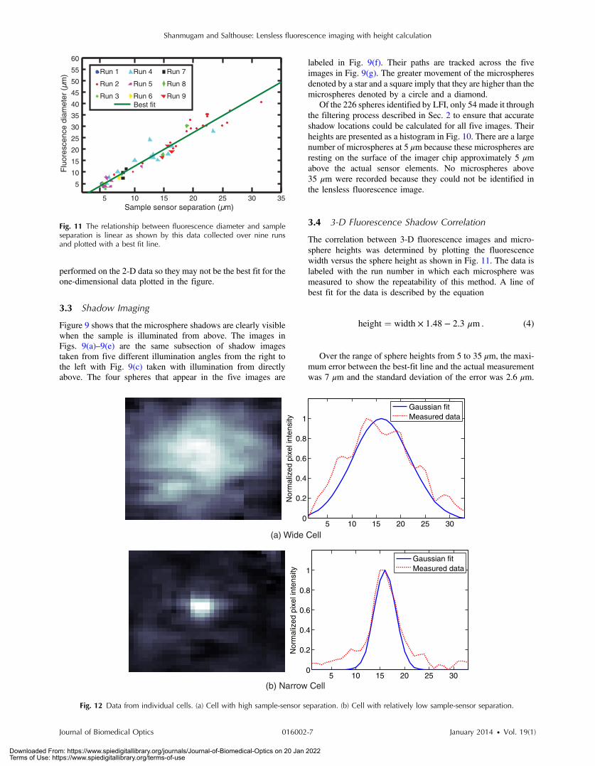
The correlation between 3-D fluorescence images and micro-sphere heights was determined by plotting the fluorescencewidth versus the sphere height as shown in Fig. 11. The data islabeled with the run number in which each microsphere wasmeasured to show the repeatability of this method. A line ofbest fit for the data is described by the equation

height ¼ width × 1.48 − 2.3 μm : (4)

Over the range of sphere heights from 5 to 35 μm, the maxi-mum error between the best-fit line and the actual measurementwas 7 μm and the standard deviation of the error was 2.6 μm.

5 10 15 20 25 30 35

5

10

15

20

25

30

35

40

45

50

55

60

Sample sensor separation (µm)

Flu

ores

cenc

e di

amet

er (

µm)

Run 1

Run 2

Run 3

Run 4

Run 5

Run 6

Run 7

Run 8

Run 9Best fit

Fig. 11 The relationship between fluorescence diameter and sampleseparation is linear as shown by this data collected over nine runsand plotted with a best fit line.

5 10 15 20 25 300

0.2

0.4

0.6

0.8

1

Nor

mal

ized

pix

el in

tens

ity


5 10 15 20 25 300

0.2

0.4

0.6

0.8

1

Nor

mal

ized

pix

el in

tens

ity


(a) Wide Cell

(b) Narrow Cell

Fig. 12 Data from individual cells. (a) Cell with high sample-sensor separation. (b) Cell with relatively low sample-sensor separation.




3.5 Lensless Fluorescence Imaging of FlowingSamples

Cells could not survive the procedure used to suspend micro-spheres in agarose, so LFI of cells was performed with thecells in liquid suspension. In the first experiment, detached cellsstained with quantum dots were mixed with fresh media andplaced on the imager and allowed to evaporate. The sample wasexcited with a UV source and images were captured as the waterevaporated. As shown in Fig. 12, despite the more complicatedgeometry of the cell compared to microspheres, the lenslessfluorescence image is still well modeled by a Gaussian curve.

To demonstrate that the technique works with a flowing sam-ple, the imager with the microfluidic device was employed. Thesample was pumped into the microfluidic channel and excitedwith a UV source. A video of the sample flowing through thechambers was captured. Figure 13 contains frames from the videodemonstrating movement of microspheres [Figs. 13(a)–13(c)]and cells [Figs. 13(d)–13(f)].

4 DiscussionFluorescence detection is an attractive technology for integrationin lab-on-a-chip systems because it offers high selectivity andsensitivity, but its use has been limited due to the high cost ofexisting techniques.21 LFI is well suited for integration becauseit only uses two components, an unfocused light source and anintegrated circuit. In this work, the light source was a low-pres-sure mercury bulb, but in future versions more compact lightemitting diodes will likely be used. In addition to performing im-aging, the integrated circuit can perform logical control opera-tions, image processing, and communication. This addedcomplexity is especially useful for digital microfluidic devices.22

The biggest challenge to LFI has been the need to tightlycontrol the spacing between the sample and the sensor. In prac-tice, this has limited the technique to applications where thesample is only measured in a thin layer directly on top of thesensor either due to the use of total internal reflection for

excitation16 or because the labeled cells are only found at thesurface.17,18

The work presented here demonstrates both the tradeoffbetween separation and LFI performance and a method formeasuring separation based on the measured fluorescenceimage. The data presented in this paper can be used to determinethe height of microfluidic channels for LFI in applications thatonly require fluorescent cell counting. For applications thatrequire 3-D cell tracking, the image processing techniques pre-sented here could be used. As the results show, the functionalityof this device can be extended to implement a flow cytometerwithout increasing the complexity of the imaging system.Delivering these results by employing only an imager and aUV source without the use of any optics makes the devicerobust, low cost, and easy to use in resource-limited areas.

5 ConclusionThis work has shown that the challenge of tightly controlling thesample-sensor separation for LFI can be relaxed by performingimage processing to calculate the height of fluorescently labeledcells. Initial evidence was presented in the form of simulationsfrom first principles. Based on the results of those simulations,an experiment was designed based on the fluorescently labeledspheres. A calibration method by fixing these spheres at preciselocations just microns above the imager surface was developed.The height of each sphere was then calculated using a simpletrigonometric technique based on shadow imaging. Then LFIwas performed on the sample. An image processing techniquewas developed for estimating the height of the sphere based ononly the fluorescence measurement. Finally, LFI was demon-strated in flowing cells in a microfluidic network.

Appendix: Derivation of Point IlluminationPatternA closed form solution for the illumination from a point sourcecan be calculated by considering a point light source at a dis-tance Z above an infinite plane. The illumination pattern will be

(c)(b)(a)

(f)(e)(d)

Fig. 13 Frames highlighting the movement of sample inside a lensless on-sensor microfluidic device (a)–(c) movement of microspheres (d)–(f) move-ment of quantum dot labeled RAW cells.




axially symmetric about a line perpendicular to the plane goingto the point light source. A unit sphere is placed around the pointlight source. Since the light source is omnidirectional, the lightflux will have a constant density throughout the unit sphere.

The illumination pattern on the plane can be determined byconstructing a right triangle where the hypotenuse is the linebetween the point in the plane and the light source, one legis in the plane, and the other leg is perpendicular to the plane.Rotating this right triangle around the symmetry line creates acone with a disk on the plane. The total illumination within thatdisk is proportional to the surface area of the unit sphereenclosed by the cone. This area can be calculated using sphericalcoordinates centered on the point light source

Areasphere ¼Z

2π

0

ZΘ1

0

sin θ∂θ∂ϕ;

Areasphere ¼ 2π

ZΘ1

0

sin θ∂θ;

Areasphere ¼ 2π½− cos θ�Θ1

0 ;

Areasphere ¼ 2π

�1 − cos

�arctan

�ZX

��;

Areasphere ¼ 2π

�1 −

ZffiffiffiffiffiffiffiffiffiffiffiffiffiffiffiffiffiZ2 þ X2

p�;

The illumination falling on the outside ring of the disk canthen be calculated by taking the ratio of the derivatives of growthof the area of the sphere and the area of the disk

∂Areasphere∂X

¼ 2π2XZ�12

ðZ2 þ X2Þ32 ¼

2πXZ

ðZ2 þ X2Þ32 ;

∂Areadisk∂X

¼ 2πX;

∂Areasphere∂Arearing

¼ Z

ðZ2 þ X2Þ32 :

AcknowledgmentsThis work was supported by the Dev and Linda GuptaEndowment and NSF Grant No. 1128558.

References1. J. Wolcott, A. Schwartz, and C. Goodman, “Laboratory medicine: a

national status report,” Prep. Centers Dis. Control Prev. (2008).

2. R. J. Buesa, “Current status of cytology laboratories in anatomicpathology departments,” Ann. Diagn. Pathol. 14(5), 347–354(2010).

3. I. Balachandran andM. Friedlander, “Cytology workforce study a reportof current practices and trends in New York State,” Am. J. Clin. Pathol.136(1), 108–118 (2011).

4. J. L. Weaver and M. Stetler-Stevenson, “Flow cytometry in the biomedi-cal arena,” Medical Biomethods Handbook, pp. 531–553, Springer-Verlag, New York (2005).

5. M. Alunni-Fabbroni and M. T. Sandri, “Circulating tumour cells inclinical practice: methods of detection and possible characterization,”Methods San Diego Calif. 50, 289–297 (2010).

6. D. A. Ateya et al., “The good, the bad, and the tiny: a review ofmicroflow cytometry,” Anal. Bioanal. Chem. 391(5), 1485–1498(2008).

7. S. C. Lin et al., “Channel layer, single sheath-flow inlet microfluidicflow cytometer with three-dimensional hydrodynamic focusing,” LabChip 12(17), 3135–3141 (2012).

8. S. W. Kettlitz et al., “Planar microfluidic chip employing a light emittingdiode and a PIN-photodiode for portable flow cytometers,” Lab Chip12, 197–203 (2011).

9. Y. J. Fan, H. J. Sheen, and P. Y. Chiou, “High throughput and parallelflow cytometer with solid immersion microball lens array,” in 2012IEEE 25th Int. Conf. Micro Electro Mech. Syst. Mems, Paris,pp. 1041–1044 (2012).

10. A. Ozcan and U. Demirci, “Ultra wide-field lens-free monitoring ofcells on-chip,” Lab Chip 8(1), 98–106 (2007).

11. O. Mudanyali et al., “Lensless on-chip imaging of cells provides anew tool for high-throughput cell-biology and medical diagnostics,”J. Visualized Exp. 34, e1650 (2009).

12. T. Su et al., “Multi-angle lensless digital holography for depth resolvedimaging on a chip,” Opt. Express 18(9), 9690–9711 (2010).

13. J. Weidling et al., “Lens-free computational imaging of capillarymorphogenesis within three-dimensional substrates,” J. Biomed. Opt.17(12), 126018 (2012).

14. T. Su, L. Xue, and A. Ozcan, “High-throughput lensfree 3D tracking ofhuman sperms reveals rare statistics of helical trajectories,” Proc. Natl.Acad. Sci. U. S. A. 109(40), 16018–16022 (2012).

15. T. Su et al., “Sperm trajectories from chiral ribbons,” Sci. Rep. 3, 1664(2013).

16. A. F. Coskun et al., “Lensfree fluorescent on-chip imaging of transgenicCaenorhabditis elegans over an ultra-wide field-of-view,” PLoS One 6,e15955 (2011).

17. E. P. Dupont et al., “Fluorescent magnetic bead and cell differentiation/counting using a CMOS SPAD matrix,” Sens. Actuators B 174, 609–615 (2012).

18. W. Li et al., “On-chip integrated lensless fluorescence microscopy/spec-troscopy module for cell-based sensors,” Proc. SPIE 7894, 78940Q(2011).

19. A. F. Coskun et al., “Lensfree wide-field fluorescent imaging on a chipusing compressive decoding of sparse objects,” Opt. Express 18(10),10510–10523 (2010).

20. H. Han, M. Kriman, and M. Boomgarden, “Wafer level camera tech-nology—from wafer level packaging to wafer level integration,” in 201011th Int. Conf. Electron. Packag. Technol. High Density Packag.(ICEPT-HDP), Xi'an, pp. 121–124 (2010).

21. J. Wu and M. Gu, “Microfluidic sensing: state of the art fabrication anddetection techniques,” J. Biomed. Opt. 16(8), 080901 (2011).

22. J. Nichols et al., “On-chip digital microfluidic architectures forenhanced actuation and sensing,” J. Biomed. Opt. 17(16), 067005(2012).




http://dx.doi.org/10.1016/j.anndiagpath.2010.07.005

http://dx.doi.org/10.1309/AJCPUDFRALJY32XM

http://dx.doi.org/10.1007/s00216-007-1827-5

http://dx.doi.org/10.1039/c1lc20672a

http://dx.doi.org/10.1039/b713695a

http://dx.doi.org/10.3791/1650

http://dx.doi.org/10.1364/OE.18.009690


http://dx.doi.org/10.1073/pnas.1212506109

http://dx.doi.org/10.1073/pnas.1212506109

http://dx.doi.org/10.1038/srep01664

http://dx.doi.org/10.1371/journal.pone.0015955

http://dx.doi.org/10.1016/j.snb.2012.06.049

http://dx.doi.org/10.1117/12.875417

http://dx.doi.org/10.1364/OE.18.010510

http://dx.doi.org/10.1117/1.3607430


lensless fluorescence imaging with height calculation

Documents