lexical analysis/scanningcse.iitkgp.ac.in/~goutam/iiitkalyani/compiler/lect/lect2.pdfthe states of...

Compiler Design IIIT Kalyani, WB 1✬

✫

✩

✪

Lexical Analysis/Scanning

Lect 2 Goutam Biswas


✫

✩

✪

Input and Output

The input is a stream of characters (ASCII

codes) of the source program.

The output is a stream of tokens or symbolscorresponding to different syntactic categories.The output also contains attributes of tokens.Examples of tokens are different keywords,identifiers, constants, operators, delimiters etc.



✫

✩

✪

Note

The scanner removes the comments, white

spaces, evaluates the constants, keeps track of

the line numbers etc.

This stage performs the main I/O and reduces

the complexity of the syntax analyzer.

The syntax analyzer invokes the scannerwhenever it requires a token.



✫

✩

✪

Token

A token is an identifier (name/code)corresponding to a syntactic category of thelanguage grammar. In other word it is symbol(terminal) of the alphabet of the grammar.Often we use an integer code for this.



✫

✩

✪

Pattern

A pattern is a description (formal or informal)of the set of objects corresponding to a terminal(token) symbol of the grammar. Examples arethe set of identifier in C language, set of integerconstants etc.



✫

✩

✪

Lexeme and Attribute

A lexeme is the actual string of characters that

matches with a pattern and generates a token.

An attribute of a token is a value that thescanner extracts from the corresponding lexemeand supplies to the syntax analyzer. Typicalexamples are values of constants, actual stringof characters of identifiers etc.



✫

✩

✪

Specification of Token

The set of strings corresponding to a token(terminals) of a programming language is oftena regular set and is specified by a regularexpression.



✫

✩

✪

Scanner from the Specification

The collection of tokens of a programminglanguage can be specified by a set of regularexpressions. A scanner or lexical analyzer forthe language uses a DFA (recognizer of regularlanguages) in its core. Different final states ofthe DFA identifies different tokens. Synthesis ofthis DFA from the set of regular expressionscan be automated.



✫

✩

✪

Regular Expression

1. ε, ∅ and all a ∈ Σ are regular expressions.

2. If r and s are regular expressions, then so

are (r|s), (rs), (r∗) and (r). Nothing else is a

regular expression.

We can reduce the use of parenthesis byintroducing precedence and associativity rules.Binary operators are left associative and theprecedence rule is ∗ > concat > |.



✫

✩

✪

IEEE POSIX Regular Expression

An enlarged set of operators (defined) for the

regular expressions are introduced in different

software e.g. awk, grep, lex etc.a.

• \x is the character itself (a few exceptions

are \n, \t, \r etc.).

• . is any character other than ‘\n’.

• [xyz] is x | y | z.aConsult the manual pages of lex/flex and Wikipedia for the details of IEEE

POSIX standard of regular expressions.



✫

✩

✪

IEEE POSIX Regular Expression

• [abg-pT-Y] any character a, b,g, · · · , p,

T, · · · , Y.

• [^G-Q] not any one of G, H, · · · , P, Q.

• r+ one or more r’s.

• r? one or zero r’s.

• r{2,} two or more r’s etc.



✫

✩

✪

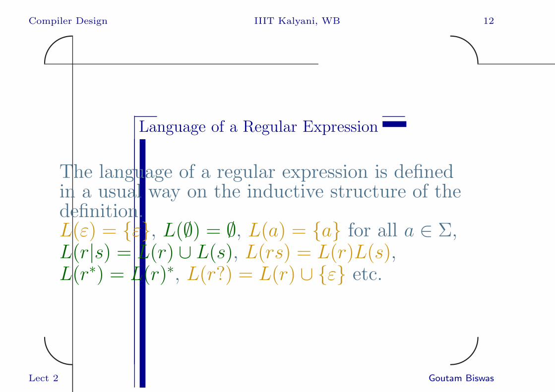
Language of a Regular Expression

The language of a regular expression is definedin a usual way on the inductive structure of thedefinition.L(ε) = {ε}, L(∅) = ∅, L(a) = {a} for all a ∈ Σ,L(r|s) = L(r) ∪ L(s), L(rs) = L(r)L(s),L(r∗) = L(r)∗, L(r?) = L(r) ∪ {ε} etc.



✫

✩

✪

C Identifier

The regular expression for the C identifier is[ a-zA-Z][ a-zA-Z0-9]*The first character is an underscore or anEnglish alphabet. From the second character ona decimal digit can also be used.



✫

✩

✪

Regular Definition

We can give name to a regular expression forthe convenience of use. A name of a regularexpression can be used in the following regularexpressions as a meta symbol.



✫

✩

✪

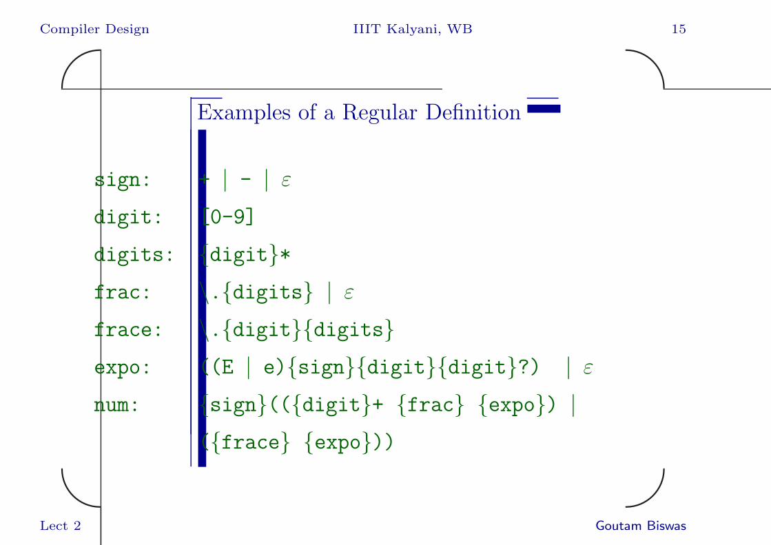
Examples of a Regular Definition

sign: + | - | ε

digit: [0-9]

digits: {digit}*

frac: \.{digits} | ε

frace: \.{digit}{digits}

expo: ((E | e){sign}{digit}{digit}?) | ε

num: {sign}(({digit}+ {frac} {expo}) |

({frace} {expo}))



✫

✩

✪

RE to NFA: Thompson’s Construction

• For each a ∈ Σ we can construct a 2-state

NFA to recognize ‘a’.

• We can combine these base NFAs using

ε-transitions to build bigger NFAs.

• All these NAFs have one initial and one final

state.



✫

✩

✪

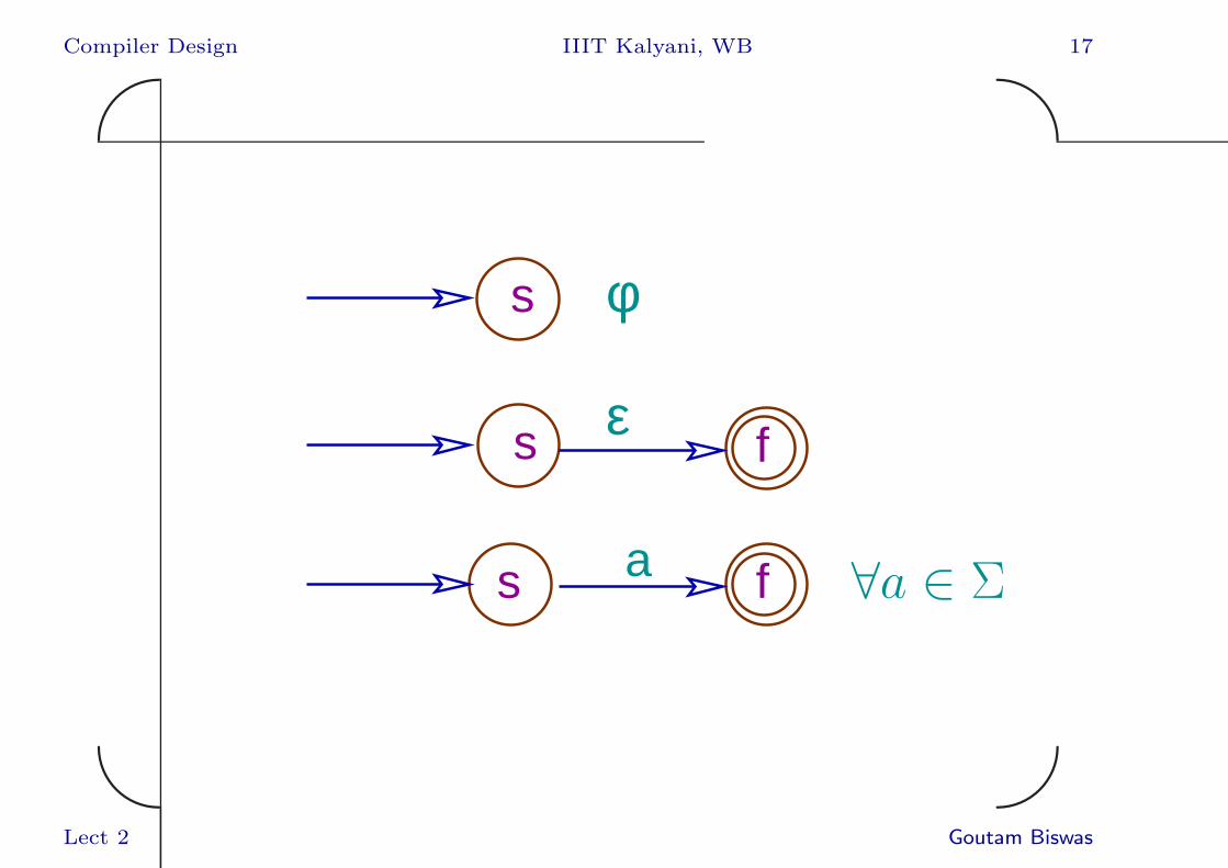
φ

ε

a

s

f

f

s

s

∀a ∈ Σ



✫

✩

✪

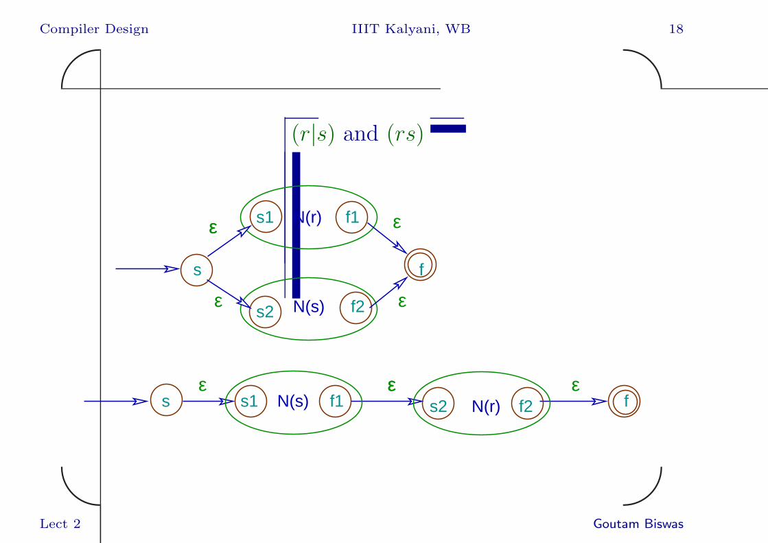
(r|s) and (rs)

s1

s2

f1

f2

s f

s1 s2f1 f2s f

εε

ε

ε

ε

εεε ε

N(r)

N(s)

N(s) N(r)



✫

✩

✪

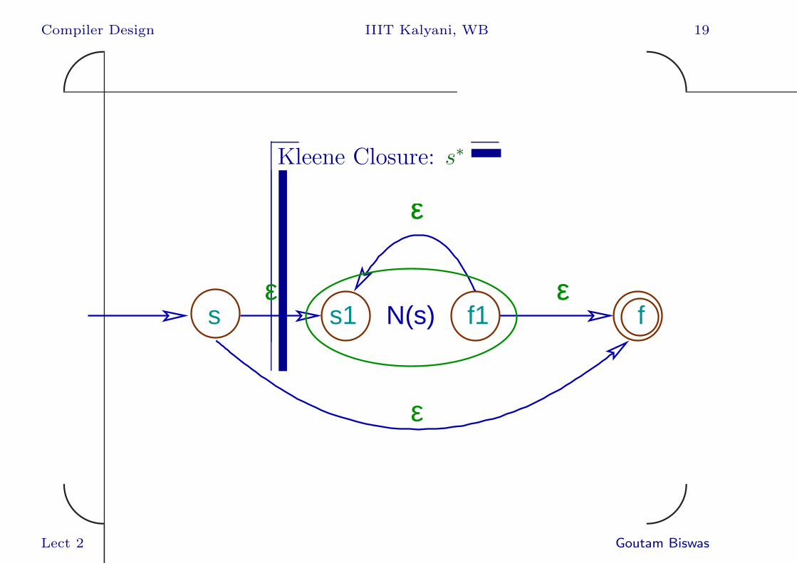
Kleene Closure: s∗

s1 f1sεεε

f

εεε

ε

N(s)



✫

✩

✪

Properties of Thompson’s Construction

• |Q| ≤ 2length(r), where Q is the number of

states of the NFA and length(r) is the

number of alphabet and operator symbols in

r.

• Only one initial and one final state. No

incoming edge to the initial state and no

outgoing edge from the final state.



✫

✩

✪

Properties of Thompson’s Construction

• At most one incoming and one outgoing

transition on a symbol of the alphabet. At

most two incoming and two outgoing

ε−transitions.



✫

✩

✪

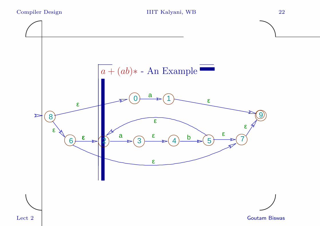
a+ (ab)∗ - An Example

a bεε ε

ε

εε

ε

aε

ε

ε

ε

0 1

2 3 4 56 7

8 9



✫

✩

✪

Context-Free Grammar of RE

The set of regular expression can be specified

by a context-free grammar.

E → ∅ | ε | σ, ∀σ ∈ Σ

→ E.E | E + E | E ∗ | (E)

We have put a ‘.’ for concatenation to make itan operator grammar and have replaced ‘|’ by‘+’ for claritya.

aThis ambiguous grammar can be used with proper precedence and associa-

tivity rules.



✫

✩

✪

Syntax Directed Thompson’s Construction

Rules of Thompson’s construction can beassociated with the non-terminals of theproduction rules of the grammar. This isknown as an attribute grammar. We assumethe following data structures.



✫

✩

✪

Syntax Directed Thompson’s Construction

• Global state counter S initialized to 0, and

the state transition table: T[][].

• With every occurrence of the non-terminal E

we associate two attributes E.ini and E.fin

to store the initial and the final states of the

NFA, corresponding to the regular expression

generated by this occurrence of E.



✫

✩

✪

Some of the Rules: Basis

E → ε: {T[S][ε] = S+1; E.ini = S;

S = S+1; E.fin = S; S = S+1;}

E → a: {T[S][a] = S+1; E.ini = S;

S = S+1; E.fin = S; S = S+1;}

The second rule depends on the symbol of thealphabet



✫

✩

✪

Concatenation Rules

E → E1.E2: {E.ini = S; S = S+1;

E.fin = S+1; S = S+1;

T[E.ini][ε]=E1.ini;

T[E1.fin][ε]=E2.ini;

T[E2.fin][ε]=E.fin;}

Similarly other rules can be derived.



✫

✩

✪

The Final NFA

The states of the final NFA are{0, 1, · · · , S − 1}. The initial state is in E.iniand the final state is in E.fin. The statetransitions are in T[][].



✫

✩

✪

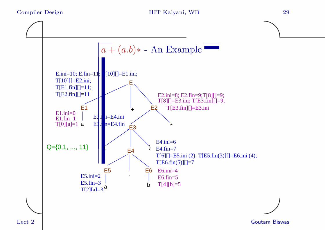
a+ (a.b)∗ - An Example

+

( )

*a

a b

.

T[10][]=E2.ini;T[E1.fin][]=11;T[E2.fin][]=11

E1.ini=0E1.fin=1T[0][a]=1

E3.ini=E4.iniE3.fin=E4.fin

E5.ini=2E5.fin=3T[2][a]=3

E6.ini=4E6.fin=5T[4][b]=5

E4.ini=6E4.fin=7T[6][]=E5.ini (2); T[E5.fin(3)][]=E6.ini (4);T[E6.fin(5)][]=7

T[8][]=E3.ini; T[E3.fin][]=9;E2.ini=8; E2.fin=9;T[8][]=9;

E

E1 E2 T[E3.fin][]=E3.ini

E3

E4

E5

E.ini=10; E.fin=11; T[10][]=E1.ini;

E6

Q={0,1, ..., 11}



✫

✩

✪

Construction of DFA from NFA

Let the constructed ε-NFA be(N,Σ, δn, n0, {nF}). By taking ε-closure ofstates and doing the subset construction we canget an equivalent DFA (Q,Σ, δd, q0, QF ).



✫

✩

✪

Algorithm: Subset Construction

q0 = ε-closure({n0})

Q = L = {q0}

while(L 6= ∅)

q = removeElm(L)

for all σ ∈ Σ

t = ε-closure(δn(q, σ))

T [q][σ] = t

if t 6∈ Q

Q = Q ∪ {t}

L = L ∪ {t}



✫

✩

✪

ε-closure(T )

for all n ∈ T push(S, n) // S is stack

εT = T

while(notEmpty(S))

n = pop(S)

for all n′ ∈ δ(n, ε)

if n′ 6∈ εT

εT = εT ∪ {n′}

push(S, n′)



✫

✩

✪

Final State of the DFA

The set of final states of the equivalent DFA isQF = {q ∈ Q : nF ∈ q}. It is to be noted thatdifferent final states will recognize differenttokens. It is also possible that one final stateidentifies more than one tokens.



✫

✩

✪

Time Complexity of Subset Construction

The size of Q is O(2|N |) and so the timecomplexity is also O(2|N |), where N is the set ofstates of the NFA. But this is one timeconstruction.



✫

✩

✪

a+ (ab)∗ - NFA to DFA

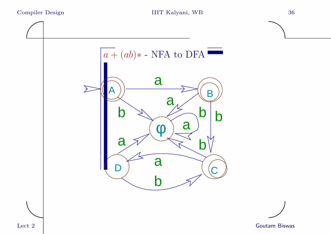
The state transition table of the DFA is

Initial Final State

State a b

A : {0, 2, 6, 7, 8, 9} {1, 3, 4, 9} ∅

B : {1, 3, 4, 9} ∅ {2, 5, 7, 9}

C : {2, 5, 7, 9} {3, 4} ∅

D : {3, 4} ∅ {2, 5, 7, 9}

∅ ∅ ∅



✫

✩

✪

a+ (ab)∗ - NFA to DFA

aa

aa

a

b bb

b

b

φ

D

A B

C



✫

✩

✪

Note

• We may drop the transitions to ∅ for

designing a scanner. This makes the DFA

incompletely specified.

• Absence of a transition from a final state

identifies a token.

• But in a scanner absence of a transition from

a non-final state may be due to crossing past

a token.



✫

✩

✪

DFA State Minimization

• The constructed DFA may have set of

equivalent statesa and can be minimized.

• The time complexity of a scanner with lesser

number of states is not different from one

with smaller number of states.

• Their code sizes may be different.

aLet M = (Q,Σ, δ, s, F ) be a DFA. Two states p, q ∈ Q are said to be equiv-

alent if there is no x ∈ Σ∗ so that δ(p, x) 6= δ(q, x).



✫

✩

✪

DFA State Minimization

• Minimization starts with two non-equivalent

partitions of Q: F and Q \ F .

• If p, q belongs to the same initial partition P

of states, but there is some σ ∈ Σ so that

δ(p, σ) ∈ P1 and δ(q, σ) ∈ P2, where P1 and

P2 are two distinct partitions, then p, q

cannot remain in the same partition i.e. they

are not equivalent.



✫

✩

✪

DFA to Scanner

• Given a regular expression r we can

construct a recognizer of L(r).

• For every token class or syntactic category of

a language we have a regular expression.

• Let {r1, r2, · · · , rk} be the total collection of

regular expressions of a language. Then

r = r1|r2| · · · |rk represents objects of all

syntactic categories.



✫

✩

✪

DFA to Scanner

• Given the set of NFAs of r1, r2, · · · , rk we

construct the NFA for r = r1|r2| · · · |rk by

introducing a new start state and adding

ε-transitions from this state to the initial

states of the component NFAs.

• But we keep different final states as they are

to identify different tokens.



✫

✩

✪

Final Composite NFA

sr1 fr1

sr2 fr2

srk frk

ε

ε

ε

s

N(r1)

N(r2)

N(rk)



✫

✩

✪

DFA to Scanner

The DFA corresponding to r can beconstructed from the composite NFA. It can beimplemented as a C program that will be usedas a scanner of the language. But the followingpoints are to be noted.



✫

✩

✪

Note

• A lexically correct program is not a single

word but a stream of words.

• The dynamics of acceptance of a word in a

scanner is slightly different from a simple

DFA.

• Words of different syntactic categories are

often not separated by delimiters.



✫

✩

✪

Note

• Word of one syntactic category may be a

prefix of a word of another category.

• We need to address the following questions.

– when does the scanner report an

acceptance?

– what does it do if the word (lexeme)

matches with more than one regular

expressions?



✫

✩

✪

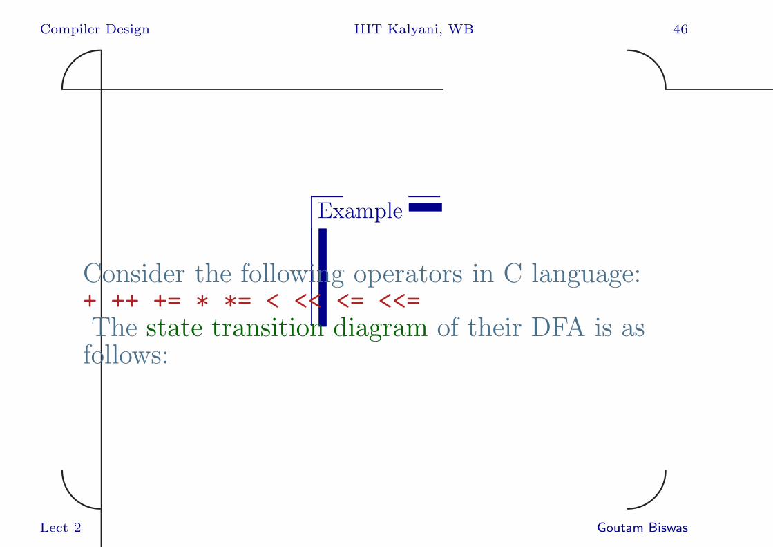
Example

Consider the following operators in C language:+ ++ += * *= < << <= <<=The state transition diagram of their DFA is asfollows:



✫

✩

✪

2

3

4

5

6

7

8

+

=

* =

<< =

=

1+

9

a

b

c d

nts

nts

nts

nts

nts

nts

nts

nts

nts

nts: no transition specified



✫

✩

✪

Note

• Both state a and 1 are final. The token for

++ can be generated at state 1 as it is not

prefix to any other pattern.

• But it cannot be done at state a without a

look-ahead. If the next symbol is other than

+ or =, then the token for + can be

generated.



✫

✩

✪

Note

• The amount of look-ahead may be more

than one character.

• The look-ahead symbols are put back in the

input stream before starting the matching

for the next pattern (from the start state).



✫

✩

✪

A Classic Example

• Here is a situations where there are more

than one look-ahead.

Fortran:DO 10 I = 1, 10 and DO 10 I = 1.10The first one is a do-loop and the second one isan assignment DO10I=1.10. Fortran ignoresblanks.PL/I:IF ELSE THEN THEN = ELSE; ELSE ELSE = THENIF THEN are not reserved as keyword.



✫

✩

✪

Maximum Word Length Matching

• The scanner will go on reading input as long

as there is a transition on it from the current

state.

• Let there be no transitions from the current

state q on the next input σ (the machine is

incompletely specified).

• The state q may or may not be a final state.



✫

✩

✪

q is Final

• If the final state q corresponds to only one

regular expression ri, the scanner returns the

corresponding tokena.

• But if it matches with more than one regular

expressions then the conflict is resolved by

specifying priority of expressions e.g. a

keyword over an identifier.aIt is necessary to identify the final state of the DFA with regular expressions.

It is determined by the final states of the NFA present in the final state of the

DFA.



✫

✩

✪

q is not Final

• It is possible that while consuming symbols

the scanner has crossed one or more final

states. In a maximal length scanner, the

token corresponding to the last final state is

returned.

• So it is necessary to keep track of the

sequence of states crossed before a final state

is reacheda.aA stack may be used for this purpose.



✫

✩

✪

Components of a Scanner

1. The transition table of the DFA or NFAa.

2. Set of actions corresponding to terminal and

final states.

3. Other essential functions.aThe table may be kept explicitly or implicitly (in the code).



✫

✩

✪

Maximum Prefix on NFA

• Read input and keep track of the sequence of

the set of states. Stop when no more

transition is possible (maximum prefix).

• Trace the set of states backward and stop

when a set of states with one or more final

states is reached.



✫

✩

✪

Maximum Prefix on NFA

• Push back the look-ahead symbols in the

input buffer and emit appropriate token

along with attribute value(s).

• The set of states may have more than one

final states corresponding to different

patterns. Action is taken corresponding to a

pattern with highest priority.



✫

✩

✪

From DFA to Code

Most often a DFA is used to implement a

scanner. There are three possible

implementations.

• Table driven,

• Direct coded,

• Hand coded.

We shall discuss about the table driven one indetail.



✫

✩

✪

Table Driven Scanner

There is a driver code and a set of tables. The

driver code essentially has three componentss:

• Initialization,

• Main scanner loop,

• Roll-back loop,

• Token or error return.



✫

✩

✪

Initialization

cs ← q0 # current state is start state

lexme ← “ ” # null string

push(S, $) # push end of stack marker



✫

✩

✪

Scanner Loop

while cs 6= φ # current state is not sink state

lexme ← lexme + (c = getchar()) # read next symbol

if cs ∈ QF then clear(S) # clear stack if cs is final

push(S, cs) # push current state

sym ← trans[c] # translate char to DFA symbol

cs ← δ(cs, sym) # current state is next state



✫

✩

✪

Roll Back Loop

while cs 6∈ QF and notEmpty(S)

# current state is not a final state and stack is not empty

cs ← pop(S) # pop new state from stack

unget() last symbol of lexme.



✫

✩

✪

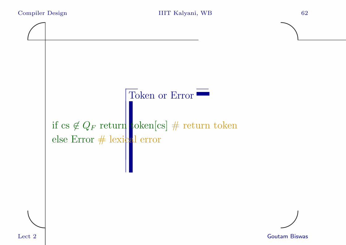
Token or Error

if cs 6∈ QF return token[cs] # return token

else Error # lexical error



✫

✩

✪

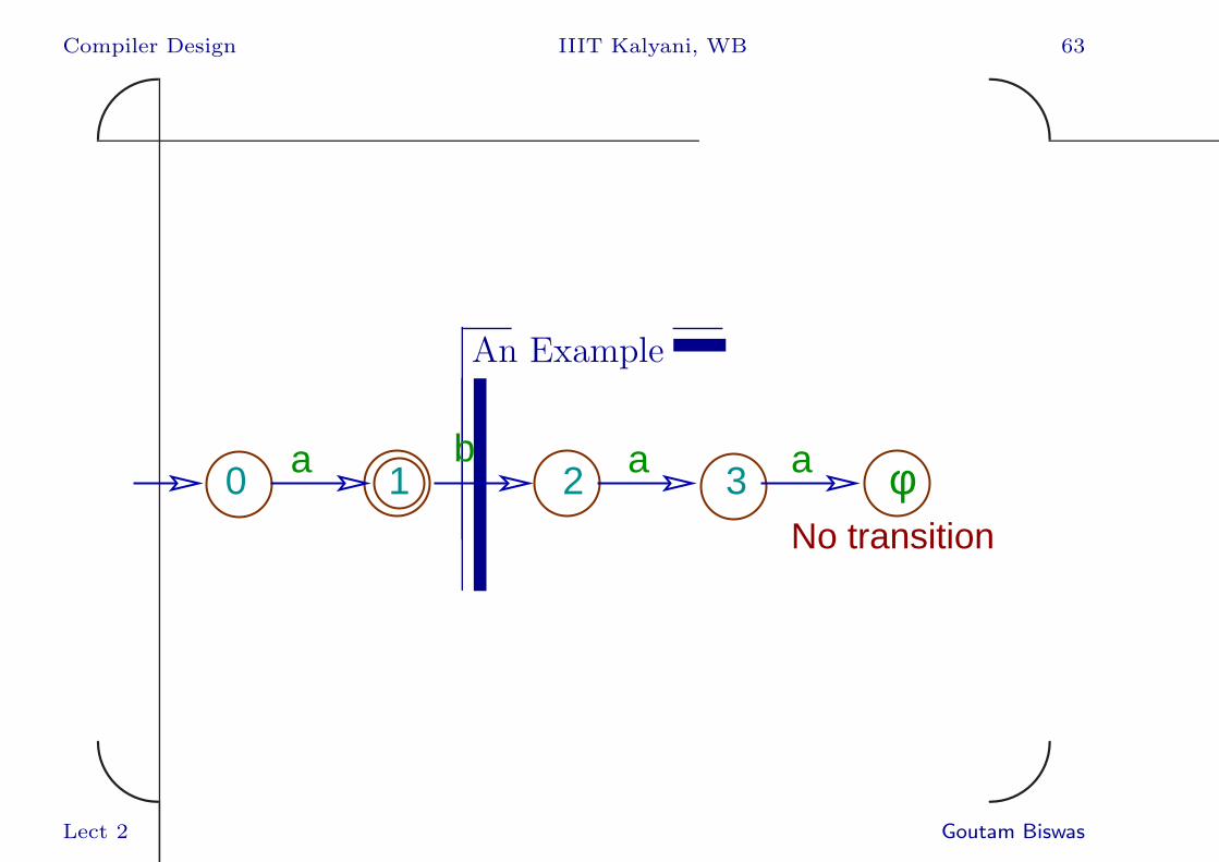
An Example

φ0 1 2 3a b a a

No transition



✫

✩

✪

Example

• After initialization: cs = 0, stack: empty [$],

lexeme = null.

• After the scanner loop: cs = φ, stack:

[$ 1 2 3], lexeme = ”abaa”.

• After the roll back loop: cs = 1, stack:

empty [$], lexeme = ”a”

• Token for state 1 is generated.



✫

✩

✪

Tables

• translate[] converts a character to a DFA

symbol (reduces the size of the alphabet).

• delta[] is the state transition table.

• token[] have token values corresponding to

final states.



✫

✩

✪

Quadratic Roll-Back

At times roll-back may be costly - consider thelanguage ab|(ab)∗c and the input ababababab$.There will be roll-back of 8 + 6 + 4 + 2 = 20characters.



✫

✩

✪

Direct Coded Scanner

• Each state is implemented as a fragment of

code.

• It eliminates memory reference for transition

table access.



✫

✩

✪

Code Corresponding to a State

• Code is labelled by the state name.

• Read a character and append it to lexeme.

• Update the roll-back stack.

• Go to next appropriate state - a valid

transition, roll-back and token return state

etc.



✫

✩

✪

Reading Characters: Input Buffer

• A scanner or lexical analyzer reads the input

character by character. The process will be

very inefficienta if the scanner sends request

to the OS to read each character.

• So the scanner reads a block of characters in

a local buffer and consumes it one character

at a time.aSystem call is costly even if the data is available most of the time in the

buffer cache.



✫

✩

✪

Input Buffer

• A buffer at its end may contain the initial

portion of a lexeme. It creates problem in

refilling the buffer. So a 2-buffer scheme is

used. The buffers are filled alternately.

• A sentinel-character is placed at the

end-of-buffer to avoid two comparisons -

character and end-of-buffer.



✫

✩

✪

Direct Construction of DFA from a Regular Expression

A deterministic finite automaton can beconstructed directly from the given regularexpression.



✫

✩

✪

Definition: Important States

• All initial states of the NFA are important.

• Any other state p of the NFA is also

important if p has an out-transition on some

σ ∈ Σ.

• Let the NFA be (N,Σ, δn, n0, {nF}).



✫

✩

✪

Important States

• During the construction of DFA

(Q,Σ, δd, q0, QF ) from the NFA, we compute

the next state of the DFA as

ε-closure(δn(q, σ)), where q ⊆ N (q ∈ Q) and

σ ∈ Σ.

• In this computation only the important

states of the NFA belonging to q and their

ε-closures are useful.



✫

✩

✪

Important States

• Given a regular expression r the important

statesa of the NFA are determined by the

positions of symbols in the regular

expression.

• In our example, a+ (ab)∗ the important

states are 8, 0, 2, 4.

aOther than the initial state of the NFA.



✫

✩

✪

a+ (ab)∗ - An Example

a bεε ε

ε

εε

ε

aε

ε

ε

ε

0 1

2 3 4 56 7

8 9



✫

✩

✪

End Marker and Final State

We introduce a special end marker # 6∈ Σ tothe regular expression, r → (r)#. This makesthe final state(s) of the original NFA important.It also helps to detect the final state(s) (a statethat has transition on #).



✫

✩

✪

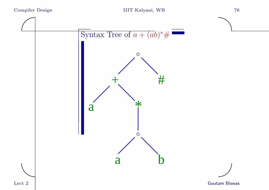
Syntax Tree of a Regular Expression

A regular expression can be represented by asyntax tree where each leaf node corresponds toa symbol of the alphabet, a ∈ Σ, or ε. Eachinternal node corresponds to an operatorsymbol.



✫

✩

✪

Syntax Tree of a+ (ab)∗#

#+

*a

a b



✫

✩

✪

Labelling the Leaf Nodes

• We associate a positive integer p with each

leaf node of a ∈ Σ (not of ε). The positive

integer p is called the position of the symbol

of the leaf node.

• Following are a few definitions where n is a

node and p is a position.



✫

✩

✪

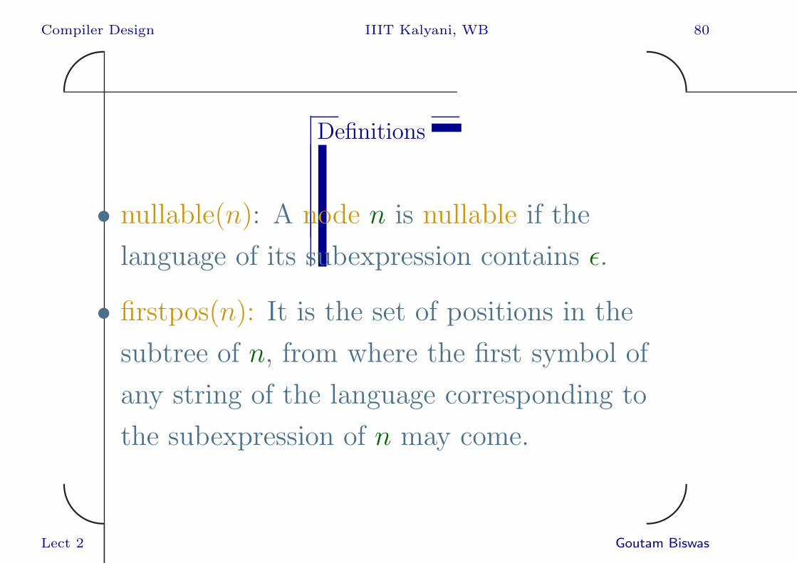
Definitions

• nullable(n): A node n is nullable if the

language of its subexpression contains ǫ.

• firstpos(n): It is the set of positions in the

subtree of n, from where the first symbol of

any string of the language corresponding to

the subexpression of n may come.



✫

✩

✪

Definitions

• lastpos(n): it is similar to the firstpos(n)

except that these are the positions of the

last symbols.

• followpos(p): It is the set positions in the

syntax tree from where a symbol may come

after the symbol of the position p in a string

of L((r)#).



✫

✩

✪

Computation of nullable(n)

n is a

• leaf node with label ε: true.

• leaf node with label a ∈ Σ: false.

• internal node of the form n1 + n2:

nullable(n1) ∨ nullable(n2).

• internal node of the form n1 ◦ n2:

nullable(n1) ∧ nullable(n2).

• internal node of the form n∗1: true.



✫

✩

✪

Computation of firstpos(n)

n is a

• leaf node with label ε: ∅.

• leaf node with label a ∈ Σ: {a}.

• internal node of the form n1 + n2: firstpos(n1) ∪

firstpos(n2).

• internal node of the form n1 ◦ n2: if nullable(n1), then

firstpos(n1) ∪ firstpos(n2), else firstpos(n1).

• internal node of the form n∗1: firstpos(n1).



✫

✩

✪

Computation of lastpos(n)

n is a

• leaf node with label ε: ∅.

• leaf node with label a ∈ Σ: {a}.

• internal node of the form n1 + n2: lastpos(n1) ∪

lastpos(n2).

• internal node of the form n1 ◦ n2: if nullable(n2), then

lastpos(n1) ∪ lastpos(n2), else lastpos(n2).

• internal node of the form n∗1: lastpos(n2).



✫

✩

✪

Example

In our example there are two nullable nodes,the ‘+’ and the ‘∗’ nodes. We decorate thesyntax tree with firstpos() and lastpos() data.



✫

✩

✪

#+

*a

a b

1

2 3

4

({3}, {3})

({1}, {1})

({2}, {2})

({2}, {3})

({2}, {3})

({4}, {4})({1, 2}, {1, 3})

({1, 2, 4}, {4})



✫

✩

✪

Computation of followpos(p)

Given a regular expression r, a symbol of a

particular position can be followed by a symbol

of another position in a string of L(r) in two

different ways.

• If n is a concatenation node n1 ◦ n2 of the

syntax tree, then for each position p in

lastpos(n1), each position q of firstpos(n2) is

in followpos(p).



✫

✩

✪

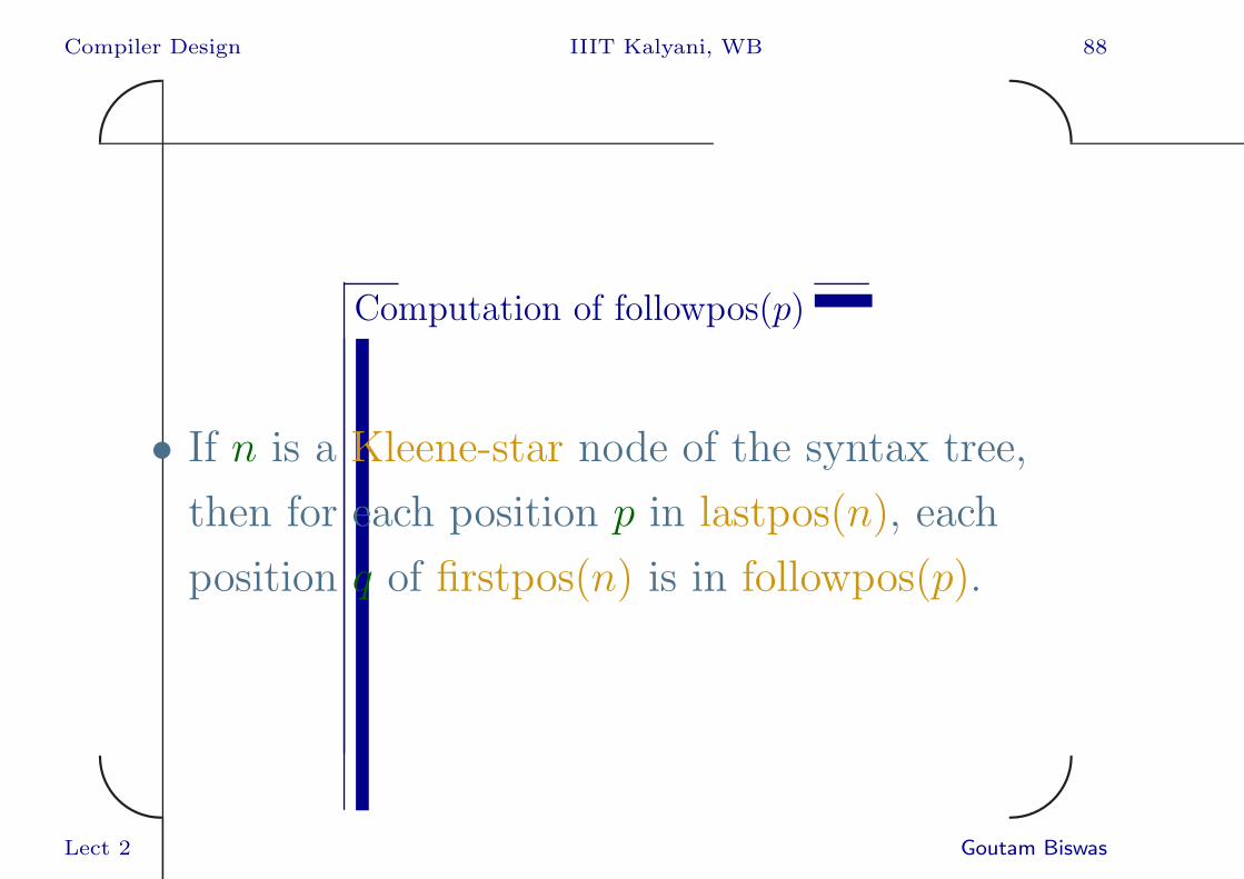
Computation of followpos(p)

• If n is a Kleene-star node of the syntax tree,

then for each position p in lastpos(n), each

position q of firstpos(n) is in followpos(p).



✫

✩

✪

Example

In our example,

• from the concatenation node we get that

3 ∈ followpos(2), 4 ∈ followpos(1) and

followpos(3).

• from the Kleene-star node we get

2 ∈ followpos(3).



✫

✩

✪

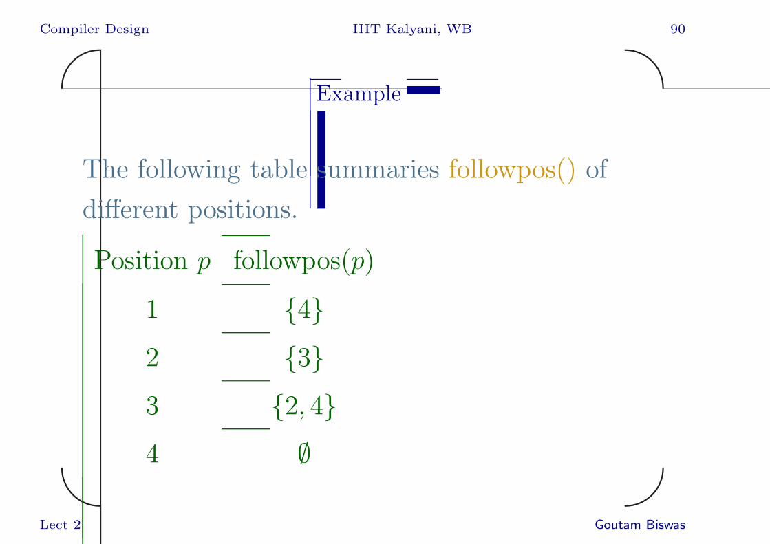
Example

The following table summaries followpos() of

different positions.

Position p followpos(p)

1 {4}

2 {3}

3 {2, 4}

4 ∅



✫

✩

✪

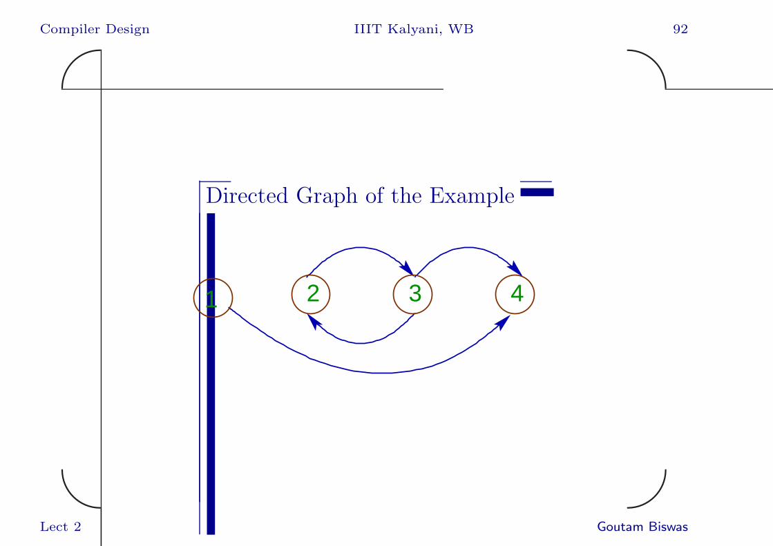
Directed Graph of followpos()

• Each position p is represented by a node.

• There is a directed edge from a position p to

a position q, if q ∈ followpos(p).



✫

✩

✪

Directed Graph of the Example

1 2 3 4



✫

✩

✪

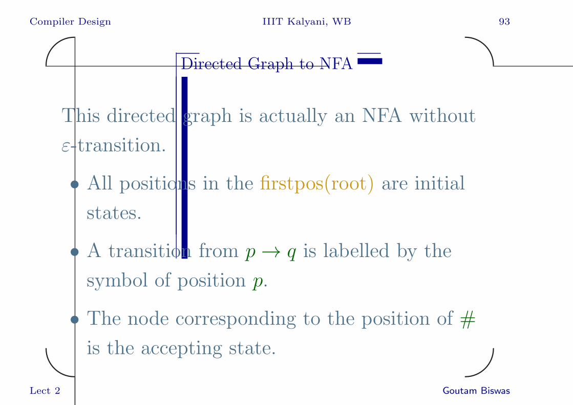
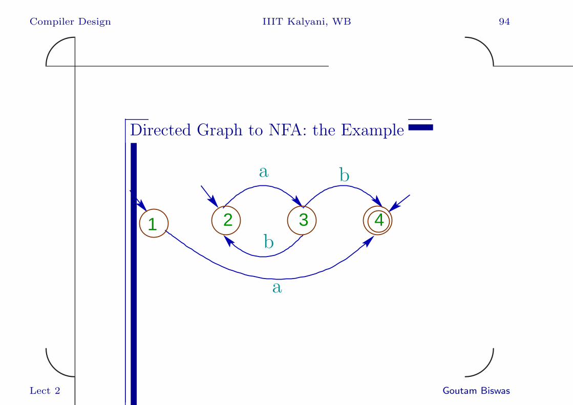
Directed Graph to NFA

This directed graph is actually an NFA without

ε-transition.

• All positions in the firstpos(root) are initial

states.

• A transition from p→ q is labelled by the

symbol of position p.

• The node corresponding to the position of #

is the accepting state.



✫

✩

✪

Directed Graph to NFA: the Example

1 2 3 4

a

a

b

b



✫

✩

✪

DFA from Regular Expression - Direct Construction

Input: A regular expression r over Σ

Output: A DFA M = (Q,Σ, s, F, δ).

Algorithm:

1. Construct a syntax tree T corresponding to

the augmented regular expression (r)#,

where # 6∈ Σ.



✫

✩

✪

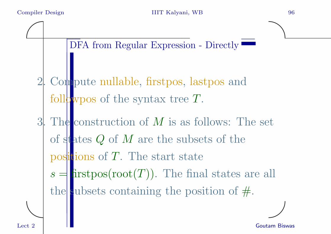
DFA from Regular Expression - Directly

2. Compute nullable, firstpos, lastpos and

followpos of the syntax tree T .

3. The construction of M is as follows: The set

of states Q of M are the subsets of the

positions of T . The start state

s = firstpos(root(T )). The final states are all

the subsets containing the position of #.



✫

✩

✪

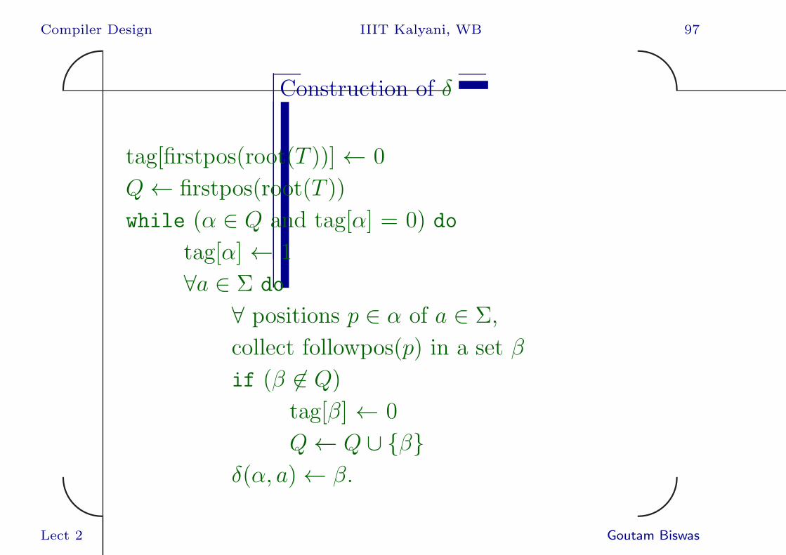
Construction of δ

tag[firstpos(root(T ))] ← 0

Q← firstpos(root(T ))

while (α ∈ Q and tag[α] = 0) do

tag[α] ← 1

∀a ∈ Σ do

∀ positions p ∈ α of a ∈ Σ,

collect followpos(p) in a set β

if (β 6∈ Q)

tag[β] ← 0

Q← Q ∪ {β}

δ(α, a)← β.



✫

✩

✪

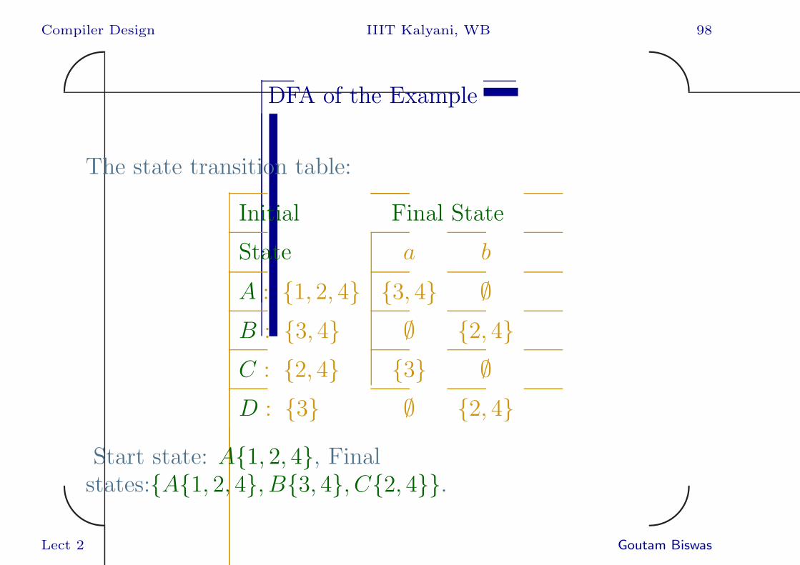
DFA of the Example

The state transition table:

Initial Final State

State a b

A : {1, 2, 4} {3, 4} ∅

B : {3, 4} ∅ {2, 4}

C : {2, 4} {3} ∅

D : {3} ∅ {2, 4}

Start state: A{1, 2, 4}, Finalstates:{A{1, 2, 4}, B{3, 4}, C{2, 4}}.



✫

✩

✪

DFA State Transition Diagram

3,4 2,4 3

B

C D1,2,4

A

a b

a

b


lexical analysis/scanningcse.iitkgp.ac.in/~goutam/iiitkalyani/compiler/lect/lect2.pdfthe states of...

Documents