1

Lidar-based roadside ditch mapping in York and Lancaster Counties, Pennsylvania

Chesapeake Bay Program Partnership’s (CBP) Roadside Ditch Management Team (RDMT) aims to address the urgent

need for an inventory of roadside ditches. An estimated extent of the existing ditch network will enable CBP and

environmental planners to establish restoration priorities, recommend Best Management Practices, and model

potential sediment and nutrient reductions across the Chesapeake Bay watershed. Through a pilot study in two

Pennsylvania counties, the Chesapeake Conservancy’s Conservation Innovation Center (CIC) has produced a dataset

cataloging roadside ditch locations while addressing two mapping priorities: 1) errors of commission should be

minimized and 2) ditches included in the dataset should be contiguous and not fragmented. CIC has tested a range of

geospatial workflows aimed at limiting commission while emphasizing data contiguity and found that applying

thresholds to a combination of flow accumulation, positive topographic openness, and topographic convergence

index appears to perform best. Performance of the results in achieving RDMT’s goals has been assessed using the

visual interpretation of aerial imagery by analytical staff. Recommended next steps include validating results with

field-verified data, establishing a semi-automated approach for setting GIS data thresholds, developing an accuracy

assessment methodology, and prioritizing ditches for restoration based on criteria set forth by the RDMT.

Chigo Ibeh, cibeh@chesapeakeconservancy.org

Cassandra Pallai, cpallai@chesapeakeconservancy.org

David Saavedra, dsaavedra@chesapeakeconesrvancy.org

2

Contents INTRODUCTION ............................................................................................................................................. 3

BACKGROUND ............................................................................................................................................... 3

METHODOLOGY ............................................................................................................................................ 4

Data and Study Area ................................................................................................................................. 4

Pilot Area ................................................................................................................................................... 5

Digital Elevation Model Analysis ............................................................................................................... 5

DEM Preprocessing ................................................................................................................................... 6

Supporting Data ........................................................................................................................................ 7

Data Analysis ............................................................................................................................................. 7

Alternative methods considered ............................................................................................................ 10

RESULTS AND DISCUSSION.......................................................................................................................... 11

Defining Thresholds ................................................................................................................................ 11

Filtering and Noise Reduction ................................................................................................................. 12

CONCLUSION ............................................................................................................................................... 16

REFERENCES ................................................................................................................................................ 17

3

INTRODUCTION

Roadside ditches are depressions with defined beds and side slopes designed to convey stormwater away from

transportation throughways. If not properly vegetated and maintained, these channels can serve as conduits for

sediment, nutrients, and other contaminants into waterways. The Chesapeake Bay Program Partnership’s (CBP)

Roadside Ditch Management Team (RDMT) aims to address the urgent need for an inventory of roadside ditches. An

estimated extent of the existing ditch network will enable CBP and environmental planners to establish restoration

priorities, recommend Best Management Practices (BMPs), and model potential sediment and nutrient reductions

across the watershed.

The RDMT has identified several priorities that need to be addressed to create a useable Bay-wide roadside ditch

dataset. First, errors of commission should be minimized. It is important for consumers of the data to have a high

degree of confidence in each ditch that is included in the dataset. Conservative results will better serve practitioners

who are tasked with prioritizing ditches for restoration as well as appropriate treatments across large landscapes.

Second, it is important that the ditches mapped in the dataset be contiguous and not fragmented. An ideal dataset

would minimize commission errors as well as fragmentation of mapped ditches. This balance, while difficult achieve, is

important for addressing a third priority: ditches mapped in the dataset should be hydrologically connected.

Information about hydrologic connectivity to upstream and downstream waterways is valuable in prioritizing ditches

for restoration treatment. Finally, the contributing area to each ditch should be calculated as this information is

important for helping mangers decide on the types of BMPs that are most appropriate for treating the water

conveyed by each ditch.

Through a pilot study in two Pennsylvania counties, the Chesapeake Conservancy’s Conservation Innovation Center

(CIC) has produced a dataset of roadside ditches while addressing the first two priorities listed above. CIC has tested a

range of geospatial workflows aimed at limiting commission while emphasizing data contiguity and found that

applying thresholds to a combination of flow accumulation, positive topographic openness, and topographic

convergence index appears to perform best in achieving these goals. Because field-surveyed data related to the size

and location of roadside ditches were not available to CIC, the performance of the dataset has been assessed using

the visual interpretation of aerial imagery by analytical staff. Recommended next steps include validating results with

field-verified data, establishing a semi-automated approach for setting GIS data thresholds, developing an accuracy

assessment methodology, and prioritizing ditches for restoration based on criteria set forth by the RDMT.

BACKGROUND

Roadside ditches are an agent of hydromodification and in many cases discharge into natural streams, effectively

increasing the drainage density of a landscape (Buchanan et al. 2012). Poor placement, design, and maintenance of

roadside ditches can lead to roadside ditches conveying sediment, nutrients, and other pollutants into streams and

rivers (Falbo et al. 2013). As a result, roadside ditches are a key component of channel network maps. Proper

detection and mapping of roadside ditches lays a foundation for studying their impact on the natural hydrologic and

nutrient transport network. For this undertaking, it is important to integrate approaches that will yield the best results

for ditch detection within any type of landscape.

In recent years, high-resolution digital elevation models (DEMs) and other topographic information derived from light

detection and ranging (LiDAR) technology have been useful in the detection of geomorphic and hydrologic features,

such as channel networks (Passalacqua et al. 2012, Liu and Zhang 2011, Rapinel et al. 2015, James et al. 2007). The

products of these automated techniques have helped to improve the efficiency and accuracy of watershed models

that inform decisions for precision conservation (Abdel-Fattah et al. 2017). However, even with the increasing

availability of high-resolution LiDAR data and advanced processing methods, the accurate extraction of natural and

artificial channels still presents a challenge to modelers. The numerous factors influencing channel initiation can be

highly variable and difficult to capture in a GIS environment. Furthermore, the accuracy of drainage network maps is

4

dependent upon the resolution and accuracy of the elevation model being used (Walker and Willgoose, 1999). In the

Chesapeake Bay watershed, development of accurate channel maps is a high priority for researchers and restoration

specialists aiming to improve water quality.

Previous studies into the use of high-resolution DEMs and geomorphic data helped inform decision-making for

developing a scalable approach for ditch channel detection. Pirotti and Tarolli (2010) focused channel network

extraction from LiDAR and investigated the use of landscape curvature as a means of identifying the key

morphometric signatures associated with channelization. The results of their analysis suggested that the resultant

channel networks are largely dependent on the window size used for calculating curvature and the threshold value

used for distinguishing channelized from unchannelized features. Kiss (2004) analyzed the use of hydrological and

morphological approaches, integrating different methods into the detection of drainage networks using DEMs. Flow

accumulation, convergence index, and sediment flux calculation were amongst some of the methods reviewed in the

study. The outcome of the study suggested the use of both hydrologic and morphologic approaches for effective

delineation of drainage networks. The outcome of these studies proved useful in developing a roadside ditch

extraction methodology.

The study of roadside ditches is not a widely-explored topic. Limited academic research exists that discusses the

mapping of roadside ditches. Additionally, the quality of LiDAR data varies across the Chesapeake Bay watershed;

some regions lack coverage entirely while many others have LiDAR data that do not meet the minimum quality

standards of USGS NGP and 3DEP programs (Heidemann 2012). CIC staff worked to overcome these challenges by

coordinating with the RDMT to establish a working definition of what features can be considered roadside ditches,

applying a variety of mapping methods derived from stream identification workflows, and testing their utility in

delineating roadside ditches.

METHODOLOGY

Data and Study Area Located in Pennsylvania, Lancaster and York Counties make up the study area for the roadside ditch mapping analysis.

Lancaster County is approximately 984 square miles in area with a land use breakdown of 53.6% agriculture, 17.1%

woodlands, 5.5% open land, 4.1% open water, 14.6% residential areas and 1.3% commercial use. The other classes

such as industrial sites, utility lines and transportation networks constitute less than 4% land use in the county (G.

Mohler, personal communication, September 5th 2017). On average, Lancaster County receives about 1087 millimeters

of precipitation per year. York County spans 911 square miles and, similarly to Lancaster County, is dominated by

agricultural land use (65.5%). Residential (22.1%), commercial (3.2%), industrial (2.5%) and exempt areas such as parks,

churches and schools (6.1%) comprise the remainder of the land area. York County receives about 1089 millimeters of

precipitation per year, on average (J. Simora, personal communication, September 5th 2017).

Two DEMs were created from 2008 LiDAR and 2015 LiDAR data. Both DEMs were created at a 1-meter spatial

resolution using a natural neighbor interpolation method and served as the primary input for most of the feature

extraction techniques used. The natural neighbor approach is an interpolation method based on a Voronoi partition

of discrete spatial points. The method locates the closest subset of input samples (i.e. LiDAR points) to a query point

(i.e. DEM pixel) and applies weights to them based on a proportionate area analysis in order to interpolate the value

of the queried point (Ledoux and Gold, 2005). Compared to a TIN dataset or a nearest neighbor interpolation, natural

neighbor interpolation produces smoother approximations of surface features. The CIC’s hypothesis is that smoother

surface feature approximations allows for better and extraction of geomorphic features in the terrain.

The two vintages of LiDAR were taken into consideration because while 2015 LiDAR is of higher quality (QL2) and is

the more appealing choice for feature extraction, it is not available for the entire state of Pennsylvania. The lower-

quality 2008 LiDAR (QL3) is available state-wide and is likely to be the only option in the next several years if the

analysis described here were to be conducted elsewhere in the state.

5

Pilot Area Due to the large size of the study area, nearly 2,000 square miles, a subset of the area was selected to test analyses

and serve as a pilot for the study. The Little Conestoga Creek watershed, located west of Lancaster County, was

selected as a pilot area. Little Conestoga Creek measures approximately 21.1 miles in length and is a tributary of the

Conestoga River in Lancaster County (USGS, 2017).

Figure 1. Map depicting location study area within the state of Pennsylvania (inset) and DEM for pilot area. NHD

flowlines from National Hydrography Dataset (USGS, 2015).

Digital Elevation Model Analysis The two DEMs created from 2008 and 2015 LiDAR were analyzed along with a 2008 Triangulated Irregular Network

(TIN) dataset downloaded from the State of Pennsylvania’s GIS data hosting service, Pennsylvania Spatial Data Access

(PASDA, 2017). The aesthetic quality as well as the accurate representation of ground features were taken into

consideration when choosing a DEM dataset to use for the analysis.

6

Figure 2. Comparison highlighting the quality contrast between 2008 TIN Method and 2008 natural neighbor DEM.

The 2008 natural neighbor DEM is more detailed compared to 2008 TIN dataset.

Figure 3. Illustration of the two vintages of DEM created using the natural neighbor approach. The 2008 and 2015

DEMs look very similar in terms of feature representation. However, the 2015 dataset produces smoother and better-

defined features than the 2008 dataset.

While the 2008 DEM dataset was a clear improvement over the TIN dataset, it was coarser than the 2015 DEM. The

2015 DEM represented features smoother and with more definition and was ultimately chosen for this pilot area

analysis.

DEM Preprocessing Preprocessing the DEM involves breaching and smoothing the DEM by filling the depressions or pits that obstruct

flow. It ensures that the DEM used is hydrologically conditioned (i.e. water can flow freely from any cell in the DEM

grid to an outlet cell). See Figure 4, below, for an illustration of the breaching procedure. The DEM was breached in

SAGA v.4.0 and pit-filled in ESRI ArcMap 10.5.1.

7

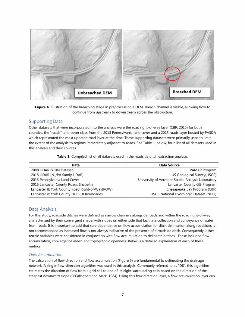
Figure 4. Illustration of the breaching stage in preprocessing a DEM. Breach channel is visible, allowing flow to

continue from upstream to downstream across the obstruction.

Supporting Data Other datasets that were incorporated into the analysis were the road right-of-way layer (CBP, 2015) for both

counties, the “roads” land cover class from the 2013 Pennsylvania land cover and a 2015 roads layer hosted by PASDA

which represented the most updated road layer at the time. These supporting datasets were primarily used to limit

the extent of the analysis to regions immediately adjacent to roads. See Table 1, below, for a list of all datasets used in

this analysis and their sources.

Table 1. Compiled list of all datasets used in the roadside ditch extraction analysis.

Data Data Source

2008 LiDAR & TIN Dataset PAMAP Program

2015 LiDAR (NJ/PA Sandy LiDAR) US Geological Survey(USGS)

2013 Pennsylvania Land Cover University of Vermont Spatial Analysis Laboratory

2015 Lancaster County Roads Shapefile Lancaster County GIS Program

Lancaster & York County Road Right-of-Way(ROW) Chesapeake Bay Program (CBP)

Lancaster & York County HUC-10 Boundaries USGS National Hydrologic Dataset (NHD)

Data Analysis For this study, roadside ditches were defined as narrow channels alongside roads and within the road right-of-way

characterized by their convergent shape, with slopes on either side that facilitate collection and conveyance of water

from roads. It is important to add that sole dependence on flow accumulation for ditch delineation along roadsides is

not recommended as increased flow is not always indicative of the presence of a roadside ditch. Consequently, other

terrain variables were considered in conjunction with flow accumulation to delineate ditches. These included flow

accumulation, convergence index, and topographic openness. Below is a detailed explanation of each of these

metrics.

Flow Accumulation The calculation of flow direction and flow accumulation (Figure 5) are fundamental to delineating the drainage

network. A single-flow-direction algorithm was used in this analysis. Commonly referred to as “D8”, this algorithm

estimates the direction of flow from a grid cell to one of its eight surrounding cells based on the direction of the

steepest downward slope (O’Callaghan and Mark, 1984). Using this flow direction layer, a flow accumulation layer can

8

be created that sums the number of upslope cells that contribute flow to each downslope cell in a raster. Stream

channels and drainage networks can be delineated by applying a threshold to the flow accumulation.

Figure 5. Illustration of outputs from D8 flow direction (left) and unthresholded flow accumulation (right) calculations.

Convergence Index

The convergence index (Figure 6a) is a morphometric variable (Equation 1, below) that relates the aspect of eight

surrounding cells to a center cell. Negative values are indicative of divergent terrain, positive values are indicative of

convergent terrain, and a value of 0 is indicative of a planar surface. The index was calculated in SAGA v4.0 and the

output was given in percentage. The percentage value is a measure of the aspect i.e. the percentage of surrounding

cells pointing to the center cell. This index is calculated using the equation:

Equation 1.

Here θ, is the average slope aspect of the surrounding cells relative to the focal cell. In the context of its functionality,

it is quite similar to planform curvature.

Figure 6. (a) 100% negative convergence (b) 0% even slope (planar surface) (c) 100% positive convergence (Conrad,

2001).

9

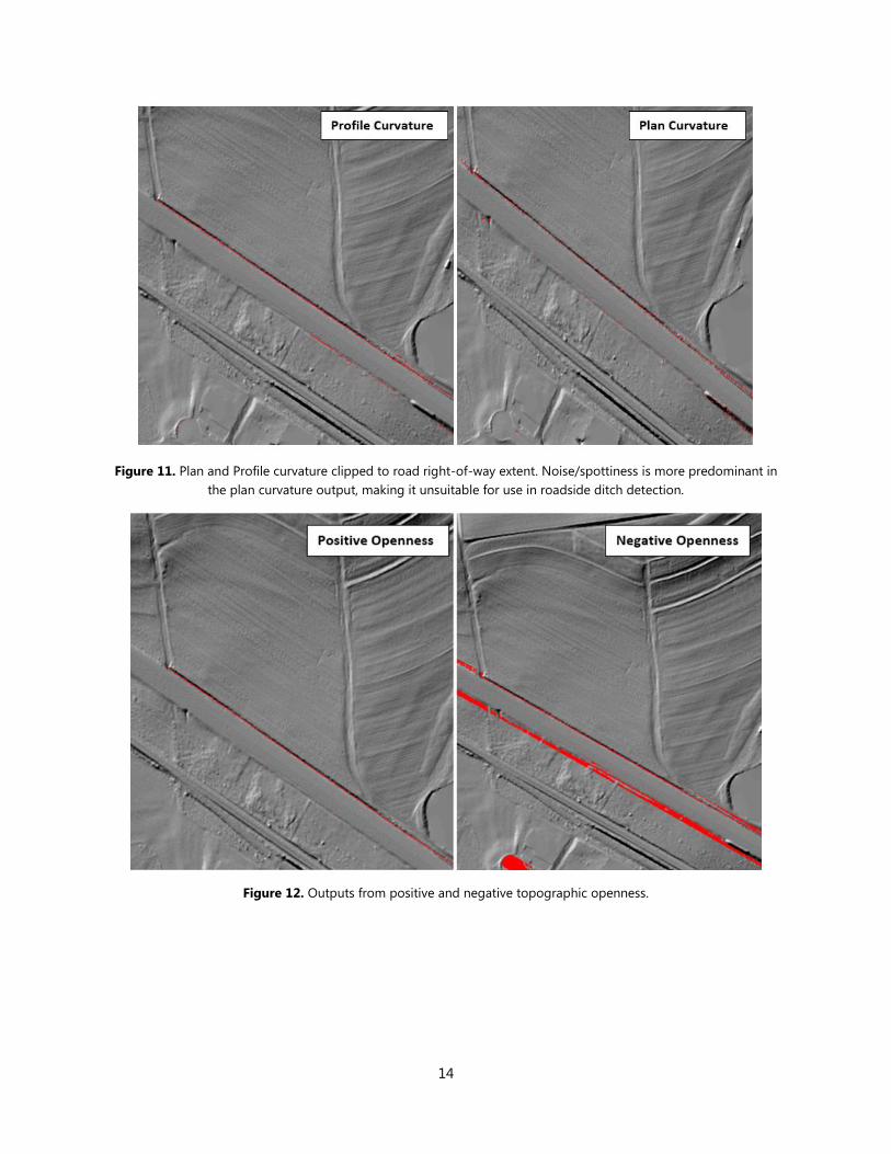
Topographic Openness Topographic openness is a morphometric index that utilizes the line of sight principle to express the degree of

dominance or enclosure of a location on an irregular surface (Yokoyama et al., 2002). Openness is calculated using the

average of the maximum unobstructed viewing angles from a central point within a given radial distance, measured in

eight azimuthal directions. The viewing angle is measured from zenith (i.e. above ground) in the case of positive

openness, or from nadir (i.e. below ground) in the case of negative openness (Figures 7 & 8).

The positive openness, ρ rad, of a location within a specified radius, rad, is calculated as:

Equation 2.

While the negative openness, η rad, within a specified radius is calculated as:

Equation 3.

Figure 7. Illustration of positive openness (left) and negative openness (right) where L is the radial limit of calculation

(Yokoyama et al., 2002).

Figure 8. Illustration of high and low scores for positive and negative openness (Yokoyama et al., 2002).

10

Alternative methods considered To complement the results of the initial analysis, additional terrain variables were investigated. These methods were

not included in the final methodology but were helpful in narrowing down the approaches undertaken. Brief

explanations for these methods are given below because the CIC believes that with more research and more literature

guidance, these methods can be used to improve current ditch mapping efforts. These methods include:

Topographic Wetness Index Topographic wetness index (TWI) is a function that relates specific catchment area and slope of the terrain. The

equation for calculating TWI can be seen below in Equation 4 where α is the catchment area and β is the slope of the

terrain (Beven and Kirby, 1979). TWI can be used to identify areas vulnerable to saturation and liable to produce

surface runoff. In the context of this analysis, TWI was calculated to investigate a possible relationship between

regions with a high wetness index and the presence of ditches in these regions. The hypothesis was that there would

be a positive correlation between regions with high wetness and presence of roadside ditches.

Equation 4.

Profile Curvature Profile Curvature is the rate of change of slope of a surface along the direction of maximum slope. It influences the

flow velocity across the surface. A negative profile curvature indicates the surface is upwardly convex and associated

with increasing flow velocity. A positive profile curvature indicates an upwardly concave surface and represents a

deceleration of flow along the surface. Our hypothesis is that in calculating profile curvature, roadside ditches would

exhibit high positive profile curvature, indicating that the surface of roadside ditches display upward concavity.

Plan Curvature Plan Curvature is the curvature perpendicular to the direction of the maximum slope. Plan curvature is good for

detailing the convergence and divergence of flow across a surface. Positive plan curvature value indicates that the

surface is horizontally convex at the specified cell while a negative value would indicate that the surface is horizontally

concave at the specified cell. A value of zero indicates surface linearity. Plan curvature is beneficial for differentiating

between valleys and ridges. Our hypothesis suggests that using plan curvature will not yield any useful results for

delineating ditches.

Total Curvature Total Curvature is the second derivative of slope. It is the combination of plan and profile curvature and defines the

general curvature of the surface. Positive curvature values represent more convex surfaces, negative curvature values

represent the more concave surfaces such as valleys and zero values are indicative of flat surfaces. Our hypothesis

suggests that ditches will exhibit negative curvature values due to their concave nature.

Terrain Ruggedness Index Terrain Ruggedness Index is an index that expresses the magnitude of elevation difference between contiguous cells

in DEM grid. This index calculates the standard deviation of the adjacent cell values from the central cell. This

approach is good for detecting and measuring and topographic heterogeneity. In measuring the ruggedness index

relative to ditch delineation, it was posited that ditch channels would display similar patterns of terrain heterogeneity

across the landscape.

Terrain Surface Convexity

Terrain Surface Convexity defines the ratio of cells with positive surface curvature values to the total number of cells

within a specified radius. Its basic measurement is similar to that of convergence index, however, the difference is

outlined in its calculation. While the convergence index calculates the general convergence of adjacent cells to the

11

focal cell, the percentage surface convexity is only calculated for cells within the specified radius. Our hypothesis is

that is ditches will display low convexity values which would correspond to high values of concavity.

RESULTS AND DISCUSSION The total length of extracted roadside ditches for the subset of the study area was approximately 34,762 meters (21.6

miles) with an average length of 115 meters (~0.07 miles). The density of ditches per square mile was measured at

0.33 miles of ditches per square mile. The observed density of the roadside ditches in the pilot watershed was highest

around farms or agricultural regions where the land was being drained for crop cultivation. There was not a significant

number of roadside ditches observed within suburban residential regions. Connectivity of roadside ditches to streams

and other waterways was not analyzed. On a county scale, Lancaster County had a total ditch length of approximately

240,247 meters (149 miles) with an average length of 91 meters (~0.06 miles) while York County had a total ditch

length of approximately 277,740 meters (173 miles) with an average length of 88 meters (~0.05 miles). Lancaster

County had a density of approximately 0.15 miles of ditches per square mile while York County had a density of

approximately 0.19 miles of ditches per square mile.

Defining Thresholds In deriving the right threshold values, topographic openness and convergence index were calculated on raw DEMs.

This was done because breaching and pit filling alter the values within the DEM thereby decreasing the likelihood of

detecting geomorphic features needed for delineating roadside ditch channels. Preprocessing the DEM is only

advisable for the calculation of flow direction and flow accumulation because of its function in conditioning the DEM

for hydrologic analysis. All data was subsequently clipped to the road ROW to confine data to the extent of the

analysis. See Table 2 below for a detailed list of threshold values applied to terrain variables.

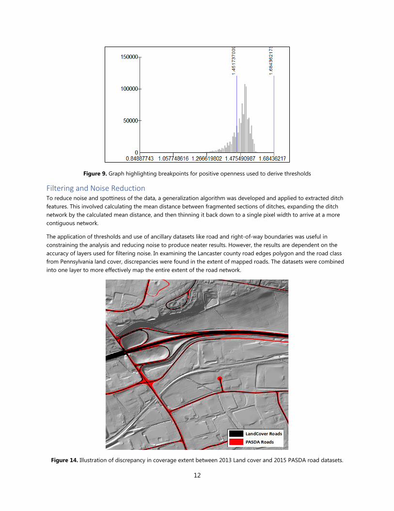
The threshold for positive openness was calculated by the analyzing the distribution of values, identifying a

breakpoint, and rounding to two decimal places (Figure 9). A threshold of 1,000 square meters was applied to the

flow accumulation to delineate the drainage network within the road right-of-way. Using data breakpoints to

establish thresholds was successful at distinguishing statistically homogenous features from dissimilar features within

roadsides. Roadside ditches in this case were assumed to have homogeneous characteristics that distinguish them

from other ground features along road edges.

Roadside ditches were estimated to exist between features on road edges that exhibited -75% and -25%

convergence. The ditches mapped exhibited negative convergence indicating that values surrounding the center cells

(ditches) were of higher elevation values, which followed this project’s definition for roadside ditches. The results

suggest that the development of thresholds was effective in extracting ditch extents as well as their orientation.

Table 2. Table detailing threshold values of variables used in delineating roadside ditches

Variables Threshold Values Units

Flow Accumulation ≥ 1000 Square meters

Convergence Index -75 ≤ CI ≥ -25 Percent

Positive Openness ≤ 1.45 Radians

12

Figure 9. Graph highlighting breakpoints for positive openness used to derive thresholds

Filtering and Noise Reduction To reduce noise and spottiness of the data, a generalization algorithm was developed and applied to extracted ditch

features. This involved calculating the mean distance between fragmented sections of ditches, expanding the ditch

network by the calculated mean distance, and then thinning it back down to a single pixel width to arrive at a more

contiguous network.

The application of thresholds and use of ancillary datasets like road and right-of-way boundaries was useful in

constraining the analysis and reducing noise to produce neater results. However, the results are dependent on the

accuracy of layers used for filtering noise. In examining the Lancaster county road edges polygon and the road class

from Pennsylvania land cover, discrepancies were found in the extent of mapped roads. The datasets were combined

into one layer to more effectively map the entire extent of the road network.

Figure 14. Illustration of discrepancy in coverage extent between 2013 Land cover and 2015 PASDA road datasets.

13

Contiguous groups of cells comprising each roadside ditch channel were then analyzed individually. Channel statistics

were calculated to derive the mean length, minimum length, maximum length and standard deviation of all identified

channels. All ditch channels with lengths less than the average length calculated were excluded from the final ditch

data inventory. This was done under the assumption that extracted channels less than the mean length are more likely

to be a result of noise rather than actual roadside ditches (Figure 10). The final dataset was converted to a polyline,

smoothed, and filtered to remove any ditches which were visually determined to be inaccurate.

Figure 10. Illustration of average length criteria used to distinguish ditches from noise

Exclusion of Alternative Methods

The results of the alternative methods described above were not conclusive enough to be factored into the results

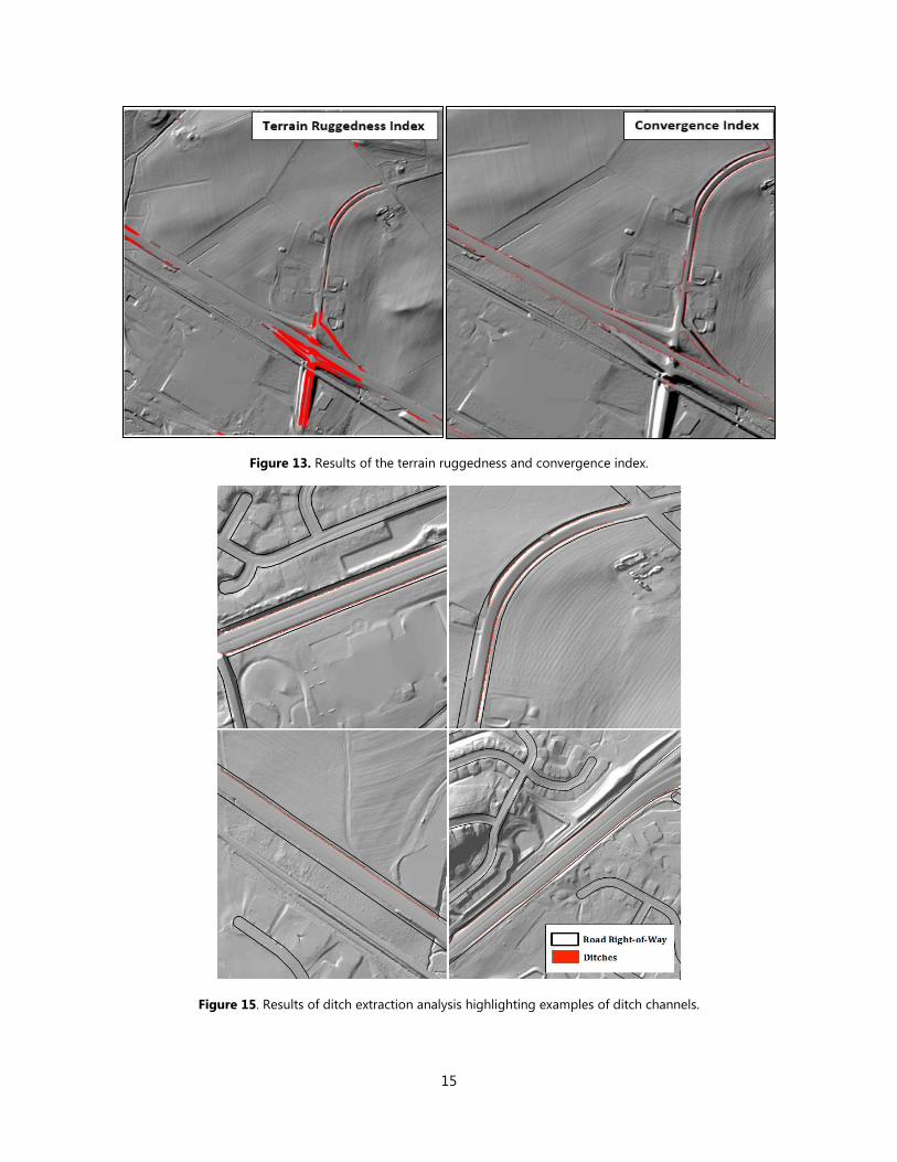
dataset. Curvature and ruggedness indices produced spotty data that, when compared side-by-side with openness,

did not provide significant improvements to the final dataset. See Figures 11 through 13 below for a comparison of

different terrain variables and datasets used.

14

Figure 11. Plan and Profile curvature clipped to road right-of-way extent. Noise/spottiness is more predominant in

the plan curvature output, making it unsuitable for use in roadside ditch detection.

Figure 12. Outputs from positive and negative topographic openness.

15

Figure 13. Results of the terrain ruggedness and convergence index.

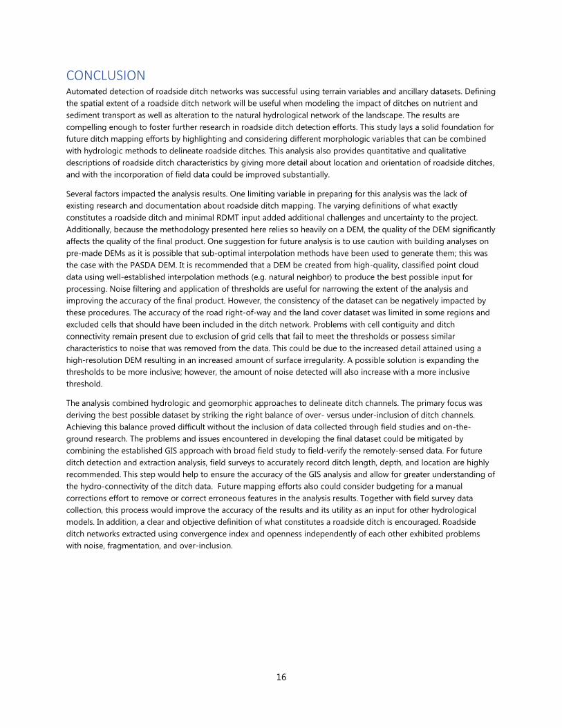
Figure 15. Results of ditch extraction analysis highlighting examples of ditch channels.

16

CONCLUSION Automated detection of roadside ditch networks was successful using terrain variables and ancillary datasets. Defining

the spatial extent of a roadside ditch network will be useful when modeling the impact of ditches on nutrient and

sediment transport as well as alteration to the natural hydrological network of the landscape. The results are

compelling enough to foster further research in roadside ditch detection efforts. This study lays a solid foundation for

future ditch mapping efforts by highlighting and considering different morphologic variables that can be combined

with hydrologic methods to delineate roadside ditches. This analysis also provides quantitative and qualitative

descriptions of roadside ditch characteristics by giving more detail about location and orientation of roadside ditches,

and with the incorporation of field data could be improved substantially.

Several factors impacted the analysis results. One limiting variable in preparing for this analysis was the lack of

existing research and documentation about roadside ditch mapping. The varying definitions of what exactly

constitutes a roadside ditch and minimal RDMT input added additional challenges and uncertainty to the project.

Additionally, because the methodology presented here relies so heavily on a DEM, the quality of the DEM significantly

affects the quality of the final product. One suggestion for future analysis is to use caution with building analyses on

pre-made DEMs as it is possible that sub-optimal interpolation methods have been used to generate them; this was

the case with the PASDA DEM. It is recommended that a DEM be created from high-quality, classified point cloud

data using well-established interpolation methods (e.g. natural neighbor) to produce the best possible input for

processing. Noise filtering and application of thresholds are useful for narrowing the extent of the analysis and

improving the accuracy of the final product. However, the consistency of the dataset can be negatively impacted by

these procedures. The accuracy of the road right-of-way and the land cover dataset was limited in some regions and

excluded cells that should have been included in the ditch network. Problems with cell contiguity and ditch

connectivity remain present due to exclusion of grid cells that fail to meet the thresholds or possess similar

characteristics to noise that was removed from the data. This could be due to the increased detail attained using a

high-resolution DEM resulting in an increased amount of surface irregularity. A possible solution is expanding the

thresholds to be more inclusive; however, the amount of noise detected will also increase with a more inclusive

threshold.

The analysis combined hydrologic and geomorphic approaches to delineate ditch channels. The primary focus was

deriving the best possible dataset by striking the right balance of over- versus under-inclusion of ditch channels.

Achieving this balance proved difficult without the inclusion of data collected through field studies and on-the-

ground research. The problems and issues encountered in developing the final dataset could be mitigated by

combining the established GIS approach with broad field study to field-verify the remotely-sensed data. For future

ditch detection and extraction analysis, field surveys to accurately record ditch length, depth, and location are highly

recommended. This step would help to ensure the accuracy of the GIS analysis and allow for greater understanding of

the hydro-connectivity of the ditch data. Future mapping efforts also could consider budgeting for a manual

corrections effort to remove or correct erroneous features in the analysis results. Together with field survey data

collection, this process would improve the accuracy of the results and its utility as an input for other hydrological

models. In addition, a clear and objective definition of what constitutes a roadside ditch is encouraged. Roadside

ditch networks extracted using convergence index and openness independently of each other exhibited problems

with noise, fragmentation, and over-inclusion.

17

REFERENCES Abdel-Fattah, M., Saber, M., Kantoush, S. A., Khalil, M. F., Sumi, T., & Sefelnasr, A. M. (2017). A Hydrological and

Geomorphometric Approach to Understanding the Generation of Wadi Flash Floods. Water, 9(7), 553.

Beven, K. J., & Kirkby, M. J. (1979). A physically based, variable contributing area model of basin hydrology/Un modèle

à base physique de zone d'appel variable de l'hydrologie du bassin versant. Hydrological Sciences Journal, 24(1), 43-

69.

Buchanan, B. P., Falbo, K., Schneider, R. L., Easton, Z. M., & Walter, M. T. (2012). Hydrological impact of roadside

ditches in an agricultural watershed in Central New York: implications for non‐point source pollutant transport.

Hydrological processes, 27(17), 2422-2437.

Buchanan, B., Easton, Z. M., Schneider, R. L., & Walter, M. T. (2013). Modeling the hydrologic effects of roadside ditch

networks on receiving waters. Journal of hydrology, 486, 293-305.

Falbo, K., Schneider, R. L., Buckley, D. H., Walter, M. T., Bergholz, P. W., & Buchanan, B. P. (2013). Roadside ditches as

conduits of fecal indicator organisms and sediment: Implications for water quality management. Journal of

environmental management, 128, 1050-1059.

Heidemann, H. K. (2012). Lidar base specification (No. 11-B4). US Geological Survey.

James, L. A., Watson, D. G., & Hansen, W. F. (2007). Using LiDAR data to map gullies and headwater streams under

forest canopy: South Carolina, USA. Catena, 71(1), 132-144.

Kiss, R. (2004). Determination of drainage network in digital elevation models, utilities and limitations. Journal of

Hungarian Geomathematics, 2, 16-29.

Ledoux, H., & Gold, C. (2005). An efficient natural neighbour interpolation algorithm for geoscientific modelling.

Developments in spatial data handling, 97-108.

Liu, X., & Zhang, Z. (2011). Drainage network extraction using LiDAR‐derived DEM in volcanic plains. Area, 43(1), 42-

52.

O'Callaghan, J. F., & Mark, D. M. (1984). The extraction of drainage networks from digital elevation data. Computer

vision, graphics, and image processing, 28(3), 323-344.

Passalacqua, P., Belmont, P., & Foufoula‐Georgiou, E. (2012). Automatic geomorphic feature extraction from lidar in

flat and engineered landscapes. Water Resources Research, 48(3).

Pirotti, F., & Tarolli, P. (2010). Suitability of LiDAR point density and derived landform curvature maps for channel

network extraction. Hydrological Processes, 24(9), 1187-1197.

Rapinel, S., Hubert-Moy, L., Clément, B., Nabucet, J., & Cudennec, C. (2015). Ditch network extraction and

hydrogeomorphological characterization using LiDAR-derived DTM in wetlands. Hydrology Research, 46(2), 276-290.

Sofia, G., Tarolli, P., Cazorzi, F., & Dalla Fontana, G. (2011). An objective approach for feature extraction: distribution

analysis and statistical descriptors for scale choice and channel network identification. Hydrology and earth system

sciences, 15(5), 1387.

Walker, J. P., & Willgoose, G. R. (1999). On the effect of digital elevation model accuracy on hydrology and

geomorphology. Water Resources Research, 35(7), 2259-2268.

Yokoyama, R., Shirasawa, M., & Pike, R. J. (2002). Visualizing topography by openness: a new application of image

processing to digital elevation models. Photogrammetric engineering and remote sensing, 68(3), 257-266.