liens code de la propriété intellectuelle. articles l 122....
TRANSCRIPT

AVERTISSEMENT
Ce document est le fruit d'un long travail approuvé par le jury de soutenance et mis à disposition de l'ensemble de la communauté universitaire élargie. Il est soumis à la propriété intellectuelle de l'auteur. Ceci implique une obligation de citation et de référencement lors de l’utilisation de ce document. D'autre part, toute contrefaçon, plagiat, reproduction illicite encourt une poursuite pénale. Contact : [email protected]
LIENS Code de la Propriété Intellectuelle. articles L 122. 4 Code de la Propriété Intellectuelle. articles L 335.2- L 335.10 http://www.cfcopies.com/V2/leg/leg_droi.php http://www.culture.gouv.fr/culture/infos-pratiques/droits/protection.htm
Université de Lorraine
Thèsepour obtenir le grade de :
Docteur de l’Université de Lorraine
dans la spécialité
Physique
par
Nicolas Allegra
Propriétés critiques des modèles de dimères, de
chaînes de spin et d’interfaces
Critical Properties of Dimers, Spin chains and
Interface Models
Thèse soutenue le 29 septembre 2015 devant le jury composé de :
M. Philippe Ruelle Professeur, Université Catholique de Louvain Président du jury
M. Jesper Jacobsen Professeur, Université Pierre et Marie Curie Rapporteur
M. Herbert Spohn Professeur, Technical University Munich Rapporteur
M. Kay Wiese Directeur de Recherche CNRS, LPTENS Examinateur
M. Gregory Schehr Chargé de Recherche CNRS, LPTMS Examinateur
M. Malte Henkel Professeur, Université de Lorraine Directeur de Thèse
M. Jean-Yves Fortin Directeur de Recherche CNRS, IJL Co-Directeur de Thèse
Institut Jean Lamour
Faculté des Sciences et Technologies
F-54506 VANDOEUVRE les NANCY cedex France
Université de Lorraine

Remerciements
Tout d’abord, je tiens à remercier Malte pour avoir accepté d’être mon directeur de thèse et de m’avoirtant appris durant ces trois années. Cette thèse témoigne de sa double compétence en physique statistiqueà l’équilibre et hors de l’équilibre. Je le remercie de m’avoir permis de travailler sur divers sujets et ainside m’écarter du sujet initial tout en gardant un oeil bienveillant sur moi. Je le remercie aussi pour toutesces discussions quotidiennes de physique et autres et de m’avoir soutenu quotidiennement. Mes secondsremerciements vont naturellement envers Jean-Yves qui est rapidement devenu mon second directeur dethèse et avant tout mon ami, malgré notre fondamentale divergence VTT / Vélo de route. Je le remercied’avoir supporté ma présence journalière dans son bureau, de m’avoir permis d’aller à Séoul, de m’avoirappris tant de choses et surtout d’avoir été présent durant ces trois années.
Je tiens ensuite à remercier mes deux rapporteurs Herbert Spohn et Jesper Jacobsen d’avoiraccepté de lire ma thèse et d’assister à la soutenance. Je les remercie aussi pour les discussions que j’ai puavoir avec eux à Paris, aux Houches, à Florence et ailleurs. J’en profite pour remercier Jesper pour soncours de M2 à Paris que j’ai particulièrement apprécié et qui m’a tant servi pendant ces années de thèse.Je remercie également Kay Wiese et Grégory Schehr pour avoir été examinateurs de cette thèse, ce fut ungrand plaisir de les avoir dans mon jury. Je remercie aussi ce dernier pour la parfaite organisation de l?écoledes Houches l’été dernier où j’ai pu écrire une bonne partie de cette thèse dans un cadre exceptionnel.Un grand merci à Philippe Ruelle de m’avoir fait l’honneur de présider ce jury et de m’avoir invité àLouvain où j’ai pu apprécier la fameuse hospitalité belge. Finalement, un mot de remerciements auxexcellents professeurs que j’ai eu la chance d’avoir tout au long de ces années et je suis particulièrementreconnaissant envers Jérôme Léon qui a su me donner le goût de la recherche en physique.
Ces trois années à Nancy n’auraient pas été les mêmes sans la présence de tous les membresdu groupe. Je pense en premier à Christophe avec qui j’ai tant discuté, appris et même couru. Si c’étaità refaire, je ferais volontiers une thèse avec toi. Merci à Bertrand pour m’avoir permis de voyager plusque je ne l’aurai rêvé et de s’être toujours intéressé à mes recherches. Je n’ai ni la place, ni la patiencede remercier les membres du groupe un à un mais je tiens à remercier Loïc pour m’avoir beaucoup aidéet de m’avoir toujours donné les bonnes références. Rapidement, mes remerciements vont aussi enversAlexandre, Dragi, Olivier, Thierry, Gunnar et bien-sûr Jérôme avec qui j’ai pu travailler dans ma dernièreannée. Je le remercie pour ses explications claires et précises, ainsi que pour ses nombreux conseils. J’enprofite pour remercier les deux autres membres de la communauté du cercle arctique, Jean- Marie etJacopo pour cette collaboration incroyablement intéressante. Je remercie aussi Laurent Chaput et JérémieUnterberger pour diverses discussions et conseils ainsi que toutes les personnes avec qui j’ai pu échangerau cours de mes voyages, je pense notamment à Masayuki Hase et Segun Goh.
Une thèse n’en serait pas vraiment une sans la présence d’autres thésards. Je pense tout d’abord
à Sophie avec qui j’ai tant partagé et qui a réussi à venir à ma soutenance malgré un emploi du temps
chargé. Merci aussi à Pierre, Dimitri, Hugo, Mariana, Nelson, Emilio, Sasha et Xavier pour la bonne
ambiance dans notre bureau. Je remercie aussi Thimothée d’être venu de Paris pour ma soutenance et
Thomas et mes autres camarades de classe pour tous ces moments avant la thèse. Evidemment, tous mes
amis hors de la physique sont aussi remerciés et ils se reconnaitront si jamais ils tombent sur ces lignes.
Pour finir, mes remerciements les plus profonds vont vers ma famille et surtout mes parents qui m’ont
toujours soutenu et qui m’ont permis d’être là où je suis aujourd’hui.
2
CONTENTS
Contents
I Critical properties of 2d dimer models and related c = 1 CFT’s 6
1 Some properties of 2d critical systems and dimer models 7
1.1 Introduction to lattice models and dimers . . . . . . . . . . . . . . . . . . . . . . . 8
1.1.1 Ising model and graph expansion . . . . . . . . . . . . . . . . . . . . . . . . 8
1.1.2 From Grassmann algebra to dimer models . . . . . . . . . . . . . . . . . . . 10
1.1.3 Local statistics and non-local properties . . . . . . . . . . . . . . . . . . . . 18
1.2 Relation to other statistical models . . . . . . . . . . . . . . . . . . . . . . . . . . . 21
1.2.1 Back to Ising . . . . . . . . . . . . . . . . . . . . . . . . . . . . . . . . . . . 21
1.2.2 Temperley bijection and spanning trees . . . . . . . . . . . . . . . . . . . . 22
1.2.3 From dimer covering to edge coloring . . . . . . . . . . . . . . . . . . . . . . 23
1.3 About the full monomer-dimer model . . . . . . . . . . . . . . . . . . . . . . . . . 25
1.3.1 Mean-field approximation . . . . . . . . . . . . . . . . . . . . . . . . . . . . 26
1.3.2 Baxter approach and matrix product state . . . . . . . . . . . . . . . . . . 28
1.3.3 Heilmann-Lieb theorem and Ising model in a magnetic field . . . . . . . . . 31
1.4 Conclusions . . . . . . . . . . . . . . . . . . . . . . . . . . . . . . . . . . . . . . . . 33
2 Dimer model: Plechko solution and generalization 34
2.1 Plechko solution . . . . . . . . . . . . . . . . . . . . . . . . . . . . . . . . . . . . . 35
2.1.1 Fermionization and mirror symmetry . . . . . . . . . . . . . . . . . . . . . . 35
2.1.2 Pfaffian solution without monomer . . . . . . . . . . . . . . . . . . . . . . . 36
2.1.3 Majorana fermions lattice theory . . . . . . . . . . . . . . . . . . . . . . . . 39
2.2 Pfaffian solution with 2n monomers . . . . . . . . . . . . . . . . . . . . . . . . . . 41
2.2.1 General solution of the problem . . . . . . . . . . . . . . . . . . . . . . . . . 42
2.2.2 Boundary monomers and 1d complex fermion chain . . . . . . . . . . . . . 48
2.2.3 Single monomer on the boundary and localization phenomena . . . . . . . . 52
2.3 Fun with dimers . . . . . . . . . . . . . . . . . . . . . . . . . . . . . . . . . . . . . 54
2.3.1 Partition function without monomers . . . . . . . . . . . . . . . . . . . . . 54
3

CONTENTS
2.3.2 Partition function with two boundary monomers . . . . . . . . . . . . . . . 55
2.3.3 Partition function with 2n boundary monomers . . . . . . . . . . . . . . . . 57
2.4 Conclusions of the chapter . . . . . . . . . . . . . . . . . . . . . . . . . . . . . . . . 58
3 CFT analysis of the 2d dimer model 59
3.1 Bosonic theory and boundary conditions . . . . . . . . . . . . . . . . . . . . . . . . 60
3.1.1 Height mapping and Coulomb gas formalism . . . . . . . . . . . . . . . . . 60
3.1.2 A few word about conformal field theory in the plane . . . . . . . . . . . . 62
3.1.3 Rectangular geometry and boundary conditions . . . . . . . . . . . . . . . 62
3.2 Dimer models in various geometries . . . . . . . . . . . . . . . . . . . . . . . . . . . 64
3.2.1 Boundary CFT and conformal mapping . . . . . . . . . . . . . . . . . . . . 64
3.2.2 CFT on a rectangle and corner free energy . . . . . . . . . . . . . . . . . . 65
3.2.3 Transfer matrix formulation and CFT on a infinite strip . . . . . . . . . . . 70
3.3 Scaling behavior of monomer and dimer correlation functions . . . . . . . . . . . . 74
3.3.1 Boundary conformal dimensions . . . . . . . . . . . . . . . . . . . . . . . . 74
3.3.2 Monomer correlations . . . . . . . . . . . . . . . . . . . . . . . . . . . . . . 74
3.3.3 Dimer correlations and composite particles . . . . . . . . . . . . . . . . . . 78
3.4 Conclusions and perspectives . . . . . . . . . . . . . . . . . . . . . . . . . . . . . . 82
4 Field theory formulation of the arctic circle 83
4.1 The Aztec diamond dimer model . . . . . . . . . . . . . . . . . . . . . . . . . . . . 84
4.1.1 Introduction and generalities . . . . . . . . . . . . . . . . . . . . . . . . . . 84
4.1.2 Height mapping and scalar field theory . . . . . . . . . . . . . . . . . . . . . 86
4.1.3 Transfer matrix formulation . . . . . . . . . . . . . . . . . . . . . . . . . . . 89
4.2 Classical 2d systems and 1d quantum interpretation . . . . . . . . . . . . . . . . . 91
4.2.1 6-vertex model and DWBC . . . . . . . . . . . . . . . . . . . . . . . . . . . 91
4.2.2 The transfer matrix . . . . . . . . . . . . . . . . . . . . . . . . . . . . . . . 93
4.2.3 Fermionic chain with a generic dispersion relation . . . . . . . . . . . . . . 95
4.3 Arctic field theory . . . . . . . . . . . . . . . . . . . . . . . . . . . . . . . . . . . . 102
4.3.1 Exact correlation functions . . . . . . . . . . . . . . . . . . . . . . . . . . . 102
4.3.2 Long-range correlations . . . . . . . . . . . . . . . . . . . . . . . . . . . . . 105
4.3.3 Dirac field theory in curved space . . . . . . . . . . . . . . . . . . . . . . . . 107
4.4 Conclusions . . . . . . . . . . . . . . . . . . . . . . . . . . . . . . . . . . . . . . . . 110
5 Résumé en français de la partie I 111
4

CONTENTS
II Critical properties of interface growth models 119
6 Introduction to interface: Markov processes and scaling behavior 120
6.1 Markov formalism . . . . . . . . . . . . . . . . . . . . . . . . . . . . . . . . . . . . 121
6.1.1 Interface as a stochastic process . . . . . . . . . . . . . . . . . . . . . . . . . 121
6.1.2 From a master equation to a Fokker-Planck equation . . . . . . . . . . . . . 122
6.1.3 Langevin equation . . . . . . . . . . . . . . . . . . . . . . . . . . . . . . . . 122
6.2 Interface growth process with diffusion . . . . . . . . . . . . . . . . . . . . . . . . . 123
6.2.1 Deposition-relaxation processes . . . . . . . . . . . . . . . . . . . . . . . . . 123
6.2.2 Restricted solid on solid processes . . . . . . . . . . . . . . . . . . . . . . . 125
6.2.3 Other processes and universality classes . . . . . . . . . . . . . . . . . . . . 127
6.3 Critical behavior . . . . . . . . . . . . . . . . . . . . . . . . . . . . . . . . . . . . . 128
6.3.1 Langevin equation and scaling properties . . . . . . . . . . . . . . . . . . . 128
6.3.2 Field theory formalism and ageing phenomena . . . . . . . . . . . . . . . . 130
6.3.3 KPZ equation . . . . . . . . . . . . . . . . . . . . . . . . . . . . . . . . . . . 131
7 Boundary interface growth processes 133
7.1 Interface growth near a boundary . . . . . . . . . . . . . . . . . . . . . . . . . . . . 134
7.1.1 Introduction to the problem . . . . . . . . . . . . . . . . . . . . . . . . . . . 134
7.1.2 Deposition-relaxation process with a boundary . . . . . . . . . . . . . . . . 135
7.1.3 Continuum Langevin equation . . . . . . . . . . . . . . . . . . . . . . . . . 137
7.2 Exact solution of the model and numerical comparison . . . . . . . . . . . . . . . . 138
7.2.1 Laplace transform and exact solution . . . . . . . . . . . . . . . . . . . . . . 139
7.2.2 Mean profile of the interface . . . . . . . . . . . . . . . . . . . . . . . . . . . 142
7.2.3 Fluctuation of the height of the interface . . . . . . . . . . . . . . . . . . . 145
7.3 Boundary KPZ equation . . . . . . . . . . . . . . . . . . . . . . . . . . . . . . . . . 151
7.3.1 Introduction and definition of the problem . . . . . . . . . . . . . . . . . . . 152
7.3.2 KPZ equation with a boundary . . . . . . . . . . . . . . . . . . . . . . . . . 153
7.3.3 Scaling hypothesis and numerical results . . . . . . . . . . . . . . . . . . . . 153
7.4 Conclusions . . . . . . . . . . . . . . . . . . . . . . . . . . . . . . . . . . . . . . . . 156
8 Résumé en français de la partie II 157
Bibliography 173
5

PARTICritical properties of 2d dimer models and
related c = 1 CFT’s
6
CHAPTER 1. SOME PROPERTIES OF 2D CRITICAL SYSTEMS AND DIMER MODELS
CHAPTER1Some properties of 2d critical systems and dimer
models
Contents
1.1 Introduction to lattice models and dimers . . . . . . . . . . . . . . . 8
1.1.1 Ising model and graph expansion . . . . . . . . . . . . . . . . . . . . . . 8
1.1.2 From Grassmann algebra to dimer models . . . . . . . . . . . . . . . . . 10
1.1.3 Local statistics and non-local properties . . . . . . . . . . . . . . . . . . 18
1.2 Relation to other statistical models . . . . . . . . . . . . . . . . . . . 21
1.2.1 Back to Ising . . . . . . . . . . . . . . . . . . . . . . . . . . . . . . . . . 21
1.2.2 Temperley bijection and spanning trees . . . . . . . . . . . . . . . . . . 22
1.2.3 From dimer covering to edge coloring . . . . . . . . . . . . . . . . . . . . 23
1.3 About the full monomer-dimer model . . . . . . . . . . . . . . . . . . 25
1.3.1 Mean-field approximation . . . . . . . . . . . . . . . . . . . . . . . . . . 26
1.3.2 Baxter approach and matrix product state . . . . . . . . . . . . . . . . 28
1.3.3 Heilmann-Lieb theorem and Ising model in a magnetic field . . . . . . . 31
1.4 Conclusions . . . . . . . . . . . . . . . . . . . . . . . . . . . . . . . . . . 33
7

CHAPTER 1. SOME PROPERTIES OF 2D CRITICAL SYSTEMS AND DIMER MODELS
This chapter is mainly a review of basic knowledge and personal views about the classicaldimer model in the framework of 2d classical phenomena. The field of lattice statistical physics isexemplified by the so-called high-temperature expansion of the square lattice Ising model leading toa pure combinatorial problem very similar to the one we will be interested in. Then, by introducingGrassmann algebra we shall see how to define and express the partition function of the dimer modelin a fermionic framework. After a rapid survey of the standard Kasteleyn solution and its mainapplications, some of the most interesting relations to other combinatorial problems are presentedin a quite pedestrian way. The third part of this chapter is dedicated to the so-called monomer-dimer model, which turns out to be more complicated to study. We will see how to extract someinformations about the phases using in one hand a mean-field method and in another hand asophisticated transfer matrix approach which leads to the famous result about the absence ofphase transition, and which can be proved rigorously as we shall see at the end of the chapter.
1.1 Introduction to lattice models and dimers
Lattice models has always played a great role in the history of physics when it comes to thedescription of the phases of matter, mainly because of the intrinsic nature of the microscopic world.Following Onsager’s solution of the 2d Ising model in the forties [165, 122, 123], the introductionof the Bethe ansatz [20] and the discovery of the machinery of transfer matrices, the field of exactsolutions of lattice statistical physics models has exploded leading to the birth of a new field oftheoretical and mathematical physics known as exactly solved models [17]. The confluence of thisnew field with 2d conformal field theory [18] discovered by Belavin, Polyakov and Zamolodchikov
(see [56] for an extensive monography) had a huge impact in theoretical physics, from high energyto condensed matter, leading to a whole new level of understanding of classical and quantumintegrable systems [141]. In the next few pages, we will explore a few properties of different latticemodels that I find relevant for the discussion to come.
1.1.1 Ising model and graph expansion
We shall start our discussion about statistical lattice models and relation to some combinatorialproblems, examining a particular combinatorial solution of the ferromagnetic Ising model intro-duced by Lenz and Ising, with the following hamiltonian
H = −J∑
〈ij〉
sisj . (1.1)
The exact computation of the partition function of this model in 2d was started by Onsager[165, 122, 123] in the forties and led to a rather good understanding of the phase diagram of themodel (see Fig. 1.2). Another approach to compute, in an exact way, the partition function is towrite down explicitly how the latter can be expand around some specific temperature values, i.e.in the limit of low or high temperature. Kramers and Wannier were able to show that the hightemperature expansion and the low temperature expansion of the model are equivalent up to anoverall rescaling of the free energy, under the restricted assumption that there is only one criticalpoint in between. In the following we will briefly explain how this expansion can be performed
8

CHAPTER 1. SOME PROPERTIES OF 2D CRITICAL SYSTEMS AND DIMER MODELS
β = 0 β = ∞βc
Figure 1.1: (a) Phase diagram of the 2d ferromagnetic Ising model with free boundary conditions.The point β = ∞ correspond to the ferromagnetic phase and the point β = 0 correspond to thedisordered phase around our high-temperature expansion is performed separated by a critical pointat βc = ln(1 +
√2)/2, which can be found exactly using the Kramers-Wannier duality.
in the high temperature limit, for the case of the 2d Ising model on the square lattice1. Here weexpect the partition function to be dominated by the completely random, disordered configurationsof maximum entropy. Our goal is to find a way to expand the partition function in βJ ≪ 1.
Z =∑
{s}
exp(
βJ∑
〈ij〉
sisj
)
=∑
{s}
∏
〈ij〉
exp (βJsisj). (1.2)
There is a useful way to rewrite exp (βJsisj) which relies on the fact that the product sisj onlytakes value ±1. It does not take long to check the following identity
exp (βJsisj) = a(1 + bsisj), (1.3)
with a = cosh βJ and b = tanh βJ . Using this graph expansion, we can write the partitionfunction as the sum over all the configurations of polygons. A graphical representation can beassociated with the expansion of the product as follows. We color any given edge if the term bsisj
Z = + + + + O(b10)
is taken, and leave the edge empty if we take the term 1. The contribution of graphs in which anyvertex is incident on an odd number of colored edges then vanishes upon taking the sum over spinconfigurations. In other words, non-zero contributions correspond to graphs consisting of closedpolygons and the partition function reads
Z =∑
{s}
∏
〈ij〉
exp (βJsisj) = a2V∑
{s}
∏
〈ij〉
(1 + bsisj)). (1.4)
This is often referred to as a high-temperature expansion, since tanh βJ ≪ 1 when βJ ≪ 1, but
1This method is quite generic and can be extended for a lot of models in any dimensions
9

CHAPTER 1. SOME PROPERTIES OF 2D CRITICAL SYSTEMS AND DIMER MODELS
Figure 1.2: The list of all 512 loop configurations for the 4× 4 Ising partition function Eq. (1.4)without periodic boundary conditions. I thank Pr Werner Krauth for sharing his code with me.
we stress that this is an exact rewriting of Z that holds for any β. With a lot of hard work onecan estimate behavior of thermodynamic functions from these series. In particular one can seesingularities in the free energy, indicative of a phase transition, and even estimate the behaviornear the singularities. A similar high temperature expansion can also be done for spin correlations.
1.1.2 From Grassmann algebra to dimer models
Grassmann variables [19], thanks to their nilpotent properties, are very suitable to tackle combina-torial lattice models, and many of this models has been partially or entirely solved in the frame offermionic field theory and the dimer model was one of them [184, 185]. In this context, we shouldmention the study of spanning trees and spanning forests [36, 35] as well as the edge-coloringproblem [74, 75] which is a special case of a more general loop model [110, 135]. A n-dimensionalGrassmann algebra 2 is the algebra generated by a set of variables {ai}, with i = 1...n satisfying
{ai, aj} = 0, (1.5)
i.e. they anti-commute, which implies in particular that a2i = 0. The algebra generated by these
quantities contains all expressions of the form
f(a) = f (0) +∑
i
f iai +∑
i<j
f ijaiaj + ..
=∑
06p6n
∑
i
1
p!f i1...ipai1ai2 ...aip , (1.6)
2The presentation closely follows [98].
10
CHAPTER 1. SOME PROPERTIES OF 2D CRITICAL SYSTEMS AND DIMER MODELS
where the coefficients are antisymmetric tensors with p indices, each ranging from 1 to n. Sincethere are
(
np
)
such linearly independent tensors, summing over p from 0 to n produces a 2n-dimensional algebra. The anticommuting rule allows us to define an associative product
f1(a)f2(a) = f01 f
01 +
∑
i
(f01 f
i2 + f i1f
02 )ai +
1
2
∑
ij
(f ij1 f02 + f i1f
j2 − f j1f i2 + f0
1 fij2 )aiaj + .. (1.7)
Please note that in general fg is not equal to ±gf . Nevertheless the subalgebra containing termswith an even number (possibly zero) of a variables commutes with any element f . Having definedsum and products in the Grassmann algebra we now define a left derivative ∂i := ∂ai
. Thederivative gives zero on a monomial which does not contain the variable ai. If the monomialdoes contain ai, it is moved to the left (with the appropriate sign due to the exchanges) and thensuppressed. The operation is extended by linearity to any element of the algebra. A right derivativecan be defined similarly. From this definition the following rules can be obtained
{∂i, ∂j} = 0
{∂i, aj} = δij . (1.8)
Integrals are defined as linear operations over the functions f with the property that they can beidentified with the (left) derivatives [19]. Correspondingly
∫
dai f(a) = ∂if(a),
∫
dai daj f(a) = ∂i∂jf(a), (1.9)
which leads to the generalization∫
daik daik−1...dai1 f(a) = ∂ik∂ik−1
...∂i1f. (1.10)
It is obvious that this definition fulfills the constraint of translational invariance (C,D constant)
∫
da1(C +Da1) =
∫
da1[C +D(a1 + a2)], (1.11)
which requires∫
dai aj = δij . (1.12)
Quadratic and quartic form
Changes of coordinates are required to preserve the anti-commuting structure of the Grassmannalgebra, this allows non-singular linear transformations of the form bi =
∑
j Aijai. One then canverify that by setting f(a) = F (b) one can obtain the following relation
∫
∏
i
dan...da1f(a) = detA
∫
∏
i
dbn...db1F (b), (1.13)
11

CHAPTER 1. SOME PROPERTIES OF 2D CRITICAL SYSTEMS AND DIMER MODELS
at variance with the commuting case in which the factor on the right hand side would have beendet−1 A. We note
∫
D[a, a] =∫∏
i dai dai the Grassmann measure. In the multidimensionalintegral, the symbols da1, ...,daN are again anticommuting with each other. The basic expressionof the Grassmann analysis concern the Gaussian fermionic integrals [184] which is related to thedeterminant
detA =
∫
D[a, a] exp(
N∑
i,j=1
aiAij aj
)
, (1.14)
where {ai, ai} is a set of completely anticommuting Grassmann variables, the matrix in the expo-nential is arbitrary. The two Grassmann variables ai and ai are independent and not conjugate toeach other, they can been seen as composante of a complex Grassmann variables. The Gaussianintegral of the second kind is related to the Pfaffian of the associated skew-symmetric matrix
pfA =
∫
D[a] exp(1
2
N∑
i,j=1
aiAijaj
)
. (1.15)
The pfaffian form is a combinatorial polynomial in Aij , known in mathematics for a long time.The pfaffian and determinant of the associated skew-symmetric matrix are algebraically relatedby detA = (pfA)2. This relation can be most easily proved in terms of the fermionic integrals.The linear superpositions of Grassmann variables are still Grassmann variables and it is possibleto make a linear change of variables in the integrals. The only difference with the rules of thecommon analysis, is that the Jacobian will now appear in the inverse power. New variables ofintegration can be introduced, in particular, by means of the transformation to the momentumspace. The permanent of A and the so-called haffnian can be written with Grassmann variablesas well
permA =
∫
D[b, b]
∫
D[a, a] exp(
N∑
i,j=1
aiaiAijbj bj
)
,
hfA =
∫
D[a, a] exp(1
2
N∑
i,j=1
aiaiAijaj aj
)
, (1.16)
which are related by the formula permA = (hfA)2. We recall that the definition of the permanentdiffers from that of the determinant in that the signatures of the permutations are not taken intoaccount.
12
CHAPTER 1. SOME PROPERTIES OF 2D CRITICAL SYSTEMS AND DIMER MODELS
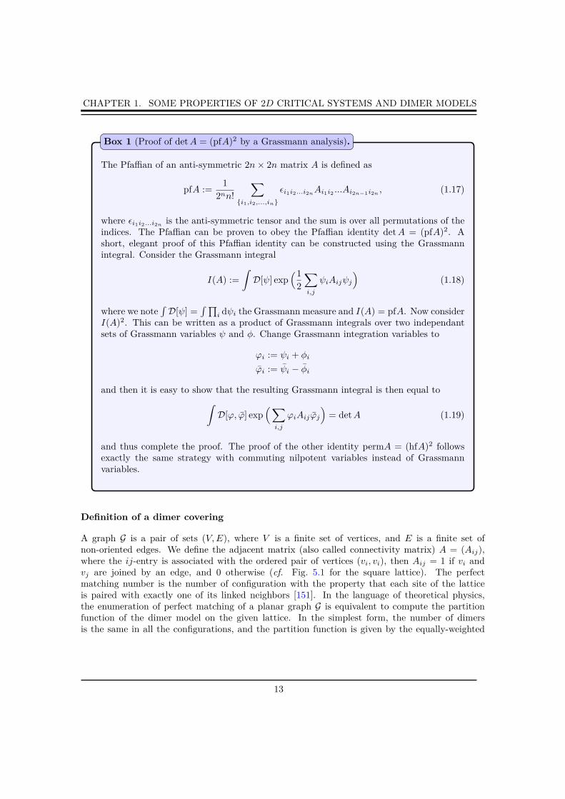
The Pfaffian of an anti-symmetric 2n× 2n matrix A is defined as
pfA :=1
2nn!
∑
{i1,i2,...,in}
ǫi1i2...i2nAi1i2 ...Ai2n−1i2n
, (1.17)
where ǫi1i2...i2nis the anti-symmetric tensor and the sum is over all permutations of the
indices. The Pfaffian can be proven to obey the Pfaffian identity detA = (pfA)2. Ashort, elegant proof of this Pfaffian identity can be constructed using the Grassmannintegral. Consider the Grassmann integral
I(A) :=
∫
D[ψ] exp(1
2
∑
i,j
ψiAijψj
)
(1.18)
where we note∫
D[ψ] =∫∏
i dψi the Grassmann measure and I(A) = pfA. Now considerI(A)2. This can be written as a product of Grassmann integrals over two independantsets of Grassmann variables ψ and φ. Change Grassmann integration variables to
ϕi := ψi + φi
ϕi := ψi − φi
and then it is easy to show that the resulting Grassmann integral is then equal to
∫
D[ϕ, ϕ] exp(
∑
i,j
ϕiAijϕj
)
= detA (1.19)
and thus complete the proof. The proof of the other identity permA = (hfA)2 followsexactly the same strategy with commuting nilpotent variables instead of Grassmannvariables.
Box 1 (Proof of detA = (pfA)2 by a Grassmann analysis).
Definition of a dimer covering
A graph G is a pair of sets (V,E), where V is a finite set of vertices, and E is a finite set ofnon-oriented edges. We define the adjacent matrix (also called connectivity matrix) A = (Aij),where the ij-entry is associated with the ordered pair of vertices (vi, vi), then Aij = 1 if vi andvj are joined by an edge, and 0 otherwise (cf. Fig. 5.1 for the square lattice). The perfectmatching number is the number of configuration with the property that each site of the latticeis paired with exactly one of its linked neighbors [151]. In the language of theoretical physics,the enumeration of perfect matching of a planar graph G is equivalent to compute the partitionfunction of the dimer model on the given lattice. In the simplest form, the number of dimersis the same in all the configurations, and the partition function is given by the equally-weighted
13

CHAPTER 1. SOME PROPERTIES OF 2D CRITICAL SYSTEMS AND DIMER MODELS
(a) (b)
Figure 1.3: (a) Perfect matching of the square lattice, and (b) its ”domino” representation. Thiscombinatorial problem reduces to the calculation of the partition function Eq. (1.20) with t = 1.
average over all possible dimer configurations 3. For example, in the case of the 2 × 2 squarelattice where the weight of dimers are choose to be equal to one, the partition function is just a
sum of two terms= +
. Initially, the dimer model (see Fig. 5.1) has been introducedby physicists to describe absorption of diatomic molecules on a 2d subtrate [78], yet it becamequickly a general problem studied in various scientific communities. From the mathematical pointof view, this problem known as perfect matching problem [151]– is a famous and active problemof combinatorics and graph theory [76] with a large spectrum of applications. The enumeration ofso-called Kekule structures of molecular graphs in quantum chemistry are equivalent to the problemof enumeration of perfect matchings [205, 206]. Besides, a recent connection between dimer modelsand D-brane gauge theories has been discovered [87, 81], providing a very powerful computationaltool.
Haffnian formulation
In the following, we will include equal fugacities t for dimers, so that the average to be taken thenincludes weighting factors for dimers and we write the partition function as
Q0[t] =
∫
D[η] exp(−βH), (1.20)
where the Hamiltonian for the dimer written using commuting nilpotent variables (see Appendix1.1) can be written as a sum over every vertices (see Fig. 1.4), preventing two dimers to occupythe same site
H = − t2
∑
ij
ηiAijηj , (1.21)
where Aij is the adjacent matrix of the lattice considered. Let us put β = 1 in the folllowing. Thenilpotent variables can be seen as commuting Grassmann variables, or simply a product of twosets of standard Grassmann variables where ηi = θiθi. The perfect matching number of the graph
3Throughout this work, we will use the physics terminology and use the expression perfect matching in somespecific cases.
14

CHAPTER 1. SOME PROPERTIES OF 2D CRITICAL SYSTEMS AND DIMER MODELS
η
Figure 1.4: At every vertices, we put a nilpotent variable η, such that η2 = 0 forbidden two dimersto occupy the same site.
G is equal to the partition function in the case t = 1
Q0[1] =
∫
D[η] exp(1
2
∑
ij
ηiAijηj
)
=
∫
D[θ, θ] exp(1
2
∑
ij
θiθiAijθj θj
)
= hfA. (1.22)
In the second line we decomposed the nilpotent variables using two sets of Grassmann variables,and we finally find the well known graph theory result
perfect G = hfA. (1.23)
Considering holes in the perfect matching problem (monomers in the dimer model) is equivalentto remove rows and columns at the positions of the holes in the adjacent matrix (see Fig. 1.5).The resulting combinatorial problem is called the near-perfect matching problem. The partitionfunction of the dimer model with a fixed number of holes (monomers) can be written as
Qn[1] =
∫
D[θ, θ]
n∏
p=1
θqpθqp
exp(1
2
∑
ij
θiθiAijθj θj
)
=
∫
D[θ, θ] exp(1
2
∑
ij
θiθiA\{qp}ij θj θj
)
= hfA\{qp}, (1.24)
where the index n stands for the number of monomers in Qn[t]. Finally, the result is the samebut now the matrix A\{qp} is the adjacent matrix of the original graph with positions of the nmonomers removed. Suppose we remove two sites q1 and q2 on the graph G, then it is similar to
15

CHAPTER 1. SOME PROPERTIES OF 2D CRITICAL SYSTEMS AND DIMER MODELS
n m
(a) (b)
Figure 1.5: (a) Dimer model with 6 monomers, and (b) its ”domino” representation.
introduce two nilpotent variables ηq1 and ηq2 on the lattice, the correlation function between thesetwo monomers is then hfA\(q1,q2)hf−1A and more generally the n-point correlation function reads
⟨
n∏
p=1
ηqp
⟩
=⟨
n∏
p=1
θqpθqp
⟩
=hfA\{qp}
hfA. (1.25)
The partition function and correlations can be studied in the case t 6= 1 as well, in that case,the matrix elements of A are Aij = ±t and the generalization is straightforward. Generallyspeaking, correlations between monomers are equal to correlations between nilpotent variablesin this framework, which can be written in terms of a ratio between two haffnian. Unlike thedeterminant which can be computed by a O(L3) time algorithm by Gauss elimination, there isno polynomial-time algorithm for computing permanent. The problem of converting a permanentproblem into a determinant problem is a long standing problem in pure mathematics, the simplestversion of this problem, is called the Pólya permanent problem [176]. Given a (0, 1)-matrix A :=(Aij)L×L, can we find a matrix B := (Bij)L×L such that permA = detB (or equivalently hfA =pfB) where Bij = ±Aij .
Kasteleyn orientation and Pfaffian formulation
The partition function of the 2d dimer model on the square lattice was solved independentlyusing pfaffian methods [120, 71, 201] for several boundary conditions. Other lattice geometrieshave been studied as well, e.g. the triangular lattice [68], the Kagomé lattice [208, 209, 214], thetriangular Kagomé lattice [149], the hexagonal lattice [66], the star lattice [73], or more complicatedgeometries [215] (see [212] for a review). The Kasteleyn theorem is a recipe to find a matrix4 Kin such way that hfA = pfK, where the elements of the matrix are Kij = ±1. Kasteleyn theoremis based on a special disposition of arrows on the edges of a planar graph5. The product of arrowsaround any even cycle whose interior contains an even (respectively odd) number of vertices is odd(respectively even). Such a disposition is given in Fig. 1.7(b) for the square lattice. We define anantisymmetric matrix K, where Kij = 1 if an arrow points from the site i to the site j, Kij = −1
4We will call this matrix the Kasteleyn matrix in the following.5This is a condicio sine qua non and the theorem is no longer valid for non-planar graph.
16

CHAPTER 1. SOME PROPERTIES OF 2D CRITICAL SYSTEMS AND DIMER MODELS
entat
(a) (b)
Figure 1.6: (a) Square lattice and (b) the orientation prescription of the Kasteleyn matrix.
if the arrow points from j to i, and Kij = 0 otherwise. Let us notice that in general the entriesKij , if they exist, are not necessarily real (see [68] for the triangular lattice). Kasteleyn theoremstates that the perfect matching number of a given planar graph G is given by
perfect G = hfA = pfK, (1.26)
which is equal to ±√
detK. The ± sign is chosen to make the partition function positive, henceforthwe will omit this sign in the rest of the article. Differently, this pfaffian can be express in terms ofGrassmann variables a
pfK =
∫
D[a] exp(1
2
N∑
i,j=1
aiKijaj
)
. (1.27)
Let us mention that this Kasteleyn orientation can be recover with a Grassmann analysis. Thequestion is how to go from the Grassmann haffnian form Eq. (1.22) (with Aij = 1 if the edge i− jand 0 else) to the Grassmann pfaffian form Eq. (1.15) (with Kij unknown). Using straightforwardBerezin manipulations on the haffnian we can check that it is equal to a pfaffian with the properKasteleyn entries Kij . This can be easily generalized for any graph as long as it can be representedwith an adjacent matrix. For the square lattice, we can choose Boltzmann weights tx and tyfor horizontal and vertical dimers, then the pfaffian can be computed by Fourier transform andKasteleyn found for free boundary conditions (cf. [120] for details on calculations)
Q0[tx, ty] =
M/2∏
p=1
N/2∏
q=1
[
4t2x cos2 πp
M + 1+ 4t2y cos2 πq
N + 1
]
. (1.28)
In table 1.1, we compute Q0[1, 1] using Mathematicar, for different M and N with tx = ty = 1
(perfect matching number). All these values can be numerically checked using diverse algorithmswhich enumerate all the possible configurations on the square lattice (see [144] for details). In therest of the paper we will omit the labels tx and ty in the partition function and just keep Q0. Whilethe approach detailed here only works for planar graphs, it is possible to extend beyond that. Forinstance, for any graph that can be embedded on a toroid, the number of dimer distributions canbe expressed as a combination of four pfaffians, as shown by Kasteleyn. The case of surface of highgenius have been studied as well in [53].
17

CHAPTER 1. SOME PROPERTIES OF 2D CRITICAL SYSTEMS AND DIMER MODELS
M \ N 2 4 6 8 10 122 2 5 13 34 89 2334 5 36 281 2245 18061 1456016 13 281 6728 167089 4213133 1069127938 34 2245 167089 12988816 1031151241 8274100582910 89 18061 4213133 1031151241 258584046368 6574373259082112 233 145601 106912793 82741005829 65743732590821 53060477521960000
Table 1.1: Perfect matching number Q0[1, 1] of the square lattice, for different M and N .
Entropy in the thermodynamic limit
The asymptotic form L→∞ of the partition function (for M = N = L) can be easily found fromEq. (5.2)
Q0 ∼ expGL2
π, (1.29)
where is the G is Catalan constant6. The factor G/π is the entropy per site of the dimer modelon the square lattice. This entropy can also be calculated for other bipartite lattices like thehoneycomb lattice, and for non-bipartite lattices like triangular, Kagomé lattice and triangularKagomé lattice. The pfaffian method can be used to compute the partition function of the dimermodel on various geometries and boundary conditions leading to different values of the entropy(cf. [212] for review), as long as the lattice has a Kasteleyn orientation (i.e. planar according tothe Kasteleyn theorem) and as long as N ×M is even. Obviously it is impossible to fill an oddsize lattice with dimers, without leaving one site empty. We shall take notice later that the formof the free energy is strongly dependent of the parity of the lattice.
1.1.3 Local statistics and non-local properties
This theory was used to compute the partition functions, as well as dimer and monomer correlationfunctions in a perturbative way, leading to exact correlation exponents in the thermodynamic limit[71, 72]. In the case of dimer correlations, we will see that, the knowledge of the Kasteleyn matrixis enough to get access to any type of probabilities of configurations while for monomers, things aremuch more complicated and a perturbative modification of the Kasteleyn matrix can be performedto extrapolate the scaling limit of the behavior of monomer correlations.
Dimer correlations
The Kasteleyn matrix is a very powerful objet, which gives us all the details about probabilitiesof presence of dimers [72]. For example the occupation probability of a dimer on the link ij isProba[i→ j] = Kij ×K−1
ij can be computed and we found
6G = 1−2 − 3−2 + 5−2 − 7−2 + ... = 0.915965594...
18
CHAPTER 1. SOME PROPERTIES OF 2D CRITICAL SYSTEMS AND DIMER MODELS
Proba[(x, y)(x+ 1, y)] =4�
(−1)x − (−1)x+1�
(L+ 1)2
L/2�
p,q=1
cos πqL+1 sin2 πpy
L+1
cos2 πpL+1 + cos2 πq
L+1
sinπqx
L+ 1sin
πq(x+ 1)
L+ 1
0 20 40 60 80 100
0.235
0.240
0.245
0.250
0.255
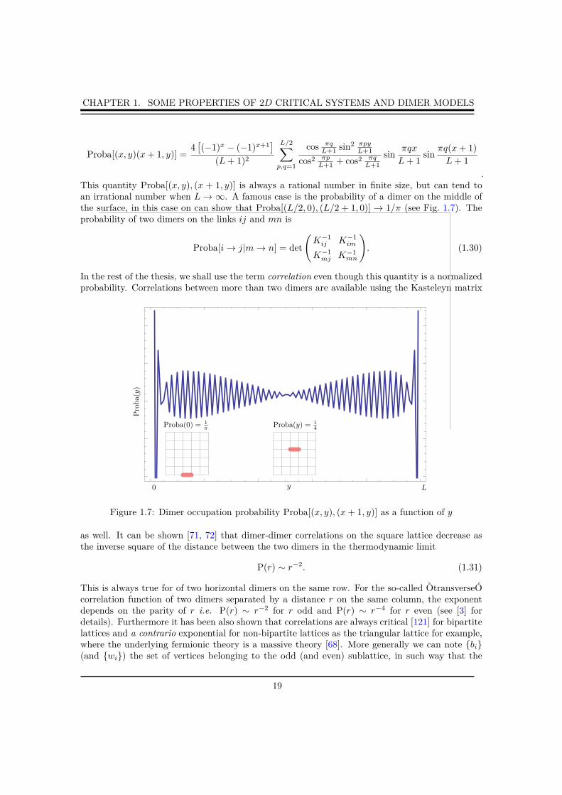
.This quantity Proba[(x, y), (x + 1, y)] is always a rational number in finite size, but can tend toan irrational number when L→∞. A famous case is the probability of a dimer on the middle ofthe surface, in this case on can show that Proba[(L/2, 0), (L/2 + 1, 0)] → 1/π (see Fig. 1.7). Theprobability of two dimers on the links ij and mn is
Proba[i→ j|m→ n] = det
(
K−1ij K−1
im
K−1mj K−1
mn
). (1.30)
In the rest of the thesis, we shall use the term correlation even though this quantity is a normalizedprobability. Correlations between more than two dimers are available using the Kasteleyn matrix
0 20 40 60 80 100
0.235
0.240
0.245
0.250
0.255
Proba(y)
y0 L
Proba(0) = 1π Proba(y) = 1
4
Figure 1.7: Dimer occupation probability Proba[(x, y), (x+ 1, y)] as a function of y
as well. It can be shown [71, 72] that dimer-dimer correlations on the square lattice decrease asthe inverse square of the distance between the two dimers in the thermodynamic limit
P(r) ∼ r−2. (1.31)
This is always true for of two horizontal dimers on the same row. For the so-called ÒtransverseÓcorrelation function of two dimers separated by a distance r on the same column, the exponentdepends on the parity of r i.e. P(r) ∼ r−2 for r odd and P(r) ∼ r−4 for r even (see [3] fordetails). Furthermore it has been also shown that correlations are always critical [121] for bipartitelattices and a contrario exponential for non-bipartite lattices as the triangular lattice for example,where the underlying fermionic theory is a massive theory [68]. More generally we can note {bi}(and {wi}) the set of vertices belonging to the odd (and even) sublattice, in such way that the
19
CHAPTER 1. SOME PROPERTIES OF 2D CRITICAL SYSTEMS AND DIMER MODELS
probability of a configuration of dimer covering Proba[b1 → w1|b2 → w2|b3 → w3|b4 → w4] canbe written in a determinant form. This kind of process is obviously called (by mathematician) adeterminantal process, meaning that any n-point correlation function can be written in terms ofthe determinant of some kernel.
Monomer correlations
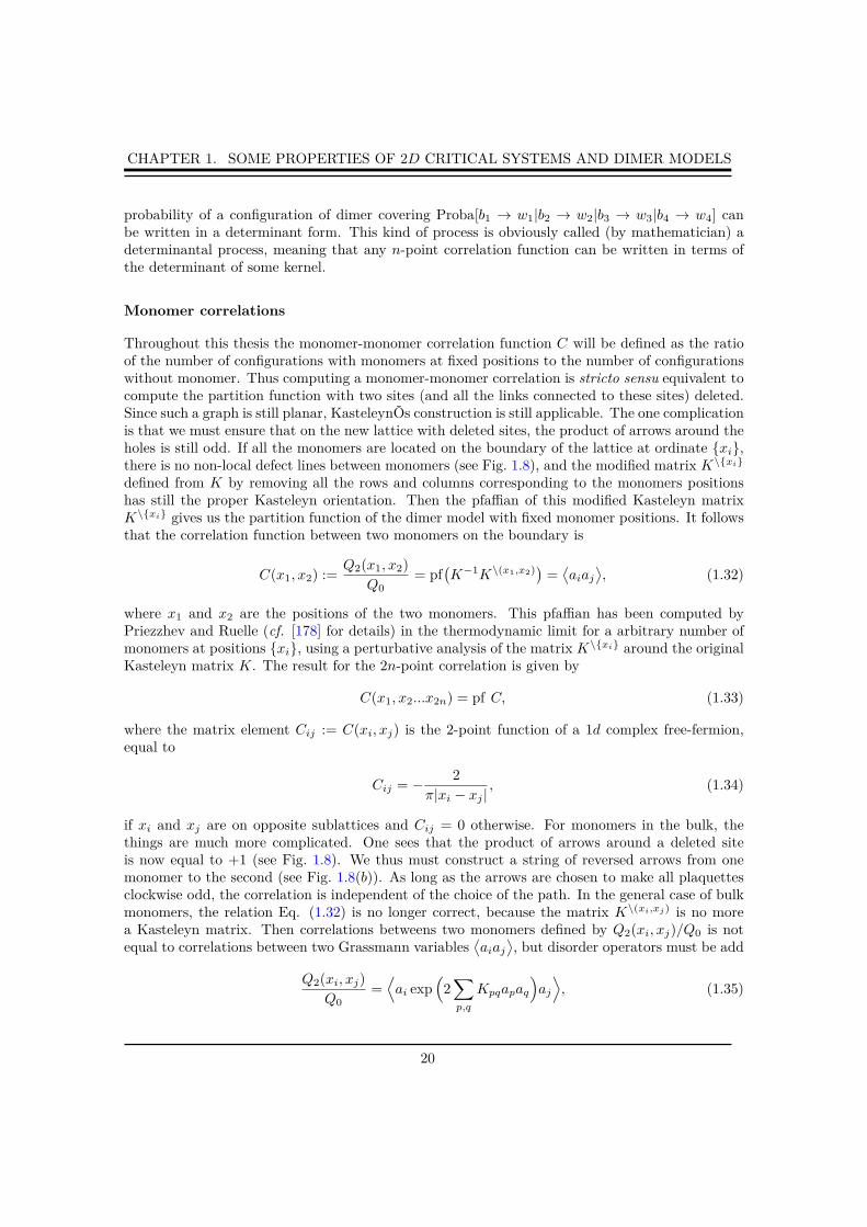
Throughout this thesis the monomer-monomer correlation function C will be defined as the ratioof the number of configurations with monomers at fixed positions to the number of configurationswithout monomer. Thus computing a monomer-monomer correlation is stricto sensu equivalent tocompute the partition function with two sites (and all the links connected to these sites) deleted.Since such a graph is still planar, KasteleynÕs construction is still applicable. The one complicationis that we must ensure that on the new lattice with deleted sites, the product of arrows around theholes is still odd. If all the monomers are located on the boundary of the lattice at ordinate {xi},there is no non-local defect lines between monomers (see Fig. 1.8), and the modified matrix K\{xi}
defined from K by removing all the rows and columns corresponding to the monomers positionshas still the proper Kasteleyn orientation. Then the pfaffian of this modified Kasteleyn matrixK\{xi} gives us the partition function of the dimer model with fixed monomer positions. It followsthat the correlation function between two monomers on the boundary is
C(x1, x2) :=Q2(x1, x2)
Q0= pf
(K−1K\(x1,x2)
)=⟨aiaj
⟩, (1.32)
where x1 and x2 are the positions of the two monomers. This pfaffian has been computed byPriezzhev and Ruelle (cf. [178] for details) in the thermodynamic limit for a arbitrary number ofmonomers at positions {xi}, using a perturbative analysis of the matrix K\{xi} around the originalKasteleyn matrix K. The result for the 2n-point correlation is given by
C(x1, x2...x2n) = pf C, (1.33)
where the matrix element Cij := C(xi, xj) is the 2-point function of a 1d complex free-fermion,equal to
Cij = − 2
π|xi − xj |, (1.34)
if xi and xj are on opposite sublattices and Cij = 0 otherwise. For monomers in the bulk, thethings are much more complicated. One sees that the product of arrows around a deleted siteis now equal to +1 (see Fig. 1.8). We thus must construct a string of reversed arrows from onemonomer to the second (see Fig. 1.8(b)). As long as the arrows are chosen to make all plaquettesclockwise odd, the correlation is independent of the choice of the path. In the general case of bulkmonomers, the relation Eq. (1.32) is no longer correct, because the matrix K\(xi,xj) is no morea Kasteleyn matrix. Then correlations betweens two monomers defined by Q2(xi, xj)/Q0 is notequal to correlations between two Grassmann variables
⟨aiaj
⟩, but disorder operators must be add
Q2(xi, xj)
Q0=⟨ai exp
(2∑
p,q
Kpqapaq
)aj
⟩, (1.35)
20

CHAPTER 1. SOME PROPERTIES OF 2D CRITICAL SYSTEMS AND DIMER MODELS
(a) (b)
10 5020 3015
104
0.001
0.005
0.010
0.050
60. 65. 70.
0.028
0.029
0.03
0.031
0.032
0.033
0.034
0.035
Figure 1.8: Modification of the Kasteleyn matrix in the presence of two monomers. The monomers(red dots) destroy the corresponding links and the orientation (a) has to be changed to respect theproper orientation (b).
where the sum is over all the links connecting sites i and j, to take account of the reversing linebetween the two monomers. Using a pfaffian perturbative analysis it was shown that monomercorrelations decrease at the thermodynamic limit as [71, 72]
C(r) ∼ r−1/2. (1.36)
This result is very similar to the construction of the spin correlation functions in the Ising modelin terms of fermionic variables [118, 177]. In fact, on the square lattice, the monomer-monomercorrelations was shown to have the same long-distance behavior as the spin-spin correlations intwo decoupled Ising models, explained by the deep relation between the two correlation functionsfor the square lattice given by Perk and Au-Yang [13]. These disorder operators are absent in thehaffnian theory Eq. (1.25), and are the price to pay to solve the problem analytically.
1.2 Relation to other statistical models
The prominence of the dimer model in theoretical physics and combinatorics also comes from thedirect mapping between the square lattice Ising model without magnetic field and the dimer modelon a decorated lattice [154, 120, 71, 201] and conversely from the mapping of the square latticedimer model to a eight-vertex model [16, 211]. Furthermore the magnetic field Ising model can bemapped onto the general monomer-dimer model [90].
1.2.1 Back to Ising
The formulation of the Ising model in term of graph-expansion (as we saw in the beginning ofthe chapter) can be related to dimer configurations on a decorated square lattice [121] (as shownFig. 1.9). Every graph of the partition function of the Ising model can be written using thismapping, but the mapping is not so explicit because of several serious issues.
• Since a vertex with no polygons corresponds to three dimer configurations on the internal
21

CHAPTER 1. SOME PROPERTIES OF 2D CRITICAL SYSTEMS AND DIMER MODELS
Figure 1.9: Left: a graph of order b4 in the high temperature expansion of the Ising model on thesquare lattice and (center) its corresponding dimer covering in a decorated Fisher lattice. Right:Kasteleyn orientation of the decorated graph.
decoration(
) =(
), the mapping is not "one-to-one" but "one-to-three".
• Second, the decorated lattice is a non-planar graph and as we saw earlier, the Kasteleyntheorem breaks down in that case, and it is not obvious that a proper Kasteleyn orientationdoes exist.
Actually, if one considers the orientation of the decorated lattice shown in Fig. 1.9, one can verifythat the oriented graph is actually properly Kasteleyn oriented and that the pfaffian of this matrixis the perfect matching of the lattice. This seems to be a coincidence since the two complicationscancel each other exactly (see [121] for details).
1.2.2 Temperley bijection and spanning trees
Another problem which is of great interest in lattice statistical physics is the computation of thenumber of spanning trees covering a given graph G. The resolution of this problem comes to theuse of another ”graph-theory” matrix know as the Laplacian matrix. This problem is describedby a free fermionic field theory via the matrix-tree theorem, stating that the number of spanningtrees on a graph G is given by the determinant of a minor of the Laplacian matrix ∆ of G (cf.[155]). Using that, the partition function of spanning trees on the square lattice can be computedand the result looks very similar to the dimer model. Indeed, Temperley [200] found a bijectionbetween spanning trees on the m× n square lattice and dimer covering of the (2m+ 1) × (2n+ 1)square lattice with a boundary site removed.
• The mapping is a bijection, to each configuration of dimer on the (2m+ 1) × (2n+ 1) latticecorresponds to a unique spanning tree on the 2m× 2n.
• The position of the monomer does not matter, as long as it is on the boundary and on theproper sublattice7. This observation tells us that the partition function of dimer with one
7To convince ourselves we need at least a 5 × 5 lattice, because on the 3 × 3 lattice shown Fig. 1.2.2, the onlypossibility is to put the monomer on one of the four corners.
22
CHAPTER 1. SOME PROPERTIES OF 2D CRITICAL SYSTEMS AND DIMER MODELS
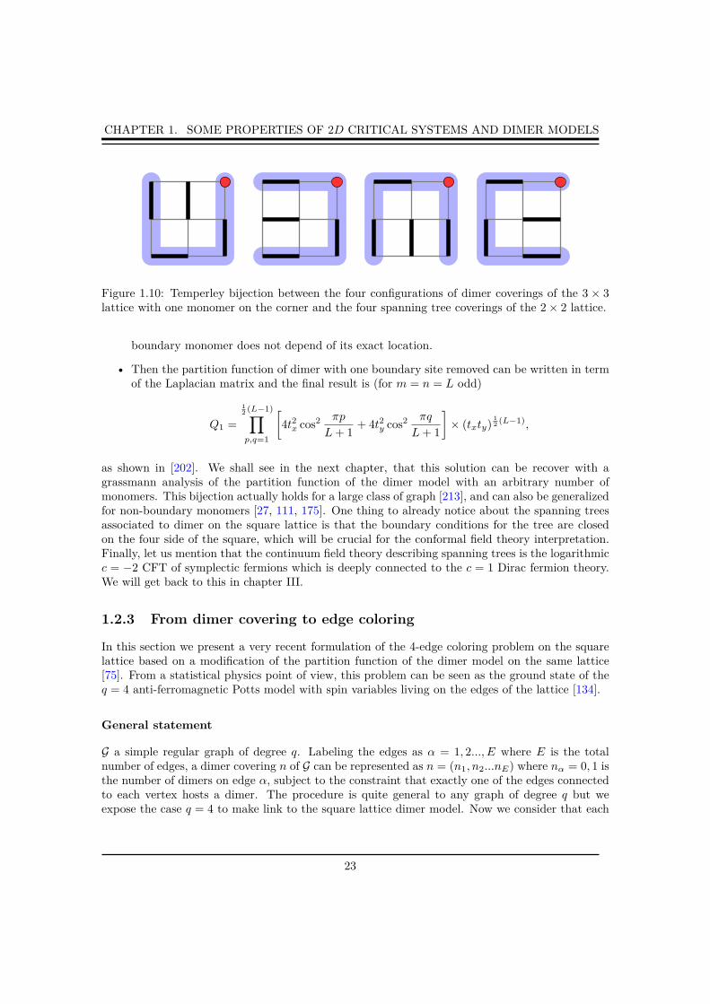
Figure 1.10: Temperley bijection between the four configurations of dimer coverings of the 3 × 3lattice with one monomer on the corner and the four spanning tree coverings of the 2 × 2 lattice.
boundary monomer does not depend of its exact location.
• Then the partition function of dimer with one boundary site removed can be written in termof the Laplacian matrix and the final result is (for m = n = L odd)
Q1 =
12 (L−1)∏
p,q=1
[4t2x cos2 πp
L+ 1+ 4t2y cos2 πq
L+ 1
]× (txty)
12 (L−1),
as shown in [202]. We shall see in the next chapter, that this solution can be recover with agrassmann analysis of the partition function of the dimer model with an arbitrary number ofmonomers. This bijection actually holds for a large class of graph [213], and can also be generalizedfor non-boundary monomers [27, 111, 175]. One thing to already notice about the spanning treesassociated to dimer on the square lattice is that the boundary conditions for the tree are closedon the four side of the square, which will be crucial for the conformal field theory interpretation.Finally, let us mention that the continuum field theory describing spanning trees is the logarithmicc = −2 CFT of symplectic fermions which is deeply connected to the c = 1 Dirac fermion theory.We will get back to this in chapter III.
1.2.3 From dimer covering to edge coloring
In this section we present a very recent formulation of the 4-edge coloring problem on the squarelattice based on a modification of the partition function of the dimer model on the same lattice[75]. From a statistical physics point of view, this problem can be seen as the ground state of theq = 4 anti-ferromagnetic Potts model with spin variables living on the edges of the lattice [134].
General statement
G a simple regular graph of degree q. Labeling the edges as α = 1, 2..., E where E is the totalnumber of edges, a dimer covering n of G can be represented as n = (n1, n2...nE) where nα = 0, 1 isthe number of dimers on edge α, subject to the constraint that exactly one of the edges connectedto each vertex hosts a dimer. The procedure is quite general to any graph of degree q but weexpose the case q = 4 to make link to the square lattice dimer model. Now we consider that each
23

CHAPTER 1. SOME PROPERTIES OF 2D CRITICAL SYSTEMS AND DIMER MODELS
edge α has a Boltzmann weight wα and we formally write the the dimer partition function as
Q0 =∑
n
∏
α
wnαα . (1.37)
Next, we introduce colored dimers and define a 4-colored dimer covering which consists of dimers
g = 0 g = 1
Figure 1.11: The four coloring problem seen as interacting layers of dimers. On the left one havefour independent dimer coverings (g = 0) and on the right the 4-egde coloring problem (g = 1)
that all have the same color, which may take one out of 4 values: µ = 1, 2, 3, 4. Because allvertices have degree 4, any 4-edge-coloring of G is also a 4-dimer-covering, but unlike generic 4-dimer-coverings it satisfies the additional Òcoloring constraintÓ that no edge should have morethan one dimer. We therefore want to extract the former from the latter. To this end, considerthe partition function for 4-dimer-coverings, i.e four independent layers of colored dimer covering,which is given by
Q40 =
∑
n(1)...n(4)
∏
α
wn(1)
α +n(2)α +n(3)
α +n(4)α
α , (1.38)
where nµ denotes a µ-colored dimer covering of the lattice. This corresponds to the point g = 0 inFig. 1.11. Each term in the sum corresponds to a 4-dimer-covering. A term that also correspondsto a 4-edge-coloring will contain exactly one factor of wα for each edge α. Conversely, for a termthat does not correspond to a 4-edge-coloring, at least one edge α will contain more than one dimerand thus comes with a factor wpα with p > 2, and, equivalently, at least one edge β will not havea dimer and thus comes with a factor w0
β = 1. The latter property implies that if we successively
= w1w22w3w
04
= w1w2w3w4
differentiate a term in the last equation with respect to each dimer weight wγ , the final result willbe 1 for any term representing a 4-edge-coloring and 0 for all other terms, which corresponds tothe point g = 1 in Fig. 1.11. Therefore the number of 4-edge-colorings Zcolor is given by
Zcolor =(∏
α
∂wα
)Q4
0. (1.39)
We have thus shown that the number of 4-edge-coloring Z can be obtained from the partitionfunction Q0 of the dimer model with edge-dependent dimer weights w on the same graph. This
24

CHAPTER 1. SOME PROPERTIES OF 2D CRITICAL SYSTEMS AND DIMER MODELS
formulation of the generating function of the coloring problem in terms of dimer coverings holdsfor any regular graph G.
Grassmann formulation
Now we can express the partition function of the dimer model using Grassmann variables as wedid before, we have now to introduce 4 types of colored Grassmann variables a(µ)
Q40 =
∫ 4∏
µ=1
D[a(µ)] exp(1
2
∑
µ
N∑
i,j=1
a(µ)i Kija
(µ)j
), (1.40)
where the µ stands for the four differents set of Grassmann variables and where the Kasteleynmatrix Kij stands here for wijKij . Here we do not expose the demonstration in great details andwe send the reader back to the original paper [75]. By adding a pair of Grassmann variables ξij andξij for each link Kij , we ensure that it can be used only by one of the color for each distribution, ifit was used by two or more we would get at least a double instance of that Grassmann variable, andhence get 0. However, as we are dealing with Grassmann variables, this leads to sign problems. Wecan avoid that by observing that a pair of Grassmann variables always commutes, and thus doesnot give us any additional sign trouble. Thus we now have the following formula for the numberof 4-coloring of the square lattice
Zcolor =
∫ 4∏
µ=1
D[a(µ)] exp(1
2
∑
µ
N∑
i,j=1
a(µ)i ξijKijξija
(µ)j
). (1.41)
We end up with a quartic fermionic which is of course non-solvable by pfaffian methods. Anotherapproach based on a height mapping can also be followed, leading to several theoretical predictionsabout the critical behavior of this model and support the conjecture that the scaling limit8 iswell described by a Wess-Zumino-Witten SU(4)k=1 conformal field theory [134]9. This particularproblem can be shown to be a special point in the parameter space of compact polymers modelcalled FPL2 [110, 108].
1.3 About the full monomer-dimer model
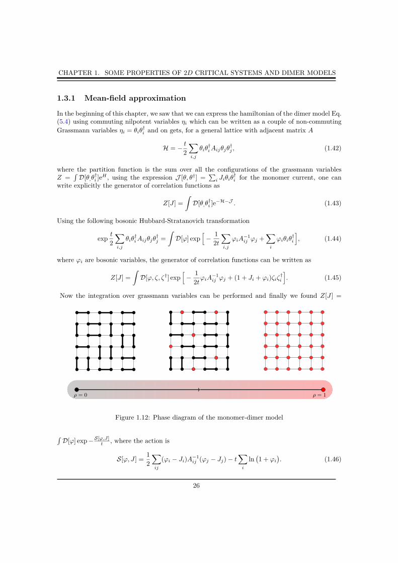
The general monomer-dimer problem is a much more complex and challenging problem in statisticalphysics and combinatorics, it is defined as the dimer model with a finite density of monomers(see Fig. 1.12). The challenge is to compute the partition function for any density. For thegeneral monomer-dimer problem there is no exact solution except in 1d, on the complete andlocally tree-like graphs [2] or scale free networks [216]. Furthermore the behavior of monomer-monomer correlations for finite density has been studied numerically [145], and strong evidencesfor exponential correlations has been established, in accordance with mean-field calculations usingGrassmann variables [167]. From a computational point of view, this lack of exact solution hasbeen formalized [112] and the problem has been shown to belong to the #P -complete enumerationclass [112].
8The two points g = 0 and g = 1 of Fig. 1.11 seem to be very well understood but we can ask ourselves whatabout in between ?
9Which was apparently conjectured by N.Read in a private communication
25
CHAPTER 1. SOME PROPERTIES OF 2D CRITICAL SYSTEMS AND DIMER MODELS
1.3.1 Mean-field approximation
In the beginning of this chapter, we saw that we can express the hamiltonian of the dimer model Eq.(5.4) using commuting nilpotent variables ηi which can be written as a couple of non-commuting
Grassmann variables ηi = θiθ†i and on gets, for a general lattice with adjacent matrix A
H = − t
2
∑
i,j
θiθ†iAijθjθ
†j , (1.42)
where the partition function is the sum over all the configurations of the grassmann variablesZ =
∫D[θ,θ
†i ]e
H , using the expression J [θ, θ†] =∑i Jiθiθ
†i for the monomer current, one can
write explicitly the generator of correlation functions as
Z[J ] =
∫D[θ,θ
†i ]e
−H−J . (1.43)
Using the following bosonic Hubbard-Stratanovich transformation
expt
2
∑
i,j
θiθ†iAijθjθ
†j =
∫D[ϕ] exp
[− 1
2t
∑
i,j
ϕiA−1ij ϕj +
∑
i
ϕiθiθ†i
], (1.44)
where ϕi are bosonic variables, the generator of correlation functions can be written as
Z[J ] =
∫D[ϕ, ζ, ζ†] exp
[− 1
2tϕiA
−1ij ϕj + (1 + Ji + ϕi)ζiζ
†i
]. (1.45)
Now the integration over grassmann variables can be performed and finally we found Z[J ] =
ρ = 0 ρ = 1
Figure 1.12: Phase diagram of the monomer-dimer model
∫D[ϕ] exp − S[ϕ,J]
t , where the action is
S[ϕ, J ] =1
2
∑
ij
(ϕi − Ji)A−1ij (ϕj − Jj) − t
∑
i
ln(1 + ϕi
). (1.46)
26

CHAPTER 1. SOME PROPERTIES OF 2D CRITICAL SYSTEMS AND DIMER MODELS
In order to extract information about this system, we shall use a saddle point approximation
Z[J ] =
∫D[ϕ] exp
[− S[ϕ, J ]
t
]= exp
[− S[ϕ, J ]
t
](1 + O(t)
), (1.47)
where ϕ is solutions of δS/δϕi = 0.
δSδϕi
= 0→ ρi =1
t
∑
j
A−1ij ϕj =
1
1 + ϕi, (1.48)
hence
Ji = ρ−1i − 1− t
∑
j
Aijρj . (1.49)
and the correlation function is
Cki =∂ρk∂Ji
=(− tAki −
δkiρ2k
)−1
. (1.50)
Now we can write the effective action in the saddle point approximation by using the aboveexpression of ρk in function of the field in the saddle point ϕk, and we get
S[J ] =1
2
∑
ij
ρiAijρj +∑
i
ln ρi. (1.51)
Using this effective action in presence of a current of monomers, we can use standard field theorymethods to compute the density ρi = 〈θiθ†
i 〉, and correlation function of monomers like 〈ρiρj〉 =
〈θiθ†i θjθ
†j〉 or more complicated object using functional derivatives of the generator of correlation
functions Z[J ]
〈ρi1 ...ρiN 〉 = limJ→0
1
Z[0]
δNZ[J ]
δJi1 ...δJiN. (1.52)
If we want to look at connected correlation functions, we shall introduce W[J ] = lnZ[J ] such that
δW[J ]
δJi=∑
kl
[ρ0 − 1
ρ2k
δkl + pAkl(ρ0 − ρk)] δρlδJi
+ ρ0 = ρi.
Correlation functions can be obtained by taking derivatives as follow
Cij = 〈ρiρj〉c = limj→0
δ2W[J ]
δJiδJj=∂ρi∂Jk
.
The effective action is then
Γ[ρ] =W[J ] +∑
i
Jiρi (1.53)
= − p
2
∑
ij
ρiAijρj +∑
i
ln ρi +∑
i
(1− ρi).
27

CHAPTER 1. SOME PROPERTIES OF 2D CRITICAL SYSTEMS AND DIMER MODELS
We specialize now to the case of uniform hole density ρi = ρ and also for the case of the squarelattice where the number of nearest neighbors is four and assuming that the number of sites onthe lattice is N . Then,
Γ[ρ] =−4zNρ2
2+N logN +N(1 − ρ), (1.54)
and the current can be written as J = −4tρ+ ρ−1 − 1, sending the current to zero give the densityin terms of t
ρ =2
1 +√
1 + 16t. (1.55)
So in the region t → 0, t = 1 − 4ρ. Now we compute the propagator Cij , δij become A(q) =2a∑k=x,y cos qka, such that
C(q) =(ρ−2 − 2ta
∑
k=x,y
cos qka)−1
. (1.56)
The conclusion of this mean-field calculation is that for any non-zero monomer density, the systemis non-critical (with a finite correlation length). This mean-field analysis gives a rather goodapproximation of the behavior of the system, but more involved technics have to be implementedto get access to non mean-field results, as the exact value of the correlation length.
1.3.2 Baxter approach and matrix product state
One cannot conclude this chapter on the monomer-dimer model without mentioning one of themost impressive advance, which the numerical solution of the model by Baxter [15], with a methodwhich is sometimes referred as variational transfer matrix approach, but which is nothing but thematrix product state method that we know today. This method is very efficient to compute preciseapproximations of thermodynamic quantities of the model.
Figure 1.13: Vertex representation of the monomer-dimer model. The extreme-right vertex corre-sponds to a monomer with weight 1, and the others correspond to vertical and horizontal dimerswith weights s2
Transfert matrix formulation
Let us consider a square lattice of size m × n with periodic boundary conditions. For any site(i, j), the occupation of horizontal edges is given by the binary variables βi,j and βi+1,j and the
28

CHAPTER 1. SOME PROPERTIES OF 2D CRITICAL SYSTEMS AND DIMER MODELS
occupation of vertical edges is given by αi,j and αi,j+1 such that a vertex has a Boltzmann weightω(αi,j , αi,j+1|βi,j , βi+1,j) which is equal to zero when there is more than one dimer on every vertex,i.e. αi,j + αi,j+1 + βi,j + βi+1,j > 1. Then the partition function can be written as
Z =∑
{α,β}
∏
(i,j)
ω(αi,j , αi,j+1|βi,j , βi+1,j). (1.57)
This expression is the usual form of the partition function of a vertex model with vertex weight ω.In this fashion the monomer-dimer model is mapped onto a 5-vertex model as show on Fig. 1.14.The partition function can be written in another form
Z =∑
{β}
m∏
i=1
T (βi+1,1, ..., βi+1,n|βi,1, ..., βi,n)︷ ︸︸ ︷(∑
{α}
n∏
j=1
ω(αi,j , αi,j+1|βi,j , βi+1,j)), (1.58)
in such way that the partition function reduces to a trace over the vectorial space V ⊗ V ∗10
Z =∑
{β}
m∏
i=1
T (βi+1,1, ..., βi+1,n|βi,1, ..., βi,n)
=∑
β1,1...β1,n,βm,1...βm,n
T (β1,1, ...|βm,1, ...)...T (β3,1, ...|β2,1, ...)...T (β2,1, ...|β1,1, ...)
= Tr Tm, (1.59)
where T is the vertical transfer matrix with matrix element T (βi+1,1, ..., βi+1,n|βi,1, ..., βi,n). Asusual, in the limit m→∞, the trace is dominated by the largest eigenvalue Λ of T and
Z ∼ Λm. (1.60)
Product matrix state formulation
Let us define |Λ〉 the eigenvector corresponding to the largest eigenvalue Λ of the transfer matrixT . For any vector |ψ0〉 ∈ V , we have
Tm|ψ0〉 ∼ Tm|Λ〉〈Λ|ψ0〉. (1.61)
Now let us choose 〈β1, β2, ..., βn|T |ψ0〉 = 1 such that
〈β′1, β
′2, ..., β
′n|T |ψ0〉 =
∑
β1,...,βn
T (β′1, β
′2, ..., β
′n|β1, β2, ..., βn)〈β1, β2, ..., βn|ψ0〉, (1.62)
=∑
β1,...,βn
∑
α1,...,αn
n∏
j=1
ω(αj , αj+1|βj , β′j+1). (1.63)
10V = Z⊗n2
29

CHAPTER 1. SOME PROPERTIES OF 2D CRITICAL SYSTEMS AND DIMER MODELS
The same calculation can be repeated for Tm, after a few lines of calculation we end up with
〈βm+1,1, ..., βm+1,n|Tm|ψ0〉 =∑
α1,1,...,α1,n
n∏
j=1
∑
β1,j ,...,βm,j
m∏
i=1
ω(αi,j , αi,j+1|βi,j , βi+1,j). (1.64)
The transfer matrix T correspond to the partition function of a system with a single columnwith weights αi,j (j = 1...n) and fixed horizontal weights βij and βi+1,j . This partition functionIt is convenient to attribute the Boltzmann weight for each Vertex.
There are 5 vertex configurations:
Vertex Weight K:
K = 1 for empty vertex.
K = s
K = t
We denote horizontal bond variable (= 0 or 1) by ‘ ’ and vertical one by ‘b’.
a a’
b
b’
Partition Function of the system can be represented as a configuration sum for the product of local Boltzman weights.
0 1 2 3 4 5
1
2
3
4
5
6
1/s
Z/s
Figure 1.14: Left: Vertex representation of the monomer-dimer model. Partition Function of thesystem can be represented as a sum of product of local Boltzmann weights. Right: Numericalresults from Baxter’s method. The partition function increases smoothly with s−1 indicating nophase transition in this model. The point s−1 = 0 is the exact solution saw in the beginning of thechapter and equal to exp(G/π) ≈ 1.338.., with G is the Catalan constant.
can computed introducing another transfer matrix for which βij and βi+1,j are parameters. Theelements of this transfer matrix are
Gβm+1,j(α′
1, ..., α′n|α1, ..., αn) = 〈α′
1...α′n|Gm+1,j |α1...αn〉
=∑
β1,j ,...,βm,j
m∏
i=1
ω(αi,j , αi,j+1|βi,j , βi+1,j), (1.65)
such that
〈βm+1,1, ..., βm+1,n|Tm|ψ0〉 =∑
α1,1...α1,n,αm,1...αm,n
n∏
j=1
Gβm+1,j(α1,j+1, ..., αn,j+1|α1,j , ..., αn,j)
= TrH
[Gm+1,nGm+1,n−1...Gm+1,1
], (1.66)
where we choose periodic boundary conditions αm+1,j = α1,j and H = Z⊗m2 is a vectorial space
encoding the configurations of links α on a row. Finally
|Λ〉 ∼ 〈βm+1,1, ..., βm+1,n|Tm|ψ0〉 = TrH
[Gm+1,nGm+1,n−1...Gm+1,1
], (1.67)
30

CHAPTER 1. SOME PROPERTIES OF 2D CRITICAL SYSTEMS AND DIMER MODELS
we have expressed the vector |Λ〉 as a matrix product state, and starting from the expression Eq.(1.67), the next will be to use a variational principle to optimize the matrices G, some details canbe found in the original paper [15], and we show on figure 1.14 numerical results of this method11.It is quite clear that the numerical calculations do not show any divergences of the thermodynamicquantities then no phase transition for any non-zero densities. This numerical method can beapplied to any model with local Boltzmann weights defined on the vertices of a lattice and futurechallenge emerging out of this present work is the study of other two dimensional dimer relatedmodels as the trimer model [83] or the four-color model [134, 75] which can be seen as an interactingcolored dimer model.
1.3.3 Heilmann-Lieb theorem and Ising model in a magnetic field
From a computational point of view, the problem has been shown to belong to the #P -completeenumeration class [112] and all the methods available are either efficient but approximative [15, 125]or exact but desperately slow [1]. Let us start by counting the number of ways N2p(M,N) ofchoosing the positions of 2p monomers on a M×N lattice, the result is a simple binomial expression
N2p(M,N) =(M2/2p
)(N2/2p
). Using this formula we can sum up over the number of monomers 2p
to obtain the number of ways to choose the positions of the monomers. Finally the number ofterms in the full partition function is one (the pure dimer model) plus all the terms with an evennumber of monomers (one choose M = N = L for simplicity)
N(L) = 1 +
L2/2∑
p=1
N2p(L) =2L
2
Γ(L2+1
2
)√πΓ(L2+2
2
) . (1.68)
This number grows as 2L2
when the size of the lattice goes to infinity, making the problem impos-sible to solve analytically. We can formally write down the full monomer-dimer partition functionas a sum over the number and the positions of monomers
ZM×N = Q0 +∑
{ri}
Q2 +∑
{ri}
Q4 + ...+∑
{ri}
QM×N , (1.69)
where Q0 is the dimer partition function, and Q2, Q4...QM×N are the partition functions with two,four...M×N monomers with fixed positions. For concreteness12, we consider the partition function
= + + + + + +
Figure 1.15: Diagrammatic representation of Eq. (1.69), the first two diagrams are Q0, the fournext are Q2 and the last is Q4. The coefficient here are different Z2×2(x) = x4 + 4x2 + 2, becausethe condition are free on the figure and periodic in Eq. (1.69).
11Thanks to Christophe Chatelain for the simulations and for discussions on this problem12The presentation and the enumerative results come again from the book of W.Krauth [144].
31

CHAPTER 1. SOME PROPERTIES OF 2D CRITICAL SYSTEMS AND DIMER MODELS
ZL×L(β) for an L×L square lattice with periodic boundary conditions and we follow closely [144].ZL×L(β) is a polynomial in x = e−βǫ with positive coefficients which, for small lattices, are givenby
Z2×2(x) = x4 + 8x2 + 8, (1.70)
Z4×4(x) = x16 + 32x14 + 400x12 + ...+ 3712x2 + 272,
Z6×6(x) = x36 + 72x34 + ...+ 5409088488x12 + ...+ 90176.
The coefficients of Z2×2(x) correspond to the fact that in the 2×2 lattice without periodic boundaryconditions, we can build one configuration with zero dimers and eight configurations each with oneand with two dimers (see Fig. 1.3.3). Generally for a L× L lattice
ZL×L =
L2/2∑
k=0
α2kx2k, (1.71)
where the αk are the number of configurations of dimers with k monomers. The way a phasetransition can nevertheless take place in the limit of an infinite system limit involves consideringthe partition function as a function of x, taken as a complex variable, and study the repartition ofthe positions of the zeros on the complex plane. For the monomer-dimer model, Heilmann and Lieb
Standard algorithms allow us to compute the (complex-valued) zeros of these polynomi-als, that is, the values of x for which ZL×L(x) = 0, etc. For all three lattices, the zerosremain on the imaginary axis, and the partition function can be written as
Z2×2(x) = (x2 + 1.1716)(x2 + 6.828), (1.72)
Z4×4(x) = (x2 + 0.102)(x2 + 0.506)...(x2 + 10.343),
Z6×6(x) = (x2 + 0.024)(x2 + 0.121)...(x2 + 10.901).
Generally we can write the partition function as a product
ZL×L =
L2∏
k=1
(x+ izk), (1.73)
where {zk} are the zeros of the function ZL×L. It is shown that, for given non-negativeweight , ZL×L cannot be zero if !(xi) > 0 ∀i = 1, 2...L×L or if !(xi) < 0 ∀i = 1, 2...L×L.In particular, if xi ∀i = 1, 2...L× L , this leads to the conclusion that the zeros of ZL×L
appear on the imaginary-x axis (or at x = 0), a result that holds also in the appropriatethermodynamic limit. Now in order to complete the proof, one must show that the zerosstay on the imaginary axis and never cross the real one at the thermodynamic limit.More generally, it can be showed by recursion that the zeros of the partition functionfor any lattice are sandwiched in by the zeros of partition functions for lattices with onemore site (see [125] for details), concluding the proof of absence of phase transition inany dimensions and for any lattices.
Box 2 (Sketch of the proof).
32

CHAPTER 1. SOME PROPERTIES OF 2D CRITICAL SYSTEMS AND DIMER MODELS
shown in a famous work [89, 90] that the zeros stay on the imaginary axis. This corresponds to theabsence of a phase transition in the monomer-dimer system in any dimension, except, eventually,at x = 0 which correspond to the pure dimer case, confirming the results of Baxter presented inthe past section. A partial proof of this result is shown in the box 2 above. A natural extensionof this model, is to add interactions between dimers on the same plaquette for instance. It hasbeen shown that for a range of values of the interaction, the system can be critical even with anon-zero monomer density [4, 3, 167]. A short introduction of this model will be discussed in theend of the third chapter.
1.4 Conclusions
In this chapter, we gave a rather personal overview of the field of combinatorial statistical modelsand specially systems which are related to dimer models. We have voluntary chosen very fewsimple examples that are relevant for this study and omit a lot of technicalities. In particular wehave mentioned a couples of times relations to conformal field theory that we have not defined inmuch details, for sake of clarity. Nevertheless, in the third chapter of this thesis, a more detailedcomparison to conformal field theory will be examined, and some of the most familiar applicationswill be treated. We have seen that non-commuting variables are very useful to describe the partitionfunction of this kind of models. In the next chapter, this approach will used in a rather differentway to compute exactly the partition function of the simple dimer model. We shall focus in thecomputation of the extension of the dimer model when one allows for the presence of a finitenumber of fixed monomers. While this problem is very difficult to handle with the Kasteleyntheory, leading only to results in a perturbative way, the alternative approach will give us theexact expression on a discrete level.
33

CHAPTER 2. DIMER MODEL: PLECHKO SOLUTION AND GENERALIZATION
CHAPTER2Dimer model: Plechko solution and generalization
Contents
2.1 Plechko solution . . . . . . . . . . . . . . . . . . . . . . . . . . . . . . . 35
2.1.1 Fermionization and mirror symmetry . . . . . . . . . . . . . . . . . . . . 35
2.1.2 Pfaffian solution without monomer . . . . . . . . . . . . . . . . . . . . . 36
2.1.3 Majorana fermions lattice theory . . . . . . . . . . . . . . . . . . . . . . 39
2.2 Pfaffian solution with 2n monomers . . . . . . . . . . . . . . . . . . . 41
2.2.1 General solution of the problem . . . . . . . . . . . . . . . . . . . . . . . 42
2.2.2 Boundary monomers and 1d complex fermion chain . . . . . . . . . . . 48
2.2.3 Single monomer on the boundary and localization phenomena . . . . . . 52
2.3 Fun with dimers . . . . . . . . . . . . . . . . . . . . . . . . . . . . . . . 54
2.3.1 Partition function without monomers . . . . . . . . . . . . . . . . . . . 54
2.3.2 Partition function with two boundary monomers . . . . . . . . . . . . . 55
2.3.3 Partition function with 2n boundary monomers . . . . . . . . . . . . . . 57
2.4 Conclusions of the chapter . . . . . . . . . . . . . . . . . . . . . . . . . 58
34
CHAPTER 2. DIMER MODEL: PLECHKO SOLUTION AND GENERALIZATION
In this chapter, the fully-detailed Grassmann solution of the dimer model originally foundby Plechko is presented, as well as informations you can get for the Ising model. Then the solutionis extended for the case with an arbitrary number of monomers, which will lead to the exact formof correlation functions in a pfaffian formulation. In particular, we show that the problem becomesimpler when we consider boundary monomers, and a closed expression for correlations can befound. After that, the simple application of the case of one boundary monomer is shown to beexactly the known result confirming the exactness of our solution. We shall finish by noticing somepurely combinatorial properties of the partition function with boundary monomers.
2.1 Plechko solution
The approach introduce presently has been developed by Plechko in a series of papers [171, 172]and allows for the exact partition function for the 2d Ising model. In this chapter we briefly recallthe method of resolution of the 2d dimer model based on the integration over Grassmann variablesand factorization principles for the partition function. The hamiltonian of the dimer model on ageneral graph can be written as we saw before as
Q0 =
∫D[η] exp
(− t
2
∑
ij
ηiAijηj
), (2.1)
which in the particular case of a square lattice of size L× L with L even takes the following form
Q0 =
∫D[η]
L∏
m,n
(1 + txηmnηm+1n)(1 + tyηmnηmn+1), (2.2)
where ηmn are nilpotent and commuting variables on every vertices of the square lattice.
2.1.1 Fermionization and mirror symmetry
The integrals can be computed introducing a set of Grassmann variables (amn, amn, bmn, bmn), (cf.Fig. 2.1(a)), such that
(1 + txηmnηm+1n) =
∫D[a] D[a]eamnamn(1 + amnηmn)(1 + txamnηm+1n),
(1 + tyηmnηmn+1) =
∫D[b] D[b]ebmnbmn(1 + bmnηmn)(1 + ty bmnηmn+1). (2.3)
This decomposition allows for an integration over variables ηmn, after rearranging the differentlink variables Amn := 1 +amnηmn, Am+1n := 1 + txamnηm+1n, Bmn := 1 + bmnηmn and Bmn+1 :=1 + ty bmnηmn+1. Then the partition function becomes
Q0 = Tr{a,a,b,b,η}
L∏
m,n
(AmnAm+1n)(BmnBmn+1), (2.4)
35

CHAPTER 2. DIMER MODEL: PLECHKO SOLUTION AND GENERALIZATION
where we use the notation for the measure of integration
Tr{a,a,b,b,η}X(a, a, b, b, η) =
∫D[a] D[a] D[b] D[b] D[η]
∏
mn
eamnamn+bmnbmnX(a, a, b, b, η). (2.5)
We finally obtain the following exact expression
Q0 = Tr{a,a,b,b,η}
−→L∏
n=1
(←−−L∏
m=1
Bmn
−−→L∏
m=1
AmnBmnAmn
). (2.6)
Then, the non-commuting link variables are moved in such a way that each ηmn is isolatedand can be integrated directly. This rearrangement is possible in two dimensions thanksto the mirror ordering introduced by Plechko for the Ising model. The ordering processcan be detailed as follow
L∏
m,n
(AmnAm+1n)(BmnBmn+1) =
−→L∏
n=1
(A1nA2n)(B1nB1n+1)(A2nA3n)(B2nB2n+1) · · ·
=
−→L∏
n=1
(A1nA2n)(A2nA3n) · · · (B1nB2n · · · B2n+1B1n+1)
=
−→L∏
n=1
(B1n(A1nA2n)B2n(A2nA3n) · · · B2n+1B1n+1)
=
−→L∏
n=1
(BLn..B2nB1n)(B1nA1nA2nB2nA2nA3n..ALnBLnALn)
where the products are ordered according to the orientation of the arrows. The Grass-mann terms in brackets (· · · ) on the first line of the previous equation are commutingobjects, since they are integral representations of commuting scalars. This also im-poses the boundary conditions A1n = 1, AL+1n = 1, Bm1 = 1, and BmL+1 = 1, ora0n = aLn = bm0 = bmL = 0 (for open boundary conditions only).
Box 2 (Mirror symmetry).
2.1.2 Pfaffian solution without monomer
The integration over the ηmn variables is performed exactly, recursively from m = 1 to m = Lfor each n. Each integration leads to a quantity Lmn = amn + bmn + txam−1n + (−1)m+1ty bmn−1
which is moved to the left of the products over m, hence a minus sign is needed in front of b each
36

CHAPTER 2. DIMER MODEL: PLECHKO SOLUTION AND GENERALIZATION
time a Lmn crosses the product of B terms on the left. Finally
Q0 = Tr{a,a,b,b}
−→L∏
m,n
Lmn, (2.7)
becomes an integration over products of linear Grassmann terms. This can be further simplifiedby introducing additional Grassmann variables cmn such that
Lmn =
∫dcmn exp(cmnLmn). (2.8)
This expresses Q0 as a Gaussian integral over variables (a, a, b, b, c), and therefore Q0 is a simpledeterminant of a quadratic form. Indeed, after partially integrating over variables (a, a, b, b) andsymmetrization of the expressions, one obtains
Q0 = Tr{a,a,b,b,c} exp
(∑
mn
cmnLmn
)(2.9)
=
∫D[c] exp
∑
mn
[1
2tx(cm+1ncmn − cm−1ncmn) +
1
2ty(−1)m+1(cmn+1cmn − cmn−1cmn)
].
We use the following definition for the Fourier transform
cmn =2im+n
L+ 1
L∑
p,q=1
cpq sin
(πpm
L+ 1
)sin
(πqn
L+ 1
), (2.10)
with c0n = cL+1n = cm0 = cmL+1 = 0. Inserting Eq. (2.10) into Eq. (2.9), and usingtwo following sum identities
2
L+ 1
L∑
m=1
sin
(πpm
L+ 1
)sin
(πqm
L+ 1
)= δp,q, (2.11)
2
L+ 1
L∑
m=1
(−1)m+1 sin
(πpm
L+ 1
)sin
(πqm
L+ 1
)= δp+q,L+1. (2.12)
Box 3 (Symmetrization).
The summation is performed only for 1/4 of the Fourier modes, (see Fig. 2.1(b)), since the other arerelated by the symmetry p→ L+ 1− p and q → L+ 1− q. This block representation is convenientfor computing the remaining integrals over the momenta. This leads to a block representation ofthe action in the momentum space, for momenta inside the reduced sector 1 ≤ p, q ≤ L/2. Thefour components of these vectors will be written cµα with µ = 1 · · · 4, leading to
Q0 =
∫D[c] expS0[c], (2.13)
37

CHAPTER 2. DIMER MODEL: PLECHKO SOLUTION AND GENERALIZATION
η
(a, a)(b, b)
α = (p, q)
(p,−q)
(−p, q)
(−p,−q)
(a) (b)
Figure 2.1: (a) Grassmann representation for each dimer, with one nilpotent variable η per site, andtwo pairs of Grassmann variables for the two directions along the links connecting two neighboringsites. (b) Block partition of the Fourier modes. The modes considered in the summation Eq. (??)belongs to the sector inside the reduce domain (red delimitation) 1 ≤ p, q ≤ L/2. For one pointlabeled α = (p, q) inside this domain correspond 3 others points related by symmetry p → L+1−pand q → L+ 1 − q (open circles).
with S0[c] = i2cµαM
µνα cνα
1, where the antisymmetric matrix M is defined by
Mα =
0 0 ay(q) ax(p)
0 0 −ax(p) ay(q)
−ay(q) ax(p) 0 0
−ax(p) −ay(q) 0 0
(2.14)
with
ax(p) = 2tx cosπp
L+ 1,
ay(q) = 2ty cosπq
L+ 1. (2.15)
This matrix can be written as
Mα = ax(p)Γx + ay(q)Γy, (2.16)
where the matrices Γx and Γy are
Γx =
0 0 0 1
0 0 −1 0
0 1 0 0
−1 0 0 0
, Γy =
0 0 1 0
0 0 0 1
−1 0 0 0
0 −1 0 0
, (2.17)
1Einstein notations are used
38

CHAPTER 2. DIMER MODEL: PLECHKO SOLUTION AND GENERALIZATION
with Γ2x = Γ2
y = −1. Hence the expression Eq. (2.9) is directly related to the pfaffian of the matrixM (cf. 1.1 for details) and is simply equal to
Q0 =∏
α
pfMα (2.18)
=
L/2∏
p,q
[ax(p)2 + ay(q)2].
Finally one simply obtains the following well known result
Q0 =
L/2∏
p,q=1
[4t2x cos2 πp
L+ 1+ 4t2y cos2 πq
L+ 1
]. (2.19)
The fermionization can also be performed for toroidal boundary conditions. We refer here to theexperience with the 2d Ising model on a torus [171]. The final result can be written in termsof a combination of the periodic-antiperiodic boundary conditions for fermions cM+1n=±c1n
andcmN+1=±cm1
. The main ingredient of this recipe is the mirror factorization Eq. (5.7) of the partitionfunction, which allows a direct integration over nilpotent variables. This mirror factorization isthen the major obstacle to the generalization of this formalism in d > 2. Indeed, for the 3d case,a generalization of this factorization is far from obvious and remains to find.
2.1.3 Majorana fermions lattice theory
In this section, we derive the continuum limit of the dimer action Eq. (2.9) and reformulate in
terms of two copies of Ising models. By an adequate change of variables [88] cmn → i3/2+m2
cmn,the action S0 can be written as a complex fermion field theory
S0 =∑
m,n
[1
2tx(cm+1ncmn − cm−1ncmn) +
i
2ty(cmn+1cmn − cmn−1cmn)
].
We can introduce the formal derivative using series expansions cm+1n = cmn+∂xcmn and cmn+1 =cmn + ∂ycmn, up to first order in lattice elementary step, so that the action can be recognized asa purely kinetic form with no mass contribution:
S0 =∑
m,n
[tx∂xcmncmn + ity∂ycmncmn] . (2.20)
It is convenient to define the following fields:
c−(m,n) = c2m2n, c+(m,n) = c2m2n+1,
c−(m,n) = c2m+12n+1, c+(m,n) = c2m+12n, (2.21)
and express the previous action in terms of these fields only:
S0 = −L/2∑
m,n=1
∑
σ=±
[tx(cσ∂xc−σ + cσ∂xc−σ)
+ ity(cσ∂yc−σ + cσ∂y c−σ)] . (2.22)
39

CHAPTER 2. DIMER MODEL: PLECHKO SOLUTION AND GENERALIZATION
Site variables (m,n) now designate the locations of reduced cells containing four sites and takevalues between 0 and L/2. Field vectors (cσ, cσ) are composed of two independent componentsand describe two coupled Ising models labeled by index σ = ±. This action can be diagonalizedwith a linear transformation, and new set of Grassmann variables:
ϕ− =1
2(c− + c+ + c− + c+) ,
ϕ− =1
2(c− + c+ − c− − c+) ,
iϕ+ =1
2(c− − c+ + c− − c+) ,
iϕ+ =1
2(c− − c+ − c− + c+) . (2.23)
We obtain finally a diagonalized form for the action, defining the complex derivative in two-dimensions, ∂ = tx∂x + ity∂y and ∂ = tx∂x − ity∂y:
S0 = −L/2∑
m,n=0
(ϕ+∂ϕ+ − ϕ+∂ϕ+ − ϕ−∂ϕ− + ϕ−∂ϕ−
).
Following Plechko [173], it is useful to introduce Dirac matrices
σ1 =
(0 1
1 0
), σ2 =
(0 −ii 0
), σ3 =
(1 0
0 −1
),
and define spinor Ψσ =
(ϕσϕσ
). It has to be noted that ϕσ and ϕσ are not conjugated but
independent Grassmann variables. The action can then be put into a compact expression,
S0 =
L/2∑
m,n=0
∑
σ=±
tΨσ (σ1∂1 + σ2∂2) Ψσ, (2.24)
where Ψσ = iσ2Ψσ and ∂1 = tx∂x, ∂2 = ty∂y. Here the resulting action is of Majorana form [173],equivalent to two independent Ising models at criticality, since no mass term is present.
The Ising model via the Plechko method
Originally [171, 172] this method was used to construct a fermionic field theoretical derivation ofthe Ising model on a general 2d lattice. The exact same method shown above can be extend forthe Ising model replacing the nilpotent variables η by spins σ variables
Z =
∫D[σ] exp
(− J
2
∑
ij
σiAijσj
). (2.25)
This method is particularly useful to express the partition function of a general Ising model asshown in Fig. 2.2. For example we can write the partition function for the two first case of thefigure (i.e. square and triangular) as
Z = Tr{σ}
∏
mn
(α1σmnσm+1n + α2σm+1nσm+1n+1 + α3σmnσm+1n+1 + α0), (2.26)
40

CHAPTER 2. DIMER MODEL: PLECHKO SOLUTION AND GENERALIZATION
σm,n σm+1,n
σm+1,n+1
σm,n σm+1,n
σm+1,n+1
σm,n σm+1,n
σm+1,n+1
τm,n
σm,n σm+1,n
σm+1,n+1
Figure 2.2: Square, triangular and hexagonal lattices. On the right, we can imagine arbitraryinteractions between spins. Figures from [107]
and {α0, α1, α2, α3} is a set of four coefficients which can easily be determined for any given lattice.Starting from here and following the same strategy can lead in a simple way to exact informationabout the critical point.
• Determination of the value of the critical temperature as a consequence of the KrammersWannier duality in terms of the α’s
• Computation of the critical exponents e.g M =(
1 − α∗0α
∗1α
∗2α
∗3
α0α1α2α3
)1/8
for T 6 Tc, leading to the
famous Onsager result M ∼ t1/8 at criticality (The α∗i are rescaled functions of the α, see
[173] for details and t = 1 − Tc/T .)
• Spin correlation functions can be obtained as well via Toeplitz determinant.
• The fermionic action in the continuum limit is also easy to derive
SIsing =
∫d2x(ψ(x)∂ψ(x) + ψ(x)∂ψ(x) +mψ(x)ψ(x)
)(2.27)
where m is a mass term depending of the parameters αi and vanishing at criticality. We cantherefore conclude that the critical Ising model corresponds, in the continuum limit, to twomassless Majorana fermions, i.e. a c = 1/2 unitary CFT.
This method of grassmann variables has been widely used to solve in a very simple and elegantfashion many problems, e.g. the 2d Ising model [171, 172], boundary-field Ising model [42], theBlume-Capel model [170, 44] or more general spin models [77, 43].
2.2 Pfaffian solution with 2n monomers
Let us now consider the case where an even number of monomers are present on the lattice atdifferent positions ri = (mi, ni) with i = 1, · · · , 2n. The partition function Q2n({ri}) is thenumber of all possible configurations with the constraint imposed by the fixed monomers as wehave defined in the first chapter.
41
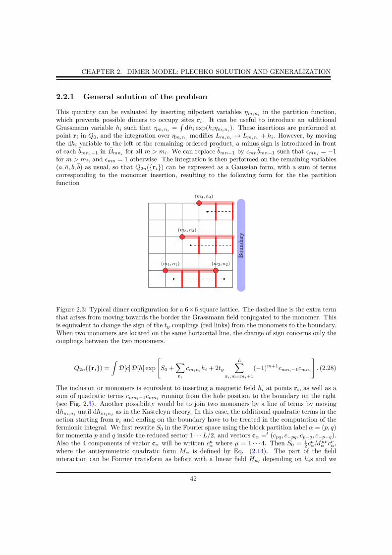
CHAPTER 2. DIMER MODEL: PLECHKO SOLUTION AND GENERALIZATION
2.2.1 General solution of the problem
This quantity can be evaluated by inserting nilpotent variables ηminiin the partition function,
which prevents possible dimers to occupy sites ri. It can be useful to introduce an additionalGrassmann variable hi such that ηmini
=∫
dhi exp(hiηmini). These insertions are performed at
point ri in Q0, and the integration over ηminimodifies Lmini
→ Lmini+ hi. However, by moving
the dhi variable to the left of the remaining ordered product, a minus sign is introduced in frontof each bmni−1 in Bmni
for all m > mi. We can replace bmn−1 by ǫmnbmn−1 such that ǫmni= −1
for m > mi, and ǫmn = 1 otherwise. The integration is then performed on the remaining variables(a, a, b, b) as usual, so that Q2n({ri}) can be expressed as a Gaussian form, with a sum of termscorresponding to the monomer insertion, resulting to the following form for the the partitionfunction
(m1, n1)
(m4, n4)
(m3, n3)
(m2, n2)
Bou
ndary
Figure 2.3: Typical dimer configuration for a 6×6 square lattice. The dashed line is the extra termthat arises from moving towards the border the Grassmann field conjugated to the monomer. Thisis equivalent to change the sign of the ty couplings (red links) from the monomers to the boundary.When two monomers are located on the same horizontal line, the change of sign concerns only thecouplings between the two monomers.
Q2n({ri}) =
∫D[c] D[h] exp
[S0 +
∑
ri
cminihi + 2ty
L∑
ri,m=mi+1
(−1)m+1cmni−1cmni
]. (2.28)
The inclusion or monomers is equivalent to inserting a magnetic field hi at points ri, as well as asum of quadratic terms cmni−1cmni
running from the hole position to the boundary on the right(see Fig. 2.3). Another possibility would be to join two monomers by a line of terms by movingdhmini
until dhmjnjas in the Kasteleyn theory. In this case, the additional quadratic terms in the
action starting from ri and ending on the boundary have to be treated in the computation of thefermionic integral. We first rewrite S0 in the Fourier space using the block partition label α = (p, q)for momenta p and q inside the reduced sector 1 · · ·L/2, and vectors cα =t (cpq, c−pq, cp−q, c−p−q).Also the 4 components of vector cα will be written cµα where µ = 1 · · · 4. Then S0 = i
2cµαM
µνα cνα,
where the antisymmetric quadratic form Mα is defined by Eq. (2.14). The part of the fieldinteraction can be Fourier transform as before with a linear field Hpq depending on his and we
42

CHAPTER 2. DIMER MODEL: PLECHKO SOLUTION AND GENERALIZATION
obtain
∑
ri
cmi,nihi =
L∑
p,q=1
cpqHpq =∑
α,µ
cµαHµα . (2.29)
The last contribution connecting the monomers to the boundary can be written as i2cµαV
µναβ c
νβ , with
matrix Vαβ = Vpq,p′q′ given by
Vpq,p′q′ =∑
ri
8ty(−1)ni
(L+ 1)2
{L∑
m=mi+1
sinπpm
L+ 1sin
πp′m
L+ 1
}[sin
πq(ni − 1)
L+ 1sin
πq′niL+ 1
− (q ↔ q′)
].
The different components V µναβ are given implicitly, for the first elements, by V 11αβ = Vpq,p′q′ , V 12
αβ =
Vpq,−p′q′ , V 21αβ = V−pq,p′q′ , and so on. Then the total fermionic action contains three terms
S =i
2cµαM
µνα cνα +
i
2cµαV
µναβ c
νβ + cµαH
µα . (2.30)
The first two terms contain only modes of the same sector α, and the last connects modes fromdifferent sectors α and β. Matrices Mµν
α and V µναβ are antisymmetric: Mµνα = −Mνµ
α and V µναβ =
−V νµβα . Also Vαα = 0. Then the quantity Q2n({ri}) can be formally written as
Q2n({ri}) =
∫D[c] D[h] exp
(i
2cµα[Mµν
α δαβ + V µναβ ]cνβ + cµαHµα
)
=
∫D[c] D[h] exp
(i
2cµαW
µναβ c
νβ + cµαH
µα
), (2.31)
with Wµναβ = δαβM
µνα + V µναβ (cf. Fig. 2.4(a)). By construction, W is antisymmetric and satisfies
Wµναβ = −W νµ
βα . This matrix can be represented as a block matrix of global size L2 × L2
W =
Mα=(1,1) V(1,1),(1,2) V(1,1),(1,3) · · ·︸ ︷︷ ︸
4×4 matrix
−V(1,1),(1,2) M(1,2) V(1,2),(1,3) · · ·−V(1,1),(1,3) −V(1,2),(1,3) M(1,3) · · ·
...
︸ ︷︷ ︸L2/4 blocks
(2.32)
where each of the (L2/4) × (L2/4) blocks is a 4 × 4 matrix. Labels α are ordered with increasingmomentum (1, 1), (1, 2) · · · (1, L/2), (2, 1) · · · In the action the linear terms in cµα can be removedusing a linear change of variables cµα → cµα + gµα, where gµα are Grassmann constants. After somealgebra, we find the correct values for the constants that eliminate the linear contribution are givenby gµα = i(W−1)µναβH
νβ . After substitution of these values in the overall integral, and a rescaling of
variables cα → cα/√i, the action becomes a product over variables c and hi
Q2n({ri}) =
∫D[c] D[h] exp
[1
2cµαW
µναβ c
νβ − i
2(W−1)µναβH
µαH
νβ
]
= pf(W )
∫D[h] exp
[− i
2(W−1)µναβH
µαH
νβ
].
43

CHAPTER 2. DIMER MODEL: PLECHKO SOLUTION AND GENERALIZATION
The fields Hµα can be expressed with hi as Hµ
α =∑2ni=1 Λµi,αhi, where coefficients Λµi,α can be
rewritten using a 4-dimensional vector, such as
Λi,α =2
L+ 1sin
πpmi
L+ 1sin
πqniL+ 1
Λi =: ri(α)Λi, (2.33)
where the vector
Λi =
imi+ni
−i−mi+ni
−imi−ni
i−mi−ni
, (2.34)
depends only on the location parity of the monomer ri in the bulk. Functions ri(α) are normalized∑α ri(α)rj(α) = δij . Then we obtain the following formal and compact expression for Q2n({ri})
Q2n({ri}) = pf(W )
∫D[h] exp
1
2
∑
i,j
hihjΛµi,α(W−1)µναβΛνj,β
=: pf(W )
∫D[h] exp
1
2
∑
i,j
hihjCij
. (2.35)
Finally, we found a pfaffian expression of the partition function
Q2n({ri}) = pf(W )pf(C), (2.36)
where C is a real (2n× 2n) antisymmetric matrix with elements Cij = Λµi,α(W−1)µναβΛνj,β . It is alsoworth noting that we have a similar structure in the real space, where the total action Eq. (5.9)is expressed by S = 1
2cmnWmn,m′n′cm′n′ +∑
ricmini
hi, with W containing both the connectivitymatrix M and the contribution of the line of defects V . A direct computation also leads to thefactorization Qn({ri}) = pf(W )pf(C), where Cij = (W−1)mini,mjnj
is a (n × n) antisymmetricmatrix.
44

CHAPTER 2. DIMER MODEL: PLECHKO SOLUTION AND GENERALIZATION
• The size of the matrix grow linearly with the number of monomers dimC = 2n×2nand Cij = 0 if ni and nj have the same parity.
• We verify easily that the matrix Cij is antisymmetric by using the antisymmetryproperty of W
Cji = Λµj,α(W−1)µναβΛνi,β
= Λνj,β(W−1)νµβαΛµi,α
= − Λνj,β(W−1)µναβΛµi,α= − Cij .
Then, Cij can be formally expressed as a scalar product
Cij =∑
α,β
⟨Λi,α|W−1
α,β |Λj,β
⟩.
Box 4 (Properties of the matrix C).
Q2n is therefore a product of two pfaffians where the monomer locations are specified in matrix W .The matrix V can be rewritten using additional matrices after considering the different components
omèr
(a) (b)
10 5020 3015
104
0.001
0.005
0.010
0.050
60. 65. 70. 75.
0.028
0.029
0.03
0.031
0.032
0.033
0.034
0.035
Figure 2.4: (a) Graphical representation of the matrix W = M + V . (b) When the monomers areon the boundaries of the domain, the off diagonal term V vanishes and the matrix W reduces tothe matrix M .
(µ, ν). We can indeed express V using four functions ua,sk (α, β), and va,sk (α, β), for each monomerat location rk = (mk, nk), with mk < L, and such that
Vαβ = − 2ty∑
rk
∑
c,c′
uck(α, β)Γcc′vc′
k (α, β), (2.37)
45
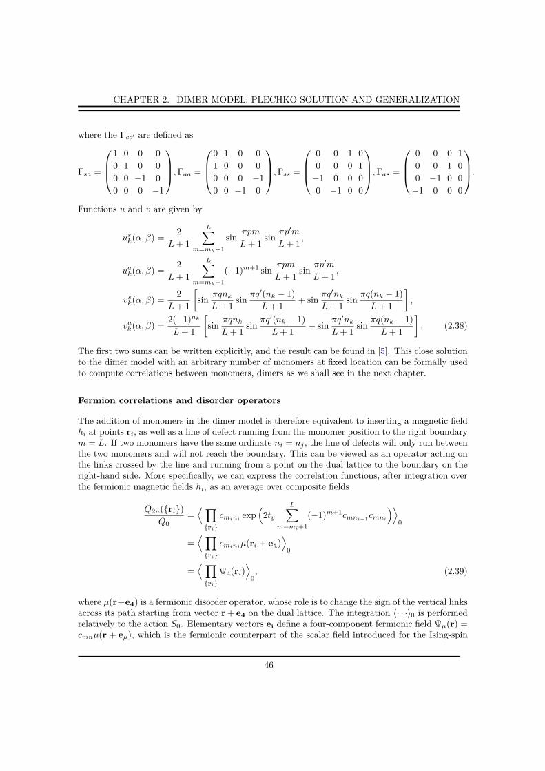
CHAPTER 2. DIMER MODEL: PLECHKO SOLUTION AND GENERALIZATION
where the Γcc′ are defined as
Γsa =
1 0 0 0
0 1 0 0
0 0 −1 0
0 0 0 −1
,Γaa =
0 1 0 0
1 0 0 0
0 0 0 −1
0 0 −1 0
,Γss =
0 0 1 0
0 0 0 1
−1 0 0 0
0 −1 0 0
,Γas =
0 0 0 1
0 0 1 0
0 −1 0 0
−1 0 0 0
.
Functions u and v are given by
usk(α, β) =2
L+ 1
L∑
m=mk+1
sinπpm
L+ 1sin
πp′m
L+ 1,
uak(α, β) =2
L+ 1
L∑
m=mk+1
(−1)m+1 sinπpm
L+ 1sin
πp′m
L+ 1,
vsk(α, β) =2
L+ 1
[sin
πqnkL+ 1
sinπq′(nk − 1)
L+ 1+ sin
πq′nkL+ 1
sinπq(nk − 1)
L+ 1
],
vak(α, β) =2(−1)nk
L+ 1
[sin
πqnkL+ 1
sinπq′(nk − 1)
L+ 1− sin
πq′nkL+ 1
sinπq(nk − 1)
L+ 1
]. (2.38)
The first two sums can be written explicitly, and the result can be found in [5]. This close solutionto the dimer model with an arbitrary number of monomers at fixed location can be formally usedto compute correlations between monomers, dimers as we shall see in the next chapter.
Fermion correlations and disorder operators
The addition of monomers in the dimer model is therefore equivalent to inserting a magnetic fieldhi at points ri, as well as a line of defect running from the monomer position to the right boundarym = L. If two monomers have the same ordinate ni = nj , the line of defects will only run betweenthe two monomers and will not reach the boundary. This can be viewed as an operator acting onthe links crossed by the line and running from a point on the dual lattice to the boundary on theright-hand side. More specifically, we can express the correlation functions, after integration overthe fermionic magnetic fields hi, as an average over composite fields
Q2n({ri})Q0
=⟨∏
{ri}
cminiexp
(2ty
L∑
m=mi+1
(−1)m+1cmni−1cmni
)⟩0
=⟨∏
{ri}
cminiµ(ri + e4)
⟩0
=⟨∏
{ri}
Ψ4(ri)⟩
0, (2.39)
where µ(r+e4) is a fermionic disorder operator, whose role is to change the sign of the vertical linksacross its path starting from vector r + e4 on the dual lattice. The integration 〈· · ·〉0 is performedrelatively to the action S0. Elementary vectors ei define a four-component fermionic field Ψµ(r) =cmnµ(r + eµ), which is the fermionic counterpart of the scalar field introduced for the Ising-spin
46
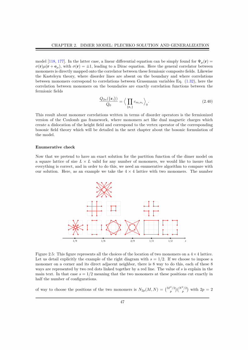
CHAPTER 2. DIMER MODEL: PLECHKO SOLUTION AND GENERALIZATION
model [118, 177]. In the latter case, a linear differential equation can be simply found for Ψµ(r) =σ(r)µ(r + eµ), with σ(r) = ±1, leading to a Dirac equation. Here the general correlator betweenmonomers is directly mapped onto the correlator between these fermionic composite fields. Likewisethe Kasteleyn theory, where disorder lines are absent on the boundary and where correlationsbetween monomers correspond to correlations between Grassmann variables Eq. (1.32), here thecorrelation between monomers on the boundaries are exactly correlation functions between thefermionic fields
Q2n({ri})Q0
=⟨∏
{ri}
cmini
⟩0. (2.40)
This result about monomer correlations written in terms of disorder operators is the fermionizedversion of the Coulomb gas framework, where monomers act like dual magnetic charges whichcreate a dislocation of the height field and correspond to the vertex operator of the correspondingbosonic field theory which will be detailed in the next chapter about the bosonic formulation ofthe model.
Enumerative check
Now that we pretend to have an exact solution for the partition function of the dimer model ona square lattice of size L × L valid for any number of monomers, we would like to insure thateverything is correct, and in order to do this, we need an enumerative algorithm to compare withour solution. Here, as an example we take the 4 × 4 lattice with two monomers. The number
s1/9 1/6 2/9 1/3 1/2
Figure 2.5: This figure represents all the choices of the location of two monomers on a 4×4 lattice.Let us detail explicitly the example of the right diagram with s = 1/2. If we choose to impose amonomer on a corner and its direct adjacent neighbor, there is 8 way to do this, each of these 8ways are represented by two red dots linked together by a red line. The value of s is explain in themain text. In that case s = 1/2 meaning that the two monomers at these positions cut exactly inhalf the number of configurations.
of way to choose the positions of the two monomers is N2p(M,N) =(M2/2p
)(N2/2p
)with 2p = 2
47

CHAPTER 2. DIMER MODEL: PLECHKO SOLUTION AND GENERALIZATION
and M = N = 2 then N2(4, 4) = 64. We can define a number s which will be the ratio of thepartition function Q0 without monomers (36 in that case) by the partition function Q2 with twomonomers at fixed positions. This quantity will be a rational number ∈ [1/2, 0[ for any size latticeand is completely defined by the matrices W and C written above. The results shown in Fig. 2.5completely agree with enumeration algorithms2, confirming the exactness of our solution. We sawin the previous paragraph that this quantity is simply the correlation function Cij between thetwo monomers which becomes a lot simpler in the case where there are on the boundaries of thedomain.
2.2.2 Boundary monomers and 1d complex fermion chain
As we have seen before, the correlation between monomers become much more simpler in the casewhere there are restricted to live on the boundaries of the lattice. In this section we shall studythese correlations and try to extract a closed expression starting to the case where the monomersare on the same boundary (Fig. 2.10(a)). The generalization of different boundaries (Fig. 2.10(b,c))is much more tricky but we will see that a compact closed formula is also available.
Monomers on the same boundary
Although the general problem remains in principle tractable, we can simplify it further by consider-ing monomers on the boundary mi = L of the rectangle only, with the convention ni > nj if i > j.When the monomers are on the boundaries of the domain, the off diagonal term V vanishes andthe matrix W reduces to the matrix M (cf. Fig. 2.4(b)). In that case, the previous action contains
(a) (b) (c)
Figure 2.6: The three different possibilities of two monomer’s location. (a) on a same boundary(b) on adjacent boundaries or (c) on opposite boundaries.
no defect line term, only the couplings with fields remain and the problem can be transformed intoa 1d system of particles on a chain (see Fig. 2.7). Using the previous Fourier transform for the c’s
2For this small size, it can be check by hands
48

CHAPTER 2. DIMER MODEL: PLECHKO SOLUTION AND GENERALIZATION
variables, the magnetic field term becomes
∑
ri
cmi,nihi =
L∑
p,q=1
cpqHpq,
Hpq =∑
ri
2imi+ni
L+ 1sin
πpmi
L+ 1sin
πqniL+ 1
hi. (2.41)
Then the partition function can be integrated on the cmn’s using the block partition (p, q) and wefind that
Q2n({ri}) = Q0
∫dh1 · · ·dh2n expSH , (2.42)
where
SH =
L/2∑
p,q=1
itx cos πpL+1 (Hp−qH−pq +HpqH−p−q) + ity cos πq
L+1 (H−pqH−p−q +HpqHp−q)
2t2x cos2 πpL+1 + 2t2y cos2 πq
L+1
.
Grassmann fields Hpq has the following properties: H−pq = −Hpq and H−p−q = −Hp−q. In
Cij
ni nj
Figure 2.7: Configuration of 2 monomers on the boundary at the position ni and nj correlated byCij . This correlation decreases as the inverse of the distance and vanishes if ni and nj have thesame parity.
that case, the first sum on the right hand side of the previous equation vanishes due to the anti-commuting property, and we can reduce the field-dependent action to one single sum
SH =′∑
p,q=1
ity cos πqL+1
t2x cos2 πpL+1 + t2y cos2 πq
L+1
HpqHp−q, (2.43)
where the prime symbol is meant for summation over half of the modes p, q = 1 · · ·L/2. This actionwould vanish if all the ni were for example even, since the Grassmann fields satisfy in this caseHpqHp−q = −H2
pq = 0. In general, the field action can be rewritten as a quadratic form over the
real-space fields hi: SH =∑i<j Cijhihj , where the elements of the matrix C are antisymmetric
Cij = −Cji, and equal to
Cij(L) =4 [(−1)ni − (−1)nj ]
(L+ 1)2
L/2∑
p,q=1
i1+ni+nj ty cos πqL+1 sin2 πp
L+1
t2x cos2 πpL+1 + t2y cos2 πq
L+1
sinπqniL+ 1
sinπqnjL+ 1
(2.44)
49

CHAPTER 2. DIMER MODEL: PLECHKO SOLUTION AND GENERALIZATION
These elements are zero if ni and nj have the same parity and in general the integration overthe field variables hi leads directly to a pfaffian form for the partition function Q2n({ri}) =Q0(−1)npf(C). The (−1)n factor comes from the rearrangement of the measure dh1 · · ·dh2n =(−1)n dh2n · · ·dh1, so that the 2n-function reads
∫ 2n∏
i=1
dhi exp
−
∑
i<j
Cijhihj
= pf(C). (2.45)
This sign could also be absorbed in the definition of matrix elements Cij → −Cij . The resultingpartition function is always positive with this definition. For example, if there are 2 monomersat the boundary, pf(C) = −C12, and 4 monomers3 leads to pf(C) = C12C34 − C13C24 + C14C23
(cf. Fig. 2.8). Cij are zero if ni and nj > ni have the same parity. In the case n1 = L/2− k and
pf(C) =n1 n2
pf(C) =n1 n2 n3 n4
− +n1 n2 n3 n4 n1 n2 n3 n4
pf(C) = − +n1 n2 n3 n4 n5 n6 n1 n2 n3 n4 n5 n6
− +...n1 n2 n3 n4 n5 n6 n1 n2 n3 n4 n5 n6
.
Figure 2.8: Diagrammatical representation of the pfaffian of C for 2, 4 and 6 monomers
n2 = L/2 + k + 1, C12 ≃ 2π r
−1 − 2π r
−3 instead, with r = 2k + 1 and amplitude 2/π. This resultis in agreement with the work of Priezzhev and Ruelle [178] on the scaling limit of the correlationfunctions of boundary monomers in a system of closely packed dimers in terms of a 1d chiral freefermion theory. We should notice that the expression Eq. (2.44) is an exact closed expression forthe 2-point correlation between monomers on the boundary mi = mj = L, leading to an explicitresult for the partition function with 2, 4...2n monomers. We will show in a next section how tofind the correlation between monomers on different (opposite or adjacent) boundaries of the lattice.
General case
In the case where the monomers are on the boundaries, we were able to compute exactly the 2-pointcorrelation function Eq. (2.44) in the discrete case. In the bulk case, the things are much morecomplicated and an exact closed-form expression on the discrete level seems hard. Nevertheless,a perturbative expansion can be performed to evaluate the pfaffian expression of the correlation
3As a straightforward application, the number of perfect matching with a monomer on each corner can becomputed and the result is Qcorner
4 = {1, 8, 784, 913952, 1211936774...}
50
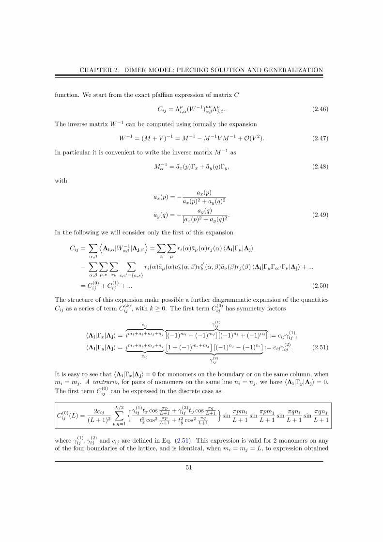
CHAPTER 2. DIMER MODEL: PLECHKO SOLUTION AND GENERALIZATION
function. We start from the exact pfaffian expression of matrix C
Cij = Λµi,α(W−1)µναβΛνj,β . (2.46)
The inverse matrix W−1 can be computed using formally the expansion
W−1 = (M + V )−1 = M−1 −M−1VM−1 +O(V 2). (2.47)
In particular it is convenient to write the inverse matrix M−1 as
M−1α = ax(p)Γx + ay(q)Γy, (2.48)
with
ax(p) = − ax(p)
ax(p)2 + ay(q)2
ay(q) = − ay(q)
[ax(p)2 + ay(q)2. (2.49)
In the following we will consider only the first of this expansion
Cij =∑
α,β
⟨Λi,α|W−1
αβ |Λj,β
⟩=∑
α
∑
µ
ri(α)aµ(α)rj(α) 〈Λi|Γµ|Λj〉
−∑
α,β
∑
µ,ν
∑
rk
∑
c,c′={a,s}
ri(α)aµ(α)uck(α, β)vc′
k (α, β)aν(β)rj(β) 〈Λi|ΓµΓcc′Γν |Λj〉+ ...
= C(0)ij + C
(1)ij + ... (2.50)
The structure of this expansion make possible a further diagrammatic expansion of the quantities
Cij as a series of term C(k)ij , with k ≥ 0. The first term C
(0)ij has symmetry factors
〈Λi|Γx|Λj〉 =
cij︷ ︸︸ ︷imi+ni+mj+nj
γ(1)ij︷ ︸︸ ︷
[(−1)mi − (−1)mj ] [(−1)ni + (−1)nj ] := cijγ(1)ij ,
〈Λi|Γy|Λj〉 = imi+ni+mj+nj︸ ︷︷ ︸cij
[1 + (−1)mi+mj
][(−1)nj − (−1)ni ]
︸ ︷︷ ︸γ
(2)ij
:= cijγ(2)ij . (2.51)
It is easy to see that 〈Λi|Γx|Λj〉 = 0 for monomers on the boundary or on the same column, whenmi = mj . A contrario, for pairs of monomers on the same line ni = nj , we have 〈Λi|Γy|Λj〉 = 0.
The first term C(0)ij can be expressed in the discrete case as
C(0)ij (L) =
2cij(L+ 1)2
L/2∑
p,q=1
{γ(1)ij tx cos πp
L+1 + γ(2)ij ty cos πq
L+1
t2x cos2 πpL+1 + t2y cos2 πq
L+1
}sin
πpmi
L+ 1sin
πpmj
L+ 1sin
πqniL+ 1
sinπqnjL+ 1
where γ(1)ij , γ
(2)ij and cij are defined in Eq. (2.51). This expression is valid for 2 monomers on any
of the four boundaries of the lattice, and is identical, when mi = mj = L, to expression obtained
51
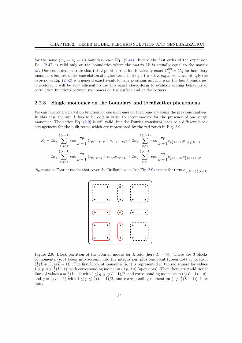
CHAPTER 2. DIMER MODEL: PLECHKO SOLUTION AND GENERALIZATION
for the same (mi = ni = L) boundary case Eq. (2.44). Indeed the first order of the expansionEq. (2.47) is valid only on the boundaries where the matrix W is actually equal to the matrix
M . One could demonstrate that this 2-point correlation is actually exact C(0)ij = Cij for boundary
monomers because of the cancelation of higher terms in the perturbative expansion, accordingly theexpression Eq. (2.52) is a general exact result for any positions anywhere on the four boundaries.Therefore, it will be very efficient to use this exact closed-form to evaluate scaling behaviors ofcorrelation functions between monomers on the surface and at the corners.
2.2.3 Single monomer on the boundary and localization phenomena
We can recover the partition function for one monomer on the boundary using the previous analysis.In this case the size L has to be odd in order to accommodate for the presence of one singlemonomer. The action Eq. (2.9) is still valid, but the Fourier transform leads to a different blockarrangement for the bulk terms which are represented by the red zones in Fig. 2.9
S0 = 2itx
12 (L−1)∑
p,q≥1
cosπp
L+ 1(cpqc−p−q + cp−qc−pq) + 2itx
12 (L−1)∑
p≥1
cosπp
L+ 1cp 1
2 (L+1)c−p 12 (L+1)
+ 2ity
12 (L−1)∑
p,q≥1
cosπq
L+ 1(cpqcp−q + c−pqc−p−q) + 2ity
12 (L−1)∑
q≥1
cosπq
L+ 1c 1
2 (L+1)qc 12 (L+1)−q.
S0 contains Fourier modes that cover the Brillouin zone (see Fig. 2.9) except for term c 12 (L+1) 1
2 (L+1)
Figure 2.9: Block partition of the Fourier modes for L odd (here L = 5). There are 3 blocksof momenta (p, q) taken into account into the integration, plus one point (green dot) at location( 1
2 (L+ 1), 12 (L+ 1)). The first block of momenta (p, q) is represented in the red square for values
1 ≤ p, q ≤ 12 (L−1), with corresponding momenta (±p,±q) (open dots). Then there are 2 additional
lines of values p = 12 (L−1) with 1 ≤ q ≤ 1
2 (L−1)/2, and corresponding momentum (12 (L−1),−q),
and q = 12 (L − 1) with 1 ≤ p ≤ 1
2 (L − 1)/2, and corresponding momentum (−p, 12 (L − 1)), blue
dots.
52

CHAPTER 2. DIMER MODEL: PLECHKO SOLUTION AND GENERALIZATION
which is located in the middle of the zone and not present in the sums Eq. (2.52). The integrationover Grassmann variables cpq is therefore zero in absence of coupling with this mode. Inserting asingle monomer on the boundary at location r = (L, n) is equivalent, as previously demonstrated,to inserting a Grassmann field h and a field contribution SH = cLnh in the action, which can beexpanded using Fourier transformation
SH =2iL+n
L+ 1
∑
p,q
(−1)p+1 sinπp
L+ 1sin
πqn
L+ 1cpqh
=∑
p,q
cpqHpq. (2.52)
Since there is only one Grassmann field, all terms Hpq are only proportional to h, and there-fore the quadratic form in Eq. (2.43) is zero. However one term contributes to the integrationover c 1
2 (L+1) 12 (L+1), and corresponds to c 1
2 (L+1) 12 (L+1)H 1
2 (L+1) 12 (L+1). After integration over the
remaining cpq and h variables, the partition function can then be factorized as
Q1 =−2in+1 sin(πn/2)
L+ 1
12 (L−1)∏
p,q=1
[4t2x cos2 πp
L+ 1+ 4t2y cos2 πq
L+ 1
] 12 (L−1)∏
p=1
2tx cosπp
L+ 1
12 (L−1)∏
q=1
2ty cosπq
L+ 1.
This result is consistent to the fact that a monomer can be put only at odd site locations. We can
use the formula∏ 1
2 (L−1)p=1 2 cos( πp
L+1 ) =√
L+12 , to simplify the previous expression and recover the
Tzeng-Wu [202] solution that we have showed in the first chapter
Q1 =
12 (L−1)∏
p,q=1
[4t2x cos2 πp
L+ 1+ 4t2y cos2 πq
L+ 1
]× (txty)
12 (L−1) × [−in+1 sin(πn/2)]. (2.53)
This solution will be used in the next chapter to extract finite-size scaling behavior of the freeenergy in a CFT framework, where boundary changing conditions operators has to be carefullystudy to infer the central charge of the model in the context of the height mapping formulation.
Localization phenomena
We can notice that the partition function with one monomer in a system of size L× L (L odd) isequal to the partition function without monomers on a lattice of size L−1×L−1. The probabilityis therefore constant for all location of the monomer, at even sites only, the last term in bracketbeing equal to zero (n odd) or unity (n even), proving that the monomer is fully delocalized onthe boundary, unlike the bulk case where monomers are actually localized in a finite region of thedomain [27, 174]. Actually it has been shown that the delocalization probability, i.e. the probabilitythat the vacancy can reach the boundary of the square lattice, decay with the system size as L−1/4
and moreover the analyze of the distribution p(s) for the size s of the domain accessible to themonomer in an infinite system has been studied in the context of spanning webs and has beenshown to decrease a p(s) ∼ s−9/8. The same kind of analysis has been done for the triangularlattice [111].
53
CHAPTER 2. DIMER MODEL: PLECHKO SOLUTION AND GENERALIZATION
2.3 Fun with dimers
In this section, one shows a curious combinatorial analogy between the partition function of theclose packing dimer model on a L × L square lattice with open boundary conditions, and thesame partition function with boundary monomers. One start reminding some properties of thepure dimer model partition function, and we show, thanks to our exact calculation of the partitionfunction with 2n monomers, that this analogy can be understood and demonstrated. Hereinafter,the Boltzmann weights tx and ty are taken to be the unity in such way that the partition functionis exactly equal to the perfect matching number. All the results presented in this section has beenchecked with depth-first [144] algorithms up to size L = 10. For bigger sizes, Monte-Carlo ortransfer matrix simulations [145] has to be implement.
2.3.1 Partition function without monomers
The partition function of the pure dimer model on a M ×N lattice with open boundary conditionsis
Q0(M,N) =
M/2∏
p=1
N/2∏
q=1
[4 cos2 πp
M + 1+ 4 cos2 πq
N + 1
], (2.54)
which can be written for the special case of the square geometry M = N = L
Q0(L) = 2L/2.g2L/2 (2.55)
where gL/2 is a number sequence (OEIS A065072) 4 equal, for L = 2, 4, 6, 8, 10, 12, 14..., to
gL/2 = {1, 3, 29, 901, 89893, 28793575, 29607089625...}.The resulting sequence for the partition function is then (OEIS A004003) for L = 2, 4, 6, 8, 10, 12, 14
Q0 = {2, 36, 6728, 12988816, 258584046368, 53060477521960000, 112202208776036178000000...}.For example, the number of configurations of dimers on the chessboard (L = 8) is Q0(8) = 24g2
4 =24×9012 = 12988816 as previously noticed by Fisher [71]. Another observation is that the numberof configuration on the square L× L is always even.
It is less trivial to notice that {gp} is a sequence of odd number satisfying the relation
gp = p+ 1(mod 32) if p even
= (−1)(p−1)/2 × p(mod 32) if p odd. (2.56)
The proof of this statement can be found in the original paper [117]. The exact solutionof the dimer model with one boundary monomer allows for the same kind of numbertheory analysis (cf. [138] for details).
Box 5 (Number theory curiosity).
4The On-Line Encyclopedia of Integer Sequences https://oeis.org/
54
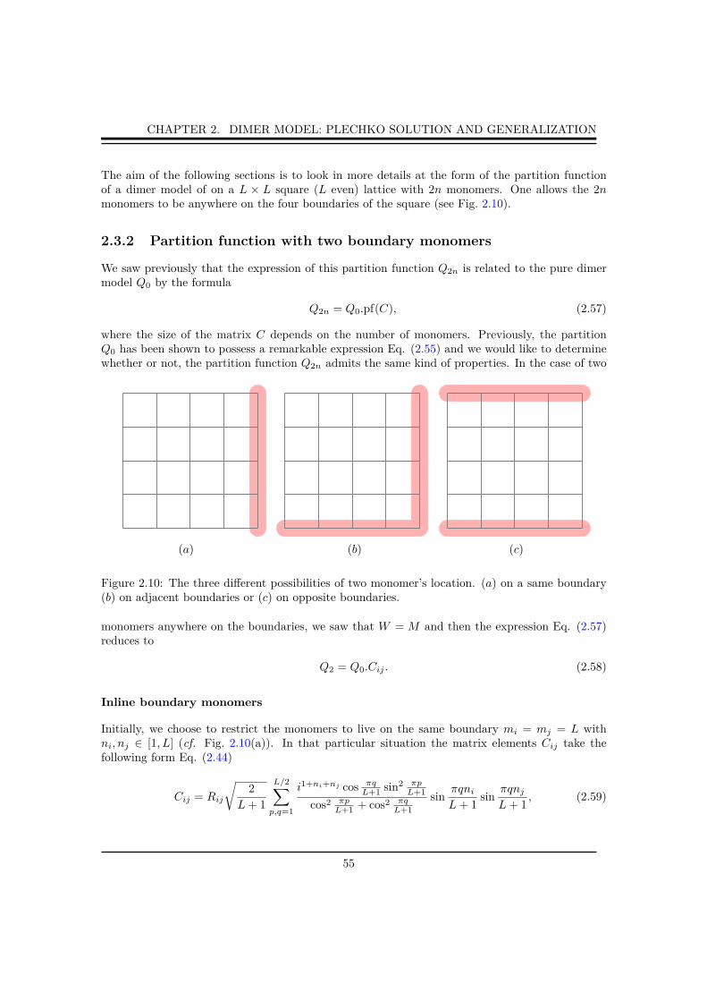
CHAPTER 2. DIMER MODEL: PLECHKO SOLUTION AND GENERALIZATION
The aim of the following sections is to look in more details at the form of the partition functionof a dimer model of on a L × L square (L even) lattice with 2n monomers. One allows the 2nmonomers to be anywhere on the four boundaries of the square (see Fig. 2.10).
2.3.2 Partition function with two boundary monomers
We saw previously that the expression of this partition function Q2n is related to the pure dimermodel Q0 by the formula
Q2n = Q0.pf(C), (2.57)
where the size of the matrix C depends on the number of monomers. Previously, the partitionQ0 has been shown to possess a remarkable expression Eq. (2.55) and we would like to determinewhether or not, the partition function Q2n admits the same kind of properties. In the case of two
(a) (b) (c)
Figure 2.10: The three different possibilities of two monomer’s location. (a) on a same boundary(b) on adjacent boundaries or (c) on opposite boundaries.
monomers anywhere on the boundaries, we saw that W = M and then the expression Eq. (2.57)reduces to
Q2 = Q0.Cij . (2.58)
Inline boundary monomers
Initially, we choose to restrict the monomers to live on the same boundary mi = mj = L withni, nj ∈ [1, L] (cf. Fig. 2.10(a)). In that particular situation the matrix elements Cij take thefollowing form Eq. (2.44)
Cij = Rij
√2
L+ 1
L/2∑
p,q=1
i1+ni+nj cos πqL+1 sin2 πp
L+1
cos2 πpL+1 + cos2 πq
L+1
sinπqniL+ 1
sinπqnjL+ 1
, (2.59)
55

CHAPTER 2. DIMER MODEL: PLECHKO SOLUTION AND GENERALIZATION
where
Rij = ± 2 if ni ∈ Z2p(Z2p+1) and nj ∈ Z2p(Z2p+1)
= 0 if ni ∈ Z2p and nj ∈ Z2p+1 or converserly. (2.60)
In table 2.1, we evaluate this expression using Mathematicar, restricting one monomer to be in
nj = 1 and the second to be between 1 to L for several system sizes. One can observe that there
Cij(L) 4 6 8 10 12 14(1, 1), (2, 1) 1/2 1/2 1/2 1/2 1/2 1/2(1, 1), (4, 1) 1/3 9/29 275/901 27293/89893 8724245/28793575 8962349805/29607089625(1, 1), (6, 1) . 7/29 199/901 19279/89893 6103405/28793575 6242309595/29607089625(1, 1), (8, 1) . . 169/901 15395/89893 4750015/28793575 4800013155/29607089625(1, 1), (10, 1) . . . 13761/89893 4036195/28793575 3979640565/29607089625(1, 1), (12, 1) . . . . 3721985/28793575 3520442385/29607089625(1, 1), (14, 1) . . . . . 3311911215/29607089625
gL/2 3 29 901 89893 28793575 29607089625
Table 2.1: Correlation function Cij for a boundary monomer (mi = mj = L) fixed on the first sitenj = 1 as function of the ordinate ni for several system sizes L (see Fig. 2.10(a)). The value ofCij where the two monomers are on the corner (1, 1), (2, 1) is always equal to 1/2, because it isequivalent to force a dimer to be on the corner and then split the number of configuration by two.Bottom line: Values of the sequence gL for L = 4..14.
is a curious relation between the expression Cij and the sequence gL/2 present in the partitionfunction Q0, more precisely one can deduce a proportionality relation
Cij(L) ∝ g−1L/2, (2.61)
which appears to be valid for all system sizes L in the case of inline monomers.
General case
The general expression of the matrix elements of the correlations between boundary monomers Eq.(2.52), valid in all the geometries of Fig. 2.10 can be written as
Cij =2cij
(L+ 1)2
L/2∑
p,q=1
{ γ(1)ij cos πp
L+1
t2x cos2 πpL+1 + t2y cos2 πq
L+1
+γ
(2)ij cos πq
L+1
t2x cos2 πpL+1 + t2y cos2 πq
L+1
}
× sinπpmi
L+ 1sin
πpmj
L+ 1sin
πqniL+ 1
sinπqnjL+ 1
, (2.62)
where γ(1)ij , γ
(2)ij and cij are defined in Eq. (2.51). In table 2.2 , we evaluate this expression for
the two other geometries. The same relation holds in this case as well, and we conjecture that theexpression of the 2-point correlation takes the following form
Cij(L) = α(2)ij (L)g−1
L/2, (2.63)
56

CHAPTER 2. DIMER MODEL: PLECHKO SOLUTION AND GENERALIZATION
Cij(L) 4 6 8 10 12(1, 1), (L, 1) 1/3 7/29 169/901 13761/89893 3721985/28793575(1, 1), (L, 3) 1/(2× 3) 5/29 138/901 12127/89893 3407775/28793575(1, 1), (L, 5) . 5/(2× 29) 95/901 9475/89893 2864755/28793575(1, 1), (L, 7) . . 95/(2× 901) 6389/89893 2194565/28793575(1, 1), (L, 9) . . . 6389/(2× 89893) 1471805/28793575(1, 1), (L, 11) . . . . 1471805/(2× 28793575)
Cij(L) 4 6 8 10 12(1, 1), (L, 1) 1/3 7/29 169/901 13761/89893 3721985/28793575(1, 2), (L, 2) 1/6 2/29 30/901 1634/89893 314210/28793575(1, 3), (L, 3) 1/6 9/29 125/901 11109/89893 3178965/28793575(1, 4), (L, 4) 1/3 9/29 155/901 4720/89893 984400/28793575
gL/2 3 29 901 89893 28793575
Table 2.2: Top: Correlation function Cij between a monomer at position (mi = ni = 1) and anotherat position (mj = L, nj) for several system sizes L and for nj = 1, 3, 5, 7, 9, 11 (cf. Fig. 2.10(b)). Wenote that the expression of the last line in each row is the half of the expression of the penultimateline. Bottom: Correlation function Cij between opposite side monomers for several system sizes Land for ni = nj = 1, 2, 3, 4 (see Fig. 2.10(c)).
no matter the positions of the two monomers on the boundaries, where α(2)ij depends only of the
positions of the two monomers and of the system size L. We did not succeed to prove this equalitybetween a double product (gL/2 define by Eq. (2.55) ) and a double sum (Cij(L) defined by Eq.(2.62)), but there is, numerically speaking, absolutely no-doubt that is true. Considering thatrelation valid, the partition function of the dimer model with two boundary monomers reads
Q2(L) = α(2)ij (L).gL/2 (2.64)
2.3.3 Partition function with 2n boundary monomers
It is worth looking at higher number of monomers to conjecture a more general form of the partitionfunction. We have conjectured that the matrix elements of the correlation matrix are proportionalto the sequence gL/2, thus thanks to the general pfaffian solution with 2n monomers Eq. (2.57),we obtains the formulas
Q2 = Q0.Cij ,
Q4 = Q0.(CijCkl − CikCjl + CilCjk
),
Q6 = Q0.(CijCklCmn − CilCjlCmn + CilCjmCkn − ...
), (2.65)
...
57
CHAPTER 2. DIMER MODEL: PLECHKO SOLUTION AND GENERALIZATION
where the pure partition function takes the form Eq. (2.55), therefore the partition functions areproportional to power of gL/2
Q0(L) = 2L/2.g2L/2,
Q2(L) = α(2)ij (L).gL/2,
Q4(L) = α(4)ijkl(L).g0
L/2,
Q6(L) = α(6)ijklmn(L).g−1
L/2, (2.66)
...
which can be generalized for 2n monomers at positions i1, i2, ..., i2n
Q2n(L) = α(2n)i1i2...i2n
(L).g2−nL/2 , (2.67)
in such way that a relation between Q2p et Q2q can be founded (p, q > 1), dropping all the indicesbut p and q for simplicity, we found
Q2p
Q2q=α(2p)
α(2q)gq−p, (2.68)
valid for 2p and 2q monomers anywhere on the boundaries of the square lattice. Finally all thesenumerical relations between dimer partition functions with and without boundary monomers arethe consequence of Eq. (2.57) and Eq. (2.63), which are unfortunately no longer valid for bulkmonomers. The all purpose of this chapter was mainly to extend the result of Fisher about therelation between the partition function of dimers and the integer sequence gL/2 in the case ofboundary monomers which of course is nothing more than a purely mathematical curiosity.
2.4 Conclusions of the chapter
In this work the classical dimer model was discussed in great details in a fermionic formulation.Then we presented a practical and complete fermionic solution of the 2d dimer model on the squarelattice with an arbitrary number of monomers. Furthermore, the Tzeng-Wu solution of the dimermodel with a boundary monomer was found to be included in our theory. The exact expression ofcorrelation functions between monomers has been written in terms of the product of two pfaffians,and we gave an explicit formula for boundary correlations valid for the four boundaries of therectangle. In the following chapter, interpretations of finite size effects of the Tzeng-Wu solution ina CFT/Coulomb gas framework will been performed, and we will show that a careful examinationof boundary conditions in the model allowed us to recover the central charge of the free fermion/freeboson field theory. Extensions of the CFT interpretation of the free energy will be analyzed forcorrelation functions.
58

CHAPTER 3. CFT ANALYSIS OF THE 2D DIMER MODEL
CHAPTER3CFT analysis of the 2d dimer model
Contents
3.1 Bosonic theory and boundary conditions . . . . . . . . . . . . . . . . 60
3.1.1 Height mapping and Coulomb gas formalism . . . . . . . . . . . . . . . 60
3.1.2 A few word about conformal field theory in the plane . . . . . . . . . . 62
3.1.3 Rectangular geometry and boundary conditions . . . . . . . . . . . . . 62
3.2 Dimer models in various geometries . . . . . . . . . . . . . . . . . . . 64
3.2.1 Boundary CFT and conformal mapping . . . . . . . . . . . . . . . . . . 64
3.2.2 CFT on a rectangle and corner free energy . . . . . . . . . . . . . . . . 65
3.2.3 Transfer matrix formulation and CFT on a infinite strip . . . . . . . . . 70
3.3 Scaling behavior of monomer and dimer correlation functions . . . 74
3.3.1 Boundary conformal dimensions . . . . . . . . . . . . . . . . . . . . . . 74
3.3.2 Monomer correlations . . . . . . . . . . . . . . . . . . . . . . . . . . . . 74
3.3.3 Dimer correlations and composite particles . . . . . . . . . . . . . . . . 78
3.4 Conclusions and perspectives . . . . . . . . . . . . . . . . . . . . . . . 82
59

CHAPTER 3. CFT ANALYSIS OF THE 2D DIMER MODEL
In this chapter, the bosonic formulation of the dimer model is presented via the so-calledheight mapping. The model will be then interpreted as a Coulomb gas theory of electric andmagnetic charges. This theory will be very useful in order to compare with exact results aboutdimer and monomer correlations performed in the section 4. Special attention will be paid toboundary conditions and corner effects in a CFT framework, which will be crucial in order tointerpret finite-size effects to the free energy. Correlation functions will be analyzed as well usingour pfaffian solution and compared to height mapping/CFT predictions.
3.1 Bosonic theory and boundary conditions
In the previous chapters, we introduced the dimer model in terms of grassmann/fermionic variablesand we saw that partition functions as well as correlation functions can be computed exactly inthe discrete level leading to simple pfaffian expressions. Here another strategy is pursued, in orderto make predictions not on a discrete level but on the scaling limit.
3.1.1 Height mapping and Coulomb gas formalism
To any dimer covering we can associate a height on the dual lattice (on the plaquette) which isdefined as follows [217, 148, 97, 95]. When encircling an even vertex in the positive (counterclock-wise) direction, the height h increases by +1 upon crossing an empty edge and decreases by −3upon crossing an edge that is covered by a dimer (cf. Fig. 5.3). It is easy to notice that for theallowed configuration the average values hvertex that the height variables can take at a given siteof the direct lattice (a vertex) are hvertex = ±3/2 or hvertex = ±1/2. This mapping works strictosensu for the close packed case. We will find it simpler to work with the rescaled height fieldφ = π
2h. By fixing the rescaled height at an arbitrary point, e.g. φ(0) = 0, these rules define
1 2 −1 −2 −1 −2
1 0 −3 0 1
1 −2 −1 −2 −1 2
−3 −4 −3 0 1
1 −2 −1 −2 −1 −2
Figure 3.1: Height mapping of the dimer model with free boundary conditions. For pedagogicalpurposes we will keep the field h on the figures.
the entire height function φ(~r) uniquely. By integrating out the short distance fluctuations, oneobtains an effective quadratic action S for the bulk height field φ(~r), defined in the continuum,
60

CHAPTER 3. CFT ANALYSIS OF THE 2D DIMER MODEL
which corresponds to the long-wavelength modes
S[φ] =g
2
∫dxdy
(∇φ)2. (3.1)
Here g is a constant which control the stiffness of the height model. It is a priori unknown. Thefield has to be invariant under the transformation φ = φ+ 2πn to respect lattice symmetries. Thederivation of this gaussian field has been actually proved rigorously by mathematicians [126, 127].Electric charges e correspond to vertex operators appearing in the Fourier expansion of any operatorperiodic in the height field. Dual magnetic charges m correspond to a dislocation in the heightfield and correspond to the dual vertex operator
Ve(z) = : eieφ :
Vm(z) = : eimψ : (3.2)
where ψ is the dual field of φ and defined as
∂iψ = ǫij∂jφ. (3.3)
These operators are primary operators of the c = 1 CFT. The scaling dimension associated to theinsertion of a particle with electromagnetic charge (e,m) is given by
xg(e,m) =e2
4πg+ πgm2. (3.4)
For example, two monomers on opposite sublattices correspond to two charges m = 1 and m = −1.It is known from exact results [71, 72] that, the exponent for bulk monomer-monomer correlationsis 1/2, it fixes gfree = 1/4π for the stiffness constant of the gaussian field theory describing the freedimer model. We saw previously that bulk dimer-dimer exponent is 2. Hence the bulk monomer
and dimer scaling dimensions defined by x(m)b := x 1
4π(0, 1) and x
(d)b := x 1
4π(1, 0) are
free dimer : gfree =1
4π→{
x(d)b := x 1
4π(1, 0) = 1
x(m)b := x 1
4π(1, 0) = 1/4.
(3.5)
In this theory the conformal spin of an operator is defined by s(e,m) = em, then monomersand dimers are spinless particles but fermions which are order-disorder composite operators [118]have magnetic and electric charges and carry spins 1/2. The fermion operator has then scalingdimension x 1
4π(1/2, 1) = 1/2. It is also possible to define parafermion operators which obey
fractional statistics [80] for particular values of the stiffness g. The use of such a mapping to studycorrelation functions dates back to Blöte, Hilhorst, and Nienhuis [160, 22]. The neutral 2-pointcorrelation functions for vertex operators are then given by the standard formula [159]
⟨Vm=+1(z)Vm=−1(0)
⟩∼ z−2x 1
4π(0,1)
= z−1/2
⟨Ve=+1(z)Ve=−1(0)
⟩∼ z−2x 1
4π(1,0)
= z−2. (3.6)
The general 2n-point function is given by the product
⟨Vm1=±1(z1)...Vm2n=±1(z2n)
⟩∼∏i<j(bi − bj)1/2
∏k<l(wk − wl)1/2
∏p<q(bp − wq)1/2
, (3.7)
61

CHAPTER 3. CFT ANALYSIS OF THE 2D DIMER MODEL
where {bk} and {wk} are the sets of the even/odd sublattice coordinates. In this Coulomb gasinterpretation of the dimer model, monomers located on the same sublattice are seen as repealingequal charges, and monomers on opposite sublattice are seen as attractive opposite charges. Itis known from exact results [178, 7] that, the exponent for monomer correlations is 1 in the case(see Eq. (1.33)) where the monomers are restricted to live the same boundary. Hence the surface
monomer scaling dimension is x(m)s := 1/2.
3.1.2 A few word about conformal field theory in the plane
In this section we give some basic notions of conformal field theory, we will need in the remainingof the work. A conformal field theory (CFT) is a quantum field theory endowed of an additionalsymmetry, the one under conformal transformations, whose effect is to modify the backgroundmetrics just with a local scale factor, the conformal group always contains the PoincareŐ group asa subgroup. The special case of dimension d = 2 is of special interest because the dimension of theconformal group becomes infinite, and this fact allows for the complete solvability of the theory.More specifically, if one writes the coordinates of the background, that we take now to be the fullplane R
2, as complex coordinates z, z, the conformal group is exactly the group of holomorphic(and antiholomorphic) functions, suggesting the power of the complex formalism in CFT. From astatistical physics point of view, a critical system is described by a field theory which is invariantunder scaling transformation, plus rotation and translation invariance. If one makes the additionpostulate of short range interaction, it seems natural to assume the invariance of the conformaltransformation as well (transformation which preserves angles). The conformal invariance can beseen as a scaling transformation which act locally on the system. Then finally a 2d critical systemswhich fulfilled these conditions will be described by a CFT. The continuum limit of a relevantphysical quantity, as the magnetization in the Ising model, or the height field in the bosonictheory, will be encoded in a field φ(z, z) which will transform under a scaling transformation as
φ(λz, λz) = λ−∆λ−∆φ(z, z). (3.8)
We can define the scaling dimension of the field φ as x = ∆ + ∆ and the spin as s = ∆ − ∆.In the case of the free boson description of the dimer model we introduced earlier, there are two
different fields which describe dimer and monomer with respective scaling dimension x(d)b = 1
and x(m)b = 1/4. In dimension d = 2, conformal transformations are given by holomorphic and
anti-holomorphic transformation
z → z′(z), (3.9)
z → z′(z). (3.10)
Of course, it is not the purpose of this thesis to detailed properly this theory, but just to give alittle intuition of the phenomenology and send the reader to the yellow book [56] or the orangebook [93] for a complete discussion.
3.1.3 Rectangular geometry and boundary conditions
On Fig. 3.2, we show a configuration of dimers on the square lattice with free boundary conditions.The choice of these conditions impose very specific boundary conditions for the height variable.
62

CHAPTER 3. CFT ANALYSIS OF THE 2D DIMER MODEL
Indeed, we observe that the value of the height h is (..101..) along the boundary until the corner and(..−10−1..) along the next boundary [192] (a similar analysis has been done for the strip geometry[196, 197]). Then we have, from the point a view of the field theory two different averaged boundary
0 1 0 1 0 1 0
−1 2 −1 −2 −1 −2 −1
0 1 0 −3 0 1 0
−1 −2 −1 −2 −1 2 −1
0 −3 −4 −3 0 1 0
−1 −2 −1 −2 −1 −2 −1
0 1 0 1 0 1 0
Figure 3.2: Height mapping of the dimer model with free boundary conditions. The different valuesof the height h on each sides of each corner are induced by a bcc operator of scaling dimension1/32. The dimension does not change if one chooses a rectangle M 6= N .
conditions either sides of the corner, let us call the boundary fields hb = 1/2 and hb = −1/2. Theproper way to understand how corners change the behavior of the height field is through boundaryCFT (cf. [92] for introduction).
Let us consider the same geometry as Fig. 3.2 with only one change of boundary condi-tions on the left bottom corner defined by the position (x, y) = (0, 0). The difference ofvalue between each sides of the corner is denoted ∆φ. Now we compute the differenceof free energy between this configuration with a discontinuity of the field in the originand the same configuration with usual Dirichlet conditions. This is done by the calcu-lation of the partition function Z(∆φ) by path integration over all the configurationscompatible with the boundary conditions. We decompose the field φ into an harmonicfunction φcl(∆φ) which satisfies the boundary conditions, and a ÒfluctuatingÓ part φfl
satisfying Dirichlet boundary conditions. Because of the gaussian action, we have thefactorization Z(δh) = Zcl(∆φ)+Zfl. By subtracting an harmonic function to the classicalpart (2∆φ/π)arg(x + y) (see [196]), equal to 0 on the horizontal boundary y = 0 and∆φ on the vertical boundary at x = 0 the Dirichlet conditions is restored. The resultingcontribution to the free energy is g
2π∆φ2 lnL. In a CFT context, this change of boundaryconditions is interpreted as a operator which lies in (0, 0) and has dimension g
2π∆φ2. Amore rigorous derivation of this formula, for general domain can be found here [188].
Box 6 (Derivation the bcc operator dimension).
63

CHAPTER 3. CFT ANALYSIS OF THE 2D DIMER MODEL
Hence it is natural to introduce local operators [37] acting on the corners of the domain, these objetscalled boundary condition changing operators (bcc) can be showed to be primary operators of theCFT [38] . A careful analysis shows that the difference of boundary conditions has non negligibleconsequences in the thermodynamic limit and the precise procedure based on the contribution oftheses operators on the free energy can be found in [196]. It has been shown that the dimensionof the bcc operator which creates a field shift of value ∆φb = π
2 (hb− hb) = φb− φb on the corner is
hbcc =g
2π∆φ2
b , (3.11)
with gfree = 1/4π here. More details of the derivation of this formula will be given in Box
6. In the previous situation without any monomer, the corner shift in the height h is equalto ∆hb = 1 then ∆φb = π/2, hence the dimension of the corner bcc operator is hbcc = 1/32.Furthermore, the addition of a monomer on the boundary or at the corner will change the value ofthe field, and we will behold further that it will be relevant in order to study quantities as the freeenergy and correlation functions. A general framework to study partition functions and conformalboundary states on the rectangular geometry with different boundary conditions in a boundaryCFT framework has been developed recently [24, 25]. In the section 4, finite size effects to the freeenergy for the free and interacting cases will be study in this CFT framework, and the influence ofthese bcc operators will be crucial to identify the correct underlying central charge of the theory.Furthermore the presence of monomers on the boundaries or at the corners will change again thevalues of the bcc operators which will be important for the study of surface and corner correlationfunctions.
3.2 Dimer models in various geometries
The study of finite size effects in statistical physics is a long standing and still active field ofresearch [179]. A fortiori the possibility to solve a model in a non homogeneous geometry [96]is of prime interest for the understanding of behavior of physical systems in real situations. Inthe case of the dimer model on the rectangle with free boundary conditions, the system admitssurfaces and corners, both of them play an important role in the behavior of the free energy in thethermodynamic limit. The exact solution of the close packing dimer model Eq. (5.2) on a evenlattice (M×N = 2p) allows for the study of the finite size effect of the free energy which has alreadybeen performed in the early time of the dimer model history [69], and has continued in a long seriesof articles using analytical [106, 104, 105, 102, 161] and numerical methods [137, 138, 136, 213] forvarious geometries and boundary conditions. Some of these results have been motivated by theconformal interpretation of finite size effects [21, 39, 38] and leading to a somehow controversialresult [136, 182] about the central charge of the underlying field theory.
3.2.1 Boundary CFT and conformal mapping
In the previous page, we analyze a dimer configuration on a finite rectangle domain using thisheight mapping formulation. In this context, we saw that boundary conditions are not the sameon the four edges of the rectangle and we have interpreted that phenomena as conformal boundaryconditions separated by bcc operators. In the context of boundary CFT, the value of the dimensionof these operators can be found to be proportional to the square of the difference of height. Let us
64

CHAPTER 3. CFT ANALYSIS OF THE 2D DIMER MODEL
say a few words about what do we mean by boundary CFT. Conformal invariance allows for thechoice of a reference domain trough conformal mapping (see Eq. (3.3) for an example). One has tointroduce the stress-energy tensor Tµν to explore the constraint given by conformal invariance. Thestress-energy tensor is defined by the variation at the action S under an infinitesimal transformationxµ → xµ + aµ(x)
δS =1
2π
∫d2xTµν∇µaν . (3.12)
One of the consequences of the translation, rotation and dilation invariance are that we have thefollowing conservation laws which can be written in complex coordinates
∇zT = 0, (3.13)
∇zT = 0, (3.14)
TrT = 0. (3.15)
The tensor Tµν has two independent coordinates, one is holomorphic T (z) and the other is anti-holomorphic T (z). Until now, we have defined our theory on the plane R
2 but one may want tochoose to define the theory on the half-plane. The consequence of that is the translation symmetrybreaking in one direction. The conservation of the current jµ along the boundary implies that
T (z) = T (z), (3.16)
on the boundary. This condition means that no energy will cross the boundary or in another word,that the system is decoupled from the rest of the world. We can show that the boundary conditions
f(z)
Figure 3.3: f(z) is a conformal transformation which will map the square domain into a diskdomain. The tensor Tµν on the boundaries have to respect T (z) = T (z)
on the four edges of the rectangle in the dimer model are actually conformal boundary conditionsin the sense that we can check that the formula Eq. (3.16) is correct for any point on the boundaryof the domain.
3.2.2 CFT on a rectangle and corner free energy
Furthermore the exact solution Eq. (2.53) of the dimer model on a odd lattice (M ×N = 2p+ 1)with a monomer on a boundary allows for the study of the free energy in that case as well. Adding
65

CHAPTER 3. CFT ANALYSIS OF THE 2D DIMER MODEL
a finite number of monomers in the dimer model is equivalent to a zero density of monomers in thecontinuum limit. Hence the presence of monomers does not give any contribution in the expressionof the free energy, the only feature which plays a crucial role is the parity of the size of the lattice(even or odd). Because they are the simplest expressions of a even (odd) lattice with an even (odd)number of monomers, these two partition functions are sufficient to study all the details of theasymptotic limit of the free energy. In the following let us choose the square geometry M = N = Lfor simplicity1. The free energy on a finite lattice of typical length L at criticality has the genericfollowing form 2
F = L2fbulk + Lfsurface + a logL+ f0 + o( logL
L
). (3.17)
The first term is the extensive contribution of the free energy, whereas the second one representscontribution from the lattice surface. In general, the coefficients fbulk and fsurface are non-universal,but the next order coefficient is assumed to be universal, depending only on the shape and boundaryconditions of the system. Universal properties of critical models, as the central charge c of theunderlying conformal field theory appear in the subleading corrections. The study of statisticalsystems and their field theory representation in the presence of corners has been covered extensively,e.g. Ising and Potts model, loop model and percolation [109, 203, 143, 142], using various theoreticaland numerical machinery. In two dimensions, as pointed out by Cardy and Peschel [39], theuniversal contribution to the free energy of a critical system in a domain with a corner with angleθ has been determined using the complex transformation
z → zθ/π, (3.18)
which maps the upper half-plane onto the corner and looking at the holomorphic component ofthe stress-energy tensor in the corner. This mapping gives us the explicit form of the logarithmiccontribution Fcorner = a logL in Eq. (3.17) and the result is c
24
(θπ − π
θ
)logL. It turns out that a
additional complication arises because of the bcc operators [38] acting in the corners (cf. Fig. 3.4)as we saw in the section before. In that particular case, the Cardy-Peschel contribution is slightlymodified to taking into account this change of boundary conditions [133], and the logarithmiccorner contribution becomes (see Box 7 for details)
Fcorner =[πθhbcc +
c
24
( θπ− π
θ
)]logL (3.19)
where hbcc is the scaling dimension of the bcc operator. This bcc operator changes the boundarycondition either sides of the corner in the height field representation.
1The entire procedure can be extended to the case M 6= N where the aspect ratio has to be taken into account,and no significant change appears [132].
2The presentation here closely follows [194].
66

CHAPTER 3. CFT ANALYSIS OF THE 2D DIMER MODEL
θ
φb
φb
h
L
Figure 3.4: Corner of angle θ in a system of typical length L, in our situation θ = π/2. The greendot symbolize a bcc operator of scaling dimension hbcc which changes the value of the field eithersides of the corner.
The Cardy-Peschel term can be computed as follows. The mapping w = zθ/π mapsthe upper half-plane onto the corner (see Fig. 3.4). The holomorphic component of thestress-tensor in the corner T (w) will transform according to the usual transformation
T (w) =(dw
dz
)−2[T (z)− c
12{w, z}
], (3.20)
where {w, z} is the Schwarzian derivative {w, z} = w′′′
w′ − 32
(w′′
w′
)2
. Then the strategy
consists to analyze how look the generators of translation in the corner, using the defini-tion D = 1
2πi
∫dwT (w)w + h.c where the integration is over the dashed line in Fig. 3.4
and the conformal mapping, and the fact that we work with a chiral theory T (z) = T (z)
D =π
θL0 +
c
24
( θπ− π
θ
). (3.21)
The final step is to use the definition Fcorner = − log〈L−D〉. When there is a bcc operatorat the corner, 〈L0〉 = hbcc and the formula Eq. (3.19) is found. Without any bcc operator〈L0〉 = 0 and only the second term in Eq. (3.19) remains.
Box 7 (Derivation of the Cardy-Peschel formula).
67
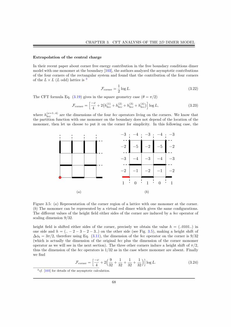
CHAPTER 3. CFT ANALYSIS OF THE 2D DIMER MODEL
Extrapolation of the central charge
In their recent paper about corner free energy contribution in the free boundary conditions dimermodel with one monomer at the boundary [103], the authors analyzed the asymptotic contributionsof the four corners of the rectangular system and found that the contribution of the four cornersof the L× L (L odd) lattice is 3
Fcorner =1
2logL. (3.22)
The CFT formula Eq. (3.19) gives in the square geometry case (θ = π/2)
Fcorner =[−c
4+ 2(h
(1)bcc + h
(2)bcc + h
(3)bcc + h
(4)bcc
)]logL, (3.23)
where h(ν=1..4)bcc are the dimensions of the four bcc operators living on the corners. We know that
the partition function with one monomer on the boundary does not depend of the location of themonomer, then let us choose to put it on the corner for simplicity. In this following case, the
1 0 1 0 1
−2 −1 −2 −1 −2
−3 −4 −3 −4 −3
−2 −5 −2 −5 −2
−3 −4 −3 −4 −3
(a) (b)
Figure 3.5: (a) Representation of the corner region of a lattice with one monomer at the corner.(b) The monomer can be represented by a virtual red dimer which gives the same configurations.The different values of the height field either sides of the corner are induced by a bcc operator ofscaling dimension 9/32.
height field is shifted either sides of the corner, precisely we obtain the value h = (..0101..) inone side and h = (.. − 2 − 3 − 2 − 3..) on the other side (see Fig. 3.5), making a height shift of∆φb = 3π/2, therefore using Eq. (3.11), the dimension of the bcc operator on the corner is 9/32(which is actually the dimension of the original bcc plus the dimension of the corner monomeroperator as we will see in the next section). The three other corners induce a height shift of π/2,thus the dimension of the bcc operators is 1/32 as in the case where monomer are absent. Finallywe find
Fcorner =[−c
4+ 2( 9
32+
1
32+
1
32+
1
32
)]logL. (3.24)
3cf. [103] for details of the asymptotic calculation.
68
CHAPTER 3. CFT ANALYSIS OF THE 2D DIMER MODEL
The comparison with the asymptotic result Eq. (3.22) gives us the value of the central charge ofthe free bosonic field theory, i.e. c = 1. One can notice that the same result holds if the monomeris somewhere on the boundary but not at the corner, in that case, there is five bcc operrtors, four oneach corners of dimension 1/32 and another responsible for the shift at the surface with dimension1/2 then using Eq. (3.19)
Fcorner =[−c
4+
1
2+ 2( 1
32+
1
32+
1
32+
1
32
)]logL =
1
2logL, (3.25)
in accordance with the fact that the partition function with one boundary monomer does notdepend of its location. Obviously this result seems completely natural in the height mappingframework or in the free complex fermion representation of the dimer model Eq. (5.9), nonethelessthe presence of bcc operators acting on the corners has never been extensively studied in thiscontext, leading to misinterpretation of asymptotic results and thus to a different value of thecentral charge of the theory. In the pure dimer situation Eq. (5.2), the four bcc operators hasdimension 1/32, we claim that the corner free energy should be equal to
Fcorner =[−1
4+ 2(4hbcc
)]logL = 0. (3.26)
This result nicely agrees with the literature, where no corner free energy term has never beenfound in the free boundary conditions close packed dimer model, neither theoretically [29] nornumerically [136], strengthening our analysis. Obviously the number of monomers does not playany role at the thermodynamic limit because the density is always zero. The result depends onlyon the parity of the lattice and the analysis of the model with zero and one monomer are just thesimplest cases that we can study leading to the general statement
• Fcorner = 0 for an even lattice.
• Fcorner = 1/2 logL for an odd lattice.
We claim here that the analysis of the free energy in the height mapping formulation of boundaryconditions, leads again to c = 1. In the following section, we shall compute analytically correlationfunctions between monomers where boundary fields has to be properly interpreted and we willshow that the exact solution fully agrees with this theory, reinforcing the present result aboutthe significance of these bcc operators. Finally we conclude, that the free bosonic formulation ofthe dimer model allows for the complete study and interpretation of finite size effects in a CFTcontext, and unified all the results known about this very simple but non-trivial model.
A word about the c = −2 CFT
It is beyond the scope of this thesis to enter into the wide area of conformal analysis of finite sizeeffects (see [194] for more details), nor all the literature of c = −2 models, but just to pointingout the difference of result when one looks carefully at the bcc operator contribution in the cornerfree energy. This statement is also based on the mapping of the dimer model to the spanning treemodel [200] and, equivalently, to the Abelian sandpile model [152] which both belong to a c = −2symplectic fermion theory. Taking hbcc = 0 leads de facto to c = −2, suggesting that the dimermodel may be a logarithmic CFT (LCFT) [106, 178, 182]. This argument turns out to be valid in
69

CHAPTER 3. CFT ANALYSIS OF THE 2D DIMER MODEL
Figure 3.6: A dimer configuration on the square lattice with open boundary condition on the leftand its equivalent spanning tree representation as explained in the first chapter. Here there is twokind of boundary conditions for the tree, open on the top and right and closed on the left andbottom, which can be tacking into account using two bcc operators of dimension -1/8. Figuresfrom [106]
the spanning trees formulation because in the odd case, there is no change of boundary conditionsat the corners while in the even geometry, there is two bcc of dimensions -1/8 on opposite corners(see Fig. 3.6). It will be very interesting to understand in details how to reconcile the two CFTdescriptions of the dimer model, and we let this problem for futur work.
3.2.3 Transfer matrix formulation and CFT on a infinite strip
Previously another type of finite size effect analysis [106] has been performed for the close packingdimer model on a strip with periodic and free boundary conditions, and it has been shown thatthe result depends strongly on the parity of the length of the strip as it should be, and the notionof effective central charge has to be introduce [99]. We consider a square lattice with periodicboundary conditions and an even number of columns N and consider a staggered configuration.Consider now superposing a generic dimer configuration with the staggered configuration, theresulting superposition is shown in fig and consists in a certain number s of strings (see Fig. 3.7).The dynamics under which these strings propagate in the vertical direction has the followingproperties 4
• The configurations of dimer fully determine by the configurations of strings.
• The number of strings is conserved i.e. the number of fermions is conserved, so that thetransfer matrix is block-diagonal.
• When moving from a horizontal row to the next, a string can either go straight or jumpexactly one site to the left or to the right.
4More details about the transfer matrix can be found in the next chapter
70

CHAPTER 3. CFT ANALYSIS OF THE 2D DIMER MODEL
These properties follow directly from the definition of the superposition and from the definition ofa valid dimer covering. The properties of strings suggest to view dimer configurations as a discretetime evolution process, where the time increases along the vertical direction. In what follows itis convenient to refer to the horizontal direction as space and vertical direction as time. Thetime evolution is then accomplished by the row-to-row transfer matrix T which will be detailedbelow. We view the system as a set of fermionic particles on the lattice Z + 1/2 that evolve inthe y-direction, which is imaginary time. We do not write down explicitly the actual form of the
Figure 3.7: We choose a staggered dimer configuration which we call a reference configuration(red). Any other dimer configuration (blue) will be compared to the reference by superposition ofthe two. We define the particle locations as the vertical edges that are not occupied by a real dimeronly a reference one. Particles can jump from a vertical edge to another only if a real horizontaldimer connects the two. Here, a fermion will be defined as an even vertical edge occupied only bya reference dimer or an odd vertical edge occupied only by a real dimer.
transfer matrix here, since we dot not need its expression for the purpose of the discussion and willbe fully detailed in the next chapter about the arctic circle phenomenon. The partition functionfor periodic boundary conditions in the imaginary-time direction is
Q0 = TrTN . (3.27)
Through this expression, the analogy between a quantum 1d model and a 2d statistical system isobvious and will be useful to characterize the conformal spectrum of a classical or quantum theoryon a strip or cylinder. In all cases, the free energy per site can be related to the leading eigenvalueof the transfer matrix 5, and critical exponents can be inferred from various subleading eigenvalues.A powerful tool that we will use for analyzing critical properties of a model is various geometriesin the conformal mapping. Here on may ask about the form of the free energy when one chooseto consider the dimer model on a infinite long strip of width L. One obvious consequence is thatthe value of the height field on both sides of the strip will depend of the parity of L. For L eventhe two boundary values are the same while there are not for odd L (see Fig. 3.9). The half-plane
5or the exponential of the hamiltonian
71

CHAPTER 3. CFT ANALYSIS OF THE 2D DIMER MODEL
Φαβα β
iLπlog(.)
α β
L
Figure 3.8: Conformal mapping between the half-plane with a bcc operator Φαβ in 0 and the stripewith different boundary conditions on the left and right of the strip. Figure from [58]
can be mapped into a infinite stripe of width L using the following conformal mapping
w =iL
πlog z, (3.28)
which can be used to compute correlation functions in this geometry starting from correlation onthe half-plane. The general form of the free energy per unit length of an infinitely long strip offinite width L at criticality is
FL = fbulkL+ fsurf +A
L+ ..., (3.29)
where fbulk is the free energy per bulk site, and fbulk is the free energy per boundary site assumingidentical boundary conditions on the two sides of the strip, and A is a constant. Unlike thefree energy densities fbulk and fsurf , the constant A is universal. The value of A is related to thecentral charge c of the underlying CFT, and depends on the boundary conditions in the transversaldirection. This last point will be crucial here, indeed in the case or dimer model on a strip theboundary conditions on both side of the strip will depend on the parity of the width L. Thesedifferent boundary conditions in the strip geometry will lead to a change of boundary condition inthe point x = 0 of the real line in the half space geometry (see Fig. 3.8). This change of boundarycondition will be interpreted, just like in the case of the corner we saw before, as the presence ofa bcc operator acting on the boundary. This bcc has to be carefully analyzed and its conformaldimension will appear in the expression of the universal part of the free energy. The details of thecalculation are not presenting here since there are quite standard and we send the curious readerto [21, 39, 38] for details.
Cylinder geometry
In the cylinder geometry the actual expression for the constant term A(cyl) is
A(cyl) = − π
24ceff = 4π
(hbcc −
c
24
), (3.30)
72
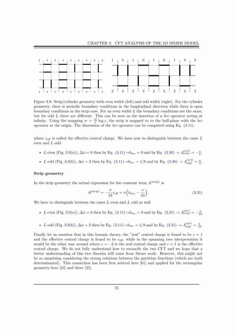
CHAPTER 3. CFT ANALYSIS OF THE 2D DIMER MODEL
2 3 2 3 2 3 2 3 2
2 3 2 3 2 3 2 3 2
2 3 2 3 2 3 2 3 2
1 0 1 0 1 0 1 0 0
Figure 3.9: Strip/cylinder geometry with even width (left) and odd width (right). For the cylindergeometry, there is periodic boundary conditions in the longitudinal direction while there is openboundary conditions in the strip case. For an even width L the boundary conditions are the same,but for odd L there are different. This can be seen as the insertion of a bcc operator acting atinfinity. Using the mapping w = iL
π log z, the strip is mapped to to the half-plane with the bccoperator at the origin. The dimension of the bcc operator can be computed using Eq. (3.11).
where ceff is called the effective central charge. We have now to distinguish between the cases Leven and L odd
• L even (Fig. 3.9(a)), ∆φ = 0 then by Eq. (3.11)→hbcc = 0 and by Eq. (3.30)→ A(cyl)even = −π6 .
• L odd (Fig. 3.9(b)), ∆φ = 2 then by Eq. (3.11)→hbcc = 1/8 and by Eq. (3.30)→ A(cyl)odd = π
3 .
Strip geometry
In the strip geometry the actual expression for the constant term A(strip) is
A(strip) = − π
24ceff = π
(hbcc −
c
24
). (3.31)
We have to distinguish between the cases L even and L odd as well
• L even (Fig. 3.9(a)), ∆φ = 0 then by Eq. (3.11)→hbcc = 0 and by Eq. (3.31)→ A(str)even = − π
24.
• L odd (Fig. 3.9(b)), ∆φ = 2 then by Eq. (3.11)→hbcc = 1/8 and by Eq. (3.31)→ A(str)odd = π
12 .
Finally let us mention that in this bosonic theory, the ”real” central charge is found to be c = 1and the effective central charge is found to be ceff , while in the spanning tree interpretation itwould be the other way around where c = −2 is the real central charge and c = 1 is the effectivecentral charge. We do not fully understand how to reconcile the two CFT and we hope that abetter understanding of this two theories will come from future work. However, this might notbe so surprising considering the strong relations between the partition functions (which are bothdeterminantal). This connection has been first noticed here [61] and applied for the rectangulargeometry here [24] and there [25].
73

CHAPTER 3. CFT ANALYSIS OF THE 2D DIMER MODEL
3.3 Scaling behavior of monomer and dimer correlation
functions
3.3.1 Boundary conformal dimensions
After the study in full details of the expression of the free energy in the rectangular and strip (andcylinder) geometries, the next step will be to determined all the correlations in the model, albeittheir scaling dimension and amplitudes. If we take, for a moment, the example of the Ising modelfrom a CFT point a view. We know that the conformal content is fairly simple, i.e. that onlytwo operators are primary (actually three with the unity operator), which are the spin operatorσ and the energy density operator ǫ. In this unitary CFT, we know from the Kac table that
hσ = hσ := x(σ)b = 1/16 and hǫ = hǫ = x
(ǫ)b = 1/2. These scaling dimensions are valid in the
bulk, specified by the index b. In 2d any analytical function w(z) on the complex plane providesa conformal mapping with a local dilation factor b(z) = |dz/dw|. Such mapping can be used todeduce surface exponents starting from the half-space geometry. The same conformal mappingapproach can be used to extract exponents close to a wedge of angle θ, is that case the surfaceexponent is recover in the limit θ → π. The corner and surface exponents are not independent andand relation can be found between them using conformal invariance (see box 8 below)
In two dimensions the critical behavior near a wedge can be related to that of a half-plane if the system shows conformal invariance. Consider the conformal transformationw = zθ/π, which maps the surface geometry of the z-plane into a wedge of opening angleθ in the w-plane. If one knows the dimension of an operator on the surface xs, it ispossible to compute the scaling dimension of the same close to a wedge of internal angleθ using this transformation, and the result is
xc =π
θxs, (3.32)
which for θ = π/2 give xc = 2xs. The details of this calculation can be found in the nicereview [96] where all kinds of geometries are studied thoroughly.
Box 8 (Corner dimension).
Conformal invariance predicts more than just exponents of correlation functions, but also predictsthe complete form of the correlation functions, and how the correlators scale with the distance tothe surface of corner. In the following, we will be interesting only on the exponents for dimer andmonomer correlations and the full analysis of the correlations are not presented here.
3.3.2 Monomer correlations
Here, we shall analyze monomer-monomer correlation functions using our pfaffian solution detailedpreviously and compared to the Coulomb gas interpretation of the dimer model. As we saw inthe previous section, the dimer model on a rectangular geometry admits bcc operators on every
74

CHAPTER 3. CFT ANALYSIS OF THE 2D DIMER MODEL
of the four corners, and it has to be taken into account for the analysis of the scaling dimensionoperators, in particular for corner correlations. Indeed in the case of monomers deep in the bulk6
or deep in the surface7, the scaling dimensions are respectively x(m)b = 1/4 and x
(m)s = 1/2, leading
to the following scaling of correlation functions (see Fig. 3.11(a))
monomer correlations→
bulk-bulk behavior→ C(L) ∼ L−2x(m)
b ∼ L−1/2
surface-surface behavior→ C(L) ∼ L−2x(m)s ∼ L−1
bulk-surface behavior→ C(L) ∼ L−x(m)s −x
(m)
b ∼ L−3/4.
(3.33)
These known results are in perfect agreement with our exact solution (cf. Fig. 3.10) where we fixedthe positions of two monomers for increasing system size L (all the correlations are measured fortx = ty = 1).
The amplitude B of the asymptotic two-point correlation function, which behaves likeBd−1/2, has been determined explicitly in the thermodynamic limit [13], B = 2−3/4A2 ≈0.247... with A = 21/12e3ζ′(−1) and where ζ(s) is the Riemann zeta function. This valueappears to be in perfect agreement with our numerical fit. Our exact solution allows fornumerical extrapolation of amplitudes for any monomer (and also dimer) correlationswith a very high precision.
Box 9 (Amplitudes of the monomer correlations).
10 5020 3015
5�10�4
0.001
0.005
0.010
0.050
L−1
L−1/2
C(L
)
L60. 65. 70. 75. 80.
0.028
0.029
0.03
0.031
0.032
0.033
0.034
0.035
L−3/4
C(L
)
L
(a) (b)
Figure 3.10: (a) Bulk-bulk and surface-surface correlation functions. (b) Bulk-surface monomercorrelation functions
The behaviors of bulk and surface monomer correlation functions had already been studied inseveral papers, and the scaling dimensions are related to the scaling dimensions of operators of the2d Ising model via the expression of monomer-monomer correlations as spin-spin correlations [13].
6far from surfaces and corners.7far from corners.
75

CHAPTER 3. CFT ANALYSIS OF THE 2D DIMER MODEL
Corner critical behavior
Now we consider the effects of corners in our system, which seems to be more difficult to consideras we have seen for the corner contribution to the free energy. Fortunately conformal invariancepredicts a relation for the scaling dimension of an operator in the vicinity of a corner of an angleθ in terms of the scaling dimension of the same operator on the surface [39]
xc =π
θxs. (3.34)
If we believe in this formula, we should obtain the value x(m)c = 1 for θ = π/2, which leads to the
behavior C(L) ∼ L−2 for corner-corner correlation functions. This result contradicts our exactevaluation, where the exponent seems to change according to the exact location of the monomers(see Fig. 3.11(b) and Fig. 3.13), and where three different cases arise. Unlike the surface and bulkcases where the scaling dimensions are uniquely defined, the corner scaling dimension appears tobe less trivial to analyze, and the influence of the bcc operators has to be carefully taking intoaccount. We should mention that the same kind of analysis has been done for the Ising model,where the magnetization was measured for various spins close to a corner [169]. We saw previously
(a) (b)
x(m,d)b
x(m,d)c x
(m,d)s
Figure 3.11: (a) Bulk, surface and corner decomposition of the square. (b) Representation of thevalues of the scaling dimensions of monomer operators close to the corners. Monomers on red sites
have dimension x(m)c+ = 1/2 while monomers on green sites have dimension x
(m)c− = 3/2. Let us
notice that this distinction is different from the even/odd sublattice distinction because oppositesublattice sites may have the same dimension and vice verca.
Eq. (3.23), that bcc operators add a logarithm term in the expression of the free energy F of arectangular system, then this contribution to the partition function scale as
Q(L) ∼ L−2(h
(1)
bcc+h
(2)
bcc+h
(3)
bcc+h
(4)
bcc
)= L−2(1/32+1/32+1/32+1/32). (3.35)
Indeed putting two monomers exactly on the corner of the same boundary (see Fig. 3.13(a)) isequivalent to a height shift of value 3π/2 in each corner. This height shift is induced by an
76

CHAPTER 3. CFT ANALYSIS OF THE 2D DIMER MODEL
operator of dimension 9/32, leading to the following behavior of the partition function with thetwo monomers
Q2(L) ∼ L−2(
1/32+1/32+9/32+9/32). (3.36)
Here the correlation function scale then as C(L) = Q2Q−10 ∼ L−1 leading to the value x
(m)c = 1/2
of the monomer corner scaling dimension. Nevertheless, if one choose the diagonal corners (seeFig. 3.13(b)), we place a monomer on the first corner which is again equivalent to the insertionof a bcc operator of dimension 9/32 (see Fig. 3.5) and the other one on a neighboring site ofthe other corner which is equivalent to the insertion of a bcc operator of dimension 25/32 (seeFig. 3.12), we found the behavior C(L) ∼ L−2. Finally, if both of the two monomers are on a
0 1 4 5 4
−1 2 3 2 3
0 1 0 1 0
−1 −2 −1 −2 −1
0 1 0 1 0
(a) (b)
Figure 3.12: (a) Representation of the corner region of a lattice with one monomer at the corner.(b) The monomer can be represented by a virtual red dimer which gives the same configurations.The different values of the height field either sides of the corner are induced by a bcc operator ofscaling dimension 25/32.
neighboring site of a corner (see Fig. 3.13(c)), then the correlation function is C(L) ∼ L−3. Thisthree different situations are summarized in Fig. 3.13, showing that our exact computations are inperfect agreements with Coulomb gas predictions for the behavior of correlation functions in thevicinity of a corner. A more general statement is that the monomer scaling dimension near a cornerdepends crucially of the sublattice considered as explained in Fig. 3.11(b). This phenomena leads to
two different values of the scaling dimensions of corner monomers x(m)c+ = 1/2 and x
(m)c− = 3/2 which
is in agreement with the CFT formula Eq. (3.34) in average x(m)c = (x
(m)c+ + x
(m)c− )/2 = 2x
(m)s = 1
when lattice effects are forgotten.
Finite size scaling
A general study of the finite size behavior of correlation functions can be performed as well, leadingto the following scaling ansatz
C(r1, r2, L) = |r1 − r2|−x1−x2Φ(|r1 − r2|−1L), (3.37)
77
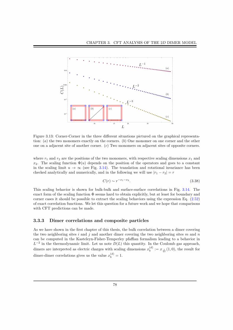
CHAPTER 3. CFT ANALYSIS OF THE 2D DIMER MODEL
10 5020 3015
10�5
10�4
0.001
0.01
L−2
L−3
L−1C(L
)
L
(b)(a) (c)
(a)
(b)
(c)
Figure 3.13: Corner-Corner in the three different situations pictured on the graphical representa-tion: (a) the two monomers exactly on the corners. (b) One monomer on one corner and the otherone on a adjacent site of another corner. (c) Two monomers on adjacent sites of opposite corners.
where r1 and r2 are the positions of the two monomers, with respective scaling dimensions x1 andx2. The scaling function Φ(u) depends on the position of the operators and goes to a constantin the scaling limit u → ∞ (see Fig. 3.14). The translation and rotational invariance has beenchecked analytically and numerically, and in the following we will use |r1 − r2| = r
C(r) ∼ r−x1−x2 . (3.38)
This scaling behavior is shown for bulk-bulk and surface-surface correlations in Fig. 3.14. Theexact form of the scaling function Φ seems hard to obtain explicitly, but at least for boundary andcorner cases it should be possible to extract the scaling behaviors using the expression Eq. (2.52)of exact correlation functions. We let this question for a future work and we hope that comparisonswith CFT predictions can be made.
3.3.3 Dimer correlations and composite particles
As we have shown in the first chapter of this thesis, the bulk correlation between a dimer coveringthe two neighboring sites i and j and another dimer covering the two neighboring sites m and ncan be computed in the Kasteleyn-Fisher-Temperley pfaffian formalism leading to a behavior inL−2 in the thermodynamic limit. Let us note D(L) this quantity. In the Coulomb gas approach,
dimers are interpreted as electric charges with scaling dimensions x(d)b := x 1
4π(1, 0), the result for
dimer-dimer correlations gives us the value x(d)b = 1.
78

CHAPTER 3. CFT ANALYSIS OF THE 2D DIMER MODEL
1.0 2.0 3.01.5
2.0
1.5
5.03.0
0.9
0.95
1.
1.05
1.1
1.15
r1/2C(r,L
)
rC(r,L
)
L/r
L/r
Figure 3.14: Finite size scaling of monomer surface-surface and bulk-bulk (inset) correlation func-tions in log-log scale for L = 100, 200, 300, 400. The surface correlations are measured far from thecorners and the bulk correlations are measured far from boundaries and corners.
Dimer correlations
Actually it is straightforward to study dimer correlations here. Indeed a dimer can be seen astwo neighboring monomers, thus a dimer-dimer correlation is simply a 4-point monomer-monomercorrelation, which can be evaluated with our solution. In the following, one shows how to constructthe dimer-dimer correlation in the boundary case, for the bulk case the situation is essentially thesame but expressions are less convenient. Explicitly the correlation between two dimers at position(ri, rj) and (rm, rn) is
Q4(ri, rj , rm, rn)Q−10 = CijCmn − CimCjn + CinCjm. (3.39)
If we choose that ri and rm are on the same sublattice (then rj and rn are on the other one),a straightforward consequence is that the second term CimCjn vanishes, moreover the first termCijCmn tends to a constant in the thermodynamic limit in such way that we can define the dimer-dimer correlation function as
Q4(ri, rj , rm, rn)Q−10 − CijCmn = CinCjm ∼ D(L). (3.40)
In this way, all the configurations of dimer correlations are available, and all the scaling dimensionsof electric charges (bulk, surface, corner) may be analyzed stricto sensu and compared with theCoulomb gas theory. We can show that the well known bulk behavior is recovered very precisely,furthermore, surface and corner correlations may be examined as well leading to the followingbehaviors
dimer correlations→
bulk-bulk behavior → D(L) ∼ L−2x(d)
b ∼ L−2,
surface-surface behavior→ D(L) ∼ L−2x(d)s ∼ L−2,
corner-corner behavior→ D(L) ∼ L−2x(d)c ∼ L−4.
(3.41)
79

CHAPTER 3. CFT ANALYSIS OF THE 2D DIMER MODEL
Unlike monomer correlations, dimer correlations are much easier to interpret in the Coulomb gasframework. Indeed, the absence of additional change of boundary conditions8 in the partitionfunction allows for a direct determination of dimer scaling dimensions. The particular form of
scaling dimension (gfree = 1/4π) bulk surface corner
x(d) 1 1 2x(m) 1/4 1/2 1/2 or 3/2
Table 3.1: Bulk, surface and corner values of dimer and monomer scaling dimensions for the free(gfree = 1/4π) fixed point. The corner monomer scaling dimension depends of its exact location.
dimer correlations Eq. (3.40) predicts that x(d)s = 2x
(m)s = 19 and x
(d)c = x
(m)c+ + x
(m)c− = 210. We
notice here that the formula Eq. (3.34) checked out in that case. A careful and detailed studyof surface and corner operators has to be performed to unravel this point. The scaling form ofcorrelation functions Eq. (3.37) holds in the dimer case as well, using the dimer scaling dimensions(see Table 3.1). The solution presented here can be also used to calculate more complex correlationfunctions, combining dimer and monomer scaling dimensions. A posteriori, more complicatedobject like trimers with dimension x•••, quadrimers with dimension x•••• or more generally, stringof k neighboring monomers (k-mer) with dimension x•...•, can be studied as well, which correspondto various charged particles in the Coulomb gas formalism.
Quantum dimer model and classical limit
Dimer models have regained interest because of its quantum version, the so-called quantum dimermodel, originally introduced by Rokhsar and Kivelson [183] in a condensed matter context. Thismodel was introduced to give a description of the phenomena of resonating valence bond states byAnderson. Consider all dimer coverings of the square lattice. To each configuration assign a vector.Assume these vectors form an orthogonal basis for the Hilbert space. Notice that if we rotate aplaquette with two parallel dimers we get an allowed configuration. These special plaquettes arecalled flippable. Let us write the Hamiltonian by introducing local kinetic and potential terms.where a dimer represent a singlet of two spins. One of the nice feature of the quantum dimer
H =∑[v
t(|� �
��
〉〈� �
��
|+ |� �
��
〉〈� �
��
|)− (|� �
��
〉〈� �
��
|+ |� �
��
〉〈� �
��
|)]
model is its relation to the classical model at the point v/t = 1 of the parameter space, namelythe so-called Rokhsar-Kivelson (RK) point. Specifically, the ground state of the wave-function atthis RK point can be written as the partition function of the classical model
|Ψ0〉RK =1√Q0
∑
C
|C〉, (3.42)
8Of course the four corner bcc’s with dimension 1/32 are still present but do not play any role in dimer-dimercorrelation functions.
9Let us notice that the fact that x(d)b
= x(d)s is a pure coincidence.
10A dimer in the corner is formed by two neighboring monomers with dimension x(m)c+
and x(m)c−
.
80

CHAPTER 3. CFT ANALYSIS OF THE 2D DIMER MODEL
where∑
C |C〉 = Q0 the number of classical dimer covering of the lattice. Thus all informationsabout the ground state at the RK point comes directly from the knowledge of the partition functionof the classical model, indeed all our analysis of the dimer model holds for the RK wave function aswell. Let us mention that the full phase diagram outside the RK point is very rich and beyond thescope of the present discussion (see [156, 79] for reviews). As a step towards the understanding ofthe finite-temperature phase diagram of the quantum dimer model, we can mention the particularlimit when kinetic terms goes to zero, which is a classical dimer model with an interaction thattends to align dimers on the same plaquette. In figure Fig. 3.15, we show a particular dimer
Figure 3.15: Dimer model with plaquette interaction
configuration with 6 aligning plaquettes, representing by the green dots. If we define the numberof green dots by N , then the partition function of this model can be written as a sum of dimerconfigurations C weighted by N i.e.
Z =∑
C
exp(−βνN ), (3.43)
where ν > 0 is the strength of the interaction. Other kind of interactions can be cooked up, forexample on can create an anti-ferromagnet order choosing ν < 0 or adding interaction that tendsto align dimers along the same line in order to create a nematic order [167]. The dimer-dimercorrelations which are critical in the non-interacting case are found to remain critical, but withcontinuously varying exponents, down to a finite temperature where the dimers order through aKosterlitz-Thouless (KT) transition, we do not enter into all this details here and report the inter-ested reader to [4, 3, 55]. We mention here that the height mapping remains valid for the interactingdimer model and it can be showed that, at the critical point, the interactions renormalize the freetheory to another value of the stiffness constant g11. It has been shown that the renormalized valueof the stiffness becomes gKT = 2/π instead of gfree = 1/4π for the free case. The same analysisof corner contribution to free energy as well as scaling dimensions (bulk, surface, corner) can bestudied in the interacting dimer model using the height mapping. For the corner contribution tothe free energy term, just like the free case, the result depends only on the parity of the lattice andthe analysis of the model with zero and one monomer can be studied. As an example, the cornerfree energy for the even-case lead, using Eq. (3.23) and Eq. (3.19) to Fcorner = 7/4 logL.
11In a more fancy language, we often read that the interaction deforms the compactification radius of the freeboson.
81
CHAPTER 3. CFT ANALYSIS OF THE 2D DIMER MODEL
3.4 Conclusions and perspectives
In this work the classical dimer model was discussed in great details both in a fermionic and bosonicfield theory formulation. The bosonic formulation of the model is based on the so-called heightmapping and it is well suited for phenomenological predictions about correlations between dimersand monomers in a Coulomb gas context. Then we presented a practical and complete fermionicsolution of the 2d dimer model on the square lattice with an arbitrary number of monomers.Furthermore, the Tzeng-Wu solution of the dimer model with a boundary monomer was foundto be included in our theory. Interpretations of finite size effects of the Tzeng-Wu solution in aCFT/Coulomb gas framework has been performed, and we showed that a careful examination ofboundary conditions in the model allowed us to recover the central charge of the free fermion/freeboson field theory. The exact expression of correlation functions between monomers has beenwritten in terms of the product of two pfaffians, and we gave an explicit formula for boundarycorrelations valid for the four boundaries of the rectangle. This solution has been used to computecorrelations for several configurations in order to extract bulk, surface and corner scaling dimensionsfor dimer and monomer operators. All these results were interpreted in the Coulomb gas formalism,and we showed that all the predictions of the CFT were in accordance with a c = 1 theory.
82

CHAPTER 4. FIELD THEORY FORMULATION OF THE ARCTIC CIRCLE
CHAPTER4Field theory formulation of the arctic circle
Contents
4.1 The Aztec diamond dimer model . . . . . . . . . . . . . . . . . . . . . 84
4.1.1 Introduction and generalities . . . . . . . . . . . . . . . . . . . . . . . . 84
4.1.2 Height mapping and scalar field theory . . . . . . . . . . . . . . . . . . . 86
4.1.3 Transfer matrix formulation . . . . . . . . . . . . . . . . . . . . . . . . . 89
4.2 Classical 2d systems and 1d quantum interpretation . . . . . . . . . . 91
4.2.1 6-vertex model and DWBC . . . . . . . . . . . . . . . . . . . . . . . . . 91
4.2.2 The transfer matrix . . . . . . . . . . . . . . . . . . . . . . . . . . . . . 93
4.2.3 Fermionic chain with a generic dispersion relation . . . . . . . . . . . . 95
4.3 Arctic field theory . . . . . . . . . . . . . . . . . . . . . . . . . . . . . . 102
4.3.1 Exact correlation functions . . . . . . . . . . . . . . . . . . . . . . . . . 102
4.3.2 Long-range correlations . . . . . . . . . . . . . . . . . . . . . . . . . . . 105
4.3.3 Dirac field theory in curved space . . . . . . . . . . . . . . . . . . . . . . 107
4.4 Conclusions . . . . . . . . . . . . . . . . . . . . . . . . . . . . . . . . . . 110
83
CHAPTER 4. FIELD THEORY FORMULATION OF THE ARCTIC CIRCLE
4.1 The Aztec diamond dimer model
4.1.1 Introduction and generalities
The arctic circle is the name given by Jockush, Propp & Shor to a phenomenon they discovered in1995 [113] while studying dimer coverings of the Aztec diamond [63, 65]. The phenomenon consistsin the appearance, in the thermodynamic limit, of a curve that separates two macroscopic domains,one in which the dimers appear to be frozen, meaning that one knows their exact position with aprobability that goes quickly to one in the thermodynamic limit, and another domain where thedimers fluctuate. The same phenomenon was observed in other models [47], in particular in thesix-vertex model with domain-wall boundary conditions [139, 166, 49, 50], a system that alreadypossessed a long history connected to integrability and to the evaluation of the norm of Bethe states[140, 100, 101]. In fact, the phenomenon itself appears to have been known as early as 1977, in adifferent context though: the statistics of large Young tableaux [204]. Since the late 1990s, therehas been an intense activity in this area, which lies at the frontier between physics, mathematicsand computer science. Among the many results that were collected are the limiting distribution ofdimers around the origin in the thermodynamic limit [46, 114], the fluctuations of the boundarydescribed by the Airy process [114], a general theory for dimer models [128] and the calculation ofthe corresponding arctic curves in connection with algebraic geometry [129], calculations of variouscorrelation functions [23, 162, 164], steps towards extension to interacting models [139, 50, 48] (i.e.models that cannot be mapped to free fermions; for example: the six-vertex model at ∆ 6= 0, ordimers with aligning interactions [4]), and numerical investigations (see [54] for example). Thischapter is partially based on the following paper [6].
Aztec diamond
The Aztec diamond is defined as follows. Let us consider the diamond shaped subset containing2n2 squares. This geometry is called the Aztec diamond and can be seen as a regular square latticewhere the four corners are removed. Then one considers the set of random tilings with dominosof the Aztec diamond with uniform weight. Using a connection between domino tilings and thealternating-sign matrices, the number of dominos tilling AD(n) of the Aztec diamond of size n hasbeen computed [64, 65] and a surprising result appears
AD(n) = 2n(n+1)
2 . (4.1)
For large n the Aztec diamond divides into five regions delimited by the arctic circle found originallyby Cohn, Elkies, Noam and Propp [45]. Inside the arctic circle there is a disordered region ofthe tiling. Outside this boundary the tilings forms a completely regular brick wall pattern (e.g.Fig. 5.4). From a physics point of view, the bulk phase is a massless 1 phase and the four boundaryphases are massive (with infinite mass) phases. Let us mention that generalization of the Aztecdiamond to more complicated graph can be studied as well (see [28, 26] for example), the shape ofthe arctic curve, the partition function and some others correlation functions has been computedusing a transfer matrix formalism very similar to the one we will use in the following sections.
1”Massless” is the field theory terminology, which is synonym to ”gapless” in the condensed matter terminology,which is synonym to ”disordered” in the statistical physics terminology...
84

CHAPTER 4. FIELD THEORY FORMULATION OF THE ARCTIC CIRCLE
n
t
b
Figure 4.1: Left: Aztec diamond dimer covering. For sufficiently large sizes, a particular curveseems to separate a disordered (the temperate region) region from a frozen region (the arcticregion). In this case, the curve can be showed to be a circle. Right: Every dimer configurationsof the Aztec diamond can be mapped to configurations of non-intersecting paths, fluctuations ofthe central point (red dot). The south path (the one shown on the figure) is related to the GUETracy-Widom distribution [115]. In the case of fluctuations near the tangency points (green dots),another process arises: the GUE minor process [116]. See also box 10
It is possible to draw continuous lines in the Aztec diamond of order n by adding in eachdomino a line pattern depending on its type as shown in Fig. 5.4. Let t be the horizontalcoordinate with t = 0 in the middle of the diamond and denote bl,n(t), l = 0, ..., n − 1be the position of the lth line at time t. Then it is proven (see [115]) that, under properrescaling the first line (see Fig. 5.4) of the set of non-intersecting b0,n(0)/n1/3 → ζ2 asn→∞ with ζ2 a random variable in the gaussian unitary ensemble (GUE) distribution.This model is closely related to the corner growth process for which fluctuations can bealso computed and showed to be GUE as well. When the disordered region touches theboundaries (the tangency points) we expect that the GUE minor process should be theuniversal limit [116]. Random matrix connection has been found to appear in other limitshape phenomena, like in the 6-vertex model [51] or plane partitions [163, 164]. We willget back to boundary fluctuations later on in the fermionic transfer matrix formulation ofthe problem where the Airy kernel will show up using the exact expressions of correlatorsof fermions near the boundaries. We send the reader to one of the appendix of [6] formore details.
Box 10 (Relation to random matrix ensembles).
85

CHAPTER 4. FIELD THEORY FORMULATION OF THE ARCTIC CIRCLE
4.1.2 Height mapping and scalar field theory
In this paragraph, we shall use the same formulation of the dimer covering we have done before forthe square geometry but for the Aztec diamond. Previously we claimed that the perfect matchingof a graph G can be computed as the pfaffian of a matrix as long as the graph is planar. In thepresent case, we are dealing with the so-called Aztec diamond which can be think as a regularsquare lattice with some vertices removed. The Kasteleyn theorem can be applied for this lattice,exactly on the same way as for the usual square lattice and the Kasteleyn matrix can be writtendown explicitly without too much trouble. The main feature we want to explore in this chapteris the behavior of correlation in the scaling limit where the lattice spacing goes to zero. From apurely technical point a view, this task is rather complicated and the explicit form of the inverseKasteleyn matrix was computed by Helfgott [91]. The formula is expressed in terms of Krawtchoukpolynomials and a asymptotic analysis seems quite non-trivial.
Height field and main hypothesis
For this particular lattice, we can perform the same height mapping (see Fig. 4.2) as for the regularsquare lattice on the rectangle as we did in the previous chapter. By fixing the rescaled height
0
2 3 2
4 5 4 5 4
6 67 7 6 3 6
8 9 8 5 8 5 4 5 8
6 7 6 7 6 3 6
4 5 4 5 4
2 3 2
0
Figure 4.2: Aztec diamond dimer covering. Conversely to the rectangle geometry of the previouschapter, the boundary value of the height field is no more asymptotically flat but linear on eachedge of the diamond. The machinery of boundary CFT fails to give any information about criticalproperties of the renormalized field theory.
at an arbitrary point, e.g. h(0) = 0 on the bottom plaquette, these rules define the entire heightfunction h(~r) uniquely, exactly in the same way that for the regular square lattice we saw in thepast chapter. The next step is the assumption that the fluctuation of the height field can stillbe described by a gaussian free field in the asymptotic limit. It has been conjectured by Propp,(see [180]), that in the limit n → ∞, a random dimer tiling of the Aztec diamond looks like a
86

CHAPTER 4. FIELD THEORY FORMULATION OF THE ARCTIC CIRCLE
random dimer configuration of the usual plane under a certain measure. By integrating out theshort distance fluctuations, one obtains an effective quadratic action S0 for the bulk height fieldφ(~r) = π
2h(~r), defined in the continuum, which corresponds to the long-wavelength modes
S0[φ] ∝∫
d2x ηµν(∂µφ)(∂νφ), (4.2)
where ηµν is the flat metric. In the later case, we focused on the value of the height function atthe boundaries and found out that the asymptotic value of the field φb tends to a constant thatwe can associate to a conformal boundary field.
For any metric on a two dimensional manifold, a particular coordinate system existswhere the metric is conformally flat, i.e. the metric is the product of a scalar field (theconformal factor ξ below), with a flat metric. The components of the metric in onecoordinate system (x, y) is related to metric in a second coordinate system (w, z) by
gµν dxµ dxν = gxx dx2 + 2gxy dxdy + gyy dy2
= ξ(dw2 ± dz2).
Thus, we look for w(x, y) and z(x, y) such that gwz = 0 and gzz ± gww = 0. After atedious calculation one shows that the first equality is satisfied if
∂xw = p(gxy∂xz + gyy∂yz
)
∂yw = −p(gxx∂xz + gxy∂yz
),
and to satisfy gzz ± gww = 0 we require that
±p2 =(gxxgyy − (gxy)2
)−1= detg,
which gives ∂xw =√ggyα∂αz and ∂yw = −√ggxα∂αz which imply
∂y(√ggyα∂αz) = −∂x(
√ggxα∂αz), (4.3)
or ∇α∇αz = 0. Thus any solution of the Laplace equation on the surface, in the originalcoordinates, provides a coordinate transformation to a metric of the form gµν = ξ(dw2±dz2) with the conformal factor ξ given ξ−1 = ∇αz∇αz.
Box 11 (Conformal transformation of the metric in d = 2).
The hypothesis that the bulk field can be described by a free field plus the knowledge of boundarystates allowed us to use the machinery of boundary CFT to get informations about the scaling limitof the field φb. Here the things are rather different, indeed the bulk field can be shown to convergealso towards a free field but the boundary value of the height field is no more asymptotically flatbut linear on each edge. This boundary field does not map directly to a conformal boundaryfield because it is straightforward to show that the stress-energy tensor does not vanish on theboundaries. The simplest scenario would be that the action still describe the low energy fluctuating
87

CHAPTER 4. FIELD THEORY FORMULATION OF THE ARCTIC CIRCLE
degrees of freedom can be seen as a field-theory in a curved space-time where the flat metric isreplace by a conformal metric ηµν → gµν = e2σηµν (some basic notions of curved field theory in 2dare recall in the box 11). In this next few lines, one recall some simple notion of 2d geometry andquantum field theory that will be useful in the context of our theory. Let us consider a 2d manifoldwith a Riemann metric described by the metric tensor gµν(x) which is supposed positive2 definiteso that in any coordinate system x = xµ the interval
dx2 = gµν(x) dxµ dxν , (4.4)
is positive. The field theory is required to be generally covariant, i.e., the action functional, whichinvolves the metric g as the functional parameter. Let us consider the scalar free case (with nogauge field) where the action S0[φ(x), g(x)] must be invariant in any coordinate systems and canbe written in the following form
S0[φ(x), g(x)] =κ
2
∫d2x√g(gµν∂µφ∂νφ) (4.5)
where we have changed the notation for the stiffness constant from g to κ to avoid confusionwith the metric. The stress-energy tensor can be defined as before as the variation of the actionδS0[φ(x), g(x)] under a variation of the metric δgµν(x) → gµν(x) + δgµν(x). In 2d, things areconsiderably simpler, indeed any surface in two-dimension is conformally flat (see [60] for a surveyand the box 11 above for a short demonstration), it means that any 2d metric can be put in theform
gµν(x) = e2σ(x)ηµν , (4.6)
where ηµν is the flat metric and σ(x) is related to the scalar curvature as
R(x) = −e−2σ∂2µσ. (4.7)
The consequence of this result is that, in 2d the curved metric can be, up to a local rescaling, turnto the flat metric. Let us notice that another parameter can vary in this theory, the gauge field Aµassociate with the U(1) gauge invariance of Eq. (4.8). In that case the derivative will be replaceby a covariant derivative ∂µ → Dµ = ∂µ − iAµ. The scalar lagrangian we are looking for is thenfully determined by two functions
• the conformal factor σ(x) such that gµν = e2σηµν ,
• the gauge field Aµ such that → Dµ = ∂µ − iAµ,
and the action describing the fluctuating field inside the arctic circle may be written in a fullycovariant form as
S0[φ] ∝∫ √
g d2x gµν(Dµφ)(Dνφ). (4.8)
A more thorough discussion of the bosonic field theory inside the arctic circle will be exposedelsewhere [6]. A possible way to check if that theory describes the large scale fluctuations inside
2and non-degenerate
88

CHAPTER 4. FIELD THEORY FORMULATION OF THE ARCTIC CIRCLE
the arctic circle would be to exploit some exact results for the inverse Kasteleyn on the Aztecdiamond, and determine the asymptotic behavior of correlations anywhere inside the diamond.But as we said earlier, this task seems quite non-trivial and another approach will be used in thefollowing. Although in the next chapter we will follow another strategy and sick for the fermionizedtheory describing this c = 1 field theory, i.e. the Dirac field in curved space. For the fermionic case(the Dirac action), it is a little bit more complicated because of the Dirac matrices which satisfy{γµ, γν} = 2gµν = 2e2σ(x)ηµν , which is no more conventional Clifford algebra. We shall see laterthat this complication can be dealt with using tetrads defined as gµν = eµae
νbηab will help express
everything in the euclidian metric ηab.
4.1.3 Transfer matrix formulation
In this section, the method introduced in chapter III is applied to the dimer model on the squarelattice, where the arctic circle phenomenon has been originally discovered. We will consider thesimplest version of the dimer model where the vertical and horizontal dimers have the same Boltz-mann weight choose to unity. In that way, the computation of the partition function is nothingbut counting the perfect matching number of the square graph. The fermionic transfer matrix isformulated and diagonalized. We consider a square lattice with periodic boundary conditions andan even number of columns N and consider a staggered configuration. Consider now superposing ageneric dimer configuration with the staggered configuration, the resulting superposition is shownin Fig. 4.3 and consists in a certain number of strings propagating in the vertical direction. Thedynamic of these lines has the following properties
• The configurations of dimer fully determine by the configurations of strings.
• The number of strings is conserved i.e. the number of fermions is conserved, so that thetransfer matrix is block-diagonal.
• When moving from one horizontal row to the next, a string can either go straight or jumpexactly one site to the left or to the right.
These properties follow directly from the definition of the superposition and from the definition ofa valid dimer covering. The properties of strings suggest to view dimer configurations as a discretetime evolution process, where the time increases along the vertical direction. In what follows itis convenient to refer to the horizontal (resp. vertical) direction as space (resp. time). The timeevolution is then accomplished by the row-to-row transfer matrix T which will be detailed below.We view the system as a set of fermionic particles on the lattice Z + 1/2 that evolve in the y-direction, which is imaginary time. Here we write the transfer matrix for the dimer model on thesquare lattice. First, we are still dealing with fermionic particles on the lattice Z+ 1
2 , and with theinitial and final states |ψ0〉. The transfer matrix, however, is not invariant under translations ofone site, but only of two sites. It is convenient to distinguish the two species of fermions associatedto each sublattice
a†j ≡ c†
2j+ 12
b†j ≡ c†
2j− 12
, j ∈ Z . (4.9)
and define the even Teven transfer matrix as operators which act on the two fermions a†j and b†
j as
Teven a†j T
−1even = a†
j ,
Teven b†j T
−1even = a†
j−1 + b†j + a†
j . (4.10)
89

CHAPTER 4. FIELD THEORY FORMULATION OF THE ARCTIC CIRCLE
Teven
Todd
Teven
Todd
Teven
Todd
a†i+1b†i+1a†ib†ia†i−1b†i−1
CFT
Disordered region
Figure 4.3: Left: We define the particle locations as the vertical edges that are not occupied by areal dimer only a reference one. Particles can jump from a vertical edge to another only if a realhorizontal dimer connects the two. This superposition consists in a certain number of strings. Itcan go to the left, straight ahead, or to the right. In this setup. Right: The Aztec diamond caneasily be generated by imposing a particular configuration of dimer at the bottom and bottom ofthe lattice (red dimers), in such way that this condition freezes every dimers in a certain region(blue dimers). In terms of fermion, the initial and final states |Ψ0〉 are the so-called domain wallinitial states that we will define precisely in the main text.
and the odd transfer matrix and odd Todd which act as
Todd a†j T
−1odd = b†
j+1 + a†j + b†
j ,
Todd b†j T
−1odd = b†
j . (4.11)
The Fourier modes are defined as
a†(k) =∑
j∈Z
eikj a†(j) b†(k) =∑
j∈Z
eikj b†(j) , k ∈ [−π, π] , (4.12)
in such way that the even and odd transfer matrices read in Fourier space
Teven
(a†(k)
b†(k)
)T−1
even =
(1 0
1 + eik 1
)(a†(k)
b†(k)
)
Todd
(a†(k)
b†(k)
)T−1
odd =
(1 1 + e−ik
0 1
)(a†(k)
b†(k)
) (4.13)
In terms of the fermions a and b the initial state |Ψ0〉 can be defined as a state filled (empty) offermions b (of fermions a) on one side and empty (filled) on the right. Now, let us consider the
90

CHAPTER 4. FIELD THEORY FORMULATION OF THE ARCTIC CIRCLE
double-row transfer matrix T 2 = TevenTodd,
T 2
(a†(k)
b†(k)
)T−2 =
1 2e−ik/2 cos k2
2eik/2 cos k2 1 + 4 cos2 k2
(a†(k)
b†(k)
). (4.14)
T 2 is hermitian, and it is easily diagonalized
T 2 = exp
[−∫
dk
2π2ε(k)
(c†
+(k)c+(k)− c†−(k)c−(k)
)](4.15)
with(c†
+(k)
c†−(k)
)= U(k)
(a†(k)
b†(k)
)=
(sinα(k) e−ik/2 cosα(k)
cosα(k) −e−ik/2 sinα(k)
)(a†(k)
b†(k)
)(4.16)
and
ε(k) = − log λ = −arcsinh
(cos
k
2
)(4.17)
λ(k) = tanα(k) =
√1 + cos2
k
2− cos
k
2. (4.18)
From this point of view, the analogy with 1d quantum spin chain is obvious. The double-rowtransfer matrix T 2 can be seen as the exponential of a quantum hamiltonian for the two kind offermions c+ and c−. The two crucial ingredients (see Fig. 4.3) are now the free-fermion hamiltonianH = − log T 2 and the DWIS |ψ0〉 which can be defined in the basis {c+, c−}. In the next section,we shall see that the exact same analogy can be done for the 6-vertex model that we will interpretedas a 1d quantum problem with particular initial and final state.
4.2 Classical 2d systems and 1d quantum interpretation
In the past section we have seen how one can interpreted the arctic circle phenomenon in thedimer model in terms of the evolution of a 1d fermionic hamiltonian with particular initial andfinal states. The problem of computation of local observables in the arctic circle is equivalent to thecomputation of observables in the quantum quench protocol. Another typical model for which thephenomenon of arctic curve is very much studied is the 6-vertex model with domain wall boundaryconditions (DWBC) [218], where some features has been computed exactly (see [9, 49, 50, 51] fordetails and references) for any value ∆ of the model.
4.2.1 6-vertex model and DWBC
The 6-vertex model is defined in terms of local Boltzmann weights which live on the vertices of ageneral graph and is the prototypal model of an exactly solved model in statistical mechanics. For
91

CHAPTER 4. FIELD THEORY FORMULATION OF THE ARCTIC CIRCLE
a general introduction and solution of this solved model one can not avoid Baxter’s book [17]. Itis conventional to draw the vertices of the six-vertex model as
a a b b c c (4.19)
with weights a, b, c ∈ R. The configurations of the six-vertex model are in one-to-one correspon-dence with (directed) self-avoiding trajectories on the square lattice as illustrated in Fig. 4.4.(c).The trajectories can touch—a situation that corresponds to the first vertex with weight a—, butthey cannot overlap along an edge. By convention, we decide that the trajectories never cross. Thisis convenient, because then we do not have to be too careful about the statistics of the particleswhose trajectories we are describing. We view the system as a set of fermionic particles on thelattice Z+ 1
2 that evolve in the y-direction, which is imaginary time. The six vertices drawn aboveare then operators acting on two neighboring sites x and x+ 1. They can be written respectivelyas
weight a :
c†xcx c
†x+1cx+1
(1− c†xcx) (1− c†
x+1cx+1)
weight b :
c†xcx+1
c†x+1cx
weight c :
(1− c†xcx)c†
x+1cx+1
c†xcx(1− c†
x+1cx+1) .
(4.20)
Summing these six terms, we build the R-matrix of the six-vertex model,
Rx,x+1 = a[c†xcx c
†x+1cx+1 + (1− c†
xcx) (1− c†x+1cx+1)
]
+ b[c†xcx+1 + c†
x+1cx
]
+ c[c†xcx(1− c†
x+1cx+1) + (1− c†xcx)c†
x+1cx+1
], (4.21)
which can be written as
Rx,x+1 = a exp[log(b+ c
a
)(c†xcx+1 + c†
x+1cx
)],
provided that
∆ =a2 + b2 − c2
2ab= 0 , (4.22)
and this is what we assume from now on. Since theR-matrix is gaussian at ∆ = 0, the model is free,the transfer matrix is gaussian as well, and all observables can be obtained from the propagator
92

CHAPTER 4. FIELD THEORY FORMULATION OF THE ARCTIC CIRCLE
using Wick’s theorem. The techniques developed in previous parts apply, as we explain below.We focus once again on the DWIS |Ψ0〉, which is completely filled with particles on the left, andcompletely empty on the right. The evolution of the system is generated by iterations the transfermatrix. After a number of iterations, we project the one-dimensional system of particles back tothe DWIS (Fig. 4.4.(a)). Because of the initial and final states, most vertices on the left andright of the system are forced to be in the configurations with weight a in (4.19), as illustrated inFig. 4.4.(b). Only a central region, which turns out to be a square, is not determined a priori bythose initial and final states. The square in the middle hosts configurations of the six-vertex modelwith boundary conditions (Fig. 4.4.(b)) that are known traditionally as ”domain-wall boundaryconditions”. Therefore, our setup, which combines the DWIS with the transfer matrix, is wellsuited to revisit this popular problem.
x
y
(a) (b) (c)
Figure 4.4: Six-vertex model on the square lattice. We regard the horizontal axis as space, andthe vertical axis as imaginary time. (a) One starts form the domain-wall initial state (DWIS) atthe bottom, then we apply the transfer matrix several times, and finally, we project back to theDWIS at the top. (b) Because of the DWIS, a large number of edges are constrained to be eitherempty or filled; the only vertices that are not fixed by the choice of boundary conditions are theones inside the square region in the middle of the figure. This central square is what is known inthe literature as the six-vertex model with domain-wall boundary conditions. (c) A configurationof vertices compatible with the boundary conditions: note that one can interpret the filled edgesas trajectories in space-time. This is the idea of the mapping to a fermion model.
4.2.2 The transfer matrix
We need to define two transfer matrices, one for the even rows and another for the odd rows. Usingthe notations of the previous chapter, we call a†, a the fermion creation/annihilation modes that
93

CHAPTER 4. FIELD THEORY FORMULATION OF THE ARCTIC CIRCLE
live on the the sublattice 2Z + 12 , and b†, b the ones that live on 2Z− 1
2 . Then we write
Tab ≡∏
x∈2Z+ 12
Rx,x+1
Tba ≡∏
x∈2Z− 12
Rx,x+1 .(4.23)
Notice that the terms commute within each product; but, of course, TabTba 6= TbaTab. The weightedconfigurations of the model are obtained by applying iteratively these two operators one after theother. One could then focus on one of the double-row transfer matrices TabTba or TbaTab, which
0
0.2
0.4
0.6
0.8
1.0
�6�4�202460
y
x
+N
−N
0
0
0.2
0.4
0.6
0.8
1
Figure 4.5: Numerical density snapshot for a system of size 2N = 400, and for b/a = 1/2,c/a =
√1 + b2, for general parameters satisfying the free fermion condition a2 + b2 = c2 the
arctic curve is an ellipse. The shape of the arctic curve as well as the partition function has beencomputed out of the free-fermion point in [139, 218]
generate the imaginary time evolution. However the drawback of both those operators is that theyare not hermitian, it is more convenient for the following, to deal with a hermitian generator oftranslations in imaginary time. Thus, we define our (double-row) transfer matrix as the operator
T 2 = T12
ab Tba T12
ab (4.24)
whose hermiticity follows from T †ab = Tab and T †
ba = Tba. Again, the upper script/exponent in T 2
is there to remind us that it is an operator that adds two rows to the system, instead of one. Wewill always deal with T 2, there will be no object T . Now let’s diagonalize T 2. In k-space, usingthe definition (4.12), the Fourier modes are
Tab = exp[log(b+ c
a
)∫dk2π
(ei
k2 a†(k)b(k) + e−i k
2 b†(k)a(k))]
Tba = exp[log(b+ c
a
)∫dk2π
(e−i k
2 a†(k)b(k) + eik2 b†(k)a(k)
)].
(4.25)
94

CHAPTER 4. FIELD THEORY FORMULATION OF THE ARCTIC CIRCLE
Then the problem boils down to the diagonalization3 of a 2× 2 matrix
T 2 = exp[−∫ π
−π
dk2π
2ε(k)(c†
+(k)c+(k) − c†−(k)c−(k)
)], (4.26)
Once again, the transfer matrix T 2 Eq. (4.26) can be seen as the exponential of a 1d fermionichamiltonian, and the arctic curve can be generate (see Fig. 4.5) using the initial and final states|Ψ0〉. Having this in mind one wants now to generalize this quench protocol for a larger class offermionic hamiltonian.
4.2.3 Fermionic chain with a generic dispersion relation
Single band models and quantum quench protocol
One may want to actually use a simpler model. Indeed both of these models are written of onhamiltonian with two bands in the dispersion relation (two kind of fermions), and the phenomenonof arctic curve can occurred in model with one band. For example, if one considers dimer modelon the hexagonal lattice Fig. 4.6, the actual ”hamiltonian” can be written (see [195]) as
H =∫
BZ
dk2π
ǫ(k) c†(k)c(k), (4.27)
where the dispersion relation is ǫ(k) = − log(1 + u2 + 2u cos k
), where u is the fugacity of the
non-vertical dimers. This model will be related to a simple generalization of the XX chain that wewill discussed in details in the next section. In that case, the arctic curve can be showed to be aellipse shifted from the origin. The details of the study of this model is not presented here, andwe send the reader to the incoming paper [6]. Our motivation for revisiting this ancient problemcomes from the physics of quantum quenches in spin chains, and in particular their descriptionby 2d CFT. This topic, launched by Calabrese & Cardy in 2006 [30], received a lot of attentionin recent years [32, 31, 190, 189, 191, 82, 59, 193, 11, 12, 124, 147]. The usual quantum/classicalcorrespondence tells us that, modulo Wick rotation, the real-time evolution of a one-dimensionalquantum model is equivalent to a two-dimensional classical statistical model. In that setup, theinitial state of the quantum system becomes a boundary condition in the classical model. Thenthe game is to chose the quantum system and the initial state such
• the bulk of the slab is described by a massless quantum field theory
• the boundary state |Ψ0〉 renormalizes to a conformal boundary.
The second property is crucial and underlies most of the published works in that area. Fortunately,conformal boundary conditions are the rule rather than the exception: it is usually argued that,as soon as the correlations in the initial state are short range, the initial state corresponds to aconformal boundary condition in the thermodynamic limit. There, we introduce a quantum quenchmodel which, we argue, may be regarded as a toy-model for arctic circle problems. The crucialingredients are the U(1)-symmetry, or conservation of the number of particles, together with the
3Here and in what follows, we drop the unimportant normalization constant anumber of sites that comes from thefactor a in the r.h.s of (4.21).
95

CHAPTER 4. FIELD THEORY FORMULATION OF THE ARCTIC CIRCLE
Figure 4.6: Left: slab geometry for dimers on the honeycomb lattice. The initial state |ψ0〉 =∏x<0 c
†x|0〉 with fermions on the left corresponds in dimer language to the insertion of monomers
(black dots) on the right (x > 0). The mean dimer occupancies are shown on all links, with thefollowing color convention. Vertical dimers are in blue, and dimers on the left (right) side of eachhexagon are shown in green (red). The shading is darker for larger probabilities, lighter for smallerones, in such a way that zero densities do not appear. We are interested in the critical region in themiddle, where all colors appear simultaneously. In the present picture the fugacity u correspondingto the red links, is u = 1/2. Right: A dimer configuration drawn with lozenge, which may helpvisualize the height configuration. The arctic curve in that case in a shifted ellipse of equation(
1−u2
u x+Ru)2
+ y2 = R2.
domain-wall initial state (DWIS), see below and Fig. 5.5. Because of particle conservation, thestandard argument about the initial state renormalizing to a conformal boundary condition doesnot apply (see also the discussion in [192]). This is in very sharp contrast with what happens, forinstance, in the quantum Ising chain, which does not possess a U(1) symmetry, and where theargument can be safely exploited [33].
Toy model: the XX chain
The model is a translation-invariant chain of free fermions living on lattice sites x ∈ Z + 12 . The
Hamiltonian is diagonal in k-space, with a single band and a dispersion relation ε(k),
H =∫ π
−π
dk2π
ε(k) c†(k)c(k) . (4.28)
The fermion creation/annihilation modes obey the canonical anti-commutation relations{c†(k), c(k′)} = 2π δ(k − k′) in k-space, or {c†
x, cx′} = δx,x′ in real space. Our convention forFourier transforms is c†(k) =
∑x∈Z+ 1
2eikxc†
x; notice that c†(k + 2π) = −c†(k). For simplicity, wespecialize to the case of nearest-neighbor hopping only, such that the dispersion relation may be
96

CHAPTER 4. FIELD THEORY FORMULATION OF THE ARCTIC CIRCLE
put in the formε(k) = − cos k .
In other words, the Hamiltonian is the one of the XX chain, after the Jordan-Wigner transfor-mation. We have normalized ε(k) such that the maximal group velocity v(k) = d
dkε(k) is 1 (atk = π
2 ). We focus on the evolution of the fermions from a domain-wall initial state (DWIS), see
filled sites empty sites
x0− 1
212− 3
232− 5
252
Figure 4.7: The toy-model is a chain of free fermions hopping on the lattice x ∈ Z + 12 , evolving
from the domain-wall initial state (DWIS), which is completely filled on the left, and completelyempty on the right.
Fig. 5.5. The DWIS |Ψ0〉 is completely filled on the left (density equal to one), and completelyempty on the right (density equal to zero):
ρ(x)|Ψ0〉 = c†xcx|Ψ0〉 = Θ(−x)|Ψ0〉 . (4.29)
Θ is the Heaviside step function: Θ(−x) = 1 if x < 0 and Θ(−x) = 0 if x > 0. On top of this, |Ψ0〉 isnormalized: 〈Ψ0 |Ψ0〉 = 1. This completely determines |Ψ0〉, up to an irrelevant phase factor. Themain originality of the model, compared to previous work on the DWIS and the XX chain, is thatwe focus on imaginary-time evolution. We want to compute correlators 〈O1(x1, y1) . . .On(x1, y1)〉
ν = 0ν = 1
ν = 1 ν = 0
e−
2R
vFH Euclidean time
|Ψ0〉
〈Ψ0|
xx = 0
y
0
−R
R
Figure 4.8: Imaginary time evolution of the initial state: one expects two frozen regions on the farleft ν = 1 and far right ν = 0 of the system, because particles should have a finite velocity. Therecan be fluctuations only in the region around the origin, where some of the particles have hoppedfrom left to right.
97

CHAPTER 4. FIELD THEORY FORMULATION OF THE ARCTIC CIRCLE
of local observables O(x, y), defined as the (imaginary-)time-ordered expectation values
〈Ψ0|e−2RH T[(
e(R+y1)HO1(x1)e−(R+y1)H). . .(e(R+yn)HOn(xn)e−(R+yn)H
)]|Ψ0〉
Z,
where T [.] stands for time-ordering 4 and Z is the partition function of the model
Z = 〈Ψ0|e−2RH |Ψ0〉 ,
such that 〈1〉 = 1. The constant R > 0 is a parameter that sets the effective size of the system.Indeed, although the chain is infinite in the x-direction, it has a width 2R in the (imaginary-time)y−direction. We have the following cartoon in mind (see Fig. 5.6). One starts from the initialstate |Ψ0〉 at imaginary time y = −R and one lets the system evolve freely up to imaginary timey = +R, where it is conditioned to come back to the initial state |Ψ0〉. At imaginary time y = −Rthe degrees of freedom are frozen for any x, because all the sites are occupied on the left and emptyon the right, so all correlations are trivial. Then the particles are released and can hop betweenleft and right. So, as soon as y > −R, a small region around x = 0 must appear, where theaverage density is between 0 and 1. In that region, there are density fluctuations, with non-trivialcorrelations. At y = +R, the system is conditioned to come back to its initial state, so we expectthe fluctuating region to shrink back to a point as y increases and approaches +R. In fact, it iseasy to see that the model is symmetric under y → −y, so the fluctuating region is reflection-invariant across the horizontal axis. Our model possesses the same phenomenology as the arcticcircle problem in its original formulation for dimer models [113]. The connection with dimers, andwith other models, will be developed further in the next pages. As can be seen in Fig. 5.7, in
0
0.2
0.4
0.6
0.8
1.0
�6�4�20246
0
0
y
x−R
R
0
0.4
0.8
1
Figure 4.9: Numerical simulation of the density ρ of the toy-model for 2R = 512: one sees twofrozen regions on the far left with ρ = 1 and far right of the system with ρ = 0, because particlesshould have a finite velocity. There can be fluctuations only in the region around the origin, wheresome of the particles have hopped from left to right. In that case the arctic region is a circle ofradius R.
4the factors must appear from left to right with decreasing values of y
98

CHAPTER 4. FIELD THEORY FORMULATION OF THE ARCTIC CIRCLE
the scaling limit R → ∞, the exact shape of the fluctuating region is a disc of radius R centeredat the origin. Let us be more precise about what we mean by scaling limit here and in the restof the paper. We are interested in expectation values and correlation of observables of the form〈O1(x1, y1) . . .On(xn, yn)〉 in the scaling limit
xj/R and yj/R fixed for any j , and R→∞ . (4.30)
In this limit, the density inside the arctic circle takes a very simple form, interpolating from 〈ρ〉 = 1on the left to 〈ρ〉 = 0 on the right
(x2 + y2 < R2) 〈ρ(x, y)〉 =1π
arccosx√
R2 − y2.
This formula for the density was already know for the real-time evolution [10], we will give ademonstration of this result using a different approach later on.
Dirac field theory hypothesis
The main focus of this work, however, is neither on the shape of the critically fluctuating region,nor on the density profile inside it. As we said before, the main question here is the form of fieldtheory inside the critical region where the correlation are massless. Such correlations must bedescribable by a euclidean quantum field theory with a local action. The theory inside the disc, onthe contrary, is non-trivial in the scaling limit; our goal is to find out what it is. In fact, it is rathereasy to guess what the field theory should be. Since we are dealing with a quadratic Hamiltonianfor fermionic particles, we are looking for a free fermion theory. Moreover, a key aspect of themodel is particle conservation, meaning that it is invariant under U(1) transformations c† → eiϕc†,c → e−iϕc. The field theory must inherit this symmetry from the lattice model. So, there is notmuch choice. It has to be a massless Dirac theory in two dimensions. The basic object in any suchtheory is the two-component Dirac spinor,
Ψ =
(ψ
ψ
)(4.31)
Ψ† =(ψ† ψ
†). (4.32)
We pick our conventions for the euclidean gamma matrices as γ1 = −σ2 and γ2 = σ1 5, such thatγ5 = iγ2γ1 = σ3 is diagonal; we refer to ψ and ψ as the chiral and anti-chiral components.
5the σj ’s are the Pauli matrices
99

CHAPTER 4. FIELD THEORY FORMULATION OF THE ARCTIC CIRCLE
For the fermionic case (the Dirac action), it is a little bit more complicated because of theDirac matrices which satisfy {γµ, γν} = 2gµν = 2e2σ(x)ηµν , which is not the conventionalClifford algebra. We shall see later that this complication can be dealt with using tetradsdefined as gµν = eµae
νbηab will help express everything in the Euclidian metric ηab. The
action for the Dirac field with no gauge field is
S0 =1
2π
∫ √g d2xγaeµaΨ
(∂µ +
12
iωbcµ σbc
)Ψ . (4.33)
where the Dirac adjoint Ψ is Ψ†γ2. The convention for the euclidean gamma matrices isγ1 = −σ2 and γ2 = σ1, such that γ5 = iγ2γ1 = σ3 is diagonal. The spin connectionis given by
ωabµ = eνa∂µeνb + eµaΓνµρeρb, (4.34)
where Γνµρ is the affine connection
Γljk =12
glr(∂kgrj + ∂jgrk − ∂rgjk
), (4.35)
and σab = i4 [γa, γb] are the spinor representation of the Lorentz group. One subtlety of
the curved Dirac field is the necessity to make the lagrangian hermitian a. In order todo that, we follow [157] and put the action in the following form (adding the hermitianconjugate to the lagrangian)
S0 =1
2π
∫ √g d2xeµaΨ
(γa
↔
∂µ +12
iωbcµ {γa, σbc})
Ψ . (4.36)
In 2d the only generator is σ12 = γ1γ2 which commutes with the two Dirac matrices, then{γa, σbc} = 0, which means that the spin connection drops out from the Dirac actionand the most general form is
S0 =1
2π
∫ √g d2xeµaΨ
(γa
↔
∂µΨ)
. (4.37)
In the main text, we shall use this Dirac action with the addition of gauge fields comingfrom the invariance of the action under the chiral group UV (1) × UA(1), which will beencoded in a covariant derivative ∂µ → Dµ.
awhich is always the case in a flat background up to a total derivative.
Box 12 (Spinors in d = 2 curved space).
The latter are the local fields in the continuous theory. At a given point, one must be able toexpress the lattice degrees of freedom in terms of the continuous fields. Such relations hold in thesense that lattice correlators are equal, in the scaling limit, to field theory correlators of carefullychosen fields at the same point. There is always some freedom in the choice of the relation between
100
CHAPTER 4. FIELD THEORY FORMULATION OF THE ARCTIC CIRCLE
the lattice and the continuous degrees of freedom, because local perturbations may be absorbedeither in this relation, or in the action, in the form of perturbations by irrelevant operators. Here,what we want to do is to fix this relation once and for all, and then work out the action of thetheory. The lattice mode c†
x(y) must be a linear combination of ψ† and ψ†, so let us fix
c†x(y) =
1√2π
ψ†(x, y) +1√2π
ψ†(x, y)
cx(y) =1√2π
ψ(x, y) +1√2π
ψ(x, y) .(4.38)
The normalization factors 1/√
2π are introduced for later convenience; global phase factors mayalways be absorbed in the definition of the continuous fields. The point is that we chose theexpression of the lattice degree of freedom in terms of the continuous fields such that it is thesame everywhere, there are no position-dependent phase or scale factors. The question is now:what is the action? The system is clearly not homogeneous so there is no reason for the fieldtheory to be homogeneous. Therefore, we are looking for some massless Dirac action in which theparameters vary with position. As we said before in the context of the height field, we assume thatthe parameter which control this non-homogeneity is the metric. After all, it makes sense that themetric of a field theory describing a non-homogeneous system could vary (see the box 12 for somedetails on Dirac in curved space). Also, there might be some background gauge potentials, indeedthe Dirac lagrangian is invariant under the chiral group UV (1)× UA(1)
Ψ′ = eiαV Ψ (4.39)
Ψ′ = eiαAγ5
Ψ, (4.40)
where αA, αV ∈ R. Thus, we are led to contemplate the Dirac action in fully covariant form,allowing the possibility of both vector (v) and axial (a) background gauge fields
S0 =1
2π
∫ √g d2x eµa
12
[Ψ
↔
DµγaΨ]
(4.41)
where the covariant derivative is defined as↔
Dµ =↔
∂µ + 2i(A(v)µ +A(a)
µ γ5). (4.42)
Here, the Dirac adjoint Ψ is Ψ†γ2, eµa(x) is the tetrad, and d2x√g = d2x|e|−1 is the volume
element. This action (5.23) is a priori the most general 6 possibility for the field theory describingthe long-range correlations inside the critically fluctuating region. The goal is now to properlyidentify the tetrads and the background gauge potentials in our toy-model. Before we proceed tothis identification, let us stress the important difference between the vector and the axial potentials:the U(1)-symmetry of the lattice model (i.e. particle number conservation) is a genuine symmetry.These U(1) gauge transformations act on the vector part, not the axial one. Physical observablesmust be gauge-invariant. In fact, as we will see, both the vector and axial parts are pure gauge:
A(v)µ = ∂µf
A(a)µ = ∂µg,
6The spin connection drops out of the two-dimensional Dirac action as seen in box 12
101
CHAPTER 4. FIELD THEORY FORMULATION OF THE ARCTIC CIRCLE
for some functions f and g, so the vector part can simply be gauged away, and A(v)µ can really
be dropped. It can never appear in physical observables. The situation is different for the axialpart, as it does not correspond to a symmetry of the model. There is no axial symmetry on thelattice; it happens to be a symmetry of the continuous Dirac Lagrangian, but it is well-known thatthe symmetry is anomal ( i.e. not preserved by quantification). Physical observables must notdepend on A
(v)µ , but they can depend on A
(a)µ . The Dirac lagrangian we are looking for is then
fully determine by three functions
• the conformal factor σ(x, y) such that gµν = e2σηµν ,
• the gauge fields A(v)µ and A
(a)µ .
In the next section we proposed a general formalism to compute the explicit form of these threefunctions in the particular case of the XX chain. The same analysis can also performed for morecomplicated models as the 6-vertex model and dimer models.
4.3 Arctic field theory
We are interested in the propagator inside the slab. The first step is to compute this propagatorin momentum space for the x coordinate and real space for the y coordinate (see again the Fig.5.6 for the definition of the coordinates x and y). However, we are not able to compute directlythis propagator for a real position y, and we start with a position y = −R. After having expresscorrelations exactly on the lattice we shall compute asymptotics in the particular scaling limitx/R, y/R, x′/R, y′/R fixed and a/R → 0 , the aim will be to found construct the continuumfield theory starting from the knowledge of the asymptotic correlations.
4.3.1 Exact correlation functions
In this part, we compute exactly the propagator inside the strip. The result involves the Hilberttransform of the dispersion relation ε(k), which comes from the DWIS. Indeed, the DWIS acts asa projector onto the negative real axis in real-space, which, when Fourier transformed, gives theHilbert transform. We derive this key formula in full details in the case of a single band. Notsurprisingly, the main technical tool in this section is Wick’s theorem; we use it in a relatively non-standard bosonized form though, which considerably simplifies the calculations. This bosonizationtrick will not be needed in the rest of the paper, only the results are, and the latter will be recalledwhen needed. This subsection is devoted to the calculation of the propagator in k-space for theone-band Hamiltonian (5.17). Let us recall that this propagator is defined as
⟨c†(k, y)c(k′, y′)
⟩≡
〈Ψ0|e−(R−y)Hc†(k)e−(y−y′)Hc(k′)e−(R+y′)H |Ψ0〉〈Ψ0|e−2RH |Ψ0〉
if (y > y′)
− 〈Ψ0|e−(R−y′)Hc(k)e−(y′−y)Hc†(k′)e−(R+y)H |Ψ0〉〈Ψ0|e−2RH |Ψ0〉
if (y < y′) .
102

CHAPTER 4. FIELD THEORY FORMULATION OF THE ARCTIC CIRCLE
We are going to show that
⟨c†(k, y)c(k′, y′)
⟩=
eyε(k)−iRε(k)e−y′ε(k′)+iRε(k′)
2i sin(k−k′
2 − i0) (4.43)
where ε(k) is the Hilbert transform (see Box 13) of the dispersion relation ε(k). The formula (4.43)is quite remarkable, and it completely solves the toy-model, as we explained in the introduction.It also solves the dimer model on the honeycomb lattice as we defined it in the past section.
The circular Hilbert transform f(k) of a 2π-periodic function f(k) is defined by the
convolution of f(k) with the Hilbert kernel cot(k−k′
2
)
f(k) = p.v.∫ π
−π
dk′
2πf(k′) cot
(k − k′
2
). (4.44)
A nice property that will be used in the study of the XX chain, is that the Hilberttransform of sin(k) is − cos(k) and the Hilbert transform of cos(k) is sin(k).
Box 13 (Some properties of the circular Hibert transfom).
To prove this formula, we proceed as follows. First, we note that, since{
c†(k, y) = eyHc†(k)e−yH = eyε(k)c†(k)
c(k′, y′) = ey′Hc(k′)e−y′H = e−y′ε(k)c(k′) ,
the y- and y′-dependence of (4.43) is trivial. Instead, what we really need to show is
⟨c†(k, 0)c(k′, 0)
⟩=
e−iR[ε(k)−ε(k′)]
2i sin(k−k′
2 − i0) . (4.45)
We introduce the normal order : . : adapted to our initial state |Ψ0〉, namely
: c†xcx : ≡
{c†xcx if x > 0
−cxc†x if x < 0 ,
such that
: c†(k)c(k′) : = c†(k)c(k′)− 〈Ψ0|c†(k)c(k′)|Ψ0〉
= c†(k)c(k′)− 12i sin
(k−k′
2 − i0) . (4.46)
It is probably possible to get to formula (4.43) using Wick’s theorem for fermions directly, butwe haven’t been able to do so. So, instead, we chose to use standard bosonization formulas thatmake the various computational steps much lighter. For this purpose, we introduce a (real) free
103

CHAPTER 4. FIELD THEORY FORMULATION OF THE ARCTIC CIRCLE
bosonic field ϕ(k), and we bosonize the fermion creation/annihilation operators, as well as theHamiltonian, according to the rules
(bosonization)
c†(k) → : eiϕ(k) :
c(k) → : e−iϕ(k) :∫dk2π ε(k) c†(k)c(k) →
∫dk2π ε(k) ∂ϕ(k) .
(4.47)
The propagator of the bosonic field is chosen as
〈Ψ0|ϕ(k − iǫ)ϕ(k′)|Ψ0〉 = − log[2i sin
(k − iǫ− k′
2
)]. (4.48)
such that 〈Ψ0| : eiϕ(k−iǫ) : : e−iϕ(k′) : |Ψ0〉 = 〈Ψ0|c†(k)c(k′)|Ψ0〉 when ǫ → 0+. When computingcorrelators or commutators, one needs to carefully regularize the bosonic expressions. This is doneby adding some small imaginary part to the argument k, which is larger, or smaller, depending onthe order of appearance of the operators in the different expressions.
An instructive example consists in recovering the commutator[H, c†(k)
]= ε(k) c†(k) in
bosonized form:
[H, c†(k)
]→ lim
ǫ→0+
∫dq2πε(q)
(∂ϕ(q − iǫ) : eiϕ(k) : − : eiϕ(k) : ∂ϕ(q + iǫ)
)
= limǫ→0+
∫dq2πiε(q)∂q (〈Ψ0|ϕ(q − iǫ)ϕ(k)|Ψ0〉 − 〈Ψ0|ϕ(k)ϕ(q + iǫ)|Ψ0〉) : eiϕ(k) :
= limǫ→0+
∫dq2πε(q)
(− i
2cot(q − iǫ− k
2
)+
i
2cot(q + iǫ− k
2
)): eiϕ(k) :
=∫
dq2πε(q) 2πδ(q − k) : eiϕ(k) : = ε(k) : eiϕ(k) : ,
which is the expected result. In the first line, we used the bosonization formulas (4.47),introducing the regulator ε > 0 according to the respective position of the two operators;in the second line we applied Wick’s theorem; in the third line we used the bosonicpropagator (4.48); in the last line we used
limǫ→0+
cot(k − k′ ± iǫ
2
)= ∓ i2π δ(k − k′) + p.v.
[cot(k − k′
2
)]. (4.49)
Box 14 (Example using bosonization).
With these bosonization tricks at hand, it is a relatively pleasant exercise to prove formula (4.45).Indeed, the quantity that we need to evaluate becomes
〈Ψ0|e−RHc†(k)c(k′)e−RH |Ψ0〉〈Ψ0|e−2RH |Ψ0〉
→ 〈Ψ0| : e−R∫
dq2πε(q) ∂ϕ(q−2iǫ) : : eiϕ(k−iǫ) : : e−iϕ(k′) : : e−R
∫dq′
2πε(q′) ∂ϕ(q′+iǫ) : |Ψ0〉
〈Ψ0| : e−R∫
dq2πε(q) ∂ϕ(q) : : e−R
∫dq′
2πε(q′) ∂ϕ(q′) : |Ψ0〉
, (4.50)
104

CHAPTER 4. FIELD THEORY FORMULATION OF THE ARCTIC CIRCLE
and we may compute this by applying the fusion formula for vertex operators
: eαϕ(k) : : eβϕ(k′) : = eαβ〈Ψ0|ϕ(k)ϕ(k′)|Ψ0〉 : eαϕ(k)+βϕ(k′) :
which follows from Wick’s theorem. In (4.50), we start by fusing the two central vertex operatorsthat come from c†(k) and c(k′). This gives
〈Ψ0|c†(k)c(k′)|Ψ0〉 ×〈Ψ0| : e−R
∫dq2πε(q) ∂ϕ(q−2iǫ) : : eiϕ(k−iǫ)−iϕ(k′) : : e−R
∫dq′
2πε(q′) ∂ϕ(q′+iǫ) : |Ψ0〉
〈Ψ0| : e−R∫
dq2πε(q) ∂ϕ(q) : : e−R
∫dq′
2πε(q′) ∂ϕ(q′) : |Ψ0〉
.
Next, we fuse the vertex operator involving the integral over q with the one involving the integralover q′, both in the numerator and in the denominator. Clearly, the scalar factor that comes outof the fusion is the same in both cases, so it cancels when we take the ratio, and we do not need toevaluate it. The denominator is then the expectation value of a single normal-ordered exponential,which is one by definition. Thus, we are left with
〈Ψ0|c†(k)c(k′)|Ψ0〉 × 〈Ψ0| : e−R∫
dq2πε(q) ∂ϕ(q−2iǫ) −R
∫dq′
2πε(q′) ∂ϕ(q′+iǫ) : : eiϕ(k−iǫ)−iϕ(k′) : |Ψ0〉.
We use the fusion formula one last time to get
〈Ψ0|c†(k)c(k′)|Ψ0〉 × e−R∫
dq2πε(q) i∂q〈Ψ0|ϕ(q−2iǫ)ϕ(k−iǫ)|Ψ0〉 −R
∫dq′
2πε(q′) i∂q′ 〈Ψ0|ϕ(q′+iǫ)ϕ(k−iǫ)|Ψ0〉
×eR∫
dq2πε(q)i∂q〈Ψ0|ϕ(q−2iǫ)ϕ(k′)|Ψ0〉 +R
∫dq′
2πε(q′) i∂q′ 〈Ψ0|ϕ(q′+iǫ)ϕ(k′)|Ψ0〉 .
Finally, we plug in the explicit form of the bosonic propagator (4.48),
〈Ψ0|c†(k)c(k′)|Ψ0〉 × eiR∫
dq2πε(q)( 1
2 cot( q−k−iǫ2 ) + 1
2 cot( q−k+2iǫ2 ))
× e−iR∫
dq2πε(q)(
12 cot(
q−k′−2iǫ2
)+ 1
2 cot(
q−k′+iǫ2
)),
and we take the limit ǫ→ 0+, using (4.49). The integrals in the exponentials become the principalvalue that appears in the definition of the Hilbert transform (see Box 13). We arrive at
〈Ψ0|e−RHc†(k)c(k′)e−RH |Ψ0〉〈Ψ0|e−2RH |Ψ0〉
= e−iR[ε(k)−ε(k′)] 〈Ψ0|c†(k)c(k′)|Ψ0〉.
as claimed above. This formula will be used in the next section to extract asymptotic behaviorof fermion correlators inside the arctic circle in order to give us informations about the fieldtheory governing the large scale fluctuations. The formula Eq. (4.43) can also be helpful to studycorrelations near the boundaries, and the results discussed in the beginning of the chapter can berecover.
4.3.2 Long-range correlations
The parameters in the action would be easily obtained if we knew the long-range behavior offermionic correlators
⟨c†x1
(y1) . . . c†xn
(yn)cx′1(y′
1) . . . cx′n(y′n)⟩
in the strip of width 2R. As we show
105

CHAPTER 4. FIELD THEORY FORMULATION OF THE ARCTIC CIRCLE
in the previous section, these correlators can be computed exactly. They turn out to be directlyrelated to the correlators in the DWIS, through a rather simple linear transformation,
⟨c†x1
(y1) . . . c†xn
(yn)cx′1(y′
1) . . . cx′n(y′n)⟩
=∫ ∏
j
dkj2π
e−ikjxj+yjε(kj)−iRε(kj)
×∫ ∏
p
dk′p
2πeik
′px
′p−y′
pε(k′p)+iRε(k′
p) (4.52)
× 〈Ψ0|c†(k1) . . . c†(kn)c(k′1) . . . c(k′
n)|Ψ0〉 . (4.53)
Here ε(k) is the Hilbert transform of the dispersion relation ε(k). For ε(k) = − cos k, this is simplyε(k) = − sin k. Of course, since we are dealing with a free fermion model, Eq. (4.52) requires aproof only for n = 1. For later purposes, notice that the propagator in the DWIS appearing in ther.h.s is
〈Ψ0|c†(k)c(k′)|Ψ0〉 =∑
x∈Z+ 12
ei(k−k′)xΘ(−x) =1
2i sin(k−k′
2 − i0) . (4.54)
The formula (4.52) and the role played by ε(k) are a key aspect of this work. Let us notice thatthe same kind of formula can be obtained for dimers and 6-vertex model. First we introduce someuseful piece of notation
c†x(y) .=
∫ π
−π
dk2π
e−ikx+yε(k)−iRε(k)c†(k)
cx(y) .=∫ π
−π
dk2π
eikx−yε(k)+iRε(k)c(k),
(4.55)
where we use the symbol .= to emphasize that the relation must be understood in the sense of Eq.(4.52). It is not an equality between operators. Instead, it holds inside correlators, the l.h.s beinginserted inside the bracket 〈.〉, and the r.h.s between 〈Ψ0| and |Ψ0〉. Eq. (4.55) is really nothingmore than the equality (4.52), but it is written in a more compact way. Next, we observe that thescaling limit (5.19) of the correlators may be obtained with the steepest descent method. In therelations (4.55), the contour of integration over k may be deformed such that it passes through thepoints where the phase is stationary; these are the solutions of
x
R+ i
y
R
dε(k)dk
+dε(k)
dk=
1R
ddk
[kx+ iyε(k)−Rε(k)] = 0 .
For ε(k) = − cos k and ε(k) = − sin k, this is a quadratic equation in eik, which is solved straight-forwardly. As long as x2 + y2 < R2, there are two simple roots: k = z(x, y) and k = −z∗(x, y),where z∗ is the complex conjugate of z, with
z = z(x, y) ≡ arccosx√
R2 − y2− i arcth
y
R.
The integral over k is then evaluated by the stationary phase approximation around these points:we approximate the argument of the exponential by
{e−ikx+ yε(k) − iRε(k) ≃ e−iϕ− i
2 (k−z)2 eσ
around k = z
e−ikx+ yε(k) − iRε(k) ≃ eiϕ∗ + i
2 (k+z∗)2 eσ
around k = −z∗ ,
106

CHAPTER 4. FIELD THEORY FORMULATION OF THE ARCTIC CIRCLE
y
x
0
+R
−R
0
(x, y)(x, y) 7→ z
x1 = Re z
x2 = Im z
0 π
z
Figure 4.10: The critically fluctuating region x2 + y2 < R2 is mapped to an infinite strip of widthπ by z(x, y). The boundary of the circle is mapped into the two edges of the strip, the left edgecorresponds to x > 0 and the right edge to x < 0. The north and south poles are mapped atinfinity.
where we have defined
ϕ = ϕ(x, y) ≡ z(x, y)x+ iyε(z(x, y)) +Rε(z(x, y)) = z(x, y)x−√R2 − x2 − y2, (4.56)
eσ = eσ(x,y) ≡ iy d2ε
dk2(z(x, y)) +R
d2ε
dk2(z(x, y)) =
√R2 − x2 − y2. (4.57)
Finally, one performs the integral in (4.55), which is now gaussian; it yields the asymptotic formulas
c†x(y) .=
R→∞
e−iϕ(x,y)−iπ4
√2π
e− 12σ(x,y)c†(z) +
eiϕ∗(x,y)+iπ
4
√2π
e− 12σ(x,y)c†(−z∗)
cx(y) .=R→∞
eiϕ(x,y)+iπ4
√2π
e− 12σ(x,y)c(z) +
e−iϕ∗(x,y)−iπ4
√2π
e− 12σ(x,y)c(−z∗) .
(4.58)
What exactly do we mean by c†(z), c(z) here, when z /∈ R? Again, these relations must beunderstood in the sense of Eqs. (4.52)-(4.55): the correlator of fermions in the l.h.s of (4.58) areequal to expressions that involve 〈Ψ0|c†(z)c(z′)|Ψ0〉 = 1/(2i sin z−z′
2 ), the analytic continuation of(4.54).
4.3.3 Dirac field theory in curved space
Now let us come back to Eqs. (5.20)-(5.23) and to the discussion around them. The resemblancewith Eq. (4.58) is striking, and clearly suggests that the continuous field ψ† is, roughly speaking,
107
CHAPTER 4. FIELD THEORY FORMULATION OF THE ARCTIC CIRCLE
nothing but e−iϕ−iπ4 e− 1
2σc† (and similar relations for ψ, ψ†
and ψ). It is then very easy to extractthe parameters of the Dirac action in the toy-model. One simple way of doing this is to match thelocal behaviors of the lattice and continuous propagators. The behavior of the lattice propagatorfollows from Eqs. (4.58), which give its scaling limit in the form of a sum of four terms. When(x′, y′) approaches (x, y), it is dominated by only two of the terms, that diverge as
⟨c†x(y)cx′(y′)
⟩≃ e− σ+σ′
2
2πi
(e−i(ϕ−ϕ′)
z − z′− ei(ϕ
∗−ϕ′∗)
z∗ − z′∗
). (4.59)
Looking back at Eq. (5.20), one sees that the propagator of the continuous fields must have thelocal behavior
⟨ψ†(x, y)ψ(x′, y′)
⟩≃ e− σ+σ′
2e−i(ϕ−ϕ′)
i(z − z′)
⟨ψ
†(x, y)ψ(x′, y′)
⟩≃ e− σ+σ′
2ei(ϕ
∗−ϕ′∗)
−i(z∗ − z′∗),
implying that they are Green’s functions for the following operators,
eσ(i∂z +
i
2(∂zσ)− (∂zϕ)
)⟨ψ†(z, z)ψ(z′, z′)
⟩= π δ(2)(z − z′)
eσ(−i∂z −
i
2(∂zσ)− (∂zϕ
∗)
)⟨ψ
†(z, z)ψ(z, z′)
⟩= π δ(2)(z − z′) .
We view the latter as arising from the action
S0 =1
π
∫d2z eσΨ†GΨ, (4.60)
where
G =
−
i2
↔
∂ z − (∂zϕ) 0
0 i2
↔
∂ z − (∂zϕ∗)
. (4.61)
This, as anticipated in the discussion above, is a particular case of the generic Dirac action (5.23).To match the two expressions, one needs to write (5.23) in the coordinate system provided by themap (x, y) 7→ z(x, y), {
x1 + i x2 = z(x, y)
x1 − i x2 = z∗(x, y) ,
where 0 < x1 < π and x2 ∈ R (Fig. 4.10). The tetrad in (5.23) must be taken as the diagonalmatrix
eµa = e−σδµa , (4.62)
so the corresponding metric is
ds2 = e2σ[(dx1)2 + (dx2)2]. (4.63)
In other words, what the map (x, y) 7→ z(x, y) does for us is that it provides isothermal coordinates,for free. In the isothermal coordinate system above, σ = log(R sin(x1)/ cosh(x2)), which gives thefollowing scalar curvature
R = −e2σ∂2µσ =
sin2(x1) + cosh2(x2)
R2 sin4(x1). (4.64)
108

CHAPTER 4. FIELD THEORY FORMULATION OF THE ARCTIC CIRCLE
The background gauge potentials are readily identified as
A(v)µ = −i∂µImϕ A(a)
µ = −∂µReϕ . (4.65)
They are both pure gauge. It may look problematic that A(v)µ is imaginary, but again, it can never
appear in physical observables, which must be gauge invariant. The axial potential, on the otherhand, does appear in physical quantities. One example is the density: it may be obtained fromEq. (4.59) by taking y′ = y first, and then x′ → x:
〈ρ(x, y)〉 = −e−σ
π
∂xReϕ∂xz
=1π
A(a)x
eσ∂xz.
Plugging the formulas for z, ϕ and σ, one finds 〈ρ〉 = 1πarccos x√
R2−y2as claimed above. The
details of the boundary conditions for the field theory are not discussed here and can be found in[6].
Summary
We defined a two-dimensional toy-model that displays an arctic circle, it is discrete in one direction(space coordinate x) and continuous in the other direction (imaginary-time coordinate y). It wasargued, on general grounds, that the long-range correlations inside the fluctuating region shouldbe described by a massless Dirac theory.
• Independently of these field theory considerations, we exhibited an exact formula for thelattice fermion propagator
⟨c†x(y)cx′(y′)
⟩.
• The scaling limit of this propagator was analyzed with the stationary phase approximation.We found that the stationary points are the solution of a quadratic equation. If one solutionis called z, the other is −z∗. The mapping (x, y) 7→ z is a diffeomorphism that sends theinterior of the ’arctic circle’ to a certain subset of C (here, an infinite strip), so it can beused as a coordinate system. Moreover, in the analysis of the stationary points, two otherfunctions σ and ϕ show up naturally.
• Trying to match the local asymptotic behavior of the lattice fermion propagator with theone coming from the generic Dirac action (5.23), we were able to fix the free parameters inthis action, namely the tetrad and the background gauge potentials. It turns out that thecoordinate system provided by (x, y) 7→ z is isothermal, with a conformal factor given by eσ,and that the gauge potentials are given by the real- and imaginary-part of ∂µϕ.
The point we wish to emphasize in this summary is that, if one is willing to describe the fluctuatingregion by a field theory, then the theory must be inhomogeneous, in the sense that, once a constantrelation between the lattice and the continuous degrees of freedom is fixed (such as Eq. (5.20)above), then the parameters in the action vary with position. Since the components of the metricthemselves are such parameters, it is natural that one ends up with a theory in curved euclideanspace. The same picture remains valid for the honeycomb dimer model without no additionalcomplication and for the square lattice dimer model and 6-vertex where the formalism has to beslightly modified to take into account the ”two-bands” effects that we discussed in the previoussection. The details of these models could be found in [6].
109
CHAPTER 4. FIELD THEORY FORMULATION OF THE ARCTIC CIRCLE
4.4 Conclusions
In conclusions, we have shown that the conjecture announced in the beginning of the chapter canbe actually checked out for free-fermionic case where the exact calculations of correlation functionson the lattice can be done explicitly. The phenomenon known as arctic circle for the dimer modelseems very general and the transfer matrix formalism ables us to tackle a large class of statisticalor quantum systems where these phenomena show up. In all the cases discussed here, the finalresult of the scaling limit of the underlying action lead to an Dirac action with a non-flat metric.The details of the explicit form metric will depend on the specific parameters of the model, i.e. thedispersion relation. We have not discussed in details the case of model with two-bands like 6-vertexand dimer models but the picture is essentially the same (see [6] for details). A lot of perspectivescan be imagine, but probably the most interesting question would be to figure out if this non-flataction appears in interacting model like the XXZ chain as well. There, the natural conjecture isthat the continuous theory is a gaussian free field, but this time with a stiffness that depends onposition as well. The reason is that, as is well-known, the density fluctuations of one-dimensionalquantum systems with conserved particle number can always be described by a scalar field theorywhich is gaussian up to irrelevant perturbations. These systems are known as Luttinger liquids, andthey are all described by a free boson action, with (at least) two free parameters: the velocity v ofthe low-energy excitations, and the Luttinger parameter K, related to the stiffness of the gaussianfree field. The variation of the velocity with position in space-time is, in the language of this paper,equivalent to the variation of the metric: ds2 ∼ v(x, t)2 dt2 − dx2. We also believe that some ofthe ideas exposed here will be useful to tackle other problems involving inhomogeneous systems,including inhomogeneous quantum quenches, particles trapped by inhomogeneous potentials aswell as closely related random matrix questions. Another possible extension of the present work,not quite as ambitious as trading the XX chain for the XXZ one, is to look at free fermion modelswith more bands and with energy gaps. This is achieved by increasing the size of the unit cell inthe model, namely by breaking the symmetry group of translations Z to a subgroup nZ. This isa particularly simple realization of a situation with three phases, a phenomenon already studiedby [160, 129], and also revisited recently in [40, 57]. This phenomenon appears to be quite genericwhen one starts from a quantum 1d system that is gapped; this is the case for free fermion cases,as the previous references illustrate, but also when the gap is due to interactions [9] rather thanto broken translation symmetry.
110

CHAPTER 5. RÉSUMÉ EN FRANÇAIS DE LA PARTIE I
CHAPTER5Résumé en français de la partie I
Propriétés critiques des modèles de dimères
Suite à la solution de Onsager du modèle d’Ising à deux dimensions dans les années quarantes,l’introduction de l’Ansatz de Bethe et l’étude systématique des matrices de transferts, le domainedes solutions exactes de modèles bidimensionnels de physique statistique a explosé conduisantà la naissance d’un nouveau champs de la physique théorique et mathématique connu sous lenom de modèles exactement solubles. La rencontre de ce nouveau domaine avec la théorie deschamps conformes initiée par Belavin, Polyakov et Zamolodchikov eu un impact énorme en physiquethéorique, des hautes énergies à la matière condensée. Dans les prochaines pages, un résumé dequelques résultats de la première partie de cette thèse sont détaillées .
Le modèle de dimères
Dans ce paragraphe, nous allons commencer par définir le modele de dimères sur un graphe arbi-traire. Un graphe G est définit par par un ensemble de noeuds V et liens E. On définit la matriceadjacente A = (Aij), où l’entrée ij est associée une paire de noeuds, (vi, vi), alors Aij = 1 si vi etvj sont liés par un lien et 0 sinon. Le nombre d’appariement parfait est le nombre de configuration
(a) (b)
Figure 5.1: (a) ”Perfect matching” sur le réseau carrée, et (b) sa représentation en terme de”domino”.
avec la propriété que chaque site du réseau est lié avec exactement un de ses voisins [151].
111

CHAPTER 5. RÉSUMÉ EN FRANÇAIS DE LA PARTIE I
La fonction de partition
La fonction de partition du modèle de dimères a 2d sur le réseau carré a été résolu [120, 71, 201]pour plusieurs conditions aux limites. Le théorème de Kasteleyn est une recette pour trouverune matrice K tel que hfA = pfK, où les élements de matrices sont Kij = ±1. Le théorème deKasteleyn postule que le nombre d’appariement parfait d’un graphe planaire G est donné par
perfect G = hfA = pfK. (5.1)
Pour le réseau carré, nous pouvons choisir des poids de Boltzmann tx et ty pour les dimèreshorizontaux et verticaux, le pfaffien peut être calculé par transformée de Fourier et l’on trouvepour des conditions aux limites libres
Q0[tx, ty] =M/2∏
p=1
N/2∏
q=1
[4t2x cos2 πp
M + 1+ 4t2y cos2 πq
N + 1
]. (5.2)
La forme asymptotique L → ∞ de la fonction de partition (pour M = N = L) peut facilementêtre dérivée aisément
Q0 ∼ expGL2
π, (5.3)
où G est la constante de Catalan. Le facteur G/π correspond à l’entropie par site du modèle.
Methode de Plechko
L’approche introduire ici a été développée par Plechko dans une série de papiers [171, 172]. Lehamiltonien du modèle de dimères sur un graphe générique peut être écrit comme
Q0 =∫D[η] exp
(− t
2
∑
ij
ηiAijηj
), (5.4)
dans le cas particulier du réseau carré de taille L× L avec L, on a
Q0 =∫D[η]
L∏
m,n
(1 + txηmnηm+1n)(1 + tyηmnηmn+1), (5.5)
où ηmn sont des variables nilpotentes et commutantes en chaque site du réseau. Les intégralespeuvent être effectuées en introduisant des variables de Grassmann (amn, amn, bmn, bmn), tel que
(1 + txηmnηm+1n) =
∫D[a]D[a]eamnamn(1 + amnηmn)(1 + txamnηm+1n),
(1 + tyηmnηmn+1) =
∫D[b]D[b]ebmnbmn(1 + bmnηmn)(1 + ty bmnηmn+1). (5.6)
Cette décomposition permet d’intégrer les variables ηmn, après réarrangement Amn := 1+amnηmn,Am+1n := 1+ txamnηm+1n, Bmn := 1+bmnηmn et Bmn+1 := 1+ ty bmnηmn+1. Ensuite, la fonctionde partition devient
Q0 = Tr{a,a,b,b,η}
−→L∏
n=1
(←−−L∏
m=1
Bmn
−−→L∏
m=1
AmnBmnAmn
). (5.7)
112

CHAPTER 5. RÉSUMÉ EN FRANÇAIS DE LA PARTIE I
L’intégration sur les variables ηmn est effectuée de manière récursive de m = 1 à m = L pourchaque n. Enfin on obtient simplement le résultat bien connu
Q0 =L/2∏
p,q=1
[4t2x cos2 πp
L+ 1+ 4t2y cos2 πq
L+ 1
]. (5.8)
Fonction de partition avec 2n monomères
Prenons maintenant le cas où un nombre pair de monomères sont présents sur le réseau à des posi-tions différentes ri = (mi, ni) avec i = 1, · · · , 2n. La fonction de partition Q2n({ri}) est le nombre
n m
(a) (b)
Figure 5.2: Configuration typique pour un système de taille 6× 6 avec 6 monomère.
de configurations possibles avec la contrainte imposée par les monomères fixes. Cette quantitépeut être évaluée par insertion de variables nilpotentes ηmini
dans la fonction de partition, ce quiempêche les dimères d’occuper les sites ri. Il peut être utile d’introduire des variables de Grass-mann hi tel que ηmini
=∫
dhi exp(hiηmini). La fonction de partition peut être exprimée comme
une intégrale gaussienne, avec une somme de termes correspondant à l’insertion de monomères,
Q2n({ri}) =∫D[c]D[h] exp
[S0 +
∑
ri
cminihi + 2ty
L∑
ri,m=mi+1
(−1)m+1cmni−1cmni
]. (5.9)
La présence de monomères est équivalent à l’insertion d’un champ magnétique hi aux points ri,ainsi qu’une somme de termes quadratiques cmni−1cmni
allant de la position du monomère à lafrontière droite du système. Enfin, nous avons trouvé l’expression suivante pour la fonction departition
Q2n({ri}) = pf(W )pf(C), (5.10)
où C est une matrice réelle antisymétrique (2n× 2n) avec éléments Cij = Λµi,α(W−1)µναβΛνj,β .
Champ de hauteur et théorie conforme
Pour toute configuration de dimères, on peut associer un champ de hauteur sur les plaquettes, quiest défini dans le texte principal [217, 148, 97, 95]. un exemple en est donné sur la figure ci-dessous.
113

CHAPTER 5. RÉSUMÉ EN FRANÇAIS DE LA PARTIE I
Une action effective S peut être dérivée pour les fluctuation du champ de hauteur φ(~r),
1 2 −1 −2 −1 −2
1 0 −3 0 1
1 −2 −1 −2 −1 2
−3 −4 −3 0 1
1 −2 −1 −2 −1 −2
Figure 5.3: Le champ de hauteur du modèle avec des conditions aux limites libres
S[φ] =g
2
∫dxdy
(∇φ)2. (5.11)
Ici g une constante qui commande la rigidité du modèle de hauteur. Les charges magnétiques mcorrespondent à une dislocation du champ de hauteur et correspondent à des opérateurs de vertex
Ve(z) = : eieφ :
Vm(z) = : eimψ : (5.12)
où ψ est le champ dual de φ. Ces opérateurs sont des opérateurs primaires de la CFT. La dimensiond’échelle associée à l’insertion d’une particule de charge électromagnétique (e,m) est donnée par
xg(e,m) =e2
4πg+ πgm2. (5.13)
Par exemple, deux monomères sur des sous-réseaux opposés correspondent à deux charges m = 1et m = −1. Il est bien connu [71, 72] que l’exposant des corrélations monomère-monomère est 1/2,cela fixe glibre = 1/4π pour la constante de rigidité de la théorie des champ décrivant le modèle dedimères libre. Nous avons vu précédemment que l’exposant dimère-dimère est 2. Par conséquent,les dimensions de monomères et dimères défini par x(m)
b := x 14π
(0, 1)et x(d)b := x 1
4π(1, 0) sont
free dimer : gfree =1
4π→{
x(d)b := x 1
4π(1, 0) = 1
x(m)b := x 1
4π(1, 0) = 1/4.
(5.14)
Ici, nous allons analyser des fonctions de corrélation monomère-monomère en utilisant notre solu-tion exacte ainsi que l’interprétation en terme de gaz de Coulomb du modèle de dimères. Commenous le détaillé dans corps du texte, le modèle de dimères dans une géométrie rectangulaire com-porte des opérateurs de changement de conditions aux bords aux quatre coins, et ils doivent être
114

CHAPTER 5. RÉSUMÉ EN FRANÇAIS DE LA PARTIE I
pris en compte pour l’analyse des dimensions des opérateurs de la théorie, en particulier pouranalyser le comportement près des coins. Les résultats suivant sont trouvés
monomer correlations→
bulk-bulk behavior→ C(L) ∼ L−2x(m)
b ∼ L−1/2
surface-surface behavior→ C(L) ∼ L−2x(m)s ∼ L−1
bulk-surface behavior→ C(L) ∼ L−x(m)s −x
(m)
b ∼ L−3/4.
(5.15)
Cercle arctique
Le cercle arctique est le nom donné par Jockush, Propp & Shor à un phénomène qu’ils ont découverten 1995 [113] en étudiant les pavages de dimères sur le diamant Azteque [63, 65]. Le phénomèneconsiste en l’apparition, dans la limite thermodynamique, d’une courbe qui sépare deux domainesmacroscopiques, une dans laquelle les dimères apparaissent gelés et un autre domaine où les dimèresfluctuent. Cette géométrie est appelé le diamant aztèque et peut être considérée comme un réseaucarré régulier où les quatre coins sont enlevés. Puis l’on considère l’ensemble des pavages aléatoiresde dimères du diamant aztèque avec un poids uniforme. Le nombre de configuration de dimères
n
Figure 5.4: Phénomène de cercle arctique apparaissant dans le modele de dimères sur le réseauAzteque
AD(n) sur le réseau Aztec de taille n a été calculé [64, 65] et un résultat particulièrement simpleapparait
AD(n) = 2n(n+1)
2 . (5.16)
Pour grand n le diamant Azteque se divise en cinq régions délimitées par le cercle arctique.L’intérieur du cercle arctique est une région désordonnée avec des correlations critiques. En dehorsde cette limite le pavage forme un motif tout à fait régulier.
115

CHAPTER 5. RÉSUMÉ EN FRANÇAIS DE LA PARTIE I
Modèle simple
Notre motivation pour revisiter problème vient de la physique des trempes dans les chaînes de spinsquantiques, et notamment leur description en terme de CFT. La correspondance classique/quan-tique nous indique que, l’évolution en temps imaginaire d’un modèle quantique unidimensionnelest équivalent à un modèle statistique classique à deux dimensions. Dans cette formulation, l’étatinitial du système quantique devient une condition aux limites dans le modèle classique. Ensuite,il convient de choisir le système quantique et l’état initial tel
• Les fluctuations en volume soient décrites par une théorie des champs sans masse
• L’état de bord |Ψ0〉 renormalise vers une condition de bord conforme
Le modèle que nous considérons ici est une chaine de fermions libres vivant sur les sites x ∈ Z+ 12 .
Le Hamiltonien est diagonal dans l’espace de Fourier avec une relation dispersion ε(k),
H =∫ π
−π
dk2π
ε(k) c†(k)c(k) . (5.17)
Pour plus de simplicité, nous considérons le cas de saut entre plus proche voisins, de telle sorteque la relation de dispersion peut être mise sous la forme
ε(k) = − cos k .
l’état initial |Ψ0〉 du modele, complètement rempli à gauche et vide à droite,
filled sites empty sites
x0− 1
212− 3
232− 5
252
Figure 5.5: Représentation de l’état initial du modèle, complètement rempli à gauche et vide àdroite
ρ(x)|Ψ0〉 = c†xcx|Ψ0〉 = Θ(−x)|Ψ0〉 . (5.18)
Θ est la distribution de Heaviside Θ(−x) = 1 si x < 0 et Θ(−x) = 0 si x > 0. On souhaite calculerdes correlateurs de la forme 〈O1(x1, y1) . . .On(x1, y1)〉 d’observables locales O(x, y)
〈Ψ0|e−2RH T[(
e(R+y1)HO1(x1)e−(R+y1)H). . .(e(R+yn)HOn(xn)e−(R+yn)H
)]|Ψ0〉
Z,
où T [.] est la prescription d’ordre temporel et Z est la fonction de partition du modèle
Z = 〈Ψ0|e−2RH |Ψ0〉 ,
tel que 〈1〉 = 1. On commence avec l’état initial |Ψ0〉 au temps y = −R et on laisse évoluer lesystème jusqu’au temps y = +R, où l’on projette de nouveau sur |Ψ0〉. Notre modèle possède
116

CHAPTER 5. RÉSUMÉ EN FRANÇAIS DE LA PARTIE I
ν = 0ν = 1
ν = 1 ν = 0
e−
2R
vFH Euclidean time
|Ψ0〉
〈Ψ0|
xx = 0
y
0
−R
R
Figure 5.6: Evolution en temps imaginaire de l’état initial, on attend deux régions gelés à gaucheν = 1 et à droite ν = 0 du système
0
0.2
0.4
0.6
0.8
1.0
�6�4�20246
0
0
y
x−R
R
0
0.4
0.8
1
Figure 5.7: Simulation numérique de notre modèle, le phénomène de cercle arctique est apparent
la même phénoménologie de cercle arctique observée sur le diamant Azteque. Maintenant ons’interresse au comportement de correlateurs 〈O1(x1, y1) . . .On(xn, yn)〉 dans la limite
xj/R et yj/R fixé pour tout j , et R→∞ . (5.19)
Dans celle limite, la densité à l’intérieur du cercle prend une forme très simple interpolant entre〈ρ〉 = 1 et 〈ρ〉 = 0
(x2 + y2 < R2) 〈ρ(x, y)〉 =1π
arccosx√
R2 − y2.
117
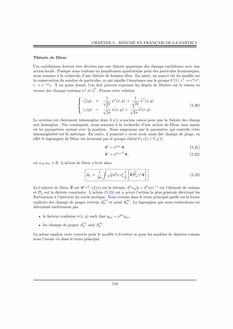
CHAPTER 5. RÉSUMÉ EN FRANÇAIS DE LA PARTIE I
Théorie de Dirac
Ces corrélations doivent être décrites par une théorie quantique des champs euclidienne avec uneaction locale. Puisque nous traitons un hamiltonien quadratique pour des particules fermioniques,nous sommes à la recherche d’une théorie de fermion libre. En outre, un aspect clé du modèle estla conservation du nombre de particules, ce qui signifie l’invariance par le groupe U(1), c† → eiϕc†,c → e−iϕc. À un point donné, l’on doit pouvoir exprimer les degrés de libertés sur le réseau entermes des champs continus ψ† et ψ
†. Fixons cette relation
c†x(y) =
1√2π
ψ†(x, y) +1√2π
ψ†(x, y)
cx(y) =1√2π
ψ(x, y) +1√2π
ψ(x, y) .(5.20)
Le système est clairement inhomogène donc il n’y a aucune raison pour que la théorie des champsoit homogène. Par conséquent, nous sommes à la recherche d’une action de Dirac sans masseoù les paramètres varient avec la position. Nous supposons que le paramètre qui contrôle cetteinhomogénéité est la métrique. En outre, il pourrait y avoir avoir aussi des champs de jauge, eneffet le lagrangien de Dirac est invariant par le groupe chiral UV (1)× UA(1)
Ψ′ = eiαV Ψ (5.21)
Ψ′ = eiαAγ5
Ψ, (5.22)
où αA, αV ∈ R. L’action de Dirac s’écrit alors
S0 =1
2π
∫ √g d2x eµa
12
[Ψ
↔
DµγaΨ]
(5.23)
Ici,l’adjoint de Dirac Ψ est Ψ†γ2, eµa(x) est la tétrade, d2x√g = d2x|e|−1 est l’élément de volume
et Dµ est la dérivée covariante. L’action (5.23) est a priori l’action la plus générale décrivant lesfluctuations à l’intérieur du cercle arctique. Nous verrons dans le texte principal quelle est la formeexplicite des champs de jauges vecteur A(v)
µ et axial A(a)µ . Le lagrangien que nous recherchons est
déterminé entièrement par
• le facteur conforme σ(x, y) such that gµν = e2σηµν ,
• les champs de jauges A(v)µ and A
(a)µ .
La même analyse reste correcte pour le modèle à 6-vertex et pour les modèles de dimères commenous l’avons vu dans le texte principal.
118

PARTIICritical properties of interface growth
models
119

CHAPTER 6. INTRODUCTION TO INTERFACE: MARKOV PROCESSES ANDSCALING BEHAVIOR
CHAPTER6Introduction to interface: Markov processes and
scaling behavior
Contents
6.1 Markov formalism . . . . . . . . . . . . . . . . . . . . . . . . . . . . . . 121
6.1.1 Interface as a stochastic process . . . . . . . . . . . . . . . . . . . . . . . 121
6.1.2 From a master equation to a Fokker-Planck equation . . . . . . . . . . . 122
6.1.3 Langevin equation . . . . . . . . . . . . . . . . . . . . . . . . . . . . . . 122
6.2 Interface growth process with diffusion . . . . . . . . . . . . . . . . . 123
6.2.1 Deposition-relaxation processes . . . . . . . . . . . . . . . . . . . . . . . 123
6.2.2 Restricted solid on solid processes . . . . . . . . . . . . . . . . . . . . . 125
6.2.3 Other processes and universality classes . . . . . . . . . . . . . . . . . . 127
6.3 Critical behavior . . . . . . . . . . . . . . . . . . . . . . . . . . . . . . . 128
6.3.1 Langevin equation and scaling properties . . . . . . . . . . . . . . . . . 128
6.3.2 Field theory formalism and ageing phenomena . . . . . . . . . . . . . . 130
6.3.3 KPZ equation . . . . . . . . . . . . . . . . . . . . . . . . . . . . . . . . . 131
120

CHAPTER 6. INTRODUCTION TO INTERFACE: MARKOV PROCESSES ANDSCALING BEHAVIOR
In this chapter, we are interesting in deriving continuous models of growing interfacestarting from a microscopic process on a lattice. In the following on considers only the 1d situationeven tough the generalization is strait forward. The simplest microscopic process on can consideris just simple random deposition of particles on a one-dimensional substrate (see Fig. 6.1), andthe question is how the interface created by this deposition will look like at large scale and howcan we describe this system as a statistical system of a continuous field. The strategy that weshall follow consist to consider the process as a Markov process and to derive the master equationfor probabilities in this process and goes to a continuum description through Fokker-Planck andLangevin equations. This formalism will lead us to the derivation of continuum equations for the
h(x, t)
x
Figure 6.1: Random deposition process. The interface of the deposition is indicated by the blueparticles.
height of the interface, and we will present two different cases known as the Edwards-Wilkinsonequation and Kardar-Parisi-Zhang equation starting from some microscopic deposition on a 1dsubstrate. We will conclude this chapter mentioning some critical properties of these equations,which lead us to two different universality classes for interface growth processes.
6.1 Markov formalism
6.1.1 Interface as a stochastic process
As we said earlier, one considers a deposition of particles on a substrate with some rates which canbe more or less complicated. We start by writing down a very general master equation describingthe stochastic evolution of a random interface in any dimension. Let us note {h} = {h0, h1...} theheight of every discrete site hi ∈ N on the lattice with periodic boundary conditions h1 = hN+1.In the following we shall work on the 1d lattice of length N . For any discrete time step, oneallows for the deposition of one particle of the substrate according to specific rules. One defines{s} = {s0, s1...}, the set of jumps after this time interval, more precisely if we depose a particle atsite k, then {s} = {0, 0..., sk = a, ..., 0, 0}, where a is a constant.
121

CHAPTER 6. INTRODUCTION TO INTERFACE: MARKOV PROCESSES ANDSCALING BEHAVIOR
6.1.2 From a master equation to a Fokker-Planck equation
The derivation here follows [207, 168, 41] and we report the reader to these references for moredetailed calculation and references. We define P({h}, t) the joint probability that, at time t, thesurface is in the state {h} et we define transition rates between two states as W({h} → {h′}) insuch way that we can write formally a master equation as
P({h}, t+δt)−P({h}, t) =∑
{s}
W({h−s} → {h}) P({h−s}, t)−W({h} → {h+s}) P({h}, t). (6.1)
We make the assumption here that the process is markovian, i.e. the state of the surface attime t + δt depends only of the state at time t, there is no memory effects and the transitionrates follow a Chapman Kolmogorov equation. Our goal is to find a proper continuum limit ofthis kind of process, when the size of the jump goes to zero. The standard way to proceed isthrough a Kramers-Moyal expansion of the master equation in order to find a partial differentialequation for the probability distribution P({h}, t). The full calculation is not very insightful (see[207] for details), and gives at second-order expansion the so-called Fokker-Planck equation for theprobability distribution
∂P
∂t′= −
∑
i
∂hi(M (1)
i P) +12
∑
i,j
∂hihj(M (2)
ij P), (6.2)
where
M(1)i =
∫ N∏
k=1
dsik si W({h} → {h+ s}), (6.3)
M(2)i,j =
∫ N∏
k=1
dsik sisj W({h} → {h+ s}). (6.4)
6.1.3 Langevin equation
For any Fokker-Planck equation, we can write a partial differential equation for the stochasticvariables directly, here for the height hi of the interface on every site
∂hi∂t′
= M(1)i + ηi, (6.5)
with
〈ηi〉 = 0, (6.6)
〈ηi(t′)ηj(t′ + τ)〉 = M(2)ij δτ . (6.7)
The Fokker-Planck equation and the Langevin equation are formally equivalent, but some featuresare more tractable with one or the other equation. In the following we will be interested computingquantities like the average or the fluctuation of the interface which can be simply done using theLangevin equation.
122

CHAPTER 6. INTRODUCTION TO INTERFACE: MARKOV PROCESSES ANDSCALING BEHAVIOR
Random deposition processes
In a purely randomly process (see Fig. 6.1), the deposition is completely independent from site tosite, then when a particle is placed at site i, only this site is affected. The transition rates can bewritten as
W({h} → {h′}) = ΓL∑
i=0
δsi,1
∏
j 6=i
δsj ,0, (6.8)
then we can compute the two first moment of this process to get the corresponding Langevinequation
M(1)i =
∫ds1 ds2...dsL si Γ
L∑
i=0
δsi,1
∏
j 6=i
δsj ,0 = Γa, (6.9)
M(2)i,j =
∫ds1 ds2...dsL sisj Γ
L∑
i=0
δsi,1
∏
j 6=i
δsj ,0 = Γa2δij . (6.10)
Finally the Langevin equation is just the equation of N uncoupled brownian motions
dhidt′
= Γa+ ξi (6.11)
with ξi are uncorrelated centered white noises
〈ξi〉 = 0, (6.12)
〈ξi(t′)ξj(t′ + τ)〉 = Γa2δijδτ . (6.13)
The solution is simply
h(x, t) = Γt′ +∫ t′
0
du ξ(x, u). (6.14)
Therefor, the interface grows linearly and the fluctuations are given by brownian motion.
6.2 Interface growth process with diffusion
6.2.1 Deposition-relaxation processes
The first step in the description of a more realistic model of interface than the brownian interfaceis to add diffusion in the process. The simplest diffusion process is to allowed particles to jumpof one site to the left or to the right with a fixed probability once they are on the interface (seeFig. 6.2). This process is know as the Family process [67]. The transition rates can be written as
W({h} → {h′}) = ΓN∑
i=0
{ω0i δsi,1
∏
j 6=i
δsj ,0 + ωdi δsi+1,1
∏
j 6=i+1
δsj ,0 + ωgi δsi−1,1
∏
j 6=i−1
δsj ,0}. (6.15)
More precisely, when a particle drops at site i, it stays at this location if the heights of the right
123
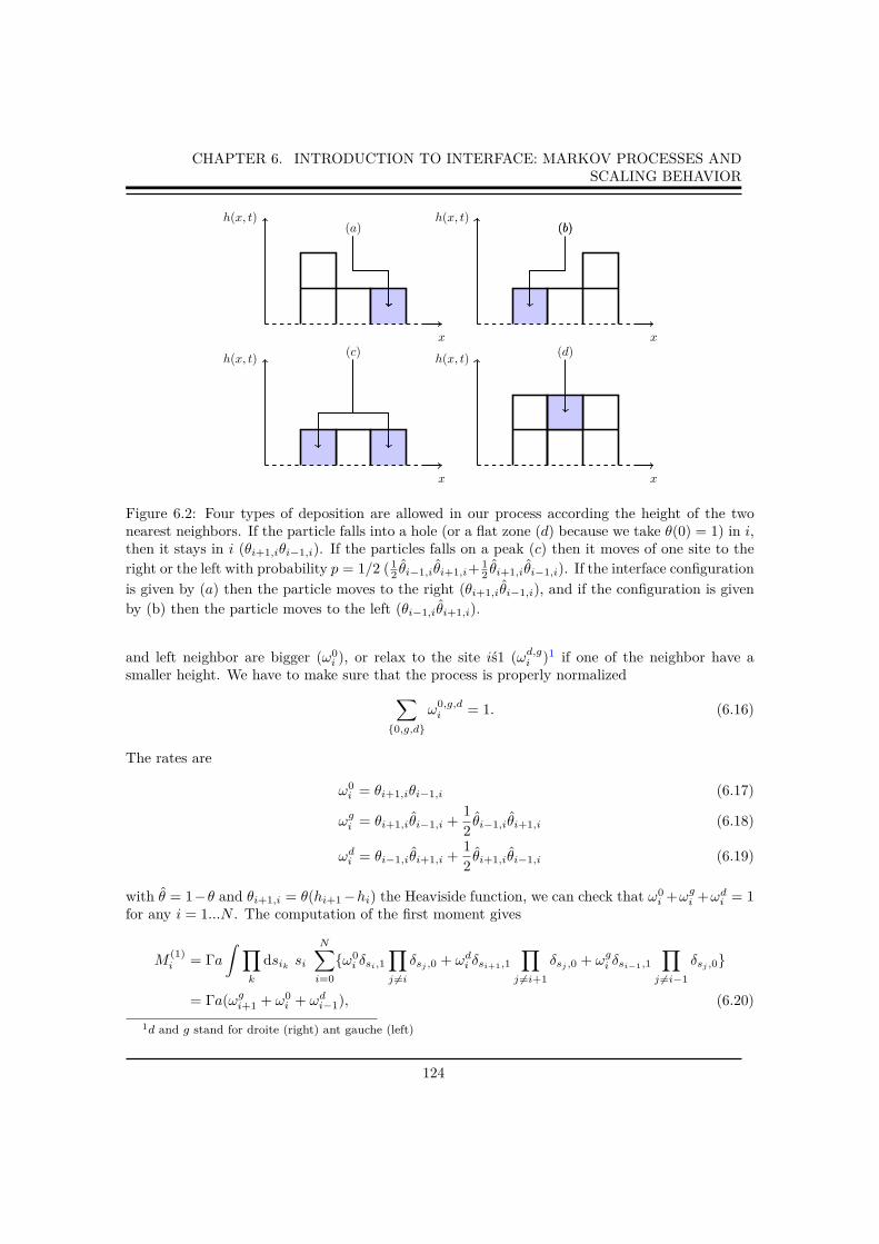
CHAPTER 6. INTRODUCTION TO INTERFACE: MARKOV PROCESSES ANDSCALING BEHAVIOR
(a)h(x, t)
x
(b)h(x, t)
x(d)
(b)
h(x, t)
x
(c)h(x, t)
x
Figure 6.2: Four types of deposition are allowed in our process according the height of the twonearest neighbors. If the particle falls into a hole (or a flat zone (d) because we take θ(0) = 1) in i,then it stays in i (θi+1,iθi−1,i). If the particles falls on a peak (c) then it moves of one site to theright or the left with probability p = 1/2 ( 1
2 θi−1,iθi+1,i+ 12 θi+1,iθi−1,i). If the interface configuration
is given by (a) then the particle moves to the right (θi+1,iθi−1,i), and if the configuration is givenby (b) then the particle moves to the left (θi−1,iθi+1,i).
and left neighbor are bigger (ω0i ), or relax to the site iś1 (ωd,gi )1 if one of the neighbor have a
smaller height. We have to make sure that the process is properly normalized∑
{0,g,d}
ω0,g,di = 1. (6.16)
The rates are
ω0i = θi+1,iθi−1,i (6.17)
ωgi = θi+1,iθi−1,i +12
θi−1,iθi+1,i (6.18)
ωdi = θi−1,iθi+1,i +12
θi+1,iθi−1,i (6.19)
with θ = 1−θ and θi+1,i = θ(hi+1−hi) the Heaviside function, we can check that ω0i +ωgi +ωdi = 1
for any i = 1...N . The computation of the first moment gives
M(1)i = Γa
∫ ∏
k
dsik si
N∑
i=0
{ω0i δsi,1
∏
j 6=i
δsj ,0 + ωdi δsi+1,1
∏
j 6=i+1
δsj ,0 + ωgi δsi−1,1
∏
j 6=i−1
δsj ,0}
= Γa(ωgi+1 + ω0i + ωdi−1), (6.20)
1d and g stand for droite (right) ant gauche (left)
124

CHAPTER 6. INTRODUCTION TO INTERFACE: MARKOV PROCESSES ANDSCALING BEHAVIOR
then the second moment
M(2)ij = Γa2
∫ ∏
k
dsik sisjN∑
i=0
{ω0i δsi,1
∏
j 6=i
δsj ,0 + ωdi δsi+1,1
∏
j 6=i+1
δsj ,0 + ωgi δsi−1,1
∏
j 6=i−1
δsj ,0}
= Γa2δij(ωgi+1 + ω0
i + ωdi−1). (6.21)
Now that we have express the quantities M(1)i and M
(2)ij as function of the microscopic rates of
deposition of particles on the lattice, we can formally expand the difference of height between twoneighboring site as
hi±1 − hi =∑
k
(±a)k
k!∂kh(x)
∂xk
∣∣∣(x=ia)
, (6.22)
Now we can use a formal regularization of the Heaviside distribution
θ(x) = lima→0
θa(x), (6.23)
where θa(x) is a differentiable function. Using the expansion of the function
θa(x) = 1 +∑
ckxk. (6.24)
Now we use this expansion on the discrete Langevin equation to get
Γa (ωgi+1 + ω0i + ωdi−1)→ cst + ν∇2
ihi +O(a3) (6.25)
Then on can write∂th = v + ν∂2
xh + ξ(x, t), (6.26)
where ν = Γa2. This method does not seem very mathematically well defined because of thisexpansion of the Heaviside function. Nevertheless it gives a fairly good result at the end. Theonly annoying problem is that the macroscopic parameters are not uniquely define in terms of themicroscopic parameters because of the choice of the function θa(x), in this case the constant v willdepend on that. We will come back to that later in the case of KPZ equation. This equation iscalled the Edwards Wilkinson [62], it is nothing but a diffusion equation for the height variablewith a gaussian noise, and can be easily solved by means of Fourier transform in any dimension.
6.2.2 Restricted solid on solid processes
Now we choose other types of depositions which can be think as constrained random depositions,known as restricted solid-on solid models. The simplest one is the Kim-Kosterlitz process [131] thatwe shall detailed in the following. The RSOS processes, are not standard processes of deposition ofparticles on a substrate because any diffusion processes are forbidden. A particle is dropped on thesurface only under a restricting condition between difference of height between nearest neighbors.In the following we shall study a particular case known as the Kim-Kosterlitz restriction, where thedifference is always less that one unit of height i.e. |hi − hi±1|ša. The continuum derivation seen
125

CHAPTER 6. INTRODUCTION TO INTERFACE: MARKOV PROCESSES ANDSCALING BEHAVIOR
on the previous chapter can be applied to this process as well. In comparison to the deposition-relaxation seen before, the rates to go left or right are zero (ωd = ωg = 0) and only the rate ω0
arises in the master equation
W({h} → {h′}) = ΓL∑
i=0
ωiδsi,1
∏
j 6=i
δsj ,0, (6.27)
with ωi = θi+1,iθi−1,i. We can easily understand that if the interface is initially flat hi = 0, then thechoice of this rate will create an interface over time that will respect the Kim-Kosterlitz restriction|hi − hi±1|ša. Now we can proceed in the exact same way as for the previous model and computethe two first moments of the Kramers-Moyal expansion
M(1)i =
∫ds1 ds2... dsL si Γ
L∑
i=0
ωiδsi,1
∏
j 6=i
δsj ,0 = ΓaÊωi, (6.28)
M(2)i,j =
∫ds1 ds2... dsL sisj Γ
L∑
i=0
ωiδsi,1
∏
j 6=i
δsj ,0 = Γa2ωiδij . (6.29)
And then the discrete Langevin equation for the height at site i follows
dhidt
= M(1)i + ηi (6.30)
with with ξi are uncorrelated centered white noises
〈ηi〉 = 0, (6.31)
〈ηi(t′)ηj(t′ + τ)〉 = Γa2δijδτ . (6.32)
The discrete Langevin equation can be written ∀i as
dhidt
= Γa θi+1,iθi−1,i + ηi(t) (6.33)
where θi+1,i := θ(hi+1− hi), θ(0) = 1 and ηi is the discrete white noise. In the RSOS process, onehave hi±1 − hi ∼ O(a). Now we can use a formal regularization of the Heaviside distribution
θ(x) = lima→0
θa(x) (6.34)
where θa(x) is a differentiable function. Using the expansion of the function
θa(x) = 1 +∑
ckxk (6.35)
Now we use this expansion on the discrete Langevin equation
∂h(x, t)∂t
= Γa[1 + a2c1
∂2h
∂x2+ (2c2a2 − c2
1a2)(∂h
∂x
)2
+O(a3)]
+ η (6.36)
We define Γa2 → ν in the thermodynamic limit, as the diffusive parameter which is always constant.Here, we notice that the factor in front of the non-linear (we call it λ) term is not wheel defined
126

CHAPTER 6. INTRODUCTION TO INTERFACE: MARKOV PROCESSES ANDSCALING BEHAVIOR
because Γa(2c2a2 − c2
1a2) goes to infinity when a → 0 (λ ∼ O(Γa) → ∞) because cp ∼ O(a−p).
With this method the nonlinear coupling of the theory is diverging when the lattice unit goes tozero, so the theory is not coherent and the macroscopic quantities cannot be interpreted usingmicroscopic parameters. One can mention that this divergence can be avoiding using the samemethod with small modifications in the definition of the space derivative, leading to the exact sameform for the continuum equation with different explicit expression for the macroscopic parameters.Finally on can argue that this ”master equation to Langevin equation” derivation gives the rightanswer for the form of the macroscopic equation but not the explicit relation between parameters.
t = 0
t = 1 t = 1t = 1 t = 2 t = 2 t = 2
t = 3
t = 3 t = 3t = 4
t = 4 t = 4t = 5 t = 5 t = 5
h(x, t)
x
Figure 6.3: Kim-Kosterlitz process on a 1d substrate. The initial state at t = 0 is the whiteflat interface, then a fixed (3 in the figure) number of particles can reached the substrate if thecondition |hi±1 − hi|ša is fulfilled, at each time (t = 1 red particles, t = 2 blue particles...).
6.2.3 Other processes and universality classes
There exists a lot of microscopic processes that leads to the same scaling limit of the EW andKPZ equation. But not all the processes fall into this two classes. Another class is governed bythe Mullins-Herring equation
∂th = −κ∂4xh+ ξ(x, t), (6.37)
where ξ is a gaussian white noise. This equation is particularly useful in the context of molecularbeam epitaxy (see [14] for an overview). We do not want to enter into these details but let us juststress that one microscopic process that gives this equation in the scaling limit is the so-called Wolf-Villain process described on Fig. 6.4. To include some surface relaxation, we allow the depositedparticle to diffuse along the surface up to a finite distance, stopping when it finds the position withthe lowest height. As we shall see later, those three equations (EW, MH and KPZ) are the mainclasses of non-disorder interface growth processes. They define three universality classes definedby a set of critical exponents that we shall briefly detailed in the following.
127

CHAPTER 6. INTRODUCTION TO INTERFACE: MARKOV PROCESSES ANDSCALING BEHAVIOR
Figure 6.4: Wolf-Villain process on a one-dimensional substrate
6.3 Critical behavior
Interface growth processes are dynamical, out of equilibrium phenomena that can be describedby Langevin equations for a ”order parameter” (in that case the height h(x, t)). Contrary toequilibrium (or non-equilibrium) critical phenomena, there is no strict phase transition in thesemodels but a critical behavior of fluctuations. As we said before, the concept of renormalizationapply in these problems leading to different universality classes for interface growth processes. Thelanguage of usual critical phenomena is then used in a broader sense, and the notion of universalityclass of interface can be defined.
6.3.1 Langevin equation and scaling properties
In this chapter, we shall briefly recall some of the main critical features of interface growth equa-tions. The simplest non-trivial equation describing the fluctuation of an interface due to deposition-relaxation process is, as we have seen before, the Edwards-Wilkinson equation
∂th(x, t) = ν∂2xh(x, t) + η(x, t), (6.38)
where η is a gaussian white noise,
〈η(x, t)〉 = 0 (6.39)
〈η(x, t)η(x′, t′)〉 = 2Dδ(x− x′)δ(t− t′). (6.40)
This equation is the continuum limit of a many microscopic processes and its resolution is verysimple du to the linearity of the equation. The resolution leads to a set of critical exponents whichcharacterize the EW universality class. The scaling hypothesis is a powerful tool to find criticalexponents very easily, in the case of fractal interface, we rescale the height, and the space-time asfollows
x→ x′ = bx (6.41)
t→ t′ = bzt (6.42)
h→ h′ = bαh, (6.43)
where α, z are two exponents which characterize the universality class of the growth process. Thestatistical properties of the interface must be unchanged under this transformation. The EW
128

CHAPTER 6. INTRODUCTION TO INTERFACE: MARKOV PROCESSES ANDSCALING BEHAVIOR
equation reads∂th(x, t)− ν∇2h(x, t) = η(x, t). (6.44)
After the transformation, it becomes
bα−z∂th(x, t)− bα−2ν∇2h(x, t) = b−z/2−d/2η(x, t), (6.45)
∂th(x, t)− bz−2ν∇2h(x, t) = bz/2−d/2−αη(x, t). (6.46)
The invariance of the equation under this transformation enforces
bz−2ν∇2h(x, t) + bz/2−d/2−αη(x, t) = ν∇2h(x, t) + η(x, t), (6.47)
gives us the values of z and α
α =2− d
2(6.48)
β =2− d
4(6.49)
z = 2, (6.50)
which leads in 1d, to β = 1/4, z = 2 and α = 1/2. Let us notice that the upper critical dimensionof the EW equation is dc = 2, where α = β = 0. The value of dc for KPZ equation is not clear,and very controversial, opinions vary between dc = 2.4 and dc = ∞. In the random depositionprocess, each particle falls on a single site on the top of the surface and it sticks irreversibly. A aresult of the relaxation process, the final interface will be smooth compared to a model withoutrelaxation. This process generates correlations among the neighboring heights, which leads to anentire correlated interface and resulting in the saturation of the interface. Numerical simulationsof a system of size L with periodic boundary conditions give the following scaling behavior
wL(t) =∫
dx√〈h(x, t)2〉 − 〈h(x, t)〉2 = Lαf(tL−z), (6.51)
where f is a scaling function which interpolates between short times t << Lz
limu→0
f(u) = uβ , (6.52)
and long times t >> Lz with the asymptotic behavior
limu→∞
f(u) = cst, (6.53)
which means that w(t) ∼ tβ for a time smaller than the correlation time Lz and reaches thesaturation value for time bigger than the correlation time. This asymptotic form of the scalingfunction called the Family-Viczek scaling impose relation between exponents
z =α
β. (6.54)
This relation is valid for any equation satisfying the Family-Viczek scaling.
129

CHAPTER 6. INTRODUCTION TO INTERFACE: MARKOV PROCESSES ANDSCALING BEHAVIOR
0 200 400 600 800 1000
�2
0
2
4
t1
t2
t3
Figure 6.5: h−〈h〉 in the Kim-Kosterlitz process for 3 different times t1 < t2 < t3 of size L = 1000with periodic boundary conditions.
6.3.2 Field theory formalism and ageing phenomena
The field theory describing a growth process like the Edwards-Wilkinson or the Kardar-Parisi-Zhang equation is very well known. The Janssen-De dominicis action is given by
S[h, h] =
∫ddx
∫dt h (∂th+
δH[h]
δh)− νh2 (6.55)
where −H[h] is the Ginsburg-Landau hamiltonian which may content all the possible derivativesand nonlinear terms and we note x the d-dimensional spatial vector. We define the 2-point spacio-temporel correlations function by
C(x, y, t, s) = 〈h(x, t)h(y, s)〉, (6.56)
and the 2-point spatio-temporel response function by
R(x, y, t, s) = limh→0
δh(x, t)
δj(y, s)= 〈h(x, t)h(y, s)〉. (6.57)
Let us point out the fact that the field h has no real physical meaning, except the property that itscorrelation with h(x, t) gives the response function. The corresponding Langevin equation whichcan be derive from the action by integration over the response field h is
∂th+δH[h]
δh= η, (6.58)
130
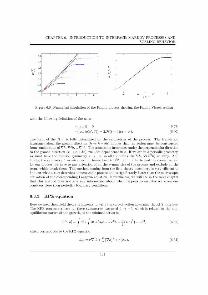
CHAPTER 6. INTRODUCTION TO INTERFACE: MARKOV PROCESSES ANDSCALING BEHAVIOR
t/Lz
w(t)/Lα
Figure 6.6: Numerical simulation of the Family process showing the Family Viczek scaling
with the following definition of the noise
〈η(x, t)〉 = 0 (6.59)
〈η(x, t)η(x′, t′)〉 = 2Dδ(t− t′)(x− x′). (6.60)
The form of the H[h] is fully determined by the symmetries of the process. The translationinvariance along the growth direction (h → h + δh) implies that the action must be constructedfrom combination of∇h, ∇2h, ...∇nh. The translation invariance under the perpendicular directionto the growth direction (x→ x+ δx) excludes dependence in x. If we are in a periodic geometry,we must have the rotation symmetry x → −x, so all the terms like ∇h, ∇(∇2h) go away. Andfinally, the symmetry h → −h rules out terms like (∇h)2p. So in order to find the correct actionfor our process, we have to pay attention of all the symmetries of the process and exclude all theterms which break them. This method coming from the field theory machinery is very efficient tofind out what action describes a microscopic process and is significantly faster than the microscopicderivation of the corresponding Langevin equation. Nevertheless, we will see in the next chapterthat this method does not give any information about what happens to an interface when oneconsiders close (non-periodic) boundary conditions.
6.3.3 KPZ equation
Here we used these field theory arguments to write the correct action governing the KPZ interface.The KPZ process respects all these symmetries excepted h → −h, which is related to the non-equilibrium nature of the growth, so the minimal action is
S[h, h] =
∫ddx
∫dt h
(∂tφ− ν∇2h− µ
2
(∇h)2)− νh2, (6.61)
which corresponds to the KPZ equation
∂th = ν∇2h+µ
2
(∇h)2
+ η(x, t). (6.62)
131
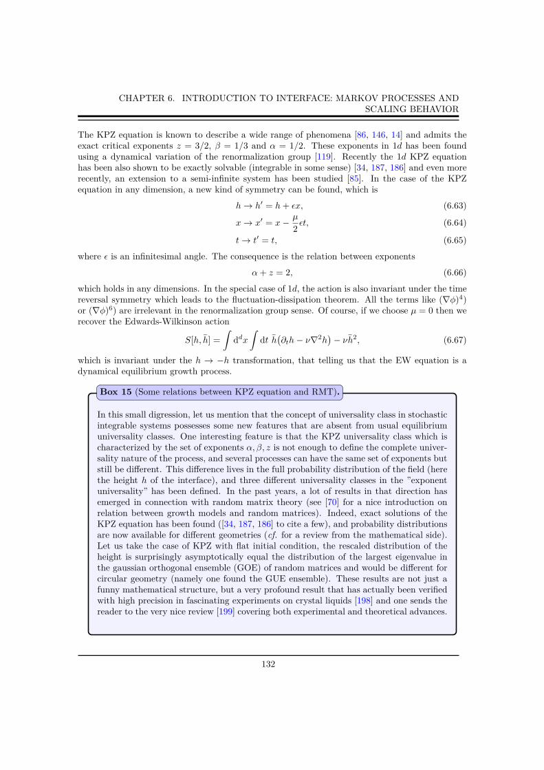
CHAPTER 6. INTRODUCTION TO INTERFACE: MARKOV PROCESSES ANDSCALING BEHAVIOR
The KPZ equation is known to describe a wide range of phenomena [86, 146, 14] and admits theexact critical exponents z = 3/2, β = 1/3 and α = 1/2. These exponents in 1d has been foundusing a dynamical variation of the renormalization group [119]. Recently the 1d KPZ equationhas been also shown to be exactly solvable (integrable in some sense) [34, 187, 186] and even morerecently, an extension to a semi-infinite system has been studied [85]. In the case of the KPZequation in any dimension, a new kind of symmetry can be found, which is
h→ h′ = h+ ǫx, (6.63)
x→ x′ = x− µ
2ǫt, (6.64)
t→ t′ = t, (6.65)
where ǫ is an infinitesimal angle. The consequence is the relation between exponents
α+ z = 2, (6.66)
which holds in any dimensions. In the special case of 1d, the action is also invariant under the timereversal symmetry which leads to the fluctuation-dissipation theorem. All the terms like (∇φ)4)or (∇φ)6) are irrelevant in the renormalization group sense. Of course, if we choose µ = 0 then werecover the Edwards-Wilkinson action
S[h, h] =
∫ddx
∫dt h
(∂th− ν∇2h
)− νh2, (6.67)
which is invariant under the h → −h transformation, that telling us that the EW equation is adynamical equilibrium growth process.
In this small digression, let us mention that the concept of universality class in stochasticintegrable systems possesses some new features that are absent from usual equilibriumuniversality classes. One interesting feature is that the KPZ universality class which ischaracterized by the set of exponents α, β, z is not enough to define the complete univer-sality nature of the process, and several processes can have the same set of exponents butstill be different. This difference lives in the full probability distribution of the field (herethe height h of the interface), and three different universality classes in the ”exponentuniversality” has been defined. In the past years, a lot of results in that direction hasemerged in connection with random matrix theory (see [70] for a nice introduction onrelation between growth models and random matrices). Indeed, exact solutions of theKPZ equation has been found ([34, 187, 186] to cite a few), and probability distributionsare now available for different geometries (cf. for a review from the mathematical side).Let us take the case of KPZ with flat initial condition, the rescaled distribution of theheight is surprisingly asymptotically equal the distribution of the largest eigenvalue inthe gaussian orthogonal ensemble (GOE) of random matrices and would be different forcircular geometry (namely one found the GUE ensemble). These results are not just afunny mathematical structure, but a very profound result that has actually been verifiedwith high precision in fascinating experiments on crystal liquids [198] and one sends thereader to the very nice review [199] covering both experimental and theoretical advances.
Box 15 (Some relations between KPZ equation and RMT).
132

CHAPTER 7. BOUNDARY INTERFACE GROWTH PROCESSES
CHAPTER7Boundary interface growth processes
Contents
7.1 Interface growth near a boundary . . . . . . . . . . . . . . . . . . . . 134
7.1.1 Introduction to the problem . . . . . . . . . . . . . . . . . . . . . . . . . 134
7.1.2 Deposition-relaxation process with a boundary . . . . . . . . . . . . . . 135
7.1.3 Continuum Langevin equation . . . . . . . . . . . . . . . . . . . . . . . 137
7.2 Exact solution of the model and numerical comparison . . . . . . . 138
7.2.1 Laplace transform and exact solution . . . . . . . . . . . . . . . . . . . . 139
7.2.2 Mean profile of the interface . . . . . . . . . . . . . . . . . . . . . . . . . 142
7.2.3 Fluctuation of the height of the interface . . . . . . . . . . . . . . . . . 145
7.3 Boundary KPZ equation . . . . . . . . . . . . . . . . . . . . . . . . . . 151
7.3.1 Introduction and definition of the problem . . . . . . . . . . . . . . . . . 152
7.3.2 KPZ equation with a boundary . . . . . . . . . . . . . . . . . . . . . . . 153
7.3.3 Scaling hypothesis and numerical results . . . . . . . . . . . . . . . . . . 153
7.4 Conclusions . . . . . . . . . . . . . . . . . . . . . . . . . . . . . . . . . . 156
133
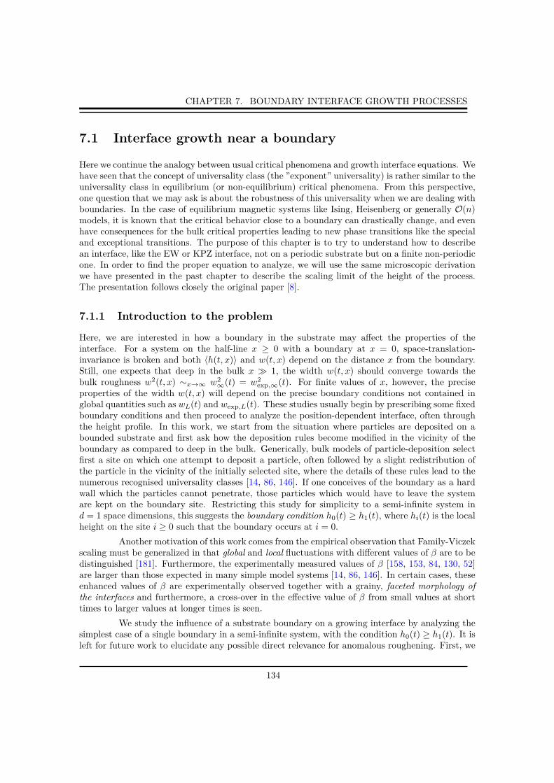
CHAPTER 7. BOUNDARY INTERFACE GROWTH PROCESSES
7.1 Interface growth near a boundary
Here we continue the analogy between usual critical phenomena and growth interface equations. Wehave seen that the concept of universality class (the ”exponent” universality) is rather similar to theuniversality class in equilibrium (or non-equilibrium) critical phenomena. From this perspective,one question that we may ask is about the robustness of this universality when we are dealing withboundaries. In the case of equilibrium magnetic systems like Ising, Heisenberg or generally O(n)models, it is known that the critical behavior close to a boundary can drastically change, and evenhave consequences for the bulk critical properties leading to new phase transitions like the specialand exceptional transitions. The purpose of this chapter is to try to understand how to describean interface, like the EW or KPZ interface, not on a periodic substrate but on a finite non-periodicone. In order to find the proper equation to analyze, we will use the same microscopic derivationwe have presented in the past chapter to describe the scaling limit of the height of the process.The presentation follows closely the original paper [8].
7.1.1 Introduction to the problem
Here, we are interested in how a boundary in the substrate may affect the properties of theinterface. For a system on the half-line x ≥ 0 with a boundary at x = 0, space-translation-invariance is broken and both 〈h(t, x)〉 and w(t, x) depend on the distance x from the boundary.Still, one expects that deep in the bulk x ≫ 1, the width w(t, x) should converge towards thebulk roughness w2(t, x) ∼x→∞ w2
∞(t) = w2exp,∞(t). For finite values of x, however, the precise
properties of the width w(t, x) will depend on the precise boundary conditions not contained inglobal quantities such as wL(t) and wexp,L(t). These studies usually begin by prescribing some fixedboundary conditions and then proceed to analyze the position-dependent interface, often throughthe height profile. In this work, we start from the situation where particles are deposited on abounded substrate and first ask how the deposition rules become modified in the vicinity of theboundary as compared to deep in the bulk. Generically, bulk models of particle-deposition selectfirst a site on which one attempt to deposit a particle, often followed by a slight redistribution ofthe particle in the vicinity of the initially selected site, where the details of these rules lead to thenumerous recognised universality classes [14, 86, 146]. If one conceives of the boundary as a hardwall which the particles cannot penetrate, those particles which would have to leave the systemare kept on the boundary site. Restricting this study for simplicity to a semi-infinite system ind = 1 space dimensions, this suggests the boundary condition h0(t) ≥ h1(t), where hi(t) is the localheight on the site i ≥ 0 such that the boundary occurs at i = 0.
Another motivation of this work comes from the empirical observation that Family-Viczekscaling must be generalized in that global and local fluctuations with different values of β are to bedistinguished [181]. Furthermore, the experimentally measured values of β [158, 153, 84, 130, 52]are larger than those expected in many simple model systems [14, 86, 146]. In certain cases, theseenhanced values of β are experimentally observed together with a grainy, faceted morphology ofthe interfaces and furthermore, a cross-over in the effective value of β from small values at shorttimes to larger values at longer times is seen.
We study the influence of a substrate boundary on a growing interface by analyzing thesimplest case of a single boundary in a semi-infinite system, with the condition h0(t) ≥ h1(t). It isleft for future work to elucidate any possible direct relevance for anomalous roughening. First, we
134

CHAPTER 7. BOUNDARY INTERFACE GROWTH PROCESSES
shall study the semi-infinite 1d Edwards-Wilkinson (ew) model [62], whose bulk behavior is well-understood from an exact solution. We shall write down a physically correct Langevin equationin semi-infinite space which includes this new kind of boundary contribution. Its explicit exactsolution, of both the height profile as well as the site-dependent interface width, will be seento be in agreement with a large-scale Monte Carlo (mc) simulations. It turns out that thereexists a surprisingly large intermediate range of times where the model crosses over to a new fixedpoint, with an effective and non-trivial surface growth exponent β1,eff > β, which is qualitativelyanalogous to the experiments cited above. However, at truly large times, typically above thediffusion time, the system converts back to the fv scaling, as expected from the bulk rg [150].Second, in order to show that these observations do not come from the fact that the Langevinequation of the ew model is linear, we present numerical data for a model in the universality classof the semi-infinite 1d Kardar-Parisi-Zhang (kpz) equation [119]. We find the same qualitativeresults as for the ew class, with modified exponents. We point out that the time scales needed tosee these cross-overs are considerably larger than those studied in existing experiments.
7.1.2 Deposition-relaxation process with a boundary
In this section we want to generalize the deposition-relaxation process that we have presented inthe periodic boundary conditions case in the previous chapter, for a non-translational invariantsituation. We have in mind to build a deposition process on the semi-infinite line (i = 1, 2...)with some wall at the origin. There are many possibilities to this process, but we want to do the
i = 1 i = 2 i = 3 i = 4 i = 5 i = 6 ...
hi(t)
BOUNDARY
i
Figure 7.1: Etat initial plat d’un processus de croissance semi-infini
simplest thing possible, i.e. the process in the bulk has to be the same as for the periodic case,and the presence of the wall is purely geometric and do not add some other physical phenomena.To be clear, we need to express the transition rates when particles fall down close to the wall. Therules is that the wall is impenetrable, which means that a particle which deposit in i = 1 can stickto this site or move to i = 2 with some rates but not diffuse to i = 0. In that particular model, theonly rates that will change are those in i = 1 and i = 2 and all the others will be the same, we willuse the notation ω for rates which are different from the periodic case. With those notations therates ω0
1 and ωd1 in i = 1 and i = 2 will be For more generality we can assume a small transition ǫ
135

CHAPTER 7. BOUNDARY INTERFACE GROWTH PROCESSES
h(x, t)BOUNDARY (a)
x
h(x, t)
BOUNDARY (b)
x
Figure 7.2: Modification of the transition rates close to the wall. Case (a) corresponds to transitionrate ω
(0)1 and case (b) to ω
(d)1 .
from i = 1 to i = 0, leading to a small flux of particles through the wall,
ω01 = θ21(1− ǫ) ∼ O(1) (7.1)
ωd1 = (1− ǫ)θ21 +ǫ
2θ21 ∼ O(1), (7.2)
ωg1 = ǫθ21 +ǫ
2θ21 ∼ O(ǫ), (7.3)
ωd0 = ǫθ10 +ǫ
2θ10 ∼ O(ǫ). (7.4)
In the limit ǫ→ 0, one recover ω01 = θ21, ωd1 = θ21 for a hard-wall and ωg1 = ωd0 = 0. All the others
transition rates remain the same
ω0i = θi+1,iθi−1,i, (7.5)
ωgi = θi+1,iθi−1,i +12
θi−1,iθi+1,i, (7.6)
ωdi = θi−1,iθi+1,i +12
θi+1,iθi−1,i, (7.7)
with the proper normalization∑
ωi = 1 ∀i > 1 and∑
ω1 = 1. Now that all the rates are explicitlywritten, on can write down the Langevin equation as in the previous chapter for every site fromi = 1, 2...
dh1
dt= Γa
[ω0
1 + ωg2 + ωd0
]+ η1(t), (7.8)
dh2
dt= Γa
[ω0
2 + ωg3 + ωd1
]+ η2(t), (7.9)
dhi>2
dt= Γa
[ω0i + ωgi+1 + ωdi−1
]+ ηi(t), (7.10)
which can be put in a single equation valid for every site i
dhidt
= Γa[M
(1)i +
(∆ω
(0)1 + ∆ω
(d)0
)δi,1 + ∆ω
(d)1 δi,2
]+ ηi(t), (7.11)
136

CHAPTER 7. BOUNDARY INTERFACE GROWTH PROCESSES
where ∆ω := ω − ω, correspond to corrective terms du to the boundary. Explicitely
∆ω(0)1 = ω
(0)1 − ω
(0)1 = θ21(1− ǫ)− θ21θ01 = θ21(1− ǫ− θ01), (7.12)
∆ω(d)1 = ω
(d)1 − ω
(d)1 = (1− ǫ)θ21 +
ǫ
2θ21 − θ01θ21 +
12
θ21θ01, (7.13)
∆ω(d)0 = ω
(d)0 − ω
(d)0 = ǫθ10 +
ǫ
2θ10 − θ−10θ10 +
12
θ10θ−10. (7.14)
The term ∆ω(d)0 is not relevant here because it is acting on the other side of the wall and it is of
order ǫ (indeed for a hard wall ǫ→ 0, the probability to cross the wall is zero) while the two otherterms ∆ω
(0)1 and ∆ω
(d)1 are of order 1. Then one can simply write
dhidt
= Γa[M
(1)i +
(∆ω
(0)1 + ∆ω
(d)0
)δi,1 + ∆ω
(d)1 δi,2
]+ ηi(t),
= Γa[M
(1)i +
(∆ω
(0)1 + ∆ω
(d)0
)δi,1 + ∆ω
(d)1 δi,2 + ∆ω
(d)1 δi,1 −∆ω
(d)1 δi,1
]+ ηi(t),
= Γa[M
(1)i +
(∆ω
(0)1 + ∆ω
(d)0 + ∆ω
(d)1
)δi,1 + a∆ω
(d)1
δi,2 − δi,1a
]+ ηi(t). (7.15)
We put this equation is that following form in order to make transparent the fact that this equationis exactly the same as for the periodic case (the term M
(1)i is the same, and also the noise) up to
terms that act locally on the boundary. Let us notice that, the first in δi,1 act on the boundarysite i = 1 and the second term act between i = 1 and i = 2. This last term will be absent whenwe will consider the same protocol for the Kim-Kosterlitz process because there are no diffusion inthe definition of the rates.
7.1.3 Continuum Langevin equation
It is possible to analyze the scaling limit a→ 0 of the last equation in a general way. The idea isthat, in the continuum limit where δi,1/a→ δ(x), the equation will look like
∂th(x, t) = v + ν[Mh(x, t) + P0h(0, t)δ(x) + Q0h(0, t)δ′(x)
]+ η(x, t), (7.16)
where M, P0, Q0 are differential operators. The form of the 3 operators is fully determined by thesymmetry of the process. The translation invariance along the growth direction (h→ h+δh) impliesthat the action must be constructed from combinations of ∂h, ∂2h, ...∂nh. In a semi-infinite process,the translation invariance under the perpendicular direction to the growth direction (x→ x + δx)is broken, then dependence in x is allowed. Same thing for the rotation symmetry x→ −x, so allthe terms like ∂h, ∂(∂2h) are possible. And finally The symmetry h → −h rules out terms like(∂h)2p for an equilibrium interface but are allowed for non equilibrium process. For example theKPZ process respects all this symmetries excepted h→ −h, which is related to the non equilibriumnature of the growth, finally
M = M(x, x2...∂xh, ∂2xh...(∂xh)2, (∂xh)4...) (7.17)
P0 = P0(x, x2...∂xh0, ∂2xh0...(∂xh0)2, (∂xh0)4...)
Q0 = Q0(x, x2...∂xh0, ∂2xh0...(∂xh0)2, (∂xh0)4...).
137

CHAPTER 7. BOUNDARY INTERFACE GROWTH PROCESSES
In the following we will forget about the term Q0 which is of high-order and not relevant for aphenomenological discussion. One considers now the discrete Langevin equation that we obtainEq. (7.15) and the aim is to write an continuum version of this equation for the behavior of theinterface in this setup The hypothesis is to choose the interface flat behind the wall i < 1 i.e.
h(x, t)
∂xh(0−, t)
x0
Figure 7.3: Boundary condition of the interface
θ10 = θ−10 = 1 (h′−(0) = 0 in the continuum limit), one can show that, at order a3 the only
remaining term is θ21 → [1− ac1h′+(0)], where h′
+(0) is the right derivative in x = 0. Finally, thecontinuum equation for the evolution of the interface close to a wall will take the following form
∂th(x, t) = ν∂2xh(x, t) + ν(µ1 + µ2h
′(0, t))δ(x) + η(x, t). (7.18)
In that case the operators of equation Eq. (7.16) are M = ∂2x, P0 = µ1 + µ2∂x et Q0 = 0. We
do not give the expressions of µ1 and µ2 in terms of microscopic parameters for the same reasonthat we mentioned in the previous chapter, and prefer to see this equation as a phenomenologicalequation that we will compare to numerical simulations.
7.2 Exact solution of the model and numerical comparison
In this section, the exact solution of the model is presented by mean of a spatial Laplace transform.It leads to the following form for the evolution of the height h(x, t)
∂th(x, t) = ν∂2xh(x, t) + ν
(µ1 + µ2h1(t)
)δ(x) + η(x, t), (7.19)
where we have defined h1(t) = ∂xh(x = 0, t) and η is the same gaussian white noise as usual. If,however, one wishes to model thermal equilibrium interface fluctuations, one has to consider whitenoise with the Einstein relation D = 2νkBT where T is the temperature and kB the Boltzmannconstant. In the following, we take ν = kB = 1. In order to solve this PDE we impose the initialcondition h(x, t = 0) = 0, meaning that we start with a flat interface at t = 0 and let the systemevolve according to (Eq. (8.1)). The evolution equation is linear then we can solve it by an integraltransformation.This holds in a co-moving frame with the average interface deep in the bulk (suchthat 〈h(t,∞)〉 = 0). Furthermore, ν is the diffusion constant, κ1 can be considered as an external
138

CHAPTER 7. BOUNDARY INTERFACE GROWTH PROCESSES
source at the origin and one defines h1(t) := ∂xh(t, x)|x=0. Indeed, taking the noise average of Eq.(8.1) and performing a space integration over the semi-infinite chain, we find that
ν−1∂t
∫ ∞
0
dxh(t, x) = κ1 + (κ2 − 1)h1(t). (7.20)
We take κ2 = 1 since this corresponds to the simplest condition of a constant boundary currentνκ1δ(x). The centered Gaussian noise has the variance 〈η(t, x)η(t′, x′)〉 = 2νTδ(t − t′)δ(x − x′),where T is an effective temperature. Parameters ν, κ1, and T are material-dependent constantsand initially, the interface is flat h(0, x) = 0. With respect to the well-known description of thebulk behavior, the new properties come from the boundary terms on the r.h.s. of eq. (Eq. (8.1)).In contrast to earlier studies [210], the local slope h1(t) is not a priori given, but must be foundself-consistently.
7.2.1 Laplace transform and exact solution
We define the spatial Laplace operator Lx as
Lx.h(x, t) = h∗p(t) =
∫
R+
dx e−pxh(x, t), p > 0, (7.21)
and the inverse Laplace transform
L−1p .h∗
p(t) = h(x, t) =1
2iπ
∫ i∞
−i∞
dp epxh∗p(t), x > 0, (7.22)
given the following moments of the noise η(x, t) in the p-space
〈η∗p(t)η∗
q (s)〉 =∫ ∞
0
dp∫ ∞
0
dq epx−qy 〈η(x, t)η(y, s)〉 (7.23)
= 2Tδ(t− s)∫ ∞
0
dp∫ ∞
0
dq epx−qy δ(x− y)
= 2Tδ(t− s)p+ q
,
and transforming the partial differential equation into differential equation
Lt.∂2xh(x, t) =
∫
R+
dx e−px∂2xh(x, t) (7.24)
= [e−px∂xh(x, t)]∞0 +∫
R+
dx pe−px∂xh(x, t)
= − ∂xh(x, t)x=0 + [pe−pxh(x, t)]∞0 + p2
∫
R+
dx e−pxh(x, t)
= − h′(0, t)− ph(0, t) + p2h∗(p, t),
with the assumption
limx→∞
e−pxh(x, t) = limx→∞
e−pxh′(x, t) = 0 ∀t, p ∈ R+. (7.25)
139

CHAPTER 7. BOUNDARY INTERFACE GROWTH PROCESSES
Now we start the resolution of (8.1) using Laplace transform, the initial condition h(x, t)t=0 = 0,reduces the system to
∂th∗p(t) = p2h∗
p(t)− h′(0, t)− ph(0, t) + (µ1 + µ2h′(0, t)) + η∗
p(t). (7.26)
In order to solve this non-homogenous differential equation, we use an ansatz for the solution
h∗p(t) = e−pxh∗
p(t), (7.27)
such thate−px∂th
∗p(t) = −ph(0, t) + µ1 + (µ2 − 1)h′(0, t) + η∗
p(t), (7.28)
putting this ansatz in the evolution equation gives
h∗p(t) = h∗
p(t = 0) +∫ t
0
dτ e−p2τ{−ph(0, t) + µ1 + (µ2 − 1)h′(0, t) + η∗p(t)}, (7.29)
where h∗p(t = 0) = 0 because of the initial condition h(x, t = 0) = 0, then
h∗p(t) =
∫ t
0
dτ e−p2τ{−ph(0, t) + µ1 + (µ2 − 1)h′(0, t) + η∗p(t)}. (7.30)
From now on, we will use the short hand notation h0 = h(0, t) and h′0 = h′(0, t) and define
ζ∗p (t) =
∫ t
0
dτ ep2(t−τ)η∗
p(t), (7.31)
and we can write the solution for the Laplace transform of the height as the sum of a pure noisyzero-averaged term plus a second term
h∗p(t) = ζ∗
p (t) +∫ t
0
dτ e−p2(t−τ){(µ2 − 1)h′0(τ)− ph0(τ) + µ1}. (7.32)
The Inverse Laplace transform of h∗p(t) can be solved easily as function of the initial condition
h∗p(t = 0). Then the inverse transform of h∗
p(t) is obtained by integrating over p in the complexplane along the imaginary axis, leading to Gaussian integrals, and we obtain, for the generalsolution of h(t, x)
h(x, t) = ζ(x, t) +∫ t
0
dτ1√
4π(t− τ)
((µ2 − 1)h′
0(τ) + µ1 + h0(τ)x
2(t− τ)
)e
−x2
4(t−τ) . (7.33)
We can notice that the solution is a sum of two parts, a fully noisy part, which is the same onethan in the classical EW equation, plus an another contribution coming from the boundary, whichcontains deterministic and noisy terms. The noise ζ(x, t) is define by
ζ(x, t) =1
2iπ
∫ i∞
−i∞
dp epx ζ∗p (t)
=1
2iπ
∫ i∞
−i∞
dp∫ t
0
dτ e−p2(t−τ)epx η∗p(τ)
=1
2π
∫ ∞
−∞
dq∫ t
0
dτ eiqx−q2(t−τ) η∗iq(τ), (7.34)
140

CHAPTER 7. BOUNDARY INTERFACE GROWTH PROCESSES
or in a different form
ζ(x, t) =∫ t
0
dτ√4π(t− τ)
∫ ∞
0
duÊη(u, τ) exp−(x− u)2
4(t− τ)
=∫ t
0
∫ ∞
0
dτ du K(x− u, t− τ)η(u, τ).
Let’s notice that the previous expression is solution of the standard Edwards-Wilkinson equationon the half-space x > 0. The 2-point spacio-temporal correlations function can be computed
〈ζ(t, x)ζ(t′, x′)〉 = 2T∫ min(t,t′)
0
dτ∫ ∞
0
du K(x− u, t− τ)K(x′ − u, t′ − τ) (7.35)
=T
2√π
∫ min(t,t′)
0
dτ√(t+ t′ − 2τ)
[1 + erf
((t− τ)x′ + (t′ − τ)x
2√
(t− τ)(t′ − τ)(t+ t′ − 2τ)
)]exp
( −(x− x′)2
4(t+ t′ − 2τ)
),
where we have defined the heat kernel by
K(x, t) :=exp
(−x2/4t
)√
4πt, (7.36)
which is the unique Green function of the diffusion equation. Now we also define an other functionB(x, t, τ) which depends on the boundary condition
B(x, t, τ) =(µ1 + (µ2 − 1)h′
0(τ) + h0(τ)x
2(t− τ)
), (7.37)
in order to rewrite the solution as
h(x, t) =∫ t
0
dτ∫ ∞
0
du K(x− u, t− τ)[η(u, τ) + δ(u)B(t, τ)]. (7.38)
Finally, by using space Laplace-transform on the boundary Edwards-Wilkinson equation, we wereable to find the full solution. It appears that this solution is of course depending on the gaussianwhite noise η(x, t) but also on two boundary conditions, the height of the interface in x = 0 ieh0(t) and its first spatial derivative h′
0(t). To completely determine the solution, we have to foundthe values of those two quantities, this will be done in the next section, using a self-consistencemethod.
Self-consistent solution
The general solution depends on two unknown functions h(t, 0) =: h0(t) and ∂xh(t, 0) =: h′0(t)
which can be determined by self-consistency. Considering in the following initial conditions whereh(0, x) = 0, h0(t) and the derivative h′
0(t) can be obtained from (7.38) after analyzing carefullythe limit x → 0. Indeed, taking directly the derivative of (7.38) inside the integrals and puttingafterwards x = 0 leads to divergences due to non-analicity, which can be taken care of by first achange of variable u = (t− τ)/x2 in the integrals
h(t, x) =∫ t/x2
0
due−1/(4u)
√4πu
[xµ1 + x(µ2 − 1)h′
0(t− ux2) +1
2uh0(t− ux2)
]+ ζ(t, x). (7.39)
141

CHAPTER 7. BOUNDARY INTERFACE GROWTH PROCESSES
Expanding (7.39) formally in series functions h′0(t − ux2) and h0(t − ux2) for x small, we can
perform the integrations over u for each term of the expansion and express them with the help ofthe incomplete Gamma functions. Then, using the series expansion for parameter λ := x2/(4t),Γ(a, λ) ≃ Γ(a) − λa/a, we can isolate terms up to order one in x (the next terms of the gammaexpansion are proportional to x2 and can be discarded)
h0(t) = 2
(µ1
√t
π+ (µ2 − 1)
∫ t
0
dτ√4πτ
h′0(t− τ) + ζ(t, 0)
), (7.40)
h′0(t) = − 2
µ2 + 1
(µ1
2− h0(t)√
4πt+
14√π
∫ t
0
dττ3/2
[h0(t− τ)− h0(t)] + ∂xζ(t, 0)).
We obtain a system of two integro-differential equations which has a very simple solution for thesimple case µ2 = 1, for which
h0(t) = 2
(µ1
√t
π+ ζ(t, 0)
), (7.41)
h′0(t) = − µ1 −
ζ(t, 0)√πt
+ ∂xζ(t, 0) +1
2√π
∫ t
0
dττ3/2
[ζ(t− τ, 0)− ζ(t, 0)] .
Since 〈ζ(x, t)〉 = 0 ∀x, t > 0 we found the following scaling for the mean height and mean slope atthe boundary, 〈h0(t)〉 ∼
√t and 〈h′
0(t)〉 ∼ t0.
7.2.2 Mean profile of the interface
Here we are going to compute the mean profile created by the boundary condition, by computingthe inverse transform of the mean solution 〈h∗
p(x)〉 for all the possible different cases. This meanfield calculation will be useful in order to determine the shape of the solution close to the boundaryand to inform us about the evolution of correlations in the process. We know that the interfacewill create some perpendicular and parallel correlations, which increase on time, L⊥(t) ∼ t1/γ andL‖(t) ∼ t1/z‖ where z‖ = z is the standard dynamical exponent and γ is the ⊥-direction dynamicalexponent, which characterize correlation length in the growing direction. An asymptotic scalinglaw for the mean profile can be written as
〈h(x, t)〉 ∼ t1/γ Ψ(x/ξ(t)), (7.42)
where Ψ(u) is a scaling function to determine, which is constant for u = 0 and has to decrease tozero for time bigger t1/z. The same kind of scaling function can be written for the derivative ofthe profile,
∂x〈h(x, t)〉 =t1/γ
ξ(t)∂uΨ(u) ∼ tρ Φ(x/ξ(t)), (7.43)
with L‖(t) scale identically in the two functions Ψ(u) and Φ(u), and ρ = 1/γ−1/z, then h′0(t) ∼ tρ.
Those two scaling hypothesis should be valid no matter what kind of growth process we look at,hence the mean profile of boundary MH or boundary KPZ equation takes also this scaling form,and contact angle could be found, knowing the value of γ and z. Now lets try to found the formof the scaling function Ψ(λ) using the equation (8.1) and the scaling form
〈h(x, t)〉 ∼ t1/γΨ( x
t1/z
). (7.44)
142
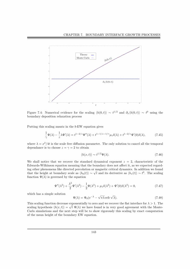
CHAPTER 7. BOUNDARY INTERFACE GROWTH PROCESSES
0.6 0.8 1.0 1.2 1.4 1.6 1.8 2.0
0.7
0.8
0.9
1.0
1.1
1.2
1.3
1.4
t
〈h(0, t)〉
∂x〈h(0, t)〉
Monte Carlo
Theory
Figure 7.4: Numerical evidence for the scaling 〈h(0, t)〉 ∼ t1/2 and ∂x〈h(0, t)〉 ∼ t0 using theboundary deposition relaxation process
Putting this scaling ansatz in the b-EW equation gives
1γ
Ψ(λ)− 1zλΨ′(λ) = t1−2/zΨ′′(λ) + t1−1/z−1/γµ1δ(λ) + t1−2/zΨ′(0)δ(λ), (7.45)
where λ = x2/4t is the scale free diffusion parameter. The only solution to cancel all the temporaldependance is to choose z = γ = 2 to obtain
〈h(x, t)〉 ∼ t1/2Ψ(λ). (7.46)
We shall notice that we recover the standard dynamical exponent z = 2, characteristic of theEdwards-Wilkinson equation meaning that the boundary does not affect it, as we expected regard-ing other phenomena like directed percolation or magnetic critical dynamics. In addition we foundthat the height at boundary scale as 〈h0(t)〉 ∼
√t and its derivative as 〈h1(t)〉 ∼ t0. The scaling
function Ψ(λ) is governed by the equation
Ψ′′(λ2) +λ2
2Ψ′(λ2)− 1
2Ψ(λ2) + µ1δ(λ2) + Ψ′(0)δ(λ2) = 0, (7.47)
which has a simple solutionΨ(λ) = Ψ0(e−λ −
√πλ erfc
√λ). (7.48)
This scaling function decrease exponentially to zero and we recover the flat interface for λ > 1. Thescaling hypothesis 〈h(x, t)〉 =
√t Ψ(λ) we have found is in very good agreement with the Monte-
Carlo simulations and the next step will be to show rigorously this scaling by exact computationof the mean height of the boundary EW equation.
143

CHAPTER 7. BOUNDARY INTERFACE GROWTH PROCESSES
0 1 2 3 4 5
x t-1/2
0.0
0.2
0.4
0.6
<h
(t,x
)> t
-1/2
!(x2/4t)
t=2000t=1500t=1000
Figure 7.5: Mean profile simulated by the deposition-relaxation algorithm. The data are obtainedfor a system of size L = 104 and averaged over 2.105 realizations.
Exact solution
The resolution of the boundary EW equation gives us the exact form of the height
h(x, t) =∫ t
0
dτ∫ ∞
0
du K(x− u, t− τ)[η(u, τ) + δ(u)B(x, t, τ)], (7.49)
where 〈η(x, t)〉 = 〈ζ(x, t)〉 = 0, then the mean solution is given by
〈h(x, t)〉 =∫ t
0
dτ 〈f(x, t, τ)〉∫ ∞
0
du K(x− u, t− τ)δ(u), (7.50)
= 2∫ t
0
dτ K(x, t− τ)〈B(x, t, τ)〉,
which can be written, after some variable changes
〈h(x, t)〉 =t1/2
√4π
∫ ∞
λ
duλ1/2
u3/2
((µ2 − 1)h′
0(t(1− λu−1)) + µ1
)e−u, (7.51)
+1√4π
∫ ∞
λ
du1
u1/2h0(t(1− λu−1))e−u.
144

CHAPTER 7. BOUNDARY INTERFACE GROWTH PROCESSES
Using the expressions of h0(t) and averaging over the noise, we obtain the profile of height afterintegrating over the remaining variable
〈h(x, t)〉 =µ1t
1/2
√4π
Γ(−1/2, λ), (7.52)
where λ = x2/4t. Using the expression of the Gamma function
Γ(−1/2, λ) = 2(e−λ
√λ−√π erfc
√λ), (7.53)
we obtain the final result
〈h(x, t)〉 =µ1√πt1/2
(e−λ −
√πλ erfc
√λ). (7.54)
We can notice that our choice µ1 = 1 help us to recover the correct scaling of the mean height.
7.2.3 Fluctuation of the height of the interface
Monte-Carlo simulations suggest that fluctuations of the interface does not have the exact behaviorwhen we studies a process with or without boundary. For a periodic boundary conditions growthprocess, the width w(x, t) of the interface does not depend on the position x, and scale as tβ beforesaturate at a time tsat ∼ Lz and a value wsat ∼ Lα. This regime is reach when the correlationlength ξ(t) of the interface becomes equal to the size L of the system, after that the process becomesstationary. This scaling informations will be very useful in order to analyze what happens whenwe add a fix boundary in our systems. Simulations seems to confirm that exponents are the sameclose or far away from the boundary, but a crossover between two regimes appears on a time tccharacterized by a anomal fluctuation of the interface. The new scaling is now quit different fromthe periodic case, because w(x, t) become x-dependent and some corrections appears. The widthof the interface changes at a time tc from a standard bulk behavior to a surface behavior whenthe correlation length of the systems ξ(t) = x , where x is the point where we measure the width.Consequently, this new regime appears at a time tc ∼ xz and at a value wc ∼ xα. The space-timewidth w(t, x) is given by
w2(t, x) = C(t, t, x, x) = 〈(h(t, x)− 〈h(t, x)〉)2〉, (7.55)
where, using the change of variable v = 1/(4u) in (7.39),
h(t, x)− 〈h(t, x)〉 =1√π
∫ ∞
λ
e−v
√vζ(t− λt/v, 0) + ζ(t, x). (7.56)
w2(t, x) can be written as the sum of three terms,
w2(t, x) =3∑
i=1
w2i (t, x), (7.57)
145

CHAPTER 7. BOUNDARY INTERFACE GROWTH PROCESSES
10-2
10-1
100
101
tx-2
0.2
0.4
0.6
0.8
1.0
1.2
1.4
1.6
2.0
w(t
,x)
x
x=10
x=20
x=50
t1/4
tx−2
w(t,x
)x−1/2
wcrx−1/2cr
t crx−2
cr
Figure 7.6: Width w(x, t) simulated by the deposition-relaxation algorithm, we notice a clearvariation relative to the standard scaling. The data are obtained for a system of size L = 104 andaveraged over 2.105 realizations.
using the expression of the two-point correlation function between the modified random noise(7.35), we found
w21(t, x) =
1π
∫ ∞
λ
∫ ∞
λ
dv dv′ exp(−v − v′)√vv′
〈ζ(t− tλ/v, 0)ζ(t− tλ/v′, 0)〉 (7.58)
=T√tλ
2π3/2
∫ ∞
1
dv∫ ∞
1
dv′ exp(−λv − λv′)vv′
{√2vv′ − v − v′ −
√|v − v′|
}
= T√t
[√λ
πEi(2λ)− (
√2− 1)
√λ erfc2 λ− 1√
2πe−λ erfc
√λ
],
where Ei(x) =∫∞
−xdu u−1e−u is the exponential integral,
w22(t, x) =
2√π
∫ ∞
λ
dve−v
√v〈ζ(t− tλ/v, 0)ζ(t, x)〉 (7.59)
=T√tλ
π
∫ ∞
1
dve−λv
v
∫ v
1
du√1 + u
[1 + erf
(√(u− 1)λvu(1 + u)
)]exp
(− λv
1 + u
),
146

CHAPTER 7. BOUNDARY INTERFACE GROWTH PROCESSES
and
w23(t, x) = 〈ζ2(t, x)〉 =
T√t√
8π
∫ 1
0
dτ√τ
[1 + erf
(√2λτ
)](7.60)
=T√t
π√λ{√πλ
2− λγ − λ log(2) + 2λ− λ log(λ) +
23λ2
3F3(1, 1,32
; 2, 2,52
;−2λ)}.
where 3F3(1, 1, 32 ; 2, 2, 5
2 ;−2λ) is a generalized hypergeometric function. Then the width can beexpressed in the form w(t, x) =
√Tt1/4Φw(λ). The serie-expansion for λ≪ 1 gives for each term
w(t
,x)t
-1/4
0.7
0.75
0.8
0.85
0.9
0.95
1
4t/x2
10−2 10−1 100 101 102 103
x=2x=4x=6x=8x=10x=15x=20x=30x=40x=60x=80x=100
Φw
Figure 7.7: Effective correction to the exponent β = 1/4. The width scale as w ∼ t1/4 for short andlong time, but a notable correction appears between the two regimes characterized by an effectiveexponent βeff ≈ 0.31.
w21(t, x) ≃ T
√t
(1√2π−[√
2π
+
√2− 12
− 1π
(γ + log(2λ))]√
λ+3√
2− 42√π
λ+O(λ3/2))
w22(t, x) ≃ T
√t
[2√2π
+
√λ
π
(π2
8+π
2− 4√
2 + γ + γ log(2) +√
2 log(3 + 2√
2)) √
λ log(λ)π
[1 + log(2)] +O(λ)
]
w23(t, x) ≃ T
√t
(1√2π
+−γ + 2− log(2λ)
π
√λ+O(λ3/2)
).
This sum of this three terms are compared to the numerical simulations on the Fig. 7.7 and arather good match is found, specially out of the region of small λ.
147

CHAPTER 7. BOUNDARY INTERFACE GROWTH PROCESSES
2-times correlations
Two-time quantities have been shown in many circumstances to yield useful insights into the dy-namical behavior of systems far from equilibrium. Of special interest are space and time dependentfunctions as for example the space-time response R(t, s, x, y) or the height-height space-time corre-lation C(t, s, x, y), which are both defined in the same way as for the magnetic systems consideredbefore
C(t, s, x, y) = 〈h(t, x)h(s, y)〉 − 〈h(t, x)〉〈h(s, y)〉, (7.61)
where the brackets indicate an average over the realization of the noise. In general, withoutassuming any space-time translation, C can always be written as C(t+ s, t− s, x+ y, x− y). Thespace-time response, defined by
R(t, s, x, y) = limj→0
δ〈h(t, x)〉δj(s, y)
, (7.62)
measures the response of the interface at time t and position x to a small perturbation j(s, y) atan earlier time s and at a different position y. For reasons of causality we have t > s. At the levelof the Langevin equation the perturbation enters through the addition of j to the right hand side.In our semi-infinite model, spatial translation invariance in the direction parallel to the interfaceis broken, we have in general
C(t, s, x, y) = C(t− s, t+ s, x− y, x+ y), (7.63)
R(t, s, x, y) = R(t− s, x− y, x+ y).
The response function depends only on t − s because of causality of the response. The auto-correlation and auto-response functions are then defined by
C(t, s) = C(t− s, x− y = 0, x), (7.64)
R(t, s) = R(t− s, x− y = 0, x).
It is well known that the systems discussed here present a simple dynamical scaling behavior inthe standard infinite model. For the two-time quantities one expects the same scaling behavior.For the auto-response and the autocorrelation functions we expect the scaling forms
C(t, s, x) ∼ s−bFC(|x|zs−1, ts−1), (7.65)
R(t, s, x) ∼ s−1−aFR(|x|zs−1, ts−1).
For the auto-response and the auto-correlation functions we expect the scaling forms which definesthe non-equilibrium exponents a and b. One ends up with the scaling relation b = −2α/z, whichrelates b to the known exponents α and z. In addition the scaling functions FC and FR define twoadditional exponents λC and λR by their asymptotic behavior. In the next section, we will see byexact computation if the scaling hypothesis above is correct, and how the two functions FR andFR looks like and how are they related to infinite scaling.
Scaling of correlation functions
The 2-space time correlation function is defined as
C(t, s, x, y) =⟨(h(t, x)− 〈h(t, x)〉)(h(s, y)− 〈h(s, y)〉)
⟩. (7.66)
148
CHAPTER 7. BOUNDARY INTERFACE GROWTH PROCESSES
The computation for the EW equation is rather tedious and not relevant for the understanding,we just write the solution and explore the consequences. The 2-space-time correlation function canbe written as
C(t, s, x, y) = C(t− s, t+ s)∞ΨC
( x− y√4(t− s)
,x+ y√4(t+ s)
,x+ y√4(t− s)
,x− y√4(t+ s)
)
∼ s−bFC
( ts
)ΨasymptC
(x− y√s,x+ y√
s
). (7.67)
The auto-correlation function then reads
C(t, s, 0, x) := C(t, s, x) = C∞(t− s, t+ s)ΨC
( ts,
x√4(t− s)
,x√
4(t+ s)
)(7.68)
∼ s−bFC
( ts
)ΨasymptC
( ts,x
s1/z
),
where
C∞(t− s, t+ s) = T (√t+ s−
√t− s). (7.69)
This quantity C∞(t− s, t+ s) is the exact expression for 2-space-time correlation function in EWequation with periodic boundary conditions as we except.
Scaling of the response function
The space-time response, measures the response of the interface at time t and position x to a smallperturbation j(y, s) at an earlier time s and at a different position y. For reasons of causality wehave t > s. At the level of the Langevin equation the perturbation enters through the addition ofj to the right hand side. The response function, which results from a perturbation in the flux, canbe viewed as the response of the system to the noise itself
R(x, y, t, s) = limj→0
δ〈h(x, t)〉δj(y, s)
=⟨δh(x, t)δη(y, s)
⟩. (7.70)
In order to compute the response of the interface to a small perturbation we add the term j(x, t)to the right-hand side of the Langevin equation and then go to reciprocal space. In the infiniteEW case the solution of the resulting equation is
h(k, t) = e−νk2t
∫ t
0
dt e−νk2t′(η(k, t′) + j(k, t′)). (7.71)
Taking the functional derivative of and transforming back to real space yields the result
R(t, s,x− y) =(t− s)−d/2
(2√πν)d
exp−(x− y)2
4ν(t− s) .
In dimension d = 1, it gives
R(t, s, x− y) = R(t− s, x− y) = θ(t− s) (t− s)−1/2
(2√πν)
exp−(x− y)2
4ν(t− s)
149

CHAPTER 7. BOUNDARY INTERFACE GROWTH PROCESSES
The solution of the boundary EW equation with ν = 1 and µ2 = 1 is
h(x, t) = ζ(x, t) +∫ t
0
dτ1√
4π(t− τ)
((µ1 + h0(τ)
x
2(t− τ)
)e
−x2
4(t−τ) . (7.72)
where ζ(x, t) is a convolution of the noise η(x, t) with the heat kernel
ζ(x, t) =∫ t
0
dτ√4π(t− τ)
∫ ∞
0
duÊη(u, τ) exp−(x− u)2
4(t− τ)
=∫ t
0
∫ ∞
0
dτ du K(x− u, t− τ)η(u, τ).
where we have defined the heat kernel by
K(x, t) :=exp
(−x2/4t
)√
4πt, (7.73)
Putting all together, we find
R(t, s, x, y) = θ(t− s)K(x− y, t− s) + θ(t− s)∫ t−s
0
dτ√4π(t− s− τ)
x
t− s− τ e− x2
4(t−s−τ)− y2
4τ
= θ(t− s)K(x− y, t− s) + θ(t− s)K(x+ y, t+ s) (7.74)
=θ(t− s)√4π(t− s)
exp−(x− y)2
4(t− s) +θ(t− s)√4π(t− s)
exp−(x+ y)2
4(t− s) .
Assuming t > s, one have
R(t, s, x, y) = R(t− s, x− y, x+ y) (7.75)
= R∞(t− s)ΨR
( x− y(t− s)1/z
,x+ y
(t− s)1/2
)
∼ s−1/2FR
( ts
)ΨasymptR
(x− ys1/2
,x+ y
s1/2
)
We can choose x = y, and we obtain the auto-response function
R(t, s, x) =1√
4π(t− s)
(1 + exp
−4x2
4(t− s))
(7.76)
∼ s−1/2FR
( ts
)ΨasymptR
( ts,x√s
)
∼ s−1/2FR
( ts
)ΦasymptR
( x√s
),
where FR(u) ∼ u−λR/z is the same scaling function as the infinite EW equation. Here we notice ascaling relation, since in the infinite EW case the auto-response is
R∞(t− s) =1√
4π(t− s)∼ s−a−1FR
( ts
),
150
CHAPTER 7. BOUNDARY INTERFACE GROWTH PROCESSES
then the auto-response (x = y) function reads
R(t, s, x) = R∞(t− s)ΨR
( x√t− s
)∼ s−a−1FR
( ts
)ΨasymptR
( ts,x√s
)
The auto-response function does depend only on the time difference R(t, s, x) = R(t − s, x) andnot on t + s as in the correlation case C(t, s, x) = C(t + s, t − s, x), this difference comes fromthe causality nature of the response function. The scaling function ΨR interpolates between thesurface and the bulk and behaves as ΨR(∞) ∼ ΨR(0) ∼ cst.
Summary of relations
Generally speaking, we can write relations for quantities close to the boundary as the product ofthe same quantities on the bulk times scaling functions which interpolate between two regimes.We will not show here the explicit forms of the scaling functions for correlations for the sake ofclarity. This scaling behaviors of the auto-response and auto-correlations seem to be similar tothose of the width of the interface
t−1/γ〈h(t, x)〉 = 〈h(t, x)〉∞Ψh
( x
t1/z
)∼ cst Ψasympt
w
( x
t1/z
)(7.77)
w(t, x) = w∞(t)Ψw
( x
t1/z
)∼ tβ Ψasympt
w
( x
t1/z
)
C(t, s, x) = C∞(t− s, t+ s)ΨC
( x
(t+ s)1/z,
x
(t− s)1/z
)∼ s−bFC
( ts
)ΨasymptC
( ts,x
s1/z
)
R(t, s, x) = R∞(t− s)ΨR
( x
(t− s)1/z
)∼ s−1−aFR
( ts
)ΨasymptR
( ts,x
s1/z
)
to compare to the standard infinite scaling
〈h(t, x)〉∞ ∼ cst (7.78)
w∞(t) ∼ tβ
C∞(t− s, t+ s) ∼ s−bFC(ts−1)
R∞(t− s) ∼ s−1−aFR(ts−1),
where FC,R(u) ∼ u−λC,R/z in the asymptotic limit. The infinite label refers to the scaling of theinfinite equation and to the scaling limit x/
√s → ∞ as well, because we recover the standard
behavior for short time or/and large distance. One define FR,C such that
C(t, s, x) ∼ s−bFC
( ts
)ΨasymptC
( ts,x
s1/z
)∼ s−bFC
( ts
)ΦasymptC
( x
s1/z
)(7.79)
R(t, s, x) ∼ s−1−aFR
( ts
)ΨasymptR
( ts,x
s1/z
)∼ s−1−aFR
( ts
)ΦasymptR
( x
s1/z
). (7.80)
7.3 Boundary KPZ equation
In this part, we want to continue the analysis of the growth of an interface close to a boundary inthe case where the microscopic process belongs to the KPZ equation. We will use again the samemachinery to derive the continuous equation for the height and study some of the properties usinga combination of numerical simulations and scaling calculations.
151

CHAPTER 7. BOUNDARY INTERFACE GROWTH PROCESSES
7.3.1 Introduction and definition of the problem
It is very simple to add a boundary in the Kim-Kosterlitz process, we just need to take a semi-infinite lattice i = 1, 2, 3, ... and just precise the rates to impose to the first site i = 1. In the
t = 0
t = 1 t = 1t = 1 t = 2 t = 2 t = 2
t = 3
t = 3 t = 3t = 4
t = 4 t = 4
t = 5
t = 5 t = 5
h(x, t)
BOUNDARY
x
Figure 7.8: Kim-Kosterlitz algorithm with a boundary on a semi-infinite (i = 1, 2, 3...) substrate.The initial state at t = 0 is the white flat interface, then a fixed (3 in the figure) number of particlescan reached the substrate if the condition |hi±1 − hi|ša is fulfilled for i > 1 and |h2 − h1|ša for thesite i = 1, at each time (t = 1 red particles, t = 2 blue particles...).
bulk i 6= 1 we use the same algorithm than in the standard periodic process, and at the origin,we just impose h0 > h1 such that we always have the condition in the left side of the wall, and aparticle is dropped in i = 1 if the condition |h1−h2|ša is fulfilled on the right side. In that case theboundary acts like a source of particle. In this process, we can argue that there is less restrictionin the boundary than in the bulk. For all the site but i = 1 the equation in unchanged
dhi>1
dt= Γa ω
(0)i + ηi(t), (7.81)
= Γa θi+1,iθi−1,i + ηi(t), (7.82)
and the modification for the site i = 1 is simply
dh1
dt= Γa θ21(1− ǫ) + η1(t) (7.83)
= Γa ω(0)1 + ηi(t), (7.84)
where ω(0)1 is the modified transition rate. Now we want to make clear the difference with the i > 1
case so we write the previous equation as
dh1
dt= Γa
(ω
(0)1 + ∆ω
(0)1
)+ ηi(t), (7.85)
where we define ∆ω(0)1 = ω
(0)1 −ω
(0)1 in such way that we can write down an equation for i = 1, 2, 3...
using δij = 1 if i = j and 0 else
dhidt
= Γa(ω
(0)i + ∆ω
(0)i δi,1
)+ ηi(t). (7.86)
152

CHAPTER 7. BOUNDARY INTERFACE GROWTH PROCESSES
7.3.2 KPZ equation with a boundary
As for the EW case the equation is exactly the same for every i > 1 plus a correction term whichacts locally on the boundary. Explicitely ∆ω
(0)1 = ω
(0)1 −ω
(0)1 = θ21(1− ǫ− θ01) After going to the
limit a→ 0, we end up with the same form as for the EW case
∂h
∂t= ν
∂2h
∂x2+ λ
(∂h
∂x
)2
+ ν(
µ1 + µ2h1(t))
δ(x) + η(x, t). (7.87)
where h1(t) =: ∂h(x,t)∂x |x=0. The following result is exactly the KPZ equation plus the boundary
term. As for the EW case, we will suppose µ2 = 1 and then fit the numerics with the parametersof the equation.
7.3.3 Scaling hypothesis and numerical results
This scaling calculation will be useful in order to have informations about the shape of the solutionclose to the boundary and about the evolution of correlations in the process. In the following, weshall proceed to the same analysis as we have done for the linear case. We suppose an asymptoticscaling law for the mean profile
〈h(x, t)〉 ∼ t1/γΨ(x/ξ(t) , (7.88)
where Ψ(u) is a scaling function to determine, which is constant for u = 0 and has to decrease tozero for time bigger t1/z. The same kind of scaling function can be written for the derivative ofthe profile,
∂x〈h(x, t)〉 =t1/γ
ξ(t)∂uΨ(u) ∼ tρ Φ(x/ξ(t)), (7.89)
with ξ(t) scale identically in the two functions Ψ(u) and Φ(u), and ρ = 1/γ − 1/z
θ(t) = ∂x〈h(x, t)〉x=0, (7.90)
scale as θ(t) ∼ tρ. Those two scaling hypothesis should be valid no matter what kind of growthprocess we look at, hence the mean profile of boundary MH or EW equation (exact solution) takesalso this scaling form
〈h0(t)〉 ∼ t1/γ (7.91)
〈h1(t)〉 ∼ tρ.
Now let us try to determine phenomenologically the value of these two exponents. Let us startwith the phenomenological boundary KPZ equation
∂h
∂t= ν
∂2h
∂x2+ λ
(∂h
∂x
)2
+ ν(
µ1 + h1(t))
δ(x) + η. (7.92)
In the linear case λ = 0, the exact solution of the model gave us the following scaling law for themean profile 〈h(x, t)〉 ∼ t1/2Ψ(xt−1/2), leading to z = γ = 2. In the KPZ case, we already knowfrom a long time that z = 3/2, let us try to see if this exponent can be found with our scaling.
153
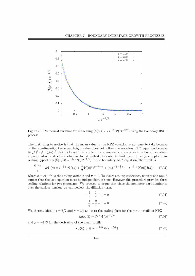
CHAPTER 7. BOUNDARY INTERFACE GROWTH PROCESSES
0
0.1
0.2
0.3
0.4
0.5
0.6
0.7
0.8
0 0.5 1 1.5 2 2.5 3
t = 300t = 350t = 400
x t−2/3
〈h(x,t)〉
t−1/3
Figure 7.9: Numerical evidence for the scaling 〈h(x, t)〉 ∼ t1/3 Ψ(xt−2/3) using the boundary RSOSprocess
The first thing to notice is that the mean value in the KPZ equation is not easy to take becauseof the non-linearity, the mean height value does not follow the noiseless KPZ equation because〈(∂xh)2〉 6= (∂x〈h〉)2. Let us forget this problem for a moment and consider this like a mean-fieldapproximation and let see what we found with it. In order to find z and γ, we just replace ourscaling hypothesis 〈h(x, t)〉 ∼ t1/γ Ψ(xt−1/z) in the boundary KPZ equation, the result is
Ψ(κ)γ
+ κΨ′(κ) = t−2z
+1Ψ′′(κ) +λ
2Ψ′(κ)2t
1γ
− 2z
+1 + (µ1t− 1
z− 1
γ+1 + t−
2z
+1Ψ′(0))δ(κ), (7.93)
where κ = xt−1/z is the scaling variable and ν = 1. To insure scaling invariance, naively one wouldexpect that the last equation must be independent of time. However this procedure provides threescaling relations for two exponents. We proceed to argue that since the nonlinear part dominatesover the surface tension, we can neglect the diffusion term.
−1z− 1γ
+ 1 = 0 (7.94)
1γ− 2z
+ 1 = 0. (7.95)
We thereby obtain z = 3/2 and γ = 3 leading to the scaling form for the mean profile of KPZ
〈h(x, t)〉 ∼ t1/3 Ψ(xt−2/3), (7.96)
and ρ = −1/3 for the derivative of the mean profile
∂x〈h(x, t)〉 ∼ t−1/3 Φ(xt−2/3). (7.97)
154
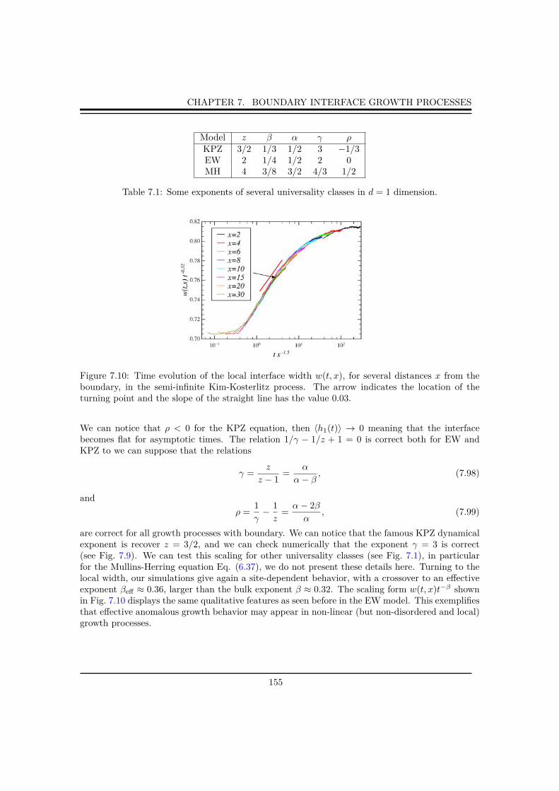
CHAPTER 7. BOUNDARY INTERFACE GROWTH PROCESSES
Model z β α γ ρKPZ 3/2 1/3 1/2 3 −1/3EW 2 1/4 1/2 2 0MH 4 3/8 3/2 4/3 1/2
Table 7.1: Some exponents of several universality classes in d = 1 dimension.
Figure 7.10: Time evolution of the local interface width w(t, x), for several distances x from theboundary, in the semi-infinite Kim-Kosterlitz process. The arrow indicates the location of theturning point and the slope of the straight line has the value 0.03.
We can notice that ρ < 0 for the KPZ equation, then 〈h1(t)〉 → 0 meaning that the interfacebecomes flat for asymptotic times. The relation 1/γ − 1/z + 1 = 0 is correct both for EW andKPZ to we can suppose that the relations
γ =z
z − 1=
α
α− β , (7.98)
andρ =
1γ− 1z
=α− 2βα
, (7.99)
are correct for all growth processes with boundary. We can notice that the famous KPZ dynamicalexponent is recover z = 3/2, and we can check numerically that the exponent γ = 3 is correct(see Fig. 7.9). We can test this scaling for other universality classes (see Fig. 7.1), in particularfor the Mullins-Herring equation Eq. (6.37), we do not present these details here. Turning to thelocal width, our simulations give again a site-dependent behavior, with a crossover to an effectiveexponent βeff ≈ 0.36, larger than the bulk exponent β ≈ 0.32. The scaling form w(t, x)t−β shownin Fig. 7.10 displays the same qualitative features as seen before in the EW model. This exemplifiesthat effective anomalous growth behavior may appear in non-linear (but non-disordered and local)growth processes.
155

CHAPTER 7. BOUNDARY INTERFACE GROWTH PROCESSES
7.4 Conclusions
In summary, in several semi-infinite lattice models of interface growth, the simple boundary con-dition h0(t) ≥ h1(t) on the heights on the two sites nearest to the boundary not only leads to non-constant and non-stationary height profiles but also to site-dependent roughness profiles. Thereexists a large range of times where effective growth exponents β with values clearly larger thanin deep in the bulk can be identified, in qualitative analogy with known experiments on growinginterfaces [158, 130, 153, 84, 130, 52]. However, since we have concentrated on models defined inthe simple geometry of a semi-infinite line with a single boundary, a quantitative comparison withthe experiments, carried out on faceted growing surfaces with many interacting interfaces, maybe premature. For non-disordered models with local interactions, the truly asymptotic growthexponents return to the simple bulk values, as predicted by the rg [150]. The unexpectedly com-plex behavior at intermediate times is only seen if appropriate boundary terms are included in theLangevin equation describing the growth process. The non-stationary height profiles are reminis-cent of behavior found in systems undergoing physical ageing, which is known to occur in modelsdescribing interface growth [94]. Our results were obtained through the exact solution of the semi-infinite EW class and through extensive Monte-Carlo simulations of both profiles and widths inthe EW and KPZ models. A scaling relation for the surface profile exponent γ was proposed andis in agreement with all presently known model results.
156
CHAPTER 8. RÉSUMÉ EN FRANÇAIS DE LA PARTIE II
CHAPTER8Résumé en français de la partie II
Propriétés critiques d’interfaces en croissance
Les processus de croissance d’interfaces sont des phénomènes dynamiques qui peuvent être décritspar des équations de Langevin pour un paramètre d’ordre (dans ce cas la hauteur h(x, t)). Con-trairement aux phénomènes critiques d’équilibres, il n’y a pas de réelles transitions de phases dansces modèles mais un comportement critique de fluctuations de l’interface.
Dynamique d’interface et propriétés d’échelle
Un des cas le plus simple d’equation de croissance d’interface dû à un processus de deposition-relaxation, est l’équation de Edwards-Wilkinson
∂th(x, t) = ν∂2xh(x, t) + η(x, t), (8.1)
ou η est un bruit blanc gaussien
〈η(x, t)〉 = 0 (8.2)
〈η(x, t)η(x′, t′)〉 = 2Dδ(x− x′)δ(t− t′). (8.3)
Cette équation est la limite continue de nombreux processus microscopiques et sa résolution esttrès simple dû à la linéarité de l’équation. La résolution conduit à un ensemble d’exposantscritiques qui caractérisent la classe d’universalité EW. L’hypothèse d’invariance d’échelle est unoutil puissant pour trouver ces exposants très facilement. Dans le cas d’une l’interface fractale,nous redimensionnons la hauteur, et l’espace-temps comme suit
x→ x′ = bx (8.4)
t→ t′ = bzt (8.5)
h→ h′ = bαh, (8.6)
où α, z sont deux exposants qui caractérisent la classe d’universalité du processus. Les propriétésstatistiques de l’interface doivent être inchangés par cette transformation. L’équation EW s’écrit
∂th(x, t)− ν∇2h(x, t) = η(x, t). (8.7)
157
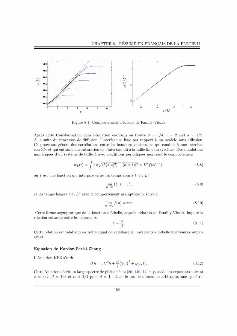
CHAPTER 8. RÉSUMÉ EN FRANÇAIS DE LA PARTIE II
t/Lz
w(t)/Lα
Figure 8.1: Comportement d’échelle de Family-Viczek
Après cette transformation dans l’équation ci-dessus on trouve β = 1/4, z = 2 and α = 1/2.A la suite du processus de diffusion, l’interface se lisse par rapport à un modèle sans diffusion.Ce processus génère des corrélations entre les hauteurs voisines, ce qui conduit à une interfacecorrélée et qui entraîne une saturation de l’interface dû à la taille finie du système. Des simulationsnumériques d’un système de taille L avec conditions périodiques montrent le comportement
wL(t) =∫
dx√〈h(x, t)2〉 − 〈h(x, t)〉2 = Lαf(tL−z), (8.8)
où f est une fonction qui interpole entre les temps courts t << Lz
limu→0
f(u) = uβ , (8.9)
et les temps longs t >> Lz avec le comportement asymptotique suivant
limu→∞
f(u) = cst. (8.10)
Cette forme asymptotique de la fonction d’échelle, appelée relation de Familly-Viczek, impose larelation suivante entre les exposants
z =α
β. (8.11)
Cette relation est valable pour toute équation satisfaisant l’invariance d’échelle mentionnée aupar-avant.
Equation de Kardar-Parisi-Zhang
L’équation KPZ s’écrit∂th = ν∇2h+
µ
2
(∇h)2
+ η(x, t). (8.12)
Cette équation décrit un large spectre de phénomènes [86, 146, 14] et possède les exposants suivantz = 3/2, β = 1/3 et α = 1/2 pour d = 1. Dans le cas de dimension arbitraire, une symétrie
158

CHAPTER 8. RÉSUMÉ EN FRANÇAIS DE LA PARTIE II
particulière est trouvée
h→ h′ = h+ ǫx, (8.13)
x→ x′ = x− µ
2ǫt, (8.14)
t→ t′ = t, (8.15)
où ǫ est un angle infinitesimal. Une des conséquence est la relation α + z = 2 valide en toutedimension.
Croissance d’une interface près d’un bord
Ici nous voulons étudier le comportement d’une interface en présence d’un bord, notre modèle estdécrit par l’équation suivante
∂th(x, t) = ν∂2xh(x, t) + ν
(µ1 + µ2h1(t)
)δ(x) + η(x, t), (8.16)
où h1(t) = ∂xh(x = 0, t) and η est le bruit blanc gaussien. Un ansatz d’échelle peut être postulé
〈h(x, t)〉 ∼ t1/γΨ( x
t1/z
). (8.17)
Ψ(u) est une fonction à déterminer, qui est constante pour u = 0 et décroit pour des tempssupérieurs à t1/z. La seule solution est de choisir z = γ = 2. La forme de la fonction Ψ(λ) peutaussi être déduite et l’on trouve
Ψ(λ) = Ψ0(e−λ −√πλ erfc
√λ). (8.18)
Cette formule est en très bon accord avec les simulations et on peut montrer que cette solutionest exacte. Les simulations Monte-Carlo suggèrent que les fluctuations de l’interface n’ont pas les
0 1 2 3 4 5
x t-1/2
0.0
0.2
0.4
0.6
<h(t
,x)>
t-1
/2
!(x2/4t)
t=2000t=1500t=1000
10-2
10-1
100
101
tx-2
0.2
0.4
0.6
0.8
1.0
1.2
1.4
1.6
2.0
w(t
,x)
x
x=10
x=20
x=50
t1/4
tx−2
w(t,x
)x−1/2
wcrx−1/2cr
t crx−2
cr
Figure 8.2: Gauche: Profil moyen de l’interface. Droite: Fluctuation w(x, t), on remarque un écartsignificatif au comportement usuel
159

CHAPTER 8. RÉSUMÉ EN FRANÇAIS DE LA PARTIE II
mêmes comportements quand on étudie le processus avec ou sans bord. Pour un processus decroissance avec conditions aux limites périodiques, la largeur w(x, t) de l’interface ne dépend pasde la position x et sature pour une valeur wsat ∼ Lα. Ce régime est atteint lorsque la longueurde corrélation ξ(t) de l’interface devient de l’ordre de grandeur de la taille L du système. Lenouveau comportement d’échelle est maintenant assez différent du cas périodique, w(x, t) devientmaintenant fortement dépendant de la position. Le phénomène est explicite sur la figure ci-dessuset les détails sont exposés dans le texte principal. Le système montre un comportement de surfacenon standard et un calcul analytique peut être mis en oeuvre pour expliquer ce phénomène. Uneétude similaire peut être faite pour l’equation KPZ et le même comportement du profil et desfluctuations de l’interface proche du bords est observé.
160

BIBLIOGRAPHY
Bibliography
[1] J. H. Ahrens. Paving the chessboard. Journal of Combinatorial Theory, Series A, 31(3):277–288, 1981.
[2] D. Alberici and P. Contucci. Solution of the Monomer-Dimer Model on Locally Tree-LikeGraphs. Rigorous Results. Communications in Mathematical Physics, pages 1–29, 2013.
[3] F. Alet, Y. Ikhlef, J. L. Jacobsen, G. Misguich, and V. Pasquier. Classical dimers withaligning interactions on the square lattice. Physical Review E, 74(4):041124, 2006.
[4] F. Alet, J. L. Jacobsen, G. Misguich, V. Pasquier, F. Mila, and M. Troyer. Interactingclassical dimers on the square lattice. Physical Review Letters, 94(23):235702, 2005.
[5] N. Allegra. Exact solution of the 2d dimer model: Corner free energy, correlation functionsand combinatorics. arXiv preprint arXiv:1410.4131, 2014.
[6] N. Allegra, J. Dubail, J.-M. Stephan, and J. Viti. Inhomogenous field theory inside the arcticcircle. arXiv preprint arXiv:1512.02872, 2015.
[7] N. Allegra and J.-Y. Fortin. Grassmannian representation of the two-dimensional monomer-dimer model. Physical Review E, 89(6):062107, 2014.
[8] N. Allegra, J.-Y. Fortin, and M. Henkel. Boundary crossover in semi-infinite non-equilibriumgrowth processes. Journal of Statistical Mechanics: Theory and Experiment, 2014(2):P02018,2014.
[9] D. Allison and N. Reshetikhin. Numerical study of the 6-vertex model with domain wallboundary conditions. In Annales de l’institut Fourier, volume 55, pages 1847–1869, 2005.
[10] T. Antal, Z. Rácz, A. Rákos, and G. Schütz. Transport in the xx chain at zero temperature:Emergence of flat magnetization profiles. Physical Review E, 59(5):4912, 1999.
[11] C. T. Asplund and S. G. Avery. Evolution of entanglement entropy in the d1-d5 brane system.Physical Review D, 84(12):124053, 2011.
[12] C. T. Asplund and A. Bernamonti. Mutual information after a local quench in conformalfield theory. Physical Review D, 89(6):066015, 2014.
[13] H. Au-Yang and J. H. H. Perk. Ising correlations at the critical temperature. Physics LettersA, 104(3):131–134, 1984.
[14] A.-L. Barabási and H. E. Stanley. Fractal concepts in surface growth. Cambridge universitypress, 1995.
161

BIBLIOGRAPHY
[15] R. J. Baxter. Dimers on a rectangular lattice. Journal of Mathematical Physics., 9(4):650–654, 1968.
[16] R. J. Baxter. Partition function of the eight-vertex lattice model. Ann. Phys., 70(1):193–228,1972.
[17] R. J. Baxter. Exactly solved models in statistical mechanics. Courier Dover Publications,2007.
[18] A. A. Belavin, A. M. Polyakov, and A. B. Zamolodchikov. Infinite conformal symmetry intwo-dimensional quantum field theory. Nuclear Physics B, 241(2):333–380, 1984.
[19] F. A. Berezin. The Method of second quantization. Academic Press, 1966.
[20] H. Bethe. Zur Theorie der Metalle. Zeitschrift für Physik, 71(3-4):205–226, 1931.
[21] H. Blöte, J. L. Cardy, and M. Nightingale. Conformal invariance, the central charge, anduniversal finite-size amplitudes at criticality. Physical Review Letters, 56(7):742, 1986.
[22] H. Blöte and H. Hilborst. Roughening transitions and the zero-temperature triangular isingantiferromagnet. Journal of Physics A: Mathematical and General, 15(11):L631, 1982.
[23] N. Bogoliubov, A. Pronko, and M. Zvonarev. Boundary correlation functions of the six-vertexmodel. Journal of Physics A: Mathematical and General, 35(27):5525, 2002.
[24] R. Bondesan, J. Dubail, J. L. Jacobsen, and H. Saleur. Conformal boundary state for therectangular geometry. Nuclear Physics B, 862(2):553–575, 2012.
[25] R. Bondesan, J. L. Jacobsen, and H. Saleur. Rectangular amplitudes, conformal blocks, andapplications to loop models. Nuclear Physics B, 867(3):913–949, 2013.
[26] C. Boutillier, J. Bouttier, G. Chapuy, S. Corteel, and S. Ramassamy. Dimers on rail yardgraphs. arXiv preprint arXiv:1504.05176, 2015.
[27] J. Bouttier, M. Bowick, E. Guitter, and M. Jeng. Vacancy localization in the square dimermodel. Physical Review E, 76:041140, Oct 2007.
[28] J. Bouttier, G. Chapuy, and S. Corteel. From aztec diamonds to pyramids: steep tilings.arXiv preprint arXiv:1407.0665, 2014.
[29] J. Brankov. Isomorphism of dimer configurations and spanning trees on finite square lattices.Journal of Mathematical Physics, 36(9):5071–5083, 1995.
[30] P. Calabrese and J. Cardy. Time dependence of correlation functions following a quantumquench. Physical review letters, 96(13):136801, 2006.
[31] P. Calabrese and J. Cardy. Entanglement and correlation functions following a local quench:a conformal field theory approach. Journal of Statistical Mechanics: Theory and Experiment,2007(10):P10004, 2007.
[32] P. Calabrese and J. Cardy. Quantum quenches in extended systems. Journal of StatisticalMechanics: Theory and Experiment, 2007(06):P06008, 2007.
162
BIBLIOGRAPHY
[33] P. Calabrese, C. Hagendorf, and P. Le Doussal. Time evolution of one-dimensional gaplessmodels from a domain wall initial state: stochastic loewner evolution continued? Journal ofStatistical Mechanics: Theory and Experiment, 2008(07):P07013, 2008.
[34] P. Calabrese and P. Le Doussal. Exact solution for the kardar-parisi-zhang equation withflat initial conditions. Physical review letters, 106(25):250603, 2011.
[35] S. Caracciolo, J. L. Jacobsen, H. Saleur, A. D. Sokal, and A. Sportiello. Fermionic fieldtheory for trees and forests. Physical Review Letters, 93(8):080601, 2004.
[36] S. Caracciolo, A. D. Sokal, and A. Sportiello. Grassmann integral representation for spanninghyperforests. Journal of Physics A: Mathematical and Theoretical, 40(46):13799, 2007.
[37] J. L. Cardy. Effect of boundary conditions on the operator content of two-dimensionalconformally invariant theories. Nuclear Physics B, 275(2):200–218, 1986.
[38] J. L. Cardy. Boundary conditions, fusion rules and the Verlinde formula. Nuclear PhysicsB, 324(3):581–596, 1989.
[39] J. L. Cardy and I. Peschel. Finite-size dependence of the free energy in two-dimensionalcritical systems. Nuclear Physics B, 300:377–392, 1988.
[40] S. Chhita and K. Johansson. Domino statistics of the two-periodic aztec diamond. arXivpreprint arXiv:1410.2385, 2014.
[41] A. L.-S. Chua, C. A. Haselwandter, C. Baggio, and D. D. Vvedensky. Langevin equationsfor fluctuating surfaces. Physical Review E, 72(5):051103, 2005.
[42] M. Clusel and J.-Y. Fortin. Boundary field induced first-order transition in the 2D Isingmodel: exact study. J. Phys. A: Mathematical and General, 39(5):995, 2006.
[43] M. Clusel and J.-Y. Fortin. Grassmann techniques applied to classical spin systems. Con-densed Matter Physics, 12(3):463, 2009.
[44] M. Clusel, J.-Y. Fortin, and V. N. Plechko. Alternative description of the 2D Blume-Capel model using Grassmann algebra. Journal of Physics A: Mathematical and Theoretical,41(40):405004, 2008.
[45] H. Cohn, N. Elkies, and J. Propp. Local statistics for random domino tilings of the aztecdiamond. arXiv preprint math/0008243, 2000.
[46] H. Cohn, N. Elkies, J. Propp, et al. Local statistics for random domino tilings of the Aztecdiamond. Duke Mathematical Journal, 85(1):117–166, 1996.
[47] H. Cohn, M. Larsen, and J. Propp. The shape of a typical boxed plane partition. New YorkJ. Math, 4(137):165, 1998.
[48] F. Colomo and A. Pronko. On two-point boundary correlations in the six-vertex model withdomain wall boundary conditions. Journal of Statistical Mechanics: Theory and Experiment,2005(05):P05010, 2005.
[49] F. Colomo and A. Pronko. The arctic circle revisited. Contemporary Mathematics, 458:361,2008.
163

BIBLIOGRAPHY
[50] F. Colomo and A. Pronko. The arctic curve of the domain-wall six-vertex model. Journal ofStatistical Physics, 138(4-5):662–700, 2010.
[51] F. Colomo, A. Pronko, and P. Zinn-Justin. The arctic curve of the domain wall six-vertexmodel in its antiferroelectric regime. Journal of Statistical Mechanics: Theory and Experi-ment, 2010(03):L03002, 2010.
[52] P. Córdoba-Torres, T. Mesquita, I. Bastos, and R. Nogueira. Complex dynamics duringmetal dissolution: From intrinsic to faceted anomalous scaling. Physical review letters,102(5):055504, 2009.
[53] R. Costa-Santos and B. M. McCoy. Dimers and the critical Ising model on lattices of genus> 1. Nuclear Physics B, 623(3):439–473, 2002.
[54] L. F. Cugliandolo, G. Gonnella, and A. Pelizzola. Six vertex model with domain-wall bound-ary conditions in the bethe-peierls approximation. arXiv preprint arXiv:1501.00883, 2014.
[55] K. Damle, D. Dhar, and K. Ramola. Resonating valence bond wave functions and classicalinteracting dimer models. Physical review letters, 108(24):247216, 2012.
[56] P. Di Francesco, D. Sénéchal, and P. Mathieu. Conformal field theory. Springer, 1997.
[57] P. Di Francesco and R. Soto-Garrido. Arctic curves of the octahedron equation. Journal ofPhysics A: Mathematical and Theoretical, 47(28):285204, 2014.
[58] J. Dubail. Conditions aux bords dans des théories conformes non unitaires. PhD thesis,Université Paris 11, 2010.
[59] J. Dubail and J.-M. Stéphan. Universal behavior of a bipartite fidelity at quantum criticality.Journal of Statistical Mechanics: Theory and Experiment, 2011(03):L03002, 2011.
[60] B. A. Dubrovin, A. T. Fomenko, and S. P. Novikov. Modern geometryÑmethods and appli-cations. part i, volume 93 of. Graduate Texts in Mathematics.
[61] B. Duplanticr and F. David. Exact partition functions and correlation functions of multiplehamiltonian walks on the manhattan lattice. Journal of Statistical Physics, 51(3-4):327–434,1988.
[62] S. F. Edwards and D. Wilkinson. The surface statistics of a granular aggregate. In Proceedingsof the Royal Society of London A: Mathematical, Physical and Engineering Sciences, volume381, pages 17–31. The Royal Society, 1982.
[63] N. Elkies, G. Kuperberg, M. Larsen, and J. Propp. Alternating-sign matrices and dominotilings (part i). Journal of Algebraic Combinatorics, 1(2):111–132, 1992.
[64] N. Elkies, G. Kuperberg, M. Larsen, and J. Propp. Alternating-sign matrices and dominotilings (part i). Journal of Algebraic Combinatorics, 1(2):111–132, 1992.
[65] N. Elkies, G. Kuperberg, M. Larsen, and J. Propp. Alternating-sign matrices and dominotilings (part ii). Journal of Algebraic Combinatorics, 1(3):219–234, 1992.
[66] V. Elser. Solution of the dimer problem on a hexagonal lattice with boundary. Journal ofPhysics A: Mathematical and General, 17(7):1509, 1984.
164
BIBLIOGRAPHY
[67] F. Family. Scaling of rough surfaces: effects of surface diffusion. Journal of Physics A:mathematical and general, 19(8):L441, 1986.
[68] P. Fendley, R. Moessner, and S. L. Sondhi. Classical dimers on the triangular lattice. PhysicalReview B, 66(21):214513, 2002.
[69] A. E. Ferdinand. Statistical mechanics of dimers on a quadratic lattice. Journal of Mathe-matical Physics, 8(12):2332–2339, 1967.
[70] P. L. Ferrari and H. Spohn. Random growth models. arXiv preprint arXiv:1003.0881, 2010.
[71] M. E. Fisher. Statistical mechanics of dimers on a plane lattice. Physical. Review, 124(6):1664,1961.
[72] M. E. Fisher and J. Stephenson. Statistical mechanics of dimers on a plane lattice. II. Dimercorrelations and monomers. Physical Review, 132(4):1411, 1963.
[73] J. Fjaerestad. Classical and quantum dimers on the star lattice. Bulletin of the AmericanPhysical Society, 54, 2009.
[74] J. Fjærestad. The 3-edge-colouring problem on the 4–8 and 3–12 lattices. Journal of Statis-tical Mechanics: Theory and Experiment, 2010(01):P01004, 2010.
[75] J. Fjærestad. Dimer and fermionic formulations of a class of colouring problems. Journal ofPhysics A: Mathematical and Theoretical, 45(7):075001, 2012.
[76] P. Flajolet and R. Sedgewick. Analytic combinatorics. Cambridge University Press, 2009.
[77] J.-Y. Fortin and M. Clusel. Second-order critical lines of spin-S Ising models in a splittingfield using Grassmann techniques. Physical Review B, 78(17):172402, 2008.
[78] R. H. Fowler and G. S. Rushbrooke. An attempt to extend the statistical theory of perfectsolutions. Trans. Faraday Soc., 33:1272–1294, 1937.
[79] E. Fradkin. Field theories of condensed matter physics. Cambridge University Press, 2013.
[80] E. Fradkin and L. P. Kadanoff. Disorder variables and para-fermions in two-dimensionalstatistical mechanics. Nuclear Physics B, 170(1):1–15, 1980.
[81] S. Franco, A. Hanany, D. Vegh, B. Wecht, and K. D. Kennaway. Brane dimers and quivergauge theories. Journal of High Energy Physics, 2006(01):096, 2006.
[82] A. Gambassi and P. Calabrese. Quantum quenches as classical critical films. EPL (Euro-physics Letters), 95(6):66007, 2011.
[83] A. Ghosh, D. Dhar, and J. L. Jacobsen. Random trimer tilings. Physical Review E,75(1):011115, 2007.
[84] H. Gong and S. Yim. Study on anomalous scaling exponents for molecular thin film growthusing surface lateral diffusion model. Bulletin of the Korean Chemical Society, 32(7):2237–2242, 2011.
165

BIBLIOGRAPHY
[85] T. Gueudré and P. Le Doussal. Directed polymer near a hard wall and kpz equation in thehalf-space. EPL (Europhysics Letters), 100(2):26006, 2012.
[86] T. Halpin-Healy and Y.-C. Zhang. Kinetic roughening phenomena, stochastic growth, di-rected polymers and all that. aspects of multidisciplinary statistical mechanics. Physicsreports, 254(4):215–414, 1995.
[87] A. Hanany and K. D. Kennaway. Dimer models and toric diagrams. arXiv preprint hep-th/0503149, 2005.
[88] R. Hayn and V. N. Plechko. Grassmann variables and exact solutions for two-dimensionaldimer models. Physics of Atomic Nuclei, 61:1972–1977, 1998.
[89] O. J. Heilmann and E. H. Lieb. Monomers and dimers. Physical Review Letters, 24:1412–1414, 1970.
[90] O. J. Heilmann and E. H. Lieb. Theory of monomer-dimer systems. Communication inMathematical Physics, 25(3):190–232, 1972. reprinted in: Statistical Mechanics, edited by B.Nachtergaele, J. P. Solovej, and J. Yngvason, Springer (2004), pp. 45-87.
[91] H. Helfgott. Edge effects on local statistics in lattice dimers: a study of the Aztec diamond(finite case). PhD thesis, Citeseer, 1998.
[92] M. Henkel. Conformal invariance and critical phenomena. Springer, 1999.
[93] M. Henkel. Conformal invariance and critical phenomena. Springer Science & BusinessMedia, 2013.
[94] M. Henkel and M. Pleimling. Non-equilibrium phase transitions, volume 2: Ageing anddynamical scaling far from equilibrium (theoretical and mathematical physics), 2010.
[95] C. L. Henley. Relaxation time for a dimer covering with height representation. Journal ofStatistical Physics, 89(3-4):483–507, 1997.
[96] F. Iglói, I. Peschel, and L. Turban. Inhomogeneous systems with unusual critical behaviour.Advances in Physics, 42(6):683–740, 1993.
[97] L. Ioffe and A. Larkin. Superconductivity in the liquid-dimer valence-bond state. PhysicalReview B, 40(10):6941, 1989.
[98] C. Itzykson and J.-M. Drouffe. Statistical Field Theory: Volume 1, From brownian motionto renormalization and lattice gauge theory. Cambridge University Press, 1991.
[99] C. Itzykson, H. Saleur, and J.-B. Zuber. Conformal invariance of nonunitary 2d-models. EPL(Europhysics Letters), 2(2):91, 1986.
[100] A. G. Izergin. Partition function of the six-vertex model in a finite volume. In Soviet PhysicsDoklady, volume 32, page 878, 1987.
[101] A. G. Izergin, D. A. Coker, and V. E. Korepin. Determinant formula for the six-vertex model.Journal of Physics A: Mathematical and General, 25(16):4315, 1992.
166
BIBLIOGRAPHY
[102] N. S. Izmailian and R. Kenna. Dimer model on a triangular lattice. Physical Review E,84(2):021107, 2011.
[103] N. S. Izmailian, R. Kenna, W. Guo, and X. Wu. Exact finite-size corrections and corner freeenergies for the c = −2 universality class. Nuclear Physics B, 884:157–171, 2014.
[104] N. S. Izmailian, K. Oganesyan, and C.-K. Hu. Exact finite-size corrections of the free energyfor the square lattice dimer model under different boundary conditions. Physical Review E,67(6):066114, 2003.
[105] N. S. Izmailian, K. Oganesyan, M.-C. Wu, and C.-K. Hu. Finite-size corrections and scalingfor the triangular lattice dimer model with periodic boundary conditions. Physical ReviewE, 73(1):016128, 2006.
[106] N. S. Izmailian, V. B. Priezzhev, P. Ruelle, and C.-K. Hu. Logarithmic conformal field theoryand boundary effects in the dimer model. Physical Review Letters, 95:260602, Dec 2005.
[107] J. Jacobsen. AlgŔbre, intŐgralitŐ et modŔles exactement solubles (cours de m2 de physiquethŐorique), 2013.
[108] J. Jacobsen and P. Zinn-Justin. Algebraic bethe ansatz for the fpl2 model. Journal of PhysicsA: Mathematical and General, 37(29):7213, 2004.
[109] J. L. Jacobsen. Bulk, surface and corner free-energy series for the chromatic polynomialon the square and triangular lattices. Journal of Physics A: Mathematical and Theoretical,43(31):315002, 2010.
[110] J. L. Jacobsen and J. Kondev. Field theory of compact polymers on the square lattice.Nuclear Physics B, 532(3):635–688, 1998.
[111] M. Jeng, M. J. Bowick, W. Krauth, J. Schwarz, and X. Xing. Vacancy diffusion in thetriangular-lattice dimer model. Physical Review E, 78(2):021112, 2008.
[112] M. R. Jerrum. Two-dimensional monomer-dimer systems are computationally intractable.Journal of Statistical Physics, 48(1-2):121–134, 1987. Erratum-ibid 59, 1087-1088 (1990).
[113] W. Jockusch, J. Propp, and P. Shor. Random domino tilings and the arctic circle theorem.arXiv preprint math/9801068, 1998.
[114] K. Johansson. The arctic circle boundary and the airy process. Annals of probability, pages1–30, 2005.
[115] K. Johansson. The arctic circle boundary and the airy process. Annals of probability, pages1–30, 2005.
[116] K. Johansson and E. Nordenstam. Eigenvalues of gue minors. Electron. J. Probab,11(50):1342–1371, 2006.
[117] P. E. John and H. Sachs. On a strange observation in the theory of the dimer problem.Discrete Mathematics, 216(1):211–219, 2000.
[118] L. P. Kadanoff and H. Ceva. Determination of an operator algebra for the two-dimensionalIsing model. Physical Review B, 3(11):3918, 1971.
167
BIBLIOGRAPHY
[119] M. Kardar, G. Parisi, and Y.-C. Zhang. Dynamic scaling of growing interfaces. PhysicalReview Letters, 56(9):889, 1986.
[120] P. W. Kasteleyn. The statistics of dimers on a lattice: I. the number of dimer arrangementson a quadratic lattice. Physica, 27(12):1209–1225, 1961.
[121] P. W. Kasteleyn. Dimer statistics and phase transitions. Journal of Mathematical Physics,4:287, 1963.
[122] B. Kaufman. Crystal statistics. II. Partition function evaluated by spinor analysis. PhysicalReview, 76(8):1232, 1949.
[123] B. Kaufman and L. Onsager. Crystal statistics. III. Short-range order in a binary Isinglattice. Physical Review, 76(8):1244, 1949.
[124] D. Kennes, V. Meden, and R. Vasseur. Universal quench dynamics of interacting quantumimpurity systems. Physical Review B, 90(11):115101, 2014.
[125] C. Kenyon, D. Randall, and A. Sinclair. Approximating the number of monomer-dimercoverings of a lattice. Journal of Statistical Physics, 83(3-4):637–659, 1996.
[126] R. Kenyon. Conformal invariance of domino tiling. Annals of probability, pages 759–795,2000.
[127] R. Kenyon. Dominos and the gaussian free field. Annals of probability, pages 1128–1137,2001.
[128] R. Kenyon. Lectures on dimers. arXiv preprint arXiv:0910.3129, 2009.
[129] R. Kenyon, A. Okounkov, and S. Sheffield. Dimers and amoebae. Annals of mathematics,pages 1019–1056, 2006.
[130] J. Kim, N. Lim, C. R. Park, and S. Yim. Growth dynamics of znpc and tiopc thin films:Effect of crystallinity on anomalous scaling behavior. Surface Science, 604(13):1143–1147,2010.
[131] J. M. Kim and J. Kosterlitz. Growth in a restricted solid-on-solid model. Physical reviewletters, 62(19):2289, 1989.
[132] P. Kleban and I. Vassileva. Free energy of rectangular domains at criticality. Journal ofPhysics A: Mathematical and General, 24(14):3407, 1991.
[133] P. Kleban and I. Vassileva. Domain boundary energies in finite regions at 2d criticality viaconformal field theory. Journal of Physics A: Mathematical and General, 25(22):5779, 1992.
[134] J. Kondev and C. L. Henley. Four-coloring model on the square lattice: A critical groundstate. Physical Review B, 52(9):6628, 1995.
[135] J. Kondev and J. L. Jacobsen. Conformational entropy of compact polymers. Physical ReviewLetters, 81(14):2922, 1998.
[136] Y. Kong. Logarithmic corrections in the free energy of monomer-dimer model on planelattices with free boundaries. Physical Review E, 74(1):011102, 2006.
168
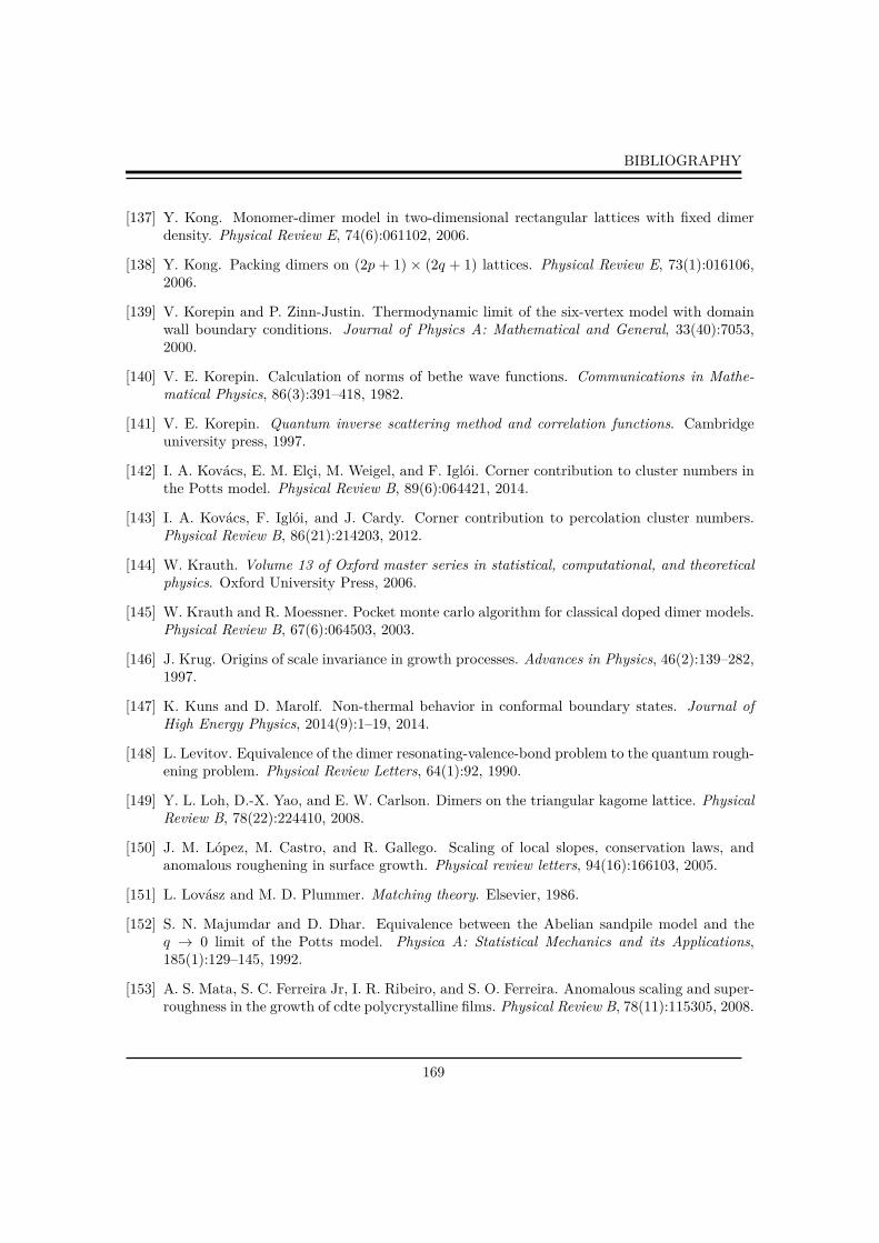
BIBLIOGRAPHY
[137] Y. Kong. Monomer-dimer model in two-dimensional rectangular lattices with fixed dimerdensity. Physical Review E, 74(6):061102, 2006.
[138] Y. Kong. Packing dimers on (2p + 1) × (2q + 1) lattices. Physical Review E, 73(1):016106,2006.
[139] V. Korepin and P. Zinn-Justin. Thermodynamic limit of the six-vertex model with domainwall boundary conditions. Journal of Physics A: Mathematical and General, 33(40):7053,2000.
[140] V. E. Korepin. Calculation of norms of bethe wave functions. Communications in Mathe-matical Physics, 86(3):391–418, 1982.
[141] V. E. Korepin. Quantum inverse scattering method and correlation functions. Cambridgeuniversity press, 1997.
[142] I. A. Kovács, E. M. Elçi, M. Weigel, and F. Iglói. Corner contribution to cluster numbers inthe Potts model. Physical Review B, 89(6):064421, 2014.
[143] I. A. Kovács, F. Iglói, and J. Cardy. Corner contribution to percolation cluster numbers.Physical Review B, 86(21):214203, 2012.
[144] W. Krauth. Volume 13 of Oxford master series in statistical, computational, and theoreticalphysics. Oxford University Press, 2006.
[145] W. Krauth and R. Moessner. Pocket monte carlo algorithm for classical doped dimer models.Physical Review B, 67(6):064503, 2003.
[146] J. Krug. Origins of scale invariance in growth processes. Advances in Physics, 46(2):139–282,1997.
[147] K. Kuns and D. Marolf. Non-thermal behavior in conformal boundary states. Journal ofHigh Energy Physics, 2014(9):1–19, 2014.
[148] L. Levitov. Equivalence of the dimer resonating-valence-bond problem to the quantum rough-ening problem. Physical Review Letters, 64(1):92, 1990.
[149] Y. L. Loh, D.-X. Yao, and E. W. Carlson. Dimers on the triangular kagome lattice. PhysicalReview B, 78(22):224410, 2008.
[150] J. M. López, M. Castro, and R. Gallego. Scaling of local slopes, conservation laws, andanomalous roughening in surface growth. Physical review letters, 94(16):166103, 2005.
[151] L. Lovász and M. D. Plummer. Matching theory. Elsevier, 1986.
[152] S. N. Majumdar and D. Dhar. Equivalence between the Abelian sandpile model and theq → 0 limit of the Potts model. Physica A: Statistical Mechanics and its Applications,185(1):129–145, 1992.
[153] A. S. Mata, S. C. Ferreira Jr, I. R. Ribeiro, and S. O. Ferreira. Anomalous scaling and super-roughness in the growth of cdte polycrystalline films. Physical Review B, 78(11):115305, 2008.
169

BIBLIOGRAPHY
[154] B. M. McCoy and T. T. Wu. The Two-Dimensional Ising Model. Harvard University Press,1973.
[155] R. Merris. Laplacian matrices of graphs: a survey. Linear algebra and its applications,197:143–176, 1994.
[156] R. Moessner and K. S. Raman. Quantum dimer models. In Introduction to FrustratedMagnetism, pages 437–479. Springer, 2011.
[157] M. Nakahara. Geometry, topology and physics. CRC Press, 2003.
[158] F. S. Nascimento, S. C. Ferreira, and S. O. Ferreira. Faceted anomalous scaling in theepitaxial growth of semiconductor films. EPL (Europhysics Letters), 94(6):68002, 2011.
[159] B. Nienhuis. Coulomb gas formulations of two-dimensional phase transitions. In PhaseTransitions and Critical Phenomena, volume 11. Academic press, 1987.
[160] B. Nienhuis, H. J. Hilhorst, and H. Blöte. Triangular sos models and cubic-crystal shapes.Journal of Physics A: Mathematical and General, 17(18):3559, 1984.
[161] A. Nigro. Finite size corrections for dimers. arXiv preprint arXiv:1208.2110, 2012.
[162] A. Okounkov and N. Reshetikhin. Correlation function of schur process with applicationto local geometry of a random 3-dimensional young diagram. Journal of the AmericanMathematical Society, 16(3):pp. 581–603, 2003.
[163] A. Okounkov and N. Reshetikhin. The birth of a random matrix. Mosc. Math. J, 6(3):553–566, 2006.
[164] A. Okounkov and N. Reshetikhin. Random skew plane partitions and the pearcey process.Communications in mathematical physics, 269(3):571–609, 2007.
[165] L. Onsager. Crystal statistics. I. A two-dimensional model with an order-disorder transition.Physical Review, 65(3-4):117, 1944.
[166] K. Palamarchuk and N. Reshetikhin. The 6-vertex model with fixed boundary conditions.arXiv preprint arXiv:1010.5011, 2010.
[167] S. Papanikolaou, E. Luijten, and E. Fradkin. Quantum criticality, lines of fixed points,and phase separation in doped two-dimensional quantum dimer models. Physical Review B,76(13):134514, 2007.
[168] K. Park and B. Kahng. Exact derivation of the kardar-parisi-zhang equation for the restrictedsolid-on-solid model. Physical Review E, 51(1):796, 1995.
[169] I. Peschel. Some more results for the Ising square lattice with a corner. Physics Letters A,110(6):313–315, 1985.
[170] V. Plechko. Fermions and disorder in Ising and related models in two dimensions. Physicsof Particles and Nuclei, 41(7):1054–1060, 2010.
[171] V. N. Plechko. Simple solution of two-dimensional Ising model on a torus in terms of Grass-mann integrals. Theoretical and Mathematical Physics, 64(1):748–756, 1985.
170

BIBLIOGRAPHY
[172] V. N. Plechko. Grassman path-integral solution for a class of triangular type decorated Isingmodels. Physica A: Statistical and Theoretical Physics, 152(1-2):51 – 97, 1988.
[173] V. N. Plechko. Fermionic integrals and analytic solutions for two-dimensional ising models.Journal of Physical Studies, 1(4):554–563, 1997.
[174] V. Poghosyan, V. Priezzhev, and P. Ruelle. Jamming probabilities for a vacancy in the dimermodel. Physical Review E, 77(4):041130, 2008.
[175] V. S. Poghosyan, V. B. Priezzhev, and P. Ruelle. Return probability for the loop-erasedrandom walk and mean height in the abelian sandpile model: a proof. Journal of StatisticalMechanics: Theory and Experiment, 2011(10):P10004, 2011.
[176] G. Pólya. Aufgabe 424. Arch. Math. Phys, 20(3):271, 1913.
[177] A. M. Polyakov. Gauge fields and strings, volume 3 in Contemporary Concepts in Physics.Harwood Academic Publishers, 1987.
[178] V. B. Priezzhev and P. Ruelle. Boundary monomers in the dimer model. Physical Review E,77(6):061126, 2008.
[179] V. Privman. Finite-size scaling theory, volume 1. Singapore: World Scientific, 1990.
[180] J. Propp. Boundary-dependent local behavior for 2-d dimer models. International Journalof Modern Physics B, 11(01n02):183–187, 1997.
[181] J. J. Ramasco, J. M. López, and M. A. Rodríguez. Generic dynamic scaling in kineticroughening. Physical review letters, 84(10):2199, 2000.
[182] J. Rasmussen and P. Ruelle. Refined conformal spectra in the dimer model. Journal ofStatistical Mechanics: Theory and Experiment, 2012(10):P10002, 2012.
[183] D. S. Rokhsar and S. A. Kivelson. Superconductivity and the quantum hard-core dimer gas.Physical Review Letters, 61(20):2376, 1988.
[184] S. Samuel. The use of anticommuting variable integrals in statistical mechanics. I. Thecomputation of partition functions. Journal of Mathematical Physics., 21(12):2806–2814,1980.
[185] S. Samuel. The use of anticommuting variable integrals in statistical mechanics. III. Unsolvedmodels. Journal of Mathematical Physics., 21(12):2820–2833, 1980.
[186] T. Sasamoto and H. Spohn. The crossover regime for the weakly asymmetric simple exclusionprocess. Journal of Statistical Physics, 140(2):209–231, 2010.
[187] T. Sasamoto and H. Spohn. One-dimensional kardar-parisi-zhang equation: an exact solutionand its universality. Physical review letters, 104(23):230602, 2010.
[188] O. Schramm and S. Sheffield. Contour lines of the two-dimensional discrete gaussian freefield. Acta mathematica, 202(1):21–137, 2009.
[189] S. Sotiriadis, P. Calabrese, and J. Cardy. Quantum quench from a thermal initial state. EPL(Europhysics Letters), 87(2):20002, 2009.
171
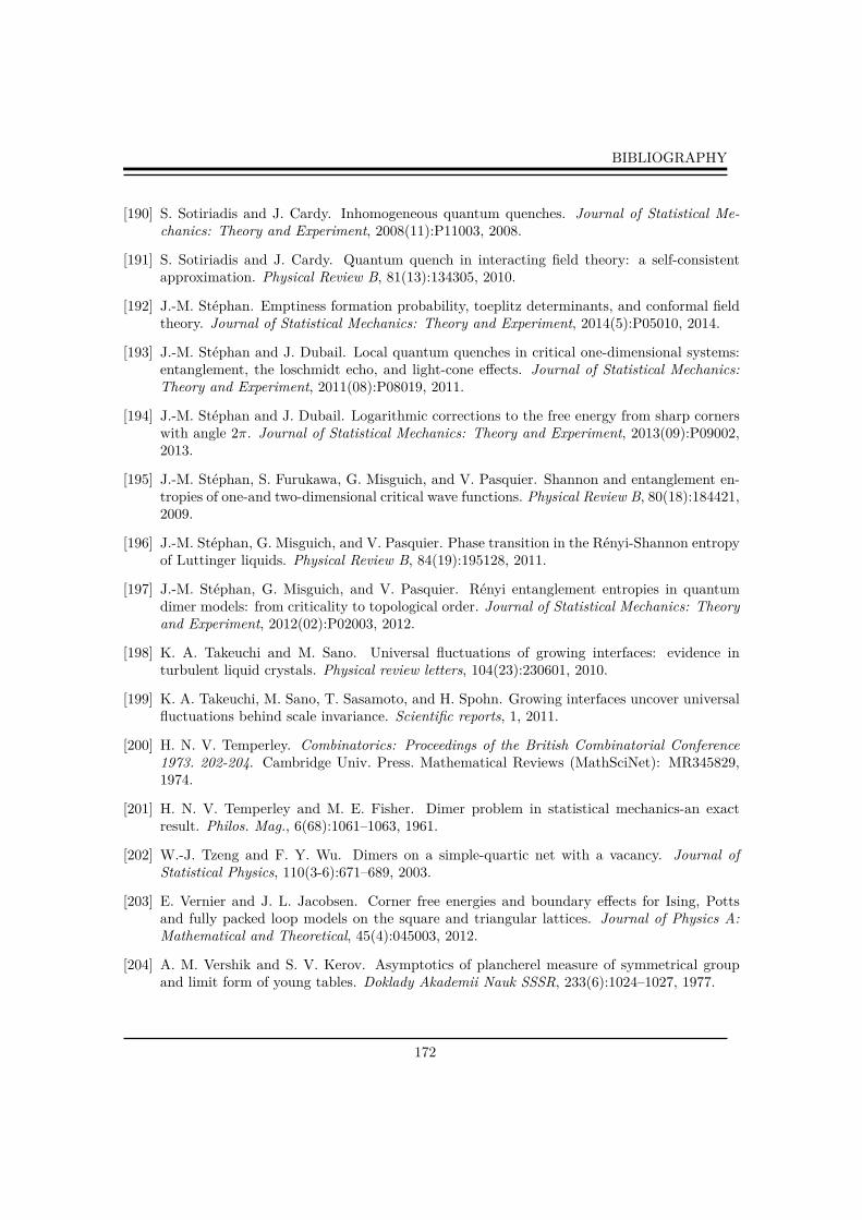
BIBLIOGRAPHY
[190] S. Sotiriadis and J. Cardy. Inhomogeneous quantum quenches. Journal of Statistical Me-chanics: Theory and Experiment, 2008(11):P11003, 2008.
[191] S. Sotiriadis and J. Cardy. Quantum quench in interacting field theory: a self-consistentapproximation. Physical Review B, 81(13):134305, 2010.
[192] J.-M. Stéphan. Emptiness formation probability, toeplitz determinants, and conformal fieldtheory. Journal of Statistical Mechanics: Theory and Experiment, 2014(5):P05010, 2014.
[193] J.-M. Stéphan and J. Dubail. Local quantum quenches in critical one-dimensional systems:entanglement, the loschmidt echo, and light-cone effects. Journal of Statistical Mechanics:Theory and Experiment, 2011(08):P08019, 2011.
[194] J.-M. Stéphan and J. Dubail. Logarithmic corrections to the free energy from sharp cornerswith angle 2π. Journal of Statistical Mechanics: Theory and Experiment, 2013(09):P09002,2013.
[195] J.-M. Stéphan, S. Furukawa, G. Misguich, and V. Pasquier. Shannon and entanglement en-tropies of one-and two-dimensional critical wave functions. Physical Review B, 80(18):184421,2009.
[196] J.-M. Stéphan, G. Misguich, and V. Pasquier. Phase transition in the Rényi-Shannon entropyof Luttinger liquids. Physical Review B, 84(19):195128, 2011.
[197] J.-M. Stéphan, G. Misguich, and V. Pasquier. Rényi entanglement entropies in quantumdimer models: from criticality to topological order. Journal of Statistical Mechanics: Theoryand Experiment, 2012(02):P02003, 2012.
[198] K. A. Takeuchi and M. Sano. Universal fluctuations of growing interfaces: evidence inturbulent liquid crystals. Physical review letters, 104(23):230601, 2010.
[199] K. A. Takeuchi, M. Sano, T. Sasamoto, and H. Spohn. Growing interfaces uncover universalfluctuations behind scale invariance. Scientific reports, 1, 2011.
[200] H. N. V. Temperley. Combinatorics: Proceedings of the British Combinatorial Conference1973. 202-204. Cambridge Univ. Press. Mathematical Reviews (MathSciNet): MR345829,1974.
[201] H. N. V. Temperley and M. E. Fisher. Dimer problem in statistical mechanics-an exactresult. Philos. Mag., 6(68):1061–1063, 1961.
[202] W.-J. Tzeng and F. Y. Wu. Dimers on a simple-quartic net with a vacancy. Journal ofStatistical Physics, 110(3-6):671–689, 2003.
[203] E. Vernier and J. L. Jacobsen. Corner free energies and boundary effects for Ising, Pottsand fully packed loop models on the square and triangular lattices. Journal of Physics A:Mathematical and Theoretical, 45(4):045003, 2012.
[204] A. M. Vershik and S. V. Kerov. Asymptotics of plancherel measure of symmetrical groupand limit form of young tables. Doklady Akademii Nauk SSSR, 233(6):1024–1027, 1977.
172

BIBLIOGRAPHY
[205] D. Vukičević. Applications of perfect matchings in chemistry. In Structural Analysis ofComplex Networks, page 463. Springer, 2010.
[206] D. Vukičević. Applications of perfect matchings in chemistry. In Structural Analysis ofComplex Networks, pages 463–482. Springer, 2011.
[207] D. Vvedensky, A. Zangwill, C. Luse, and M. Wilby. Stochastic equations of motion forepitaxial growth. Physical Review E, 48(2):852, 1993.
[208] F. Wang and F. Y. Wu. Exact solution of close-packed dimers on the Kagomé lattice. PhysicalReview E, 75(4):040105, 2007.
[209] F. Wang and F. Y. Wu. Dimers on the Kagomé lattice II: Correlations and the Grassmannianapproach. Physica A: Statistical Mechanics and its Applications, 387(16):4157–4162, 2008.
[210] D. E. Wolf and L.-H. Tang. Inhomogeneous growth processes. Physical review letters,65(13):1591, 1990.
[211] F. W. Wu. Ising model with four-spin interactions. Physical Review B, 4(7):2312–2314, 1971.
[212] F. Y. Wu. Dimers on two-dimensional lattices. International Journal of Modern Physics B,20(32):5357–5371, 2006.
[213] F. Y. Wu, W.-J. Tzeng, and N. S. Izmailian. Exact solution of a monomer-dimer problem: Asingle boundary monomer on a nonbipartite lattice. Physical Review E, 83(1):011106, 2011.
[214] F. Y. Wu and F. Wang. Dimers on the kagome lattice I: Finite lattices. Physica A: StatisticalMechanics and its Applications, 387(16):4148–4156, 2008.
[215] W. Yan, Y.-N. Yeh, and F. Zhang. Dimer problem on the cylinder and torus. Physica A:Statistical Mechanics and its Applications, 387(24):6069–6078, 2008.
[216] Z. Zhang, Y. Sheng, and Q. Jiang. Monomer–dimer model on a scale-free small-world net-work. Physica A: Statistical Mechanics and its Applications, 391(3):828–833, 2012.
[217] W. Zheng and S. Sachdev. Sine-Gordon theory of the non-Néel phase of two-dimensionalquantum antiferromagnets. Physical Review B, 40(4):2704, 1989.
[218] P. Zinn-Justin. Six-vertex model with domain wall boundary conditions and one-matrixmodel. Physical Review E, 62(3):3411, 2000.
173

Critical Properties of Dimers, Spin Chains and Interface Models
The study carried in this thesis concerns classical and quantum critical phenomena. Indeed, critical be-haviors and phase transitions are fundamental topics in modern statistical physics and field theory and wepropose in this thesis to study some models which exhibit such behaviors both at equilibrium and out ofequilibrium. In the first part of the thesis, some properties of the two-dimensional dimer model are studied.This model has been studied extensively in the statistical physics and mathematical communities and a lot ofapplications in condensed matter physics exist. Here we propose to focus on exact solutions of the model andconformal invariance in order to have a deep understanding of this model in presence of monomers, and/orboundaries. The same kind of tools are then used to explore another important phenomenon appearing indimer models and spin chains: the arctic circle. The goal was to find a proper field theoretical descriptionof this phenomenon using exact solutions and asymptotic analysis. The second part of the thesis concernsout of equilibrium critical phenomena in the context of interface growth models. This field of research isvery important nowadays, mainly because of the Kardar-Parisi-Zhang equation and its relations with ran-dom matrix ensembles. The phenomenology of these models in presence of boundaries is studied via exactsolutions and numerical simulations, we show that surprising behaviors appear close to the boundaries.
Key-words: Critical phenomena, dimer models, Grassmann algebra, conformal invariance, spin chains, outof equilibrium statistical physics, interface growth, KPZ equation.
Propriétés critiques des modèles de dimères, de chaînes de spin et d’interfaces
L’étude réalisée dans cette thèse porte sur les phénomènes critiques classiques et quantiques. En effet,les phénomènes critiques et les transitions de phases sont devenues des sujets fondamentaux en physiquestatistique moderne et en théorie des champs et nous proposons dans cette thèse d’étudier certains modèlesqui présentent un comportement critique à la fois à l’équilibre et hors de l’équilibre. Dans la première partiede la thèse, certaines propriétés du modèle de dimères à deux dimensions sont étudiées. Ce modèle a étélargement étudié dans les communautés de physique statistique et de mathématiques et un grand nombred’applications en physique de la matière condensée existent. Ici, nous proposons de mettre l’accent sur dessolutions exactes du modèle et d’utiliser l’invariance conforme afin d’avoir une compréhension profonde dece modèle en présence de monomères et/ou en présence de bords. Les mêmes types d’outils sont ensuiteutilisés pour explorer un autre phénomène important apparaissant dans les modèles de dimères et de chaînesde spin: le cercle arctique. Le but étant de trouver une description adéquate en terme de théorie des champsde ce phénomène en utilisant des calculs exacts ainsi que de l’analyse asymptotique. La deuxième partiede la thèse concerne les phénomènes critiques hors de l’équilibre dans le contexte des modèles de croissanced’interfaces. Ce domaine de recherche est très important de nos jours, principalement en raison de ladécouverte de l’équation Kardar-Parisi-Zhang et de ses relations avec les ensembles de matrices aléatoires. Laphénoménologie de ces modèles en présence des bords est analysé via des solutions exactes et des simulationsnumériques, on montre alors que des comportements surprenants apparaissent proche des bords.
Mots-clés: Phénomènes critiques, modèles de dimères, algèbre de Grassmann, invariance conforme, physiquestatistique hors-équilibre, croissance d’interface, équation de KPZ.