Lifelong Reinforcement Learning with Temporal Logic Formulasand Reward Machines

Xuejing Zheng1, Chao Yu1*, Chen Chen2, Jianye Hao2, Hankz Hankui Zhuo1

1 Dept. of Computer Science, Sun Yat-sen University2 Huawei Noah’s Ark Lab

zhengxj28@mail2.sysu.edu.cn, yuchao3@mail.sysu.edu.cn, chenchen9@huawei.com, haojianye@huawei.com,zhuohank@mail.sysu.edu.cn

Abstract

Continuously learning new tasks using high-level ideas orknowledge is a key capability of humans. In this paper, wepropose Lifelong reinforcement learning with Sequential lin-ear temporal logic formulas and Reward Machines (LSRM),which enables an agent to leverage previously learned knowl-edge to fasten learning of logically specified tasks. For thesake of more flexible specification of tasks, we first introduceSequential Linear Temporal Logic (SLTL), which is a sup-plement to the existing Linear Temporal Logic (LTL) formallanguage. We then utilize Reward Machines (RM) to exploitstructural reward functions for tasks encoded with high-levelevents, and propose automatic extension of RM and efficientknowledge transfer over tasks for continuous learning in life-time. Experimental results show that LSRM outperforms themethods that learn the target tasks from scratch by taking ad-vantage of the task decomposition using SLTL and knowl-edge transfer over RM during the lifelong learning process.

1 IntroductionThere are at least two significant abilities of human intelli-gence: (i) storing learned skills in memory over lifetime andleveraging them when encountering new tasks; and (ii) uti-lizing high-level ideas or knowledge for more efficient rea-soning and learning. These abilities enable humans to adaptquickly in environments where tasks and experiences changeover time. Lifelong Reinforcement Learning (LRL) (Abelet al. 2018; Brunskill and Li 2014; Garcia and Thomas 2019)formalizes the problem of building taskable agents by ex-ploiting knowledge gained in previous tasks to improve per-formance in new but related tasks. Solving the LRL problemis an essential step toward general artificial intelligence as itallows agents to continuously adapt to changes in the envi-ronment with minimal human intervention, which is a keyfeature of human learning.

There has recently been a surge of interest in methodsfor achieving efficient LRL, utilizing techniques such as net-work consolidation (Schwarz et al. 2018) or freezing (Rusuet al. 2016), rehearsal via experience replay (Isele and Cos-gun 2018; Rolnick et al. 2018), and value-function/policyinitialization (Abel et al. 2018). Remarkably, the line ofthese works has mainly focused on the continuous learning

Copyright © 2022, Association for the Advancement of ArtificialIntelligence (www.aaai.org). All rights reserved.

settings, where a series of related tasks are drawn from a taskdistribution. Attention is restricted to subclasses of MDPsby making structural assumptions about which MDP com-ponents (rewards or transition probabilities) may change insupport of the generation of tasks. While this kind of as-sumptions is reasonable in most real life situations, thereare also scenarios when either task specification is non-Markovian and thus difficult to be expressed analytically asa reward function, or the sequential tasks cannot be gener-ated from an underlying distribution when expressed logi-cally using formal languages (Linz 2006; Pnueli 1977). Forinstance, consider a scenario when an agent has learned thetask of “delivering coffee and mail to office”. When facing anew task of “delivering coffee or mail to office”, it is unclearhow existing LRL methods would model these tasks as thesame distribution of MDP and enable efficient transfer learn-ing among these tasks. This limitation contradicts the humanability of compositional learning using high-level ideas orknowledge, i.e., understanding novel situations by combin-ing and reasoning over already known primitives.

In this paper, we investigate LRL problems when the se-ries of tasks do not necessarily share the same MDP struc-ture, but instead are specified with high-level events usingLinear Temporal Logic (LTL) (Li, Vasile, and Belta 2017;Toro Icarte et al. 2018). The basic intuition is to exploit taskmodularity and decomposition with higher abstraction andsuccinctness to facilitate transfer learning in target tasks.We first introduce the Sequential Linear Temporal Logic(SLTL), which is a supplement to LTL by adding a new op-erator “then”, and also prove the operator laws of SLTL toprovide more flexible and rich specification of a task. In or-der to enable more efficient task learning, Reward Machines(RM) (Icarte et al. 2018) are utilized to express structuralreward functions for tasks encoded with high-level events.Synthesizing the merits of task modularity using SLTL andpolicy learning over RM, we propose the Lifelong reinforce-ment learning with SLTL and RM (LSRM) method, whichstores and leverages high-level knowledge in a memory formore efficient lifelong learning of logically specified tasks.The memory contains an RM, which can be automaticallyupdated when facing a set of target tasks, and the high-levelknowledge stored in the memory can be transferred to anew decomposed target task using a number of value com-position methods. We evaluate the performance of LSRM

arX

iv:2

111.

0947

5v1

[cs

.AI]

18

Nov

202

1

in the OFFICEWORLD and MINECRAFT domains. Exper-iments show that LSRM enables the agent to learn targettasks more efficiently compared to the direct methods with-out transfer learning.

The remaining part of the paper is organized as follows.Section 2 provides a background introduction. Section 3 in-troduces the SLTL language. Section 4 presents the LSRMand Section 5 provides experimental studies. Section 6 re-views some related works, and finally, Section 7 concludeswith some directions of future work.

2 PreliminariesWe provide a preliminary introduction to RL, LTL and RMin this section. Please refer to (Sutton and Barto 2018; Pnueli1977; Toro Icarte et al. 2020) for more details in these topics.

2.1 RLThe RL problem consists of an agent interacting with an un-known environment (Sutton and Barto 2018), which can bemodeled as a Markov Decision Process (MDP) by a tupleM = (S,A, r, p, γ), where S is a finite set of states, A is afinite set of actions, r : S×A×S → R is a reward function,p : S ×A×S → [0, 1] is a probabilistic transition function,and γ ∈ (0, 1] is a discount factor.

A policy is a mapping π : S × A → [0, 1], and π(s, a)means the probability of choosing action a in state s. TheQ-function Qπ(s, a) following the policy π is the expecteddiscounted reward of choosing action a in state s under pol-icy π, i.e., Qπ(s, a) = Eπ[

∑∞k=0 γ

krt+k+1 | st = s, at =a], where sk+1 ∼ p(sk, ak, ·), rk+1 = r(sk, ak, sk+1), andak ∼ π(sk, ·). The goal of RL is to learn an optimal pol-icy π∗, which maximizes the expected discounted rewardfor each s ∈ S, a ∈ A, i.e., Q∗(s, a) := Qπ∗(s, a) =maxπ Qπ(s, a). A well-known approach for calculating theoptimal Q-function in tabular case is Q-learning (Watkinsand Dayan 1992). Its one-step updating rule is given byQ(s, a)

α←− r(s, a, s′) + γmaxa′ Q(s′, a′), where x α←− ymeans x ← x + α(y − x). The action a is chosen by us-ing certain exploration strategies, such as the ε-greedy pol-icy, i.e., choosing a random action with probability ε, whilechoosing argmaxa′ Q(s, a′) with probability 1− ε.

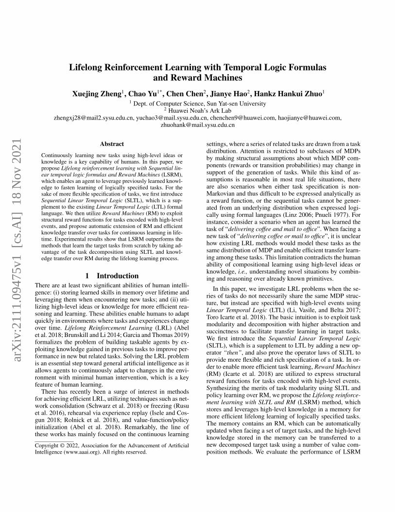
2.2 LTLLTL is a propositional modal logic with temporal modalities(Pnueli 1977). It has been used to specify tasks encoded withhigh-level events in RL by characterizing the successful andunsuccessful executions (Toro Icarte et al. 2018; Li, Vasile,and Belta 2017). Each high-level event is represented by apropositional variable, and the set of all propositional vari-ables is denoted by P . The set of events that occur at timet = i under state si is a label, denoted by li ⊆ P , which isgiven by a labelling function L : S → 2P , li = L(si). As anillustrative example, consider the OFFICEWORLD domainpresented in Figure 1(a). The propositional variables can beP = {c,m, o, ∗, A,B,C,D}, where c is “getting coffee”,m is “getting mail”, o is “at office”, ∗ is “furniture”, andA,B,C,D is “at A, B, C, D”, respectively. An event p ∈ Poccurs if and only if the agent is located at the grid marked

by p. Hence the labelling function is L(s) = {p} if s ismarked by p, and L(s) = ∅ otherwise. Given the proposi-tional variables P , LTL formulas can be conducted from thestandard Boolean operators ∧ (and), ¬ (negation), and tem-poral operators © (next), U (until). Other operators can bederived from the operators above. For example, the operator∨ (or) and ♦ (eventually) are defined as ϕ∨ψ = ¬(¬ϕ∧¬ψ)and ♦ϕ = >Uϕ, respectively, where > = ϕ ∨ ¬ϕ is theformula “true”. Formally, the syntax of an LTL formula isdefined as ϕ := p | ¬ϕ | ϕ ∧ ψ | ©ϕ | ϕUψ, where p ∈ P .

The semantic of LTL is defined over an infinite sequenceof labels, denoted λ = l0l1l2 · · · . We use λ |= ϕ to denotethat an LTL formula ϕ is determined to be true by a sequenceλ, which is formally defined as follows: (i) λ |= p⇔ p ∈ l0,where p ∈ P; (ii) λ |= ¬ϕ⇔ λ 6|= ϕ; (iii) λ |= ϕ1 ∧ ϕ2 ⇔λ |= ϕ1 and λ |= ϕ2; (iv) λ |= ©ϕ ⇔ λ1 |= ϕ; and (v)λ |= ϕ1Uϕ2 ⇔ ∃j > 0, λj |= ϕ2 and ∀i ≤ j, λi |= ϕ1.The notation λi denotes the postfix lili+1li+2 · · · of thesequence. Based on the above definitions, we can definetasks using LTL formulas. For instance, the task “eventuallyreaching office” is defined as ♦o, and the task “deliveringcoffee to office” is defined as ♦(c ∧©♦o).

In order to specify the remaining module of a task afterproceeding a sequence of labels, LTL progression (Bacchusand Kabanza 2000) has been proposed. For example, we canprogress the formula ♦(c ∧ ©♦o) by a label {c} and get anew formula ♦o, implying that the remaining task is “go-ing to office” after getting the coffee. Formally, an LTL pro-gression maps an LTL formula ϕ and a label l to anotherLTL formula, denoted as prog(ϕ, l), which is defined recur-sively as follows: (i) prog(p, l) = > if p ∈ l, where p ∈ P;(ii) prog(¬ϕ, l) = ¬prog(ϕ, l); (iii) prog(ϕ1 ∧ ϕ2, l) =prog(ϕ1, l) ∧ prog(ϕ2, l); (iv) prog(©ϕ, l) = ϕ; and (v)prog(ϕ1Uϕ2, l) = prog(ϕ2, l) ∨ (prog(ϕ1, l) ∧ ϕ1Uϕ2). Ithas been theoretically proved that a sequence of labels satis-fies an LTL formula if and only if the postfix of the sequencesatisfies the progressed formulas, i.e., λi |= ϕ ⇔ λi+1 |=prog(ϕ, li) (Bacchus and Kabanza 2000).

2.3 RMRM can be used to reveal the structure of non-Markovianreward functions of tasks that are encoded with high-levelevents (i.e., propositional variables), formally defined as fol-lows (Toro Icarte et al. 2020).

Definition 1. Given the propositional variables P and aset of all possible labels Σ ⊆ 2P , an RM is a tuple R =(U, u0, F, δ, R), where U is a finite set of states, u0 is an ini-tial state, F ⊆ U are terminal states, δ : U × Σ → U isthe transition function, and R : U × Σ → R is the rewardfunction.

Distinguished from the states of the environment (denotedby s), the states of RM (denoted by u) and the transitionsamong them are generally given by the prior knowledge ofspecific tasks. Figure 1(b) gives an example of RM that rep-resents the task “eventually getting coffee and mail” in OF-FICEWORLD, where the nodes are states and the edges aretransitions among states. Each transition is encoded with atuple (l1, l2, · · · , ln | r), where each li is a label and r is the

(a) OFFICEWORLD. (b) An example of RM.

(c) Encoding RM with LTL. (d) Reward shaping for RM.

Figure 1: Illustrations of the OFFICEWORLD environmentand RM.

output reward. The initial state is colored in yellow and theterminal state is colored in red. In order to enrich the expres-siveness of RM, each state of RM can also be encoded withan LTL formula (Figure 1(c)), implying a portion of a taskthat the agent has not completed yet. Especially, the terminalstates are encoded with >(true) or ⊥(false), which indicatesthe completion or failure of a task, respectively. When anRM transits to terminal states, the current episode ends. Thereward function of RM is then defined as follows:

R(ψ, l) =

{1, if ψ 6= >, δ(ψ, l) = >;

0, otherwise.(1)

In order to induce denser rewards than binary rewards above,automatic reward shaping for RM (Camacho et al. 2019;Toro Icarte et al. 2020) is proposed. It modifies the rewardfunction asR′(ψ, l) = R(ψ, l)+γΦ(δ(ψ, l))−Φ(ψ), whereΦ : U → R is the potential function calculated by value it-eration. The modified reward function of the example aboveis presented in Figure 1(d).

The QRM algorithm (Icarte et al. 2018) is then proposedto leverage RM to learn tasks. QRM maintains a Q-functionQu for each RM state u ∈ U (or formula), and updatesall the Q-functions using internal rewards and transitions ofRM with one experience (s, a, s′). Formally, the Q-functionof each state in RM is updated by

Qu(s, a)α←− R(u, l) + γmax

a′Qu′(s′, a′),∀u ∈ U (2)

where l = L(s) is the current label,R(u, l) is the internal re-ward and u′ = δ(u, l) is the internal next state of RM. QRMnot only converges to an optimal policy in tabular cases, butalso outperforms the Hierarchical RL (HRL) methods whichmight converge to suboptimal policies (Icarte et al. 2018).

3 SLTL: Sequential Linear Temporal LogicIn order to enable decomposition of sequential tasks, we adda new temporal operator∼(then) into the traditional LTL, re-sulting the Sequential LTL (SLTL). Being compatible withLTL, SLTL provides a more succinct and flexible way todescribe sequential tasks, and more importantly, enables usto exploit task modularity for more efficient transfer learn-ing than LTL. For example, the task “eventually complete athen b” is expressed as ♦(a ∧©(♦b)) using LTL, but moredirectly as (♦a) ∼ (♦b) using SLTL. The latter expressioncan be decomposed into subtasks ♦a and ♦b, the knowledgeof which can be readily transferred to the learning of targettask, say (♦b) ∼ (♦a). However, such straightforward ma-nipulation cannnot be readily realized using the expressionof LTL, since we cannot extract ♦a from the LTL formula of♦(a∧©(♦b)). Please refer to Appendix.A. for more detailsin the syntax and semantics of SLTL.

We prove the laws of the operator “then” to provide dif-ferent ways of decomposing a target task.Theorem 1. For any SLTL formulas ϕ1, ϕ2, ϕ3, we have theassociative law: (ϕ1 ∼ ϕ2) ∼ ϕ3 = ϕ1 ∼ (ϕ2 ∼ ϕ3), andthe following distribution laws:

(i) (ϕ1 ∼ ϕ2) ∧ (ϕ1 ∼ ϕ3) = ϕ1 ∼ (ϕ2 ∧ ϕ3);(ii) (ϕ1 ∼ ϕ3) ∧ (ϕ2 ∼ ϕ3) = (ϕ1 ∧ ϕ2) ∼ ϕ3;

(iii) (ϕ1 ∼ ϕ2) ∨ (ϕ1 ∼ ϕ3) = ϕ1 ∼ (ϕ2 ∨ ϕ3);(iv) (ϕ1 ∼ ϕ3) ∨ (ϕ2 ∼ ϕ3) = (ϕ1 ∨ ϕ2) ∼ ϕ3.

Proof. See Appendix.A.

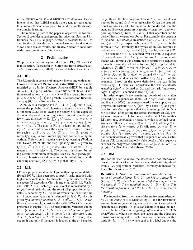
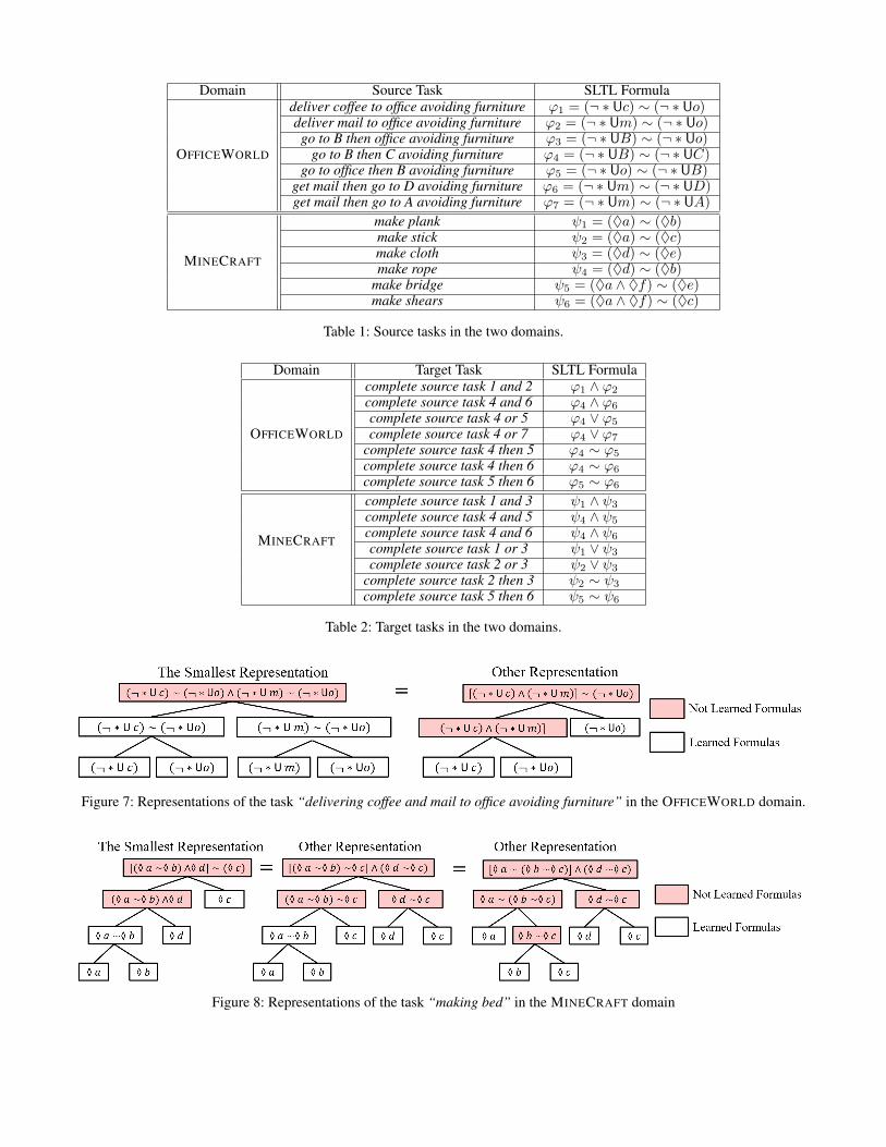
Figure 2: Two different ways of task decomposition usingthe operator laws.

The above operator laws enable various representationsof a task, leading to different ways of task decompositionand thus diverse learning efficiency. Figure 2 gives an il-lustration: the two formulas on the top are equivalent rep-resentations of the same target task. Suppose that formulasa ∼ b, c, d (colored in white) indicate the subtasks that havebeen learned before (i.e., learned formulas), while the re-maining formulas (colored in red) indicate the new tasks thathave not been learned yet. It is clear that the left presenta-tion has fewer new subtasks than the right one. More for-mally, we define the smallest representation of a task usingthe operator laws as follows:Definition 2. Let ϕ1, ϕ2, · · · , ϕn be the different represen-tations of a target task, and T1, T2, · · · , Tn be their sub-formulas decomposed by the ∧,∨,∼ operators. Given a setof learned formulas TM , the smallest representation ϕ∗ ofthe target task is the one with the smallest number of sub-tasks that have been not learned before, i.e.,

ϕ∗ = ϕi, where i = argmini=1,2,··· ,n

|Ti \ TM |. (3)

The consideration of the smallest representation of a tar-get task can be attributed to the fact that when facing a newtask, it is more likely to learn faster if the task can be decom-posed into fewer unknown subtasks. We will provide exper-imental evaluations on this issue in Subsec. 5.2.

4 LSRM: Lifelong Learning with SLTLand RM

In this section, we introduce the LSRM method that com-bines the benefits of both SLTL and RM for efficient learn-ing of logically specified tasks. Formally, LSRM maintainsa memoryM = (RM , TM ,QM ) for the agent over lifetime,where RM = (UM , u0, F, δ, R) is the memory RM, TM isthe set of learned SLTL formulas from previous tasks, andQM = {Qϕ(s, a) | ϕ ∈ UM} is the set of Q-functions cor-responding to the states in RM . In a learning phase of thelifetime, the agent is required to learn a set of target tasks,and different representations of these tasks can be generatedby the operator laws. The smallest representation of the tar-get task is then chosen according to the learned formulas TMin the memory, and then fed into Algorithm 1 as a set of tar-get formula(s) T . Concretely, for each target formula ϕ inT , LSRM first extends the memory RM and returns its newextended states denoted as Uϕnew (Line 2-3). The learned Q-functions are then transferred from the memory to the newQ-function corresponding to each state in Uϕnew (Line 4-5).Finally, the QRM algorithm is utilized to learn the target for-mulas (Line 8). When the agent starts to implement a taskϕ ∈ T in an episode of QRM, the initial state of the mem-ory RM is set to be u0 = ϕ. The set of learned task TMis then updated after the QRM learning procedure (Line 9).We show the details of extension of the memory RM andtransferring knowledge in the following subsections.

Algorithm 1: The Update of the Memory in LSRMInput: Set of target formula(s) T , memory MOutput: New memory M

1: for all target formula ϕ ∈ T do2: M .ExtendRM(ϕ)3: Uϕnew ←M .ReturnNewStates()4: for all extended state ψ ∈ Uϕnew do5: Qψ(s, a)←M .AcquireKnowledge(ψ)6: end for7: end for8: M .QRMRun(T )9: TM ← (∪ϕ∈TUϕnew) ∪ TM

4.1 Extensions of Memory RMIn this subsection, we discuss how to extend the memoryRM with a target task prescribed by an SLTL formula, sothat the extended RM includes all the modules of the targettask for future learning. On one hand, the target formula canbe iteratively progressed in order to extract sub-formulas us-ing the SLTL progression, inspired by LTL Progression forOff-Policy Learning (Toro Icarte et al. 2018). On the otherhand, it can also be decomposed using the “then” operator

to extract sub-formulas accounting for the possibly encoun-tered tasks in the future. Each extracted sub-formula by ei-ther progression or decomposition indicates a module of thetarget task. Whenever an extracted formula is new, i.e., not inthe states UM of the original memory RM, the formula andits corresponding transitions will be stored as an extendedstate of the RM.

Formally, for each input target formula ϕ, the set of ex-tracted formulas is initialized as Tex = {ϕ} and iterativelyupdated by:

Tex ← Tex ∪ Tprog ∪ Tdec, (4)where Tprog = {prog(ψ, l) | ψ ∈ Tex, l ∈ Σ} is the setof formulas progressed by all the labels, and Tdec = {ψ1 |ψ ∈ Tex, ψ = ψ1 ∼ ψ2} is the set of sub-formulas decom-posed by the∼ operator. The iteration terminates if and onlyif the set Tex does not change anymore. Denote the origi-nal memory RM as RM = (UM , u0, F, δ, R), then the newstates are Unew = Tex \ UM . Therefore, the extended RMis R′M = (U ′M , u0, F

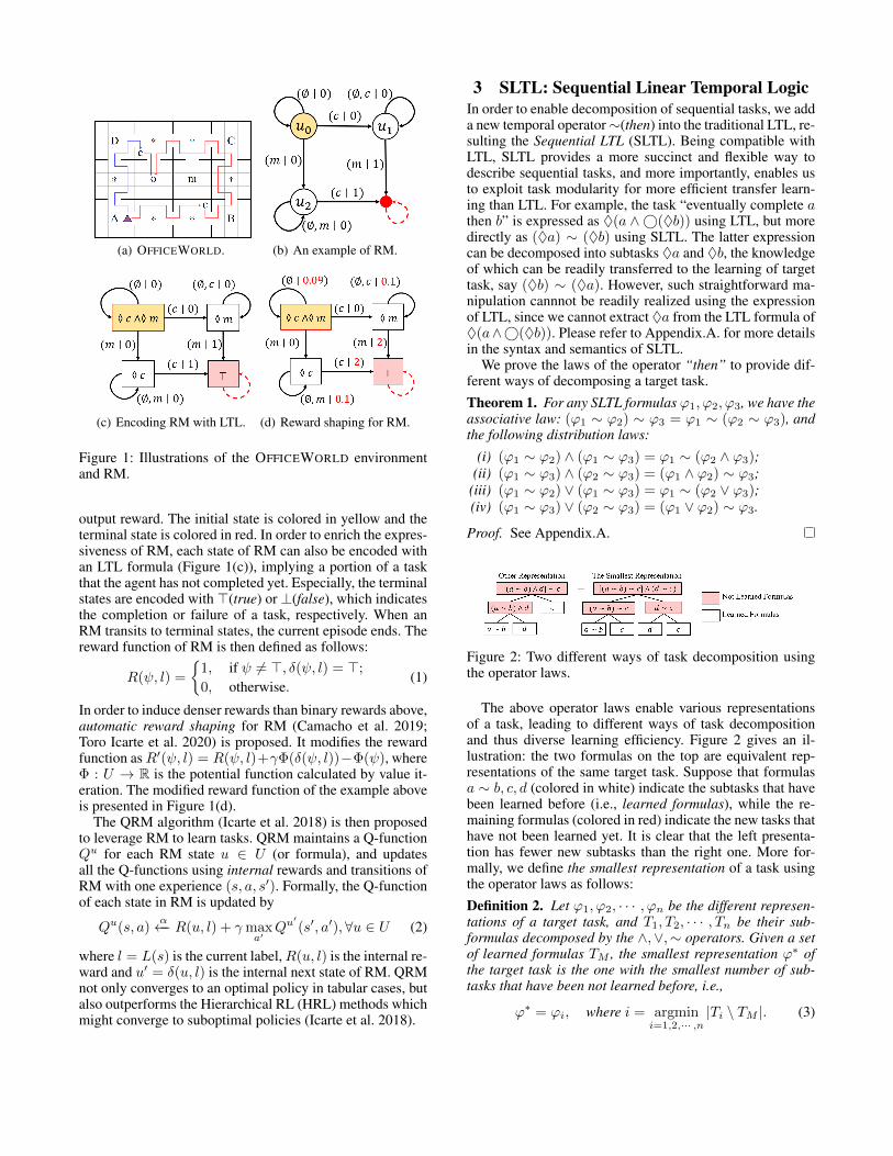
′, δ′, R′), where the states are U ′M =UM ∪ Unew; the transition function is δ′(ψ, l) = δ(ψ, l) fororiginal states ψ ∈ UM and δ′(ψ, l) = prog(ψ, l) for newstates ψ ∈ Unew; the terminal states are F ′ = U ′M ∩{>,⊥};and the reward functionR′ is defined as Eq. (1). Algorithm 2gives the procedure of extending RM and Figure 3 plots anillustrative example of such a process.

Algorithm 2: ExtendRM(ϕ)Input: Memory M , the target SLTL formula ϕOutput: New memory M

1: if ϕ ∈ UM then2: return3: else4: Initialize queue=[ϕ], UM ← UM ∪ {ϕ}5: while not queue.empty() do6: ψ ← queue.pop()7: if ψ = ψ1 ∼ ψ2 and ψ1 6∈ UM then8: UM ← UM ∪ {ψ1}, queue.append(ψ1)9: end if

10: for all l ∈ Σ do11: ψ′ = prog(ψ, l)12: if ψ′ 6∈ UM then13: UM ← UM ∪ {ψ′}, queue.append(ψ′)14: end if15: Store transition δ(ψ, l) = ψ′ forRM16: end for17: end while18: end if

4.2 Acquisition of Knowledge from the MemoryThe key idea to acquire knowledge, i.e., Q-functions fromthe memory for a target formula ϕ, is to iteratively decom-pose the target formula ϕ into sub-formulas until all thesub-formulas are in the learned tasks TM , such that the Q-function of the target formula ϕ can be initialized using thecomposed Q-values of the learned sub-formulas. If the in-put formula ψ has been learned, then its corresponding Q-function is returned directly. If ψ has not been learned but

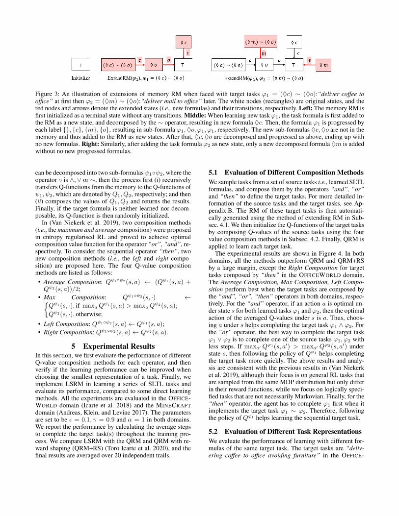
Figure 3: An illustration of extensions of memory RM when faced with target tasks ϕ1 = (♦c) ∼ (♦o):“deliver coffee tooffice” at first then ϕ2 = (♦m) ∼ (♦o):“deliver mail to office” later. The white nodes (rectangles) are original states, and thered nodes and arrows denote the extended states (i.e., new formulas) and their transitions, respectively. Left: The memory RM isfirst initialized as a terminal state without any transitions. Middle: When learning new task ϕ1, the task formula is first added tothe RM as a new state, and decomposed by the ∼ operator, resulting in new formula ♦c. Then, the formula ϕ1 is progressed byeach label {}, {c}, {m}, {o}, resulting in sub-formula ϕ1,♦o, ϕ1, ϕ1, respectively. The new sub-formulas ♦c,♦o are not in thememory and thus added to the RM as new states. After that, ♦c,♦o are decomposed and progressed as above, ending up withno new formulas. Right: Similarly, after adding the task formula ϕ2 as new state, only a new decomposed formula ♦m is addedwithout no new progressed formulas.

can be decomposed into two sub-formulas ψ1◦ψ2, where theoperator ◦ is ∧,∨ or ∼, then the process first (i) recursivelytransfers Q-functions from the memory to the Q-functions ofψ1, ψ2, which are denoted byQ1, Q2, respectively; and then(ii) composes the values of Q1, Q2 and returns the results.Finally, if the target formula is neither learned nor decom-posable, its Q-function is then randomly initialized.

In (Van Niekerk et al. 2019), two composition methods(i.e., the maximum and average composition) were proposedin entropy regularised RL and proved to achieve optimalcomposition value function for the operator “or”, “and”, re-spectively. To consider the sequential operator “then”, twonew composition methods (i.e., the left and right compo-sition) are proposed here. The four Q-value compositionmethods are listed as follows:• Average Composition: Qψ1◦ψ2(s, a) ← (Qψ1(s, a) +Qψ2(s, a))/2;

• Max Composition: Qψ1◦ψ2(s, ·) ←{Qψ1(s, ·), if maxaQ

ψ1(s, a) > maxaQψ2(s, a);

Qψ2(s, ·), otherwise;

• Left Composition: Qψ1◦ψ2(s, a)← Qψ1(s, a);• Right Composition: Qψ1◦ψ2(s, a)← Qψ2(s, a).

5 Experimental ResultsIn this section, we first evaluate the performance of differentQ-value composition methods for each operator, and thenverify if the learning performance can be improved whenchoosing the smallest representation of a task. Finally, weimplement LSRM in learning a series of SLTL tasks andevaluate its performance, compared to some direct learningmethods. All the experiments are evaluated in the OFFICE-WORLD domain (Icarte et al. 2018) and the MINECRAFTdomain (Andreas, Klein, and Levine 2017). The parametersare set to be ε = 0.1, γ = 0.9 and α = 1 in both domains.We report the performance by calculating the average stepsto complete the target task(s) throughout the training pro-cess. We compare LSRM with the QRM and QRM with re-ward shaping (QRM+RS) (Toro Icarte et al. 2020), and thefinal results are averaged over 20 independent trails.

5.1 Evaluation of Different Composition MethodsWe sample tasks from a set of source tasks i.e., learned SLTLformulas, and compose them by the operators “and”, “or”and “then” to define the target tasks. For more detailed in-formation of the source tasks and the target tasks, see Ap-pendix.B. The RM of these target tasks is then automati-cally generated using the method of extending RM in Sub-sec. 4.1. We then initialize the Q-functions of the target tasksby composing Q-values of the source tasks using the fourvalue composition methods in Subsec. 4.2. Finally, QRM isapplied to learn each target task.

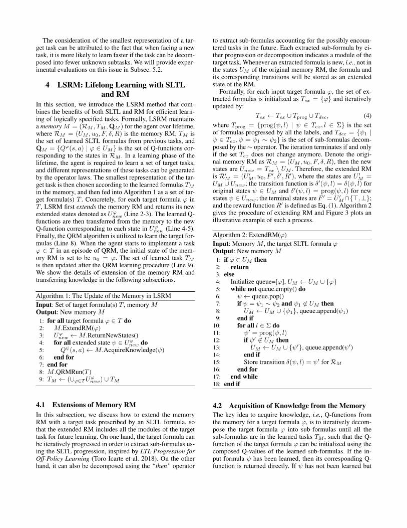
The experimental results are shown in Figure 4. In bothdomains, all the methods outperform QRM and QRM+RSby a large margin, except the Right Composition for targettasks composed by “then” in the OFFICEWORLD domain.The Average Composition, Max Composition, Left Compo-sition perform best when the target tasks are composed bythe “and”, “or”, “then” operators in both domains, respec-tively. For the “and” operator, if an action a is optimal un-der state s for both learned tasks ϕ1 and ϕ2, then the optimalaction of the averaged Q-values under s is a. Thus, choos-ing a under s helps completing the target task ϕ1 ∧ ϕ2. Forthe “or” operator, the best way to complete the target taskϕ1 ∨ ϕ2 is to complete one of the source tasks ϕ1, ϕ2 withless steps. If maxa′ Q

ϕ1(s, a′) > maxa′ Qϕ2(s, a′) under

state s, then following the policy of Qϕ1 helps completingthe target task more quickly. The above results and analy-sis are consistent with the previous results in (Van Niekerket al. 2019), although their focus is on general RL tasks thatare sampled from the same MDP distribution but only differin their reward functions, while we focus on logically speci-fied tasks that are not necessarily Markovian. Finally, for the“then” operator, the agent has to complete ϕ1 first when itimplements the target task ϕ1 ∼ ϕ2. Therefore, followingthe policy of Qϕ1 helps learning the sequential target task.

5.2 Evaluation of Different Task RepresentationsWe evaluate the performance of learning with different for-mulas of the same target task. The target tasks are “deliv-ering coffee to office avoiding furniture” in the OFFICE-

(a) Results in the OFFICEWORLD domain.

(b) Results in the MINECRAFT domain.

Figure 4: Evaluation of different Q-value composition methods in the two domains. The learning efficiency of target taskscomposed by the “and”, “or” and “then” operators are shown in the left, middle and right column, respectively.

(a) OFFICEWORLD. (b) MINECRAFT

Figure 5: Evaluation of different representations of tasks.

WORLD domain and “making bed” in the MINECRAFT do-main. The detailed representations of these target tasks areshown in Appendix.B. From the results in Figure 5, we cansee that choosing the smallest representation with the fewestsub-formulas that have not been learned can improve thelearning performance against other presentations. This re-sult is reasonable as fewer unknown subtasks would bringless uncertainty during the value composition or initializa-tion process, and thus facilitate learning of the target task.

5.3 Evaluations of LSRM in LRL TasksFinally, we evaluate LSRM in learning a series of tasks us-ing the best corresponding composition method for each op-erator as given in Subsec. 5.1 (denoted as LSRM-best) andthe worst corresponding composition method (denoted asLSRM-worst), and compare them to QRM and QRM+RS.In the OFFICEWORLD domain, we define a sequence of 6tasks, and require the agent to learn 2 tasks per phase, whereeach phase contains 30,000 training steps. For example, inthe first phase of 30,000 steps, the agent repeatedly learnstwo tasks “deliver coffee to place A avoiding furniture” and

“deliver mail to place B avoiding furniture” in order. In theMINECRAFT domain, we adopt 10 tasks defined by (An-dreas, Klein, and Levine 2017), and also require the agent tolearn 2 tasks per phase, where each phase contains 400,000training steps. For more detailed information of the tasks andillustrations of the LSRM processes, see Appendix.B andAppendix.C, respectively. Experimental results are shown inFigure 6. As can be seen, in both domains, LSRM-best out-performs the QRM and QRM+RS baselines except for thefirst phase, where there is no previous knowledge to be trans-ferred. LSRM-worst performs slightly worse than LSRM-best, but still outperforms QRM baseline since it still lever-ages some kind of knowledge from previous tasks, even ifthis knowledge transfer might not be optimal.

6 Related WorkLifelong learning (or continual learning, multi-task learn-ing) has received a rising interest in recent years, due to itspotential to reduce agents’ training time in dynamic envi-ronments. Abel et al. (Abel et al. 2018) proposed a transfermethod to realize optimal initialization of an agent’s policyor value function in LRL. Garcia et al. (Garcia and Thomas2019) leveraged advice from previously learned tasks to en-able more efficient exploration in target tasks. Ammar etal. (Ammar et al. 2015) proposed an LRL algorithm thatsupports efficient cross-domain transfer between tasks fromdifferent domains. An option-discovery method (Brunskilland Li 2014) was proposed to facilitate learning by transfer-ring the options with high sample efficiency. Other studiesresorted to techniques including active learning with net-work consolidation (compression) (Schwarz et al. 2018),sub-network freezing (Rusu et al. 2016), or rehearsal of olddata via experience replay (Isele and Cosgun 2018; Rolnick

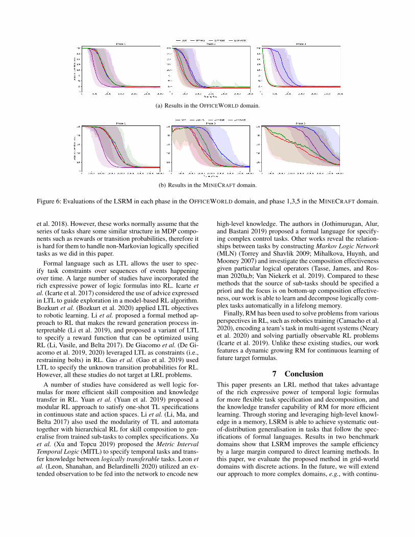
(a) Results in the OFFICEWORLD domain.

(b) Results in the MINECRAFT domain.

Figure 6: Evaluations of the LSRM in each phase in the OFFICEWORLD domain, and phase 1,3,5 in the MINECRAFT domain.

et al. 2018). However, these works normally assume that theseries of tasks share some similar structure in MDP compo-nents such as rewards or transition probabilities, therefore itis hard for them to handle non-Markovian logically specifiedtasks as we did in this paper.

Formal language such as LTL allows the user to spec-ify task constraints over sequences of events happeningover time. A large number of studies have incorporated therich expressive power of logic formulas into RL. Icarte etal. (Icarte et al. 2017) considered the use of advice expressedin LTL to guide exploration in a model-based RL algorithm.Bozkurt et al. (Bozkurt et al. 2020) applied LTL objectivesto robotic learning. Li et al. proposed a formal method ap-proach to RL that makes the reward generation process in-terpretable (Li et al. 2019), and proposed a variant of LTLto specify a reward function that can be optimized usingRL (Li, Vasile, and Belta 2017). De Giacomo et al. (De Gi-acomo et al. 2019, 2020) leveraged LTL as constraints (i.e.,restraining bolts) in RL. Gao et al. (Gao et al. 2019) usedLTL to specify the unknown transition probabilities for RL.However, all these studies do not target at LRL problems.

A number of studies have considered as well logic for-mulas for more efficient skill composition and knowledgetransfer in RL. Yuan et al. (Yuan et al. 2019) proposed amodular RL approach to satisfy one-shot TL specificationsin continuous state and action spaces. Li et al. (Li, Ma, andBelta 2017) also used the modularity of TL and automatatogether with hierarchical RL for skill composition to gen-eralise from trained sub-tasks to complex specifications. Xuet al. (Xu and Topcu 2019) proposed the Metric IntervalTemporal Logic (MITL) to specify temporal tasks and trans-fer knowledge between logically transferable tasks. Leon etal. (Leon, Shanahan, and Belardinelli 2020) utilized an ex-tended observation to be fed into the network to encode new

high-level knowledge. The authors in (Jothimurugan, Alur,and Bastani 2019) proposed a formal language for specify-ing complex control tasks. Other works reveal the relation-ships between tasks by constructing Markov Logic Network(MLN) (Torrey and Shavlik 2009; Mihalkova, Huynh, andMooney 2007) and investigate the composition effectivenessgiven particular logical operators (Tasse, James, and Ros-man 2020a,b; Van Niekerk et al. 2019). Compared to thesemethods that the source of sub-tasks should be specified apriori and the focus is on bottom-up composition effective-ness, our work is able to learn and decompose logically com-plex tasks automatically in a lifelong memory.

Finally, RM has been used to solve problems from variousperspectives in RL, such as robotics training (Camacho et al.2020), encoding a team’s task in multi-agent systems (Nearyet al. 2020) and solving partially observable RL problems(Icarte et al. 2019). Unlike these existing studies, our workfeatures a dynamic growing RM for continuous learning offuture target formulas.

7 ConclusionThis paper presents an LRL method that takes advantageof the rich expressive power of temporal logic formulasfor more flexible task specification and decomposition, andthe knowledge transfer capability of RM for more efficientlearning. Through storing and leveraging high-level knowl-edge in a memory, LSRM is able to achieve systematic out-of-distribution generalisation in tasks that follow the spec-ifications of formal languages. Results in two benchmarkdomains show that LSRM improves the sample efficiencyby a large margin compared to direct learning methods. Inthis paper, we evaluate the proposed method in grid-worlddomains with discrete actions. In the future, we will extendour approach to more complex domains, e.g., with continu-

ous states and/or actions.

ReferencesAbel, D.; Jinnai, Y.; Guo, S. Y.; Konidaris, G.; and Littman,M. 2018. Policy and value transfer in lifelong reinforcementlearning. In International Conference on Machine Learning,20–29. PMLR.Ammar, H. B.; Eaton, E.; Luna, J. M.; and Ruvolo, P. 2015.Autonomous cross-domain knowledge transfer in lifelongpolicy gradient reinforcement learning. In Twenty-FourthInternational Joint Conference on Artificial Intelligence.Andreas, J.; Klein, D.; and Levine, S. 2017. Modular multi-task reinforcement learning with policy sketches. In Interna-tional Conference on Machine Learning, 166–175. PMLR.Bacchus, F.; and Kabanza, F. 2000. Using temporal logicsto express search control knowledge for planning. Artificialintelligence, 116(1-2): 123–191.Bozkurt, A. K.; Wang, Y.; Zavlanos, M. M.; and Pajic, M.2020. Control synthesis from linear temporal logic speci-fications using model-free reinforcement learning. In 2020IEEE International Conference on Robotics and Automation(ICRA), 10349–10355. IEEE.Brunskill, E.; and Li, L. 2014. Pac-inspired option discoveryin lifelong reinforcement learning. In International confer-ence on machine learning, 316–324. PMLR.Camacho, A.; Icarte, R. T.; Klassen, T. Q.; Valenzano, R. A.;and McIlraith, S. A. 2019. LTL and Beyond: Formal Lan-guages for Reward Function Specification in ReinforcementLearning. In IJCAI, volume 19, 6065–6073.Camacho, A.; Varley, J.; Jain, D.; Iscen, A.; and Kalash-nikov, D. 2020. Disentangled Planning and Control in Vi-sion Based Robotics via Reward Machines. arXiv preprintarXiv:2012.14464.De Giacomo, G.; Favorito, M.; Iocchi, L.; and Patrizi, F.2020. Imitation learning over heterogeneous agents withrestraining bolts. In Proceedings of the International Con-ference on Automated Planning and Scheduling, volume 30,517–521.De Giacomo, G.; Iocchi, L.; Favorito, M.; and Patrizi, F.2019. Foundations for restraining bolts: Reinforcementlearning with LTLf/LDLf restraining specifications. InProceedings of the International Conference on AutomatedPlanning and Scheduling, volume 29, 128–136.Gao, Q.; Hajinezhad, D.; Zhang, Y.; Kantaros, Y.; and Za-vlanos, M. M. 2019. Reduced variance deep reinforcementlearning with temporal logic specifications. In Proceedingsof the 10th ACM/IEEE International Conference on Cyber-Physical Systems, 237–248.Garcia, F. M.; and Thomas, P. S. 2019. A meta-MDP ap-proach to exploration for lifelong reinforcement learning.arXiv preprint arXiv:1902.00843.Icarte, R. T.; Klassen, T.; Valenzano, R.; and McIlraith, S.2018. Using reward machines for high-level task specifica-tion and decomposition in reinforcement learning. In ICML,2107–2116.

Icarte, R. T.; Klassen, T. Q.; Valenzano, R.; and McIlraith,S. A. 2017. Using advice in model-based reinforcementlearning. In The 3rd Multidisciplinary Conference on Re-inforcement Learning and Decision Making (RLDM).Icarte, R. T.; Waldie, E.; Klassen, T.; Valenzano, R.; Cas-tro, M.; and McIlraith, S. 2019. Learning reward machinesfor partially observable reinforcement learning. In NeurIPS,15523–15534.Isele, D.; and Cosgun, A. 2018. Selective experience replayfor lifelong learning. In Proceedings of the AAAI Conferenceon Artificial Intelligence, volume 32.Jothimurugan, K.; Alur, R.; and Bastani, O. 2019. A Com-posable Specification Language for Reinforcement Learn-ing Tasks. In Advances in Neural Information ProcessingSystems 32: Annual Conference on Neural Information Pro-cessing Systems 2019, NeurIPS 2019.Leon, B. G.; Shanahan, M.; and Belardinelli, F. 2020.Systematic Generalisation through Task Temporal Logicand Deep Reinforcement Learning. arXiv preprintarXiv:2006.08767.Li, X.; Ma, Y.; and Belta, C. 2017. Automata-guided hier-archical reinforcement learning for skill composition. arXivpreprint arXiv:1711.00129.Li, X.; Serlin, Z.; Yang, G.; and Belta, C. 2019. A formalmethods approach to interpretable reinforcement learningfor robotic planning. Science Robotics, 4(37).Li, X.; Vasile, C.-I.; and Belta, C. 2017. Reinforcementlearning with temporal logic rewards. In 2017 IEEE/RSJInternational Conference on Intelligent Robots and Systems(IROS), 3834–3839. IEEE.Linz, P. 2006. An introduction to formal languages and au-tomata. Jones & Bartlett Learning.Mihalkova, L.; Huynh, T.; and Mooney, R. J. 2007. Mappingand revising markov logic networks for transfer learning. InAaai, volume 7, 608–614.Neary, C.; Xu, Z.; Wu, B.; and Topcu, U. 2020. Reward ma-chines for cooperative multi-agent reinforcement learning.arXiv preprint arXiv:2007.01962.Pnueli, A. 1977. The temporal logic of programs. In 18thAnnual Symposium on Foundations of Computer Science(sfcs 1977), 46–57. IEEE.Rolnick, D.; Ahuja, A.; Schwarz, J.; Lillicrap, T. P.; andWayne, G. 2018. Experience replay for continual learning.arXiv preprint arXiv:1811.11682.Rusu, A. A.; Rabinowitz, N. C.; Desjardins, G.; Soyer, H.;Kirkpatrick, J.; Kavukcuoglu, K.; Pascanu, R.; and Had-sell, R. 2016. Progressive neural networks. arXiv preprintarXiv:1606.04671.Schwarz, J.; Czarnecki, W.; Luketina, J.; Grabska-Barwinska, A.; Teh, Y. W.; Pascanu, R.; and Hadsell, R.2018. Progress & compress: A scalable framework for con-tinual learning. In International Conference on MachineLearning, 4528–4537. PMLR.Sutton, R. S.; and Barto, A. G. 2018. Reinforcement learn-ing: An introduction. MIT press.

Tasse, G. N.; James, S.; and Rosman, B. 2020a. A booleantask algebra for reinforcement learning. arXiv preprintarXiv:2001.01394.Tasse, G. N.; James, S.; and Rosman, B. 2020b. LogicalComposition in Lifelong Reinforcement Learning.Toro Icarte, R.; Klassen, T. Q.; Valenzano, R.; and McIlraith,S. A. 2018. Teaching multiple tasks to an RL agent usingLTL. In AAMAS, 452–461.Toro Icarte, R.; Klassen, T. Q.; Valenzano, R.; and McIlraith,S. A. 2020. Reward Machines: Exploiting Reward FunctionStructure in Reinforcement Learning. arXiv e-prints, arXiv–2010.Torrey, L.; and Shavlik, J. 2009. Policy transfer via Markovlogic networks. In International Conference on InductiveLogic Programming, 234–248. Springer.Van Niekerk, B.; James, S.; Earle, A.; and Rosman, B. 2019.Composing value functions in reinforcement learning. In In-ternational Conference on Machine Learning, 6401–6409.PMLR.Watkins, C. J.; and Dayan, P. 1992. Q-learning. Machinelearning, 8(3-4): 279–292.Xu, Z.; and Topcu, U. 2019. Transfer of Temporal LogicFormulas in Reinforcement Learning. In IJCAI: proceedingsof the conference, volume 28, 4010–4018.Yuan, L. Z.; Hasanbeig, M.; Abate, A.; and Kroening, D.2019. Modular deep reinforcement learning with temporallogic specifications. arXiv preprint arXiv:1909.11591.

A Full Definitions and Proofs of SLTLThe syntax of SLTL formulas differs from LTL in terms ofthe “then” operator, i.e.,

ϕ := p | ¬ϕ | ϕ ∧ ψ | ©ϕ | ϕUψ | ϕ ∼ ψ, p ∈ P. (5)

The semantic of the operator “then” is defined as

λ |= ϕ ∼ ψ ⇔

∃j ≥ 0, λ0:j |= ϕ, λj+1 |= ψ,

and ∀i < j, λ0:i 6|= ϕ, if ϕ 6= >;

λ |= ψ, if ϕ = >,(6)

where the notation λi:j denotes the sub sequencelili+1 · · · lj .

The SLTL progression of formulas composed by the“then” operator is defined as

prog(ϕ ∼ ψ, l) =

{prog(ϕ, l) ∼ ψ, if ϕ 6= >;

prog(ψ, l), if ϕ = >, (7)

whereϕ,ψ are SLTL formulas and l is a label. The followingtheorem theoretically ensures that the progression of SLTLis well defined.

Theorem 2. For all SLTL formula ϕ and a label sequencedenoted by λ, we have λi |= ϕ if and only if λi+1 |=prog(ϕ, li) for all i ≥ 0.

Proof. It has been proved for LTL formulas. Therefore,we only need to prove that λi |= ϕ ∼ ψ ⇔ λi+1 |=prog(ϕ ∼ ψ, li). If ϕ1 6= >, then λi |= ϕ1 ∼ ϕ2 ⇔∃j ≥ i, λi:j |= ϕ1, λ

j+1 |= ϕ2,∀t < j, λi:t 6|= ϕ1 ⇔λi+1:j |= prog(ϕ1, li) and λj |= ϕ2,∀t < j, λi+1:t 6|=prog(ϕ1, li) ⇔ λi+1 |= prog(ϕ1, li) ∼ ϕ2 = prog(ϕ1 ∼ϕ2, li). If ϕ1 = >, then λi |= ϕ1 ∼ ϕ2 = ϕ2 ⇔ λi+1 |=prog(ϕ2, li) = prog(ϕ1 ∼ ϕ2, li).

Finally, we give the proofs of operator laws in the follow-ing.Theorem 3. For any SLTL formulas ϕ1, ϕ2, ϕ3, we haveassociative law: (ϕ1 ∼ ϕ2) ∼ ϕ3 = ϕ1 ∼ (ϕ2 ∼ ϕ3),and distribution laws (i)(ϕ1 ∼ ϕ2) ∧ (ϕ1 ∼ ϕ3) = ϕ1 ∼(ϕ2 ∧ ϕ3); (ii)(ϕ1 ∼ ϕ3) ∧ (ϕ2 ∼ ϕ3) = (ϕ1 ∧ ϕ2) ∼ ϕ3;(iii)(ϕ1 ∼ ϕ2) ∨ (ϕ1 ∼ ϕ3) = ϕ1 ∼ (ϕ2 ∨ ϕ3); and(iv)(ϕ1 ∼ ϕ3) ∨ (ϕ2 ∼ ϕ3) = (ϕ1 ∨ ϕ2) ∼ ϕ3.

Proof. We first prove the associative law. We have λ |=(ϕ1 ∼ ϕ2) ∼ ϕ3 ⇔ ∃0 ≤ i < j, λ0:i |= ϕ1, λ

i+1:j |=ϕ2, λ

j |= ϕ3 ⇔ λ |= ϕ1 ∼ (ϕ2 ∼ ϕ3). Hence, (ϕ1 ∼ϕ2) ∼ ϕ3 = ϕ1 ∼ (ϕ2 ∼ ϕ3).

We then prove the distribution law (i). λ |= (ϕ1 ∼ϕ2) ∧ (ϕ1 ∼ ϕ3) ⇔ ∃i, j ≥ 0, λ0:i |= ϕ1, λ

i+1 |=ϕ2, λ

0:j |= ϕ1, λj+1 |= ϕ2 and∀k < min{i, j}, λ0:k 6|=

ϕ1 ⇔ λ0:min{i,j} |= ϕ1, λmin{i,j} |= ϕ2 ∧ ϕ3 ⇔ λ |=

ϕ1 ∼ (ϕ2 ∧ ϕ3). Hence, (ϕ1 ∼ ϕ2) ∧ (ϕ1 ∼ ϕ3) = ϕ1 ∼(ϕ2 ∧ ϕ3). The proofs of (ii)-(iv) are similar.

B Experimental SettingsThe source tasks and target tasks in Section 5.1 are listed inTable 1 and 2, respectively.

In Section 5.2, the target task is “delivering coffee andmail to office avoiding furniture” in the OFFICEWORLD do-main. Its smallest representation is [(¬ ∗ Uc) ∼ (¬ ∗ Uo)] ∧[(¬ ∗ Um) ∼ (¬ ∗ Uo)], and the other representation is[(¬ ∗ Uc) ∧ (¬ ∗ Um)] ∼ (¬ ∗ Uo) (see Figure 7). In theMINECRAFT domain, the target task is “making bed”, andits smallest representation is [(♦a ∼ ♦b) ∧ ♦d] ∼ (♦c),while the other representations are [(♦a ∼ ♦b) ∼ ♦c] ∧(♦d ∼ ♦c) and [♦a ∼ (♦b ∼ ♦c)] ∧ (♦d ∼ ♦c) (see Fig-ure 8).

In Section 5.3, the sequences of tasks in each phase in thetwo domains are listed in Table 3 and 4, respectively.

C Illustrations of the LSRM Processes in theExperiments

Figure 9 and 10 give illustrations of LSRM processes inthe OFFICEWORLD and MINECRAFT domain, respectively.The nodes (rectangles) encoded with SLTL formulas arestates in RM, and the black solid arrows are the transitionsamong them. Formulas colored in white have already beenlearned before, while formulas colored in red have not beenlearned. The red dotted arrows represent the Q-functionstransferred from the learned formulas to the correspondingtarget formulas.

Domain Source Task SLTL Formula

OFFICEWORLD

deliver coffee to office avoiding furniture ϕ1 = (¬ ∗ Uc) ∼ (¬ ∗ Uo)deliver mail to office avoiding furniture ϕ2 = (¬ ∗ Um) ∼ (¬ ∗ Uo)go to B then office avoiding furniture ϕ3 = (¬ ∗ UB) ∼ (¬ ∗ Uo)

go to B then C avoiding furniture ϕ4 = (¬ ∗ UB) ∼ (¬ ∗ UC)go to office then B avoiding furniture ϕ5 = (¬ ∗ Uo) ∼ (¬ ∗ UB)

get mail then go to D avoiding furniture ϕ6 = (¬ ∗ Um) ∼ (¬ ∗ UD)get mail then go to A avoiding furniture ϕ7 = (¬ ∗ Um) ∼ (¬ ∗ UA)

MINECRAFT

make plank ψ1 = (♦a) ∼ (♦b)make stick ψ2 = (♦a) ∼ (♦c)make cloth ψ3 = (♦d) ∼ (♦e)make rope ψ4 = (♦d) ∼ (♦b)

make bridge ψ5 = (♦a ∧ ♦f) ∼ (♦e)make shears ψ6 = (♦a ∧ ♦f) ∼ (♦c)

Table 1: Source tasks in the two domains.

Domain Target Task SLTL Formula

OFFICEWORLD

complete source task 1 and 2 ϕ1 ∧ ϕ2

complete source task 4 and 6 ϕ4 ∧ ϕ6

complete source task 4 or 5 ϕ4 ∨ ϕ5

complete source task 4 or 7 ϕ4 ∨ ϕ7

complete source task 4 then 5 ϕ4 ∼ ϕ5

complete source task 4 then 6 ϕ4 ∼ ϕ6

complete source task 5 then 6 ϕ5 ∼ ϕ6

MINECRAFT

complete source task 1 and 3 ψ1 ∧ ψ3

complete source task 4 and 5 ψ4 ∧ ψ5

complete source task 4 and 6 ψ4 ∧ ψ6

complete source task 1 or 3 ψ1 ∨ ψ3

complete source task 2 or 3 ψ2 ∨ ψ3

complete source task 2 then 3 ψ2 ∼ ψ3

complete source task 5 then 6 ψ5 ∼ ψ6

Table 2: Target tasks in the two domains.

Figure 7: Representations of the task “delivering coffee and mail to office avoiding furniture” in the OFFICEWORLD domain.

Figure 8: Representations of the task “making bed” in the MINECRAFT domain

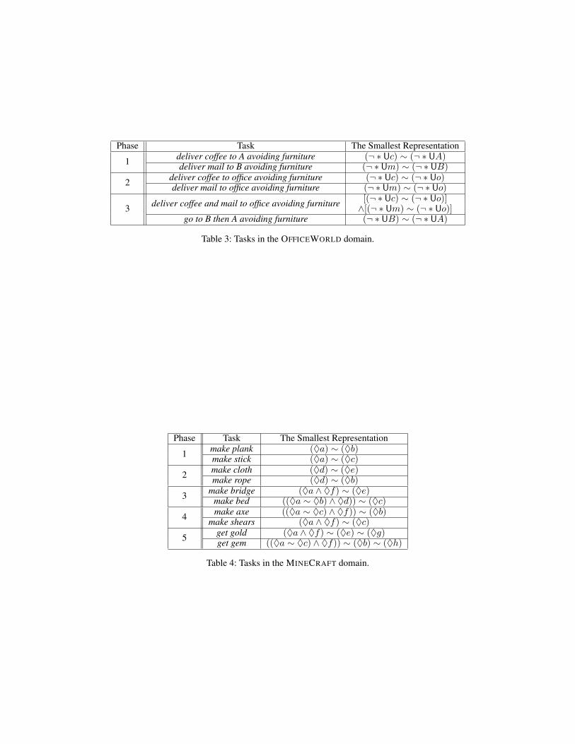
Phase Task The Smallest Representation

1 deliver coffee to A avoiding furniture (¬ ∗ Uc) ∼ (¬ ∗ UA)deliver mail to B avoiding furniture (¬ ∗ Um) ∼ (¬ ∗ UB)

2 deliver coffee to office avoiding furniture (¬ ∗ Uc) ∼ (¬ ∗ Uo)deliver mail to office avoiding furniture (¬ ∗ Um) ∼ (¬ ∗ Uo)

3 deliver coffee and mail to office avoiding furniture [(¬ ∗ Uc) ∼ (¬ ∗ Uo)]∧[(¬ ∗ Um) ∼ (¬ ∗ Uo)]

go to B then A avoiding furniture (¬ ∗ UB) ∼ (¬ ∗ UA)

Table 3: Tasks in the OFFICEWORLD domain.

Phase Task The Smallest Representation

1 make plank (♦a) ∼ (♦b)make stick (♦a) ∼ (♦c)

2 make cloth (♦d) ∼ (♦e)make rope (♦d) ∼ (♦b)

3 make bridge (♦a ∧ ♦f) ∼ (♦e)make bed ((♦a ∼ ♦b) ∧ ♦d)) ∼ (♦c)

4 make axe ((♦a ∼ ♦c) ∧ ♦f)) ∼ (♦b)make shears (♦a ∧ ♦f) ∼ (♦c)

5 get gold (♦a ∧ ♦f) ∼ (♦e) ∼ (♦g)get gem ((♦a ∼ ♦c) ∧ ♦f)) ∼ (♦b) ∼ (♦h)

Table 4: Tasks in the MINECRAFT domain.

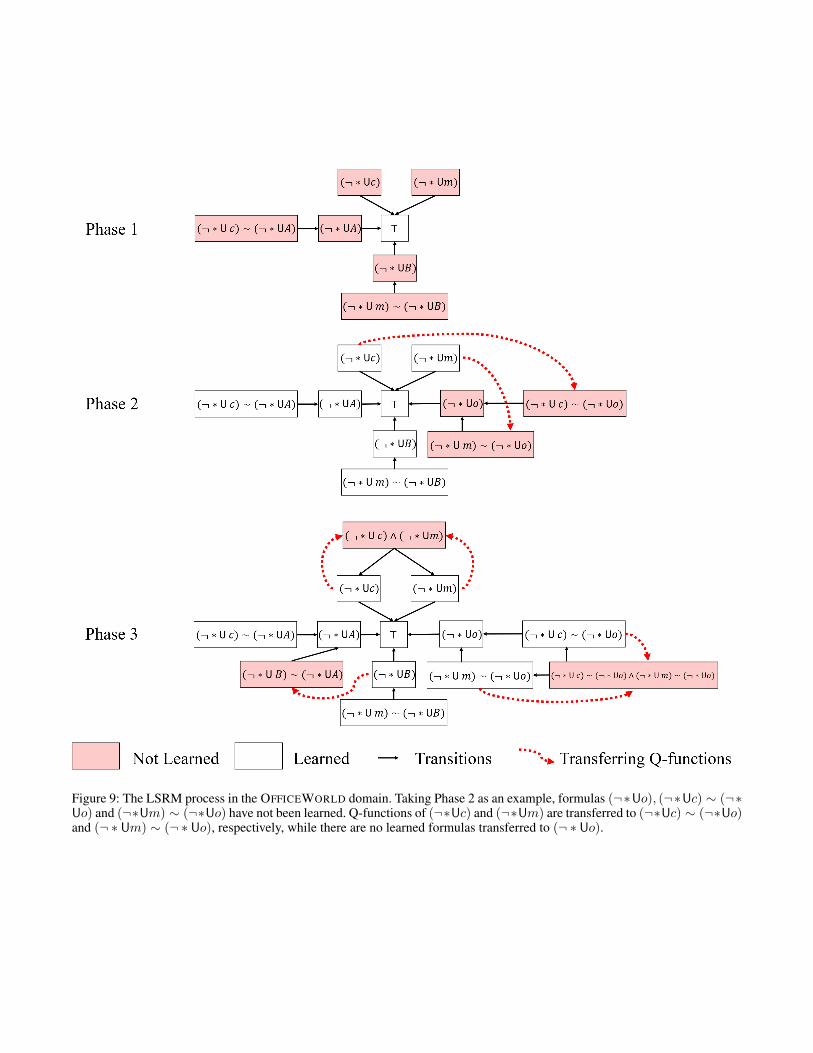
Figure 9: The LSRM process in the OFFICEWORLD domain. Taking Phase 2 as an example, formulas (¬∗Uo), (¬∗Uc) ∼ (¬∗Uo) and (¬∗Um) ∼ (¬∗Uo) have not been learned. Q-functions of (¬∗Uc) and (¬∗Um) are transferred to (¬∗Uc) ∼ (¬∗Uo)and (¬ ∗ Um) ∼ (¬ ∗ Uo), respectively, while there are no learned formulas transferred to (¬ ∗ Uo).

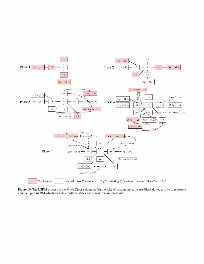
Figure 10: The LSRM process in the MINECRAFT domain. For the sake of succinctness, we use black dotted arrows to representa hidden part of RM which includes multiple states and transitions in Phase 4-5.