limited-angle cone-beam computed tomography image

J. Inverse Ill-Posed Probl. 21 (2013), 735–754DOI 10.1515/ jip-2011-0010 © de Gruyter 2013

Limited-angle cone-beam computed tomographyimage reconstruction by total variation

minimization and piecewise-constant modification

Li Zeng, Jiqiang Guo and Baodong Liu

Abstract. Because of x-ray dose considerations or practical mechanical restrictions, it maybe interesting for some applications to perform limited-angle scanning. So the limited-angle problem is of practical significance in computed tomography (CT). Furthermore,it is an ill-posed problem. Total variation minimization (TVM) and projection on con-vex sets (POCS) based iterative reconstruction algorithm is comparatively valid for thisundersampling CT reconstruction problem and can obtain comparatively good perfor-mance. But the reconstruction images have artifacts with gradual change gray nearbyedges. In this paper, a simple but efficient method to eliminate such artifacts during thereconstruction is proposed. Based on the same assumption of the TVM algorithm, forthe object whose density distribution is approximate piecewise-constant, we develop andinvestigate an improved iterative reconstruction algorithm for volume image reconstruc-tion from limited-angle cone-beam scan, which is referred to as piecewise-constant mod-ification TVM-POCS (PM-TVM-POCS) algorithm. The grays of voxels with graduallychanged gray artifacts are modified in the TVM-POCS iteration process by the piecewise-constant modification algorithm which is regarded as a “collapse” process, and graduallyapproaches the true piecewise-constant image. The results of simulation experiments showthat the presented modification algorithm can improve the quality of the reconstructed im-age obviously and it is steady to noise. This modification algorithm can also be applied toother reconstruction problems which have artifacts with gradual change gray.

Keywords. Cone-beam computed tomography, limited-angle, ill-posed problem, totalvariation minimization, piecewise-constant modification.

2010 Mathematics Subject Classification. 92C55.

1 Introduction

Because the circular cone-beam imaging systems is a technically simple CT con-figuration to implement and the longitude resolution of the reconstruction imageis high, it is widely used in many CT applications, such as screening for breast tu-mors or lung cancer [1,2,23], image guided radiation therapy [13], C-arm scanning

This work is supported by the National Natural Science Foundation of China (Grant No. 60972104).

736 L. Zeng, J. Guo and B. Liu

for angiography or intraoperative tomographic imaging [7], and micro-CT [11]. Inthe use of CT for medical diagnosis, it may be extremely important to minimizethe dose of the x-ray from CT scan. Because the radiation dose of CT imaging tothe patient poses a serious radiation safety concern, studies indicate that the doseof x-ray radiation from CT scans may have a lifetime attributable risk of cancer tothe patient [10,19]. Reducing CT dose has been an area of active research in med-ical imaging. An available way of reducing CT x-ray scanning radiation dose is todecrease the sampling projection view range. In industrial CT, because of practicalconstraints due to the imaging hardware or scanning geometry, in some cases thex-ray source and detector (or the scanned object relatively) only can continuouslyrotate limited-angle range.

Therefore, for x-ray dose considerations or practical mechanical restrictions, itmay be interesting for some CT applications to perform limited-angle scanningwhich is referred to as the limited-angle CT. Undoubtedly, reducing sampling pro-jection view range can speed up the reconstruction rate. However, it leads to achallenging image reconstruction task. Since samples are limited, the task of re-covering the image would involve solving an underdetermined matrix equation,that is, there is a huge quantity of candidate images that all can fit the limited mea-surements effectively. Thus, some additional constraints are needed to select the“best” candidate. In the past few years, several algorithms were proposed to over-come the data insufficient reconstruction problem in tomographic imaging withvarying degrees of success [8, 15, 21].

The classical method to such problems is to minimize the `2-norm of the re-constructed image. However, Donoho and Tao’s groups [3, 9] showed that findingthe “best” candidate with the minimum `1-norm of the reconstructed image, alsoequivalent to the total variation minimization (TVM) in some cases [16], is themore reasonable choice. The insufficient projection data CT reconstruction prob-lem can be expressed as a linear program and solved efficiently using existingmethods. Motivated by this theoretic result, Sidky and Pan [17, 18] developedand investigated an iterative image reconstruction algorithm based on the POCSalgorithm and the TVM method to the undersampling and insufficient data CT im-age reconstruction problems. This algorithm can be called TVM-POCS algorithmfor short. It supposes that the gray (corresponding density) of the imaged objectis piecewise-constant, so the gradient magnitude image of the object is sparse.Then by way of minimizing the total variation (TV) of the image, subject to theconstraint that the estimated projection data is within a specified tolerance of theavailable measurement data and the reconstruction values of the image are non-negative to obtain the reconstruction image. This algorithm is comparatively validfor this undersampling CT reconstruction problem and can obtain comparativelygood reconstruction images.

Limited-angle cone-beam computed tomography image reconstruction 737

However, for the limited-angle cone-beam CT reconstruction problem dis-cussed in this paper, our studies show that the reconstructed images (for exam-ple, the 3D Shepp–Logan phantom and an automobile hub) by the TVM-POCSalgorithm have artifacts with gradual change gray in some regions (for example,some regions near edges, see Section 4). For convenience, we simply refer tothese regions as insufficient reconstruction regions throughout this paper. In the in-sufficient reconstruction region, the reconstructed image has gradual change grayvalue, which is not in accord with the practical density information of the imagedobject.

In practical application cases, many biomedical images can be approximatelymodeled as being piecewise-constant [4,20]. This is because the x-ray attenuationcoefficient often varies mildly within organs, and large image variations areas areusually confined to the borders of tissue structures. A sparse gradient image mayalso be a good image model in industrial or security applications [22]. So, based onthe same hypothesis of the TVM algorithm, namely, the density distribution of theimaged object is approximately piecewise-constant, we develop and investigate apiecewise-constant modification algorithm, and introduce it into the TVM-POCSalgorithm to obtain a modified iterative reconstruction algorithm for volume im-age reconstruction from limited-angle cone-beam scan data, which is referred toas PM-TVM-POCS algorithm. Experimental results show that the presented algo-rithm can solve the problem of insufficient reconstruction region of TVM-POCSand improve the quality of the reconstructed image significantly. Although in somesense, the piecewise-constant modification algorithm is a heuristic approach, it iseffective. Furthermore, the presented algorithm is robust to noise. Apparently, thismodification method can be applied to other reconstruction problems which haveartifacts with gradual change gray.

The rest of this paper is organized as follows. In Section 2, the geometry con-figuration of circular cone-beam CT is illustrated. In Section 3, we describe ourmodified iterative algorithm for tomographic image reconstruction from limited-angle cone-beam scanning projection data. In Section 4, numeric experimental re-sults are employed to demonstrate the usefulness and advantage of our algorithm.Finally, a conclusion is provided in Section 5.

2 Circular cone-beam CT geometry configuration andprojection data acquisition

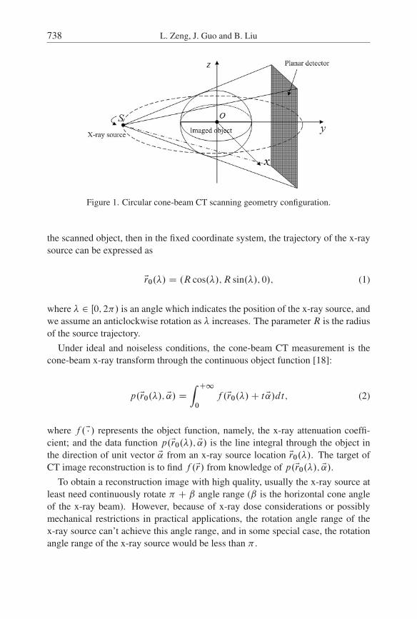
Figure 1 is the circular cone-beam CT scanning geometry configuration used inthis paper. The x-ray source motion trajectory is considered as a circle. If weintroduce a 3D Cartesian coordinate system (x; y; z) that is fixed on the center of


Figure 1. Circular cone-beam CT scanning geometry configuration.

the scanned object, then in the fixed coordinate system, the trajectory of the x-raysource can be expressed as

Er0.�/ D .R cos.�/; R sin.�/; 0/; (1)

where � 2 Œ0; 2�/ is an angle which indicates the position of the x-ray source, andwe assume an anticlockwise rotation as � increases. The parameter R is the radiusof the source trajectory.

Under ideal and noiseless conditions, the cone-beam CT measurement is thecone-beam x-ray transform through the continuous object function [18]:

p.Er0.�/; E/ D

Z C10

f .Er0.�/C t E/dt; (2)

where f .E� / represents the object function, namely, the x-ray attenuation coeffi-cient; and the data function p.Er0.�/; E/ is the line integral through the object inthe direction of unit vector E from an x-ray source location Er0.�/. The target ofCT image reconstruction is to find f .Er/ from knowledge of p.Er0.�/; E/.

To obtain a reconstruction image with high quality, usually the x-ray source atleast need continuously rotate � C ˇ angle range (ˇ is the horizontal cone angleof the x-ray beam). However, because of x-ray dose considerations or possiblymechanical restrictions in practical applications, the rotation angle range of thex-ray source can’t achieve this angle range, and in some special case, the rotationangle range of the x-ray source would be less than � .


3 Method

3.1 CT system discretization

The imaging CT system can be approximated by the following discrete linear sys-tem [12]:

W Ef D Ep; (3)

where Ef D Œf1; f2; : : : ; fN �T 2 RN represents the object function of length

N , Ep D Œp1; p2; : : : ; pM �T 2 RM is the projection data vector with individual

measurement referred to as pi (i D 1; 2; : : : ;M ), andW is the system matrix withsize of M �N which is a discrete model for the integration in equation (2).

The image reconstruction problem is equivalent to inverting the linear system(3), finding Ef from a projection data set Ep. For the problem of limited-angle CTreconstruction, the number of projection data M is far from abundant to uniquelydetermine the N values of the object function vector Ef by directly inverting equa-tion (3), namely, the system matrix W is serious ill-posed.

3.2 TVM algorithm

The TV of the 3D image depends on the variation of the image over neighboringvoxels, and to formulate the image TV a three index notation for the image voxelsis required. If we indicate the gray of the 3D image Ef at voxel .k; s; t/ as fk;s;t(k D 1; 2; : : : ; Nk , s D 1; 2; : : : ; Ns , and t D 1; 2; : : : ; Nt , where Nk , Ns , andNt are the numbers of voxels along each of the images axes), then the gradientmagnitude of the voxel .k; s; t/ can be denoted as [14]

jrfk;s;t j D

q.fk;s;t �fk�1;s;t /

2 C .fk;s;t �fk;s�1;t /2 C .fk;s;t �fk;s;t�1/

2:

This quantity is referred to as the gradient image. The `1-norm of the gradientimage, also equivalent to the TV of the image, is defined as

k Ef kTV DXk;s;t

q.fk;s;t �fk�1;s;t /

2 C .fk;s;t �fk;s�1;t /2 C .fk;s;t �fk;s;t�1/

2:

Essentially, the TVM algorithm is an optimization program problem by minimiz-ing the `1-norm of the gradient image, which yields possibly the exact image forsparse data problems under the condition of exact data consistency. However, inpractical situations, the projection data often contain some form of inconsistency.The digital measurements may contain noise, and the discrete, linear cone-beamtransform is only an approximate model for the projection data that are measured.


To account for the data inconsistencies, the optimization problem can be expressedas [18]

Ef � D arg mink Ef kTV such that jW Ef � � Epj � " and Ef � � 0; (4)

where Ef � is the “best” reconstruction image and " is the level data inconsistencytolerance parameter.

Sidky, Kao and Pan [17] showed that the TVM method is very efficient in imagereconstruction from sparse or limited-angle data. Furthermore, it can smooth outnoise in the image while preserving edges within the image. They developed aTVM-POCS iterative algorithm to solve the optimization problem above. Moredetails can be found in [17].

The TVM-POCS algorithm to data acquired with sparsely sampled view-anglescan obtain very good performance. However, for the limited-angle problem wediscussed, the reconstructed images have artifacts with insufficient reconstruc-tion regions. In the insufficient reconstruction region, the reconstructed image hasgradual change gray, which is not in accord with the practical density informationof the imaged object.

3.3 Piecewise-constant modification algorithm

To solve the problem of gradual change gray artifacts in the reconstruction im-ages by the TVM-POCS algorithm, in this paper, a heuristic approach is devel-oped, which is called as piecewise-constant modification algorithm. The aimof the piecewise-constant modification algorithm is to modify the regions withgradual change gray to piecewise-constant regions. For easily understanding, thepiecewise-constant modification algorithm can be regarded as a “collapse” pro-cess. The gradual change region voxel flows to neighborly lower gray voxels by“collapse”, gradually it approaches a piecewise-constant region. For the sake ofbriefness and avoiding repeated computation, we only consider the case of outflowof each voxel with gradual change gray. Although after the piecewise-constantmodification the gray of some regions may become higher than that of the imageitself, and it will bring the inconsistency of digital measurements projection, thiscan be successfully settled by way of TVM-POCS iteration. Because if only thereis piecewise-constant modification, after that it will carry out some TVM-POCSiterations to obtain the final reconstruction image.

If we define the mass of a 3D image to be the sum of all voxel densities, it iseasy to see that the sum of projection data of each view angle equals the mass ofthe image. So, the piecewise-constant modification algorithm maintains the massconstantly. Besides, the edges or contours are important characteristics of images,they must be preserved in the process of piecewise-constant modification.


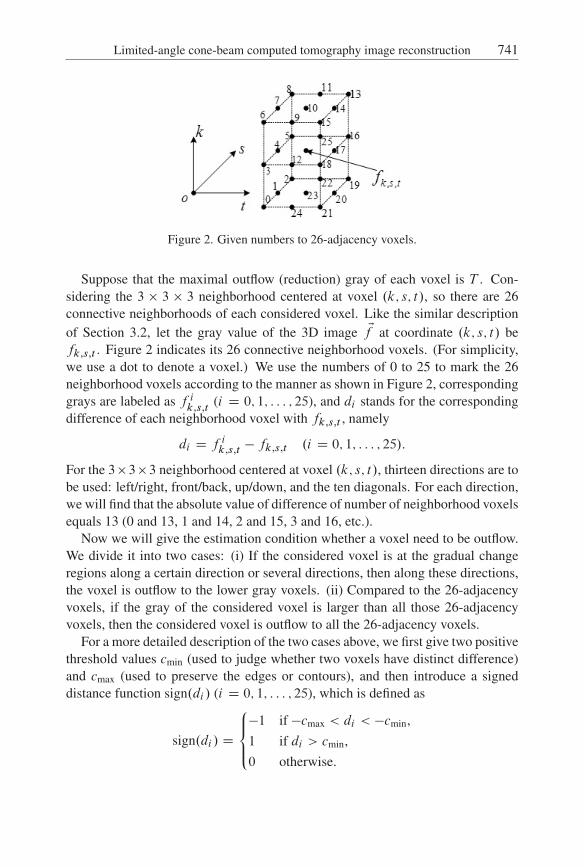
Figure 2. Given numbers to 26-adjacency voxels.

Suppose that the maximal outflow (reduction) gray of each voxel is T . Con-sidering the 3 � 3 � 3 neighborhood centered at voxel .k; s; t/, so there are 26connective neighborhoods of each considered voxel. Like the similar descriptionof Section 3.2, let the gray value of the 3D image Ef at coordinate .k; s; t/ befk;s;t . Figure 2 indicates its 26 connective neighborhood voxels. (For simplicity,we use a dot to denote a voxel.) We use the numbers of 0 to 25 to mark the 26neighborhood voxels according to the manner as shown in Figure 2, correspondinggrays are labeled as f i

k;s;t(i D 0; 1; : : : ; 25), and di stands for the corresponding

difference of each neighborhood voxel with fk;s;t , namely

di D fik;s;t � fk;s;t .i D 0; 1; : : : ; 25/:

For the 3�3�3 neighborhood centered at voxel .k; s; t/, thirteen directions are tobe used: left/right, front/back, up/down, and the ten diagonals. For each direction,we will find that the absolute value of difference of number of neighborhood voxelsequals 13 (0 and 13, 1 and 14, 2 and 15, 3 and 16, etc.).

Now we will give the estimation condition whether a voxel need to be outflow.We divide it into two cases: (i) If the considered voxel is at the gradual changeregions along a certain direction or several directions, then along these directions,the voxel is outflow to the lower gray voxels. (ii) Compared to the 26-adjacencyvoxels, if the gray of the considered voxel is larger than all those 26-adjacencyvoxels, then the considered voxel is outflow to all the 26-adjacency voxels.

For a more detailed description of the two cases above, we first give two positivethreshold values cmin (used to judge whether two voxels have distinct difference)and cmax (used to preserve the edges or contours), and then introduce a signeddistance function sign.di / (i D 0; 1; : : : ; 25), which is defined as

sign.di / D

8<:�1 if �cmax < di < �cmin,1 if di > cmin,0 otherwise.


So, case (i) can be denoted as

9i 2 ¹0; 1; : : : ; 12º such that sign.di / � sign.diC13/ D �1: (5)

Suppose the numbered voxel i satisfies equation (5), and sign.di / D �1, thenthe numbered voxel of acceptance outflow is i , otherwise the numbered voxel ofacceptance outflow is i C 13. Case (ii) can be denoted as:

8i 2 ¹0; 1; : : : ; 25º W sign.di / D �1:

From the above description we know that if the difference between two voxels isdistinct (the absolute value of the difference is not less than cmax/, then it is notoutflow along this direction which can avoid smoothing the edge or contour.

After it has confirmed the outflow direction of the considered voxel, we will givethe outflow rule. Suppose the numbers of all voxels of acceptance inflow composea set S � ¹0; 1; : : : ; 25º, then the sum of difference of all voxels in S with fk;s;t isPi2S di . According to the previous suppose that the maximal outflow (reduction)

gray of the considered voxel is T , so there will also be two cases:(i) If the inequality

2T CXi2S

di < 0

holds (namely, the outflow quantity achieves the maximal outflow value T ), thenit means that the outflow quantity is not enough to fill up the difference of fk;s;twith all voxels of S . Here, the gray of the considered voxel becomes fk;s;t � T .The increase quantity �i for each voxel of S is given by the formula

�i D Tdi=Xi2S

di :

(ii) If the inequality

2T CXi2S

di � 0

holds (namely, the outflow quantity is not more than the maximal outflow valueT ), then the grays of the considered voxel and all voxels of S are equal to�

fk;s;t CXi2S

f ik;s;t

�ı.jS j C 1/;

where jS j is the total element count of set S .


3.4 TVM and piecewise-constant modification based algorithm forlimited-angle cone-beam CT

Having introduced the piecewise-constant modification algorithm, now we de-scribe the steps of the presented iterative algorithm, which implements the opti-mization program described in equation (4) for image reconstruction from limited-angle cone-beam projection data and can be referred to as PM-TVM-POCS algo-rithm. Each iteration of the presented algorithm can be divided into three steps:(I) POCS-step, which can be further broken down into two steps: (a) data-step,which uses the simultaneous algebraic reconstruction technique (SART) [12] toenforce consistency with the projection data; (b) positivity constrain-step, whichconstrains the gray values of all reconstructed voxels to nonnegative; (II) TVM-step, which reduces the TV of the image estimate; and (III) PM-step, which intro-duces a piecewise-constant constrain as a penalty term into the iterative process,modifies the regions with gradual change gray to the piecewise-constant regions.

The detailed steps of the presented algorithm are as follows:

1. Initializing the reconstruction parameters: maximal iterative number Ncount,TVM-POCS iterative number for obtaining the initialization reconstruction im-ageNTVM-POCS, TV gradient descent algorithm step size a and iterative numberNgrad, interval of piecewise-constant modification iterative number Npc, max-imal outflow (reduction) gray of each voxel is T , cmin (used to judge whethertwo voxels have distinct difference) and cmax (used to preserve the edges orcontours). Let both the circulating counter l and the initialization value Ef .0/ ofthe reconstructed image be 0.

2. Data step: using the simultaneous algebraic reconstruction technique (SART)to reconstruct the image, for n D 1; 2; : : : ; N' , do

f.n/j D f

.n�1/j C �.n/

1Pi2�n

wij

Xi2�n

pi � QpiPNkD1w

2ik

wij ; j D 1; 2; : : : ; N;

where N' is the number of sampling projection views, �.n/ are the relaxationparameters which are all equal to 1 in our simulation experiment of Section 4,and �n indicates all projection data of the nth sampling projection view.

3. Nonnegative constraint step:

f.POCS/j D

´f.N'/

j f.N'/

j > 0;

0 otherwise,j D 1; 2; : : : ; N:


If l D Ncount � 1 or jW Ef .POCS/ � Epj � " (where " is the level data incon-sistency tolerance parameter), then output Ef .POCS/ as the final reconstructionimage; otherwise turn to next step.

4. TV gradient descent initialization:

dA D Ef .0/ � Ef .POCS/

2; Ef .TV-GRAD/

D Ef .POCS/:

5. TVM method, for i D 1; 2; : : : ; Ngrad, do

Ev.i/

k;s;tD@k Ef kTV

@fk;s;t

ˇfk;s;tDf

.TV-GRAD/

k;s;t

;

Ov.i/ D Ev.i/

k;s;t=jEv

.i/

k;s;tj;

Ef .TV-GRAD/D Ef .TV-GRAD/

� adA Ov.i/:

6. PM-step: if l � NTVM-POCS and l mod NPC D 0, proceed the piecewise-constant modification to obtain Ef .PC/.

7. Initializing the next loop: If l � NTVM-POCS and l mod NPC D 0, initializethe next loop by Ef .0/ D Ef .PC/; otherwise initialize the next loop by Ef .0/ DEf .TV-GRAD/. Let l D l C 1, turn to step 2.

The piecewise-constant modification step is controlled by the parametersNTVM-POCS and NPC. From the steps of the above-described algorithm we knowthat it doesn’t carry through the piecewise-constant modification for each iteration.First, it must carry throughNTVM-POCS times TVM-POCS iterations to gain a com-paratively good image, and then implement the piecewise-constant modification.Because of the piecewise-constant modification, it brings discrepancy between theprojection data of the reconstructed image with the original measurement projec-tion data, it must improve via some TVM-POCS iterations to ensure the consis-tency of projection data. So the interval of piecewise-constant modification is setto NPC. And the time of piecewise-constant modification is far less than the iter-ative time of the TVM-POCS algorithm, so the run time of the PM-TVM-POCSalgorithm is approximately equivalent to that of the TVM-POCS algorithm. Themeanings of other parameters are the same as those of the TVM-POCS algorithm,please refer to [17] for more detail.

4 The numerical simulation experiment results and discussion

To verify the effectiveness and advantage of the presented algorithm, we imple-mented it on a PC (2.4 GHz CPU, 4.0 G memory) coded in C++. The modified


No Center of the ellipsoid Semi-axes length Rotationangle

Attenuationcoefficient

1 .0:00; 0:00; 0:00/ .0:690; 0:920; 0:900/ 0 0.152 .0:00; 0:00; 0:00/ .0:662; 0:874; 0:880/ 0 �0:10

3 .�0:22; 0:000;�0:250/ .0:410; 0:160; 0:210/ 108 �0:05

4 .0:22; 0:000;�0:250/ .0:310; 0:110; 0:220/ 72 �0:05

5 .0:00; 0:350;�0:250/ .0:210; 0:250; 0:500/ 0 0.056 .0:00; 0:100;�0:250/ .0:046; 0:046; 0:046/ 0 0.057 .�0:08;�0:650;�0:250/ .0:046; 0:023; 0:020/ 0 0.058 .0:06;�0:650;�0:250/ .0:046; 0:023; 0:020/ 90 0.039 .0:06;�0:105; 0:625/ .0:056; 0:040; 0:100/ 90 0.03

10 .0:00; 0:100; 0:625/ .0:056; 0:056; 0:100/ 0 0.03

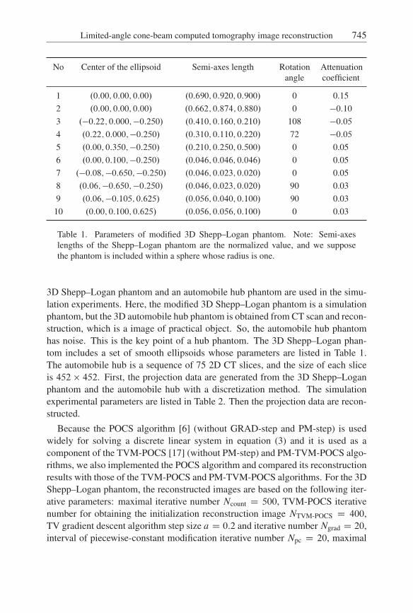
Table 1. Parameters of modified 3D Shepp–Logan phantom. Note: Semi-axeslengths of the Shepp–Logan phantom are the normalized value, and we supposethe phantom is included within a sphere whose radius is one.

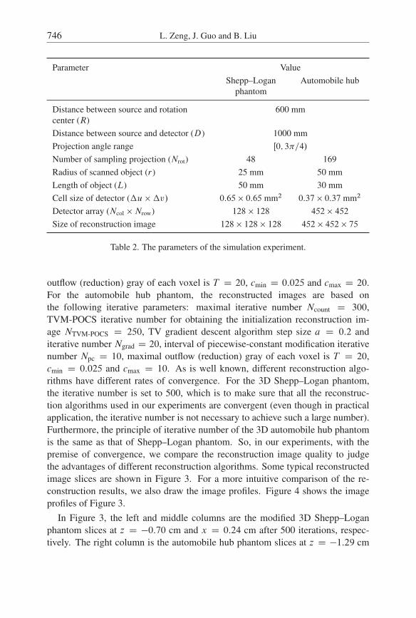
3D Shepp–Logan phantom and an automobile hub phantom are used in the simu-lation experiments. Here, the modified 3D Shepp–Logan phantom is a simulationphantom, but the 3D automobile hub phantom is obtained from CT scan and recon-struction, which is a image of practical object. So, the automobile hub phantomhas noise. This is the key point of a hub phantom. The 3D Shepp–Logan phan-tom includes a set of smooth ellipsoids whose parameters are listed in Table 1.The automobile hub is a sequence of 75 2D CT slices, and the size of each sliceis 452 � 452. First, the projection data are generated from the 3D Shepp–Loganphantom and the automobile hub with a discretization method. The simulationexperimental parameters are listed in Table 2. Then the projection data are recon-structed.

Because the POCS algorithm [6] (without GRAD-step and PM-step) is usedwidely for solving a discrete linear system in equation (3) and it is used as acomponent of the TVM-POCS [17] (without PM-step) and PM-TVM-POCS algo-rithms, we also implemented the POCS algorithm and compared its reconstructionresults with those of the TVM-POCS and PM-TVM-POCS algorithms. For the 3DShepp–Logan phantom, the reconstructed images are based on the following iter-ative parameters: maximal iterative number Ncount D 500, TVM-POCS iterativenumber for obtaining the initialization reconstruction image NTVM-POCS D 400,TV gradient descent algorithm step size a D 0:2 and iterative number Ngrad D 20,interval of piecewise-constant modification iterative number Npc D 20, maximal


Parameter ValueShepp–Logan

phantomAutomobile hub

Distance between source and rotationcenter (R)

600 mm

Distance between source and detector (D) 1000 mmProjection angle range Œ0; 3�=4/

Number of sampling projection (Nrot) 48 169Radius of scanned object (r) 25 mm 50 mmLength of object (L) 50 mm 30 mmCell size of detector (�u ��v/ 0:65 � 0:65 mm2 0:37 � 0:37 mm2

Detector array (Ncol �Nrow) 128 � 128 452 � 452

Size of reconstruction image 128 � 128 � 128 452 � 452 � 75

Table 2. The parameters of the simulation experiment.

outflow (reduction) gray of each voxel is T D 20, cmin D 0:025 and cmax D 20.For the automobile hub phantom, the reconstructed images are based onthe following iterative parameters: maximal iterative number Ncount D 300,TVM-POCS iterative number for obtaining the initialization reconstruction im-age NTVM-POCS D 250, TV gradient descent algorithm step size a D 0:2 anditerative number Ngrad D 20, interval of piecewise-constant modification iterativenumber Npc D 10, maximal outflow (reduction) gray of each voxel is T D 20,cmin D 0:025 and cmax D 10. As is well known, different reconstruction algo-rithms have different rates of convergence. For the 3D Shepp–Logan phantom,the iterative number is set to 500, which is to make sure that all the reconstruc-tion algorithms used in our experiments are convergent (even though in practicalapplication, the iterative number is not necessary to achieve such a large number).Furthermore, the principle of iterative number of the 3D automobile hub phantomis the same as that of Shepp–Logan phantom. So, in our experiments, with thepremise of convergence, we compare the reconstruction image quality to judgethe advantages of different reconstruction algorithms. Some typical reconstructedimage slices are shown in Figure 3. For a more intuitive comparison of the re-construction results, we also draw the image profiles. Figure 4 shows the imageprofiles of Figure 3.

In Figure 3, the left and middle columns are the modified 3D Shepp–Loganphantom slices at z D �0:70 cm and x D 0:24 cm after 500 iterations, respec-tively. The right column is the automobile hub phantom slices at z D �1:29 cm


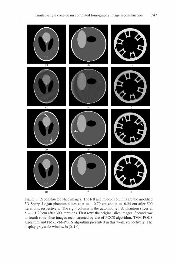
Figure 3. Reconstructed slice images. The left and middle columns are the modified3D Shepp–Logan phantom slices at z D �0:70 cm and x D 0:24 cm after 500iterations, respectively. The right column is the automobile hub phantom slices atz D �1:29 cm after 300 iterations. First row: the original slice images. Second rowto fourth row: slice images reconstructed by use of POCS algorithm, TVM-POCSalgorithm and PM-TVM-POCS algorithm presented in this work, respectively. Thedisplay grayscale window is Œ0; 1:0�.


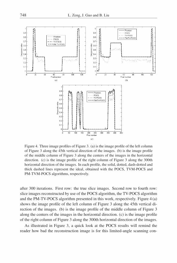
Figure 4. Three image profiles of Figure 3. (a) is the image profile of the left columnof Figure 3 along the 45th vertical direction of the images. (b) is the image profileof the middle column of Figure 3 along the centers of the images in the horizontaldirection. (c) is the image profile of the right column of Figure 3 along the 300thhorizontal direction of the images. In each profile, the solid, dotted, dash-dotted andthick dashed lines represent the ideal, obtained with the POCS, TVM-POCS andPM-TVM-POCS algorithms, respectively.

after 300 iterations. First row: the true slice images. Second row to fourth row:slice images reconstructed by use of the POCS algorithm, the TV-POCS algorithmand the PM-TV-POCS algorithm presented in this work, respectively. Figure 4 (a)shows the image profile of the left column of Figure 3 along the 45th vertical di-rection of the images. (b) is the image profile of the middle column of Figure 3along the centers of the images in the horizontal direction. (c) is the image profileof the right column of Figure 3 along the 300th horizontal direction of the images.

As illustrated in Figure 3, a quick look at the POCS results will remind thereader how bad the reconstruction image is for this limited-angle scanning con-


figuration. Furthermore, the reconstruction images of the TVM-POCS algorithmhave artifacts with gradual change gray regions which are pointed out by the arrow-head (the third row of Figure 3). By introducing the piecewise-constant constrainas a penalty term into TVM-POCS algorithm iterative steps, the PM-TVM-POCSalgorithm can generate better reconstruction images for the limited-angle circularcone-beam CT obviously, and the results of the PM-TVM-POCS iterative recon-struction algorithm are visually indistinguishable from the true image. From theprofiles of Figure 4 we can draw the same conclusion that the reconstruction imageof the PM-TVM-POCS algorithm is more approximate to the true image.

To verify the presented algorithm’s advantage and stability for noise, we havealso applied the above algorithms to the noisy data by adding Poisson noise basedon an emission of 106 photons to the 3D Shepp–Logan phantom projection data. Inthis noisy simulation experiment, we have the maximal iterative number Ncount D

600, the TVM-POCS iterative number for obtaining the initialization reconstruc-tion image NTVM-POCS D 500, the TV gradient descent algorithm step size a D0:2, the iterative number Ngrad D 20, the interval of piecewise-constant modifi-cation iterative number Npc D 20, the maximal outflow (reduction) gray of eachvoxel T D 20, cmin D 0:025 and cmax D 20. Some typical reconstructed slices areshown in Figure 5. Figure 6 shows the image profiles of Figure 5.

The reconstructed slice images of the modified 3D Shepp–Logan phantom fromnoisy projection data after 600 iterations are shown in Figure 5. The top andbottom row are the slices at z D �0:70 cm and x D 0:24 cm, respectively. Firstcolumn to third column: slice images reconstructed by use of the POCS algorithm,the TV-POCS algorithm and the PM-TV-POCS algorithm presented in this work,respectively. In Figure 6 (a) is the image profile of the top row of Figure 5 alongthe 45th vertical direction of the images. (b) is the image profile of the bottom rowof Figure 5 along the centers of the images in the horizontal direction.

As shown in Figure 5, a quick glance at the POCS results will remind the readerhow bad the reconstruction image is for this limited-angle scanning configuration,and that the noise has great effect on POCS algorithm reconstruction. But thenoise has little effect on TVM-POCS reconstruction, because the TVM-POCS al-gorithm can smooth out noise. However, like the noiseless case, the reconstructionimages of the TVM-POCS algorithm have artifacts with gradual change gray re-gions. By introducing the piecewise-constant constrain as a penalty term into theTVM-POCS algorithm, the PM-TVM-POCS algorithm also keeps the ability tosmooth out noise, and the results are visually indistinguishable from the true im-age. The profiles of Figure 6 also demonstrate that the reconstruction image of thePM-TVM-POCS algorithm is more approximate to the true image and the noisehas little effect on PM-TVM-POCS reconstruction.


Figure 5. Reconstructed slice images of the modified 3D Shepp–Logan phantomfrom noisy projection data after 600 iterations. The top and bottom row are the slicesat z D �0:70 cm and x D 0:24 cm, respectively. First column to third column: sliceimages reconstructed by use of POCS algorithm, TVM-POCS algorithm and PM-TVM-POCS algorithm presented in this work, respectively. The display grayscalewindow is Œ0; 1:0�.

For quantitative analysis to compare the reconstruction results, the quantitativeanalyses conducted in terms of mean square error (MSE) [5] is presented in Ta-ble 3. The MSE is calculated by

MSE D1

N

NXiD1

�f .Eri / � Of .Eri /

�2;

where f .Eri / and Of .Eri / denote the ideal vale and reconstructed value, respectively.N indicates the total number of the set points.

From Table 3 we can see that the MSE of the image reconstructed by the PM-TVM-POCS algorithm is much less than those of the POCS and TVM-POCS al-gorithms. Moreover, the noise has little effect on PM-TVM-POCS reconstruction.

It should be pointed out that the studies here are designed to illustrate the perfor-mance of the PM-TVM-POCS algorithm, and the values of the algorithm param-eters may not be optimal. The optimal values usually depend on the underlyingimage function.


Figure 6. Two image profiles of Figure 5. (a) is the image profile of the top row ofFigure 5 along the 45th vertical direction of the images. (b) is the image profile ofthe bottom row of Figure 5 along the centers of the images in the horizontal direc-tion. In each profile, the solid, dotted, dash-dotted and thick dashed lines representthe ideal, obtained with the POCS, TVM-POCS and PM-TVM-POCS algorithms,respectively.

POCS TVM-POCS PM-TVM-POCS

Shepp–Logan phantom 1.06 e-2 1.48 e-3 3.57 e-4Automobile hub 9.00 e-3 2.80 e-3 7.00 e-4Noisy data 1.31 e-2 2.81 e-3 4.83 e-4

Table 3. MSE of the reconstructed images.

5 Conclusion

In this paper, for the problem of reconstructed images having artifacts with grad-ual change gray from limited-angle cone-beam scanning data by the TVM-POCSalgorithm, on the basis of the TVM-POCS algorithm, we introduce a piecewise-constant constrain as a penalty term into TVM-POCS iterative to develop an im-proved iterative reconstruction algorithm for limited-angle circular cone-beam CT,which is referred to as the PM-TVM-POCS algorithm. Simulation experimentalresults show that the presented algorithm can solve the problem of insufficient re-construction region by the TVM-POCS and improve the quality of reconstructedimages significantly. In addition, it is robust to noise. Although in some sense,the piecewise-constant modification algorithm is a heuristic approach, it is simpleand effective. Because the running time of piecewise-constant modification is far


less than the iterative running time of the TVM-POCS algorithm, the running timeof the PM-TVM-POCS algorithm is almost equivalent to that of the TVM-POCSalgorithm. Like other iterative algorithms, this algorithm is time-consuming andaccelerating is our next task. Although only simulation experiments are presentedin the experiment part, the TVM algorithm has been used to realistic image recon-structions and gets good results [22]. Of course, if the gray of the reconstructedimage itself is gradually changed, this algorithm will be restricted. It is clear thatthis algorithm can be easily applied to other CT configurations with small modifi-cations.

Bibliography

[1] D. S. Anikonov, External sources of resonance type in X-ray tomography, J. InverseIll-Posed Probl. 17 (2009), 311–320.

[2] J. M. Boone, N. Shah and T. R. Nelson, A comprehensive analysis of DgN(CT)coefficients for pendant-geometry cone-beam breast computed tomography, Med.Phys. 31 (2004), 226–235.

[3] E. J. Candes, J. Romberg and T. Tao, Robust uncertainty principles: Exact signal re-construction from highly incomplete frequency information, IEEE Trans. Inf. Theory52 (2006), 489–509.

[4] E. J. Candes, J. Romberg and T. Tao, Stable signal recovery from incomplete andinaccurate measurements, Commun. Pure Appl. Math. 59 (2006), 1207–1223.

[5] K. Chidlowy and T. Möller, Rapid emission tomography reconstruction, in: Proceed-ings of the 3rd International Workshop on Volume Graphics, Tokyo (2003), 15–26.

[6] P. L. Combettes, The foundations of set theoretic estimation, Proc. IEEE 81 (1993),182–208.

[7] M. J. Daly, J. H. Siewerdsen, D. J. Moseley, D. A. Jaffray and J. C. Irish, Intraopera-tive cone-beam CT for guidance of head and neck surgery: Assessment of dose andimage quality using a C-arm prototype, Med. Phys. 33 (2006), 3767–3780.

[8] A. H. Delaney and Y. Bresler, Globally convergent edge-preserving regularized re-construction: An application to limited-angle tomography, IEEE Trans. Image Proc.7 (1998), 204–221.

[9] D. L. Donoho, Compressed sensing, IEEE Trans. Inf. Theory 52 (2006), 1289–1306.

[10] A. B. Gonzalez et al., Projected cancer risks from computed tomographic scans per-formed in the United States in 2007, Arch. Intern. Med. 169 (2009), 2071–2077.

[11] C. G. Ji, Accurrate 3D data stitching in circular cone-beam micro-CT, J. X-Ray Sci.Technol. 18 (2010), 99–110.


[12] C. Kaka and M. Slaney, Principles of Computerized Tomographic Imaging, IEEEPress, New York, 1999.

[13] D. Letourneau et al., Cone-beam-CT guided radiation therapy: technical implemen-tation, Radiat. Oncol. 75 (2005), 279–286.

[14] M. Persson, D. Bone and H. Elmqvist, Three-dimensional total variation norm forSPET reconstruction, Nucl. Instrum. Methods Phys. Res. 471 (2001), 98–102.

[15] S. Pursiainen, Coarse-to-fine reconstruction in linear inverse problems with applica-tion to limited-angle computerized tomography, J. Inverse Ill-Posed Probl. 8 (2008),873–886.

[16] L. I. Rudin, S. Osher and E. Fatemi, Nonlinear total variation based noise removalalgorithms, Physica D 60 (1992), 259–268.

[17] E. Y. Sidky, C. M. Kao and X. C. Pan, Accurate image reconstruction from few-viewsand limited-angle data in divergent-beam CT, J. X-Ray Sci. Technol. 14 (2006), 119–139.

[18] E. Y. Sidky and X. C. Pan, Image reconstruction in circular cone-beam computed to-mography by constrained, total-variation minimization, Phys. Med. Biol. 53 (2008),4777–4807.

[19] R. Smith-Bindman et al., Radiation dose associated with common computed tomog-raphy examinations and the associated lifetime attributable risk of cancer, Arch. In-tern. Med. 169 (2009), 2078–2086.

[20] G. Wang, Y. Li and M. Jiang, Uniqueness theorems in bioluminescence tomography,Med. Phys. 31 (2004), 2289–2299.

[21] Y. Xu and O. Tischenko, OPED reconstruction algorithm for limited angle problem,J. Inverse Ill-Posed Probl. 17 (2009), 795–813.

[22] H. Y. Yu and G. Wang, Compressed sensing based interior tomography, Phys. Med.Biol. 54 (2009), 2791–2805.

[23] K. Zeng et al., An in vitro evaluation of cone-beam breast CT methods, J. X-Ray Sci.Technol. 16 (2008), 171–187.


Received May 30, 2011.

Author information

Li Zeng, ICT Research Center, Key Laboratory of Optoelectronic Technology andSystem of the Education Ministry of China, Chongqing University, Chongqing, 400044;and College of Mathematics and Statistics, Chongqing University, Chongqing, 401331,P. R. China.E-mail: [email protected]

Jiqiang Guo, ICT Research Center, Key Laboratory of Optoelectronic Technology andSystem of the Education Ministry of China, Chongqing University, Chongqing, 400044;and College of Optoelectronic Engineering, Chongqing University, Chongqing, 400044,P. R. China.E-mail: [email protected]

Baodong Liu, School of Electronic Engineering, Tianjin University of Technology andEducation, Tianjin, 300222, P. R. China.

mailto:[email protected]

mailto:[email protected]

Copyright of Journal of Inverse & Ill-Posed Problems is the property of De Gruyter and itscontent may not be copied or emailed to multiple sites or posted to a listserv without thecopyright holder's express written permission. However, users may print, download, or emailarticles for individual use.

本文献由“学霸图书馆-文献云下载”收集自网络，仅供学习交流使用。

学霸图书馆（www.xuebalib.com）是一个“整合众多图书馆数据库资源，

提供一站式文献检索和下载服务”的24 小时在线不限IP

图书馆。

图书馆致力于便利、促进学习与科研，提供最强文献下载服务。

图书馆导航：

图书馆首页文献云下载图书馆入口外文数据库大全疑难文献辅助工具

http://www.xuebalib.com/cloud/

http://www.xuebalib.com/

http://www.xuebalib.com/cloud/


http://www.xuebalib.com/vip.html

http://www.xuebalib.com/db.php

http://www.xuebalib.com/zixun/2014-08-15/44.html


limited-angle cone-beam computed tomography image

Documents