linear control systems - montefiore instituteguilldrion/files/syst0003-2017-18-tp4.pdf · linear...

LinearControlSystemsProjectsession4:Designinfrequencydomain

Kathleen [email protected]

1

20th October 2017

Content

2

1. Time domain >< Frequency domain

2. Frequency domain analysisv Procedurev Transfer functionv Design considerationv Simulations specifications

3. Loop Shapingv Reminderv Compensatorv Low pass filterv PI controllerv Anti windup

4. Final controller

5. Feedforward6. Noise7. Gang of four8. Delays

Time domain >< Frequency domain

3

Conclusion of the time domain

0 0.2 0.4 0.6 0.8 1 1.2 1.4 1.6 1.8 2

Time(s)

0.392

0.394

0.396

0.398

0.4

0.402

0.404

0.406

0.408

Distance(m)

0 0.2 0.4 0.6 0.8 1 1.2 1.4 1.6 1.8 2

Time(s)

-4

-3

-2

-1

0

1

2

3

4

Acceleration(m/s2 )

Relative distance Acceleration

▷ Static error when v=cst▷ Noise rejection: quite good▷ Reference tracking: quite good▷ Delays: could be improved

Move to frequency domain

Content

4




4. Final controller


Frequency domain analysis

5

Procedure▷ Step 1: Determining transfer function▷ Step 2: Updating the constraints compared to the time domain,

the design considerations and simulations specifications▷ Step 3: Performing the loop shaping▷ Step 4: Optimising the final controller


6

Transfer function H(s)=C (sI-A)-1 B + D

H1(s)=

H2(s)=1

1/ms2 1/m

s2P(s)=Only the controllable input

Mag

nitu

de (d

B)Ph

ase

(deg

)

Frequency (rad/s)

Bode plot of P(s)


7

▷ Maximum real acceleration: 4 m/s2

▷ Maximum derivation: better then in time domain

▷ Choice of the frequency cross-over: /!\reminder

- the amplitudes at frequencies lower than fco are amplified.- the amplitudes at greater frequencies are attenuated.- the value of fco is fixed by taking into account the limitations of the system.

- At which frequency does the system work ? A miniaturised car can follow maximum two oscillations of the vehicle in front during on second: fwork=2Hz.

- What could be a reasonable choice for the cross-over frequency ? fco =4Hz

Design considerations/!\ Key steps


8

▷ Delays: For example: constraint from the microcontroller or from the sensor.For the TJA: fsensor= 20Hz ó one information each 50ms.

▷ Measurement noise: the sensor is affected by noise.

▷ Load disturbance: For the TJA, it corresponds to the displacement of the car in front?a very good load disturbance reaction is required.

Design considerations/!\ Key steps


9

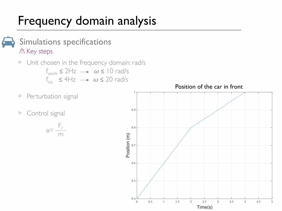
▷ Unit chosen in the frequency domain: rad/sfwork ≤ 2Hz 𝜔 ≤ 10 rad/sfco. ≤ 4Hz 𝜔 ≤ 20 rad/s

▷ Perturbation signal

▷ Control signal

a=

Simulations specifications/!\ Key steps

Time(s)

Posi

tion

(m)

Position of the car in front

Frm

Content

10




4. Final controller


Loop Shaping

Reminder: nyquist approach

11

Based on the Nyquist stability theorem, tools are developed to work in the frequency domain and design a good controller. (more explanations chapter 9 of the book)

Loop Shaping

Reminder: nyquist approach

12

“One of the powerful concepts embedded in the Nyquist’s approach to stability analysis isthat it allows us to study the stability of the feedback system by looking at the propertiesof the loop transfer function.The advantage is to see how the controller should be chosento obtain desired loop transfer function.” (chap.9 p.261)

Stability margins describes how stable the system is and its robustness to perturbations.

Loop Shaping

Reminder: L(s)

13

Loop function: L(s)

L(s)=P(s)C(s)

- Trial-and-error procedure

- Add gains, poles and zeros until the desired shape is obtained.(more explanations chapter 11 paragraph 4 of the book)

- Modification of C(s) and in the feedback loop changes the shape of L(s). This modification can be read on the Nyquist Plot.

Loop Shaping

14

Reminder

Adding a new block in the feedback loop can be analysed in your Nyquist plot.For example, here we add delays in the loop.

Loop Shaping

Reminder

Real Axis

Imag

inar

y Ax

is

Nyquist plot for different delays

Instabilities are detected. In this example, delays greater than 0.06s are not possible.

Loop Shaping

Block diagram

▹ Add components in your controller to shape your loop transfer function with your desired specifications.

16

40cm

▹ Procedure to study the impact of each block on the controller- Describe the usefulness of the component- Study the parameters- See the modification in the frequency domain (analyse L(s))- Check your criteria on simulations in the time domain = Check if the reference tracking is improved and if your controllable input is feasible.

Loop Shaping

Compensator

17

▷ UsefulnessTwo types of compensators (ex: page 328)

Bode plot of a lead compensator Bode plot of a lag compensator

1st idea: use a lag to increase the gain at LF brings instabilities and a very low phase margin2nd idea: use a lead to increase the phase margin

Loop Shaping

Compensator

18

▷ Parameters- equation of the lead compensator:- parameters: GLo ,wz and wp- how determine them ?

I used a procedure* which provides their values for a given cross over frequency fcoand a given phase margin Pm. There are different ways to fixe the values depending on your control problem.

*seen in Power Electronics with M. Frebel. The reference book is Fundamentals of Power Electronics, Robert W. Erickson

Loop Shaping

Compensator

19

▷ Simulation in frequency domain Useful to see how your L(s) evolvesM

agni

tude

(dB)

Phas

e (d

eg)

Pm=60°Pm=70°Pm=80°

Frequency (rad/s)

Bode plot of L(s) for different phase margin

Loop Shaping

Compensator

20

▷ Simulations in time domain

Time (s)

Dis

tanc

e (m

)

Pm=60°Pm=70°Pm=80°

Relative distance for different values of phase margin

Loop Shaping

Compensator

21


Time (s)

Acce

lera

tion

(m/s

2 )

Pm=60°Pm=70°Pm=80°

Acceleration for different values of phase margin

Loop Shaping

Compensator

22

▷ ResultTrade-off between delays and fast response

Chosen values for the parameters: fixed for Pm=70°(wz , wp and Glo are computed following the procedure described on slide 13)

Loop Shaping

Low pass filter

23

▷ UsefulnessReduce the noise which could affect the system.How? By decreasing the gain at high frequencies.

▷ Parametersequation of a low pass filter :

parameters: cut-off frequency=whf

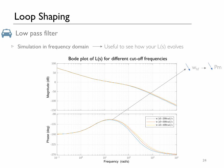
Loop Shaping

Low pass filter

24

▷ Simulation in frequency domain Useful to see how your L(s) evolvesM

agni

tude

(dB)

Phas

e (d

eg)

Frequency (rad/s)

Bode plot of L(s) for different cut-off frequencies

whf Pm

Loop Shaping

Low pass filter

25


Time (s)

Dis

tanc

e (m

)

w_hf=200rad/sw_hf=300rad/sw_hf=400rad/s

Relative distance for different cut-off frequencies

Loop Shaping

Low pass filter

26


Time (s)

Acce

lera

tion

(m/s

2 )

w_hf=200rad/sw_hf=300rad/sw_hf=400rad/s

Acceleration for different cut-off frequencies

Loop Shaping

Low pass filter

27

▷ ResultTrade-off between the phase margin and the noise rejection

Chosen value for the parameter: whf =300rad/s

Loop Shaping

PI controller

28

▷ Usefulnesscommon block used in Loop Shapingequation of a PI controller :

▷ Parameters- kp moves the magnitude of the frequency response of the system up or down and

hence it is used to set the cross-over frequency.But in the final controller, the overall gain is added taking into account GLo GHFo and kp.

kp=1 because the overall gain will be used to set the amplitude of L(s) equal to 0dB at wco.

- ki forces the open loop system to be nearly infinite at very low frequencies, i.e. at steadystate. It is this effect that forces the closed-loop system to have a zero steady state error.

BUT for the TJA with P(s)= , an integrator is already present and provides a very highamplitude at LF. By consequent, it removes the static error which existed in the time domain.

Let’s study ki to see if it can improve the controller.

1/ms2

Loop Shaping

PI controller

29

▷ Simulation in frequency domain Useful to see how your L(s) evolves

Bode plot of L(s) for different values of ki

Loop Shaping

PI controller

30


Relative distance for different values of ki

44

4

4

4

4

4

3

3

3

Loop Shaping

PI controller

31


Acceleration for different values of ki

Loop Shaping

PI controller

32

▷ ResultUseless block in the controller and lead to undesired behavior

Loop Shaping

Anti windup

▷ Integrator Windup: described in chapter 10 paragraph 4▷ Purpose: integral terms accumulates a significant error during the rise of this

error. This leads to the saturation of the integral term. The solution is to imposean upper limit and the integral term can not take values above this limit.

▷ For the TJA: SIMULINK adds automatically the anti windup property for the integral term

33

Content

34




4. Final controller


Final controller

35

Summary

Final controller

Final Loop transfer function

Loop transfer function for the entire closed loop system

Final controller

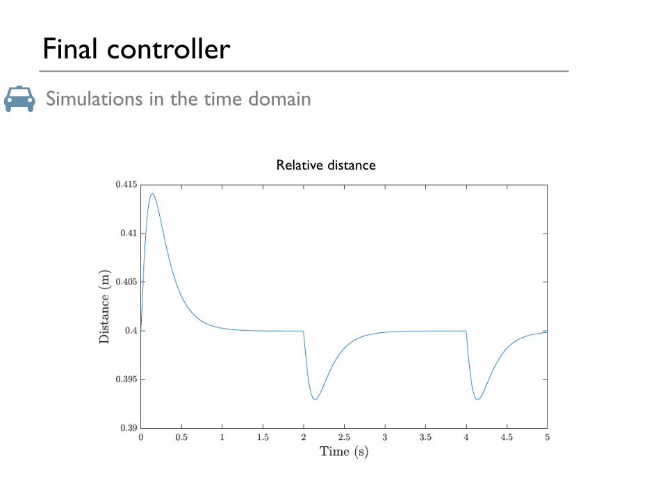
Simulations in the time domain

Relative distance

Final controller

Simulations in the time domain

Acceleration

Final controller

39

see the phase marginThe angle between the horizontal line(180°) andthe intersection of the plot and the unitary circle

Nyquist plot

Final controller

40

Nyquist plot

Amplitude is very big for small frequencies.(due to the shape of P(s))

It favors a good reference tracking.

Amplitude is decreasing for high frequencies.It shows the noise rejection.

Final controller

Analysis Check your design considerations

41

Content

42




4. Final controller


Feedforward

Reminder

▷ Technique that is complementary to the feedback.▷ Used to improve the response to the reference signals and to reduce the effect of

a measurable disturbances.▷ Controller with two degrees of freedom (feedback and feedforward)▷ More explanations chapter 11 paragraph 2

Comparison between feedback and feedforward

Feedback takes into corrective actions to counteract the measured error after a perturbation has affected the system.>< Feedforward allows to measure a disturbance before it enters the system. It is possible to take a corrective action before the disturbance has influenced the system.

43

Feedforward

For the TJADiscussion for the two inputs

▷ Input 2 = Load disturbanceAdding a feedforward control for this input = creating a direct communicationbetween the two vehicles.

▷ Input 1= Resulting force applied on car2Adding a feedforward control for this input = obtaining information related tothe road; slope, friction forces due to the coating, weather conditions, …

44

Content

45




4. Final controller


Noise

46

SimulationsThe position of the two vehicles are given by two sensors. If these values are stronglydisturbed, the relative distance is not enough accurate and the controller tries to adjustthe power injected to the motor based on wrong values. So, the tracking is not correct.

Block diagram on SIMULINK

Noise

Simulations in time domain

Time (s)

Dis

tanc

e (m

)Related distance affected by noise

Noise


Related distance affected by noise

Time (s)

Acce

lera

tion

(m/s

2 )Acceleration affected by noise

Content

49




4. Final controller


Gang of four

50

Sensitivity function

This function provides information of the noise to the output of the system ( Gyn ).

Bode plot of the sensitivity function SHF: amplitude ~0dBOutput is affected by the noise

Peak stability margin

Gang of four

51

Bode plot of the complementary sensitivity function TLF: amplitude ~0dBLF corresponds to the range of frequencies of the load disturbance.Good tracking of the reference andGood reaction to the load disturbance

HF: rejection

Complementary sensitivity function T=

This function shows the influence of the reference on the output of the system ( Gyr )and also the influence of the load disturbance on the output of the controller (Gud ).

Content

52




4. Final controller


Delays

53

Representation

Expression of a delay:

Block diagram on SIMULINK:

Delays

Simulations in frequency domain

Real Axis

Imag

inar

y Ax

is

Real Axis

Imag

inar

y Ax

is

Real Axis

Imag

inar

y Ax

is

Nyquist plot for different delays

Delays


Real Axis

Imag

inar

y Ax

is

Real Axis

Imag

inar

y Ax

is

Time (s)

Dis

tanc

e (m

)

t_d=0.03st_d=0.05st_d=0.07s

Relative distance for different delays

Delays


Real Axis

Imag

inar

y Ax

is

Real Axis

Imag

inar

y Ax

is

Time (s)

Acce

lera

tion

(m/s

2 )

t_d=0.03st_d=0.05st_d=0.07s

Acceleration for different delays

Delays

Results

▹ fsensor=20Hz which corresponds to a delay equals to 50ms.

▹ Simulations: small oscillationsfor better results, it should be interesting to use a faster sensor.

linear control systems - montefiore instituteguilldrion/files/syst0003-2017-18-tp4.pdf · linear...

Documents