linear regression model -...
TRANSCRIPT
04/10/15
1
Linear regression model
Models in general
04/10/15
2
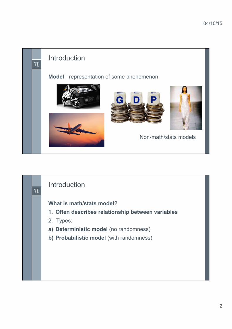
Introduction Model - representation of some phenomenon
Non-math/stats models
Introduction What is math/stats model? 1. Often describes relationship between variables 2. Types: a) Deterministic model (no randomness) b) Probabilistic model (with randomness)
04/10/15
3
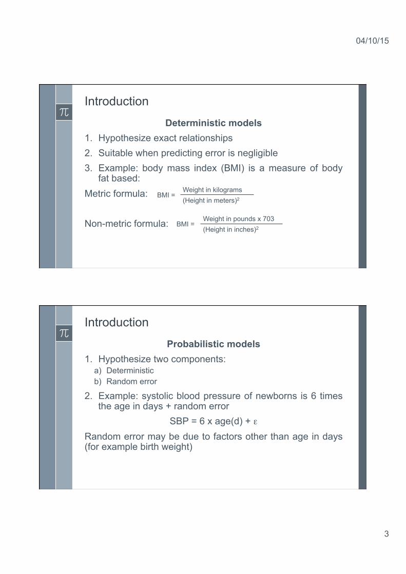
Introduction
Deterministic models 1. Hypothesize exact relationships 2. Suitable when predicting error is negligible 3. Example: body mass index (BMI) is a measure of body
fat based: Metric formula: Non-metric formula:
BMI = Weight in kilograms (Height in meters)2
BMI = Weight in pounds x 703 (Height in inches)2
Introduction
Probabilistic models 1. Hypothesize two components:
a) Deterministic b) Random error
2. Example: systolic blood pressure of newborns is 6 times the age in days + random error
SBP = 6 x age(d) + ε Random error may be due to factors other than age in days (for example birth weight)
04/10/15
4
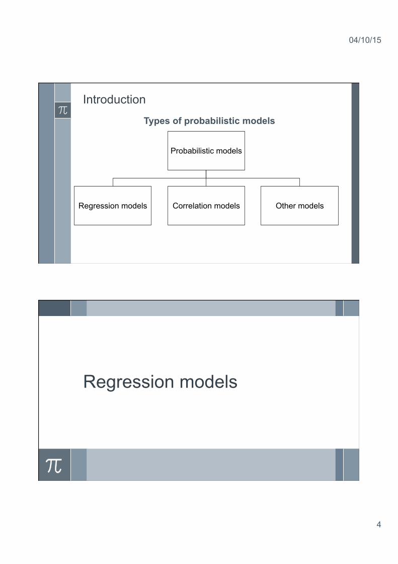
Introduction
Types of probabilistic models
Probabilistic models
Regression models Correlation models Other models
Regression models
04/10/15
5
Introduction Regression analysis is perhaps the most widely used method for the analysis of dependence – that is, for examining the relationship between a set of independent variables (X’s) and a single dependent variable (Y). Regression (in general) is a linear combination of independent variables that corresponds as closely as possible to the dependent variable. Regression models are used for purposes of description, inference and prediction.
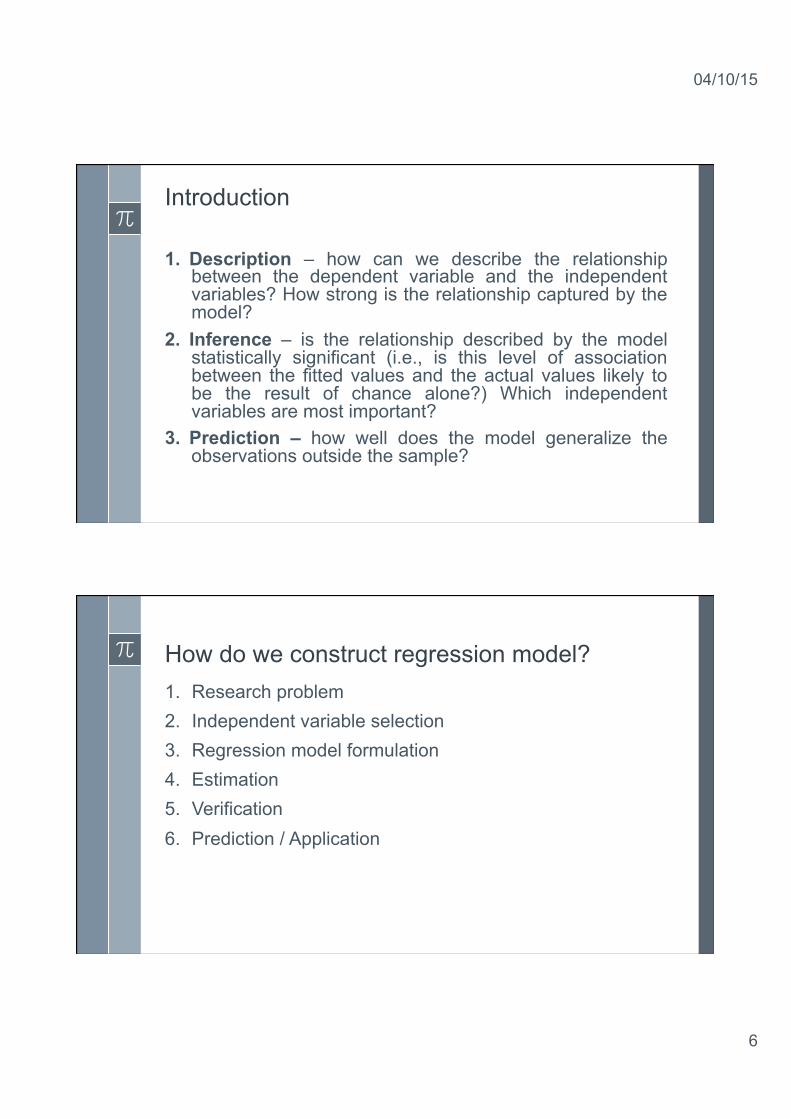
Regression model vs mathematic function (model)
Some linear mathematical functions Linear regression model
04/10/15
6
Introduction 1. Description – how can we describe the relationship
between the dependent variable and the independent variables? How strong is the relationship captured by the model?
2. Inference – is the relationship described by the model statistically significant (i.e., is this level of association between the fitted values and the actual values likely to be the result of chance alone?) Which independent variables are most important?
3. Prediction – how well does the model generalize the observations outside the sample?
How do we construct regression model? 1. Research problem 2. Independent variable selection 3. Regression model formulation 4. Estimation 5. Verification 6. Prediction / Application
04/10/15
7
Model specification Is based on theory: 1. Theory of field (economic, epidemiology, etc.) 2. Mathematical theory 3. Previous research 4. „Common sense”
Variable selection for the model We have to choose independent variables for our model. In general two approaches are proposed: 1. Substantive approach – we choose variables according
to some theory, experts, former regression models, etc. 2. Substantive – formal approach – first we use
substantive approach to build a list of possible variables, then we use some formal approaches to select best of them
04/10/15
8
Formal approaches for variable selection Some (it’s not a complete list) of the formal approaches: 1. Coefficient of variation:
We calculate this coefficient for each variable. Then some critical value V* is set (usually V* = 0.1). If the variable j has its coefficient grater than V* it can be in the model, otherwise it should not be considered in the model
j
jj xs
V =
Formal approaches for variable selection 2. Hellwig’s method Three steps: a) Number of combinations: 2m-1
b) Individual capacity of every independent variable in the combination:
c) Integral capacity of information for every combination:
∑∈
=
kIiij
jkj r
rh
20
∑= kjk hH
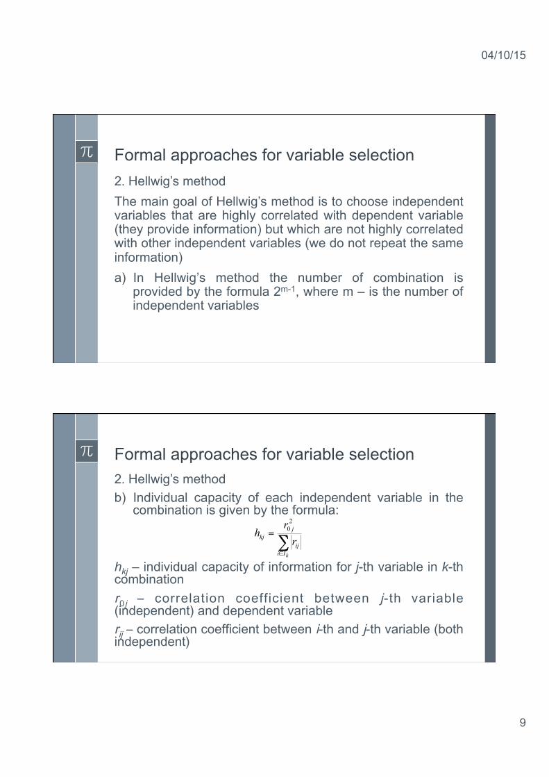
04/10/15
9
Formal approaches for variable selection 2. Hellwig’s method The main goal of Hellwig’s method is to choose independent variables that are highly correlated with dependent variable (they provide information) but which are not highly correlated with other independent variables (we do not repeat the same information) a) In Hellwig’s method the number of combination is
provided by the formula 2m-1, where m – is the number of independent variables
Formal approaches for variable selection 2. Hellwig’s method b) Individual capacity of each independent variable in the
combination is given by the formula:
hkj – individual capacity of information for j-th variable in k-th combination r0 j – correlation coefficient between j-th variable (independent) and dependent variable rij – correlation coefficient between i-th and j-th variable (both independent)
∑∈
=
kIiij
jkj r
rh
20
04/10/15
10
Formal approaches for variable selection 2. Hellwig’s method c) Integral capacity of information for every combination The next step is to calculate Hk – integral capacity of information for each combination as the sum of individual capacities of information within each combination: We choose the variables from the combination with the highest integral capacity of information
∑= kjk hH
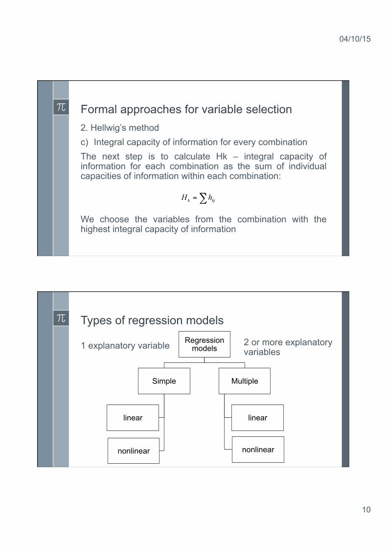
Types of regression models Regression
models
Simple
linear
nonlinear
Multiple
linear
nonlinear
2 or more explanatory variables
1 explanatory variable
04/10/15
11
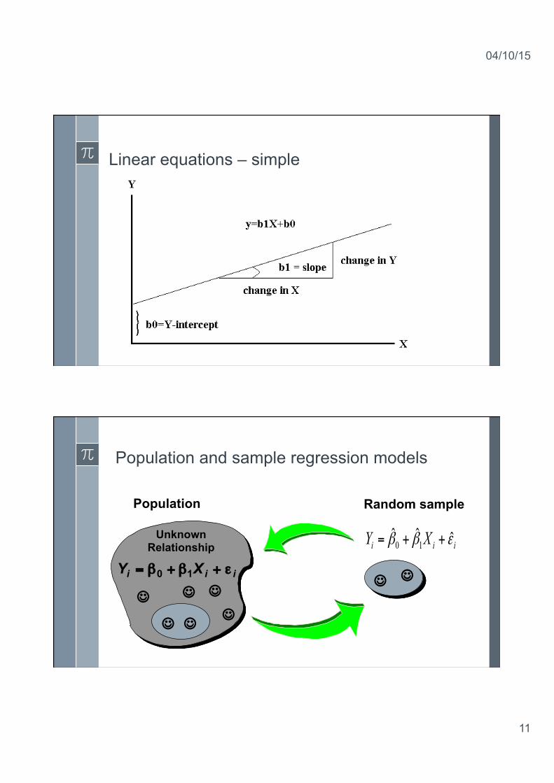
Linear equations – simple
Population and sample regression models
Unknown Relationship
Y Xi i i= + +β β ε0 1
J J
J J J J
Population Random sample
J J
iii XY εββ ˆˆˆ10 ++=
04/10/15
12
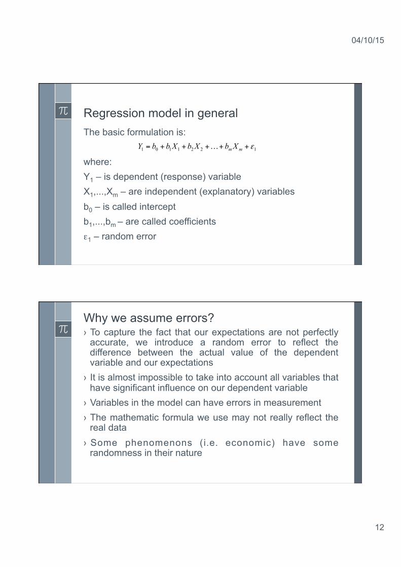
Regression model in general The basic formulation is: where: Y1 – is dependent (response) variable X1,...,Xm – are independent (explanatory) variables b0 – is called intercept b1,...,bm – are called coefficients ε1 – random error
1221101 ε+++++= mmXbXbXbbY …
Why we assume errors? › To capture the fact that our expectations are not perfectly
accurate, we introduce a random error to reflect the difference between the actual value of the dependent variable and our expectations
› It is almost impossible to take into account all variables that have significant influence on our dependent variable
› Variables in the model can have errors in measurement › The mathematic formula we use may not really reflect the
real data › Some phenomenons (i.e. economic) have some
randomness in their nature
04/10/15
13
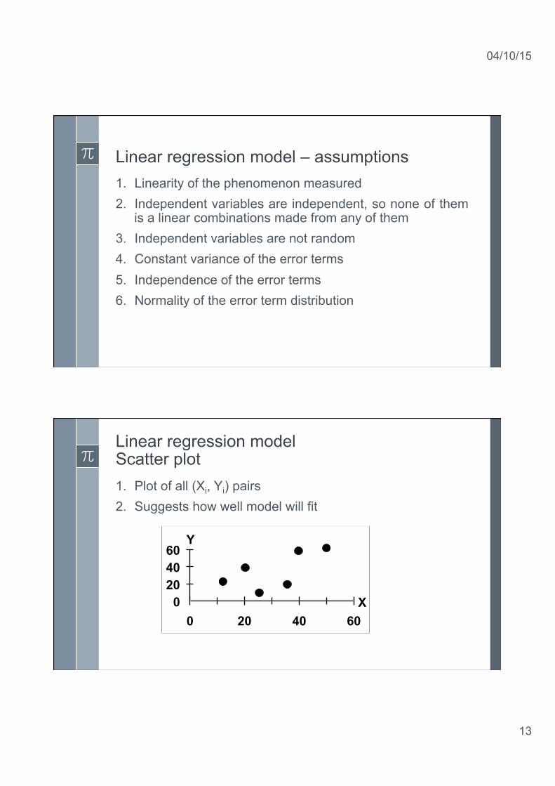
Linear regression model – assumptions 1. Linearity of the phenomenon measured 2. Independent variables are independent, so none of them
is a linear combinations made from any of them 3. Independent variables are not random 4. Constant variance of the error terms 5. Independence of the error terms 6. Normality of the error term distribution
Linear regression model Scatter plot 1. Plot of all (Xi, Yi) pairs 2. Suggests how well model will fit
0 20 40 60
0 20 40 60 X
Y
04/10/15
14
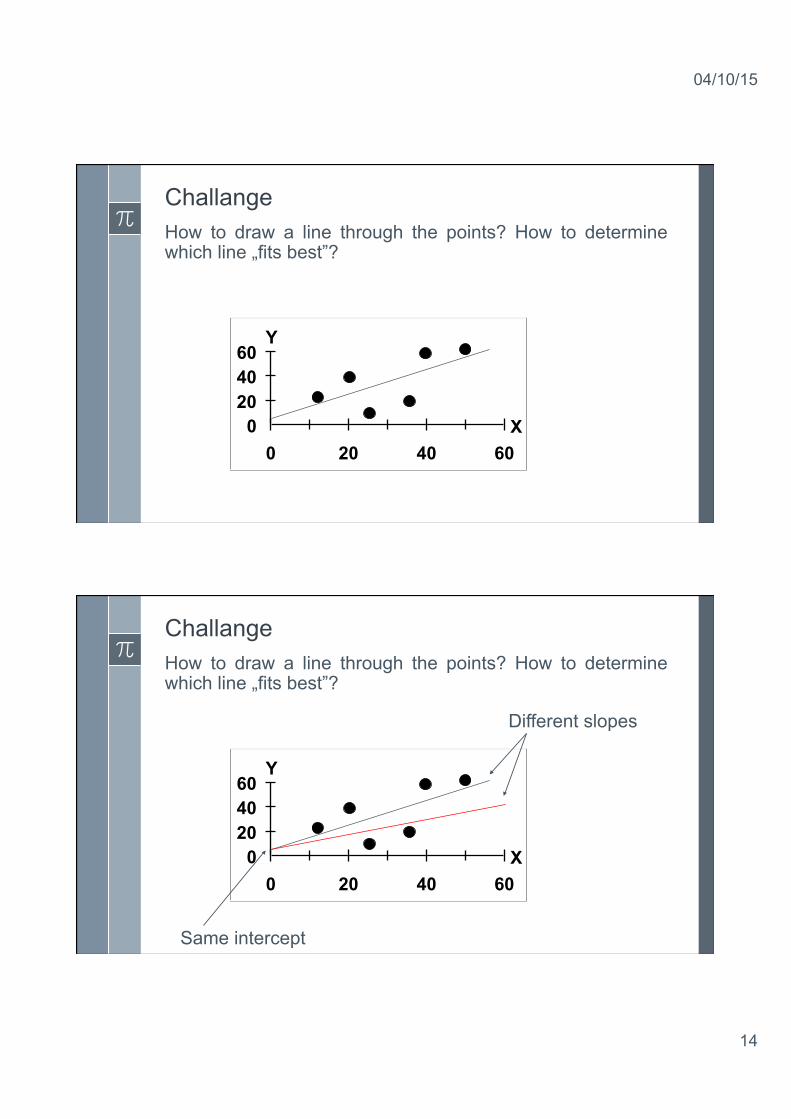
Challange How to draw a line through the points? How to determine which line „fits best”?
0 20 40 60
0 20 40 60 X
Y
Challange How to draw a line through the points? How to determine which line „fits best”?
0 20 40 60
0 20 40 60 X
Y
Different slopes
Same intercept
04/10/15
15
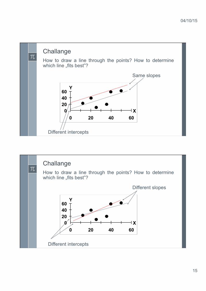
Challange How to draw a line through the points? How to determine which line „fits best”?
0 20 40 60
0 20 40 60 X
Y
Same slopes
Different intercepts
Challange How to draw a line through the points? How to determine which line „fits best”?
0 20 40 60
0 20 40 60 X
Y
Different slopes
Different intercepts
04/10/15
16
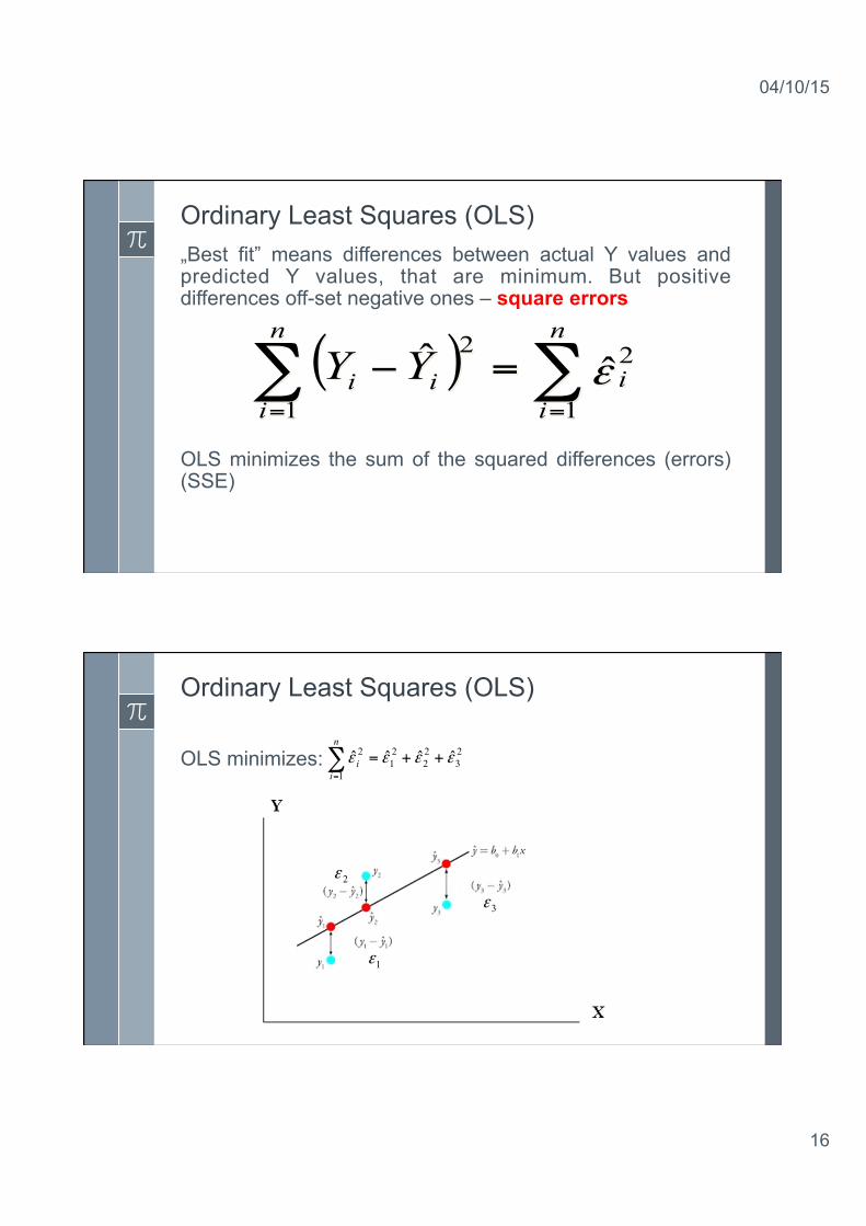
Ordinary Least Squares (OLS) „Best fit” means differences between actual Y values and predicted Y values, that are minimum. But positive differences off-set negative ones – square errors OLS minimizes the sum of the squared differences (errors) (SSE)
( ) ∑∑==
=−n
ii
n
iii YY
1
2
1
2ˆˆ ε
Ordinary Least Squares (OLS) OLS minimizes: 2
322
21
1
2 ˆˆˆ ˆ εεεε ++=∑=
n
ii
1ε
2ε
3ε
04/10/15
17
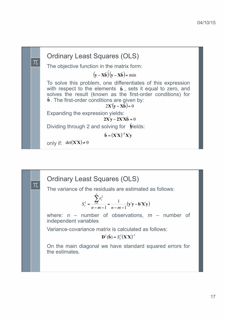
Ordinary Least Squares (OLS) The objective function in the matrix form: To solve this problem, one differentiates of this expression with respect to the elements , sets it equal to zero, and solves the result (known as the first-order conditions) for s . The first-order conditions are given by:
Expanding the expression yields:
Dividing through 2 and solving for yields: only if:
( ) ( ) minˆˆ =−ʹ′
− bXybXy
b
b
( ) 0ˆ2 =−ʹ′ bXyX
0ˆ =ʹ′−ʹ′ bXX2yX2b
( ) yXXXb 1 ʹ′ʹ′= −ˆ
( ) 0det ≠ʹ′XX
Ordinary Least Squares (OLS) The variance of the residuals are estimated as follows:
where: n – number of observations, m – number of independent variables Variance-covariance matrix is calculated as follows: On the main diagonal we have standard squared errors for the estimates.
( )yXbyy ʹ′ʹ′−ʹ′−−
=−−
=∑=
11
11
2
2
mnmn
eS
n
ii
e
( ) 122 )ˆ( −ʹ′= XXbD eS
04/10/15
18
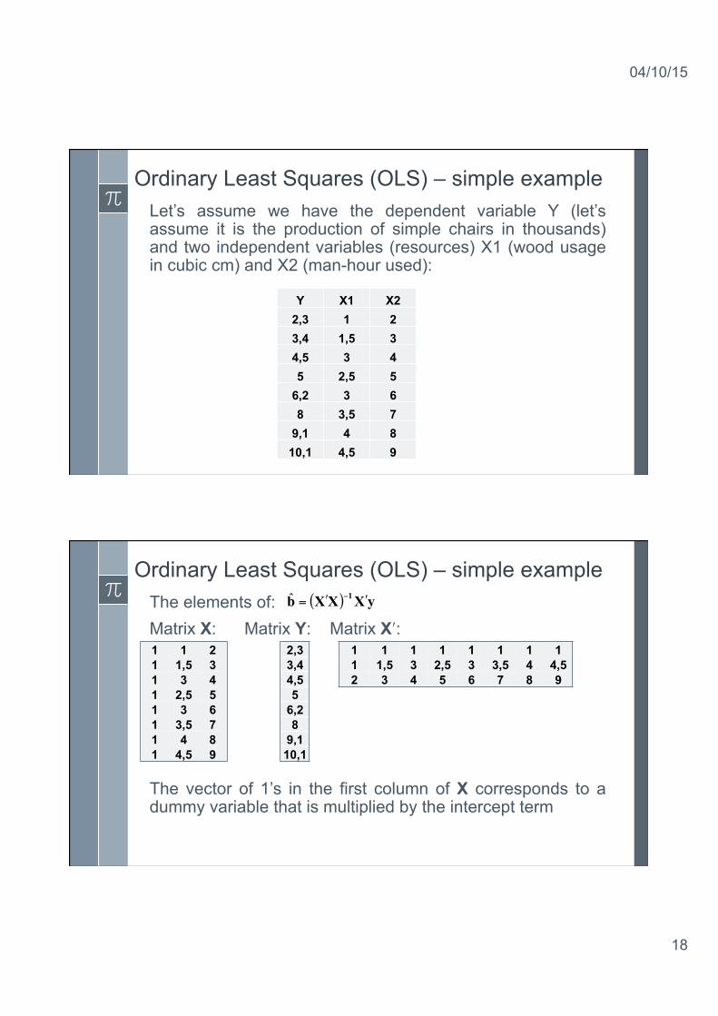
Ordinary Least Squares (OLS) – simple example Let’s assume we have the dependent variable Y (let’s assume it is the production of simple chairs in thousands) and two independent variables (resources) X1 (wood usage in cubic cm) and X2 (man-hour used):
Y X1 X2 2,3 1 2 3,4 1,5 3 4,5 3 4 5 2,5 5
6,2 3 6 8 3,5 7
9,1 4 8 10,1 4,5 9
Ordinary Least Squares (OLS) – simple example The elements of: Matrix X: Matrix Y: Matrix Xʹ′: The vector of 1’s in the first column of X corresponds to a dummy variable that is multiplied by the intercept term
( ) yXXXb 1 ʹ′ʹ′= −ˆ
1 1 2 1 1,5 3 1 3 4 1 2,5 5 1 3 6 1 3,5 7 1 4 8 1 4,5 9
2,3 3,4 4,5 5
6,2 8
9,1 10,1
1 1 1 1 1 1 1 1 1 1,5 3 2,5 3 3,5 4 4,5 2 3 4 5 6 7 8 9
04/10/15
19
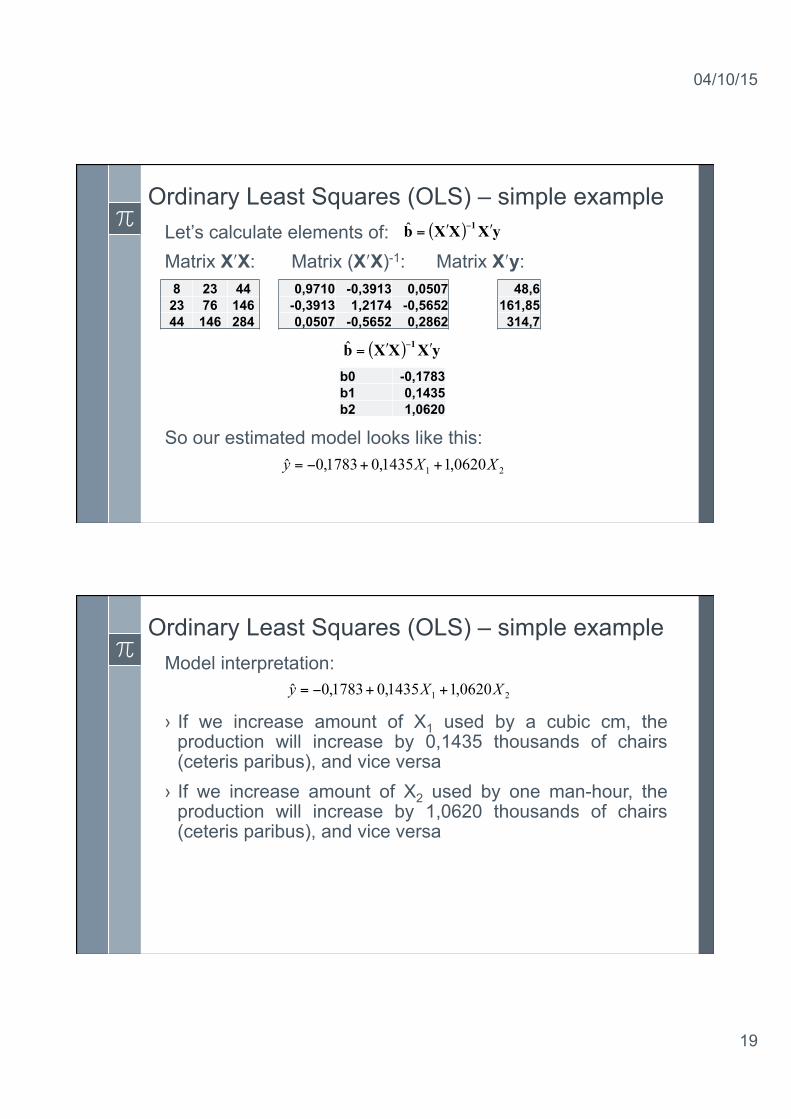
Ordinary Least Squares (OLS) – simple example Let’s calculate elements of: Matrix Xʹ′X: Matrix (Xʹ′X)-1: Matrix Xʹ′y: So our estimated model looks like this:
( ) yXXXb 1 ʹ′ʹ′= −ˆ
8 23 44 23 76 146 44 146 284
0,9710 -0,3913 0,0507 -0,3913 1,2174 -0,5652 0,0507 -0,5652 0,2862
48,6 161,85
314,7
( ) yXXXb 1 ʹ′ʹ′= −ˆ
b0 -0,1783 b1 0,1435 b2 1,0620
21 0620,11435,01783,0ˆ XXy ++−=
Ordinary Least Squares (OLS) – simple example Model interpretation: › If we increase amount of X1 used by a cubic cm, the
production will increase by 0,1435 thousands of chairs (ceteris paribus), and vice versa
› If we increase amount of X2 used by one man-hour, the production will increase by 1,0620 thousands of chairs (ceteris paribus), and vice versa
21 0620,11435,01783,0ˆ XXy ++−=
04/10/15
20
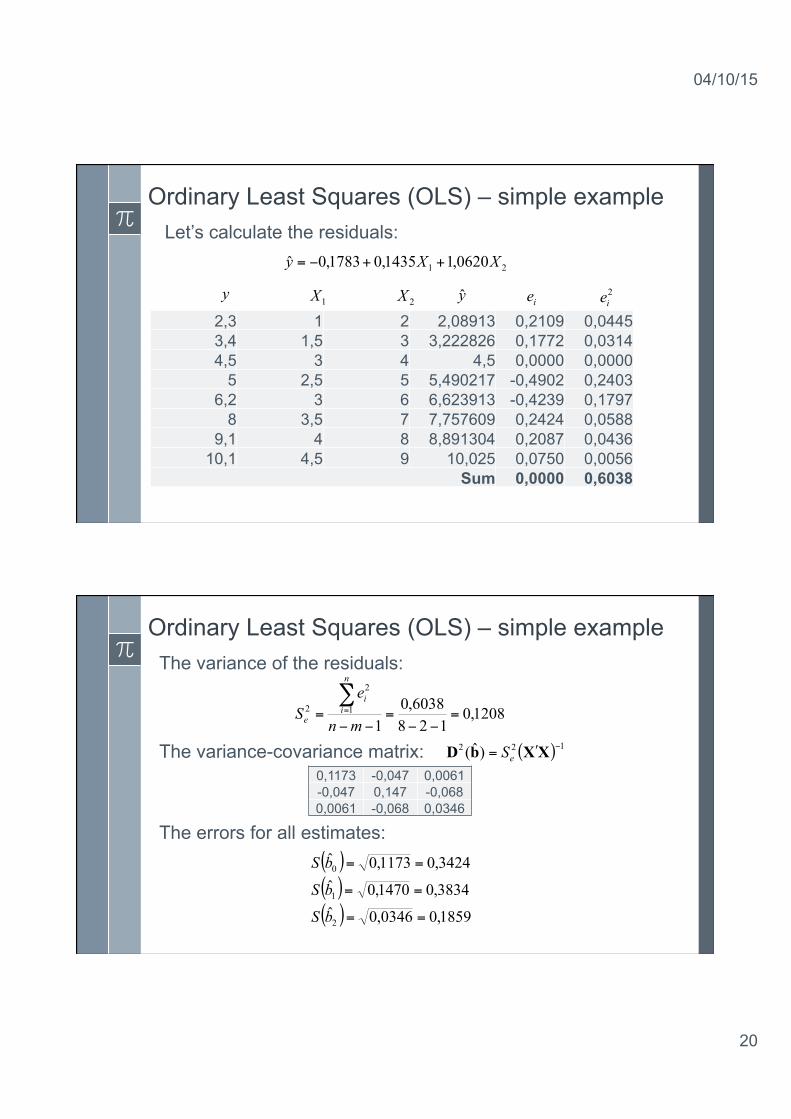
Ordinary Least Squares (OLS) – simple example Let’s calculate the residuals: 21 0620,11435,01783,0ˆ XXy ++−=
y 1X 2X y ie2,3 1 2 2,08913 0,2109 0,0445 3,4 1,5 3 3,222826 0,1772 0,0314 4,5 3 4 4,5 0,0000 0,0000
5 2,5 5 5,490217 -0,4902 0,2403 6,2 3 6 6,623913 -0,4239 0,1797
8 3,5 7 7,757609 0,2424 0,0588 9,1 4 8 8,891304 0,2087 0,0436
10,1 4,5 9 10,025 0,0750 0,0056 Sum 0,0000 0,6038
2ie
Ordinary Least Squares (OLS) – simple example The variance of the residuals:
The variance-covariance matrix:
The errors for all estimates:
1208,0128
6038,01
1
2
2 =−−
=−−
=∑=
mn
eS
n
ii
e
( ) 122 )ˆ( −ʹ′= XXbD eS0,1173 -0,047 0,0061 -0,047 0,147 -0,068 0,0061 -0,068 0,0346
( )( )( ) 1859,00346,0ˆ
3834,01470,0ˆ3424,01173,0ˆ
2
1
0
==
==
==
bS
bS
bS
04/10/15
21
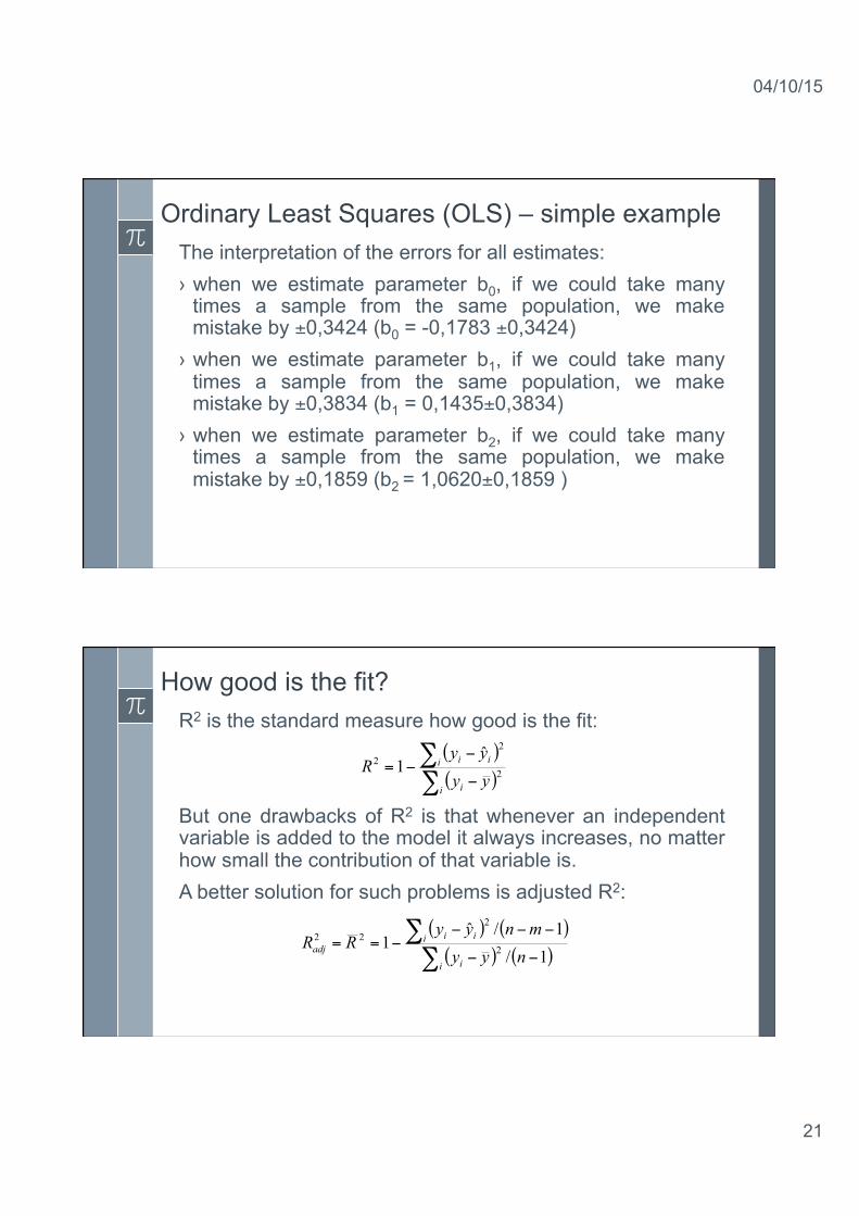
Ordinary Least Squares (OLS) – simple example The interpretation of the errors for all estimates: › when we estimate parameter b0, if we could take many
times a sample from the same population, we make mistake by ±0,3424 (b0 = -0,1783 ±0,3424)
› when we estimate parameter b1, if we could take many times a sample from the same population, we make mistake by ±0,3834 (b1 = 0,1435±0,3834)
› when we estimate parameter b2, if we could take many times a sample from the same population, we make mistake by ±0,1859 (b2 = 1,0620±0,1859 )
How good is the fit? R2 is the standard measure how good is the fit: But one drawbacks of R2 is that whenever an independent variable is added to the model it always increases, no matter how small the contribution of that variable is. A better solution for such problems is adjusted R2:
( )( )∑
∑−
−−=
i i
i ii
yyyy
R 2
22 ˆ1
( ) ( )( ) ( )∑
∑−−
−−−−==
i i
i iiadj nyy
mnyyRR
1/1/ˆ
1 2
222
04/10/15
22
Is the model significant? To make statistical inferences about the goodness of fit of the model or the value of model parameters, we will proceed by assuming that error terms are normally distributed: To test the significance of the overall model we have to test the hypothesis:
To do this we use ratio:
That is distributed as F-statistic with (m, n-m-1) degrees of freedom
( )I0ε 2,N~ σ
0:0:
211
210
≠≠≠
===
m
m
bbbHbbbH…
…
( )( ) ( )∑∑
−−−
−=
i ii
i i
mnyymyy
F1/ˆ
/2
2
Is the model significant? A significant F-statistic does not necessarily mean that all regression model parameters are different from zero. We have to test the hypothesis:
we use the term:
which has a t-distribution with (n-m-1) degrees of freedom
0:0:
1
0
≠
=
i
i
bHbH
( )ii
bSbt ˆˆ
=
04/10/15
23
Detecting problems with the model Multicollinearity
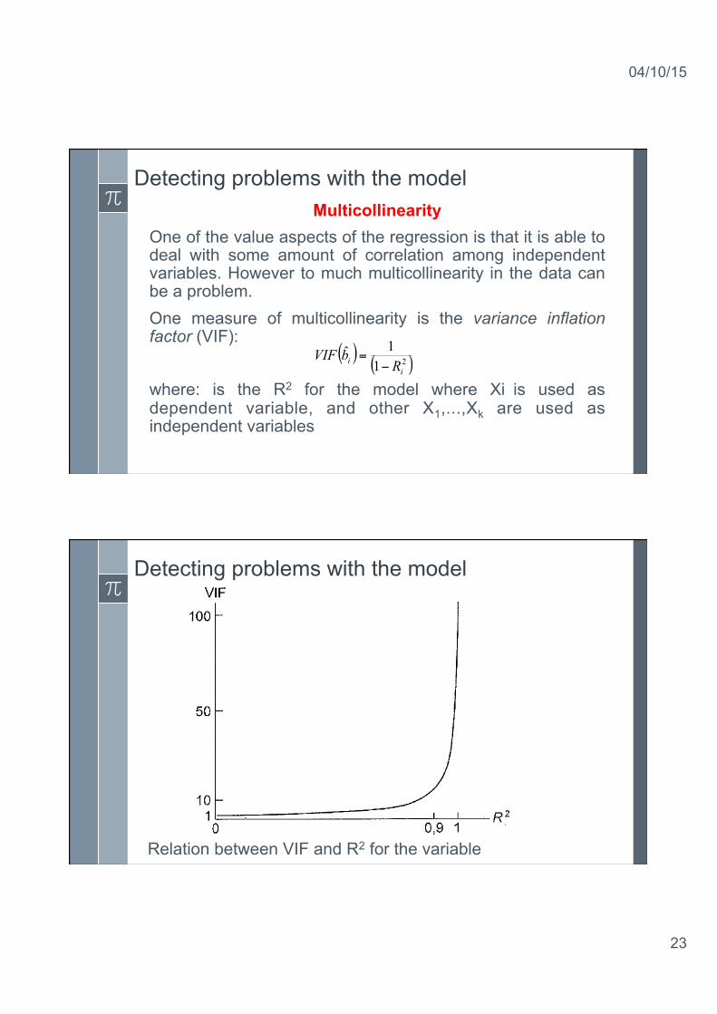
One of the value aspects of the regression is that it is able to deal with some amount of correlation among independent variables. However to much multicollinearity in the data can be a problem. One measure of multicollinearity is the variance inflation factor (VIF): where: is the R2 for the model where Xi is used as dependent variable, and other X1,...,Xk are used as independent variables
( ) ( )211ˆ
ii RbVIF
−=
Detecting problems with the model
Relation between VIF and R2 for the variable
04/10/15
24
Detecting problems with the model Multicollinearity
If we have no multicollinearity in case of one independent variable suggests we have the problem of multicollinearity in our model
( ) 1ˆ =ibVIF
( ) 10ˆ >ibVIF
Detecting problems with the model Heteroscedasticity
As we assume all error terms εi have the same variance σ2. This assumption is called homoscedasticity. When this assumption is violated (i.e. not all variances are the same), we deal with heteroscedasticity. One way do detect heteroscedasticity is the Goldfeld–Quandt test. 1. Divide the sample (size n) in two subsamples A (n1
elements) and B (n2 elements) (n1 + n2 = n). It is possible to omit some observations in the middle of the data – so n1 + n2 < n. We choose the subsamples arbitrary.
04/10/15
25
Detecting problems with the model Heteroscedasticity
2. For each subsample we calculate:
3. We test the hypothesis:
following term is used: which has F-distribution with (n1-m-1, n2-m-1) degrees of freedom
∑∈−−
=Ai
iemns 2
1
21 1
1∑∈−−
=Bi
iemns 2
2
22 1
1
22
211
22
210
:
:
σσ
σσ
>
=
HH
22
21
ssFe =
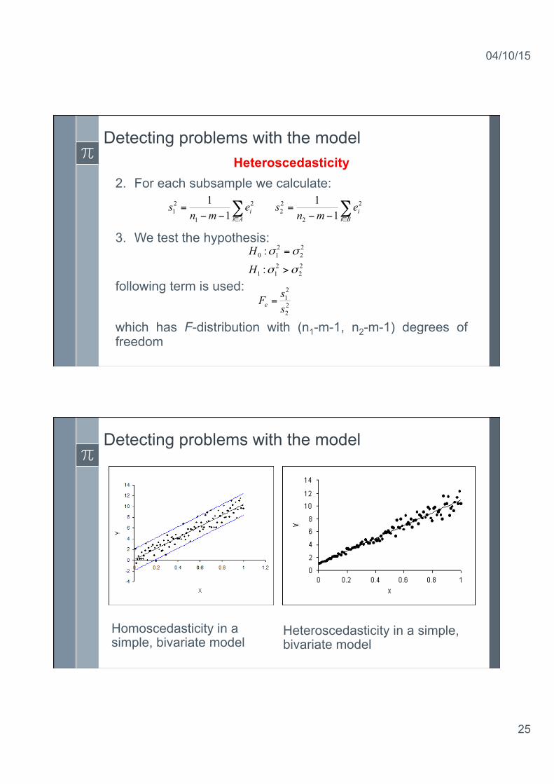
Detecting problems with the model
Homoscedasticity in a simple, bivariate model
Heteroscedasticity in a simple, bivariate model
04/10/15
26
Detecting problems with the model Autocorrelation
To check autocorrelation we have to check the hypothesis:
we use Durbin – Watson statistic (DW) in this case: The null hypothesis tells us there is no autocorrelation, the alternative hypothesis tells us there is a positive autocorrelation
0:0:
1
0
>
=
ρ
ρ
HH
( )
∑∑ −−
=t t
t tt
eee
DW 2
21
Detecting problems with the model Normality of the residuals
To check the normality of the residuals we usually use the Shapiro-Wilk normality test: › Rearrange the data in ascending order xi ≤...≤ xn
› Calculate SS as follows: › If n is even, let m=n/2 if n is odd let m=(n-1)/2 › Calculate b as follows, taking ai weights from Shapiro-Wilk
tables for coefficients:
› Calculate the statistics: › Find p-value in Shapiro-Wilk tables
( )2
1∑ =−=
n
i i xxSS
( )∑ = −+ −=m
i iini xxab1 1
SSbW /2=
04/10/15
27
Regression analysis – packages and functions of R software
Estimation of parameters and confidence intervals for them
stats package – lm, confint functions car package – data.ellipse, confidence.ellipse
Analysis of variance stats package – anova function Basic summaries stats package – summary.lm, extractAIC
Model check stats package – influence.measures, cooks.distance, dfbeta, dfbetas, dffits, hatvalues, rstandard, rstudent
Multicollinearity car package – vif function, DAAG package – vif function perturb package – colldiag function
Testing linearity of the model lmtest package – harvtest function
Normality tests
stats package – shapiro.test function, nortest package – ad.test, cvm.test, lillie.test, sf, test functions lawstat package – rjb.test function
Heteroscedasticity tests lmtest package – gqtest, bptest, hmctest functions
Autocorrelation tests lmtest package – dwtest, bgtest function car package – durbinWatsonTest function
Prediction stats package – predict.lm function
Regression analysis – packages and functions of R software
ESTIMATION lm(formula, data, subset, weights, na.action, method = "qr", model = TRUE, x = FALSE, y = FALSE, qr = TRUE, singular.ok = TRUE, contrasts = NULL, offset, ...)
formula an object of class "formula" (or one that can be coerced to that class): a symbolic description of the model to be fitted.
data n optional data frame, list or environment (or object coercible by as.data.frame to a data frame) containing the variables in the model. If not found in data, the variables are taken from environment(formula), typically the environment from which lm is called.
model, x, y logicals. If TRUE the corresponding components of the fit (the model frame, the model matrix, the response, the QR decomposition) are returned
levels confidence levels
04/10/15
28
Regression analysis – packages and functions of R software
ANALYSIS OF VARIANCE anova(object)
BASIC MODEL SUMMARY summary(object) extractAIC(fit, k=2)
fit fitted model, usually the result of a fitter like lm k=2 numeric specifying the ‘weight’ of the equivalent degrees of
freedom AIC for k=2 and BIC k=log(n) n – numer of observations
Regression analysis – packages and functions of R software
MODEL CHECK influence.measures(model); cooks.distance(model); dfbeta(model); dfbetas(model); dffits(model); hatvalues(model); rstandard(model); rstudent(model)
influence.measures
this suite of functions can be used to compute some of the regression (leave-one-out deletion) diagnostics for linear and generalized linear models discussed in Belsley, Kuh and Welsch (1980), Cook and Weisberg (1982), etc.
cooks.distance
dfbeta
dfbetas
dffits
hatvalues
rstandard
rstudent
model an R object, typically returned by lm or glm
04/10/15
29
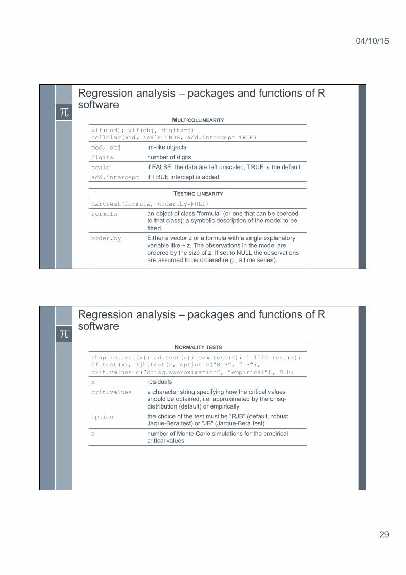
Regression analysis – packages and functions of R software
MULTICOLLINEARITY vif(mod); vif(obj, digits=5) colldiag(mod, scale=TRUE, add.intercept=TRUE)
mod, obj lm-like objects digits number of digits scale if FALSE, the data are left unscaled, TRUE is the default add.intercept if TRUE intercept is added
TESTING LINEARITY harvtest(formula, order.by=NULL)
formula an object of class "formula" (or one that can be coerced to that class): a symbolic description of the model to be fitted.
order.by Either a vector z or a formula with a single explanatory variable like ~ z. The observations in the model are ordered by the size of z. If set to NULL the observations are assumed to be ordered (e.g., a time series).
Regression analysis – packages and functions of R software
NORMALITY TESTS shapiro.test(x); ad.test(x); cvm.test(x); lillie.test(x); sf.test(x); rjb.test(x, option=c(”RJB”, ”JB”), crit.values=c(”chisq.approximation”, ”empirical”), N=0)
x residuals crit.values a character string specifying how the critical values
should be obtained, i.e. approximated by the chisq-distribution (default) or empirically
option the choice of the test must be "RJB" (default, robust Jaque-Bera test) or "JB" (Jarque-Bera test)
N number of Monte Carlo simulations for the empirical critical values
04/10/15
30
Regression analysis – packages and functions of R software
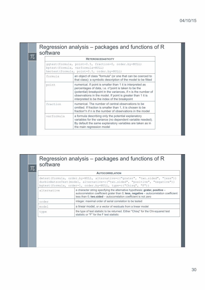
HETEROSCEDASTICITY gqtest(formula, point=0.5, fraction=0, order.by=NULL) bptest(formula, varformula=NULL) hmctest(formula, point=0.5, order.by=NULL)
formula an object of class "formula" (or one that can be coerced to that class): a symbolic description of the model to be fitted
point numerical. If point is smaller than 1 it is interpreted as percentages of data, i.e. n*point is taken to be the (potential) breakpoint in the variances, if n is the number of observations in the model. If point is greater than 1 it is interpreted to be the index of the breakpoint
fraction numerical. The number of central observations to be omitted. If fraction is smaller than 1, it is chosen to be fraction*n if n is the number of observations in the model
varformula a formula describing only the potential explanatory variables for the variance (no dependent variable needed). By default the same explanatory variables are taken as in the main regression model
Regression analysis – packages and functions of R software
AUTOCORRELATION dwtest(formula, order.by=NULL, alternative=c("grater", "two.sided", "less")) durbinWatsonTest(model, alternative=c("two.sided", "positive", "negative")) bgtest(formula, order=1, order.by=NULL, type=c("Chisq", "F"))
alternative a character string specifying the alternative hypothesis: grater, positive – autocorrelation coefficient grater than 0; less, negative – autocorrelation coefficient less than 0; two.sided – autocorrelation coefficient is not zero
order integer. maximal order of serial correlation to be tested
model a linear model, or a vector of residuals from a linear model
type the type of test statistic to be returned. Either "Chisq" for the Chi-squared test statistic or "F" for the F test statistic
04/10/15
31
Regression analysis – packages and functions of R software
PREDICTION
predict(object, newdata, interval="prediction", level=0.95)
object object of class inheriting from "lm" newdata an optional data frame in which to look for variables with which to predict. If
omitted, the fitted values are used
interval type of interval calculation
level tolerance/confidence level
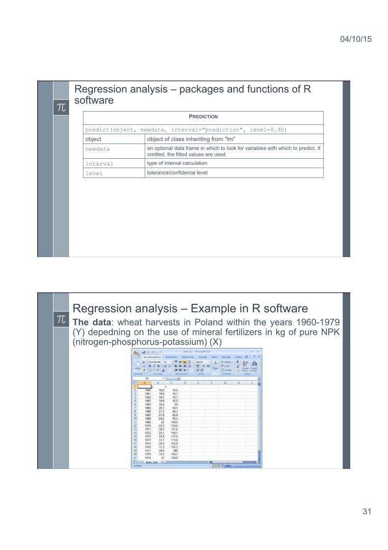
Regression analysis – Example in R software The data: wheat harvests in Poland within the years 1960-1979 (Y) depedning on the use of mineral fertilizers in kg of pure NPK (nitrogen-phosphorus-potassium) (X)
04/10/15
32
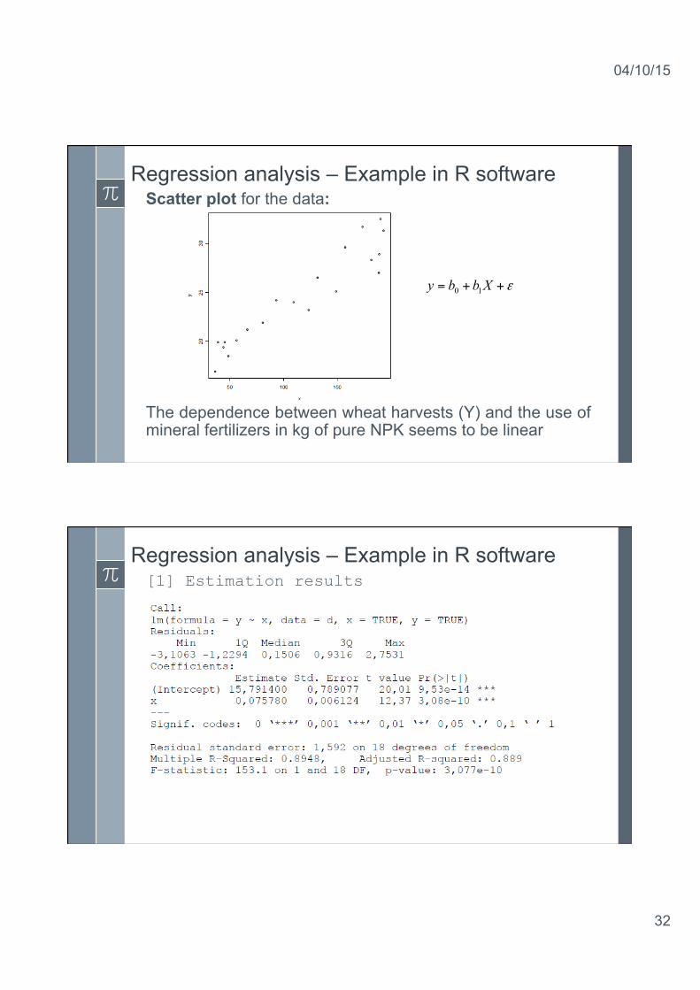
Regression analysis – Example in R software Scatter plot for the data:
The dependence between wheat harvests (Y) and the use of mineral fertilizers in kg of pure NPK seems to be linear
ε++= Xbby 10
Regression analysis – Example in R software [1] Estimation results
04/10/15
33
Regression analysis – Example in R software
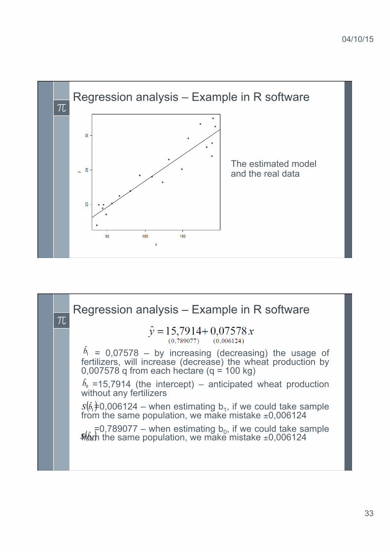
The estimated model and the real data
Regression analysis – Example in R software
= 0,07578 – by increasing (decreasing) the usage of fertilizers, will increase (decrease) the wheat production by 0,007578 q from each hectare (q = 100 kg) =15,7914 (the intercept) – anticipated wheat production without any fertilizers =0,006124 – when estimating b1, if we could take sample from the same population, we make mistake ±0,006124 =0,789077 – when estimating b0, if we could take sample from the same population, we make mistake ±0,006124
1b
0b
( )1bS
( )0bS
04/10/15
34
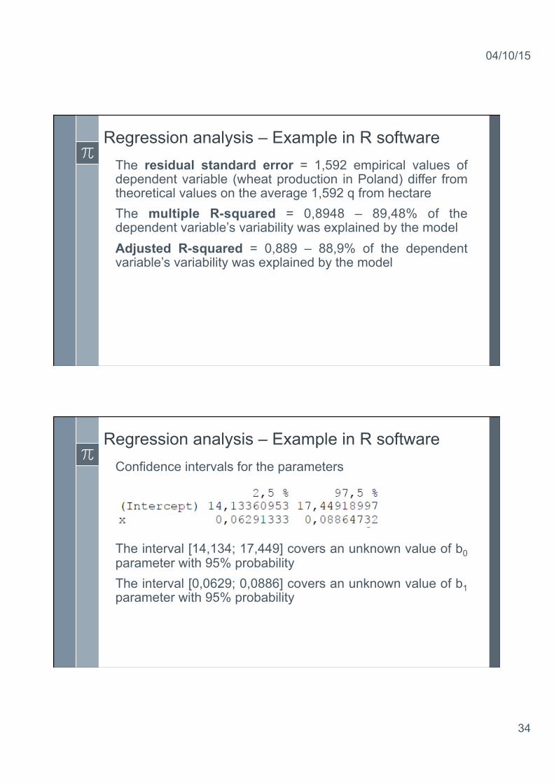
Regression analysis – Example in R software The residual standard error = 1,592 empirical values of dependent variable (wheat production in Poland) differ from theoretical values on the average 1,592 q from hectare The multiple R-squared = 0,8948 – 89,48% of the dependent variable’s variability was explained by the model Adjusted R-squared = 0,889 – 88,9% of the dependent variable’s variability was explained by the model
Regression analysis – Example in R software Confidence intervals for the parameters
The interval [14,134; 17,449] covers an unknown value of b0 parameter with 95% probability The interval [0,0629; 0,0886] covers an unknown value of b1 parameter with 95% probability
04/10/15
35
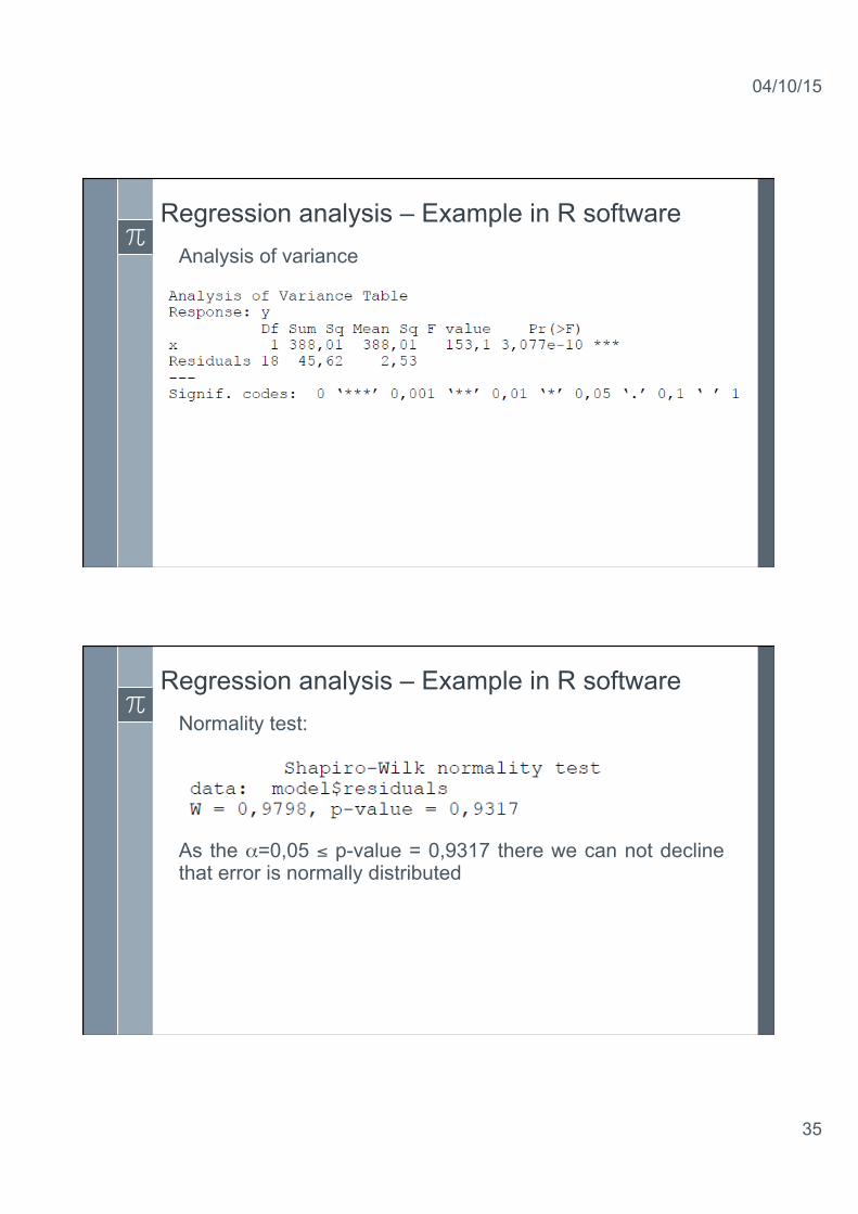
Regression analysis – Example in R software Analysis of variance
Regression analysis – Example in R software Normality test: As the α=0,05 ≤ p-value = 0,9317 there we can not decline that error is normally distributed
04/10/15
36
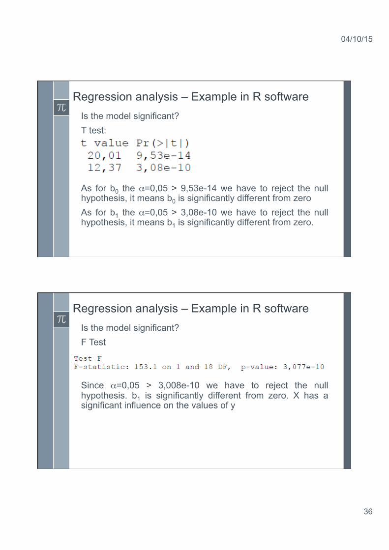
Regression analysis – Example in R software Is the model significant? T test: As for b0 the α=0,05 > 9,53e-14 we have to reject the null hypothesis, it means b0 is significantly different from zero As for b1 the α=0,05 > 3,08e-10 we have to reject the null hypothesis, it means b1 is significantly different from zero.
Regression analysis – Example in R software Is the model significant? F Test Since α=0,05 > 3,008e-10 we have to reject the null hypothesis. b1 is significantly different from zero. X has a significant influence on the values of y
04/10/15
37
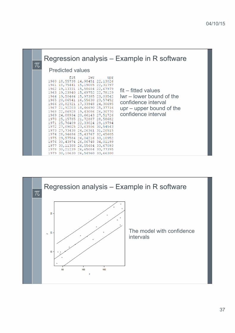
Regression analysis – Example in R software Predicted values
fit – fitted values lwr – lower bound of the confidence interval upr – upper bound of the confidence interval
Regression analysis – Example in R software
The model with confidence intervals

04/10/15
38
Regression analysis – Example in R software Predicted values – new data