regression analysis statistical modeling of a response...

Chapter 5

Multicollinearity

5.1 Introduction

In previous chapters we briefly mentioned a phenomenon calledmulticollinearity, which was defined as the existence of strong correlationsamong the independent variables. The most frequent result of having multi-collinearity when doing a regression analysis is obtaining a very significantoverall regression (small p-value for the F statistic), while the partial coeffi-cients are much less so (much larger p-values for the t statistics). In fact, someof the coefficients may have signs that contradict expectations. Such resultsare obviously of concern because the response variable is strongly related tothe independent variables, but we cannot specify the nature of that relation-ship. That is the reason we devote this long chapter to that topic.

Multicollinearity arises in a multiple regression analysis in several ways.One way is a result of collecting data in an incomplete manner, usually bycollecting only a limited range of data on one or more of the independent vari-ables. The result is an artificially created correlation between two or moreof the independent variables. For example, to predict the cost of a house wemight use the number of square feet of living space and the number of bed-rooms as independent variables. If there a only large houses with many bed-rooms and small houses with few bedrooms (and no small houses with manybedrooms or large houses with few bedrooms, which is not impossible), therewill be a correlation between these two variables that is a function of the waythe data are collected. Another way multicollinearity can arise is to use inde-pendent variables that are naturally correlated. For example, the age of a childand his or her height would be positively correlated as children tend to growas they get older.

So far all of our examples of regression analyses have been based on aspecified model for describing the behavior of the response variable, and the

177

178 Chapter 5 Multicollinearity

regression analyses were performed to confirm the validity of that model.Such analyses are referred to as confirmatory analyses. However, in manystatistical analyses, and especially in regression analyses, the specification ofthe model is somewhat nebulous and a large part of the statistical analysis isdevoted to a search for an appropriate model. Such analyses are referred toas exploratory analyses.

In a regression setting, an exploratory analysis often consists of specifyingan initial model that contains a large number of variables. Because computingconsiderations are no longer a major consideration, the number of variables isoften limited only by data availability, and it is hoped that the statistical analy-sis will magically reveal the correct model. One result of using a large numberof variables is that many of the variables in such a model will be correlatedbecause they may be measuring similar factors.

Now we need to see why multicollinearity creates these difficulties. Mul-ticollinearity is not a violation of assumptions; hence, all statistics obtainedby the analysis are valid. Instead, the problem is that the data are in a senseinadequate to properly estimate the partial coefficients. A partial coefficientis defined as the effect of changing one variable, holding all other variablesconstant. Now, if there is an exact linear relationship between two vari-ables (correlation coefficient, r = 1.0), it is impossible to vary one holdingthe other variable constant, which results in the X′X matrix being singularand so a regression cannot be performed. A correlation of 0.90 is not verydifferent, and although a regression can now be performed, there is verylimited information available of the result of varying one while holding theother constant. As a result, estimates of the coefficients are unreliable or“unstable.”

We can see this difficulty geometrically in Figure 5.1, which shows twocases of data measured on a response variable y and two independent vari-ables x1 and x2. The regression equation would be represented by a plane thatbest fits the data points. Obviously, the plane that fits the data points in (b),the uncorrelated independent variables, would be much more stable over therange of x1 and x2 than would the plane that fits the data points in (a).

Figure 5.1

(a) CorrelatedIndependent Variables(b) UncorrelatedIndependent Variables

y

x1x2

y

x1 x2

5.2 The Effects of Multicollinearity 179

Because multicollinearity is so often encountered, we will devote this entirechapter to this topic. In Section 5.2 we use some artificially generated data toshow how multicollinearity affects the results of a regression analysis. Then,in Section 5.3, we provide some tools to study the existence and nature of themulticollinearity, and in Section 5.4 we present some remedial methods thatmay help to provide useful results.

One very popular method used to combat multicollinearity is the use ofvariable selection, a statistically based method for selecting a subset of theinitially chosen set of independent variables that, ideally, will produce a modelthat has lost very little in precision while being subject to lesser multicollinear-ity. Because this methodology is so often used (and misused) and because itis also used when multicollinearity is not a serious problem, it is presented inChapter 6.

5.2 The Effects of Multicollinearity

We have defined multicollinearity as the existence of correlated independentvariables. The study of multicollinearity in an m variable regression involvesnot only the m(m − 1)/2 pairwise correlations but also the various multiplecorrelations among these variables. In order to provide an introduction to thisobviously messy problem, we start with some simulation studies involvingrelatively simple multicollinearity patterns. We generate data sets of 100 obser-vations using the model:

y = 4.0x1 + 3.5x2 + 3.0x3 + 2.5x4 + 2.0x5 + 1.5x6 + 1.0x7 + ϵ,

where ϵ is the random error. Each of the independent variables has valuesfrom −0.5 to 0.5 generated from the uniform distribution, standardized to havemean of 0 and range of 1. Because all the independent variables have approx-imately equal dispersion, the magnitudes of the coefficients provide an easyvisual guide to the relative importance (degree of statistical significance) ofeach independent variable, with x1 being the most important, x2 the next mostimportant, and so forth.

Three data sets are generated according to these specifications and differonly in the degree and nature of the multicollinearity among independentvariables. In order to provide for easier comparisons among the three sets,the magnitude of the random error is generated to provide an R-square ofapproximately 0.85 for each case.

EXAMPLE 5.1 No Multicollinearity The independent variables in this example are gen-erated with zero population correlations. The purpose of this example is toprovide a basis for comparison with results using data sets havingmulticollinearity. The results of the regression analysis, using PROC REG ofthe SAS System, are shown in Table 5.1.


Table 5.1

Results of Regressionwith no Multicollinearity,Example 5.1

Analysis of Variance

Sum of MeanSource DF Squares Square F Value Pr > F

Model 7 399.05014 57.00716 67.25 <.0001Error 92 77.98936 0.84771Corrected Total 99 477.03951

Root MSE 0.92071 R-Square 0.8365Dependent Mean 0.11929 Adj R-Sq 0.8241Coeff Var 771.81354

Parameter Estimates

Parameter StandardVariable DF Estimate Error t Value Pr > |t|

Intercept 1 0.09419 0.09863 0.95 0.3421X1 1 3.72526 0.32194 11.57 <.0001X2 1 3.78979 0.33785 11.22 <.0001X3 1 3.27429 0.35684 9.18 <.0001X4 1 2.59937 0.32238 8.06 <.0001X5 1 2.04749 0.31101 6.58 <.0001X6 1 1.90056 0.33569 5.66 <.0001X7 1 0.82986 0.34515 2.40 0.0182

The results conform to expectations: the regression is significant (p < 0.0001)and the R-square value is 0.84. The 0.95 confidence intervals for all coefficientsinclude the true parameter values, and the magnitude of the t statistics for test-ing that the coefficients are 0 decrease consistently from x1 to x7. For six of theseven coefficients the p-values suggest a high degree of statistical significance,whereas β7 though significant has by far the largest p-value.

Another feature of regression when there is no multicollinearity is that thetotal and partial regression coefficients are nearly the same. This is shownin Table 5.2, where the first two lines are the partial coefficients and theirstandard errors and the second two lines are the total coefficients and theirstandard errors. Although the partial and total coefficients are not identical,the differences are quite minor. Furthermore, the residual standard deviations(RMSE) of all one-variable models are much larger than those of the multipleregression, indicating that at least several variables are needed.

Table 5.2

Partial and TotalRegression Coefficientswith No Multicollinearity

Variable X1 X2 X3 X4 X5 X6 X7

Partial Coefficient 3.73 3.79 3.27 2.60 2.05 1.90 0.83Standard Error 0.32 0.34 0.36 0.32 0.31 0.34 0.35

Total Coefficient 3.81 2.95 2.87 2.33 1.88 1.57 0.87Standard Error 0.63 0.72 0.78 0.71 0.69 0.76 0.78

EXAMPLE 5.2 “Uniform” Multicollinearity For this example, the independent vari-ables are generated so that correlations between all “adjacent” variables,


that is, between xj and xj+1, are 0.98. Figure 5.2 is a matrix of scatterplots for all pairs of independent variables. The existence of high correla-tions is evident.1 The numbers in the diagonal cells represent the minimumand the maximum value of the variable (recall that the variables all havethe uniform distribution from −0.5 to 0.5). The nature of the correlationsis apparent from these scatter plots.

Figure 5.2

Correlation Matrix ofIndependent Variables,Example 5.2

0.50X1

−0.490.55X2

−0.510.51X3

−0.570.53X4

−0.580.56X5

−0.650.59X6

−0.630.65X7

−0.66

The results of the regression using these data are shown in Table 5.3. TheR-square value is very close to that of the no-multicollinearity case.2 Thereis, however, a big change in the estimated coefficients, and only β6 and β7 arestatistically significant (α = 0.05); this is a surprising result because thesetwo should be the least “important” ones. Furthermore, the estimate of β6 hasa negative sign that does not agree with the true model. Actually, these resultsare a direct consequence of the large standard errors of the estimates of thecoefficients. In general, they are ten to twenty times larger than those result-ing from the no-multicollinearity data. We will see later that a multicollinearityassessment statistic is based on the difference in standard errors.

1Population correlations between xj and xj+2 are 0.982, between xj and xj+3 are 0.983,and so forth.2Because all coefficients are positive, multicollinearity causes the response variable to span alarger range; hence, with a constant R-square, the residual mean square is also larger.


Table 5.3

Results of Regressionwith Multicollinearity,Example 5.2





Parameter Estimates


Intercept 1 −0.08714 0.24900 −0.35 0.7272X1 1 4.87355 3.85464 1.26 0.2093X2 1 3.79018 5.89466 0.64 0.5218X3 1 2.97162 5.85504 0.51 0.6130X4 1 4.96380 5.72319 0.87 0.3880X5 1 0.92972 6.71427 0.14 0.8902X6 1 −12.53227 6.13637 −2.04 0.0440X7 1 13.15390 4.47867 2.94 0.0042

What we have here is the main feature of regression analyses when multi-collinearity is present:

Although the model may fit the data very well, the individual coefficientsmay not be very useful.

In other words, multicollinearity does not affect the overall fit of the modeland therefore does not affect the model’s ability to obtain point estimates ofthe response variable or to estimate the residual variation. However, multi-collinearity does reduce the effectiveness of a regression analysis if itsprimary purpose is to determine the specific effects of the various independentfactor variables. Furthermore, the large standard errors of the coefficients alsoincrease the standard errors of the estimated conditional means and predictedvalues.

When multicollinearity is present, the values of the partial regression coeffi-cients may be quite different from the total regression coefficients as shownin Table 5.4. Here we can see, for example, that the partial coefficient for X1 is4.87, whereas the total coefficient is 17.19! The comparisons of the other coef-ficients show similar results. This is the direct consequence of the definitionsof partial and total regression coefficients: The partial coefficient is the changein µy|x associated with a unit change in the respective x holding constant


all other independent variables, whereas the total coefficient is that changeignoring all other variables. One interesting feature that can be observed hereis that all the estimated total coefficients are very close to 17.5, which is thesum of the seven coefficients in the true model. This is due to the strong corre-lations among all the independent variables. As a result, the model with all vari-ables may not fit the data any better than models with fewer variables if strongmulticollinearity is present.

Table 5.4

Total and PartialRegression Coefficientswith Multicollinearity,Example 5.2

Variables X1 X2 X3 X4 X5 X6 X7

Partial Coefficients 4.87 3.79 2.97 4.96 0.93 −12.5 13.15Standard Errors 3.85 5.89 5.86 5.72 6.71 6.14 4.48

Total Coefficients 17.19 17.86 17.49 17.41 17.20 17.00 17.26Standard Errors 0.82 0.82 0.81 0.81 0.84 0.92 0.90

This is another feature of multicollinearity that is a direct consequence of mul-ticollinearity: correlated variables may be considered as largely measuring thesame phenomenon, therefore one variable may do almost as well as combina-tions of several variables. In this example, the model with all seven variableshas a residual standard deviation (not shown in table) of 2.348, while the indi-vidual single variable regressions have residual mean squares ranging from2.479 to 2.838. Actually, this makes sense, because highly correlated variablestend to provide almost identical information.

In Section 3.4 we presented a method of obtaining partial regression coeffi-cients from residuals, where the coefficients are obtained by performingsimple linear regressions using the residuals from the regression on all otherindependent variables. Multicollinearity implies strong relationships amongthe independent variables that will cause the variance of the residuals fromthese regressions to have small magnitudes. Now the precision of the esti-mated regression coefficient in a simple linear regression (Section 2.3) isinversely related to the dispersion of the independent variable. Since multi-collinearity reduces the dispersion of the residuals, which are the independentvariables in these regressions, the precision of a partial regression coefficientwill be poor in the presence of multicollinearity. We will see later that a multi-collinearity assessment statistic is based on this argument.

Finally, the poor performance of the individual partial coefficients has avery practical explanation. Recall that partial regression coefficients are theeffect due to one variable while holding constant all other variables. But whenvariables are correlated, the data contain very little or no information on whathappens if one variable changes while all others remain constant. In fact, itmay be impossible to change one while keeping others fixed. Hence, the partialcoefficients are trying to estimate something for which there is only limitedinformation at best.


EXAMPLE 5.3 Several Multicollinearities In this example, the population correlationpatterns are more complicated, as follows:

Correlations among x1, x2, and x3 are as in Example 5.2; that is, correla-tions among adjacent variables are 0.98.

Correlations among x4, x5, and x6 are similar to those of Example 5.2,except correlations among adjacent variables are 0.95, but they areuncorrelated with x1, x2, and x3.

Correlations of x7 with all other variables are zero.

The matrix of scatter plots for these data is shown in Figure 5.3 and clearlyshows the high correlations among X1, X2, and X3, somewhat smaller cor-relations among X4, X5, and X6, and the lack of correlation among the rest,particularly X7.

Figure 5.3

Correlation ofIndependent Variables,Example 5.3

0.48X1

−0.490.57X2

−0.560.61X3

−0.640.48X4

−0.490.53X5

−0.550.68X6

−0.590.48X7

−0.49

The results of the regression using these data are shown in Table 5.5.


Table 5.5

Regression Results forExample 5.3




Root MSE 1.64360 R-Square 0.8549Dependent Mean −0.23544 Adj R-Sq 0.8439Coeff Var −698.10234

Parameter Estimates


Intercept 1 0.40158 0.16862 2.38 0.0193X1 1 6.26419 2.92282 2.14 0.0347X2 1 −0.83206 4.22064 −0.20 0.8442X3 1 4.99533 2.84205 1.76 0.0821X4 1 5.03588 1.74862 2.88 0.0049X5 1 −1.36616 2.35952 −0.58 0.5640X6 1 1.95366 1.86944 1.05 0.2987X7 1 2.15221 0.58533 3.68 0.0004

The results are somewhat similar to those of Example 5.2. The statistics forthe model are virtually unchanged: The entire regression is highly significant3

and the standard errors for the coefficients of x1, x2, and x3 are only a littlesmaller than those of Example 5.2. The standard errors for the coefficientsx4, x5, and x6 are significantly smaller than those of Example 5.2 becausethe correlations among these variables are not quite as high. Note, however,that the standard error for the coefficient of x7 is about the same as for theno-multicollinearity case. This result shows that, regardless of the degreeof multicollinearity among variables in the model, the standard error of thecoefficient for a variable not correlated with other variables is not affectedby the multicollinearity among the other variables.

Now that we have seen what multicollinearity can do in a “controlled”situation, we will see what it does in a “real” example.

EXAMPLE 5.4 Basketball Statistics The data are NBA team statistics published by theWorld Almanac and Book of Facts for the 1976/77 through 1978/79 seasons.The following variables are used here:

FGAT Attempted field goalsFGM Field goals madeFTAT Attempted free throwsFTM Free throws madeOFGAT Attempted field goals by opponents

3Again the difference in the magnitudes of the error mean square is due to the larger variationin the values of the response variable.


OFGAL Opponent field goals allowedOFTAT Attempted free throws by opponentsOFTAL Opponent free throws allowedDR Defensive reboundsDRA Defensive rebounds allowedOR Offensive reboundsORA Offensive rebounds allowedWINS Season wins

The data are shown in Table 5.6.

Table 5.6 NBA Data

OBS Region FGAT FGM FTAT FTM OFGAT OFGAL OFTAT OFTAL DR DRA OR ORA WINS

1 1 7322 3511 2732 2012 7920 3575 2074 1561 2752 2448 1293 1416 502 1 7530 3659 2078 1587 7610 3577 2327 1752 2680 2716 974 1163 403 1 7475 3366 2492 1880 7917 3786 1859 1404 2623 2721 1213 1268 304 1 7775 3462 2181 1648 7904 3559 2180 1616 2966 2753 1241 1110 445 1 7222 3096 2274 1673 7074 3279 2488 1863 2547 2937 1157 1149 226 1 7471 3628 2863 2153 7788 3592 2435 1803 2694 2473 1299 1363 557 1 7822 3815 2225 1670 7742 3658 2785 2029 2689 2623 1180 1254 438 1 8004 3547 2304 1652 7620 3544 2830 2135 2595 2996 1306 1312 249 1 7635 3494 2159 1682 7761 3539 2278 1752 2850 2575 1235 1142 32

10 1 7323 3413 2314 1808 7609 3623 2250 1695 2538 2587 1083 1178 2711 1 7873 3819 2428 1785 8011 3804 1897 1406 2768 2541 1309 1178 5412 1 7338 3584 2411 1815 7626 3542 2331 1747 2712 2506 1149 1252 4713 1 7347 3527 2321 1820 7593 3855 2079 1578 2396 2453 1119 1122 2914 1 7523 3464 2613 1904 7306 3507 2861 2160 2370 2667 1241 1234 3715 1 7554 3676 2111 1478 7457 3600 2506 1907 2430 2489 1200 1225 3116 2 7657 3711 2522 2010 8075 3935 2059 1512 2550 2687 1110 1329 4417 2 7325 3535 2103 1656 7356 3424 2252 1746 2632 2232 1254 1121 4918 2 7479 3514 2264 1622 7751 3552 1943 1462 2758 2565 1185 1167 4819 2 7602 3443 2183 1688 7712 3486 2448 1833 2828 2781 1249 1318 3520 2 7176 3279 2451 1836 7137 3409 2527 1909 2512 2533 1244 1121 3121 2 7688 3451 1993 1468 7268 3265 2325 1748 2563 2711 1312 1202 4322 2 7594 3794 2234 1797 8063 3808 1996 1494 2594 2576 1030 1345 5223 2 7772 3580 2655 1887 8065 3767 1895 1437 2815 2683 1349 1166 4424 2 7717 3568 2331 1690 7938 3659 2213 1661 2907 2747 1309 1273 3925 2 7707 3496 2116 1569 7620 3474 2113 1574 2676 2779 1187 1214 4326 2 7691 3523 1896 1467 7404 3571 2238 1699 2421 2525 1301 1195 2827 2 7253 3335 2316 1836 6671 3162 2930 2193 2359 2606 1160 1160 4128 2 7760 3927 2423 1926 7970 3798 2343 1759 2619 2531 1096 1297 4829 2 7498 3726 2330 1845 7625 3795 2211 1627 2504 2315 1256 1186 4730 2 7802 3708 2242 1607 7623 3755 2295 1732 2380 2628 1303 1301 3031 2 7410 3505 2534 1904 6886 3367 2727 2045 2341 2440 1381 1176 4632 2 7511 3517 2409 1848 8039 3864 2246 1666 2676 2664 1234 1486 2633 2 7602 3556 2103 1620 7150 3600 2423 1837 2256 2587 1229 1123 3034 3 7471 3590 2783 2053 7743 3585 2231 1635 2700 2481 1288 1269 5035 3 7792 3764 1960 1442 7539 3561 2543 1933 2495 2637 1169 1317 4436 3 7840 3668 2072 1553 7753 3712 2330 1721 2519 2613 1220 1265 3037 3 7733 3561 2140 1706 7244 3422 2513 1912 2593 2739 1222 1097 4038 3 7840 3522 2297 1714 7629 3599 2252 1705 2584 2770 1409 1378 3639 3 7186 3249 2159 1613 7095 3306 1907 1425 2705 2559 1292 1055 4440 3 7883 3801 2220 1612 7728 3715 2404 1832 2480 2617 1239 1234 44

(Continued)


Table 5.6 (Continued)

OBS Region FGAT FGM FTAT FTM OFGAT OFGAL OFTAT OFTAL DR DRA OR ORA WINS

41 3 7441 3548 2705 2068 7799 3678 2365 1740 2736 2546 1177 1267 4842 3 7731 3601 2262 1775 7521 3564 2635 2004 2632 2684 1208 1232 3143 3 7424 3552 2490 1832 7706 3688 2177 1662 2601 2494 1229 1244 3844 3 7783 3500 2564 1904 7663 3634 2455 1841 2624 2793 1386 1350 3145 3 7041 3330 2471 1863 7273 3565 1980 1466 2577 2367 1248 1065 4046 3 7773 3906 2021 1541 7505 3676 2415 1819 2370 2437 1157 1229 3847 3 7644 3764 2392 1746 7061 3434 2897 2170 2404 2547 1191 1156 4848 3 7311 3517 2841 2046 7616 3631 2277 1713 2596 2429 1307 1218 4749 3 7525 3575 2317 1759 7499 3586 2416 1868 2530 2605 1225 1299 3850 3 7108 3478 2184 1632 7408 3682 2029 1549 2544 2377 1224 1095 3151 4 7537 3623 2515 1917 7404 3408 2514 1889 2703 2510 1260 1197 4952 4 7832 3724 2172 1649 7584 3567 2282 1699 2639 2640 1300 1256 4653 4 7657 3663 1941 1437 7781 3515 1990 1510 2628 2625 1177 1348 5354 4 7249 3406 2345 1791 7192 3320 2525 1903 2493 2594 1059 1180 3455 4 7639 3439 2386 1646 7339 3394 2474 1863 2433 2651 1355 1257 4056 4 7836 3731 2329 1749 7622 3578 2319 1749 2579 2743 1166 1202 4957 4 7672 3734 2095 1576 7880 3648 2050 1529 2647 2599 1136 1365 4558 4 7367 3556 2259 1717 7318 3289 2282 1747 2686 2523 1187 1187 5859 4 7654 3574 2081 1550 7368 3425 2408 1820 2629 2794 1183 1185 4360 4 7715 3445 2352 1675 7377 3384 2203 1670 2601 2600 1456 1121 4761 4 7516 3847 2299 1765 7626 3775 2127 1606 2379 2424 1083 1238 5062 4 7706 3721 2471 1836 7801 3832 2295 1760 2413 2322 1392 1294 4363 4 7397 3827 2088 1606 7848 3797 1931 1415 2557 2486 949 1288 4764 4 7338 3541 2362 1806 7059 3448 2501 1889 2435 2350 1256 1080 4565 4 7484 3504 2298 1732 7509 3475 2108 1567 2591 2453 1310 1156 5266 4 7453 3627 1872 1367 7255 3493 2155 1604 2513 2533 1169 1147 38

We perform a regression of WINS on the other variables for the purpose ofdetermining what aspects of team performance lead to increased wins.

The matrix of scatter plots is shown in Figure 5.4. (Because of space limita-tions, all variable names are truncated to three characters) and the correlation

Figure 5.4

Correlation for NBAData

FGA

FGM

FTA

FTM

OFG

OFG

OFT

OFT

DR

DRA

DR

ORA


coefficients listed in Table 5.7. Note that not all variables are significantlycorrelated. The highest correlations are the obvious ones, between freethrows attempted and made, and somewhat lower correlations are betweenfield goals attempted and made. A few other modest correlations exist, whilemany variables do not appear to be correlated. However, as we will see, thereare indeed other sources of multicollinearity, indicating that absence of highpairwise correlations does not necessarily imply that multicollinearity is notpresent.

Table 5.7 Correlations for NBA Data

FGAT FGM FTAT FTM OFGAT OFGAL OFTAT OFTAL DR DRA OR ORA WINS

FGAT 1 .561** −.238 −.296* .421** .290* .138 .134 .107 .484** .227 .373** .012FGM .561** 1 −.150 −.106 .465** .574** −.038 −.052 −.103 −.222 −.275* .363** .409*FTAT −.238 −.150 1 .941** .191 .174 .058 .033 .152 −.167 .307* .200 .216FTM −.296* −.106 .941** 1 .195 .224 .051 .023 .137 −.229 .138 .185 .221OFGAT .421** .465** .191 .195 1 .786** −.536** −.554** .543** .105 −.102 .604** .157OFGAL .290* .574** .174 .224 .786** 1 −.441** −.455** .033 −.160 −.172 .438** −.057OFTAT .138 −.038 .058 .051 −.536** −.441** 1 .993** −.374** .211 .075 −.011 −.225OFTAL .134 −.052 .033 .023 −.554** −.455** .993** 1 −.392** .200 .091 −.032 −.245*DR .107 −.103 .152 .137 .543** .033 −.374** −.392** 1 .263* .076 .125 .260*DRA .484** −.222 −.167 −.229 .105 −.160 .211 .200 .263* 1 −.001 .232 −.386*OR .227 −.275* .307* .138 −.102 −.172 .075 .091 .076 −.001 1 .002 −.012ORA .373** .363** .200 .185 .604** .438** −.011 −.032 .125 .232 .002 1 .028WINS .012 .409** .216 .221 .157 −.057 −.225 −.245* .260* −.386** −.012 .028 1

∗∗Correlation is significant at the 0.01 level (2-tailed).∗Correlation is significant at the 0.05 level (2-tailed).

The results of the regression using WINS as the dependent variable and all12 performance statistics are shown in Table 5.8. The F -value for the test forthe model as well as the coefficient of determination suggest a rather well-fitting model. However, only two coefficients (FGM and OFGAL) have p-valuesless than 0.01, and one other (FTM) has a p-value less than 0.05. These resultswould suggest that only field goals made by the team and opposition are

Table 5.8

Results of Regression forNBA Data





(Continued)


Table 5.8

(Continued)Parameter Estimates


Intercept 1 36.17379 22.39379 1.62 0.1122FGAT 1 −0.01778 0.01387 −1.28 0.2053FGM 1 0.06980 0.01316 5.31 <.0001FTAT 1 −0.00357 0.01045 −0.34 0.7339FTM 1 0.02767 0.01142 2.42 0.0188OFGAT 1 0.02202 0.01217 1.81 0.0761OFGAL 1 −0.07508 0.01139 −6.59 <.0001OFTAT 1 0.01645 0.01757 0.94 0.3533OFTAL 1 −0.04364 0.02207 −1.98 0.0533DR 1 −0.01376 0.01138 −1.21 0.2317DRA 1 0.00735 0.01274 0.58 0.5667OR 1 0.02654 0.01854 1.43 0.1581ORA 1 −0.02140 0.01393 −1.54 0.1305

important and the coefficients do have the expected sign, while the numberof free throws made by the team has a marginal positive effect.

Results of this nature are, of course, what we expect if multicollinearity ispresent, although these apparent contradictions between model and coeffi-cient statistics are not as severe as those of the artificial examples. Also, wehave seen that another result of multicollinearity is that the partial and totalcoefficients tend to be different. The partial and total coefficients for the NBAdata are shown in Table 5.9. The differences are indeed quite marked, althoughagain not as much as in the artificial data. For example, the three largestt-values in the multiple regression are for field goals and free throws made andopponents field goals allowed, while the three strongest simple regressionsinvolve field goals made, defensive rebounds allowed, defensive rebounds,and opponents, free throws allowed. Also, in this example, single-variable regressions do not fit as well as the multiple regression. However,note that many single-variable regressions have nearly equal residual meansquares.

Table 5.9 Partial and Total Coefficients, NBA Data

Variable FGAT FGM FTAT FTM OFGAT OFGAL OFTAT OFTAL DR DRA OR ORA

Partial Coeff. −.018 0.070 −.004 0.028 0.022 −.075 0.016 −.044 −.014 0.007 0.027 −.021Std. Error 0.014 0.013 0.010 0.011 0.012 0.011 0.018 0.022 0.011 0.013 0.019 0.014|t| 1.282 5.305 0.342 2.424 1.809 6.590 0.936 1.977 1.210 0.576 1.432 1.536

Total Coeff. 0.000 0.022 0.008 0.011 0.004 −.003 −.008 −.011 0.015 −.023 −.001 0.003Std. Error 0.005 0.006 0.005 0.006 0.003 0.006 0.004 0.005 0.007 0.007 0.011 0.012|t| 0.095 3.589 1.767 1.814 1.273 0.457 1.848 2.020 2.150 3.342 0.094 0.223


5.3 Diagnosing Multicollinearity

We have seen the effects of multicollinearity, and if these effects are seenin an analysis, we may conclude that multicollinearity exists. It is use-ful, however, to have additional tools that can indicate the magnitude of(and assist in identifying) the variables involved in the multicollinearity.Two frequently used tools are the variance inflation factor and varianceproportions.

Variance Inflation FactorsIn Section 3.4 we noted that the variance of an estimated partial regressioncoefficient,

Var(βj) = MSE cjj ,

where MSE is the error mean square and cjj is the jth diagonal element of(X ′X)−1. We have already seen that multicollinearity has no effect on theresidual mean square; hence, the large variances of the coefficients must beassociated with large values of the cjj . It can be shown that

cjj =1

(1−R2j )Σi(xj − xj)2

,

where R2j is the coefficient of determination of the “regression” of xj on all

other independent variables in the model. In Chapter 2 we saw that Σt(xj−xj)2

is the denominator of the formula for the variance of the regression coeffi-cient in a simple linear regression. If there is no multicollinearity R2

j = 0,then the variance as well as the estimated coefficient is the same for the totaland partial regression coefficients. However, correlations among any indepen-dent variables causeR2

j to increase, effectively increasing the magnitude of cjjand consequently increasing the variance of the estimated coefficient. In otherwords, the variance of βj is increased or inflated by the quantity [1/(1−R2

j )].This statistic is computed for each coefficient, and the statistics [1/(1−R2

j )],j = 1, 2, . . . , m are known as the variance inflation factors, often simplydenoted by VIF.

We have previously noted that when multicollinearity exists, it is difficultto vary one variable while holding the others constant, thus providing littleinformation on a partial regression coefficient. The variance inflation factorquantifies this effect by stating that the effective dispersion of that indepen-dent variable is reduced by (1−R2

j ), which then increases the variance of thatestimated coefficient.

Table 5.10 shows the variance inflation factors for the three artificial datasets (Examples 5.1, 5.2, and 5.3). From this table we can see the following:

5.3 Diagnosing Multicollinearity 191

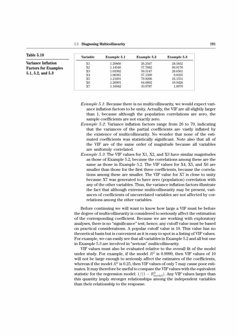
Table 5.10

Variance InflationFactors for Examples5.1, 5.2, and 5.3

Variable Example 5.1 Example 5.2 Example 5.3

X1 1.20860 26.2567 28.5832X2 1.14540 57.7682 60.9170X3 1.03382 59.3147 28.6561X4 1.06381 57.1509 9.0335X5 1.21691 79.0206 16.1551X6 1.26091 64.6862 10.9426X7 1.16042 33.9787 1.0970

Example 5.1: Because there is no multicollinearity, we would expect vari-ance inflation factors to be unity. Actually, the VIF are all slightly largerthan 1, because although the population correlations are zero, thesample coefficients are not exactly zero.

Example 5.2: Variance inflation factors range from 26 to 79, indicatingthat the variances of the partial coefficients are vastly inflated bythe existence of multicollinearity. No wonder that none of the esti-mated coefficients was statistically significant. Note also that all ofthe VIF are of the same order of magnitude because all variablesare uniformly correlated.

Example 5.3: The VIF values for X1, X2, and X3 have similar magnitudesas those of Example 5.2, because the correlations among these are thesame as those in Example 5.2. The VIF values for X4, X5, and X6 aresmaller than those for the first three coefficients, because the correla-tions among these are smaller. The VIF value for X7 is close to unitybecause X7 was generated to have zero (population) correlation withany of the other variables. Thus, the variance inflation factors illustratethe fact that although extreme multicollinearity may be present, vari-ances of coefficients of uncorrelated variables are not affected by cor-relations among the other variables.

Before continuing we will want to know how large a VIF must be beforethe degree of multicollinearity is considered to seriously affect the estimationof the corresponding coefficient. Because we are working with exploratoryanalyses, there is no “significance” test; hence, any cutoff value must be basedon practical considerations. A popular cutoff value is 10. This value has notheoretical basis but is convenient as it is easy to spot in a listing of VIF values.For example, we can easily see that all variables in Example 5.2 and all but onein Example 5.3 are involved in “serious” multicollinearity.

VIF values must also be evaluated relative to the overall fit of the modelunder study. For example, if the model R2 is 0.9999, then VIF values of 10will not be large enough to seriously affect the estimates of the coefficients,whereas if the model R2 is 0.25, then VIF values of only 7 may cause poor esti-mates. It may therefore be useful to compare the VIF values with the equivalentstatistic for the regression model: 1/(1 − R2

model). Any VIF values larger thanthis quantity imply stronger relationships among the independent variablesthan their relationship to the response.


Finally, the effect of sample size is not affected by multicollinearity; hence,variances of regression coefficients based on very large samples may still bequite reliable in spite of multicollinearity.

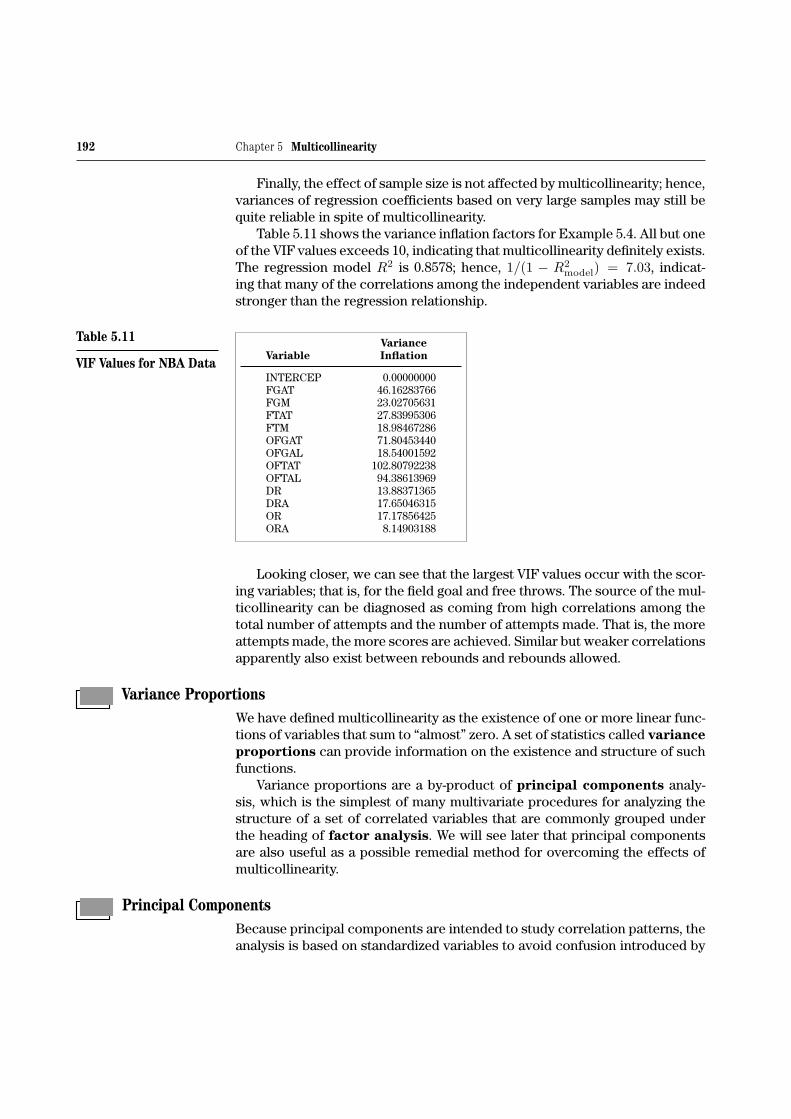
Table 5.11 shows the variance inflation factors for Example 5.4. All but oneof the VIF values exceeds 10, indicating that multicollinearity definitely exists.The regression model R2 is 0.8578; hence, 1/(1 − R2

model) = 7.03, indicat-ing that many of the correlations among the independent variables are indeedstronger than the regression relationship.

Table 5.11

VIF Values for NBA DataVariance

Variable Inflation

INTERCEP 0.00000000FGAT 46.16283766FGM 23.02705631FTAT 27.83995306FTM 18.98467286OFGAT 71.80453440OFGAL 18.54001592OFTAT 102.80792238OFTAL 94.38613969DR 13.88371365DRA 17.65046315OR 17.17856425ORA 8.14903188

Looking closer, we can see that the largest VIF values occur with the scor-ing variables; that is, for the field goal and free throws. The source of the mul-ticollinearity can be diagnosed as coming from high correlations among thetotal number of attempts and the number of attempts made. That is, the moreattempts made, the more scores are achieved. Similar but weaker correlationsapparently also exist between rebounds and rebounds allowed.

Variance ProportionsWe have defined multicollinearity as the existence of one or more linear func-tions of variables that sum to “almost” zero. A set of statistics called varianceproportions can provide information on the existence and structure of suchfunctions.

Variance proportions are a by-product of principal components analy-sis, which is the simplest of many multivariate procedures for analyzing thestructure of a set of correlated variables that are commonly grouped underthe heading of factor analysis. We will see later that principal componentsare also useful as a possible remedial method for overcoming the effects ofmulticollinearity.

Principal ComponentsBecause principal components are intended to study correlation patterns, theanalysis is based on standardized variables to avoid confusion introduced by


differing variances among the variables.4 Thus, if X is an n × m matrix ofobserved standardized variables, then X ′X is the correlation matrix.

Principal component analysis is a procedure that creates a set of new vari-ables, zi, i = 1, 2, . . . , m, which are linearly related to the original set of stan-dardized variables, xi, i = 1, 2, . . . , m. The equations relating the zi to the xi

are of the form

zi = νi1x1 + νi2x2 + · · ·+ νimxm, i = 1, 2, . . . , m,

which can be represented by the matrix equation

Z = XV ,

where V is an m × m matrix of coefficients (νij) that describe the relation-ships between the two sets of variables. The Z variables are called a lineartransformation of the X variables.

There exists an infinite number of such transformations. However, the prin-cipal components transformation creates a unique set of variables, zi, whichhave the following properties:

1. The variables are uncorrelated; that is, Z ′Z is a diagonal matrix with diag-onal elements, λi.

2. z1 has the largest possible variance, z2 the second largest, and so forth.

The principal components transformation is obtained by finding the eigen-values and eigenvectors5 (sometimes called characteristic values and vectors)of the correlation matrix, where the eigenvalues, denoted by λ1, λ2, . . . , λm,are the variances of the corresponding zi, and the matrix of eigenvectors arethe columns of V , the so-called transformation matrix that relates the z vari-ables to the x variables. That is, the first column of V provides the coefficientsfor the equation

z1 = ν11x1 + ν21x2 + · · ·+ νm1xm,

and so forth.We illustrate with the principal components for a sample of 100 observa-

tions from a bivariate population with a correlation of 0.9 between the twovariables. The sample correlation matrix is

X ′X =

!1 0.922

0.922 1

".

The principal component analysis provides the transformation

z1 = 0.707x1 + 0.707x2

z2 = 0.707x1 − 0.707x2,

4In this application, we standardize by subtracting the mean and dividing by the standard devia-tion. In some applications, variables need not be standardized. For simplicity we will not discussthat option.5The theoretical derivation and computation of eigenvalues and eigenvectors are beyond thescope of this book. However, procedures for these computations are readily available in manystatistical software packages.


and the eigenvalues provide the estimated variances of the components:

σ2z1 = 1.922

σ2z2 = 0.078.

The left portion of Figure 5.5 shows a scatter plot of the original variables(labeled X1 and X2), and the right portion shows the scatter plot of the princi-pal component variables (labeled PRIN1 and PRIN2).

Figure 5.5 Two-Variable Principal Components

The plot of the original variables is typical for a pair of highly correlatedstandardized variables. The plot of the principal components is typical of apair of uncorrelated variables, where one variable (PRIN1 in this case) has amuch larger variance. A close inspection shows that the pattern of the datapoints is identical in both plots, illustrating the fact that the principal compo-nent transformation is simply a rigid rotation of axes such that the resultingvariables have zero correlation and, further, that this first component variablehas the largest variance, and so forth.

Note further that the sum of the variances for both sets of variables is 2.0.This result illustrates the fact that the principal component transformation hasnot altered the total variability of the set of variables (as measured by the sum


of variances) but has simply apportioned them differently among the principalcomponent variables.

The eigenvectors show that the first principal component variable consistsof the sum of the two original variables, whereas the second consists of thedifference. This is an expected result: for any two variables, regardless of theircorrelation, the sum provides the most information on their variability, and thedifference explains the rest.

This structure of the principal component variables shows what happensfor different correlation patterns. If the correlation is unity, the sum explainsall of the variability; that is, the variance of the first component is 2.0. Thevariance of the second component is zero because there are no differencesbetween the two variables. If there is little or no correlation, both componentswill have variances near unity.

For larger number of variables, the results are more complex but will havethe following features:

1. The more severe the multicollinearity, the larger the differences inmagnitudes among the variances (eigenvalues) of the components.However, the sum of eigenvalues is always equal to the number ofvariables.

2. The coefficients for the transformation (the eigenvectors) show howthe principal component variables relate to the original variables.

We will see later that the principal component variables with large vari-ances may help to interpret results of a regression where multicollinearityexists. However, when trying to diagnose the reasons for multicollinearity, thefocus is on the principal components with very small variances.

Remember that linear dependencies are defined by the existence of a linearfunction of variables being equal to zero, which will result in one or more prin-cipal components having zero variance. Multicollinearity is a result of “near”linear dependencies among the independent variables that will consequentlyresult in principal components with near zero variances. The coefficients ofthe transformation for those components provide some information on thenature of that multicollinearity. However, a set of related statistics called thevariance proportions are more useful.

Without going into the mathematical details (which are not very instruc-tive), variance proportions indicate the relative contribution from eachprincipal component to the variance of each regression coefficient. Con-sequently, the existence of a relatively large contribution to the variancesof several coefficients by a component with a small eigenvalue (a “near”collinearity) may indicate which variables contribute to the overall multi-collinearity. For easier comparison among coefficients, the variance


proportions are standardized to sum to 1, so that the individual elementsrepresent the proportions of the variance of the coefficient attributableto each component.

The variance proportions for a hypothetical regression using the two cor-related variables we have used to illustrate principal components are shownin Table 5.12 as provided by PROC REG of the SAS System.6

Table 5.12

Variance ProportionsCollinearity Diagnostics (intercept adjusted)

Condition Var Prop Var PropNumber Eigenvalue Index X1 X2

1 1.90119 1.00000 0.0494 0.04942 0.09881 4.38647 0.9506 0.9506

The first column reproduces the eigenvalues and the second the condi-tion indices, which are an indicator of possible roundoff error in computingthe inverse that may occur when there are many variables and multicollinear-ity is extreme. Condition numbers must be very large (usually at least in thehundreds) for roundoff error to be considered a problem.

The columns headed by the names of the independent variables (X1 andX2 in this example) are the variance proportions. We examine these propor-tions looking for components with small eigenvalues, which in this case iscomponent 2 (the variance proportions are 0.9506 for both coefficients). Thesecond principal component consists of the difference between the two vari-ables. The small variance of this component shows that differences betweenthese variables cannot be very large; hence, it is logical that the second com-ponent contributes to the instability of the regression coefficients. In otherwords, the sum of the two variables (the first component) provides almost allthe information needed for the regression.

EXAMPLE 5.3 REVISITED Variance Proportions Table 5.13 shows the eigenvaluesand variance proportions for Example 5.3, which was constructed with twoseparate groups of correlated variables. We can immediately see that thereare three large and four relatively small eigenvalues, indicating rather severemulticollinearity.

6In some references (e.g., Belsley et al., 1980), the variance proportions are obtained by com-puting eigenvalues and eigenvectors from the standardized matrix of uncorrected (raw) sums ofsquares and cross products of the m independent variables and the dummy variable represent-ing the intercept. This procedure implies that the intercept is simply another coefficient that maybe subject to multicollinearity. In most applications, especially where the intercept is beyond therange of the data, the results will be misleading. The subheading “(Intercept adjusted)” in thisoutput shows that the intercept is not included in these statistics.


Table 5.13 Variance Proportions for Example 5.3

Collinearity Diagnostics (intercept adjusted)Condition

Number Eigenvalue Index

1 3.25507 1.000002 2.63944 1.110513 0.92499 1.875904 0.08948 6.031395 0.04440 8.562476 0.03574 9.542937 0.01088 17.29953

Dependent Variable: YCollinearity Diagnostics (intercept adjusted)

Proportion of VariationNo. X1 X2 X3 X4 X5 X6 X7

1 0.00202 0.00095234 0.00211 0.00433 0.00268 0.00353 0.009192 0.00180 0.00087220 0.00167 0.00831 0.00454 0.00711 0.000249073 0.00041184 0.00015092 0.0002104 0.00111 0.0001271 0.0000592 0.949274 0.00016890 0.00023135 0.0004611 0.68888 0.00582 0.43838 0.026855 0.12381 0.00000792 0.14381 0.17955 0.60991 0.30963 0.000235706 0.33377 0.00002554 0.31138 0.11100 0.37663 0.22020 0.014217 0.53803 0.99776 0.54037 0.00682 0.0002887 0.02109 4.683773E-7

Remember that variables involved in multicollinearities are identified byrelatively large variance proportions in principal components with smalleigenvalues (variances). In this example, these are components 5 through 7.We have underlined the larger proportions for these components for eas-ier identification. We can see that variables x1, x2, and x3 have relativelylarge variance proportions in component 7, revealing the strong correlationsamong these three variables. Furthermore, variables x1, x3, x5, and x6 incomponent 6 and x5 and x6 in component 5 show somewhat large propor-tions, and although they do not mirror the built-in correlation pattern, theydo show that these variables are involved in multicollinearities. Variablex7 shows very small proportions in all of these components because it isnot correlated with any other variables but is seen to be primarily involvedwith component 3.

EXAMPLE 5.4 REVISITED Variance Proportions Table 5.14 shows the eigenvaluesand variance proportions for Example 5.4, the NBA data.

Table 5.14 Variance Proportions for NBA Data

Collinearity Diagnostics (intercept adjusted)Condition Var Prop Var Prop Var Prop Var Prop Var Prop

Number Eigenvalue Index FGAT FGM FTAT FTM OFGAT

1 3.54673 1.00000 0.0002 0.0009 0.0001 0.0002 0.00102 2.39231 1.21760 0.0021 0.0018 0.0035 0.0053 0.0000

(Continued)


Table 5.14 (Continued)

Collinearity Diagnostics (intercept adjusted)

Condition Var Prop Var Prop Var Prop Var Prop Var PropNumber Eigenvalue Index FGAT FGM FTAT FTM OFGAT

3 2.09991 1.29961 0.0007 0.0002 0.0030 0.0037 0.00014 1.63382 1.47337 0.0003 0.0052 0.0000 0.0002 0.00015 0.97823 1.90412 0.0021 0.0005 0.0000 0.0011 0.00016 0.59592 2.43962 0.0010 0.0120 0.0001 0.0008 0.00017 0.44689 2.81719 0.0030 0.0010 0.0021 0.0038 0.00008 0.20082 4.20249 0.0054 0.0338 0.0113 0.0095 0.00519 0.05138 8.30854 0.0727 0.1004 0.1756 0.3290 0.0041

10 0.04365 9.01395 0.0204 0.0677 0.1253 0.1563 0.105511 0.00632 23.68160 0.3279 0.3543 0.2128 0.2052 0.215712 0.00403 29.67069 0.5642 0.4221 0.4663 0.2849 0.6682

Var Prop Var Prop Var Prop Var Prop Var Prop Var Prop Var PropNumber OFGAL OFTAT OFTAL DR DRA OR ORA

1 0.0030 0.0004 0.0004 0.0012 0.0000 0.0001 0.00302 0.0000 0.0001 0.0001 0.0003 0.0023 0.0004 0.00093 0.0001 0.0009 0.0009 0.0000 0.0009 0.0016 0.00764 0.0026 0.0001 0.0001 0.0126 0.0096 0.0035 0.00005 0.0001 0.0002 0.0001 0.0023 0.0065 0.0393 0.00356 0.0026 0.0005 0.0004 0.0438 0.0064 0.0013 0.05467 0.0197 0.0001 0.0001 0.0134 0.0235 0.0014 0.11578 0.0877 0.0040 0.0054 0.0158 0.0116 0.0049 0.00449 0.0285 0.0004 0.0000 0.0122 0.0733 0.0177 0.0032

10 0.1370 0.0000 0.0022 0.1040 0.0636 0.0448 0.035811 0.1796 0.3960 0.5324 0.1723 0.3571 0.2832 0.204112 0.5390 0.5974 0.4578 0.6220 0.4452 0.6019 0.5672

There are two very small eigenvalues, indicating two sets of almost lineardependencies. However, the variance proportions associated with theseeigenvalues appear to involve almost all variables, and hence, no sets of corre-lated variables can be determined. Eigenvectors 9 and 10 may also beconsidered small, but there are also no large variance proportions for thesecomponents. In other words, the multicollinearities in this data set appear toinvolve almost all variables.

Inconclusive results from the analysis of variance proportions are quitecommon. However, this analysis is generally available with most computerprograms for regression at small cost in computer resources. Therefore, ifmulticollinearity is suspected, the analysis is worth doing.

5.4 Remedial Methods

We have shown two sets of statistics that may be useful in diagnosing theextent and nature of multicollinearity, and we will now explore various reme-dial methods for lessening the effects of this multicollinearity. The choice ofremedial methods to be employed depends to a large degree on the purpose

5.4 Remedial Methods 199

of the regression analysis. In this context we distinguish between two relatedbut different purposes:

1. Estimation. The purpose of the analysis is to obtain the best estimate ofthe mean of the response variable for a given set of values of the indepen-dent variables without being very concerned with the contribution of theindividual independent variables. That is, we are not particularly interestedin the partial regression coefficients.

2. Analysis of structure. The purpose of the analysis is to determine theeffects of the individual independent variables—that is, the magnitudes andsignificances of the individual partial regression coefficients. We are, ofcourse, also interested in good estimates of the response, because if theoverall estimation is poor, the coefficients may be useless.

If the primary focus of the regression analysis is simply estimating theresponse, then a procedure to delete unnecessary variables from the model,called variable selection, may very well provide the optimum strategy. Andbecause variable selection is used in many applications that do not involvemulticollinearity, it is presented in Chapter 6.

If the purpose of the analysis is to examine structure, however, variableselection is not a good idea because this procedure may arbitrarily delete vari-ables that are important aspects of that structure. Instead we present here twoother remedial methods:

1. Redefining variables2. Biased estimation

Redefining VariablesWe have already shown that one remedy for multicollinearity is to redefine theindependent variables. For example, it is well known that if two variables, say,x1 and x2, are correlated, then the redefined variables

z1 = x1 + x2 and z2 = x1 − x2

may be uncorrelated. In fact, this redefinition (with a change in scale) wasobtained by a principal component analysis for two correlated variables. Now,if these new variables have some useful meaning in the context of the data,their use in the regression provides a model with no multicollinearity. Analy-sis of this model will, however, yield the same overall statistics because thelinear transformation does not affect the overall model. This is easily shownas follows. Given a model with two independent variables

y = β0 + β1x1 + β2x2 + ϵ,

and a model using the z variables

y = α0 + α1z1 + α2z2 + ϵ,

then, using the definitions of the z variables

y = α0 + α1(x1 + x2) + α2(x1 − x2) + ϵ

y = α0 + (α1 + α2)x1 + (α1 − α2)x2 + ϵ.


Thus,

β0 = α0,

β1 = α1 + α2, and

β2 = α1 − α2.

Of course, things are not as simple when there are more than two variables.Two distinct procedures can be used for creating variable redefinitions:

1. Methods based on knowledge of the variables2. Method based on a statistical analysis

Methods Based on Knowledge of the VariablesThe use of linear functions and/or ratios involving the independent variblescan often be employed in providing useful models with reduced multicollinear-ity. For example, the independent variables may be measures of different char-acteristics of, say, a biological organism. In this case, as the total size of theorganism increases, so do the other measurements. Now, if x1 is a measure ofoverall size and the other variables are measurements of width, height, girth,and the like, then using x1 as is and redefining all others as xj /x1 or xj − x1,the resulting variables will exhibit much less multicollinearity. Of course, usingratios will cause some change in the fit of the model, whereas the use of dif-ferences will not.

In other applications the variables may be data from economic time series,where all variables are subject to inflation and increased population and there-fore are correlated. Converting these variables to a deflated and/or per capitabasis will reduce multicollinearity.

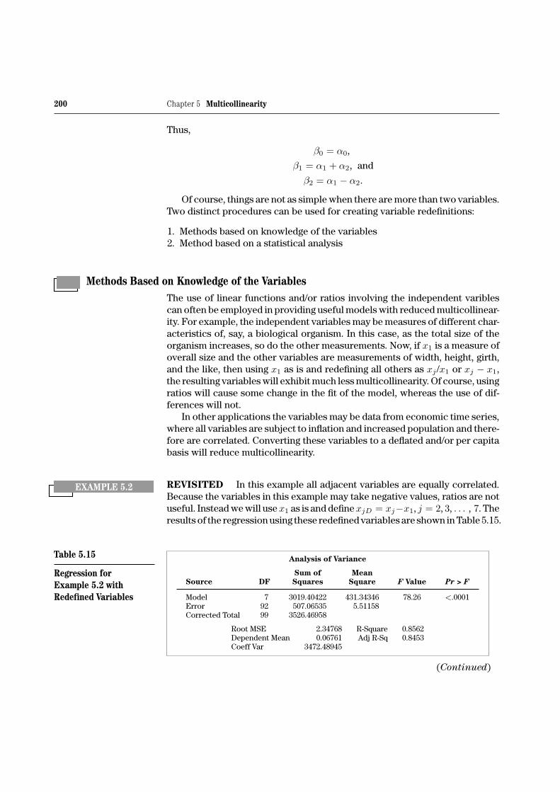
EXAMPLE 5.2 REVISITED In this example all adjacent variables are equally correlated.Because the variables in this example may take negative values, ratios are notuseful. Instead we will usex1 as is and definexjD = xj−x1, j = 2, 3, . . . , 7. Theresults of the regression using these redefined variables are shown in Table 5.15.

Table 5.15

Regression forExample 5.2 withRedefined Variables





(Continued)


Table 5.15


Parameter Standard VarianceVariable DF Estimate Error t Value Pr > |t| Inflation

Intercept 1 −0.08714 0.24900 −0.35 0.7272 0X1 1 18.15049 0.79712 22.77 <.0001 1.12284X2D 1 13.27694 3.97434 3.34 0.0012 1.08797X3D 1 9.48677 4.37921 2.17 0.0329 1.03267X4D 1 6.51515 4.27750 1.52 0.1312 1.05345X5D 1 1.55135 4.48257 0.35 0.7301 1.07297X6D 1 0.62163 4.42548 0.14 0.8886 1.06063X7D 1 13.15390 4.47867 2.94 0.0042 1.03417

A number of features of this analysis are of interest:

1. The overall model statistics are the same because the redefinitions arelinear transformations.

2. The variance inflation factors have been dramatically decreased; the max-imum VIF is now 1.12.

3. The coefficient for X1 now dominates the regression with X2D, X3D, andX7D having some effect (they are significant at the 0.05 level and positive).The rest are not significant. In other words, because the variables are sohighly correlated, the one variable almost does the whole job.

Of course, in this example, as well as in Example 5.3, we know how the vari-ables were constructed. Therefore we have information that allows us to spec-ify appropriate redefinitions needed to reduce the multicollinearity. In mostpractical applications we must use our knowledge of expected relationshipsamong the variables to specify redefinitions.

EXAMPLE 5.4 REVISITED Looking at Figure 5.3 and Table 5.7, we can see that four pairsof variables exhibit a strong bivariate correlation. These are the attemptedand made field goals and free throws for both sides. This correlation seemsreasonable as the more goals a team attempts, the more are made, althoughnot necessarily by the same percentage. Now we know that we can make eachpair of variables uncorrelated by using their sum and difference, but thesevariables make no real sense. Instead, for each pair we will use the numberof attempted goals and the percentages made. The resulting model thus usesthe original four attempted goal numbers, and the rebound numbers and fournew variables:

FGPC, percent of field goals made,FTPC, percent of free throws made,OFGPC, percent of opponent’s field goals made, andOFTPC, percent of opponent’s free throws made.

The matrix of scatter plots for this set of variables is given in Figure 5.6, whichshows that the more serious causes of multicollinearity have been eliminated.


Figure 5.6

Correlation ofIndependent Variables,Example 5.4 Revisited

FGA

FTA

OFG

OFT

DR

DRA

OR

ORA

FGP

FTP

OFG

The results of the regression of WINS on these variables are shown inTable 5.16.

Table 5.16

NBA Regression withRedefined Variables





Parameter Estimates


Intercept 1 91.57717 74.63143 1.23 0.2252 0FGAT 1 0.01639 0.00844 1.94 0.0573 16.62678FGPC 1 5.10633 0.99900 5.11 <.0001 15.57358FTAT 1 0.01743 0.00402 4.33 <.0001 4.01398FTPC 1 0.57673 0.26382 2.19 0.0332 2.16569OFGAT 1 −0.01488 0.00766 −1.94 0.0573 27.65005OFGPC 1 −5.47576 0.85624 −6.40 <.0001 6.98286OFTAT 1 −0.01635 0.00397 −4.12 0.0001 5.11302OFTPC 1 −1.04379 0.51818 −2.01 0.0491 1.26447DR 1 −0.01124 0.01136 −0.99 0.3269 13.46184DRA 1 0.00486 0.01280 0.38 0.7056 17.32192OR 1 0.02288 0.01854 1.23 0.2226 16.71826ORA 1 −0.01916 0.01399 −1.37 0.1765 7.99412


Because we are using ratios rather than linear functions, the overall modelstatistics are not exactly the same as those of the original model; however, thefit of the model is essentially unchanged. The variance inflation factors of mostvariables have decreased markedly, although some are still large enough tosuggest that additional multicollinearity exists. However, the decreased mul-ticollinearity has increased the number of statistically significant coefficients,with three (instead of two) having p-values less than 0.0001 and two others(rather than one) having p-values less than 0.05.

An interesting result is that for both teams, the percentage of field goals andthe attempted free throws are the most important factors affecting the score.This is presumably because the percentages of free throws are more consis-tent than the percentages of field goals. Of more marginal importance are thenumber of attempted field goals of both teams and the percentage of attemptedfree throws by the opposing team. Also, all significant coefficients have theexpected signs.

Methods Based on Statistical AnalysesWhen practical or intuitive redefinitions are not readily available, statisticalanalyses may reveal some useful redefinitions. Statistical analyses of relation-ships among a set of variables are a subset of the field of multivariateanalysis. One of the simplest multivariate methods is principal componentanalysis, which has already been presented as a basis for variance proportions.In our study of variance proportions, we focused on the components havingsmall variances. However, in principal component analysis per se, we focuson those principal components having large eigenvalues.

Remember that principal components consist of a set of uncorrelatedvariables produced by a linear transformation of the original standardized vari-ables, that is,

Z = XV ,

where Z is the matrix of principal component variables, X is the matrix ofstandardized original variables, and V , the matrix of eigenvectors, is the matrixof coefficients for the transformation. Because the original variables have beenstandardized, each has variance 1, and therefore each variable contributesequally to the total variability of the set of variables. The principal compo-nents, however, do not have equal variances. In fact, by construction, the firstcomponent has the maximum possible variance, the second has the secondlargest variance, and so forth. Therefore, principal components with large vari-ances contribute more to the total variability of the model than those withsmaller variances.

The columns of V are coefficients that show how the principal compo-nent variables are related to the original variables. These coefficients mayallow useful interpretations, and if they do, a regression using these uncor-related variables may provide a useful regression with independent variablesthat have no multicollinearity.


Remember that the bivariate sample with correlation of 0.9 producedprincipal components with sample variances of 1.922 and 0.078. This meansthat the first component, zi, accounts for 1.922/2.0 = 0.961 or 96.1% of thetotal variability of the two variables. This is interpreted as saying that virtu-ally all of the variability is contained in one dimension. The variable zi is oftencalled a factor. In situations where there are several variables, it is of interestto do the following:

1. See how many factors account for most of the variability. This generally(but not always) consists of principal components having variances of 1 orgreater.

2. Examine the coefficients of the transformations (the eigenvectors) to seeif the components with large variances have any interpretations relative tothe definitions of the original variables.

EXAMPLE 5.3 REVISITED Principal Components The results of performing a princi-pal component analysis on the data for Example 5.3 are shown in Table 5.17 asproduced by PROC PRINCOMP of the SAS System. The “factors” are labeledPRIN1 through PRIN7 in decreasing order of the eigenvalues. The columnlabeled “Difference” is the difference between the current and next largesteigenvalue; the column labeled “Proportion” is the proportion of total varia-tion (which is m = 7, because each variable has unit variance) accounted forby the current component, and the column labeled “Cumulative” is the sum ofproportions up to the current one.

Table 5.17 Principal Components for Example 5.3

Eigenvalues of the Correlation Matrix

Eigenvalue Difference Proportion Cumulative

1 3.25506883 0.61562926 0.4650 0.46502 2.63943957 1.71444566 0.3771 0.84213 0.92499391 0.83551409 0.1321 0.97424 0.08947982 0.04508195 0.0128 0.98705 0.04439787 0.00865444 0.0063 0.99336 0.03574343 0.02486687 0.0051 0.99847 0.01087656 0.0016 1.0000

Eigenvectors

PRIN1 PRIN2 PRIN3 PRIN4 PRIN5 PRIN6 PRIN7

X1 0.433300 −.368169 −.104350 −.020784 −.396375 0.583956 −.408981X2 0.434555 −.374483 −.092218 0.035511 −.004628 −.007457 0.813070X3 0.443407 −.355409 −.074687 −.034386 0.427738 −.564742 −.410391X4 0.356707 0.445110 −.096324 0.746215 0.268351 0.189315 −.025891X5 0.375671 0.439963 −.043578 −.091719 −.661406 −.466351 −.007122X6 0.354420 0.453307 −.024470 −.655164 0.387846 0.293472 0.050098X7 0.181168 −.026855 0.981454 0.051339 −.003388 0.023601 0.000075

The results show that the first three eigenvalues are much larger than therest. In fact, the cumulative proportions (last column) show that these three


components account for over 97% of the total variation, implying that this setof seven variables essentially has only three dimensions or factors. This resultconfirms that the data were generated to have three uncorrelated setsof variables.

The eigenvectors are the coefficients of the linear equations relating thecomponents to the original variables. These show the following:

1. The first component is an almost equally weighted function of the first sixvariables, with slightly larger coefficients for the first three.

2. The second component consists of the differences between the first andsecond set of three variables.

3. The third component is almost entirely a function of variable seven.

These results do indeed identify three factors:

1. Factor 1 is an overall score that implies that the first six variables are cor-related.

2. Factor 2 is the difference between the two sets of correlated variables.3. Factor 3 is variable 7.

Among these factors, factor 1 by itself does not correspond to the pattern thatgenerated the variables, although it may be argued that in combination withfactor 2 it does. This result illustrates the fact that principal components arenot guaranteed to have useful interpretation.

Because principal components do not always present results that are easilyinterpreted, additional methods have been developed to provide moreuseful results. These methods fall under the topic generally called factor anal-ysis. Most of these methods start with principal components and use variousgeometric rotations to provide for better interpretation. Presentation of thesemethods is beyond the scope of this book. A good discussion of factor analysiscan be found in Johnson and Wichern (2002).

Principal Component RegressionIf a set of principal components has some useful interpretation, it may be pos-sible to use the component variables as independent variables in a regression.That is, we use the model

Y = Zγ + ϵ,

where γ is the vector of regression coefficients.7 The coefficients are estimatedby least squares:

γ = (Z ′Z)−1Z ′Y .

7The principal component variables have zero mean; hence, the intercept is µ and is separatelyestimated by y. If the principal component regression also uses the standardized dependent vari-able, then the intercept is zero.


Since the principal components are uncorrelated, Z′Z is a diagonal matrix,and the variances of the regression coefficients are not affected by multicollinear-ity.8 Table 5.18 shows the results of using the principal components forExample 5.3 in such a regression.

Table 5.18

Principal ComponentRegression, Example 5.3


Sum of MeanSource DF Squares Square F Value Prob > F

Model 7 790.72444 112.96063 44.035 0.0001Error 42 107.74148 2.56527Corrected Total 49 898.46592

Root MSE 1.60165 R-Square 0.8801Dependent Mean 0.46520 Adj R-sq 0.8601Coeff Var 344.29440

Parameter Estimates

Parameter Standard T for H0:Variable DF Estimate Error Parameter = 0 Prob > |t|

INTERCEP 1 0.465197 0.22650710 2.054 0.0463PRIN1 1 2.086977 0.12277745 16.998 0.0001PRIN2 1 −0.499585 0.14730379 −3.392 0.0015PRIN3 1 0.185078 0.23492198 0.788 0.4352PRIN4 1 0.828500 0.77582791 1.068 0.2917PRIN5 1 −1.630063 1.20927168 −1.348 0.1849PRIN6 1 1.754242 1.31667683 1.332 0.1899PRIN7 1 −3.178606 2.02969950 −1.566 0.1248

The results have the following features:

1. The model statistics are identical to those of the original regression becausethe principal components are simply a linear transformation using all of theinformation from the original variables.

2. The only clearly significant coefficients are for components 1 and 2, whichtogether correspond to the structure of the variables. Notice that the coef-ficient for component 3 (which corresponds to the “lone” variable X7) isnot significant.

EXAMPLE 5.4 REVISITED NBA Data, Principal Component Regression Table 5.19shows the results of the principal component analysis of the NBA data, againprovided by PROC PRINCOMP.

8Alternatively, we can compute γ = VB, where B is the vector of regression coefficients usingthe standardized independent variables.


Table 5.19 Principal Component Analysis

Principal Component AnalysisEigenvalues of the Correlation Matrix


PRIN1 3.54673 1.15442 0.295561 0.29556PRIN2 2.39231 0.29241 0.199359 0.49492PRIN3 2.09991 0.46609 0.174992 0.66991PRIN4 1.63382 0.65559 0.136151 0.80606PRIN5 0.97823 0.38231 0.081519 0.88758PRIN6 0.59592 0.14903 0.049660 0.93724PRIN7 0.44689 0.24606 0.037240 0.97448PRIN8 0.20082 0.14945 0.016735 0.99122PRIN9 0.05138 0.00773 0.004282 0.99550PRIN10 0.04365 0.03733 0.003638 0.99914PRIN11 0.00632 0.00230 0.000527 0.99966PRIN12 0.00403 0.000336 1.00000

Eigenvectors

PRIN1 PRIN2 PRIN3 PRIN4 PRIN5 PRIN6

FGAT 0.180742 0.476854 0.266317 0.139942 0.307784 0.169881FGM 0.277100 0.310574 0.106548 −.440931 0.109505 0.405798FTAT 0.090892 −.483628 0.417400 −.003158 −.013379 0.039545FTM 0.101335 −.489356 0.382850 −.087789 −.144502 0.098000OFGAT 0.510884 0.040398 0.090635 0.089731 −.079677 0.062453OFGAL 0.443168 0.020078 0.066332 −.281097 0.045099 −.170165OFTAT −.358807 0.169955 0.434395 −.116152 −.135725 0.171628OFTAL −.369109 0.175132 0.419559 −.116617 −.109270 0.157648DR 0.242131 −.102177 −.029127 0.535598 −.178294 0.602160DRA −.018575 0.309761 0.180227 0.526906 −.335944 −.258506OR −.063989 −.129132 0.236684 0.315635 0.812732 −.116822ORA 0.294223 0.134651 0.360877 0.001297 −.168208 −.514845

PRIN7 PRIN8 PRIN9 PRIN10 PRIN11 PRIN12

FGAT 0.248934 −.222913 −.415273 −.202644 −.309409 −.323937FGM −.101451 −.395466 0.344674 0.260927 0.227146 0.197888FTAT 0.160719 −.250823 0.501105 −.390179 −.193585 −.228698FTM 0.180189 −.190206 −.566482 0.359895 0.156944 0.147620OFGAT −.008903 0.271516 −.123055 −.575011 0.312988 0.439669OFGAL 0.403500 0.571521 0.164850 0.332933 −.145131 −.200655OFTAT −.049914 0.287093 0.048670 0.011021 −.507408 0.497431OFTAL −.054739 0.320340 0.001115 −.095745 0.563739 −.417231DR −.288428 0.209786 0.093180 0.251060 −.123006 −.186518DRA 0.430931 −.203078 0.257780 0.221353 0.199654 0.177923OR −.104360 0.130140 0.124897 0.183196 0.175397 0.204092ORA −.649060 −.085094 −.036331 0.112823 −.102560 −.136459

Because this is a “real” data set, the results are not as obvious as those forthe artificially generated Example 5.3. It appears that the first six componentsare of importance, as they account for almost 94% of the variability. The coef-ficients of these components do not allow very clear interpretation, but the


following tendencies are of interest:

1. The first component is largely a positive function of opponents’ field goalsand a negative function of opponents’ free throws. This may be consideredas a factor describing opponent teams’ prowess on the court rather than onthe free-throw line.

2. The second component is similarly related to the team’s activities on thecourt as opposed to on the free-throw line.

3. The third component stresses team and opponents’ free throws, with someadditional influence of offensive rebounds allowed. This could describe thevariation in total penalties in games.

4. The fourth component is a function of defensive rebounds and a negativefunction of field goals made, and may describe the quality of the defense.

5. The fifth component is almost entirely a function of offensive rebounds.

If we are willing to accept that these components have some useful interpre-tation, we can perform a regression using them. The results are shown inTable 5.20. We first examine the coefficients for the components with largevariances.

Table 5.20

Principal ComponentRegression, NBA Data





Parameter Estimates


Intercept 1 41.00000 0.43369 94.54 <.0001PRIN1 1 1.10060 0.23205 4.74 <.0001PRIN2 1 −1.04485 0.28254 −3.70 0.0005PRIN3 1 −0.15427 0.30157 −0.51 0.6111PRIN4 1 −0.93915 0.34189 −2.75 0.0082PRIN5 1 1.07634 0.44185 2.44 0.0182PRIN6 1 5.43027 0.56611 9.59 <.0001PRIN7 1 −4.18489 0.65372 −6.40 <.0001PRIN8 1 −11.12468 0.97518 −11.41 <.0001PRIN9 1 0.21312 1.92798 0.11 0.9124PRIN10 1 −1.48905 2.09167 −0.71 0.4797PRIN11 1 2.74644 5.49528 0.50 0.6193PRIN12 1 16.64253 6.88504 2.42 0.0191

An interesting feature of this regression is that the three most important coef-ficients (having the smallest p-values) relate to components 6, 7, and 8, whichhave quite small variances and would normally be regarded as relatively


“unimportant” components. This type of result is not overly common, as usu-ally the most important components tend to produce the most important regre-ssion coefficients. However, because of this result, we will need to examinethese components and interpret the corresponding coefficients.

1. Component 6 is a positive function of field goals made and defensiverebounds, and a negative function of offensive rebounds allowed. Its posi-tive and strong contribution to the number of wins appears to make sense.

2. Component 7 is a positive function of opponents’ field goals allowed anddefensive rebounds allowed, and a negative function of offensive reboundsallowed. The negative regression coefficient does make sense.

3. Component 8, which results in the most significant and negative coefficient,is a negative function of all home-team scoring efforts and a positive func-tion of all opponent scoring efforts. Remembering that a double negative ispositive, this one seems obvious.We now continue with the most important components.

4. The first component, which measures the opponent team’s field activityas against its free-throw activity, has a significant and positive coefficient(p < 0.005). When considered in light of the effects of component 8, itmay indicate that when opponents have greater on-court productivity asopposed to free-throw productivity, it helps the “home” team.

5. The second component, which is similar to the first component as appliedto the “home” team, has a significant negative coefficient. It appears thatthese two components mirror each other.

6. Component 3, which relates to free throws by both teams, does not producea significant coefficient.

7. Component 4 indicates that defensive rebounds, both made and allowed,as well as fewer field goals made, contribute positively to the number ofwins. Fortunately, the small value of the coefficient indicates this puzzleris not too important.

8. Component 5, associated with offensive rebounds, is positive.

It is fair to say that although the results do make sense, especially in light of theapparent interplay of component 8 with 1 and 2, the results certainly are notclear-cut. This type of result often occurs with principal component analysesand is the reason for the existence of other factor analysis methods. However,it is recommended that these methods be used with caution as many of theminvolve subjective choices of transformations (or rotations), and thereforep-values must be used carefully.

EXAMPLE 5.5 Mesquite Data Mesquite is a thorny bush that grows in the SouthwesternU.S. Great Plains. Although the use of mesquite chips enhances the flavor ofbarbecue, its presence is very detrimental to livestock pastures. Eliminatingmesquite is very expensive, so it is necessary to have a method to estimatethe total biomass of mesquite in a pasture. One way to do this is to obtain


certain easily measured characteristics of mesquite in a sample of bushes anduse these to estimate biomass:

DIAM1: The wider diameterDIAM2: The narrower diameterTOTHT: The total heightCANHT: The height of the canopyDENS: A measure of the density of the bush

The response is:

LEAFWT: A measure of biomass

Table5.21containsdataonthesemeasuresfromasampleof19mesquitebushes.Figure 5.7 contains the matrix of scatter plots among the five independentvariables, which reveals moderate correlations among all the size variables.

Table 5.21

Mesquite DataOBS DIAM1 DIAM2 TOTHT CANHT DENS LEAFWT

1 2.50 2.3 1.70 1.40 5 723.02 2.00 1.6 1.70 1.40 1 345.03 1.60 1.6 1.60 1.30 1 330.94 1.40 1.0 1.40 1.10 1 163.55 3.20 1.9 1.90 1.50 3 1160.06 1.90 1.8 1.10 0.80 1 386.67 2.40 2.4 1.60 1.10 3 693.58 2.50 1.8 2.00 1.30 7 674.49 2.10 1.5 1.25 0.85 1 217.5

10 2.40 2.2 2.00 1.50 2 771.311 2.40 1.7 1.30 1.20 2 341.712 1.90 1.2 1.45 1.15 2 125.713 2.70 2.5 2.20 1.50 3 462.514 1.30 1.1 0.70 0.70 1 64.515 2.90 2.7 1.90 1.90 1 850.616 2.10 1.0 1.80 1.50 2 226.017 4.10 3.8 2.00 1.50 2 1745.118 2.80 2.5 2.20 1.50 1 908.019 1.27 1.0 0.92 0.62 1 213.5

Figure 5.7

Correlation ofIndependentVariables,Example 5.5

DIAM1

4.10

1.27

DIAM2

3.8

1.0

TOTHT

2.20

0.70

CANHT

1.90

0.62

DENS

7

1


The linear regression of leaf weight on the five measurements produces theresults shown in Table 5.22. The regression is significant, with a p-value of lessthan 0.0001, and the coefficient of determination is reasonably large. However,the residual standard deviation of 180 is quite large compared with the meanleaf weight of 548; hence, there is considerable variability about the estimatedconditional means. When we turn to the coefficients, we see that the varianceinflation factors are not extremely large, yet the smallest p-value for any coef-ficient is 0.014, indicating that the multicollinearity is affecting the precisionof the estimated coefficients. This result is due to the fact that the largest vari-ance inflation factor of 6.0 implies a coefficient of determination of 0.83 forthe relationship of TOTHT to the other variables, which is about the same asthe coefficient of determination for the regression model. In other words, therelationships among the independent variables are essentially as strong as theregression relationship. As we have noted, the effect of multicollinearity isto some degree relative to the strength of the regression; hence, it does havesome effect in this example.

Table 5.22

Regression for MesquiteData



Model 5 2774583 554917 17.14 <.0001Error 13 420823 32371Corrected Total 18 3195406


Parameter Estimates


Intercept 1 −633.94472 174.89405 −3.62 0.0031 0DIAM1 1 421.21444 147.45417 2.86 0.0135 5.89602DIAM2 1 179.01994 125.43117 1.43 0.1771 4.57678TOTHT 1 13.11688 245.54251 0.05 0.9582 6.01963CANHT 1 −110.42797 287.77344 −0.38 0.7074 5.03119DENS 1 −0.19021 31.07269 −0.01 0.9952 1.36574

If the purpose of the analysis is simply to assess the feasibility of estimatingleaf weight, the lack of useful coefficient estimates is not of great concern.However, if we also wish to study how the various measurements affect leafweight, the results of the regression are not particularly useful, and we willwant to try some remedial methods.

We start with a principal component regression. The results of the principalcomponent analysis are shown in Table 5.23, which also includes the correla-tion matrix for the independent variables.


Table 5.23

Principal Componentsfor the Mesquite Data

Principal Component AnalysisCorrelation Matrix

DIAM1 DIAM2 TOTHT CANHT DENS

DIAM1 1.0000 0.8767 0.7255 0.6835 0.3219DIAM2 0.8767 1.0000 0.6354 0.5795 0.2000TOTHT 0.7255 0.6354 1.0000 0.8794 0.3943CANHT 0.6835 0.5795 0.8794 1.0000 0.2237DENS 0.3219 0.2000 0.3943 0.2237 1.0000

Eigenvalues of the Correlation Matrix


PRIN1 3.33309 2.44433 0.666619 0.66662PRIN2 0.88877 0.31655 0.177753 0.84437PRIN3 0.57221 0.45672 0.114443 0.95881PRIN4 0.11550 0.02507 0.023100 0.98191PRIN5 0.09043 . 0.018086 1.00000

Eigenvectors

PRIN1 PRIN2 PRIN3 PRIN4 PRIN5

DIAM1 0.501921 −.124201 0.382765 −.624045 −.443517DIAM2 0.463408 −.261479 0.563632 0.471797 0.420247TOTHT 0.501393 0.045730 −.422215 0.521831 −.544004CANHT 0.474064 −.138510 −.580993 −.339074 0.550957DENS 0.239157 0.946006 0.141387 −.026396 0.164894

The correlation matrix shows high correlations among the two diameter andtwo height variables and somewhat lower correlations between the diameterand height variables. Density appears to be uncorrelated with all other vari-ables. The eigenvalues show one very large eigenvalue and two others thatmay have some importance. The eigenvectors allow the following interpreta-tions of the principal components:

1. The first component is a function of all size variables. This is the size fac-tor and simply shows that larger bushes have larger dimensions. This veryobvious factor also accounts for about two-thirds of the total variability.

2. The second component represents the density, which the correlationsshowed to be an independent factor.

3. The third component has positive coefficients for the diameters and neg-ative coefficients for the heights. Values of this component variable willincrease with diameters and decrease with height; thus, it may be called a“fatness” component.

The results of the principal component regression are shown in Table 5.24. Theregression statistics show that the size component is by far the strongest, butthe fatness component is also important and indicates that short, fat busheshave more leaf weight. Density has no effect, as was seen in the originalregression.


Table 5.24

Principal ComponentRegression for MesquiteData





Parameter EstimatesParameter Standard

Variable DF Estimate Error t Value Pr > |t|

Intercept 1 547.54211 41.27635 13.27 <.0001PRIN1 1 193.05433 23.22834 8.31 <.0001PRIN2 1 −65.36819 44.98294 −1.45 0.1699PRIN3 1 204.38904 56.06126 3.65 0.0030PRIN4 1 −107.18697 124.78284 −0.86 0.4059PRIN5 1 −99.22897 141.02248 −0.70 0.4941

The principal component regression suggests that we may have limited suc-cess with a set of redefined variables. Redefined variables based on know-ledge are usually preferred, as they are more easily interpretable functions ofspecific variables, in contrast to the principal components, which involve allvariables, albeit sometimes with small coefficients. We will try the followingvariables:

SIZE = DIAM1 + DIAM2 + TOTHT + CANHT, a measure of overall sizeFAT = DIAM1 + DIAM2 − TOTHT − CANHT, a measure of fatnessOBLONG = DIAMI − DIAM2, a measure of how oblong, as opposed to

circular, is the shape of the bushHIGH = TOTHT − CANHT, a measure of the size of the stem portion of the

bush9

The results of the regression using these four variables and DENS are shownin Table 5.25.

Table 5.25

Regression withRedefined Variables forMesquite Data

Analysis of VarianceSum of Mean

Source DF Squares Square F Value Pr > F



(Continued)

9Products and ratios could easily have been used and may be more easily justified.


Table 5.25



Intercept 1 −633.94472 174.89405 −3.62 0.0031 0SIZE 1 125.73082 34.06429 3.69 0.0027 2.47971FAT 1 174.38637 61.35209 2.84 0.0139 2.13528OBLONG 1 121.09725 129.28960 0.94 0.3660 1.16344HIGH 1 61.77243 252.43907 0.24 0.8105 1.50442DENS 1 −0.19021 31.07269 −0.01 0.9952 1.36574

Because we have used a complete set of linear transformations, the modelstatistics are identical. The variance inflations show that there is still somemulticollinearity, but it is weaker. The results agree with those of the principalcomponent regression, although the coefficients are not as strong in termsof statistical significance. In other words, the principal component regressionproduced stronger coefficients, which, however, are not as readilyinterpretable.

Biased EstimationThe sampling distribution of a statistic is used to assess the usefulness of astatistic as an estimate of a parameter. The mean of the sampling distributionof the statistic, called the expected value, indicates how well, on the average,the statistic approximates the parameter. The standard deviation of that distri-bution, called the standard error of the estimate, indicates the precision of theestimate. If the expected value is the same as the value of the parameter, theestimate is said to be unbiased, and the smaller the standard error, the moreprecise it is.

In many cases there exist several alternative procedures, called estima-tors, for obtaining an estimate of a parameter. The effectiveness of differentestimators is evaluated on the basis of the expected values and standard errorsof their sampling distributions.

We have made almost exclusive use of the least squares estimator, whichis known to produce unbiased estimates, and among unbiased estimators, itcan be shown to produce the smallest standard errors. Thus, least squares isknown as the best unbiased estimator.10 However, other estimators may beused. For example, the median can be used as an alternative to the mean asa measure of central tendency. In Section 4.4 we introduced the M estimatoras an alternative to the least squares estimator to reduce the effect of outliers.The reason for using alternative estimators is that their sampling distributionsmay have some attractive features.

10Actually, it is known as the best linear unbiased estimator (BLUE) because it is a linear functionof the response variable. The distinction is of no importance here.


For example, suppose that we want to estimate a parameter whose value is100. Two estimators are proposed; one is least squares and the other is some-thing else. Their respective sampling distributions appear in Figure 5.8.

Figure 5.8

Unbiased and BiasedEstimators

The sampling distribution of the least squares estimator is shown by thesolid line. It is seen to be unbiased because its mean is indeed 100, and thestandard error is 10. The alternative estimator is seen to be biased; its meanis 104, but its standard error is smaller: it is 4. The question is, which of theseestimates is “better”?

A widely used statistic for comparing estimators is their mean squarederror, which is defined as the variance plus the square of the bias. In theexample illustrated in Figure 5.8, the least squares estimator has a varianceof 102 = 100 and there is no bias; hence,

Mean squared error = 100 + 0 = 100.

For the alternative estimator the variance is 42 = 16, and the bias is 4; hence,

Mean squared error = 16 + 16 = 32.

Therefore, we may conclude that the biased estimator is “better,” althoughthe usefulness of this result may depend on different penalties for incorrectanswers.

Recent research in remedial methods for combating the effects of mul-ticollinearity has resulted in developing biased estimators for partial regres-sion coefficients that have smaller standard errors. The reduction is obtainedby artificially reducing multicollinearity. Such a procedure, which effectivelyalters the data, results in estimates that are biased. However, this researchhas also found that some of these estimators do have smaller mean squarederrors than does the least squares estimator. Unfortunately, the magnitudes


of the mean squared errors of these estimators are functions of the unknownparameters; hence, it is not possible to know if a particular biased estima-tor does indeed provide that smaller mean squared error. Therefore, resultsobtained by these biased estimation methods should be viewed as exploratoryrather than confirmatory.

Two popular biased estimation methods for multiple regression are ridgeregression and incomplete principal component regression. We presentthebasic formulationforbothof these,butsincetheytendtogivesimilar results,we present an example of only the incomplete principal component estimator.

Ridge RegressionDefine X and Y as the matrices of standardized independent and dependentvariables. The least squares estimator of the regression coefficients is

B = (X ′X)−1X ′Y .

Note that we do not need the dummy variable for the intercept, which is 0 forthe model with standardized variables. The ridge regression estimator is

Bk = (X ′X + kI)−1X ′Y ,

where kI is a diagonal matrix with all elements consisting of an arbitrary smallconstant k. All other statistics are calculated as usual, with the exception thatthe inverse (X ′X + kI)−1 is used in place of (X ′X)−1.

Remember that when all variables are standardized, X ′X is the correlationmatrix with the diagonal elements 1 and the off-diagonal elements the simplecorrelations, rij . However, for the ridge regression estimator, the diagonal ele-ments of X ′X are (1+k), and hence the “effective” correlation between xi andxj now becomes

rij1 + k

,

where rij is the sample correlation between xi and xj . In other words, all cor-relations are artificially reduced by the factor, 1/(1 + k), thereby reducing themulticollinearity. Larger values of k reduce multicollinearity, but increase thebias, whereas a k of zero reproduces the least squares estimates. The questionbecomes one of determining what value of k should be used.

The formulas for calculating the value of k that minimizes the total meansquared error of the set of regression coefficients are functions of the unknownvalues of the population coefficients. Using the least squares coefficients inthese formulas is not advised because multicollinearity makes these estimatesunreliable. The most commonly used procedure is to calculate the ridge regres-sion coefficients for a set of values of k and plot the resulting regressioncoefficients against k. These plots, called ridge plots, often show large changesin the estimated coefficients for smaller values of k, which, as k increases,ultimately “settle down” to a steady progression toward zero. An optimumvalue for k is said to occur when these estimates appear to “settle down.”


EXAMPLE 5.5 REVISITED To illustrate the use of ridge regression, we use the mesquitedata given in Example 5.5.11 A plot of the ridge regression coefficients is shownin Figure 5.9; the plotting symbols 1, 2, T, C, and D represent DIAM1, DIAM2,TOTHT, CANHT, and DENS, respectively. As we noted, determining when thesecoefficients “settle down” is somewhat arbitrary, but a logical choice seems tobe the value 0.75.

Figure 5.9 Ridge Plots for Example 5.5

22 2 2 2 2 2 2 2 2 2 2 2 2 2 2 2 2 2 2 2 2 2 2 2 2 2 2 2 2 2 2 2 2 2

CCC

CC

CC C C C C C C C C C C C C C C C C C C C C C C C C C C

D D D D D D D D D D D D D D D D D D D D D D D D D D D D D D D D D D

1 1 1 1 1 1 1 1 1 1 1 1 1 1 1 1 1 1 1 1 1 1 1 1 1 1 1 1 1 1 1 1 1 1 1

T T T T T T T T T T T T T T T T T T T T T T T T T T T T T T T T T T

COEFFICIENT

Ridge regression control value

300

200

100

0

0 1 2

–100

–200

Using a k of 0.75, the resulting model has a residual standard deviation of 228.6,compared with 179.9 for the least squares regression, a moderate increase thatmay be justified if the coefficients are more useful. The coefficients, their stan-dard errors and t-values are as follows:

VARIABLE COEFF. STD. ERROR T -VALUE

DIAM1 215.5 39.8 5.416DIAM2 185.7 41.1 4.514TOTHT 80.2 65.5 1.223CANHT 61.9 88.7 0.698DENS 8.8 20.9 0.420

11Programs for performing various biased regression analyses are available in many statisticalcomputer packages. In the SAS System they are available as options in PROC REG.


Only the two diameters (DIAM1 and DIAM2) are significant which is certainlya more definitive result.

Incomplete Principal Component RegressionWe have already seen that we can use principal components to provide a regres-sion that may furnish insight into the structure of the regression model. Whenthe regression uses all of the principal components, which we have done, theoverall model is the same as that using the original variables; that is, it pro-duces the same estimates of the response.

We already know that the principal components corresponding to verysmall eigenvalues describe linear combinations of the independent variablesthat are “almost” linearly dependent. In many, but not all, cases, these compo-nents do not contribute to the overall fit of the model. Hence, a model withoutthese components could be useful. However, since the components do notcorrespond to the original variables, the resulting regression is not useful forinferences about the role of the various independent variables. It would, how-ever, be useful to see what this reduced model implies about the regressioncoefficients for the original variables.

Principal components are obtained through a linear transformation of thestandardized independent variables,

Z = XV ,

where Z is the matrix of principal components and V is the matrix of eigen-vectors that are the coefficients of the linear transformation. In principal com-ponent regression, we obtain the estimated model equation

Y = Zγ,

where γ is the set of principal component regression coefficients. Because thisregression is the same as when the original variables have been used, it can beseen that

Y = Zγ = XB,

and

B = V γ.

Incomplete principal component regression uses the above relationship,omitting columns of V corresponding to principal components with very smallvariances that also do not contribute to the regression. That is, if these criteriasuggest keeping only the first p coefficients, then the estimated coefficients forthe original variables can be calculated as

Bp = Vpγp,

where Vp is the matrix containing the first p columns of V and γp is the matrixcontaining the first p principal component regression coefficients. The vari-ances of the estimated coefficients are the diagonal elements of

Var(Bp) = σ2[Vp(Z′pZp)

−1V ′p ],


where Zp is the matrix containing the first p principal component variables.Normally the mean square from the full regression is used as the estimateof σ2, and the square root of the resulting variance is used as a standard errorto provide t statistics. For comparison and interpretive purposes, the coeffi-cients can be converted back to reflect the original units by multiplying thecoefficients by the ratios of the respective standard deviations.

EXAMPLE 5.3 REVISITED A Sampling Experiment In order to provide some ideason the results to be expected from an incomplete principal component regres-sion, we have computed both the ordinary least squares and the incompleteprincipal component regressions, deleting the last four principal componentsfor 250 samples from the population specified for Example 5.3. We delete four(keeping three) because in this example the eigenvalues reflect the known factthat there are three distinct sets of variables. Table 5.26 gives population coef-ficients (BETA) and the means, standard deviations, and standard errors ofthe mean of the resulting empirical sampling distributions of both estimates.

Table 5.26

Sampling Distributionsof RegressionCoefficients,Example 5.3

LEAST SQUARES INCOMPLETE PRINC. COMP.

VARIABLE BETA MEAN STD STD ERR MEAN STD STD ERR

X1 4.0 4.01 5.10 0.32 3.46 0.32 0.020X2 3.5 3.21 7.47 0.47 3.49 0.33 0.021X3 3.0 3.20 5.36 0.34 3.46 0.34 0.021X4 2.5 2.43 2.85 0.18 1.99 0.40 0.025X5 2.0 2.22 4.23 0.26 2.02 0.40 0.025X6 1.5 1.31 3.56 0.23 1.98 0.41 0.026X7 1.0 1.12 1.10 0.07 1.13 1.02 0.064

Using the standard errors, we can see that the means of the least squares coef-ficients are all within the 0.95 confidence intervals of the population values,and the standard deviations clearly show the effects of the high correlationsamong X1, X2, and X3, the more moderate correlations among X4, X5, and X6,and the lack of correlations with X7. This confirms the unbiasedness and largevariances of the least squares estimates.

The incomplete principal components coefficients show an interesting pattern.Therearenowthreedistinctgroups: thefirst three, thesecondthree,andX7.Thecoefficients within the two groups of correlated variables are equivalent in allrespects,andthat forX7 isessentially the leastsquaresestimate. Inotherwords,this method of estimation recognizes the three groups of distinct variables butcannot distinguish among those within a group of correlated variables.

These results are, of course, due to our knowledge of the structure of the datahelping us to choose the number of components to be deleted. In fact, deletingonly three does not provide nearly as informative results. Because the num-ber of “effective” components is rarely known in practical cases, the question


of how many components to delete is not as easily answered. In fact, someauthorities (e.g., Rawlings, 1998, p. 348) caution against eliminating too manycomponents.12 For example, there are no very small eigenvalues in the princi-pal components obtained for Example 5.5, and therefore an incomplete prin-cipal component regression may not be suitable for this data set.

EXAMPLE 5.4 REVISITED Incomplete Principal Component Regression (IPC) onNBA Data The results of the principal component regression would seemto indicate that incomplete principal component regression may not be usefulas some of the components with small variances appeared to be useful in theregression. Because IPC regressions are relatively easy to do, we requestedPROC REG to compute such regressions leaving out 1, 2, . . . ,7 principal com-ponents and the plotted residual standard deviation (root mean squared error)against the number of components omitted, which is shown in Figure 5.10.

Figure 5.10

Plot of RMSE vs Numberof Principal ComponentsDropped for Example 5.4

Root mean squared error9

8

7

6

5

4

3

1 2 3 4 5 6 7 8 9

Number of principal components dropped

+ + +

+

+

+ + +

+

This plot clearly shows that four components can be deleted without affectingthe fit of the regression. Table 5.27 shows the resulting coefficients and relatedstatistics for that regression as well as the ordinary least squares results. Notethat now virtually all coefficients may be considered statistically significant,and all have the expected signs and appear to conform to expectations. Thus, itappears that the incomplete principal component regression has provided use-ful information on the importance of the individual independent variables.

12Considering the relatively low cost of computing, it may not be unreasonable to examine theresults of different numbers of deleted components.

5.5 Summary 221

Table 5.27 Incomplete Principal Component Regression for NBA Data

Least Squares Incomplete P.C. Regression

Variable Coefficient Std.Err. t Coefficient Std.Err. t

Intercept 36.1738 22.3938 1.61535 35.3140 21.2638 1.6608FGAT −0.0178 0.0139 −1.28238 0.0104 0.0017 6.0178FGM 0.0698 0.0132 5.30537 0.0472 0.0032 14.8988FTAT −0.0036 0.0104 −0.34174 0.0130 0.0015 8.5811FTM 0.0277 0.0114 2.42418 0.0143 0.0018 7.8020OFGAT 0.0220 0.0122 1.80894 −0.0076 0.0010 −7.5865OFGAL −0.0751 0.0114 −6.58993 −0.0497 0.0040 −12.5231OFTAT 0.0165 0.0176 0.93645 −0.0108 0.0014 −7.6900OFTAL −0.0436 0.0221 −1.97690 −0.0163 0.0020 −8.3107DR −0.0138 0.0114 −1.20982 0.0128 0.0035 3.6644DRA 0.0073 0.0127 0.57649 −0.0151 0.0032 −4.6989OR 0.0265 0.0185 1.43163 −0.0106 0.0043 −2.4472ORA −0.0214 0.0139 −1.53594 0.0091 0.0062 1.4616

5.5 Summary

This chapter considers a data condition called multicollinearity, which isdefined as the existence of strong correlations among the independent vari-ables of a regression model. Although multicollinearity is not strictly a viola-tion of assumptions, its presence does decrease the precision of the estimatedregression coefficients, thereby making interpretations more difficult.

The existence and nature of multicollinearity are studied by usingvariance inflation factors and variance proportions. Additional informationcan be obtained through the use of principal components, as well as othermultivariate analyses that are not covered in this book.

Because multicollinearity is often caused by having too many independentvariables in the model, it is tempting to “solve” the multicollinearity prob-lem by using a statistically based variable selection procedure. Although thismethod will usually provide models with less multicollinearity, it may not pro-vide insight into the structure of the regression relationships. And becausevariable selection is actually more useful when multicollinearities are not pre-sent, its presentation is deferred to Chapter 6.

In this chapter we presented several remedial methods that may be used toprovide additional information about the structure of the regressionrelationships:

1. The use of information about known relationships to redefine variables inthe model.

2. The use of the results of principal components to create a new set of inde-pendent variables. Similar procedures are available using other multivari-ate methods.


3. The use of biased estimation methods. The methods discussed here includethe incomplete principal component regression and the ridge regression.

The reader may be frustrated by the lack of definitive results of the use ofthese methods on the “real” data examples in this chapter. Unfortunately, thiswill be an almost universal occurrence, because we are dealing with situationswhere the data are simply inadequate to obtain the desired results.

5.6 CHAPTER EXERCISES

In each of these exercises there is some degree of multicollinearity. For eachexercise:

1. Determine the extent and nature of the multicollinearity.2. Discuss possible practical reasons why the multicollinearity exists.3. Implement at least one form of remedial action and determine if these

methods provided more useful results.

1. In Exercise 2 of Chapter 3 we used data from a set of tournaments featur-ing professional putters. In that exercise we related players’ “Player of theYear” point scores to various variables characterizing the players’ perfor-mances. At the end of the tour there is an “auction” that places a “price” onthe players. In this exercise we will estimate the price using a regressionwith the following independent variables:

TNMT: The number of tournaments in which the player participatedWINS: The number of tournaments wonAVGMON: Average money won per tournamentPNTS: The number of “Player of the Year” points accumulated by the

playerASA: The player’s “adjusted” point average; the adjustment reflects the

difficulties of the courses played

The data set is in File REG05P01.

2. In Exercise 1 of Chapter 3 we related gasoline mileage (MPG) to severalcharacteristics of cars:

WT: Weight in poundsESIZE: Engine piston displacement in cubic inchesHP: Engine horsepower ratingBARR: Number of barrels in carburetor

There is already a modest amount of multicollinearity among these vari-ables. For this exercise we add another variable:

TIME: Time taken to a quarter mile from a dead stop (in seconds)

This additional variable creates somewhat greater multicollinearity. Thedata set is in File REG05P02.

5.6 Chapter Exercises 223

3. Pork bellies are a surprisingly valuable portion of a pig, as indicated by thefact that prices of pork bellies are frequently quoted in the media. This meansthat their price is a factor in the price of the pig carcass. Unfortunately, theweight of this item is not readily discerned from an examination of the wholecarcass as it is in the process of being sold, and there is interest in beingable to estimate pork-belly weight based on some more readily available car-cass dimensions. We will therefore investigate a regression to estimate bellyweight (BELWT) from the following measurements:

AVBF: Average of three measures of back fat thicknessMUS: A muscling score for the carcass; higher numbers mean relatively

more muscleLEA: The loin areaDEP: Average of three measures of fat opposite the tenth ribLWT: Live weight of the carcassCWT: Weight of the slaughtered carcassWTWAT: A measure of specific gravity of the carcassDPSL: Average of three determinations of the depth of the bellyLESL: Average of three measures of leanness of belly cross-sections

Obviously, many of these variables are correlated. The data on 48 carcassesare available in File REG05P03.

4. Water evaporation is a major concern in planning irrigation. Data are col-lected daily from June 6 through July 21 in a central Texas location on thefollowing variables that may affect the amount of evaporation:

MAXAT: Maximum daily air temperatureMINAT: Minimum daily air temperatureAVAT: The integrated area under the daily air temperature curve, a

measure of average air temperatureMAXST: Maximum daily soil temperatureMINST: Minimum daily soil temperatureAVST: The integrated area under the daily soil temperature curve, a

measure of average soil temperatureMAXH: Maximum daily humidityMINH: Minimum daily humidityAVH: The integrated area under the daily humidity curve, a measure of

average humidityWIND: Total wind, measured in miles per day

The response is:

EVAP: Daily total evaporation from soil

The data are in File REG05P04. The natural grouping of variables (MAX,MIN, AV) of three factors would appear to provide for redefining variables,either by using common sense or principal components.


5. Data on the following variables are obtained from the U.S. Bureau of theCensus State and Metropolitan Area Data Book, 1986 (A StatisticalAbstract Supplement) and given in File REG05P05. A set of 53 primarymetropolitan areas (PMSAs) are selected for this data set. The variablesare as follows:

PMSA: Identification of PMSAAREA: Land area in square milesPOP: Total population, 1980, in thousandsYOUNG: 1980 population ages 18–24 in thousandsDIV: Total number of divorces in 1982 in thousandsOLD: 1982 total number of Social Security benefit recipients in

thousandsEDUC: Number of adults, 25 years or older, having completed 12 or

more years of schoolPOV: Total number of persons below poverty level in 1979UNEMP: Total number unemployed, 1980CRIME: Total number of serious crimes in 1980

The purpose of the analysis is to determine factors affecting crime. Theindependent variables as presented have a high degree of multicollinearity.There is, however, a good reason for this and determining the reason beforeperforming any analyses should be helpful in developing remedial action.

6. Exercise 4 of Chapter 4 dealt with factors affecting state expenditures oncriminal activities (courts, police, etc.):

STATE: The standard two-letter abbreviation (DC is included)EXPEND: State expenditures on criminal activities ($1000)BAD: The number of persons under criminal supervisionCRIME: Crime rate per 100,000LAWYERS: The number of lawyers in the stateEMPLOY: The number of persons employed in the statePOP: The population of the state (1000)

The data are available in File REG04P04. Examine for multicollinearityand, if necessary, implement remedial procedures both with and withoutpossible outliers and/or influential observations found in that data set.Comment on results.

7. Freund and Wilson (2003) give an example where the size of squid eatenby sharks and tuna is to be estimated based on dimensions of the beaks(mouth). The beaks are indigestible and can be recovered and used to esti-mate the weight of the squid. To do this, a sample of 22 specimens wastaken and the following measurements were taken:

WT: Weight (response variable)RL: Rostral length

5.6 Chapter Exercises 225

WL: Wing lengthRNL: Rostral to notch lengthNWL: Notch to wing lengthW: Width

Because of the nature of the response variable, it was decided that naturallogarithm of the original data would be appropriate for the analysis. Thedata are given in Table 5.28 and File REG05P07.

Table 5.28

Data for Exercise 7OBS RL WL RNL NWL W WT

1 0.27003 0.06766 −0.82098 −0.28768 −1.04982 0.667832 0.43825 0.39878 −0.63488 −0.10536 −0.75502 1.064713 −0.01005 −0.17435 −1.07881 −0.56212 −1.13943 −0.328504 −0.01005 −0.18633 −1.07881 −0.61619 −1.30933 −0.210725 0.04879 −0.10536 −1.02165 −0.44629 −1.20397 0.086186 0.08618 −0.07257 −0.86750 −0.49430 −1.17118 0.198857 0.07696 −0.10536 −0.91629 −0.67334 −1.17118 0.019808 0.23902 0.07696 −0.82098 −0.26136 −1.07881 0.657529 −0.01005 −0.16252 −1.02165 −0.57982 −1.23787 −0.44629

10 0.29267 0.12222 −0.79851 −0.26136 −0.99425 0.7323711 0.26236 0.09531 −0.79851 −0.27444 −0.96758 0.6831012 0.28518 0.09531 −0.73397 −0.26136 −0.96758 0.6418513 0.62058 0.38526 −0.51083 0.00995 −0.43078 2.1471014 0.45742 0.29267 −0.65393 −0.05129 −0.69315 1.5018515 0.67803 0.46373 −0.40048 0.18232 −0.52763 2.1388916 0.58779 0.44469 −0.41552 0.01980 −0.52763 1.8197017 0.55962 0.45742 −0.46204 0.08618 −0.52763 2.0202218 0.54232 0.35767 −0.44629 0.01980 −0.46204 1.8500319 0.51879 0.45108 −0.32850 −0.04082 −0.38566 2.0320920 0.55962 0.46373 −0.38566 0.07696 −0.47804 2.0515621 0.78390 0.62058 −0.28768 0.21511 −0.32850 2.3174722 0.54812 0.51282 −0.44629 0.13103 −0.59784 1.92862

(a) Use the data as is and perform the regression.(b) Retain the variable W and express the rest as ratios of this value. Per-

form the regression. Compare it to the results in (a).(c) Perform a principal component analysis and evaluate it.(d) Perform the regression on the principal components found in (c).(e) Can any of the principal components be omitted from the analysis? If

so, perform the regression without them. Explain the results.

regression analysis statistical modeling of a response...

Documents