linear stability analysis, dynamic response, and design of ... · shimmy dampers for main landing...

Linear Stability Analysis, Dynamic Response, and Design of Shimmy Dampers for Main

Landing Gears

by

Carlos Arreaza

A thesis submitted in conformity with the requirements for the degree of Master of Applied Science

Graduate Department of Mechanical and Industrial Engineering

University of Toronto

© Copyright by Carlos Arreaza 2015

ii

Abstract

Linear Stability Analysis, Dynamics Response, and Design of

Shimmy Dampers for Main Landing Gears

Carlos Arreaza

Master of Applied Science

Graduate Department of Mechanical and Industrial Engineering

University of Toronto

2015

This thesis presents the linear stability analysis and dynamic response of shimmy dampers for main

landing gears. The stability analysis is performed using a single tire landing gear model along with the

dynamics of the shimmy dampers and the stretched string tire model. The dynamic response of each

damper is obtained through a multibody model developed in MSC Adams and validated using existing

literature. Two shimmy dampers are the focus of this study, one developed by Boeing and the other by

UTC Aerospace systems. Finally, a new and improved shimmy damper is proposed showing the stability

regions and its dynamic response. The proposed damper is lighter, easier to manufacture, to install, and to

maintain, and has an overall better dynamic performance.

iii

Acknowledgements

I would like to acknowledge my supervisors Professor Jean Zu and Professor Kamran Behdinan for

giving me the help, support, and guidance needed to finish this thesis throughout my master’s degree at

the University of Toronto. Without their help, it would have been extremely hard and merely impossible

to finish my work. Their technical guidance, moral support, and experience helped me reach my goals and

be able to accomplish this work.

I would also like to thank my lab mates in the VDML group for their help, support, and company. I

learned a lot by being part of the team, and listening to their interesting projects and wisdom. Their aid

was also indispensable for the successful completion of this work.

Finally, I thank my family for their support and constant motivation. They were always there when I

needed them, and I definitely couldn’t have done it without them.

iv

Table of Contents

Chapter 1 Introduction .................................................................................................................................. 1

1.1 Causes of shimmy ............................................................................................................................... 1

1.2 Landing gear mechanical models ........................................................................................................ 3

1.2.1 Third-order model: simple trailing wheel system with yaw DOF ............................................... 3

1.2.2 Fifth-order model: yaw and lateral DOF ...................................................................................... 3

1.2.3 Seventh-order model: fifth-order system with steering................................................................ 4

1.3 Vehicle dynamics ................................................................................................................................ 4

1.3.1 Tire slips and angles ..................................................................................................................... 5

1.3.2 Tire forces and moments .............................................................................................................. 7

1.4 Tire models ......................................................................................................................................... 8

1.4.1 Analytical tire models .................................................................................................................. 9

1.4.2 Numerical tire models ................................................................................................................ 12

1.5 Shimmy modelling ............................................................................................................................ 12

1.6 Control and stability analysis ............................................................................................................ 13

1.7 Shimmy dampers .............................................................................................................................. 16

1.7.1 Types of shimmy dampers ......................................................................................................... 17

1.7.2 Shimmy damper patents: steerable vs. non-steerable wheels .................................................... 18

1.8 Shimmy prevention and solutions ..................................................................................................... 21

1.9 Thesis outline and research objectives .............................................................................................. 22

Chapter 2 Tire modeling for shimmy analysis ............................................................................................ 24

v

2.1 Numerical tire models ....................................................................................................................... 24

2.1.1 Fiala............................................................................................................................................ 25

2.1.2 UA .............................................................................................................................................. 26

2.1.3 Aircraft tire models .................................................................................................................... 27

2.1.4 PAC2002 .................................................................................................................................... 28

2.1.5 FTire ........................................................................................................................................... 30

2.2 Analytical tire models ....................................................................................................................... 31

2.2.1 Straight tangent approximation .................................................................................................. 31

2.2.2 Elastic string tire model ............................................................................................................. 32

Chapter 3 Shimmy analysis ........................................................................................................................ 35

3.1 Landing gear mechanical models ...................................................................................................... 35

3.1.1 One DOF third order model: simple trailing wheel ................................................................... 35

3.1.2 Two DOF Fifth-order model: yaw and lateral compliance ........................................................ 36

3.2 Shimmy dampers analysis ................................................................................................................. 37

3.3 Boeing damper .................................................................................................................................. 38

3.3.1 Boeing damper dynamics analysis ............................................................................................. 38

3.3.2 Boeing damper linear stability analysis ..................................................................................... 40

3.4 UTAS damper ................................................................................................................................... 45

3.4.1 UTAS damper dynamics analysis .............................................................................................. 45

3.4.2 UTAS damper linear stability analysis ...................................................................................... 48

3.5 New design........................................................................................................................................ 55

vi

3.5.1 New shimmy damper design dynamics analysis ........................................................................ 55

3.5.2 New shimmy damper design linear stability analysis ................................................................ 58

Chapter 4 Multibody model of landing gear ............................................................................................... 65

4.1 Multibody model ............................................................................................................................... 65

4.1.1 Joints and constraints ................................................................................................................. 66

4.1.2 Forces ......................................................................................................................................... 67

4.2 Single tire landing gear model development for MSC Adams ......................................................... 68

Stretched string tire model in MSC Adams ........................................................................................ 71

4.3 Multibody model validation .............................................................................................................. 73

4.4 Simulation results .............................................................................................................................. 76

4.4.1 Boeing damper simulation ......................................................................................................... 76

4.4.2 UTAS damper simulation .......................................................................................................... 78

4.4.3 New design damper simulation .................................................................................................. 80

Chapter 5 Discussions, conclusions, and future work................................................................................. 84

5.1 Discussion of results ......................................................................................................................... 84

5.2 Conclusions ....................................................................................................................................... 87

5.3 Future work ....................................................................................................................................... 89

References ................................................................................................................................................... 91

Appendix ..................................................................................................................................................... 96

vii

List of Tables

Table A.1: Landing gear and tire parameters .............................................................................................. 96

Table A.2: Fiala tire model input parameters [41] ...................................................................................... 96

Table A.3: UA tire model input parameters [41] ........................................................................................ 97

Table A.4: Aircraft tire model inputs .......................................................................................................... 97

viii

List of Figures

Figure 1.1: landing gear instabilities [1] ....................................................................................................... 2

Figure 1.2: simple trailing wheel system [6] ................................................................................................. 3

Figure 1.3: trailing wheel system with lateral compliance [6] ...................................................................... 4

Figure 1.4: Tire moment and forces [6] ........................................................................................................ 5

Figure 1.5: effective radius and tire velocities [6] ........................................................................................ 6

Figure 1.6: tire coordinte axis with angular and translational velocities [6] ................................................. 7

Figure 1.7: different types of tire models [6] ................................................................................................ 9

Figure 1.8: multi-body model of a landing gear [17] .................................................................................. 13

Figure 1.9: Closed-loop feedback model of the trailing wheel model [7] .................................................. 15

Figure 1.10: Components of a cantilevered landing gear [7] ...................................................................... 16

Figure 1.11: linear shimmy damper for nose landing gear [31] .................................................................. 19

Figure 1.12: Boeing shimmy damper [38] .................................................................................................. 20

Figure 1.13: UTC Aerospace Systems shimmy damper [39] ..................................................................... 21

Figure 3.1: simple trailing wheel system .................................................................................................... 36

Figure 3.2: trailing wheel system with lateral compliance ......................................................................... 36

Figure 3.3: Boeing damper with upper and lower torque links (a) side view, (b) front view, (c) iso view 39

Figure 3.4: stability plot of a single tire landing gear with a Boeing damper in an e-V plane when L = 0.6,

γ= 31°, cλ=1000 N s m-1, and kλ= 3800 N m-1 ............................................................................................. 42

Figure 3.5: stability plot of a single tire landing gear with a Boeing damper in a 𝑐𝜆 − 𝑘𝜆 plane changing

the velocity (m/s) ........................................................................................................................................ 43


the length of the torque links L (m) ............................................................................................................ 44


the torque link angle γ (degrees) ................................................................................................................. 45

ix

Figure 3.8: UTAS shimmy damper with remaining lower torque link (a) side view, (b) front view, (c) iso

view ............................................................................................................................................................. 46

Figure 3.9: bending arm and compression/extension of UTAS shimmy damper ....................................... 46

Figure 3.10: stability plot in an e-V plane of a single tire landing gear with a UTAS damper when L = 0.6

m, γ = 31°, b = 0.2 m, cλ = 1000 N s m-1, and Iarm = 5*10-6 m4 ................................................................... 49

Figure 3.11: stability plot in an e-V plane of a single tire landing gear with a UTAS damper when L = 0.6

m, γ = 31°, b = 0.2 m, cλ = 1000 N s m-1, and Iarm = 5*10-5 m4 ................................................................... 50

Figure 3.12: stability plot of a single tire landing gear with a UTAS damper in a 𝑐𝜆 − 𝐼𝑎𝑟𝑚 plane

changing the velocity (m s-1) when L = 0.6 m, γ = 31°, and b = 0.2 m ....................................................... 51


changing the torque link length L (m) and with V = 40 m s-1, b = 0.2 m, γ = 31°, and E = 200 GPa ......... 52


changing the torque link length L (m) and with V = 100 m s-1, b = 0.2 m, γ = 31°, and E = 200 GPa ....... 52


changing the side length b (m) when L = 0.6 m, γ = 31°, V = 40 m s-1, and E = 200 GPa ......................... 53


changing the side length b (m) when L = 0.6 m, γ = 31°, V = 100 m s-1, and E = 200 GPa ....................... 54


changing young’s modulus of the bending arm when L = 0.6 m, V = 40 m s-1, b = 0.2 m, and γ = 31° .... 54


changing young’s modulus of the bending arm when L = 0.6 m, V = 100 m s-1, b = 0.2 m, and γ = 31° .. 54

Figure 3.19: New shimmy damper design parts.......................................................................................... 56

Figure 3.20: New shimmy damper design with arm bending and damper compresses/extends ................. 57

Figure 3.21: stability plot in an e-V plane for a single tire landing gear using the new and improved

shimmy damper with cλ=1000 N s m-1, and Iarm=1*10-6 ............................................................................. 59

x

Figure 3.22: stability plot in an e-V plane for a single tire landing gear using the new and improved

shimmy damper with cλ=1000 N s m-1, and Iarm=1*10-5 ............................................................................. 60

Figure 3.23: stability plot of a single tire landing gear with the new shimmy damper in a 𝑐𝜆 − 𝐼𝑎𝑟𝑚 plane

changing the velocity (m s-1) ....................................................................................................................... 61


changing torque link length L (m) when V = 40 m s-1, E = 200 GPa ......................................................... 62


changing torque link length L (m) when V = 100 m s-1, E = 200 GPa ....................................................... 62


changing the elasticity of the bending arm E (GPa) when V = 40 m s-1 ..................................................... 63


changing the elasticity of the bending arm E (GPa) when V = 100 m s-1 ................................................... 63


changing γ when E = 200 GPa and V = 40 m s-1 ........................................................................................ 64


changing γ when E = 200 GPa and V = 100 m s-1 ...................................................................................... 64

Figure 4.1: Adams landing gear model: rigid bodies .................................................................................. 69

Figure 4.2: Adams landing gear model joints ............................................................................................. 69

Figure 4.3: Adams landing gear model joints ............................................................................................. 70

Figure 4.4: Adams landing gear model forces and moments ...................................................................... 70

Figure 4.5: simulation results from MSC Adams when V= 40 m s-1 and Fz=150 kN, (top) angular rotation

of landing gear in rads, (bottom) lateral displacement of landing gear delta*(m) and lateral displacement

of string y1 (m) ............................................................................................................................................ 74

xi

Figure 4.6: simulation results from Thota et al. [22] when V= 40 m s-1 and Fz=150 kN, (top) angular

rotation of landing gear in rads, (bottom) lateral displacement of landing gear δ*(m) and lateral

displacement of string λ (m) ....................................................................................................................... 74

Figure 4.7: simulation results from MSC Adams when V= 175 m s-1 and Fz= 350 kN, (top) angular

rotation of landing gear in rads, (bottom) lateral displacement of landing gear delta*(m) and lateral

displacement of string y1 (m) ...................................................................................................................... 75

Figure 4.8: simulation results from Thota et al. [22] when V= 175 m s-1 and Fz= 350 kN, (top) angular



Figure 4.9: simulation results from MSC Adams when V= 155 m s-1 and Fz= 350 kN, (top) angular

rotation of landing gear in rads, (bottom) lateral displacement of landing gear delta*(m) and lateral

displacement of string y1 (m) ...................................................................................................................... 76

Figure 4.10: simulation results from Thota et al. [22] when V= 155 m s-1 and Fz= 350 kN, (top) angular



Figure 4.11: Adams simulation result using the Boeing damper for a velocity of 40 m s-1, L = 0.6 m, γ =

31° ............................................................................................................................................................... 77


31° ............................................................................................................................................................... 77


31° ............................................................................................................................................................... 78

Figure 4.14: Adams simulation result using the UTAS damper for a velocity of 40 m s-1, b = 0.15 m, and

Iarm = 3.4*10-6 m4 ........................................................................................................................................ 79


Iarm = 3.4*10-6 m4 ........................................................................................................................................ 79

xii


Iarm = 8.3*10-6 m4 ........................................................................................................................................ 80

Figure 4.17: shimmy simulation using the new shimmy damper with different damping coefficients for

when V = 40 m s-1, and Iarm=3.4*10-6 m4 .................................................................................................... 81




when V = 160 m s-1, and Iarm=3.4*10-6 m4 .................................................................................................. 82



xiii

Nomenclature

𝐶𝑓𝛼 Tire side force derivative [rad-1]

𝐶𝑚𝛼 Tire self-aligning moment derivative [m rad-1]

𝐸 Modulus of elasticity of bending arm [GPa]

𝐹𝑥 Longitudinal tire force [N]

𝐹𝑦 Side tire force [N]

𝐹𝑧 Normal tire force [N]

𝐻𝑗 Hurwitz determinant

𝐼𝑎𝑟𝑚 Area moment of inertia or arm [m4]

𝐼𝑥 Lateral area moment of inertia of landing gear [m4]

𝐼𝑧 Rotational area moment of inertia of landing gear [m4]

𝐿 Length of torque links [m]

𝑀𝑥 Overturning moment [N m]

𝑀𝑦 Rolling resistance moment [N m]

𝑀𝑧 Self-aligning moment [N m]

𝑀𝜅 Tire damping moment [N m]

𝑅 Projected length of torque link from the top [m]

𝑆 Stretched string tension [N]

𝑉 Velocity of aircraft/landing gear [m s-1]

𝑉𝑐 Velocity of the tire at the center [m s-1]

𝑉𝑠 Velocity of tire at point S [m s-1]

𝑉𝑠𝑥 Longitudinal velocity of tire at point S [m s-1]

𝑉𝑥 Longitudinal speed of tire [m s-1]

xiv

𝑉𝑦 Lateral speed of tire [m s-1]

𝑎 Tire half contact length [m]

𝑎𝑖 Characteristic equation coefficients

𝑏 Shimmy damper arm side distance [m]

𝑐𝑐 Tire carcass stiffness [N m-1]

𝑐𝛿 Landing gear lateral damping coefficient [N s m-1]

𝑐𝜆 Shimmy damper translational damping coefficient [N m s rad-1]

𝑐𝜓 Rotational damping coefficient [N m s rad-1]

𝑒 Landing gear caster length [m]

𝑒𝑒𝑓𝑓 Landing gear effective caster length [m]

𝑘𝛿 Landing gear lateral stiffness coefficient [N m-1]

𝑘𝜆 Shimmy damper translational stiffness coefficient [N m rad-1]

𝑘𝜓 Rotational stiffness coefficient [N m rad-1]

𝑙𝑔 Landing gear height [m]

𝑟𝑒 Effective tire radius [m]

𝑣1 Lateral displacement of string in the v-axis at the leading contact point 1 [m]

𝑤𝑧 Rotational turning speed of tire about the z-axis [rad s-1]

𝑦1 Lateral displacement of string in the y-axis at leading contact point 1 [m]

Ω Rotational speed of tire [rad s-1]

𝛼 Tire slip angle [rad]

𝛼𝑚 Maximum allowed tire slip angle [rad]

𝛾 Angle of attach of bending arm/damper [rad]

𝛿, �̇� Lateral rotational displacement of landing gear, lateral rotational speed of

landing gear

[rad, rad s-1]

xv

𝜅 Tire longitudinal slip; constant of tread width tire moment [N m2 rad-1]

𝜌, �̇� Tire deflection, tire deflection speed [m, m s-1]

𝜎 Tire’s relaxation length [m]

𝜑 Tire spin angle [rad]

𝜓, �̇� Shimmying/yaw angle, rotational displacement of landing gear strut,

rotational speed of landing gear strut

[rad, rad s-1]

𝜖 Lateral displacement of bending arm [m]

𝜙 Landing gear rake angle [rad]

1

Chapter 1 Introduction

The wheel shimmy phenomenon has been dealt with for a long time since the 1930s. Shimmy is the

instability of wheels due to their elastic nature. More precisely, it is the lateral/torsional non-linear

oscillation of a tire, with a frequency range of around 10 to 30 Hz, due to the dynamic relationship it has

with the ground. Tires are able to deform in the vertical and horizontal direction. Because of this, there are

different types of slips that contribute to tire instability. The three main types of slips found in a tire are:

longitudinal slip, slip angle, and spin. Shimmy affects automobiles and aircraft, therefore it has always been

an interesting topic of study. Unstable behaviour in landing gears of aircraft or in the steerable wheels of a

car can cause catastrophic accidents which is the reason why it must be fully prevented.

1.1 Causes of shimmy

Landing gears are complex dynamical systems that have multiple bodies of different size, shape, and mass

moving at different speeds. Many instabilities arise due to the very high velocities and stresses these systems

are subjected to. Some of these unstable modes of vibration are: brake squeal, which is the torsional

vibration of the non-rotating components about the wheel axle at about 100-1000 Hz; brake chatter, which

is the torsional vibration of the rotational components about the wheel axle at about 50 Hz; gear walk, which

is defined as the cyclic motion of the landing gear strut back and forth about the vertical strut center line;

and shimmy, which is the oscillation exhibited by the steerable wheel at about 10-30 Hz [1].

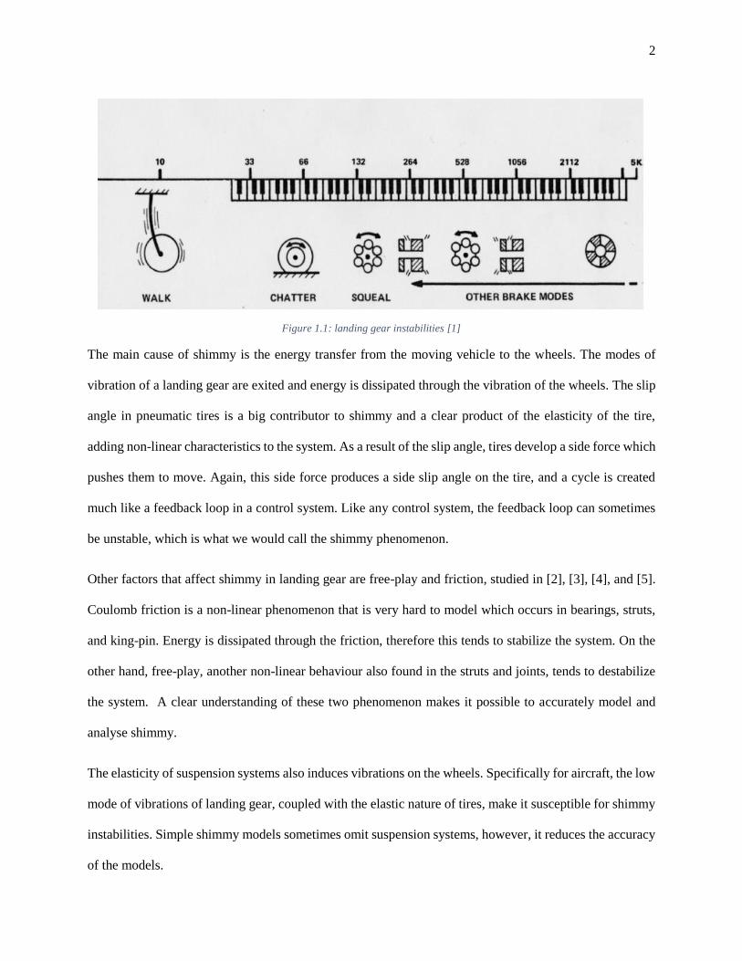
2

Figure 1.1: landing gear instabilities [1]

The main cause of shimmy is the energy transfer from the moving vehicle to the wheels. The modes of

vibration of a landing gear are exited and energy is dissipated through the vibration of the wheels. The slip

angle in pneumatic tires is a big contributor to shimmy and a clear product of the elasticity of the tire,

adding non-linear characteristics to the system. As a result of the slip angle, tires develop a side force which

pushes them to move. Again, this side force produces a side slip angle on the tire, and a cycle is created

much like a feedback loop in a control system. Like any control system, the feedback loop can sometimes

be unstable, which is what we would call the shimmy phenomenon.

Other factors that affect shimmy in landing gear are free-play and friction, studied in [2], [3], [4], and [5].

Coulomb friction is a non-linear phenomenon that is very hard to model which occurs in bearings, struts,

and king-pin. Energy is dissipated through the friction, therefore this tends to stabilize the system. On the

other hand, free-play, another non-linear behaviour also found in the struts and joints, tends to destabilize

the system. A clear understanding of these two phenomenon makes it possible to accurately model and

analyse shimmy.

The elasticity of suspension systems also induces vibrations on the wheels. Specifically for aircraft, the low

mode of vibrations of landing gear, coupled with the elastic nature of tires, make it susceptible for shimmy

instabilities. Simple shimmy models sometimes omit suspension systems, however, it reduces the accuracy

of the models.

3

1.2 Landing gear mechanical models

Landing gears are complicated systems that need to be simplified in order to obtain reasonable dynamic

models that can be solved. Different ways of simplifying these systems have been implemented over the

years focusing on the interaction between the wheel and the ground. The following three mechanical models

are widely used in shimmy analysis and are named depending on the number of coefficients in their

characteristic equation.

1.2.1 Third-order model: simple trailing wheel system with yaw DOF

The third-order system has only one degree of freedom, the yaw angle, and assumes a massless tire that

rotates laterally about a pivot point with some stiffness and damping, much like a caster wheel, with a caster

length of 𝑒 (See Figure 1.2). The straight tangent tire model is used in [6] and [7], along with the Routh-

Hurwitz criterion, to plot the stability regions of the system depending on the velocity, caster length,

damping, and stiffness. A more in depth look at tire models and stability criterions are shown in Chapters

2 and 3 of this thesis.

Figure 1.2: simple trailing wheel system [6]

1.2.2 Fifth-order model: yaw and lateral DOF

The fifth-order system is similar to the third-order one but with added lateral flexibility which models the

flexibility of a cantilevered gear, see Figure 1.3. This increases the DOF to 2, the yaw rotation of the tire

and the lateral deflection, which increases the order of the characteristic equation to five. The differential

4

equations become more complex and more terms are taken into account when analysing for stability. Again,

the straight tangent tire model has been used in [8] to study shimmy in this system.

Figure 1.3: trailing wheel system with lateral compliance [6]

It can be noted that a third-order system can be obtained if the tire is assumed to be rigid for the fifth-order

system with lateral compliance. Shimmy is also seen in this system showing that there are different causes

for tire instabilities, not only their elastic nature.

1.2.3 Seventh-order model: fifth-order system with steering

The most realistic model of the three presented in this section is the seventh-order system which accounts

for a steerable system added to the fifth-order model. Once again, the straight tangent model has been used

in [6] to analyse and plot the stability regions of a seventh-order system.

Higher order models can be obtained by adding more degrees of freedom. This increases the complexity of

the models which makes them extremely difficult to solve.

1.3 Vehicle dynamics

To fully understand and study the shimmy phenomenon, the vehicle dynamics, in this case the tire

dynamics, must be understood to be able to create a mathematical description of the landing gear. Landing

gears have tires, just as automobiles, the only difference is the configuration of these tires and whether or

5

not they steer. So, in terms of the vehicle dynamics, tires generate some forces and moments depending on

some input parameters. These input parameters are the tire slips, and the tire normal force 𝐹𝑧. The tire

outputs are the remaining forces and moments. These forces, along with the tire slip 𝛼 angle can be seen in

Figure 1.4.

Figure 1.4: Tire moment and forces [6]

1.3.1 Tire slips and angles

The tire’s elasticity makes it bend in all directions due to inertial and other external forces. Due to this

elasticity, only a portion of the tire, called the contact patch, directly touches the ground, creating what is

called an effective radius 𝑟𝑒. The point 𝑆 is located at this 𝑟𝑒 away from the center. The effective radius is a

function of the amount of vertical deflection 𝜌, called radial deflection, experienced by the tire due to a

vertical load. This quantity, along with the velocities of the tire at different points, such as the velocity of

the tire in the longitudinal direction 𝑉𝑥, and the velocity of the tire at point 𝑆 called 𝑉𝑠𝑥, are shown in Figure

1.5. The different types of tire slips are: longitudinal slip 𝜅, lateral slip 𝛼, and spin slip 𝜑. The camber angle

𝛾, also called the inclination angle, is also an input to the tire.

6

Figure 1.5: effective radius and tire velocities [6]

The longitudinal slip is the ratio between the longitudinal slip velocity at point S of the tire, and the forward

speed of the tire itself. This ratio shows how much traction the tire has, as well as if it is driving or braking.

The formula is

𝜅 = −

𝑉𝑠𝑥𝑉𝑥

(1-1)

The slip angle of a tire defines the ratio between the lateral velocity and the longitudinal velocity. It is

basically the angle at which the wheel is pointing at with respect to its actual displacement direction. The

formula is

𝑡𝑎𝑛 𝛼 = −

𝑉𝑦

𝑉𝑥 . (1-2)

The spin slip defines the amount of slip produced due to steering. When a wheel steers, there is some friction

in the contact patch of the tire as it has to turn with a certain area of the tire touching the ground. The

formula for the spin slip is

𝜑 = −𝜔𝑧

𝑉𝑐 , (1-3)

where 𝜔𝑧 is the speed of the wheel body along a normal to the road plane 𝑛 [6], see Figure 1.6.

7

Figure 1.6: tire coordinte axis with angular and translational velocities [6]

The camber angle, or the inclination angle, usually denoted by 𝛾, is a measure of the angle between the

wheel center plane and the normal to the road 𝑛, see Figure 1.6. For the purpose of this thesis, the camber

angle will always be assumed to be zero, as it is usually the case for landing gear tires.

1.3.2 Tire forces and moments

Due to the different tire slips that are developed, different types of forces and moments are created in the

tires. In general, two forces and three moments are created: the longitudinal force 𝐹𝑥, the lateral force 𝐹𝑦,

the overturning moment 𝑀𝑥, the self-aligning moment 𝑀𝑧, and the rolling resistance moment 𝑀𝑦. A force

in the 𝑧 direction is not developed by the tire, but rather is an input to the tire, and comes from the weight

of the aircraft itself.

The longitudinal force is produced due to the longitudinal slip and is responsible for the longitudinal motion

of the vehicle. Thus, this force can be a driving or a braking force. The lateral force is produced due to the

slip angle and is responsible for pushing the vehicles to the sides allowing them to turn.

The self-aligning moment is also produced due to the slip angle of tires and also due to the lateral force.

The pneumatic trail, which is the distance at which the lateral force acts away from the center of the tire,

8

induces the self-aligning moment. Tire friction also affects the self-aligning moment. The overturning

moment is produced by the elastic nature of the tire which deforms due to the lateral force. A moment in

the 𝑥-axis is created due to the position of the normal force with respect to the wheel plane, or tire point of

rotation about the 𝑥-axis. The rolling resistance moment is created by the hysteresis in the tire tread and

also due to friction between the tire and the road, which prevents the tire from spinning in the 𝑦 axis, and

thus creating a moment. Speed is also a factor that contributes to rolling resistance [9].

1.4 Tire models

There has been several tire models developed over the past 50 years or more. These models are produced

through different methods with one common goal: to obtain a mathematical representation of the dynamics

of tires. As it was shown before, tires develop different forces and moments due to their interaction with

the ground. Using Pacejka’s [6] background information regarding tire modeling in Figure 1.7, we can see

the different types of models that can be obtained. The main types of models are either theoretical or

empirical. Newer models rely on computer software to discretize the tires into very small pieces to increase

the accuracy.

9

Figure 1.7: different types of tire models [6]

The most empirical tire model is the magic formula tire model which is based in trigonometric functions

that describe the tire forces and moments depending on different parameters. More physical models, like

the brush tire model or the string tire model, use physical representations of the tire to develop

mathematical descriptions for their dynamics behaviour. Finally, the more theoretical tire models usually

use FEM like theories and discretize the tires into small pieces, such as the FTire model.

1.4.1 Analytical tire models

The long history of tire models is summarized to understand their evolution and their applications for

shimmy analysis. One of the first researchers to study the shimmy phenomenon in aircraft was Dietrich

(1941) using the model of a stretched string developed by Von Schlippe (1941) in the same paper. Later

on, Dietrich (1943) studied the effect of the tire treads on shimmy. Segel (1966) obtained the frequency

response functions for the one-dimensional Von Schlippe string model, which further helped the study of

shimmy. After many researchers had come up with their own tire models and shimmy analysis, Smiley

10

(1956) presented a linearized tire motion, similar to that of Von Schlippe, which summarized many of the

existing theories at the time. One of the first people to study the non-linear dynamics of the tire with respect

to shimmy was Pacejka (1966) in [8], developing a straight tangent approximation to Von Schlippe’s string

theory. Over time, many other researchers used Von Schlippe’s string theory, or a modification of it, to

analyse and study shimmy.

Von Schlippe’s string theory was based on the idea of a finite length string with a definite contact area that

touched the ground. Another type of tire model developed by Keldysh (1945) and Moreland (1954) was

called the point contact tire model because the contact area was reduced to a single point; in other words it

was equal to zero. The contact point is held in place by a spring which represent the stiffness of the tire.

Both models are very similar with some small discrepancies, one of them being that Moreland came up

with a time lag term to account for the tire’s retardation effects.

The analysis of shimmy on a simplified nose landing gear was done by Somieski (1997) in [10] using the

elastic string theory to model the tire. Linear and nonlinear mathematical methods were used to study

shimmy in a single caster wheel. The calculation of the eigenvalues and numerical simulation of time

histories, and solving for the stability boundaries with a parameter space model are just some of the methods

used in this paper to obtain the stability regions of the system regarding shimmy. This simple model is a

good guideline for landing gear stability and shimmy analysis.

Due to the complexity of landing gear systems, it is sometimes hard to develop accurate analytical models

for shimmying wheels. It is of common practice to simplify the moving vehicle as much as possible, and to

focus on the parts that interact with the wheel itself. Some parts in a model can be assumed to be rigid,

while others are assumed to be elastic. Stepan (1991) studied the chaotic motion of wheels in [11] using a

single towed tire, applying Coulomb friction for the wheel-ground interaction, and assuming rigid wheels;

thus, there was no need to use a tire model. Since Von Schlippe started studying shimmy, he realized that

pneumatic tires have a delay effect. The contact area of tires have some sort of memory and behave

11

accordingly depending on where they have been before. Stepan (1998) studied this delay in pneumatic tires

along with the shimmy phenomenon and chaos in [12]. The delay effects of tires and their relation to

shimmy were studied more in depth in [13] using the stretched string model.

Having models with different approaches makes it hard to know which one can be used more appropriately

for shimmy analysis. The paper [3] makes a complete summary of the research and development of every

part that makes a landing gear for simulation purposes. The conclusions obtained from these authors

regarding all the previous research were that the most common model for shimmy analysis is Von

Schlippe’s stretched string, while Pacejka’s straight tangent and Smiley’s model are less often used in this

field.

Lately, Besselink (2000) studied the shimmy phenomenon in landing gear in [7], summarizing the findings

of every past researcher regarding tire modelling and their application to shimmy. The stretched string

models and the point contact models were compared, along with their respective transfer functions, to see

which one could be used more appropriately for shimmy analysis.

More recent models using dry friction to study the interaction between the wheel and the ground for rigid

tires can be found in [14]. This research is an example of how friction is also a cause of shimmy, even

though the tires are assumed to be rigid. Without using an elastic tire model, the authors were able to

demonstrate analytically and experimentally that dry friction alone between the wheel and the ground

causes instabilities.

Recent research comparing tire models using a constant and a non-constant relaxation length was presented

in [15]. Through the use of different mathematical techniques such as energy flow diagrams, bifurcations,

and the Routh-Hurwitz criterion, along with the use of the magic formula model, and including the structural

damping, the authors were able to conclude that the non-constant relaxation length does affect shimmy

analysis at large amplitudes of vibration and must definitely be included for more accurate models.

12

1.4.2 Numerical tire models

Newer numerical tire models have been recently developed which take advantage of the fast processing

power of computers nowadays. Some common ones are the Fiala, UA, TRR64, PAC, and FTire model.

Most of these models are based on analytical models but are implemented in a multibody dynamic software

environment due to their complex mathematical equations that are usually extremely hard to solve

analytically. Some of these models are strictly physical representations of the tire, such as the Fiala, UA,

and TRR64 mode. They either model the tire as a beam, a disc, or any other physical shape with different

types of stiffnesses. The PAC model is a more empirical model which is developed by performing a number

of experiments to figure out different coefficients and parameters for the formulas that describe the tire’s

forces and moments. Finally, the more sophisticated FTire model is a FEM-like model which discretizes

the tire into a finite number of belt elements which make a flexible ring figure. All these models can be

found in the multibody software MSC Adams.

1.5 Shimmy modelling

Analytical models can only go so far in analysing shimmy in landing gears. As it was previously explained,

many simplifications are made to be able to work with a model that can be solved. A numerical approach

is sometimes sought to incorporate complexities into the systems. Multibody dynamics software are

commonly used in the area of vehicle dynamics to analyse for vehicle stability, handling, steering, brakes,

and controls. These types of software can be used to study the shimmy phenomenon in landing gear using

a well-built tire model.

There are some examples of research that studied shimmy in landing gears using MSC Adams in [16], and

using SIMPACK in [1], [17], and [18]. The common technique in these studies is to test different tire models

and compare them with experimental results. Then, through a parametric approach, the parameters of the

system that affect shimmy are found.

13

The figure below shows how a landing gear is modelled using a multibody dynamics software. Basically,

the main bodies such as the tires, main struts and piston, and torque links are chosen and connected to each

other through links or joints. Tire models are then used to determine the forces that act on the wheels

depending on input parameters such as road conditions, friction coefficients, and tire characteristics.

Figure 1.8: multi-body model of a landing gear [17]

1.6 Control and stability analysis

The control of shimmy is an important aspect of the design of landing gears. Different control theories and

stability criterion are used to analyse and manipulate the stability of these systems. Depending on

parameters such as the stiffness, damping, and geometry, the system can become unstable. Stability regions

are usually plotted to have a clear and visual understanding of how these parameters affect the shimmy

vibrations.

For linear dynamic systems, the eigenvalues can be calculated to check for stability around nominal

conditions. The roots of the characteristic equation of the system yield the eigenvalues. If any eigenvalue

14

has a positive real part, then the system response will be unstable. A positive real root means that the system

will drive away from steady state, a negative real root means the system will drive back to steady state, and

an imaginary root means the system will oscillate; a combination of these responses is possible. Plotting

the eigenvalues in a plane with parameters of importance, such as velocity and caster length, can give some

insight into which parameters will make the system unstable. The paper [10] used the eigenvalues of the

linearized model of a single caster wheel to check for instabilities depending on the velocity of the vehicle

and its caster length.

The Routh-Hurwitz criterion is another method of analysing the stability of a dynamic system. The criterion

states that each coefficient of the characteristic equation of the system and each Hurwitz determinant must

be greater than zero to obtain stability. A more in depth look at the criterion can be found in the literature

[19].

The use of this criterion is common in shimmy analysis. The stability analysis of a trailing wheel model

was performed in [7] using the Routh-Hurwitz criterion yielding inequalities which can be plotted to obtain

stability boundary regions. In the latter work, parameters such as the velocity of the vehicle, caster length,

stiffness, and damping were used in the plots to check for instabilities.

This method is also heavily used in [8] and [6] to explore the stability of third order systems, which are

simple and linear; fifth order systems, which have one more lateral DOF at the king pin; and the seventh

order system, which is a more realistic model incorporating a steering DOF.

A popular method for solving the non-linear differential equations of the tires and the shimmy phenomenon

is called the feedback linearization technique. This method transforms a set of non-linear coordinates into

one that is linear and controllable. Feedback linearization is commonly applied to the classic shimmying

wheel model, as shown in [20], to linearize the strong nonlinear differential equations of motion into a set

of linear equations that can be solved.

15

Bifurcation curves are typically used to determine the stability regions of a landing gear depending on

multiple parameters. Usually, the bifurcations are plotted on a plane having two important parameters, such

as the velocity of the vehicle and the normal force on the tire, and then other parameters like stiffness and

damping are changed to check for stability. The use of the Hopf bifurcation curves can be seen in [21] to

check the influence of the wheel separation distance and the moment of inertia of the wheels in a landing

gear on stability. Bifurcation curves were also used, by the same authors, in [22], to analyse the interaction

between the lateral bending mode and the torsional mode of vibration in a landing gear, which are coupled

by the nonlinear elastic forces of the tires.

It is very common to apply control theory to the tire instability problem. The system is treated as a closed-

loop system with feedback. The system is separated in two: the landing gear structure and the tire (see figure

below for the control scheme of the trailing wheel model). The slip angle in the tire creates a side force,

which in turn, create a side slip. This closed-loop system can be represented by a transfer function which

can be used to analyse for stability (see figure below for a feedback loop control representation of the

shimmy problem). It is also very common to transform the model into state space.

Figure 1.9: Closed-loop feedback model of the trailing wheel model [7]

Apart from the methods shown before, there are other tools used to analyse shimmy and the stability of

landing gears. For instance, Bode plots can be used to evaluate shimmy in the frequency domain,

determining at which frequency shimmy occurs more aggressively. The Nyquist criterion and root locus

can be used to explore the stability of a system in state space given their transfer function.

16

More advanced control systems with fuzzy logic are been used to control the shimmy vibrations in landing

gears. In the paper [23] the dynamic model of a nose landing gear is used for active shimmy damping where

the system is transformed in state space, and adaptive control theory is used to account for the constant

change in tire characteristics. A stability analysis is performed and the controller successfully avoids

shimmy vibrations in nose landing gears.

1.7 Shimmy dampers

To reduce the amount of vibrations and instabilities in a landing gear due to shimmy, one of the possible

solutions is to introduce a damper into the system. A shimmy damper is often placed at the torque link apex

between the upper and lower torque links (see Figure 1.10).

Figure 1.10: Components of a cantilevered landing gear [7]

One of the few drawbacks with dampers is that they add weight and maintenance costs. On the other hand,

they reduces shimmy vibrations significantly preventing any accidents. The successful implementation of

a shimmy damper on a twin cantilevered gear of a Fokker F28 is shown in [24]. In this research paper, the

Lagrange equation was used to obtain the equations of motion of the system, taking into account the

17

gyroscopic effects of the tires, for the landing gear with and without the damper. The model was validated,

and the damper was tuned for maximum efficiency. The results proved to reduce the amount of instabilities

significantly. Another analytical study of the effects of a shimmy damper in a landing gear were performed

in [25] calculating the stability regions of the system.

1.7.1 Types of shimmy dampers

There are different types of shimmy dampers that work for nose or main landing gear. These are classified

depending on the type of damping element used. Some of the most common shimmy dampers in the

industry today are: hydraulic damper, magnetorheological damper, steering mechanism as shimmy

damper, solid media damper, and friction damper.

Hydraulic shimmy dampers use a hydraulic system, usually a dashpot type, where fluid passes through a

small opening to dissipate kinetic energy. Rotary or linear dampers are used depending on the applications

and position. For steerable nose landing gears, hydraulic steering systems are usually used as dampers when

landing or taking off.

For the magnetorheological dampers, active control systems are used in hydraulic dampers to eliminate

shimmy vibrations. A special fluid containing ferromagnetic particles makes it possible for a control system

to change the viscosity of the fluid depending on the applied magnetic field.

Some nose landing gear wheels use their hydraulic steering system as a shimmy damper when landing and

taking off. During these activities, steering is seldom used, so, the fluids inside of the pistons are used to

prevent vibrations travelling from the landing gear piston to the landing gear upper strut.

Elastomers have also been used as dampers due to their mechanical properties, these dampers are also called

solid media dampers. Lighter than hydraulic systems, elastomer dampers are placed inside linear pistons,

replacing the fluid and orifice, where tension or compression happens when the landing gear piston tries to

rotate relative to the landing gear strut. Energy is dissipated in the form of heat as the elastomer expands or

compresses.

18

Friction dampers are lighter systems that do not rely on the use of hydraulics to dissipate the vibration

energy from landing gears. Friction pads are biased against one another, normally in a rotary fashion, to

create friction and dissipate the kinetic energy between the piston and the strut. Friction between the landing

gear struts is usually sought and not prevented as it helps reduce shimmy vibrations.

1.7.2 Shimmy damper patents: steerable vs. non-steerable wheels

There are many shimmy damper patents to date. Different types of dampers have been used in different

configurations. Rotary hydraulic shimmy dampers placed at the main shock struts that work with the

steering mechanism of nose landing gears can be seen in [26] and [27]. A rotary damper was also used in a

twin-tire landing gear in [28] and [29] where both wheels are allowed to move freely during normal

operation but are attached together through the damper while shimmying to reduce instabilities. Twin-tire

landing gears are known to shimmy frequently, and a common solution is to rigidly fix the tires together.

The latter invention provides for a solution that helps reduce these vibrations, while improving on tire wear

and other areas. A fluid control steering system used along a linear damper attached to the main strut by

means of a rack is shown in [30]. A set of two linear hydraulic dampers, each with a fluid reservoir, are

placed in series on either side of the main strut of a nose landing gear in [31], see Figure 1.11. A linear

dashpot is used in [32] to reduce the shimmy vibrations of a steerable landing gear wheel.

19

Figure 1.11: linear shimmy damper for nose landing gear [31]

A shimmy damper made of an elastomer material is presented in [33] and [34]. The advantages of not using

a hydraulic damper are the reduction of weight and removal of possible leakage. Maintenance is also easier

and less expensive. Elastomer dampers can be compressed, expanded, or twisted, dissipating energy.

Different set-ups of this type of damper can be found, but they all have the same goal. Another type of non-

hydraulic shimmy damper which does not interfere with the existing landing gear design and steering

system is presented in [35]. The damping is provided by a rotary friction pad biased against a fixed member

which resists rotation and dissipates energy.

Newer patents regarding shimmy dampers propose the use of active control systems to mitigate instabilities.

Successful implementation of this system in automobiles is proposed in [36] using sensors that check for

shimmy oscillations and control the brakes to eliminate such instabilities. A similar approach could be used

for aircraft landing gear with some small modifications.

A cavitation-free hydraulic shimmy damper that is not sensitive to oil temperature changes is proposed in

[37]. This invention uses a hydraulic compensator with a big internal fluid volume and a manifold placed

20

between the damper and said compensator. The internal fluid volume of the compensator helps to minimize

the effects of the drastic temperature changes due to shimmy vibrations.

The most used shimmy dampers today are the ones that are placed at the torque links of the landing gear.

A well-known patent developed by Boeing in [38], see Figure 1.12, presents a linear damper placed between

the upper and lower torque link that prevents translational vibrations between them. A fluid reservoir and

a set of Belleville springs are used to improve performance and add a stiffness and dampening force.

Figure 1.12: Boeing shimmy damper [38]

A newer version of this type of damper, developed by UTC Aerospace Systems in [39], see Figure 1.13,

replaces the upper torque link with a two arm system: one arm a cantilevered beam, and another arm a

damping device which could be made of any type of damping system available. Translational motion

between the torque links bends the beam, which acts as a spring, and also compresses or extends the

damping device. These dampers are not restricted to a certain degree of rotation because they are connected

to the torque links. They can also be installed in any landing gear even after they have been designed and

manufactured.

21

Figure 1.13: UTC Aerospace Systems shimmy damper [39]

1.8 Shimmy prevention and solutions

Many researchers have pondered on the idea of creating a simple and perfect solution for shimmy. As it

can be noted, it is merely impossible to eliminate wheel instabilities completely. Landing gears are complex

systems with many parameters, nonlinearities, free-play, and worn materials. Suggestions are usually made

through stability analyses to prevent shimmy at high speeds as it can be catastrophic.

For instance, reference [7] explains there are mainly two areas of stability derived from the trailing wheel

system with lateral flexibility: a small negative trail with low yaw stiffness and high lateral stiffness, and

large positive trail with a high yaw stiffness and low lateral stiffness.

Other general practices to diminish wheel shimmy vibrations in landing gears are to increase the torsional

stiffness of the structure, use an appropriate pneumatic trail given by a stability analysis, the use of co-

rotating wheels, to incline the landing gear structure, and use friction and hydraulic damping to dissipate

energy [40].

22

1.9 Thesis outline and research objectives

This thesis studies the shimmy phenomenon, but more in-depth, it studies the solutions that can be applied

to prevent these vibrations. The most common solution is the shimmy damper, thus this work focuses on

shimmy dampers, their dynamic response, and the parameters that affect the stability of the system.

In Chapter 2, a clear and in-depth explanation of the different tire models that can be used to study shimmy

are presented. The tire models used in multibody software and those used for analytical methods are

presented in this section.

The analytical approach to study shimmy, and the methodology to analyse the stability of the system is

presented in Chapter 3. Using the differential equations of motion of a landing gear and shimmy dampers,

along with tire models, the stability of landing gears can be determined depending on certain parameters.

The use of a multibody dynamics model developed in MSC Adams is shown in Chapter 4 of this thesis.

The same parameters from Chapter 3 are used, however, the dynamics are computed by the software and

the dynamic response is shown for different configurations. Finally, some discussions and conclusions are

given in Chapter 5. Shimmy damper design recommendations are also given regarding the design of a

shimmy damper and the lessons learned during this research.

The main objective of this work is to study the stability and dynamic response of different shimmy dampers.

Most research papers use the rotational stiffness and damping coefficient of landing gears whilst studying

stability, while in reality part of the stiffness and damping comes from a translational spring and damper,

the shimmy damper. The proper implementation of a shimmy damper and how it affects the dynamic

response of the system is mostly inexistent in current research, so this thesis will explore the effects of the

parameters of real shimmy dampers in non-steerable landing gears. The specific shimmy dampers from

Boeing [38] and UTC Aerospace Systems (UTAS) [39] will be the focus of this thesis. Furthermore, a

dynamic model of a landing gear will be developed and validated to be able to study the dynamic response

of different types of shimmy dampers, and the effect their parameters have on stability. The dynamic

23

response of the different shimmy dampers can give us an insight into their performance and effectiveness

at mitigating shimmy vibrations. Finally, a new and improved damper will be proposed using the tools

developed in this thesis, such as the stability analysis and the landing gear model. The new design will focus

on reducing the overall weight, cost, maintenance, and increasing the ease of manufacturability and

installation. The aim is to design a new type of shimmy damper that is more efficient at mitigating the

vibrations than other dampers found in the industry today.

24

Chapter 2 Tire modeling for shimmy analysis

To further study the shimmy phenomenon and the dynamic response of different shimmy dampers, a robust

tire model that can be used in a multibody software is needed. Tire models are mathematical representations

of tires that describe their dynamic behaviour depending on certain parameters. Being able to use the

differential equations that describe the motion of tires, not only in an analytical approach, but also in a

numerical software scheme, is of great importance. The following section shows a more in-depth look at

the types of tire models found in the multibody software MSC Adams and how they work. Then, analytical

tire models are shown how they are implemented in a multibody software. The stretched string model,

which can be incorporated into the multibody software MSC Adams, is presented as part of the tire’s

analytical models.

2.1 Numerical tire models

The tire models used in the multibody software MSC Adams are all numerical models which approximate

the behaviour of tires through different methods and physical representations. The literature review of this

thesis gave a small introduction into the different types of tire models. The following section will go further

in explaining these models. The main models studied are: Fiala, UA, PAC2002, Aircraft, and FTire, and

can be divided in three categories. The first category is comprised of the Fiala, UA, and the Aircraft models.

These all use the same tire forces and moments descriptions with different degrees of complexity and

25

degrees of freedom. The PAC tire model is in the second category, a unique model which uses Pacejka’s

magic formula [6]. These formulas approximate the nonlinear tire forces and moments using trigonometric

functions. Finally, the FTire model is in the third category with the FEM-like models.

2.1.1 Fiala

The Fiala tire model is a physical representation of the tire and its properties. It models the tire as a beam

on an elastic foundation in the lateral direction. The contact between the beam and the road is denoted by

elastic brush elements. The longitudinal and lateral forces that are developed on the tire are obtained through

the steady-state slip characteristics [41]. Some assumptions made are that the contact patch is rectangular,

and that the camber angle has no effect on the tire forces.

As per any Adams tire model, one of the inputs of the Fiala tire model is the “.tir” tire property file. This

file contains all the parameters needed to fully define the tire such as the radius, stiffness and damping

coefficients, etc. The second input to this tire model is the tire’s kinematics states such as the longitudinal

slip and slip angle. In the appendix section, in Table 0.2, we see the inputs given to this tire model obtained

from the Adams documentation [41]. The rest of the input parameters are, as mentioned before, the slip

angle, longitudinal slip, and tire’s deflection, which are all calculated by Adams’ solver. The remaining

ones, like the tire’s mass and radius, are input by the user.

The two type of slips found in this model are: longitudinal and lateral. The lateral slip is also called the

slip angle. The longitudinal slip 𝜅 (also denoted as 𝑆𝑠), and the slip angle 𝛼 are defined using

conventional vehicle dynamics terminology. Then, a combined, or so called comprehensive slip 𝑆𝑠𝛼 is

computed which takes into account both the longitudinal and lateral slip. The friction coefficient is

computed as a linear quantity between the maximum and minimum ranges specified by the user in the

inputs, see Table 0.2.

The tire forces and moments are then calculated using the quantities computed before: the comprehensive

slip, the longitudinal slip, the lateral slip, the friction coefficient, and other user inputs. The normal force

26

is a simple addition of the forces created by the vertical stiffness and damping of the tire, created due to

the tire’s vertical deflection. The longitudinal force is calculated using the longitudinal slip 𝑆𝑠, the input

CSLIP, the coefficient of friction, and the tire’s normal force. Similarly, the tire’s lateral force is

calculated using the slip angle, the friction coefficient, the input CALPHA, and the tire’s normal force.

The rolling resistance moment is calculated using a constant and the tire normal force, while the tire’s

self-aligning moment is calculated using the tire’s side force.

2.1.2 UA

The UA tire model is a more in depth and complicated model than the Fiala tire model. It also models the

tire as a disk with a single contact point at the ground. The main difference is that UA tire model has both

longitudinal and lateral relaxation effects.

The inputs of the UA tire model are all the kinematic states of the tire, as well as the “.tir” file with the

remaining tire parameters such as the tire’s radius, stiffness, damping, etc. The

Table 0.3 seen in the appendix, obtained from Adams documentation [41], summarizes the inputs of the

UA tire model which are thoroughly explained in [42]. The tire slip quantities are defined exactly the same

as in the Fiala tire model, using conventional vehicle dynamics terminology. The slip ratios are also the

same as in the Fiala tire model, except for the addition of the lateral slip ratio due to camber 𝑆𝛾. A combined

lateral slip ratio, 𝑆𝛼𝛾, is computed using the slip angle and the lateral slip ratio due to camber. Finally, a

resultant slip ratio, 𝑆𝑠𝛼𝛾, is computed using all three slip ratios.

The tire forces, such as the normal, longitudinal, and lateral, are all calculated just like in the Fiala tire

model, except now there is a resultant slip ratio which takes into account the camber angle. The same is

done for the tire moments. However, because camber angle is taking into account, the expression for some

of the tire forces and moments are more complicated and depend on the different tire states and dynamics.

27

2.1.3 Aircraft tire models

There are three different aircraft tire models to be used in Adams. These are: Aircraft basic, Aircraft

enhanced, and Aircraft TRR64. The first two are based on the Fiala tire model, while the latter one is made

from a different formulation shown in [43]. The Aircraft tire models are made specially for landing gears

because these models take into account, for instance, higher tire pressures, different load-deflection curves,

and higher maximum tire vertical forces 𝐹𝑧. Apart from these, there is really no basic difference between

these Aircraft tire models and the ones shown before in terms of handling forces, tire slips, inputs and

outputs.

Aircraft basic

This tire model is heavily based on the Fiala tire model shown before. The tire is represented by a disk

which touches the ground on a single point. It is assumed that there are no lateral, longitudinal, and twist

deformations effects on the tire center moments [41]. The inputs and output of the Aircraft basic tire model

are exactly the same as those in the Fiala one. The tire slips and tire forces are expressed just as it is done

in the Fiala tire model.

Aircraft enhanced

The Aircraft enhanced tire model uses either the Fiala or the UA tire model. The user can choose which

handling method to use, thus all the tire slips, inputs and outputs, and tire forces are expressed the same

way as in whichever method the user chooses. It is enhanced because the user can choose to use the

enhanced UA tire model which does a better job at describing tires and their dynamic properties.

Aircraft TRR64

This tire model was developed by NASA in [43] and is somwhat different from the ones previously shown.

The TRR64 also models the tire as a single disk which touches the ground at one point. The tire’s kinematic

states are calculated differently, but the handling forces can be calculated using either the Fiala or the UA

tire model.

28

The table shown in the appendix, Table 0.4, summarizes the inputs for the Aircraft TRR64 model, some

of which are similar to those previously discussed before in this report. Using these inputs a few terms are

developed which are then used to express the tire’s kinematic states, and later, the tire forces. We start

with the tire’s physical dimensions, such as the unloaded diameter D0, which is then used to calculate the

longitudinal stiffness of the tire 𝐾𝑙𝑜𝑛 and the lateral stiffness of the tire 𝐾𝑙𝑎𝑡, which also takes into account

the inflation pressure. The tilt/camber stiffness 𝐾𝑔 is computed using the normal force of the tire. The

tire’s slip stiffnesses, CSLIP, CALPHA, and CGAMMA, which are the tire’s longitudinal, lateral, and

camber slip stiffnesses respectively, are calculated using the previously computed 𝐾𝑙𝑜𝑛, 𝐾𝑙𝑎𝑡, 𝐾𝑔.

The tire forces are developed depending on the type of handling force method chosen by the user. Either

the Fiala or the UA tire model can be chosen, and thus, the longitudinal and lateral tire forces will be

developed just as it was shown for the respective tire models. The only difference in the TRR64 tire model

is on the tire kinematic states which are express differently using the tire’s physical states and are not

expressed by the user.

2.1.4 PAC2002

The PAC2002 tire model is heavily based on the tire model developed by Pacejka, which calculates the

forces and moments with the famous magic formula tire model [6]. In comparison with the previously

discussed models, which have been a physical approximation of the tires by using a disk with a single

contact point, or a string with some specific features, the PAC2002 model is an empirical model based on

trigonometric functions that predict the forces and moments on the tire depending on the tire’s kinematic

states, given some parameters. These parameters define the trigonometric function’s shape, and are found

through experimentation.

These trigonometric functions are the basis of the model and they describe a certain output 𝑌, given a certain

input 𝑥. The following two functions are the basis for the magic formula tire model [6]:

29

𝑌(𝑥) = 𝐷 𝑠𝑖𝑛[𝐶 𝑎𝑟𝑐𝑡𝑎𝑛{𝐵𝑥 − 𝐸(𝐵𝑥 − 𝑎𝑟𝑐𝑡𝑎𝑛(𝐵𝑥))} ] (2-1)

Where 𝑌(𝑥) could be the longitudinal force 𝐹𝑥, and 𝑥 the longitudinal slip 𝜅, or 𝑌(𝑥) could be the lateral

force 𝐹𝑦 and 𝑥 the lateral slip 𝛼.

𝑌(𝑥) = 𝐷 𝑐𝑜𝑠[𝐶 𝑎𝑟𝑐𝑡𝑎𝑛{𝐵𝑥 − 𝐸(𝐵𝑥 − 𝑎𝑟𝑐𝑡𝑎𝑛(𝐵𝑥))}] (2-2)

Where 𝑌(𝑥) could be the pneumatic trail 𝑡 and 𝑥 the slip angle 𝛼. The self-aligning moment is a function

of the pneumatic trail and the side force 𝐹𝑦, thus, it could be calculated using these two equations. Each of

the parameters used in the equations shown above change the shape of the function.

The amount of inputs used for the PAC2002 is enormous, and this is because of the nature of the magic

formula. The inputs can be divided into the kinematic states, and the tire parameters. On the other hand, the

outputs of the model are the longitudinal and lateral fore, and the three moments created by the tire:

overturning moment 𝑀𝑥, rolling resistance moment 𝑀𝑦, and self-aligning moment 𝑀𝑧.

Tire parameters are given to modify the shape of the trigonometric functions. There are around one hundred

parameters, and these serve to modify or scale different aspects of the tire’s behaviour. These are called

scaling factor coefficients, and they can be found for pure slip, combined slip, and transient response

conditions. There are scaling factors for: longitudinal force at pure and combined slip, lateral force at pure

and combined slip, self-aligning moment at pure and combined slip, turn-sip and parking parameters, and

rolling resistance at pure and combined slip. Other scaling factors are used for transient handling modes,

which take into account the changes on the inputs due to time. All these parameters are usually obtained

experimentally or through the manufacturer. Thus, we can see how complicated the PAC2002 model can

be, and how different it is from the previously explained UA and Fiala tire models.

The tire slips for this tire model are basically the same ones used before for the UA and Fiala tire model.

The same definitions are used to define the longitudinal and lateral slip. However, a new slip is introduced

in this model, the turn slip 𝜑, and it is defined using the tire’s yaw velocity [41].

30

Using the expression previously shown as the magic formula, we can develop the tire forces as per the

PAC2002 tire model [6]. The longitudinal force is a function of the longitudinal tire slip. The first

expression, Eq. (2-1), is used to express 𝐹𝑥. The lateral force is a function of the slip angle, and it is

expressed using Eq. (2-1) as well. The aligning moment is obtained indirectly through the magic formula.

The self-aligning moment is a function of the side force and the pneumatic trail of tire 𝑡, which is the

distance at which the side force 𝐹𝑦 acts from the center of the tire. The pneumatic trail can be calculated

using the Eq. (2-2).

2.1.5 FTire

The flexible ring tire model is a more complicated and sophisticated model used for vehicle dynamics

simulations and vehicle ride comfort analysis. This is a highly non-linear model that can be used in the

domain of up to frequencies of 120 Hz, and can deal with many nonlinearities such as: potholes, cleats, and

single obstacles. This model runs fairly fast compared to other tire models as it doesn’t need any

complicated road data processing.

The tire belt is represented as a flexible ring with bending stiffness, elastically connected to the rim with

springs in the radial, tangential, and lateral directions. The ring is composed of a finite number of masses

that are coupled with each other by stiff springs in both in-plane and out-of-plane directions. The FTire

model calculates all the bending stiffnesses and damping factors during pre-processing, and then it

calculates all six components of the tire forces and moments acting on the rim.

Due to a lack of experiments to accurately find the proper parameters, this tire model won’t be used in this

thesis. Although it seems to be the most accurate one, a full set of experiments must be performed for a

specific set of tires to model them appropriately.

31

2.2 Analytical tire models

All the previously shown models can be found in MSC Adams. The PAC model is based on the magic

formula tire model, while the Fiala and the UA are physical representations of the tire. While these models

are accurate, robust, and cover a range of the tire’s dynamics characteristics, experimentation is always

needed to figure out the list of parameters for each tire model and to validate them. Experimentation is

outside the scope of this research, therefore other methods are used. Existing literature results and

simulations are followed and benchmarked to validate the model proposed in this thesis. Existing literature

in shimmy analysis focuses in the use of analytical tire models due to their simplicity and ease of use.

A known analytical tire model is the theory of a stretched string developed by Von Schlippe (1941). Many

researchers have used this theory with different changes and approximations to the lateral displacement of

the string. The so called straight tangent approximation is given below [8].

2.2.1 Straight tangent approximation

The governing differential equation for the stretched string model following the straight tangent

approximation in state space is [6]:

𝑑𝑣1

𝑑𝑠+

1

𝜎𝑣1 = 𝜓 −

𝑑�̅�

𝑑𝑠− 𝑎

𝑑𝜓

𝑑𝑠. (2-3)

The longitudinal force and the self-aligning moment can then be expressed as follows, for small values of

slip angles:

𝐹𝑦 = 𝐶𝐹𝛼𝛼′, (2-4)

𝑀𝑧 = −𝐶𝑀𝛼𝛼′, (2-5)

where

32

𝛼′ =𝑣1

𝜎. (2-6)

The relaxation length of the tire is defined as follows [6]:

𝜎 = √𝑆

𝑐𝑐. (2-7)

where 𝑆 is the tension of the string, and 𝑐𝑐 is the lateral carcass stiffness per unit length of the string. The

lateral displacement of the string is denoted by 𝑣, where 𝑣1 is the lateral displacement of the string at the

leading contact point.

Some researchers focus in using the expressions in state space and changing all the parameters to non-

dimensional units. Although this practice seems to simplify the study of shimmy for research purposes, it

actually makes it harder when dealing with real life values as the parameters stop having meaning when

they are dimensionless.

2.2.2 Elastic string tire model

The theory of a stretched string in the time domain is better suited to study the different types of shimmy

dampers in landing gears. The model proposed in [8], which has been used in [10], [22], [21] is given in

terms of the lateral displacement of a string 𝑦1. Such string mimics the lateral shift of the tire contact patch

with the ground, denoted by 2𝑎. The differential equation of the string, when taking into account the rake

angle of the landing gear 𝜙, as proposed in [22], is

�̇�1 = −

𝑉

𝜎𝑦1 + 𝑉 𝑠𝑖𝑛 𝜓 + (𝑒 − 𝑎)�̇� 𝑐𝑜𝑠 𝜓 𝑐𝑜𝑠 𝜙, (2-8)

where 𝑉 is the velocity of the system, 𝜎 the relaxation length of the tire, 𝜓 the angular displacement of the

landing gear strut, 𝑒 the caster length of the landing gear, 𝑎 the half contact length of the tire, and 𝜙 is the

rake angle of the gear. The nonlinear forces and moments developed by the tire are expressed using the tire

33

slip angle 𝛼, which is the ratio between the vertical and horizontal velocities of the tire, and can also be

expressed as follows using the string deflection [10]

𝛼 ≅𝑦1

𝜎. (2-9)

There are two forces and three moments created due to the tire’s elasticity [6]. However, for the simple

string model only two of these quantities are of interest: the tire side force 𝐹𝑦 and self-aligning moment 𝑀𝑧.

The vertical tire force 𝐹𝑧, which is a product of the weight the aircraft, is treated as an input to the system.

A linear approximation of 𝐹𝑦 and 𝑀𝑧 is obtained to reduce the complexity of the model. This is

accomplished by assuming a small slip angle, and focusing on the linear portion. Both the tire side force

and the self-aligning moment are functions of the tire slip angle, thus the constants 𝐶𝑓𝛼 and 𝐶𝑀𝛼 define the

slope of the respective quantities for relatively small slip angles. First, the linear approximation of the tire

side force 𝐹𝑦 is obtained using the formulation from [22]

𝐹𝑦 = 𝐶𝑓𝛼 𝑡𝑎𝑛−1(7.0 𝑡𝑎𝑛(𝛼)) 𝑐𝑜𝑠[0.95 𝑡𝑎𝑛−1(7.0 𝑡𝑎𝑛(𝛼))] 𝐹𝑧. (2-10)

This expression can be further approximated for simplification, following the reference [10]

𝐹𝑦 ≅ 𝐶𝐹𝛼𝛼𝐹𝑧. (2-11)

Just as presented in [10], the linearized self-aligning moment 𝑀𝑧 is expressed as follows, for relatively

small slip angles smaller than the maximum allowed slip angle 𝛼𝑚

𝑀𝑧 = 𝐶𝑀𝛼

𝛼𝑚

𝜋𝑠𝑖𝑛 (𝛼

𝜋

𝛼𝑚)𝐹𝑧 ≅ 𝐶𝑀𝛼𝛼𝐹𝑧. (2-12)

The tire damping moment is expressed as a function of the constant κ, called the tread width moment

constant [8], [10]. The tire damping moment 𝑀𝜅 is also a function of the angular velocity of the strut 𝜓 and

the velocity of the aircraft itself 𝑉

34

𝑀𝜅 =

𝜅 �̇� 𝑐𝑜𝑠 𝜙

𝑉. (2-13)

For a two degree of freedom system the stretched string theory is modified to account for the lateral

displacement of the landing gear, denoted by 𝛿, coupling the rotational and lateral degree of freedom of the

landing gear strut [22]

�̇�1 = −

𝑉

𝜎𝑦1 + 𝑉 𝑠𝑖𝑛 𝜓 + (𝑒 − 𝑎)�̇� 𝑐𝑜𝑠 𝜓 𝑐𝑜𝑠 𝜙 + 𝑙𝑔�̇� 𝑐𝑜𝑠 𝛿, (2-14)

where 𝑙𝑔 is the height of the landing gear. The lateral displacement of the landing gear is defined as 𝛿,

which is the angular displacement of the landing gear strut, measured in radians, from the attachment point

to the aircraft.

The study of the shimmy phenomenon with a non-zero rake angle 𝜙 is not the focus of this work. This

parameters has been studied in [22] and [21], and will be assumed to be zero in this thesis.

35

Chapter 3 Shimmy analysis

The dynamics of a landing gear are fully simplified in this chapter to study the parameters of interest. Two

basic models are presented: the third order one degree of freedom model which only includes the yaw

motion of the tire; and the fifth order two degree of freedom model which includes both the yaw and lateral

deflection of the landing gear. The differential equations of motion of the landing gear and tire are

developed and used together to establish the dynamics of the system. These equations are then used to study

the stability of the system depending on different parameters.

3.1 Landing gear mechanical models

3.1.1 One DOF third order model: simple trailing wheel

The third order model only has one degree of freedom shown in Figure 3.1. The differential equation that

governs the mechanical model shown is

𝐼𝑧�̈� + 𝑘𝜓𝜓 + 𝑐𝜓 �̇� + 𝐹𝑦𝑒 + 𝑀𝑧 + 𝑀𝜅 = 0, (3-1)

where 𝐼𝑧 is the moment of inertia of the system around the landing gear strut pivot axis, 𝑘𝜓 and 𝑐𝜓 are the

stiffness and damping coefficients respectively, 𝐹𝑦 is the tire’s side force, 𝑒 is the landing gear caster length,

𝑀𝑧 and 𝑀𝜅 are the self-aligning moment and the tire tread damping moment respectively.

36

Figure 3.1: simple trailing wheel system

The fully linearized model of a one DOF landing gear is given by the following expression by using Eq.

(2-8) and Eq. (3-1)

[

�̇�

�̈��̇�1

] =

[

0 1 0

−𝑘𝜓

𝐼𝑧−

𝑐𝜓

𝐼𝑧+

𝜅

𝑉𝐼𝑧

𝐹𝑧(𝐶𝑀𝛼 − 𝑒𝐶𝐹𝛼)

𝐼𝑧𝜎

𝑉 𝑒 − 𝑎 −𝑉

𝜎 ]

[

𝜓

�̇�𝑦1

]. (3-2)

3.1.2 Two DOF Fifth-order model: yaw and lateral compliance

A second degree of freedom is added to this model which is the lateral displacement 𝛿 shown in Figure 3.2.

Figure 3.2: trailing wheel system with lateral compliance

The differential equations of this model are given in terms of the yaw angle 𝜓 and lateral rotational

displacement 𝛿

𝐹𝑧

𝑒

𝑉

𝑆𝑖𝑑𝑒 𝑣𝑖𝑒𝑤

𝜓

𝑇𝑜𝑝 𝑣𝑖𝑒𝑤

𝛿

𝐹𝑟𝑜𝑛𝑡 𝑣𝑖𝑒𝑤

37

𝐼𝑧�̈� + 𝑘𝜓𝜓 + 𝑐𝜓 𝜓 ̇ + 𝐹𝑦𝑒 + 𝑀𝑧 + 𝑀𝜅 − 𝐹𝑧𝑒 𝑠𝑖𝑛 𝜓 𝑠𝑖𝑛 𝜙 = 0, (3-3)

𝐼𝑥�̈� + 𝑘𝛿𝛿 + 𝑐𝛿�̇� + 𝑙𝑔𝐹𝑦 𝑐𝑜𝑠(𝜓) − 𝐹𝑧𝑒 𝑠𝑖𝑛 𝜓 = 0. (3-4)

The fully linearized two DOF system is given in the following expression by using Eq. (2-14), Eq. (3-3),

and Eq. (3-4)

[ �̇�

�̈�

�̇��̈��̇�1]

=

[

0 1 0 0 0

−𝑘𝜓

𝐼𝑧−

𝑐𝜓

𝐼𝑧+

𝜅

𝑉𝐼𝑧0 0

𝐹𝑧(𝐶𝑀𝛼 − 𝑒𝐶𝐹𝛼)

𝐼𝑧𝜎0 0 0 1 0

𝐹𝑧𝑒

𝐼𝑥0 −

𝑘𝛿

𝐼𝑥−

𝑐𝛿

𝐼𝑥−

𝑙𝑔𝐹𝑧𝐶𝑓𝛼

𝐼𝑥𝜎

𝑉 𝑒 − 𝑎 0 𝑙𝑔 −𝑉

𝜎 ]

[ 𝜓

�̇�𝛿�̇�𝑦1]

. (3-5)

The parameters used in this model can be obtained from the literature. These values have been used in

different research regarding shimmy analysis and so they are a good baseline for comparison. The values

shown are from [22], [21] and can be seen in Table 0.1 of this report.

3.2 Shimmy dampers analysis

Now that the dynamics of the landing gear and tire have been developed, the next step is to introduce the

dynamics of the different shimmy dampers that will be studied in this thesis. Each shimmy damper

functions with different moving parts. Each of these parts is modeled and added to the already model

developed before in Eq. (3-5). Thus, the following sections study the dynamics of these shimmy dampers

and the stability of these systems depending on certain parameters.

From the characteristic equation of the system, stability can be determined by looking at the eigenvalues or

by using the Routh-Hurwitz criterion. The calculation of eigenvalues is sometimes hard to do analytically

when there are many parameters of interest, thus the Routh-Hurwitz criterion will be used exclusively in

this thesis. The characteristic equation takes the form of

38

𝑎0𝜆𝑛 + 𝑎1𝜆

𝑛−1 + ⋯+ 𝑎𝑛 = 0 (3-6)

The Routh-Hurwitz criterion states that an unstable system has the following properties

𝑎𝑖 < 0 (𝑖 = 0,1,2,3…𝑛), (3-7)

𝐻𝑗 < 0 (𝑗 = 0,1,2,3… 𝑛), (3-8)

where 𝐻𝑗 are the Routh-Hurwitz determinants, and 𝑎𝑖 are the coefficients of the characteristic equation of

the system. Look at reference [19] for more information on the stability criterion.

Stability charts for each damper can be obtained by using Eq. (2-14), (3-13), (3-31), (3-7), and (3-8). For

the fifth order system, the coefficients of the characteristic equation 𝑎0, 𝑎1, 𝑎2, 𝑎3, 𝑎4, 𝑎5 and the Hurwitz

determinants 𝐻2, 𝐻4 are calculated. These expressions are plotted for when their values equal zero, meaning

for when the system is marginally stable.

It has to be noted that the stability charts that will be presented in the following section are not definite

statements for stability in the system. Different parameters can deeply influence the dynamics of the system

and thus change the stability of the landing gear. Regions of stability are shown to provide some guidance

for design and development of shimmy dampers. Further simulations, which are shown in Chapter 4, are

performed to design a shimmy damper for a real life landing gear.

Furthermore, these linear stability methods such as the Routh-Hurwitz criterion only say when a system is

unstable. Thus, different techniques, such as showing the dynamic response, can help to further understand

the parameters that affect stability.

3.3 Boeing damper

3.3.1 Boeing damper dynamics analysis

The Boeing shimmy damper [38] was developed in 1993. It has been widely used in the aerospace industry

due to its ease of installation and maintenance, and it is still being used today. Basically, the damper is

39

placed in between the torque links of a landing gear, and it relies on the mechanical freeplay between these

links to provide a damping force, see Figure 3.3. This force is given by a set of Belleville springs that are

placed together along with a fluid which is pushed through an orifice. The drawbacks of using this type of

damper are the addition of weight to the system and the introduction of freeplay between the torque links

which usually tends to increase instabilities.

Figure 3.3: Boeing damper with upper and lower torque links (a) side view, (b) front view, (c) iso view

The damper provides a rotational stiffness and damping force through the use of a translational spring and

damper. The geometry of the system yields the relationship between the rotational and translational/linear

stiffness and damping coefficients. The displacement and velocity that the translational spring and damper

experience are given by the following expressions, which is in terms of the rotational angle 𝜓

𝜆 = 𝑠𝑖𝑛 𝜓 𝐿 𝑠𝑖𝑛 𝛾 ≅ 𝜓 𝐿 𝑠𝑖𝑛 𝛾, (3-9)

�̇� = 𝑐𝑜𝑠 𝜓 �̇�𝐿 𝑠𝑖𝑛 𝛾 + 𝑠𝑖𝑛𝜓 𝐿 𝑐𝑜𝑠 𝛾 �̇� ≅ �̇�𝐿 𝑠𝑖𝑛 𝛾. (3-10)

Therefore, the equivalent rotational spring and damping coefficients for the Boeing damper are given as a

function of the translational spring and damping coefficients

𝑘𝜓 = 𝑘𝜆𝐿2 𝑠𝑖𝑛2 𝛾, (3-11)

L

γ

Freeplay

(b) Upper torque

Lower torque link

Boeing shimmy

damper

(c) (a)

40

𝑐𝜓 = 𝑐𝜆𝐿2 𝑠𝑖𝑛2 𝛾. (3-12)

One of the drawbacks of this damper is that it only acts over a very small distance, which is the freeplay

distance given between the torque links that allows them to move with respect to each other about the

rotational axis. Not only must there be a circumferential clearance in between the respective torque links

(saturation), but there must also be a radial clearance inside the torque links’ hole/joint as well (backlash).

So, the dynamics of a landing gear with a Boeing damper, without taking into account the freeplay,

saturation, and elasticity of the torque links, is

𝐼𝑧�̈� + 𝑘𝜆𝐿2 𝑠𝑖𝑛2 𝛾 𝜓 + 𝑐𝜆𝐿

2 𝑠𝑖𝑛2 𝛾 𝜓 ̇ + 𝐹𝑦𝑒 + 𝑀𝑧 + 𝑀𝜅 = 0. (3-13)

Torque link flexibility

The damper designed by Boeing mainly uses the freeplay between the torque links to apply a perpendicular

spring and damper force between them. The drawback lies on the fact that after the freeplay displacement,

saturation occurs and no more damping force is applied. Thus, the modeling of the flexibility of the torque

links can be used to further analyse this system. Using the analogy of two springs in series, the flexible

torque link and the spring inside of the damper, we get:

1

𝑘𝑡𝑜𝑡𝑎𝑙=

1

𝑘𝑎𝑟𝑚+

1

𝑘𝜆 (3-14)

The bending stiffness of the torque link should be much higher than that of the springs used inside of the

shimmy damper. These torque links are usually not designed to bend easily, so we can assume that the

bending of the arms is negligible when compared to the stiffness of the springs themselves.

3.3.2 Boeing damper linear stability analysis

The Routh-Hurwitz determinants and coefficients are obtained using the equations shown before. The

expressions obtained for when using the Boeing damper are as follows

41

𝑎0 = 1 (3-15)

𝑎1 =

𝐼𝑧𝑉2 − 𝜅𝜎 + 𝑐𝛿𝐿2 𝑠𝑖𝑛2 𝛾 𝑉𝜎

𝐼𝑧𝜎𝑉 (3-16)

𝑎2 =

𝐼𝑧(𝑘𝑦𝜎 + 𝐶𝑓𝛼𝐹𝑧𝑙𝑔2) + 𝐼𝑥(𝑐𝛿𝐿

2 𝑠𝑖𝑛2 𝛾 𝑉 − 𝜅) + 𝐹𝑧𝐼𝑥(𝑒 − 𝑎)(𝑒𝐶𝑓𝛼 − 𝐶𝑚𝛼)

𝐼𝑥𝐼𝑧𝜎 (3-17)

𝑎3

= 𝑘𝑦(𝐼𝑧𝑉

2 − 𝜅𝜎) − 𝐶𝑓𝛼𝐹𝑧𝜅𝑙𝑔2 + 𝐹𝑧𝐼𝑥𝑉

2(𝑒𝐶𝑓𝛼 − 𝐶𝑚𝛼) + 𝐿2 𝑠𝑖𝑛2 𝛾 [𝐼𝑥𝑘𝛿𝑉 + 𝑐𝛿(𝑘𝑦𝜎 + 𝐶𝑓𝛼𝐹𝑧𝑙𝑔2)]

𝐼𝑥𝐼𝑧𝜎𝑉

(3-18)

𝑎4 =

(𝑒𝐶𝑓𝛼 − 𝐶𝑚𝛼)[𝐹𝑧2𝑒𝑙𝑔 + 𝐹𝑧𝑘𝑦(𝑒 − 𝑎)] − 𝑘𝑦𝜅 + 𝐿2 𝑠𝑖𝑛2 𝛾 [𝑘𝑦(𝑐𝛿𝑉 + 𝑘𝛿) + 𝐶𝑓𝛼𝐹𝑧𝑘𝛿𝑙𝑔

2]


𝑎5 =

𝑘𝑦𝑉(𝑘𝛿𝐿2 𝑠𝑖𝑛2 𝛾 + 𝐹𝑧(𝑒𝐶𝑓𝛼 − 𝐶𝑚𝛼))


𝐻2 = |𝑎1 𝑎0

𝑎3 𝑎2| (3-21)

𝐻4 = |

𝑎1 𝑎0

𝑎3 𝑎2

0 0𝑎1 𝑎0

𝑎5 𝑎4

0 0

𝑎3 𝑎2

𝑎5 𝑎4

| (3-22)

The expressions obtained for the Boeing damper are used in this part. First, a caster length vs. velocity

stability chart is produced and shown in Figure 3.4. The stable regions are shown by the shaded area,

while the unstable regions are blank. It is noted that the higher the velocity the more stable the system, for

whenever the caster is positive. The small region of stability for when the caster is negative is totally

dependent on the stiffness of the system.

42

Figure 3.4: stability plot of a single tire landing gear with a Boeing damper in an e-V plane when L = 0.6, γ= 31°, cλ=1000 N s

m-1, and kλ= 3800 N m-1

As it was explained before, it is of common practice to develop e-V stability charts as it aids into the

design of landing gears. However, this thesis focuses in the design of shimmy dampers, thus, the

following stability plots are made on a 𝑐𝜆 − 𝑘𝜆 plane, which are the translational damping and stiffness of

the Boeing damper, respectively. Thus, stability charts are created by changing different parameters in the

system and plotting the expressions shown in Eq. (3-7) and Eq. (3-8). The parameters changed are:

velocity 𝑉, torque link length L, and torque link angle γ.

Changing velocity V

By keeping every other parameter constant, and changing the velocity of the system, the stability regions

for each chosen velocity is plotted in Figure 3.5 with the stiffness of the damper in the x-axis and the

damping on the y-axis. Note that the system is stable for each respective velocity when it is above the

plotted line, as suggested by the arrows. We see that the greater the velocity the bigger the stability

regions. This happens because shimmy occurs at a specific range of velocities for which the system

becomes unstable. If the velocity is too small, or starts increasing after a certain point, vibrations tend to

diminish. When the velocity is too small there is just not enough energy to create shimmy, and when the

43

velocity is much higher the tire does not respond quickly enough and simply lags behind without

vibration. Note that at high velocity values, stiffness stops having an effect on stability.

Figure 3.5: stability plot of a single tire landing gear with a Boeing damper in a 𝑐𝜆 − 𝑘𝜆 plane changing the velocity (m/s)

Changing torque link length L

Now, by changing the length of the torque links themselves, and plotting stability regions shown in

Figure 3.6, we see that the longer the torque links the farther away the damping force is applied from the

rotational axis, and thus, the bigger the stability region. This happens because the damper has a longer

moment arm and thus creates a bigger moment.

44

Figure 3.6: stability plot of a single tire landing gear with a Boeing damper in a 𝑐𝜆 − 𝑘𝜆 plane changing the length of the torque

links L (m)

Changing torque link angle γ

The angle at which the torque links meet, denoted by γ, is assumed not to change with respect to time in

this thesis, as the shock absorber of the landing gear is not taken into account. This angle has the same

effect the length of the torque link has on stability. This stability plot is shown in Figure 3.7. The larger

the angle the farther away the shimmy damper is from the rotational axis, and thus the bigger the moment

created. This angle obviously cannot exceed a certain value as it would become unpractical.

45

Figure 3.7: stability plot of a single tire landing gear with a Boeing damper in a 𝑐𝜆 − 𝑘𝜆 plane changing the torque link angle γ

(degrees)

3.4 UTAS damper

3.4.1 UTAS damper dynamics analysis

A very recent and innovative shimmy damper developed by UTAS [39] was proposed in 2012. This design

is based in replacing a single torque link, either the bottom or the top one, by a two arm assembly consisting

of a bending beam and a damper element, as seen in Figure 3.8. These elements would be at an angle with

respect to each other meeting at a common point. The remaining torque link would then be joined to this

common point by a spherical joint. The arm bends acting as a spring while the damper extends and contracts

whenever the other torque link moves left and right as shown by Figure 3.9.

46

Figure 3.8: UTAS shimmy damper with remaining lower torque link (a) side view, (b) front view, (c) iso view

Figure 3.9: bending arm and compression/extension of UTAS shimmy damper

The lateral displacement of the torque link in this damper is the same as it was previously calculated in Eq.

(3-9). However, the displacement that each of the parts in the damper perceive is different. The lateral

displacement that the beam experiences is calculated as follows

𝜖 = L 𝑠𝑖𝑛 γ 𝑠𝑖𝑛ψ 𝑠𝑖𝑛 α, (3-23)

while the stiffness of the arm is expressed as follows, given the elasticity of the arm 𝐸, and the moment of

inertia of the arm 𝐼𝑎𝑟𝑚

λdamper

extension

ε ε

λdamper

compression

γ

L

(a)

α

2b

(b)

Damper

Bending

arm

Remaining

torque link

(c)

47

𝑘𝜖 =

2𝐸𝐼𝑎𝑟𝑚

𝑅2, (3-24)

where 𝑅 is the length of the bending arm as seen from the top

𝑅 = √𝐿2 𝑠𝑖𝑛2 𝛾 + 𝑏2. (3-25)

Therefore, the equivalent rotational stiffness of the bending arm is

𝑘𝜓 = 𝑘𝜖 𝐿 𝑠𝑖𝑛 𝛾 𝑠𝑖𝑛 𝛼 =

2𝐸𝐼𝐿 𝑠𝑖𝑛 𝛾 𝑠𝑖𝑛 𝛼

𝑅2. (3-26)

The equivalent rotational damping of this damper is more complicated to calculate because it comes out to

be a nonlinear function of the rotation angle 𝜓. Given the geometry of the system, the displacement of the

damper is calculated using the cosine law

𝜆𝑑𝑎𝑚𝑝𝑒𝑟 = 𝑅 − √𝐿2 𝑠𝑖𝑛2 𝛾 + 𝑏2 − 2𝐿 𝑠𝑖𝑛 𝛾 𝑏 𝑠𝑖𝑛 𝜓 . (3-27)

When we take the derivative with respect to time we get

�̇�𝑑𝑎𝑚𝑝𝑒𝑟 =

𝐿 𝑠𝑖𝑛 𝛾 𝑏 𝑐𝑜𝑠 𝜓 �̇�

√𝐿2 𝑠𝑖𝑛2 𝛾 + 𝑏2 − 2𝐿 𝑠𝑖𝑛 𝛾 𝑏 𝑠𝑖𝑛 𝜓≅

𝐿 𝑠𝑖𝑛 𝛾 𝑏 �̇�

√𝐿2 𝑠𝑖𝑛2 𝛾 + 𝑏2 − 2𝐿 𝑠𝑖𝑛 𝛾 𝑏 𝜓 . (3-28)

As we can see, the velocity of the damper is a function of both the velocity and the angular displacement

of the landing gear strut. The equivalent rotational damping of the system will be a nonlinear function of 𝜓

𝑐𝜓 =

𝑐𝜆𝐿2 𝑠𝑖𝑛2 𝛾 𝑏 𝑠𝑖𝑛 𝜓

√𝐿2 𝑠𝑖𝑛2 𝛾 + 𝑏2 − 2𝐿 𝑠𝑖𝑛 𝛾 𝑏 𝑠𝑖𝑛 𝜓≅

𝑐𝜆𝐿2 𝑠𝑖𝑛2 𝛾 𝑏 𝜓

√𝐿2 𝑠𝑖𝑛2 𝛾 + 𝑏2 − 2𝐿 𝑠𝑖𝑛 𝛾 𝑏 𝜓 . (3-29)

To be able to perform a linear stability analysis we can make a very crude and rough approximation by

saying that the displacement of the damper is negligible when compared to the actual length of the damper.

In addition, we can say that the maximum permitted angle of rotation is around 0.2 rad [22], therefore the

average of sin𝜓 can be around 0.1 rad. Using these approximations, the equivalent rotational damping

coefficient is

48

𝑐𝜓 = ≅

𝑐𝜆𝐿2 𝑠𝑖𝑛2 𝛾 𝑏

10 𝑅 . (3-30)

Now, the ODE for the landing gear with a UTAS damper is

𝐼𝑧�̈� +

2𝐸𝐼𝐿 𝑠𝑖𝑛 𝛾 𝑠𝑖𝑛 𝛼

𝑅2𝜓 +

𝑐𝜆𝐿2 𝑠𝑖𝑛2 𝛾 𝑏

10 𝑅�̇� + 𝐹𝑦𝑒 + 𝑀𝑧 + 𝑀𝜅 = 0 . (3-31)

3.4.2 UTAS damper linear stability analysis

The coefficients of the characteristic equation and the Routh-Hurwitz determinants of the system with a

UTAS damper are

𝑎0 = 𝐼𝑧𝐼𝑥𝑉𝜎 (3-32)

𝑎1 = 𝐼𝑥 (𝐼𝑧𝑉

2 − 𝜅𝜎 +𝑐𝛿𝐿2 𝑠𝑖𝑛2 𝛾 𝑉𝑏𝜎

10𝑅) (3-33)

𝑎2 = 𝑉(𝐼𝑧𝑘𝑦𝜎 − 𝐼𝑥𝜅) + 𝑉𝐹𝑧𝐼𝑥(𝑒 − 𝑎)(𝑒𝐶𝑓𝛼 − 𝐶𝑚𝛼) + 𝐶𝑓𝛼𝐹𝑧𝐼𝑧𝑉𝑙𝑔2

+ 𝑉𝐿 𝑠𝑖𝑛 𝛾 (𝑐𝛿𝐿 𝑠𝑖𝑛 𝛾 𝑉

10𝑅+

2𝐸𝐼𝑎𝑟𝑚𝜎 𝑠𝑖𝑛 𝛼

𝑅2)

(3-34)

𝑎3 = 𝑘𝑦(𝐼𝑧𝑉

2 − 𝜅𝜎) − 𝐶𝑓𝛼𝐹𝑧𝜅𝑙𝑔2 + 𝐹𝑧𝐼𝑥𝑉

2(𝑒𝐶𝑓𝛼 − 𝐶𝑚𝛼) +2𝐸𝐼𝑥𝐼𝑎𝑟𝑚𝐿𝑉2 𝑠𝑖𝑛 𝛼 𝑠𝑖𝑛 𝛾

10𝑅

+𝑐𝛿𝐿2𝑉𝑏 𝑠𝑖𝑛2 𝛾

10𝑅(𝑘𝑦𝜎 + 𝐶𝑓𝛼𝐹𝑧𝑙𝑔

2)

(3-35)

𝑎4 = 𝐹𝑧𝑉(𝑒𝐶𝑓𝛼 − 𝐶𝑚𝛼)[𝑘𝑦(𝑒 − 𝑎) + 𝐹𝑧𝑒 𝑙𝑔] − 𝑘𝑦𝑉𝜅 +

𝑐𝛿𝑘𝑦𝐿2𝑉2𝑏 𝑠𝑖𝑛2 𝛾

10𝑅

+2𝐸𝐼𝑎𝑟𝑚𝐿𝑉 𝑠𝑖𝑛 𝛾 𝑠𝑖𝑛 𝛼

𝑅2(𝑘𝑦𝜎 + 𝐶𝑓𝛼𝐹𝑧𝑙𝑔

2)

(3-36)

𝑎5 = 𝐹𝑧𝑘𝑦𝑉2(𝑒𝐶𝑓𝛼 − 𝐶𝑚𝛼) +

2𝐸𝐼𝑎𝑟𝑚𝐿𝑉2 𝑠𝑖𝑛 𝛾 𝑠𝑖𝑛 𝛼

𝑅2 (3-37)

𝐻2 = |𝑎1 𝑎0

𝑎3 𝑎2| (3-38)

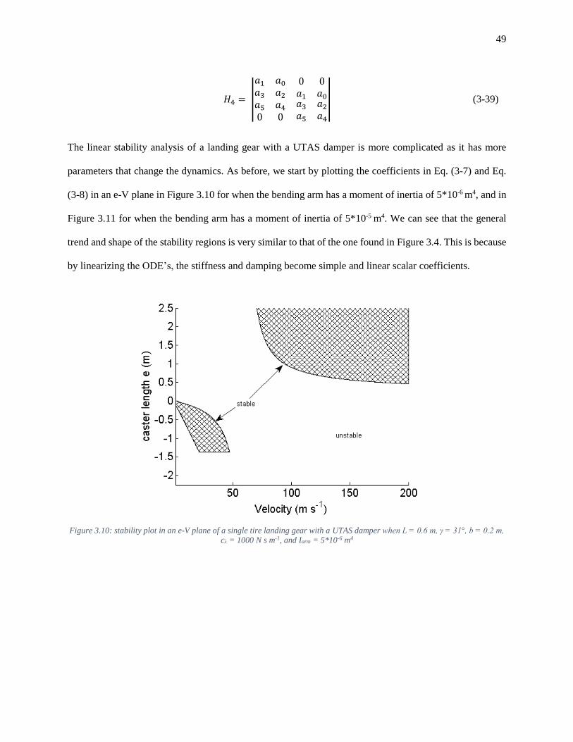
49

𝐻4 = |

𝑎1 𝑎0

𝑎3 𝑎2

0 0𝑎1 𝑎0

𝑎5 𝑎4

0 0

𝑎3 𝑎2

𝑎5 𝑎4

| (3-39)

The linear stability analysis of a landing gear with a UTAS damper is more complicated as it has more

parameters that change the dynamics. As before, we start by plotting the coefficients in Eq. (3-7) and Eq.

(3-8) in an e-V plane in Figure 3.10 for when the bending arm has a moment of inertia of 5*10-6 m4, and in

Figure 3.11 for when the bending arm has a moment of inertia of 5*10-5 m4. We can see that the general

trend and shape of the stability regions is very similar to that of the one found in Figure 3.4. This is because

by linearizing the ODE’s, the stiffness and damping become simple and linear scalar coefficients.

Figure 3.10: stability plot in an e-V plane of a single tire landing gear with a UTAS damper when L = 0.6 m, γ = 31°, b = 0.2 m,

cλ = 1000 N s m-1, and Iarm = 5*10-6 m4

50

Figure 3.11: stability plot in an e-V plane of a single tire landing gear with a UTAS damper when L = 0.6 m, γ = 31°, b = 0.2 m,

cλ = 1000 N s m-1, and Iarm = 5*10-5 m4

Changing velocity

Again, we switch to a 𝑐𝜆 − 𝑘𝜆 plane to have a better insight into the damper itself. For the UTAS damper,

the stiffness comes from the bending of the arm. So, the area moment of inertia of the arm is placed in the

x-axis instead of a stiffness coefficient. The inertia of the arm can give us an insight into the size of the

cross sectional area of the arm and its weight (knowing its length). In Figure 3.12, every parameter is kept

the same except for the velocity. Lower velocities tend to make the system unstable for lower stiffness

values (lower arm moment of inertia). However, as the velocity increases, there is little impact on

changing the stiffness (or moment of inertia of the arm), and stability is more dependent on the damping

alone.

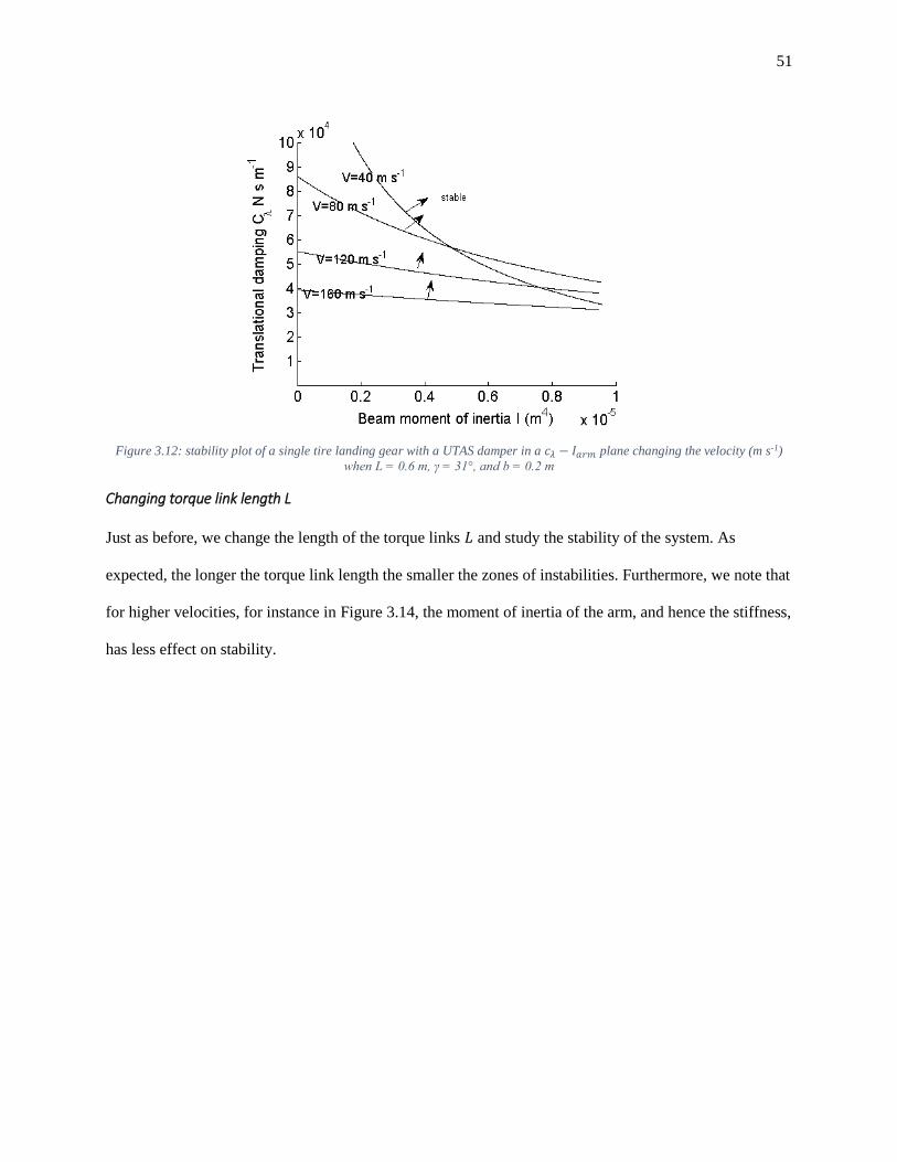
51

Figure 3.12: stability plot of a single tire landing gear with a UTAS damper in a 𝑐𝜆 − 𝐼𝑎𝑟𝑚 plane changing the velocity (m s-1)

when L = 0.6 m, γ = 31°, and b = 0.2 m


Just as before, we change the length of the torque links 𝐿 and study the stability of the system. As

expected, the longer the torque link length the smaller the zones of instabilities. Furthermore, we note that

for higher velocities, for instance in Figure 3.14, the moment of inertia of the arm, and hence the stiffness,

has less effect on stability.

52

Figure 3.13: stability plot of a single tire landing gear with a UTAS damper in a 𝑐𝜆 − 𝐼𝑎𝑟𝑚 plane changing the torque link length

L (m) and with V = 40 m s-1, b = 0.2 m, γ = 31°, and E = 200 GPa

Figure 3.14: stability plot of a single tire landing gear with a UTAS damper in a 𝑐𝜆 − 𝐼𝑎𝑟𝑚 plane changing the torque link length

L (m) and with V = 100 m s-1, b = 0.2 m, γ = 31°, and E = 200 GPa

Changing arms side distance b

A peculiar parameter of the UTAS damper is the distance at which the bending arm and damper are placed

away from the center of the assembly. This distance is denoted by 𝑏 in this thesis, see Figure 3.8. In Figure

3.15 and Figure 3.16 , the stability regions are obtained by changing this distance 𝑏 and keeping every other

53

parameter constant. As it is expected, the farther away from the center, and the bigger the 𝑏 parameter, the

smaller the stability region as the damper can apply less of its damping force; look at Eq. (3-29). This is

one of the drawbacks of this type of damper which has the damper element placed at an angle with respect

to the remaining torque link. This effect is less noticeable at lower velocities such as in Figure 3.15, but

more present at higher velocities such as in Figure 3.16.

Figure 3.15: stability plot of a single tire landing gear with a UTAS damper in a 𝑐𝜆 − 𝐼𝑎𝑟𝑚 plane changing the side length b (m)

when L = 0.6 m, γ = 31°, V = 40 m s-1, and E = 200 GPa

54

Figure 3.16: stability plot of a single tire landing gear with a UTAS damper in a 𝑐𝜆 − 𝐼𝑎𝑟𝑚 plane changing the side length b (m)

when L = 0.6 m, γ = 31°, V = 100 m s-1, and E = 200 GPa

Changing modulus of elasticity of arm E

The stiffness of the bending arm also depends on the type of material used. A comparison between

commonly used materials is crucial to see their performance, see Figure 3.17 and Figure 3.18.

Figure 3.17: stability plot of a single tire landing gear with a UTAS damper in a 𝑐𝜆 − 𝐼𝑎𝑟𝑚 plane changing young’s modulus of

the bending arm when L = 0.6 m, V = 40 m s-1, b = 0.2 m, and γ = 31°

Figure 3.18: stability plot of a single tire landing gear with a UTAS damper in a 𝑐𝜆 − 𝐼𝑎𝑟𝑚 plane changing young’s modulus of

the bending arm when L = 0.6 m, V = 100 m s-1, b = 0.2 m, and γ = 31°

55

It is obvious that carbon fiber is the best option as it performs almost like steel, but weights much less.

Weight is an important factor when designing shimmy dampers and should be taken into consideration

when doing so. Although it is outside the scope of this thesis, fatigue is also important to take into

consideration as this design would make the arm be under a dynamic load.

We also note that the curves converge at a single point when the moment of inertia of the arm is zero.

This is obvious because the elasticity of the arm influences the bending arm and not the damping element,

thus if there was no arm, meaning a moment of inertia of zero, the stability charts would only depend on

the damping coefficient.

3.5 New design

3.5.1 New shimmy damper design dynamics analysis

A new shimmy damper is proposed in this thesis and designed using the knowledge gathered from the

stability plots in this chapter, and also from the dynamic responses of the different shimmy dampers

obtained later in Chapter 4. The new design incorporates elements from the ones previously shown. For

example, one of the key issues with the Boeing damper is the freeplay between the torque links. This

phenomenon, studied by other researchers in [2] and [5], introduces further unwanted instabilities into the

system. The new and improved design takes this into account, and eliminates the possibility of having

freeplay by attaching both the spring and damping elements to the remaining torque link via a spherical

joint. The force from the damping element is maximized by placing it perpendicular to the remaining torque

link, something that was proven to be better in this chapter by comparing the dampers before. In addition,

a flexible beam is used as a spring, serving as the structural linkage and as the spring. The damper is placed

between the spherical joint and a stiff arm that extrudes to one side. The following figures will further show

how this new design works.

56

Figure 3.19: New shimmy damper design parts

When the tire starts shimmying and vibrating laterally, the lower part of the landing gear strut rotates,

making the remaining torque link to rotate as well. This action not only makes the arm bend, but it also

compresses or extends the damper. The actions of compression and extension of the damper are shown in

Figure 3.20.

Remaining torque

link

Bending arm

Damper

Rigid support

for damper

Spherical

joint

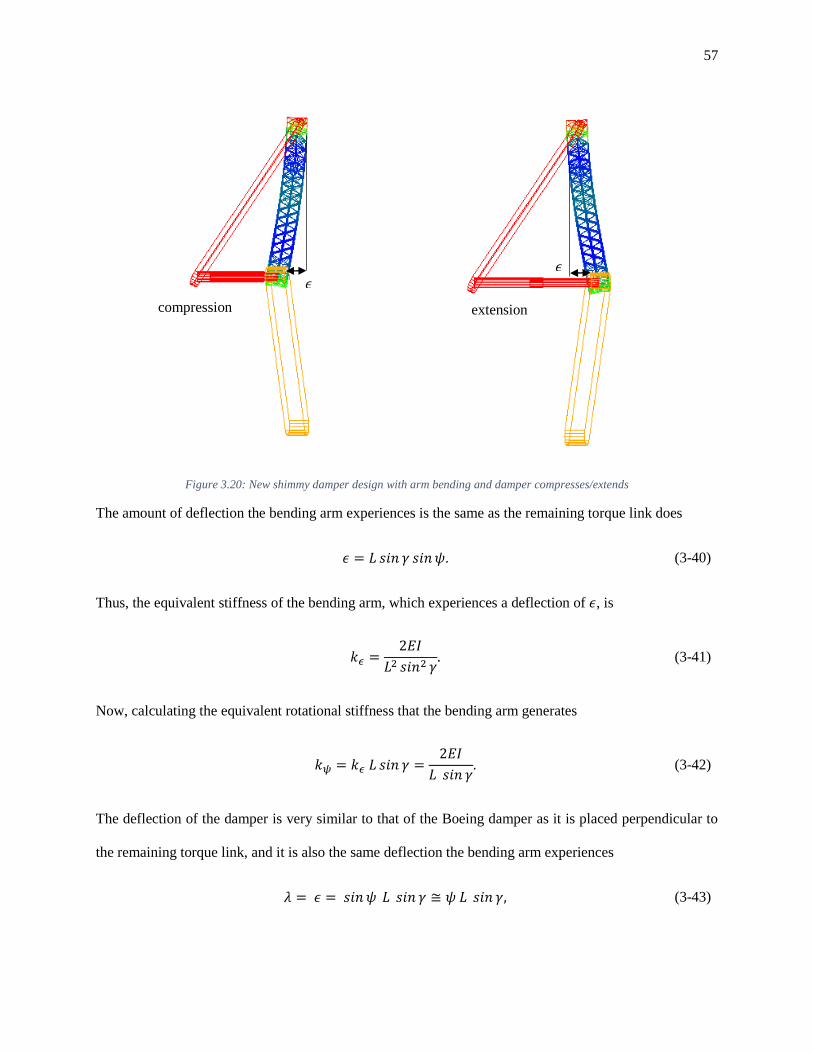
57

Figure 3.20: New shimmy damper design with arm bending and damper compresses/extends

The amount of deflection the bending arm experiences is the same as the remaining torque link does

𝜖 = 𝐿 𝑠𝑖𝑛 𝛾 𝑠𝑖𝑛𝜓. (3-40)

Thus, the equivalent stiffness of the bending arm, which experiences a deflection of 𝜖, is

𝑘𝜖 =

2𝐸𝐼

𝐿2 𝑠𝑖𝑛2 𝛾. (3-41)

Now, calculating the equivalent rotational stiffness that the bending arm generates

𝑘𝜓 = 𝑘𝜖 𝐿 𝑠𝑖𝑛 𝛾 =

2𝐸𝐼

𝐿 𝑠𝑖𝑛 𝛾. (3-42)

The deflection of the damper is very similar to that of the Boeing damper as it is placed perpendicular to

the remaining torque link, and it is also the same deflection the bending arm experiences

𝜆 = 𝜖 = 𝑠𝑖𝑛 𝜓 𝐿 𝑠𝑖𝑛 𝛾 ≅ 𝜓 𝐿 𝑠𝑖𝑛 𝛾, (3-43)

𝜖

𝜖

compression extension

58

�̇� = 𝑐𝑜𝑠 𝜓 �̇�𝐿 𝑠𝑖𝑛 𝛾 + 𝑠𝑖𝑛𝜓 𝐿 𝑐𝑜𝑠 𝛾 �̇� ≅ �̇�𝐿 𝑠𝑖𝑛 𝛾. (3-44)

Therefore, the equivalent rotational damping coefficient is

𝑐𝜓 = 𝑐𝜆𝐿2 𝑠𝑖𝑛2 𝛾. (3-45)

The linear ODE of a single tire landing gear with the new damper design proposed in this thesis is

𝐼𝑧�̈� +

2𝐸𝐼

𝐿 𝑠𝑖𝑛 𝛾𝜓 + 𝑐𝜆𝐿

2 𝑠𝑖𝑛2 𝛾 𝜓 ̇ + 𝐹𝑦𝑒 + 𝑀𝑧 + 𝑀𝜅 = 0. (3-46)

3.5.2 New shimmy damper design linear stability analysis

To perform a linear stability analysis, the Routh-Hurwitz determinants and the coefficients of the

characteristic equation of this system are calculated as follows

𝑎0 = 𝐼𝑥𝐼𝑧𝑉𝜎 (3-47)

𝑎1 = 𝐼𝑥𝐼𝑧𝑉2 − 𝐼𝑥𝜅𝜎 + 𝑐𝜆𝐿

2 𝑠𝑖𝑛2 𝛾 𝐼𝑥𝑉𝜎 + 𝑐𝑦𝐼𝑧𝑉𝜎 (3-48)

𝑎2 = (𝐼𝑥𝑉 + 𝑐𝑦𝜎)(𝑐𝜆𝐿

2 𝑠𝑖𝑛2 𝛾 𝑉 − 𝜅) + 𝑐𝑦𝐼𝑧𝑉2 + 𝐼𝑧𝑉(𝑐𝑦𝑉 + 𝑘𝑦𝜎) +

2𝐼𝑥𝐸𝐼𝑎𝑟𝑚𝑉𝜎

𝐿2 𝑠𝑖𝑛2 𝛾

+ 𝐶𝑓𝛼𝐹𝑧𝐼𝑧𝑉𝑙𝑔2 + 𝐹𝑧𝐼𝑥𝑉(𝐶𝑓𝛼𝑒 − 𝐶𝑚𝛼)(𝑒 − 𝑎)

(3-49)

𝑎3 = (𝑐𝑦𝑉 + 𝑘𝑦𝜎)(𝑐𝜆𝐿

2 𝑠𝑖𝑛2 𝛾 𝑉 − 𝜅) + 𝐼𝑧𝑘𝑦𝑉2 + 𝑙𝑔2𝐹𝑧(−𝐶𝑓𝛼𝜅 + 𝐶𝜆𝐿

2 𝑠𝑖𝑛2 𝛾 𝑉)

+2𝐸𝐼𝑎𝑟𝑚𝑉

𝐿2 𝑠𝑖𝑛2 𝛾(𝐼𝑥𝑉 + 𝑐𝑦𝜎) + 𝐹𝑧𝐼𝑥𝑉

2(𝐶𝑓𝛼𝑒 − 𝐶𝑚𝛼)

+ 𝑐𝑦𝐹𝑧𝑉(𝐶𝑓𝛼𝑒2 + 𝐶𝑚𝛼𝑎) − 𝑐𝑦𝐹𝑧𝑉(𝐶𝑚𝛼𝑒 + 𝐶𝑓𝛼𝑎𝑒)

(3-50)

𝑎4 = 𝑘𝑦𝑉(𝑐𝜆𝐿

2 𝑠𝑖𝑛2 𝛾 𝑉 − 𝜅) +2𝐸𝐼𝑎𝑟𝑚𝑉

𝐿2 𝑠𝑖𝑛2 𝛾(𝑐𝑦𝑉 + 𝑘𝑦𝜎 + 𝑙𝑔

2𝐶𝑓𝛼𝐹𝑧) + (𝐶𝑓𝛼𝑒

− 𝐶𝑚𝛼)(𝑐𝑦𝐹𝑧𝑉2 + 𝐹𝑧𝑘𝑦𝑉(𝑒 − 𝑎))

(3-51)

59

𝑎5 =

2𝐸𝐼𝑎𝑟𝑚𝑉2𝑘𝑦

𝐿2 𝑠𝑖𝑛2 𝛾+ 𝐹𝑧𝑉

2𝑘𝑦(𝐶𝑓𝛼𝑒 − 𝐶𝑚𝛼) (3-52)

H2 = |𝑎1 𝑎0

𝑎3 𝑎2| (3-53)

𝐻4 = |

𝑎1 𝑎0

𝑎3 𝑎2

0 0𝑎1 𝑎0

𝑎5 𝑎4

0 0

𝑎3 𝑎2

𝑎5 𝑎4

| (3-54)

We proceed once again to produce the stability charts of this shimmy damper design using the expressions

shown above. The first two figures shown now are obtained by plotting the expressions from before in an

e-V plane, where the moment of inertia of the bending arm used for the plot in Figure 3.21 is 10-5 m4, while

in Figure 3.22 it is 10-6 m4.

Figure 3.21: stability plot in an e-V plane for a single tire landing gear using the new and improved shimmy damper with

cλ=1000 N s m-1, and Iarm=1*10-6

60

Figure 3.22: stability plot in an e-V plane for a single tire landing gear using the new and improved shimmy damper with

cλ=1000 N s m-1, and Iarm=1*10-5

We can compare Figure 3.21 with Figure 3.10, and Figure 3.22 with Figure 3.11, and see how much the

new shimmy damper has increased the regions of stability. The bottom region of the graphs, where the

caster length is negative, has little importance and meaning to real world landing gears as negative casters

are seldom used when designing landing gears, and even less in main, non-steerable, landing gears. The

region of interest, the top part of the charts when the caster length is positive, shows that for low velocities

the system is unstable, just as shown before. However, with this improved design the area of stability is

much bigger than before. Note that this comparison is done for the same values of damping coefficient and

moment of inertia of the bending arm.

Changing velocity

Now, the charts of stability are plotted in a 𝑐𝜆 − 𝐼𝑎𝑟𝑚 plane, where 𝐼𝑎𝑟𝑚 represents the moment of inertia

of the bending arm. By keeping every single parameter constant except for the velocity of the system we

see its influence on this new design. Surprisingly enough, the new design yields stability regions that are

closer together to one another. In addition, it can be noted that the damping coefficient needed to obtain a

similar stability chart is significantly reduced.

61

Figure 3.23: stability plot of a single tire landing gear with the new shimmy damper in a 𝑐𝜆 − 𝐼𝑎𝑟𝑚 plane changing the velocity

(m s-1)


Now, the length of the torque link is changed to see its effect on the stability of the system with the new

shimmy damper. We can see from Figure 3.24 that, once again, the new and improved shimmy damper

design yields similar stability regions for different lengths of the torque link. It is obvious that having a very

short torque link is not a good idea, but it can be seen that for the other two lengths, when 𝐿 is 0.6 m and 1

m the stability regions are quite similar. In addition, at high moments of inertia of the arm, this difference

becomes even more negligible.

62

Figure 3.24: stability plot of a single tire landing gear with the new shimmy damper in a 𝑐𝜆 − 𝐼𝑎𝑟𝑚 plane changing torque link

length L (m) when V = 40 m s-1, E = 200 GPa

Figure 3.25: stability plot of a single tire landing gear with the new shimmy damper in a 𝑐𝜆 − 𝐼𝑎𝑟𝑚 plane changing torque link

length L (m) when V = 100 m s-1, E = 200 GPa

Changing modulus of elasticity of arm E

Now, the modulus of elasticity’s effect on systems stability is studied by changing its value and plotting the

different stability regions in a 𝑐𝜆 − 𝐼𝑎𝑟𝑚 plane for a velocity of 40 m s-1 in Figure 3.26, and 100 m s-1 in

Figure 3.27.

63

Figure 3.26: stability plot of a single tire landing gear with the new shimmy damper in a 𝑐𝜆 − 𝐼𝑎𝑟𝑚 plane changing the elasticity

of the bending arm E (GPa) when V = 40 m s-1

Figure 3.27: stability plot of a single tire landing gear with the new shimmy damper in a 𝑐𝜆 − 𝐼𝑎𝑟𝑚 plane changing the elasticity

of the bending arm E (GPa) when V = 100 m s-1

The difference in stability regions is even smaller when changing the elasticity of the arm. Also, we see the

lower damping coefficient needed, when compared to Figure 3.17. This new shimmy damper design is great

as it allows to use a lighter material, which is usually less stiff, and still have the same stability map as it

would when using a heavier, stiffer, arm.

Changing torque link angle γ

A stability chart is also developed to study the effect the angle γ has on stability. In Figure 3.29 below all

the curves meet for relatively big moment of inertia values, while for Figure 3.28 all the curves almost

64

meet for any value of damping coefficient or moment inertia. This tells us that the lower the velocity, the

less impact the torque link angle has on stability.

Figure 3.28: stability plot of a single tire landing gear with the new shimmy damper in a 𝑐𝜆 − 𝐼𝑎𝑟𝑚 plane changing γ when E =

200 GPa and V = 40 m s-1

Figure 3.29: stability plot of a single tire landing gear with the new shimmy damper in a 𝑐𝜆 − 𝐼𝑎𝑟𝑚 plane changing γ when E =

200 GPa and V = 100 m s-1

65

Chapter 4 Multibody model of landing gear

After studying the stability of a single tire landing gear with different shimmy dampers, the next step is to

look at the dynamic response of the system for stable and unstable behaviours. The numerical model

proposed in this thesis is built in a multibody dynamics software. MSC Adams is chosen as the

commercially available software to be used for this project. This software is vastly used in the automotive

and aerospace industry to study the dynamics and kinematics of moving objects with great detail. MSC

Adams also has a software package that deals specifically with tires called Adams/Tires. Many popular tire

models are integrated into the software and can be used along with the mechanical model of a landing gear,

as shown in Chapter 2. However, the model used in this thesis is the one of the stretched string, and not one

provided by Adams. The stretched string model will be input into Adams and will be used as the chosen

tire model for all the simulation investigations in this thesis. The stretched string model is the one used in

the simulation investigations because it can be validated using existing literature results.

4.1 Multibody model

The different parts that make the landing gear multibody model are: the mass of the aircraft, which could

be represented by a point mass or a constant force; the upper strut and the lower piston; the torque links;

the tire/s; the appropriate constraints/joints that hold these parts together; and the external and internal

forces that act on the system. Each of the rigid bodies is represented as a mass and inertia value obtained

from the literature. The geometry, weights, and other parameters are obtained from the literature as well

and are very close to real life landing gear values. The differential equations of motion of the moving bodies

can be found using the Lagrange equations seen below. However, MSC Adams does this systematically

and automatically. Using a general coordinate system, and local coordinate systems for each rigid body,

66

Adams is able to calculate all the required kinetic and potential energies of each body using the following

equations

𝑑

𝑑𝑡(

𝜕𝐿

𝜕�̇�𝑘) −

𝜕𝐿

𝜕𝑞𝑘= 𝑄𝑘 , (4-1)

where

𝐿 = 𝑇 − 𝑉, (4-2)

and 𝑇 is the kinetic energy of the system, 𝑉 the potential energy of the system, 𝑞𝑘 is the generalized

coordinate, 𝑄𝑘 is the generalized force, and 𝐿 the Lagrange function.

4.1.1 Joints and constraints

The landing gear multibody model has different types of constraints that are imposed to describe the

dynamics and kinematics of the moving parts with respect to each other. Each type of constraint has

equations related to them depending on their type. The most used constraints in the landing gear multibody

model developed in this thesis are presented below.

The revolute joint is the most used joint which removes five degrees of freedom, only letting a part I rotate

with respect to another part J about a single pivot axis. This joint is used on each tire, and in both sides of

the two torque links.

The cylindrical type of constraint is used for the main piston. The lower piston (part I) can translate inside

and out of the upper strut (part J), but it can also rotate with respect it. The cylindrical joint therefore

removes four degrees of freedom. If the vertical degree of freedom of the landing gear is omitted, then the

cylindrical joint is not used anymore. Instead, a simple revolute joint can replace it, eliminating the

translational vertical motion of the strut.

The inplane constraint removes one degree of freedom, the translational movement in a defined axis. The

model of the landing gear does not include the whole aircraft, therefore this constraint can be used to keep

the landing gear moving straight, without turning left or right.

67

The orientation constraint removes all three rotational degrees of freedom and is used to prevent the landing

gear upper strut from rotating. We assume the upper strut is cantilevered at the top, therefore this part cannot

rotate, as it models the rigid connection to the aircraft.

An easier way to constraint the model without using the previous two joints is to use a fixed constraint

where the top of the landing gear strut connects to the aircraft body. Here, we assume that the aircraft body

is moving with a constant velocity, thus it can be modelled as being stationary as no inertial forces will

affect the system.

4.1.2 Forces

When using the string tire model, tire forces have to be added manually to the tire body at the point where

it touches the ground. These forces are: the lateral force 𝐹𝑦, the self-aligning moment 𝑀𝑧, and the tire

damping moment 𝑀𝜅. All these forces and moments act on the same point on the tire body and are a

function of the slip angle, aircraft velocity, and rotation angle of the landing gear.

Apart from the forces developed by the tire, the landing gear itself has internal forces which can be taking

into account such as the landing gear shock strut. A linear spring-damper models the shock absorber of the

landing gear and transfers the force from the upper strut to the lower piston. This part of the landing gear is

crucial when landing and taking-off, as it dictates the normal force 𝐹𝑧 that acts on the tires. A translational

spring-damper element in Adams is used to model this device. When the vertical degree of freedom is

omitted in the model, no shock absorber force is used.

Furthermore, the shimmy dampers are also forces that can be modeled in Adams in two ways: as a rotational

damper-spring element, using only the rotational stiffness and damping coefficients, or using linear springs

and dampers with the proper shimmy damper geometry and linkages. The latter is the proper way of

modelling the shimmy dampers to study the effect of the different parameters of these dampers.

68

Other nonlinearities that are found in the system are, for instance, friction and mechanical freeplay. Adams

can accommodate for the nonlinearities we are interested in using different techniques. It is very important

to be able to incorporate these factors in the numerical model, as this will increase its accuracy significantly.

However, this thesis focuses in the linear analysis of landing gear systems, therefore these nonlinear

phenomena will be omitted.

4.2 Single tire landing gear model development for MSC Adams

Using the multibody dynamics software MSC Adams, we can create a model of a single tire landing gear

using the stretched string tire model, and then see the dynamic response and performance of the shimmy

dampers shown in Chapter 3 in stable and unstable conditions. The flexible beam in the UTC Aerospace

Systems damper is modeled using a Flex body from Adams. The rest of the parameters, unless otherwise

specified, are identical as the ones shown in Table 0.1.

The differential equation of the stretched string is input into Adams, as well as all the tire forces and

moments. The landing gear dynamics are handled automatically by the software. The dynamic response of

the system is obtained without linearization as Adams finds a numerical solution of the system’s ODEs. In

this thesis, the WSTIFF solver is used along with the Sl1 integrator in MSC Adams. The model is created

using rigid bodies connected together by joints. The bodies are shown in Figure 4.1, while the joints are

shown in Figure 4.2 and Figure 4.3.

69

Figure 4.1: Adams landing gear model: rigid bodies

Figure 4.2: Adams landing gear model joints

Aircraft body

Landing gear strut

Tire

Tire axle

Rotational strut

Fixed joint between tire

and axle

Fixed joint between strut

and axle

Revolute joint

torsional DOF ψ

70

Figure 4.3: Adams landing gear model joints

The two degree of freedom system is attached to the ground at the top of the landing gear with a fixed

constraint. This represents the body of the aircraft itself. The forces and moments developed by the tire are

input manually and are dependent on the tire slip angle, see Figure 4.4. The differential equation of the

stretched string Eq. (2-4) is also given to Adams and is solved numerically, giving the solution of the tire

slip to the forces and moments equations on each iteration step.

Figure 4.4: Adams landing gear model forces and moments

Fixed joint with

ground

Lateral damping and

stiffness moment Revolute joint:

lateral DOF δ

Strut torsional

damping and stiffness

moment

Tire damping moment M4

and self-aligning moment Mz Tire side force Fy

Tire normal force Fz

Gravity

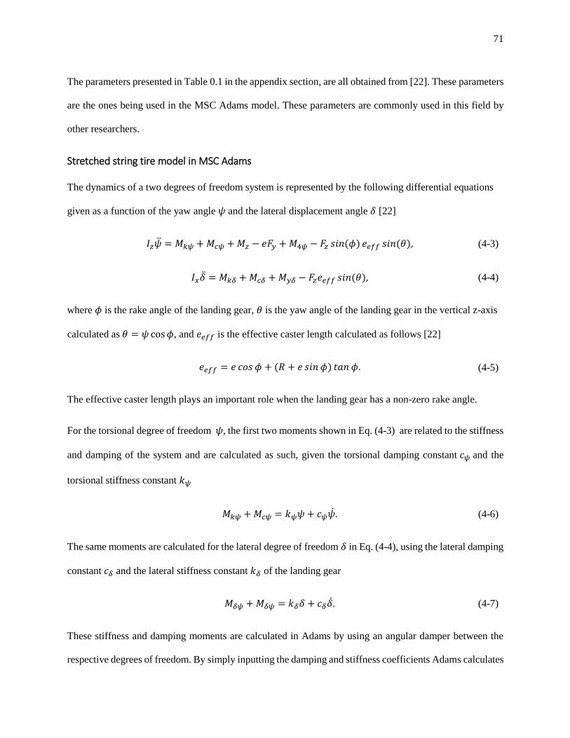
71

The parameters presented in Table 0.1 in the appendix section, are all obtained from [22]. These parameters

are the ones being used in the MSC Adams model. These parameters are commonly used in this field by

other researchers.

Stretched string tire model in MSC Adams

The dynamics of a two degrees of freedom system is represented by the following differential equations

given as a function of the yaw angle 𝜓 and the lateral displacement angle 𝛿 [22]

𝐼𝑧�̈� = 𝑀𝑘𝜓 + 𝑀𝑐𝜓 + 𝑀𝑧 − 𝑒𝐹𝑦 + 𝑀4𝜓 − 𝐹𝑧 𝑠𝑖𝑛(𝜙) 𝑒𝑒𝑓𝑓 𝑠𝑖𝑛(𝜃), (4-3)

𝐼𝑥�̈� = 𝑀𝑘𝛿 + 𝑀𝑐𝛿 + 𝑀𝑦𝛿 − 𝐹𝑧𝑒𝑒𝑓𝑓 𝑠𝑖𝑛(𝜃), (4-4)

where 𝜙 is the rake angle of the landing gear, 𝜃 is the yaw angle of the landing gear in the vertical z-axis

calculated as 𝜃 = 𝜓 cos𝜙, and 𝑒𝑒𝑓𝑓 is the effective caster length calculated as follows [22]

𝑒𝑒𝑓𝑓 = 𝑒 𝑐𝑜𝑠 𝜙 + (𝑅 + 𝑒 𝑠𝑖𝑛 𝜙) 𝑡𝑎𝑛 𝜙. (4-5)

The effective caster length plays an important role when the landing gear has a non-zero rake angle.

For the torsional degree of freedom 𝜓, the first two moments shown in Eq. (4-3) are related to the stiffness

and damping of the system and are calculated as such, given the torsional damping constant 𝑐𝜓 and the

torsional stiffness constant 𝑘𝜓

𝑀𝑘𝜓 + 𝑀𝑐𝜓 = 𝑘𝜓𝜓 + 𝑐𝜓�̇�. (4-6)

The same moments are calculated for the lateral degree of freedom 𝛿 in Eq. (4-4), using the lateral damping

constant 𝑐𝛿 and the lateral stiffness constant 𝑘𝛿 of the landing gear

𝑀𝛿𝜓 + 𝑀𝛿𝜓 = 𝑘𝛿𝛿 + 𝑐𝛿�̇�. (4-7)

These stiffness and damping moments are calculated in Adams by using an angular damper between the

respective degrees of freedom. By simply inputting the damping and stiffness coefficients Adams calculates

72

the respective displacements and compute the moments. When the shimmy dampers are being analysed,

the rotational spring 𝑘𝜓 and damper 𝑐𝜓 are changed to a linear spring 𝑘𝜆 and damper 𝑐𝜆 respectively.

The tire side force 𝐹𝑦 and the self-aligning moment 𝑀𝑧 are placed in Adams following the expressions given

in Eq. (2-10) and Eq. (2-12). These are nonlinear forces that are developed due to the tire’s elasticity.

Usually, they are normalized to simplify the modeling process. The self-aligning moment of the tire is input

into Adams as a piece-wise function [10]

𝑀𝑧 = {

𝐶𝑀𝛼 𝛼𝑚

𝜋𝑠𝑖𝑛(𝛼

𝜋

𝛼𝑚) 𝐹𝑧 , |𝛼| ≤ 𝛼𝑚

0, |𝛼| > 𝛼𝑚

, (4-8)

which depends on the self-aligning moment limit 𝛼𝑚 and the actual slip angle 𝛼. Furthermore, the side

force of the tire can be expressed using the slip angle 𝛼 and the tire’s normal force 𝐹𝑧 as it was shown before

in Eq. (2-10) [22]. Other ways of calculating the tire’s side force are shown in [10] and [6] yielding similar

results. Finally, the tire’s damping moment 𝑀𝜅 is expressed using Eq. (2-13) using the tire damping

coefficient denoted by κ [10].

Now, for the lateral degree of freedom, the only moment created due to the tire’s elasticity is a product of

the side force [22]

𝑀𝑦𝛿 = 𝑙𝑔𝐹𝑦 𝑐𝑜𝑠 𝜃 𝑐𝑜𝑠 𝜙. (4-9)

This moment is calculated by Adams automatically because it is part of the dynamics of the system. Finally,

the tire model is introduced in Adams by inputting the differential equation of the string Eq. (2-14).

Adams uses this equation and solves it, along with all the other equations of motion, obtaining a solution

for 𝑦1. The slip angle 𝛼 is then calculated using Eq. (2-9), which is then used to calculate all the other

quantities such as the side force 𝐹𝑦 and the self-aligning moment 𝑀𝑧.

73

4.3 Multibody model validation

Validation is an important part of any modelling work. Without it, one can never be sure of the accuracy of

the results obtained. Due to the nature of the work presented here, no experiments can be done to validate

the models. In this field, there is very little experimentation done as it is usually very expensive and difficult

to recreate, in a controlled environment, a landing gear with a tire landing or taking off at very high

velocities, reaching 300 km h-1, with very high loads.

The single tire landing gear multibody model developed in this thesis, which uses the stretched string theory

as a tire model, is validated using existing literature. More specifically, the results from Thota et al. [22]

are used to closely validate the results.

The graphs in the following sections show the simulation results from MSC Adams (left hand side), and

those from the reference Thota et al. [22] (right hand side). Both simulation results come from a single tire

landing gear model with only two degrees of freedom. Both models use the same landing gear and tire

parameters, which can be seen in Table 0.1 in the appendix section of this thesis. The only difference

between the models is that Adams handles the dynamics automatically, while in Thota et al. the dynamics

are explicitly described, having only two rotational degrees of freedom, and thus having two moments of

inertia. On the other hand, Adams, which takes care of the dynamics automatically, does not allow any

massless bodies, or those with only mass moments of inertia. Therefore, the simulation results from the

Adams model developed in this thesis and those from Thota et al. will not be exactly the same.

Velocity V = 40 m s-1, normal force Fz = 150 kN

The first simulation investigation is done with the parameters stated above. The top graphs in Figure 4.5

and Figure 4.6 show the angular rotation of the landing gear strut, while the bottom graphs show the

lateral translational displacement of the string and the lateral displacement of the landing gear itself. We

can see that the results from Adams in Figure 4.5 match perfectly with those from [22] shown in Figure

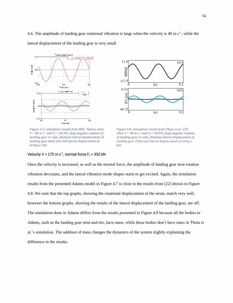
74

4.6. The amplitude of landing gear rotational vibration is large when the velocity is 40 m s-1, while the

lateral displacement of the landing gear is very small.


Once the velocity is increased, as well as the normal force, the amplitude of landing gear strut rotation

vibration decreases, and the lateral vibration mode shapes starts to get excited. Again, the simulation

results from the presented Adams model in Figure 4.7 is close to the results from [22] shown in Figure

4.8. We note that the top graphs, showing the rotational displacement of the struts, match very well,

however the bottom graphs, showing the results of the lateral displacement of the landing gear, are off.

The simulation done in Adams differs from the results presented in Figure 4.8 because all the bodies in

Adams, such as the landing gear strut and tire, have mass, while these bodies don’t have mass in Thota et

al.’s simulation. The addition of mass changes the dynamics of the system slightly explaining the

difference in the results.

Figure 4.5: simulation results from MSC Adams when

V= 40 m s-1 and Fz=150 kN, (top) angular rotation of

landing gear in rads, (bottom) lateral displacement of

landing gear delta*(m) and lateral displacement of

string y1 (m)

Figure 4.6: simulation results from Thota et al. [22]

when V= 40 m s-1 and Fz=150 kN, (top) angular rotation

of landing gear in rads, (bottom) lateral displacement of

landing gear δ*(m) and lateral displacement of string λ

(m)

75

Figure 4.7: simulation results from MSC Adams when V=

175 m s-1 and Fz= 350 kN, (top) angular rotation of landing

gear in rads, (bottom) lateral displacement of landing gear

delta*(m) and lateral displacement of string y1 (m)

Figure 4.8: simulation results from Thota et al. [22] when

V= 175 m s-1 and Fz= 350 kN, (top) angular rotation of


landing gear δ*(m) and lateral displacement of string λ (m)


Now, the velocity is decreased to see the interaction between the two modes of vibration: the yaw rotation

and the lateral bending of the strut. Once again, the yaw rotation of the strut results match almost

perfectly, while the results for the lateral bending of the strut have some discrepancies. Once again this is

explained with the difference in mass in the bodies. Another factor that changes the simulation results are

the initial conditions of the system. In the work by Thota et al. [22] none of the initial conditions are

mentioned, therefore some discrepancies might show between those results and the ones produced by the

model created in this thesis.

76

Figure 4.9: simulation results from MSC Adams when V=

155 m s-1 and Fz= 350 kN, (top) angular rotation of landing

gear in rads, (bottom) lateral displacement of landing gear

delta*(m) and lateral displacement of string y1 (m)

Figure 4.10: simulation results from Thota et al. [22] when

V= 155 m s-1 and Fz= 350 kN, (top) angular rotation of


landing gear δ*(m) and lateral displacement of string λ (m)

The last three simulation investigations show that the presented multibody model in this thesis can in fact

be used for shimmy analysis. Although the landing gear and tire parameters used were those from the

literature, these parameters have been used by other researchers as well in this area, and thus, we can use

them to explore shimmy with different types of shimmy dampers.

4.4 Simulation results

4.4.1 Boeing damper simulation

Just as it was done in the analytical portion of this thesis, the numerical model in Adams of this shimmy

damper does not include the freeplay or saturation nonlinearities. This way, we can make a better

comparison between the results from the analytical study in Chapter 3 and the numerical study in Chapter

4.

Looking at Figure 3.5, two points in the 𝑐𝜆 − 𝑘𝜆 plane are chosen to study the dynamic response of the

system. In the following figures, the angular displacement of the strut is shown as a function of time for

77

two different points in the 𝑐𝜆 − 𝑘𝜆 plane for different velocities respectively. The velocity is 40 m s-1 in

Figure 4.11, 80 m s-1 in Figure 4.12, and 160 m s-1 in Figure 4.13.

Figure 4.11: Adams simulation result using the Boeing damper for a velocity of 40 m s-1, L = 0.6 m, γ = 31°


78


We see that shimmy vibrations tend to decrease for higher velocities, just as suggested by the stability

plots. However, from Figure 3.5, we can see that the dynamic response doesn’t exactly correspond to the

stability charts. This happens for two main reasons. First, the landing gear multibody model used to get

the system’s dynamic response is more accurate and more complicated than the analytical model used to

get the stability charts. Also, these stability charts only show for certain the areas where the system are

unstable. Stability cannot be garanteed, which is why a dynamic response study is always needed.

4.4.2 UTAS damper simulation

A simulation investigation is also performed using the UTC Aerospace Systems damper model. Three

points in the 𝑐𝜆 − 𝐼𝑎𝑟𝑚 plane are chosen at a specific velocity, 40 and 80 m s-1, for two of the arm’s area

moment of inertia. We can see from Figure 4.14 that the damper successfully gets rid of the vibration for

a damping coefficient of 100,000 N s m-1, just as predicted by the stability chart in Figure 3.12. Any

lower value of the damping coefficient doesn’t mitigate the vibrations completely. Note that a much

larger damping coefficient is used for the UTAS damper, when compared to the Boeing damper, to

diminish the shimmy vibrations. This is one of the drawbacks of using this type of damper as it

ineffectively uses the damping force of the damping element by having it being placed at an angle to the

remaining torque link.

79

Figure 4.14: Adams simulation result using the UTAS damper for a velocity of 40 m s-1, b = 0.15 m, and Iarm = 3.4*10-6 m4


In Figure 4.16 the moment of inertia of the arm is changed to 8.3 * 10-6 m4, while every other parameter is

kept the same with respect to Figure 4.15. We see that at high velocities, the stiffness of the arm has a less

impact on the dynamic response and system stability.

80


We also note the asymmetry of vibration produced when using the UTAS shimmy damper. Due to the

asymmetry in parts, meaning having a bending arm to one side and a damping element on the other,

vibration tends to favor one side more than the other. Mainly, this has to do with the angle at which the

bending arm is placed, and how the remaining torque link pushes or pulls on this arm as the landing gear

strut rotates. Also note that when we increase the moment of inertia of the arm, the vibration asymmetry

decreases slightly because of the stiffer arm. This vibration asymmetry occurs because the bending arm

tends deflect more one side rather than the other due to the configuration of the remaining torque link and

its ability to rotate inwards, but almost impossible to rotate outwards.

4.4.3 New design damper simulation

The new shimmy damper design is modeled and simulated in MSC Adams to see its dynamic response

and the improvements on mitigating the shimmy vibrations. The following simulations are performed for

the velocities of 40, 80, and 160 m s-1, and when the moment of inertia of the arm is 3.4 *10-6 m4.

81

Figure 4.17: shimmy simulation using the new shimmy damper with different damping coefficients for when V = 40 m s-1, and

Iarm=3.4*10-6 m4


Iarm=3.4*10-6 m4

82


Iarm=3.4*10-6 m4

Although we can see that the frequency of vibration is larger when compared to the previous shimmy

dampers, the amplitude of vibration is generally much smaller. Also, there is no asymmetry in the

vibration as the damper itself and its parts are all symmetric. We can also note that the damping

coefficient needed to accomplish the same vibration mitigation action is much smaller when using the

new shimmy damper design. The following simulation is for a different arm’s moment of inertia.


Iarm=8.3*10-6 m4

83

When the moment of inertia is increased, such as in Figure 4.20, the vibration frequency tends to increase

from about 20 Hz in Figure 4.18, to about 30 Hz in Figure 4.3. However, the vibration amplitude

decreases significantly, and also does the amount of dampening coefficient needed to eliminate shimmy.

While 10 N s m-1 is enough to eliminate the vibrations when the moment of inertia of the arm is 8.3*10-6

m4 (Figure 4.20), it isn’t enough when the moment of inertia of the arm is 3.4*10-6 m4 (Figure 4.18).

84

Chapter 5 Discussions, conclusions, and future work

5.1 Discussion of results

The results of this thesis are divided in two parts: those for the stability charts, and those for the dynamic

response of the system. Each of these results show how some of the parameters of the system affect their

behaviour. We focus first on the stability charts developed in Chapter 3, and then on the dynamic

responses of each the dampers in Chapter 4.

The stability charts developed by the analytical expressions obtained for the tire and the landing gear are

of great importance as they give us a better understanding on the efficiency and performance of these

shimmy dampers. When comparing the e-V stability charts for the Boeing damper in Figure 3.4, for the

UTAS damper in Figure 3.10 and Figure 3.11, and for the new proposed damper in Figure 3.21 and

Figure 3.22, we can see that, overall, the latter has larger zones of stability. Now, when the stiffness and

damping values of the shimmy dampers are compared, as for example in Figure 3.5, Figure 3.12, and

Figure 3.23, the new proposed design again shows a more effective and robust design. The zones of

stability are closer together to each other when compared to the other two, and in general, the damping

coefficient needed is much lower. This means that the new proposed design won’t need a large heavy

damper, and the velocity of the aircraft won’t change the behaviour of the damper as much as it would for

the other two.

85

The dynamic responses of the each of the dampers is a useful way to see how these systems would behave

under different velocities. As it was mentioned before, the stability charts only say for sure when the

systems are unstable. Stability is never for certain, thus, picking different points in the stability charts for

these shimmy dampers lets us know if the system is in fact stable or not. We can compare the responses

for the Boeing damper in Figure 4.12, for the UTAS damper in Figure 4.15, and for the proposed damper

in Figure 4.18, all under the same velocity of 80 m s-1. The proposed shimmy damper needs a lower

damping coefficient to eliminate shimmy. Also, the UTAS damper shows asymmetrical vibrations.

However, we can note that the dynamic response for when using the proposed shimmy damper has a

higher frequency of vibration. This has to be taken into account when designing a shimmy damper for a

real life landing gear.

After having analyzed the two shimmy dampers presented in this thesis, one developed by Boeing and the

other by UTAS, using an analytical and a numerical approach, some recommendations are given for the

design of a new and improved damper. These recommendations are based on the results obtained by

performing the simulations and calculating the stability regions of the dampers by changing some of the

parameters. An insight into the effect these parameters have on stability is of great value as we can learn

how to design a better and improved shimmy damper. Two types of shimmy dampers were studied: one

that used a bending arm, and another that used a linear spring. The purpose of creating the stability regions

is to understand the effect different parameters like geometry, size, and stiffness or damping coefficient

would have on stability. The purpose of creating a multibody model is to understand and evaluate the

dynamic response of the system using different types of dampers while changing different parameters. With

all the information gathered, some recommendations are given for the design and development of a better

shimmy damper for main landing gears.

The first recommendation is related to the use of bending arms as spring elements. Through the different

simulations and results it was concluded that bending arms bring many advantages to shimmy dampers for

landing gears. A bending arm usually replaces an existing torque link and has two objectives: to serve as

86

the torque link it is replacing, and to act as a spring element. This way weight is not added to the system.

Having said that, the use of bending arms could also bring some problems. First, if any bending arms are

to be used in the design of a shimmy damper, such as the one used in the UTAS damper, it should be placed

as parallel as possible to the remaining torque link. This will prevent a shift in the vibration and will also

make sure that the bending mode of the arm is the only one being exited. In addition, less force will be used

to buckle the beam instead of bending it, increasing the performance, and decreasing its chance of failure.

As it was seen in Figure 4.14 and Figure 4.16, the vibration tends to shift to one side as there is an asymmetry

in the system. The remaining torque link, which pushes on the slanted bending arm, tends to rotate to one

side more than the other because the slanted bending arm bends more freely to this side. The shape of the

bending arm also plays a small role in the asymmetrical vibration of the damper. The remaining torque link

on the landing gear will always push the bending arm in one direction only, and that is perpendicular to the

torque link. The torque link’s ability to rotate inward also makes the bending arm vibrate more to one side,

making the torque link rotate even more to the inside. However, the torque link can’t rotate outwardly

because it is attach to an inextensible arm. Thus, placing the bending arm parallel to the remaining torque

link (meaning 𝑏 = 0 𝑚) would eliminate this problem, getting rid of the asymmetrical vibration.

The second recommendation is related to how the damping elements are attached to the landing gear and

to the remaining torque link. Dampers should be placed with a relatively large angle of attack, meaning

they should be prevented from being placed parallel to the remaining torque link. Instead, dampers should

be placed as perpendicular as possible to the remaining torque link, just as shown in the Boeing damper

design. This will maximize the use of the damping force acting on the remaining torque link, and it will

increase the amount of compression/extension on the damper. However, as we can see from Eq. (3-29), the

effective damping force changes as the torque link rotates. If the damping element is placed perpendicular

to the remaining torque link, the maximum effective damping force will be available right at the start of the

rotation of the torque link. On the other hand, if the damping element is placed slanted at some angle, just

at shown in the UTAS damper design, the maximum effective damping force will be available at some

87

other rotation angle of the strut 𝜓. We see that the effective damping force changes with the rotation angle

of the landing gear strut, therefore it is better if the damping element is placed perpendicular to the

remaining torque link.

The third recommendation has to do with creating a symmetrical shimmy damper. It seems more beneficial

to design a shimmy damper that is symmetrical about the landing gear strut rotation axis. For instance, the

Boeing damper is symmetrical as the spring and damper are in parallel to each other, and there is no

difference if the strut rotates clockwise or counter clockwise. On the other hand, the UTAS damper is

asymmetrical as a bending arm is placed on one side while a damping element is placed on the other side.

Just as it was shown in Figure 4.14 and Figure 4.16, asymmetrical vibrations are not desirable in landing

gear systems as they can induce uneven wear in joints and can fatigue parts in an irregular way.

The fourth and last recommendation is to try and eliminate any mechanical freeplay or any other nonlinear

phenomenon in the system. Just as shown in the Boeing damper, a mechanical freeplay exists to allow the

two torque links to move against each other, using the distance between them to place a spring and damper.

However, after this distance is travelled, no more damping force is developed. Thus, this type of damper

will only function for a small region of the rotational angle 𝜓. The proposed shimmy damper employs a

bending arm firmly connected through a spherical joint to the remaining torque link. This way, no

mechanical freeplay is present. Also, the damper is attached to the mentioned spherical joint in one side,

and to a fixed point in the other, eliminating any possibilities of saturation in the damping force.

The best shimmy damper design is the one that takes into account multiple factors such as: ease of

installation, manufacturability, and maintenance. These dampers should also be of low cost, low weight,

and high durability.

5.2 Conclusions

This thesis presents a linear stability analysis and the dynamic response of commonly used shimmy dampers

for main landing gears. The shimmy dampers from Boeing and UTC Aerospace Systems are used in this

88

work. Finally, a new and improved design of a shimmy damper is developed using the knowledge gathered

in this thesis.

The linear stability analysis is performed using the Routh-Hurwitz criterion. The stretched string tire model

is used along with the dynamics of a single tire landing gear and shimmy damper to fully describe the

system and obtain a mathematical expression that is used for stability analysis. The effect of different

parameters on system stability is the focus of this part of the thesis. Some of these parameters are: length

of torque link, velocity, stiffness and damping coefficient, elasticity of bending arm, and different

geometrical features. The landing gear’s velocity has a huge effect on system stability. However, it doesn’t

mean that the higher the velocity the more unstable the system. Depending on the system’s parameters,

shimmy occurs in a certain range of velocities, and stops happening when the velocity is relatively high.

Another factor that affects the stability regions is the torque link length, or any other parameter that changes

how far the shimmy damper acts from the rotation axis. The farther way the shimmy damper, the bigger the

torque it can produce. Thus, any parameter that makes this distance bigger will tend to increase the stability

of the landing gear. For shimmy dampers with bending arms, we learned that stiffness has an impact on

stability, but it can increase the weight of the device. Thus, depending on how much weight is allowed, the

choice of material is important because one with a high young’s modulus will tend to increase the stability

of the system, but could also add more weight.

A multibody model of a single tire landing gear is developed in Adams to show the dynamic response of

the different shimmy dampers used in the aerospace industry today. After validating the model using results

from the literature, the two shimmy damper designs are compared with the new and improved design shown

in this thesis. It is concluded that the proposed design is better in every possible aspect. The new shimmy

damper design needs a lower damping coefficient to mitigate the shimmy vibrations, in other words it

utilizes its resources more efficiently. Also, because of the amount of material needed it weighs the same,

or even less, than the competition. Furthermore, the new shimmy damper has a bending arm placed in the

same plane as the other torque link, and so no asymmetrical vibrations occur. Finally, the new design

89

doesn’t allow for freeplay between the torque links, which again is known to increase the chances for

shimmy.

One of the things noted during the stability analyses was that stiffness stops having an influence on stability

at higher velocity values. This can be used to our advantage to create active control systems on the damping

element which has more influence on system stability.

Overall, the new and improved shimmy damper design is better at creating larger zones of stability (Figure

3.21, Figure 3.22), at being more effective and needing a lower damping coefficient (Figure 3.23), and at

creating symmetrical vibrations that prevent things like uneven wear (Figure 4.18), while successfully

mitigating shimmy vibrations. This design has some trade-offs like the addition of weight due to the rigid

support arm needed to place the damping element, and the possibility of failure due to fatigue of the bending

arm.

5.3 Future work

To further increase the accuracy and fidelity of the models shown in this thesis, important aspects of the

system such as nonlinear effects could be incorporated. These nonlinear effects are usually omitted as they

are difficult to model, however, using a bifurcation analysis along with the software AUTO [44] makes it

possible for the study of these systems. Some examples of the nonlinearities that can be incorporated are

the freeplay and saturation found in the Boeing damper, and the nonlinear dynamics in the UTAS damper,

which can be studied using describing functions and bifurcation analysis.

The flexibility of the remaining torque link can be added to further increase the robustness of the analytical

model. For the model of the Boeing damper specifically, the flexibility of both torque links would be

needed. For the proposed damper, the flexibility of the rigid arm can be incorporated into the analytical

model.

90

A fatigue analysis would be beneficial for any shimmy damper that used a bending arm. These arms would

be in constant bending, and so a fatigue test would determine if the material, shape, and size of the bending

arm chosen would fail or not.

In addition, it would be important to add more tires into the analytical and numerical study of the landing

gear as this would further improve the accuracy and fidelity of the model. Depending on the amount of real

tires and their configuration, the use of the numerical approach with MSC Adams could be extremely

beneficial, in comparison with the highly complex analytical methods.

Finally, to further the research and the development of a perfect shimmy damper, an active control algorithm

could be implemented to control the damping coefficient of the damper element. It was noted through the

results of this thesis that at high velocities the stiffness of the shimmy damper stops having an effect on

stability. Therefore, a control system for the damper element would be beneficial. A common way to do

this would be to use a fluid damper filled with a magnetorheological fluid. The control algorithm would

control the viscosity of the fluid, and hence the damping coefficient, actively mitigating the shimmy

vibrations.

91

References

[1] P. D. Khapane, "Simulation of landing gear dynamics using flexible multi-body methods," in 25th

International Congress of the Aeronautical Sciences, 2006.

[2] C. Howcroft, M. Lowenberg and S. Neild, "Effects of Freeplay on Dynamic Stability of an Aircraft

Main Landing Gear," Journal of Aircraft, vol. 50, no. 6, pp. 1908-1922, 2013.

[3] W. Kruger, I. Besselink, D. Cowling, D. Doan, W. Kortum and W. Krabacher, "Aircraft Landing

Gear Dynamics: Simulation and Control," Vehicle System Dynamics, vol. 28, pp. 119-158, 1991.

[4] J. T. Gordon, "Perturbation Analysis of Nonlinear Wheel Shimmy," Journal of Aircraft, vol. 39, no.

2, pp. 305-317, 2002.

[5] C. Howcroft, M. Lowenberg, S. Neild, B. Krauskopf and E. & Coetzee, "Shimmy of an Aircraft

Main Landing Gear With Geometric Coupling and Mechanical Freeplay," Journal of

Computational and Nonlinear Dynamics, vol. 10, no. 5, p. 051011, 2015.

[6] H. Pacejka, Tyre and Vehicle Dynamics, Oxford: Butterworth-Heinemann, 2012.

[7] I. J. M. Besselink, "Shimmy of aircraft main landing gears," 2000.

[8] H. B. Pacejka, "The Wheel Shimmy Phenomenon," (Doctoral thesis), Delft University of

Technology, 1966.

[9] J. Wong, Theory of ground vehicles, John Wiley & Sons, 2001.

92

[10] G. Somieski, "Shimmy Analysis of a Simple Aircraft Nose Landing Gear Model Using Different

Mathematical Methods," Aerospace Science and Technology, vol. 8, pp. 545-555, 1997.

[11] G. Stepan, "Chaotic Motion of Wheels," Vehicle System Dynamics, vol. 20, pp. 341-351, 1991.

[12] G. Stepan, "Delay, nonlinear oscillations and shimmying wheels," Applications of Nonlinear and

Chaotic Dynamics in Mechanics, pp. 373-386, 1998.

[13] D. Takacs, G. Orosz and G. Stepan, "Delay effects in shimmy dynamics of wheels with stretched

string-like tyres," European Journal of Mechanics A/Solids, vol. 28, pp. 516-525, 2009.

[14] V. P. Zhuravlev, D. Klimov and P. K. Plotnikov, "A New Model of Shimmy," Mechanics of Solids,

vol. 48, no. 5, pp. 490-499, 2013.

[15] S. Ran, I. Besselink and H. Nijmeijer, "Application of nonlinear tyre models to analyse shimmy,"

Vehicle System Dynamics: International Journal of Vehicle Mechanics and Mobility, pp. 1-18,

2014.

[16] A. Fong, "Shimmy analysis of a landing gear system," Menasco Aerospace Ltd, Oakville, ON.

[17] P. D. Khapane, "SIMULATION OF AIRCRAFT LANDING GEAR DYNAMICS USING

FLEXIBLE MULTIBODY DYNAMICS METHODS IN SIMPACK," in Center, DLR-German

Aerospace.

[18] P. Khapane, "Simulation of Landing Gear Dynamics and Brake-Gear Interaction," in DLR-Interner

Bericht, 2008.

[19] K. Ogata, Modern Control Engineering, Prentice Hall, 2009.

93

[20] B. Goodwine and G. Stepan, "Controlling Unstable Rolling Phenomena," Journal of Vibration and

Control, vol. 6, pp. 137-158, 2000.

[21] P. Thota, B. Krauskopf and M. Lowenberg, "Multi-parameter bifurcation study of shimmy

oscillations in a dual-wheel aircraft nose landing gear," Nonlinear dynamics, vol. 70, pp. 1675-

1688, 2012.

[22] P. Thota, B. Krauskopf and M. Lowenberg, "Interaction of torsion and lateral bending in aircraft

nose landing gear shimmy," Nonlinear dynamics, vol. 57, pp. 455-467, 2009.

[23] T.-H. Huynh, G. Pouly, J.-P. Lauffenburger and M. Basset, "Active Shimmy Damping Using Direct

Adaptive Fuzzy Control," in Proceedings of the 17th World Congress The International Federation

of Automatic Control, Seoul, 2008.

[24] R. Van Der Valk and H. Pacejka, "An Analysis of a Civil Aircraft Main Gear Shimmy Failure,"

Vehicle System Dynamics, vol. 22, pp. 97-121, 1993.

[25] D. Takacs and G. Stepan, "Stability of towed wheels with elastic steering mechanism and shimmy

damper," Mechanical Engineering, vol. 51, no. 2, pp. 99-103, 2007.

[26] H. Chisholm, "Hydraulic steering motor and shimmy dampener for airplane landing gear wheels".

United States of America Patent 2,372,710, 3 April 1945.

[27] B. E. O'Connor, "Aircraft landing wheel shimmy damper". United States of America Patent

2,661,917, 8 December 1953.

[28] J. P. Labrecque, "Shimmy damper". United States of America Patent 3,430,896, 4 March 1969.

94

[29] R. D. Rumsey and R. E. King, "Shimmy damper for aircraft dual nosewheels". United States of

America Patent 3,424,406, 28 January 1969.

[30] R. D. Rumsey, "Linear type shimmy and steer damper". United States of America Patent 2,988,056,

13 June 1961.

[31] E. A. Kops and V. A. Johson, "Shimmy damper for airplane landing gear". United States of

America Patent 2,393,110, 15 January 1946.

[32] M. D. Etherton, "Shimmy damper for steerable aircraft wheel". United States of America Patent

2,714,429, 2 August 1955.

[33] W. S. Jensen, "Elastomer damper". United States of America Patent 6,290,038, 18 September 2001.

[34] P. J. Bachmeyer, D. A. Swanson, B. J. Pittman, S. K. Thompson and D. A. Hodgson, "Aircraft

landing gear assembly shimmy damper". United States of America Patent US 7,571,876 B2, 11

August 2009.

[35] W. E. Luce, "Shimmy damper for aircraft landing gear". United States of America Patent US

8,480,026 B2, 9 January 2013.

[36] D. W. Killian, "Active shimmy mitigation". United States of America Patent US 2012/0041660 A1,

16 February 2012.

[37] M. Besliu, "Hydraulic shimmy damper for aircraft landing gear". United States of America Patent

US 2013/0207327 A1, 15 August 2013.

[38] W. E. Boehringer, "Torque Linkage Damper". United States of America Patent 5,224,668, 6 July

1993.

95

[39] W. E. Luce, "Torque link with shimmy damper". United States of America Patent US 8,292,218 B2,

23 October 2012.

[40] N. S. Currey, Aircraft Landing Gear Design: Principles and Practices, Washington: American

Institute of Aeronautics and Astronautics, Inc., 1988.

[41] ADAMS/Tire help, ver2013.2.

[42] G. Gim, Vehicle dynamic simulation with a comprehensive model for pneumatic tires, PhD Thesis,

University of Arizona, 1988.

[43] R. Smiley and W. Horne, "Mechanical properties of pneumatic tires with special reference to

modern aircraft tires," NACA Report TR-R-64, 1960.

[44] E. Doedel, A. Champneys, T. Faigrieve, Y. Kusnetsov, B. Sandstede and X. Wang, "Auto 97:

continuation and bifurcation software for ordinary differential equations," May 2001. [Online].

Available: http://indy.cs.concodia.ca/auto/. [Accessed March 2015].

[45] P. Thota, B. Krauskopf and M. Lowenberg, "Influence of Tire Inflation Pressure on Nose Landing

Gear Shimmy," Journal of Aircraft, vol. 47, no. 5, pp. 1697-1706, 2010.

[46] H. Rahnejat, Multi-body Dynamics: Vehicles, Machines, and Mechanisms, Warrendale: Society of

Automotive Engineers, Inc., 1998.

96

Appendix

Table 0.1: Landing gear and tire parameters

Parameter Value Unit

Velocity V 0 – 200 m s-1

Half contact length a 0.1 m

Caster length e 0.12 m

Moment of inertia Iz 100 Kg m2

Lateral moment of inertia Ix 600 Kg m2

Vertical force Fz 150,000 N

Side force derivative Cfα 0.002 rad-1

Moment derivative CMα -1 m rad-1

Relaxation length σ = 3*a 0.3 m

Yaw stiffness kψ 380,000 N m rad-1

Yaw damping cψ 300 N m rad-1 s-1

Lateral stiffness ky 6,100,000 N m-1

Lateral damping cy 300 N s m-1

Length of landing gear lg 2.5 m

Rake angle φ 0 rad

Maximum slip angle αm 0.1745 rad

Damping coefficient of tire κ 570 N m2 rad -1

Arm’s young’s modulus E 200 MPa

Arm and damper side distance b 0.2 m

γ 0.541 (31°) rad

α 0.9948 (57°) rad

Bending arm length from the top R 0.368 m

Table 0.2: Fiala tire model input parameters [41]

Quantity Description Units Source

Vertical_damping Vertical damping coefficient N s

m

Tire property file (.tir)

Vertical_stiffness Vertical tire stiffness N

m


CSLIP Partial derivative of long. force (Fx) w.r.t. long.

slip ratio (S) at zero long. slip N Tire property file (.tir)

CALPHA Partial derivative of lateral force (Fy) w.r.t. slip

angle (α) at zero slip angle

N

rad


UMIN Coefficient of friction with full slip

(slip ratio = 1)

- Tire property file (.tir)

UMAX Coefficient of friction at zero slip - Tire property file (.tir)

Rolling_resistance Rolling resistance coefficient - Tire property file (.tir)

97

Table 0.3: UA tire model input parameters [41]

Quantity Units Description

Unloaded_radius r1 m Tire unloaded radius

Vertical_stiffness kz N

m

Vertical stiffness

Vertical_damping cz N s

m

Vertical damping

Rolling_resistance Cr m Rolling resistance parameter

CSLIP Cs N Longitudinal slip stiffness , ∂Fx

∂κ|κ=0

CALPHA Cα N

rad

Cornering stiffness, ∂Fy

∂α|α=0

CGAMMA Cγ N

rad

Camber stiffness, ∂Fy

∂γ|γ=0

Umin - Minimum friction coefficient

Umax - Maximum friction coefficient

REL_LEN_LON σx m Relaxation length in longitudinal direction

REL_LEN_LAT σy m Relaxation length in lateral direction

Table 0.4: Aircraft tire model inputs

Parameter Units Description

WIDTH W m Tire’s width

INFLATION_PRESSURE N

m2

Tire’s actual inflation pressure

RATED_PRESSURE N

m2

Tire’s rated inflation pressure

UNLOADED_RADIUS m Tire’s unloaded radius

VERTICAL_DAMPING N s

m

Vertical tire damping coefficient

ROLLING_RESISTANCE m Rolling resistance moment coefficient longitudinal

shift in the vertical centre of pressure during pure

rolling

UMAX - Coefficient of friction at zero slip

UMIN - Coefficient of friction when tire is sliding

V_UREF N

s

Reference velocity for friction coefficient

determination

RR_DELF_FACTOR - Factor used in the calculation of unbraked, unyawed

tire rolling radius

SLIP_STIFFNESS_FACTOR - Factor used in the calculation of slip stiffness, CSLIP

LON_DEFL_FACTOR - Reduction factor used in the calculation of longitudinal

shift in tire vertical centre of pressure

LAT_DEFL_FACTOR - Reduction factor used in the calculation of lateral shift

in tire vertical centre of pressure

FOOTPRINT_LENGTH_FACTOR - Reduction factor used in the calculation of the tire

footprint length

98

FOOTPRINT_AREA_RATIO - Ratio of net thread footprint area to gross tread

footprint contact area

linear stability analysis, dynamic response, and design of ... · shimmy dampers for main landing...

Documents