Production and Perception of Prosodic Events —Evidence from Corpus-based Experiments

Von der Philosophisch-Historischen Fakultat der Universitat Stuttgartzur Erlangung der Wurde eines Doktors der Philosophie (Dr. phil.)

genehmigte Abhandlung

Vorgelegt von

Antje Schweitzeraus Heidenheim-Schnaitheim

Hauptberichter: Prof. Dr. Bernd Mobius1. Mitberichter: Prof. Dr. Grzegorz Dogil2. Mitberichter: Prof. Dr. Elmar Noth

Tag der mundlichen Prufung: 10. Dezember 2010

Institut fur Maschinelle SprachverarbeitungUniversitat Stuttgart

2010

Erklarung

Hiermit erklare ich, dass ich, unter Verwendung der im Literaturverzeichnisaufgefuhrten Quellen und unter fachlicher Betreuung, diese Dissertationselbstandig verfasst habe.

(Antje Schweitzer)

Danksagung

Ich mochte mich an dieser Stelle bei den vielen Menschen bedanken, ohnederen Hilfe diese Arbeit niemals zustande gekommen ware.

Allen voran bei meinem Doktorvater Bernd Mobius; fur seine Geduld undsein Vertauen in mich; fur fruchtbare Diskussionen und Kommentare und dafur,dass er mir den notigen Freiraum gab; ganz besonders auch dafur, dass ichihn jederzeit mit Fragen uberfallen konnte, die auch noch prompt beantwortetwurden.

Bei Prof. Grzegorz Dogil, der mir immer den Rucken starkte und mir in denOhren lag, meine Ergebnisse zu veroffentlichen. Bei Elmar Noth, der sich sehrkurzfristig als Gutachter zur Verfugung stellte (auch wenn ihm dafur nur einBier in Aussicht gestellt wurde).

Bei Michael Walsh, der diese Arbeit Korrektur gelesen hat und dabei mitvielen wertvollen inhaltlichen Kommentaren beigetragen hat (und dafur nochnicht mal ein Bier haben wollte). Bei Sabine Schulte im Walde, die mirTipps und Skripts zur Auswertung meiner Ergebnisse gab, obwohl sie selbstgenug um die Ohren hatte. Bei Bernd Schwald, der mir half, eine vernunftigemathematische Notation fur die Evaluierungsmethode zu finden. Bei meinerBurogenossin Katrin Schneider fur ihre immerwahrende Hilfsbereitschaft, unddass sie es mit Gelassenheit ertrug, wenn ich beim Arbeiten mit mir selbst odermit meinem Computer redete. Außerdem bei allen anderen Kollegen der Ex-perimentellen Phonetik, nicht zuletzt fur die freundschaftliche Atmosphare.

Besonderer Dank gilt naturlich meiner Familie; insbesondere meinem Mann,der es mir nicht ubel nahm, dass ich die Abende mit dieser Arbeit statt mit ihmverbrachte.

Teile bzw. Aspekte dieser Arbeit wurden durch das BMBF im Rahmen derProjekte SmartKom und SmartWeb sowie durch die DFG im Rahmen des Pro-jekts “Prosodieproduktion” gefordert; ohne diese Projekte ware diese Arbeit sonicht moglich gewesen.

3

Contents

Abstract 10

Deutsche Zusammenfassung 13

1 Introduction 17

2 Perception and production in the segmental domain 212.1 Keating’s window model of coarticulation . . . . . . . . . . . . . 212.2 Guenther and Perkell’s model . . . . . . . . . . . . . . . . . . . . 232.3 Exemplar theory . . . . . . . . . . . . . . . . . . . . . . . . . . . 26

2.3.1 Storing exemplars in memory . . . . . . . . . . . . . . . . 262.3.2 Phonetic categories in exemplar theory . . . . . . . . . . 282.3.3 Exemplar-theoretic categorization . . . . . . . . . . . . . 292.3.4 Production in exemplar theory . . . . . . . . . . . . . . . 322.3.5 An exemplar version of Guenther and Perkell’s model . . . 362.3.6 Prosody in exemplar models . . . . . . . . . . . . . . . . . 37

3 Modeling intonation 393.1 GToBI(S) . . . . . . . . . . . . . . . . . . . . . . . . . . . . . . . 393.2 PaIntE . . . . . . . . . . . . . . . . . . . . . . . . . . . . . . . . . 43

3.2.1 Prosodic context . . . . . . . . . . . . . . . . . . . . . . . 453.2.2 F0 smoothing . . . . . . . . . . . . . . . . . . . . . . . . . 463.2.3 Approximation methods . . . . . . . . . . . . . . . . . . . 463.2.4 Check for plausibility . . . . . . . . . . . . . . . . . . . . . 483.2.5 Future improvements . . . . . . . . . . . . . . . . . . . . 49

4 The temporal targets in prosody production 514.1 Description of the speech data . . . . . . . . . . . . . . . . . . . . 524.2 A measure of local speech rate . . . . . . . . . . . . . . . . . . . . 554.3 Target regions for temporal z-scores . . . . . . . . . . . . . . . . 604.4 Temporal target regions and the syllabary . . . . . . . . . . . . . 68

4.4.1 Frequent and infrequent syllables . . . . . . . . . . . . . . 694.4.2 Dual-route phonetic encoding . . . . . . . . . . . . . . . . 70

4

Contents

4.4.3 The dual-route hypothesis in the temporal domain . . . . 714.5 Conclusion . . . . . . . . . . . . . . . . . . . . . . . . . . . . . . 74

5 The tonal dimension of perceptual space 765.1 Interpretation of the PaIntE parameters . . . . . . . . . . . . . . . 76

5.1.1 Peak alignment . . . . . . . . . . . . . . . . . . . . . . . . 805.1.2 Peak height . . . . . . . . . . . . . . . . . . . . . . . . . . 885.1.3 Amplitudes of rise and fall . . . . . . . . . . . . . . . . . . 93

5.2 Target regions for intonation events . . . . . . . . . . . . . . . . . 102

6 Modeling categorization 1056.1 Representing the data . . . . . . . . . . . . . . . . . . . . . . . . 106

6.1.1 Attributes . . . . . . . . . . . . . . . . . . . . . . . . . . . 1066.1.2 Databases for training and testing . . . . . . . . . . . . . . 1156.1.3 Noisy data . . . . . . . . . . . . . . . . . . . . . . . . . . . 117

6.2 Detecting prosodic categories . . . . . . . . . . . . . . . . . . . . 1186.2.1 Preliminary remarks . . . . . . . . . . . . . . . . . . . . . 1196.2.2 A first experiment . . . . . . . . . . . . . . . . . . . . . . 1246.2.3 Varying numbers of clusters . . . . . . . . . . . . . . . . . 1286.2.4 Evaluation of clustering results . . . . . . . . . . . . . . . 1326.2.5 Cross-validating the results . . . . . . . . . . . . . . . . . 1396.2.6 Discussion and Outlook . . . . . . . . . . . . . . . . . . . 151

6.3 Prediction of prosodic events . . . . . . . . . . . . . . . . . . . . 1556.3.1 Procedure . . . . . . . . . . . . . . . . . . . . . . . . . . . 1566.3.2 Syllable-based vs. word-based evaluation . . . . . . . . . 1576.3.3 Results . . . . . . . . . . . . . . . . . . . . . . . . . . . . . 1586.3.4 Generalizability . . . . . . . . . . . . . . . . . . . . . . . . 1646.3.5 Comparison with other studies . . . . . . . . . . . . . . . 1656.3.6 Comparison with human prosodic labeling . . . . . . . . . 1656.3.7 Illustrating the results . . . . . . . . . . . . . . . . . . . . 1666.3.8 Discussion and Outlook . . . . . . . . . . . . . . . . . . . 176

7 Conclusion and Outlook 178

5

List of Abbreviations

ERB Equivalent Rectangular Bandwidth

F0 Fundamental Frequency

F1 First Formant

F2 Second Formant

GToBI German Tones and Break Indices

GToBI(S) German Tones and Break Indices (Stuttgart version)

IMS Institute of Natural Language Processing

IPA International Phonetic Alphabet

LNRE Large Number of Rare Events

MLM Multilevel Exemplar Model

PaIntE Parametrized Intonation Events

POS Part-of-Speech Tag

STTS Stuttgart-Tubingen Tagset

ToBI Tones and Break Indices

TTS Text-to-speech Synthesis

VOT Voice Onset Time

6

List of Figures

2.1 Illustration of articulation windows . . . . . . . . . . . . . . . . . 222.2 Target region for American English /r/ . . . . . . . . . . . . . . . 252.3 F2 distributions of stored /E/ and /I/ instances . . . . . . . . . . 30

3.1 Schematic diagrams of the GToBI(S) pitch accents . . . . . . . . . 413.2 Schematic diagrams of the GToBI(S) boundary tones . . . . . . . 433.3 PaIntE approximation function . . . . . . . . . . . . . . . . . . . 443.4 Reducing the approximation window . . . . . . . . . . . . . . . . 47

4.1 Histogram of phoneme/context vectors . . . . . . . . . . . . . . . 544.2 Histograms of boundary tones and pitch accents . . . . . . . . . . 554.3 Histograms of durations . . . . . . . . . . . . . . . . . . . . . . . 574.4 “Elasticity” of different phoneme classes . . . . . . . . . . . . . . 584.5 Z-scores of accented nuclei and phrase-final segments . . . . . . . 614.6 Z-scores of phrase-final segments . . . . . . . . . . . . . . . . . . 624.7 Z-scores of segments in different syllable positions: boundaries . 634.8 Z-scores of segments in different syllable positions: accents . . . 644.9 Z-scores of accented and phrase-final syllables . . . . . . . . . . . 664.10 Z-scores of phrase-final syllables . . . . . . . . . . . . . . . . . . . 674.11 Mean z-scores in frequent vs. infrequent syllables . . . . . . . . . 73

5.1 PaIntE approximation function (repeated) . . . . . . . . . . . . . 775.2 Schematic diagrams of the GToBI(S) pitch accents (repeated) . . 785.3 Histograms of pitch accents and boundary tones . . . . . . . . . . 795.4 Distribution of the b parameter for accents . . . . . . . . . . . . . 815.5 Distributions of the b parameter for word-final vs. word-internal

L*H accents . . . . . . . . . . . . . . . . . . . . . . . . . . . . . . 835.6 Distributions of the b parameter for H*L in low, mid, and high

vowels . . . . . . . . . . . . . . . . . . . . . . . . . . . . . . . . 845.7 Distributions of the b parameter for boundaries . . . . . . . . . . 865.8 Distributions of the d parameter for accents . . . . . . . . . . . . 895.9 Disributions of the d parameter for L*H accents in different po-

sitions in the phrase . . . . . . . . . . . . . . . . . . . . . . . . . 91

7

List of Figures

5.10 Distributions of the d parameter for boundaries . . . . . . . . . . 925.11 Distributions of the c1 and c2 parameters for accents . . . . . . . 955.12 Distributions of the c1 parameter for unaccented syllables in the

neighborhood of pitch accents . . . . . . . . . . . . . . . . . . . . 965.13 Distributions of the b parameter for accents with c1>20 after L*H 975.14 Distributions of the b parameter for accents after unaccented syl-

lables with c1>20 . . . . . . . . . . . . . . . . . . . . . . . . . . . 985.15 Distributions of the c1 parameter for boundaries . . . . . . . . . . 1005.16 Distributions of the c2 parameter for boundaries . . . . . . . . . . 101

6.1 Classification accuracy rates for pitch accent clustering . . . . . . 1256.2 Classification accuracy rates on independent test data . . . . . . . 1276.3 Classification accuracy rates for 300 clusters experiment . . . . . 1316.4 v-measure results for pitch accent clustering . . . . . . . . . . . . 1346.5 v-measure results for 300 clusters experiment . . . . . . . . . . . 1366.6 v-measure results for 3200 clusters experiment . . . . . . . . . . 1386.7 v-measure results for 3000X experiment . . . . . . . . . . . . . . 1406.8 v-measure results for 10:90 experiment . . . . . . . . . . . . . . . 1436.9 v-measure results for 10:10 experiment . . . . . . . . . . . . . . . 1446.10 Classification accuracies for 10:10 experiment . . . . . . . . . . . 1466.11 Classification accuracies for 10:10 experiment, on independent

test data . . . . . . . . . . . . . . . . . . . . . . . . . . . . . . . 1476.12 Classification accuracies for 10:90 experiment, on independent

test data . . . . . . . . . . . . . . . . . . . . . . . . . . . . . . . 1486.13 Classification accuracies for 90:10 experiment . . . . . . . . . . 1496.14 Classification accuracies for 90:10 experiment, on independent

test data . . . . . . . . . . . . . . . . . . . . . . . . . . . . . . . 1506.15 Word-based accuracy rates for various machine learning schemes 1596.16 Screenshot: prediction results for utterance f001 . . . . . . . . . 1696.17 Screenshot: prediction results for utterance f011 . . . . . . . . . 1716.18 Screenshot: prediction results for utterance f021 . . . . . . . . . 1736.19 Screenshot: prediction results for utterance f041 . . . . . . . . . 175

8

List of Tables

5.1 Significance levels for comparing accent and boundary distribu-tions of the b parameter . . . . . . . . . . . . . . . . . . . . . . . 88

5.2 Significance levels for comparing accent and boundary distribu-tions for the d parameter . . . . . . . . . . . . . . . . . . . . . . 93

5.3 Significance levels for comparing accent and boundary distribu-tions for the c1 parameter . . . . . . . . . . . . . . . . . . . . . . 102

5.4 Significance levels for comparing accent and boundary distribu-tions for the c2 parameter . . . . . . . . . . . . . . . . . . . . . . 103

6.1 Example: attributes and observed values, part 1 . . . . . . . . . . 1076.2 Example: attributes and observed values, part 2 . . . . . . . . . . 1096.3 Example: attributes and observed values, part 3 . . . . . . . . . . 1106.4 Example: attributes and observed values, part 4 . . . . . . . . . . 1126.5 Example: attributes and observed values, part 5 . . . . . . . . . . 1136.6 Example: contingency table for 15 clusters, absolute frequencies . 1226.7 Example: contingency table for 15 clusters, relative frequencies . 1236.8 Word-based accuracy rates for the best algorithms . . . . . . . . . 1616.9 Word-based accuracy rates for instanced-based learning . . . . . 1636.10 Example: word-based prediction results for utterance f001 . . . . 1686.11 Example: word-based prediction results for utterance f011 . . . . 1706.12 Example: word-based prediction results for utterance f021 . . . . 1726.13 Example: word-based prediction results for utterance f031 . . . . 1746.14 Example: word-based prediction results for utterance f041 . . . . 174

9

Abstract

This thesis explores perception and production of prosody by way of corpus ex-periments. Following Dogil and Mobius (2001) I suggest to apply Guenther andPerkell’s speech production model for the segmental domain (Guenther 1995;Guenther et al. 1998; Perkell et al. 2001) to the prosodic domain. Guentherand Perkell argue that the targets in speech production take the form of multi-dimensional regions in auditory space (Guenther 1995; Guenther et al. 1998)or auditory-temporal space (Perkell et al. 2000). Speakers establish these tar-get regions in speech acquisition, as well as internal models for mapping fromarticulator reference frame to a perceptual planning reference frame. I suggestthat Guenther and Perkell’s model is compatible with exemplar theory, and thatthe target regions can be derived in an exemplar-theoretic fashion.

The key idea in exemplar theory as applied to speech (e.g. Lacerda 1995;Goldinger 1996, 1997, 1998; Johnson 1997; Pierrehumbert 2001, 2003) is thatspeakers have access to memory traces (“exemplars”) of previously perceivedinstances of speech in which almost full phonetic detail is retained. Linguisticknowledge on various linguistic levels then arises from abstracting over thestored exemplars (Pierrehumbert 2001, 2003). I suggest that target regionsin the sense of Guenther and Perkell are established in the same way: Theyare implicitly derived from the range of values that is observed for the storedexemplars in the relevant dimensions.

Applying Guenther and Perkell’s model to the prosodic domain, I assumethat the prosodic categories are the categories posited by GToBI(S) (Mayer1995) in adaptation of the Tone Sequence Model (Pierrehumbert 1980) toGerman. As for the dimensions of the target regions pertaining to these cat-egories, I suggest a measure of local speech rate, viz. duration z-scores, as thetemporal dimension, and tonal parameters describing the shape of F0 contoursrelated to prosodic categories, the so-called PaIntE parameters, as tonal dimen-sions. The duration z-scores are obtained by standardizing phone durationsusing phoneme-specific means and standard deviations. The tonal PaIntE pa-rameters are derived by approximating the F0 contour in a three-syllable win-dow around the syllable of interest using the PaIntE model (Mohler and Conkie1998). According to Guenther and Perkell, the relevant dimensions are percep-tual dimensions. To motivate the perceptual relevance of duration z-scores and

10

List of Tables

PaIntE parameters, realizations of prosodic categories in a large database areinvestigated by examining their distributions for each parameter. It is shownthat the parameters capture well-known aspects of the realization of prosodicevents, such as phrase-final lengthening related to prosodic phrases, the dif-ferences in the alignment of peaks and those between rise and fall amplitudesfor the different categories as predicted by GToBI(S), the optimal alignmentof peaks with syllable structure (House 1996), but also more recent findingssuch as the influence of vowel height on the alignment of peaks in GermanH*L accents (Jilka and Mobius 2007). Confidence tests confirm that for theprosodic categories, the parameter distributions observed in the corpus differsignificantly. This is taken as evidence that the parameters play a role in per-ception.

To further motivate this claim, I show that the parameters are useful in de-tecting prosodic categories automatically. Exemplar theory would suggest thatif all relevant perceptual dimensions are known, it should be straightforward todetect clouds corresponding to phonetic categories using clustering techniques.In this vein, Pierrehumbert (2003) reviews clustering results obtained by Kor-nai (1998) where clusters of F1/F2 data corresponded well to vowel categories.She posits that stable categories are characterized by “well-defined clusters orpeaks in phonetic space” (Pierrehumbert 2003, p. 210). To detect clusters cor-responding to prosodic categories, I conducted clustering experiments using aprosodically annotated corpus of a male speaker. For each syllable in the cor-pus, 29 attributes involving duration z-scores and PaIntE parameters as well asderived parameters and some additional higher-linguistic attributes were ex-tracted. The resulting data were clustered using various clustering algorithmsand various numbers of clusters.

To begin with, the experimental results show that it is in general possibleto identify clusters which correspond well to prosodic categories. Furthermore,if the clusters correspond to categories, they should generalize to new data.For evaluating the generalizability of the clusterings I suggest a new proce-dure which evaluates clusterings on independent test data using a classificationaccuracy measure which models exemplar-theoretic categorization: Accordingto exemplar theory, categorizing new instances in speech perception is basedon the stored exemplars and their categories (Lacerda 1995; Johnson 1997;Pierrehumbert 2001, 2003), i.e., categorization should be possible based onthe detected clusters and their categories. Two clustering algorithms, namelySimpleKMeans and FarthestFirst, perform similarly well with respect to thismeasure, reaching classification accuracies of slightly more than 85% on inde-pendent test data. This is clearly above the baseline of around 78%.

As for the number of clusters, these scores are reached for approximately1600 clusters in case of SimpleKMeans, and for approximately 2000 clusters incase of FarthestFirst, suggesting that these are appropriate numbers of clusters.Such high numbers of clusters may be unexpected at first. However, a one-

11

List of Tables

to-one correspondence of clusters to phonetic categories cannot be expected(Pierrehumbert 2003, p. 211). Also, there were altogether 29 attributes usedfor clustering. Thus, the clusters are detected in a 29-dimensional space. Rela-tive to the dimensionality of the clustering space, 1600 to 2000 clusters seemsmore appropriate than on first glance.

Finally, prosodic categorization is simulated using supervised machine learn-ing methods to classify new exemplars based on the same parameters as in theclustering experiments, again to corroborate their perceptual relevance. Sev-eral classification algorithms yield results of approx. 78% accuracy on the wordlevel for pitch accents, and approx. 88% accuracy on the word level for phraseboundaries, which compare very well to results reported in other recent stud-ies, particularly to results on German. The word level accuracies for pitch ac-cents correspond to approximately 87.5% on the syllable level, which is slightlybut not dramatically better than the accuracies of around 85% obtained abovefor the clusterings. The classifiers generalize well to similar data of a femalespeaker in that they perform equally well as classifiers trained directly on thefemale data. In contrast to most other studies, the classifiers predict the fullset of GToBI(S) labels rather than just two classes. These classifiers have beenintegrated into a prototype of a tool for automatic prosodic labeling. Some ex-amples of automatic prosodic annotations produced by this tool are given toillustrate its usefulness in automatic prosodic labeling.

In summary, the main contributions of this thesis are, (i), the applicationof an exemplar-theoretic interpretation of Guenther and Perkell’s speech pro-duction model to the prosodic domain, (ii), a set of perceptually relevant pa-rameters which capture tonal and temporal aspects of the implementation ofprosodic events, (iii), an extensive investigation of the GToBI(S) prosodic cat-egories in terms of these parameters, (iv), a measure to evaluate the general-izability of cluster results to new data, (v), a prototype of a tool for automaticprosodic labeling.

12

Deutsche Zusammenfassung

Diese Arbeit beschaftigt sich mit Korpusexperimenten zur Perzeption und Pro-duktion von Prosodie. Ich folge Dogil und Mobius (2001) und schlage vor,Guenther and Perkells Sprachproduktionsmodell fur die segmentale Ebene(Guenther 1995; Guenther et al. 1998; Perkell et al. 2001) auf die Ebene derProsodie zu ubertragen. Guenther und Perkell vertreten die Meinung, dass Pro-duktionsziele in der Sprachproduktion durch multidimensionale Zielregionenim auditorischen (Guenther 1995; Guenther et al. 1998) oder auditorisch-temporalen Raum (Perkell et al. 2000) reprasentiert werden. Sprecher erler-nen diese Zielregionen beim Spracherwerb, ebenso wie interne Modelle, die esdem Sprecher erlauben, Produktionsgesten von einem artikulatorischen Refe-renzrahmen auf einen perzeptuellen Referenzrahmen abzubilden. Ich schlagevor, dass Guenther und Perkells Modell mit der Exemplartheorie kompatibelist, und dass die Zielregionen mithilfe exemplartheoretischer Prozesse erlerntwerden konnen.

Die zentrale Idee bei der Anwendung der Exemplartheorie auf Sprache(z.B. Lacerda 1995; Goldinger 1996, 1997, 1998; Johnson 1997; Pierrehum-bert 2001, 2003) ist, dass Sprecher Zugriff auf Spuren sprachlicher Einheitenim Gedachtnis haben, auf sogenannte Exemplare. Es wird angenommen, dassdiese Exemplare phonetische Details fast in vollem Umfang beinhalten. Lin-guistisches Wissen auf unterschiedlichen Ebenen entsteht dann durch Abstrak-tion uber die gespeicherten Exemplare (Pierrehumbert 2001, 2003). Ich schlagevor, dass die Zielregionen in Guenther und Perkells Modell auf dieselbe Weiseetabliert werden konnen: sie werden implizit durch die Bandbreiten der Wer-te bestimmt, die die gespeicherten Exemplare in den relevanten Dimensionenaufweisen.

Bei der Anwendung von Guenther und Perkells Modell auf die Prosodienehme ich an, dass die prosodischen Kategorien die Kategorien sind, die GTo-BI(S) (Mayer 1995) in Adaption des Tonsequenzmodells (Pierrehumbert 1980)auf das Deutsche vorschlagt. Als temporale Dimension der Zielregionen furdiese Kategorien schlage ich ein Maß fur lokale Sprechgeschwindigkeit vor,namlich z-transformierte Lautdauern, und als tonale Dimensionen die soge-nannten PaIntE Parameter, die die Form der F0-Kontur fur prosodische Kate-gorien beschreiben. Die z-transformierten Lautdauern ergeben sich durch Stan-

13

List of Tables

dardisierung der Lautdauern mit phonemspezifischen Mittelwerten und Stan-dardabweichungen. Die tonalen PaIntE Parameter werden durch Approximati-on der F0-Kurve durch das PaIntE Modell (Mohler und Conkie 1998) in einemDrei-Silben-Fenster um die betreffende Silbe herum ermittelt.

Nach Guenther und Perkell sind die relevanten Dimensionen perzeptuelleDimensionen. Um die perzeptuelle Relevanz der z-transformierten Lautdauernund der PaIntE Parameter zu motivieren, werden prosodische Kategorien in ei-ner großen Datenbank hinsichtlich ihrer Distributionen fur diese Parameter un-tersucht. Es wird gezeigt, dass die Parameter bekannte Aspekte der Realisierungprosodischer Ereignisse erfassen, wie z.B. phrasenfinale Langung im Zusam-menfang mit prosodischen Phrasengrenzen, von GToBI(S) vorhergesagte Un-terschiede zwischen den prosodischen Kategorien hinsichtlich der Alignierungdes F0-Gipfels und der Amplituden von F0-Anstieg und F0-Fall, die optimale Ali-gnierung der F0-Gipfel mit der Silbenstruktur gemaß House (1996), aber auchneuere Erkenntnisse wie den Einfluss der Vokalhohe auf die Alignierung desGipfels bei deutschen H*L Akzenten (Jilka and Mobius 2007). Konfidenztestsbestatigen, dass die Parameterdistributionen fur die unterschiedlichen Katego-rien signifikant unterschiedlich sind. Dies wird als Hinweis darauf interpretiert,dass die Parameter in der Prosodieperzeption eine Rolle spielen.

Um diese These weiter zu erharten, zeige ich, dass die Parameter bei der au-tomatischen Entdeckung prosodischer Kategorien nutzlich sind. Die Exemplar-theorie legt nahe, dass es relativ direkt moglich sein sollte, Exemplarwolken,die phonetischen Kategorien entsprechen, mithilfe von Clusteringtechniken zuentdecken, sofern alle relevanten perzeptuellen Dimensionen bekannt sind. Sodiskutiert Pierrehumbert (2003) Clusteringergebnisse von Kornai (1998), beidenen Cluster in F1/F2 Daten gut den Vokalkategorien entsprechen. Sie postu-liert, dass stabile Kategorien durch wohl definierte Cluster oder Maxima im pho-netischen Raum charakterisiert sind (Pierrehumbert 2003, p. 210). Um Clusterzu entdecken, die den prosodischen Kategorien entsprechen, wurden in dieserArbeit Clusteringexperimente mit Daten eines prosodisch annotierten Korpuseines mannlichen Sprechers durchgefuhrt. Fur jede Silbe im Korpus wurden29 Attribute extrahiert, darunter z-transformierte Lautdauern und PaIntE Para-meter ebenso wie daraus abgeleitete Parameter und einige zusatzliche hoher-linguistische Attribute. Diese Daten wurden mit unterschiedlichen Clustering-verfahren sowie unterschiedlichen Vorgaben fur die Clusteranzahl geclustert.

Zunachst einmal zeigen die Ergebnisse dieser Experimente, dass es moglichist, Cluster zu identifizieren, die prosodischen Kategorien entsprechen. Weiter-hin sollten diese Cluster, wenn sie Kategorien entsprechen, auch auf andereDaten ubertragbar sein. Um die Ubertragbarkeit der Clusterings zu uberprufenschlage ich eine neue Prozedur vor, die die Clusterings auf unabhangigen Test-daten mithilfe eines Maßes fur die Klassifikationsgenauigkeit evaluiert, wobeidieses Maß exemplartheoretische Kategorisierung modelliert: Nach Ansicht derExemplartheorie beruht die Kategorisierung neuer Einheiten in der Sprach-

14

List of Tables

perzeption auf den gespeicherten Exemplaren und ihren Kategorien (Lacerda1995; Johnson 1997; Pierrehumbert 2001, 2003), d.h., eine Kategorisierungsollte mithilfe der entdeckten Cluster und ihrer Kategorien moglich sein. ZweiClusteringalgorithmen, SimpleKMeans und FarthestFirst, liefern ahnlich guteErgebnisse hinsichtlich dieses Maßes. Es werden Klassifikationsgenauigkeitenvon etwas mehr als 85% auf unabhangigen Testdaten erreicht. Das ist deutlichuber der Baseline von etwa 78%.

Was die Anzahl der Cluster betrifft, so werden diese Genauigkeiten fur etwa1600 Cluster im Fall von SimpleKMeans und fur etwa 2000 Cluster im Fall vonFarthestFirst erreicht, was nahe legt, dass diese Clusteranzahlen die angemes-sensten sind. Eine solch hohe Anzahl von Clustern mag zunachst unerwartetsein. Allerdings kann eine eins-zu-eins-Entsprechung der Cluster zu phoneti-schen Kategorien nicht erwartet werden (Pierrehumbert 2003, p. 211). Zudemwurden fur das Clustering insgesamt 29 Attribute verwendet, d.h., die Clusterwerden in einem 29-dimensionalen Raum gesucht. Relativ zu der Dimensiona-litat des Clusteringraums konnen Clusteranzahlen von 1600 bis 2000 Clusternals angemessen betrachtet werden.

Desweiteren wird die prosodische Kategorisierung mithilfe vonuberwachten Machine Learning-Verfahren modelliert. Dabei werden neueExemplare anhand derselben Daten und Parameter wie bei den Clusterexpe-rimenten klassifiziert; auch hier, um ihre perzeptuelle Relevanz zu bestatigen.Mehrere Klassifikationsalgorithmen liefern Ergebnisse von etwa 78% Ge-nauigkeit auf Wortebene fur Pitchakzente, und etwa 88% Genauigkeit aufWortebene fur Phrasengrenzen. Diese Ergebnisse konnen sich mit Ergebnissenaus anderen neueren Studien durchaus messen, besonders mit Ergebnissenzum Deutschen. Die Genauigkeit auf Wortebene fur Pitchakzente entsprichtetwa 87.5% Genauigkeit auf Silbenebene und ist somit nur wenig besser alsdie Genauigkeit von etwa 85%, die sich bei der Klassifikation in den Cluster-experimenten ergab. Die Klassifikatoren lassen sich auf ahnliche Daten einerweiblichen Sprecherin gut ubertragen: sie liefern ebenso gute Ergebnisse wieKlassifikatoren, die direkt auf den Daten der weiblichen Sprecherin trainiertwurden. Im Gegensatz zu den meisten anderen Studien zur Klassifikation vonprosodischen Ereignissen versuchen die Klassifikatoren die volle Menge derGToBI(S) Ereignisse zu erkennen, anstatt nur zwei Klassen von Ereignissen. DieKlassifikatoren wurden in den Prototyp eines Werkzeugs fur automatische pros-odische Annotation integriert. Zur Illustration der Qualitat der automatischenAnnotation werden einige Beispielannotationen, die mit diesem Werkzeuggeneriert wurden, besprochen.

Zusammenfassend lasst sich sagen, dass folgende Aspekte dieser Arbeitzur aktuellen Forschung im Bereich der Produktion und Perzeption von Pros-odie beitragen: (i) die Anwendung einer exemplartheoretischen Interpretationvon Guether und Perkells Sprachproduktionsmodell auf die Prosodie; (ii) ei-ne Menge perzeptuell relevanter Parameter, die tonale und temporale Aspekte

15

List of Tables

der Implementierung prosodischer Ereignisse des Deutschen erfasst; (iii) eineausfuhrliche Untersuchung der GToBI(S) Kategorien hinsichtlich dieser Para-meter; (iv) ein Maß fur die Ubertragbarkeit von Clusteringergebnissen auf neueDaten; und (v) der Prototyp eines Werkzeugs fur automatische prosodische An-notation.

16

Chapter 1

Introduction

Prosody research in the past decades has been motivated by at least two differ-ent ambitions. On the one hand, phonologically oriented models (e.g. Pierre-humbert 1980; Ladd 1983; ’t Hart et al. 1990; Kohler 1991) have attempted todescribe prosody by identifying a finite set of linguistically meaningful prosodicevents, and often by examining the linguistic functions of these events. Onthe other hand, the advent of speech interfaces necessitated modeling prosodyin speech synthesis in order to increase naturalness, giving rise to a variety ofintonation models which can be used to predict concrete F0 contours in synthe-sizing utterances (Fujisaki and Hirose 1984; Taylor 1998; Mohler and Conkie1998). These two avenues of research are not mutually exclusive. For instance,the Kiel Intonation model put forth by Kohler (1991) applies parametric rules togenerate F0 contours for speech synthesis from a set of five intonation events.The IPO model introduced by ’t Hart et al. (1990) was also originally developedfor speech synthesis. Also, Mohler and Conkie (1998) use a parametrizationtechnique to generate F0 contours for speech synthesis, however, the input totheir model is in the form of intonation events as posited by a German adaptionof Pierrehumbert’s (1980) model (Mayer 1995).

Phonologically oriented models of intonation which postulate a finite setof prosodic events have to deal with the variation which can be observed inrealizations of these events. This variation makes it hard to specify the exactproperties of prosodic events without remaining too vague. Speech technology-oriented models on the other hand do not have to model this variation—it issufficient if the model generates one possible, valid F0 contour. Variation isnot a central issue in such models, although modeling variation may increasenaturalness. Thus, speech synthesis-oriented models can afford to be muchmore exact in specifying the properties of prosodic events, at the expense ofreduced generality.

Probably the most prominent and most wide-spread exponent of a phono-logically oriented model is the Tone Sequence Model. It is based on Pierrehum-bert’s (1980) analysis of American English intonation and posits meaningful,

17

categorically distinct, autonomous intonation events. The phonetic implemen-tation of these events is described in some detail in the ToBI labeling guidelines(Silverman et al. 1992; Beckman and Ayers 1994). The names of the eventsare composed of two symbols L and H because they are claimed to be com-posed of high (H) and low (L) pitch targets. For pitch accents, a diacritic *indicates which of these targets are aligned with the stressed syllable, and forphrase accents and phrase boundaries, the symbols - and % indicate alignmentwith the edge of the phrase. In this way, the names of the intonation eventsalready code some aspects of their phonetic implementation, and some moredetails are explicated in the labeling guidelines. However, the exact realizationremains vague.1

More concrete descriptions of the phonetic implementation of the AmericanEnglish ToBI accents are given by Jilka et al. (1999). They describe the tonalrealization of these ToBI events much more systematically, establishing rules forconverting pitch accents and phrasal tones to concrete F0 contours. These rulesdetermine the alignment of each target in the voiced part of the associatedsyllable and in their position relative to the pitch range at the point wherethey occur. However, these rules were intended for speech synthesis, and inthis respect they describe typical phonetic implementation without claiming tocover all valid realizations.

In this thesis, I will use a speech synthesis-oriented intonation model, viz.the PaIntE model introduced by Mohler and Conkie (1998), to examine real-izations of intonation events of a phonologically oriented model, viz. Mayer’s(1995) adaptation of the Tone Sequence Model to German. I will also inves-tigate temporal properties of the intonation events posited by Mayer (1995),and in this respect it is more appropriate to refer to these events as prosodicevents rather than intonation events. Thus, a substantial part of this thesis willfocus on the production of prosodic events, examining both tonal and temporalaspects of their implementation in a large speech corpus. In particular, I willsuggest to apply a speech production model for the segmental domain (Guen-ther et al. 1998; Perkell et al. 2001) to the prosodic domain.

In the past fifteen years, exemplar theory has gained considerable attentionin phonetic research (e.g. Lacerda 1995; Goldinger 1996, 1997, 1998; Johnson1997; Pierrehumbert 2001, 2003). The key idea in exemplar theory is that allperceived speech is stored in memory in the form of so-called “exemplars” andthat linguistic knowledge arises from speakers’ abstractions over these exem-plars. For instance, abstract properties of linguistic categories can be seen asthe aggregate properties of all exemplars of the category. An implication is thatit should be possible to model linguistic knowledge by abstracting over data

1Note that Pierrehumbert (1981) also introduces an algorithm to determine concrete F0contours for speech synthesis; however, input to this algorithm is in the form of F0 targetpoints determined by some other component, rather than in the form of the prosodic eventspostulated by Pierrehumbert (1980).

18

from large speech corpora, given that the data are represented by the percep-tual properties which listeners employ for storing exemplars. Therefore, in in-vestigating the productions of prosodic events as described above, particular at-tention will be paid to perception and the question of whether the investigatedproperties may be useful in perception in that they are sufficiently distinct foreach category. I will also suggest that the speech production model proposedby Guenther and colleagues (Guenther et al. 1998; Perkell et al. 2001) is com-patible with exemplar-theoretic ideas in that the target regions posited by theauthors could be implicitly defined by stored exemplars.

Exemplar theory assumes that the exemplars are used in perception to cat-egorize new events. Thus, if the tonal and temporal properties discussed inthis thesis are perceptually relevant, it should be possible to build classifierswhich categorize new events on the basis of these properties. It should evenbe possible to detect the categories automatically, since they are represented byaccumulations of similar exemplars (“exemplar clouds”). In the core chapterof this thesis, I will pursue these two ideas, by modeling categorization in hu-man perception using a speech corpus. First, I will use clustering techniques toautomatically identify accumulations of similar exemplars, which then shouldcorrespond to prosodic categories. Second, I will model human categorizationof prosodic events based on these data, comparing various machine learningschemes.

I will assume here that the prosodic categories are the categories posited byMayer’s (1995) adaptation of the Tone Sequence Model to German. It shouldbe noted that even though the intonation events of the Tone Sequence Modelare referred to as “intonational categories” (Beckman and Ayers 1994), theircategorical status is not yet well-established. However, there is some evidencefor categorical perception of American English ToBI categories (Pierrehumbertand Steele 1989; Redi 2003). For German, categorical perception of GToBI(S)boundary tones has been shown (Schneider et al. 2009), but categorical per-ception of pitch accents of the GToBI(S) system has not been established yet.2

Still, the intonation events of GToBI(S) are at least good candidates for intona-tion categories. Moreover, there exist large corpora which have been annotatedaccording to this standard, providing experimental material for investigatingthe phonetic implementation of these “candidate” categories.

In using clustering techniques to automatically identify prosodic categories,the aims are slightly different from other clustering applications. This is be-cause in detecting prosodic categories, one does not only want to detect cate-gories that are inherent to the data set at hand, but generally valid, universalcategories that generalize to other data sets. To assess generalizability, I will

2However, categorical perception for two of the three peaks posited by the Kiel IntonationModel has been shown (Kohler 1991). In terms of GToBI(S), these three peaks might corre-spond to HH*L, H*L, and L*H accents.

19

introduce an evaluation method which has not been used before, at least not tomy knowledge. I will argue that it is better suited to the present problem thanother, more established, evaluation measures in clustering.

The experiments on modeling human categorization of prosodic events willlead to a prototype of a tool for automatic prosodic labeling. Such an applica-tion is of great interest in speech technology because manual prosodic labelingis extremely time-consuming and, additionally, notorious for its subjectivity. Atool for automatic labeling would not only speed up the labeling process deci-sively, it would also ensure greater objectivity.

Summing up this introduction, the main contributions of this thesis are,(i), the application of an exemplar-theoretic interpretation of Guenther andPerkell’s speech production model to the prosodic domain, (ii), a set of per-ceptually relevant parameters which capture tonal and temporal aspects ofthe implementation of prosodic events, (iii), an extensive investigation of theGToBI(S) prosodic categories in terms of these parameters, (iv), a measure toevaluate the generalizability of cluster results to new data, (v), a prototype ofa tool for automatic prosodic labeling.

The thesis is organized as follows. Before actually turning to the produc-tion and perception of prosody, chapter 2 will shortly review some theoreticalbackground on perception and production in the segmental domain which isrelevant for the experiments in this thesis, viz. the speech production modelsof Keating (1990) and Guenther and Perkell (Guenther et al. 1998; Perkell etal. 2001) as well as exemplar-theoretic models including their treatment ofspeech production. At the end of this chapter, a review of prosody in exemplar-theoretic models will lead over to the prosodic domain and to chapter 3, whichserves to introduce the two intonation models that are combined in analyzingprosodic events in this thesis, GToBI(S) and PaIntE. Even though the PaIntEmodel will only be relevant for later chapters, discussing both models in thesame chapter makes it easier to illustrate how PaIntE is expected to capturerelevant aspects of the tonal implementation of the GToBI(S) events. The fol-lowing two chapters are intended to establish the parameters that I claim tobe relevant in the perception of prosody. I will first turn to temporal aspectsof prosody in chapter 4 and suggest z-scores of speech segment durations as ameasure of local speech rate to capture the temporal properties of the GToBI(S)events.3 In chapter 5, I will then use the PaIntE model to examine the tonalproperties of the GToBI(S) events. Having established the relevant temporaland tonal parameters, I will turn to modeling categorization and present cor-pus experiments on clustering and classification of GToBI(S) events in chapter6.4 Finally, the results of this thesis will be discussed in chapter 7.

3Part of the experiments discussed in this chapter have been published in Schweitzer andMobius (2003) and Schweitzer and Mobius (2004).

4The results of the experiments on classification have been published in Schweitzer andMobius (2009).

20

Chapter 2

Perception and production in thesegmental domain

This chapter deals with current models of speech production and perception inthe segmental domain. I will briefly review two models of speech production,viz. Keating’s (1990) window model of coarticulation in section 2.1, and Guen-ther and Perkell’s speech production model (Guenther et al. 1998; Perkell et al.2001) in section 2.2. Even though the latter model is a model of production, itis strongly linked to perception because it assumes that the targets in produc-tion are perceptual targets rather than articulatory targets. I will then turn toexemplar models in section 2.3, which treat both perception and production. Inparticular, I will propose in section 2.3.5 that the three types of models are com-patible with each other assuming a slightly modified exemplar-theoretic viewof how production targets are derived.

2.1 Keating’s window model of coarticulation

Keating (1990) suggests that targets in speech production are ranges of pos-sible values, which Keating calls windows (Keating 1990, p. 455). She claimsthat such target windows exist for each feature value by which a segment ischaracterized. Segments differ in the widths of these windows, with narrowwindows corresponding to little contextual variation (little coarticulation), andwide windows corresponding to much contextual variation (strong coarticula-tion). The width of the window for each segment is determined by the rangeof values observed for that segment across different contexts. Thus, this win-dow is fixed for each segment and does not vary further across contexts. Inproduction, speakers interpolate between consecutive windows in a way thatthe resulting path is a continuous, smooth contour which traverses all windows

21

2.1 Keating’s window model of coarticulation

Figure 2.1: Articulation contours corresponding to two sequences of three segmentseach. The left and right segments in the two panels are identical. The middlesegment in the left panel is subject to strong coarticulation and exhibits a widewindow of possible values, while the middle segment in the right panel is lessaffected by coarticulation and is characterized by a much narrower window. Thearticulation contours are interpolated through consecutive windows to result in acontinuous, smooth contour which requires minimal articulatory effort (adaptedfrom Keating (1990, p. 457, fig. 26.1))).

but requires minimal articulatory effort.1

For instance, figure 2.1 displays the target windows for two sequences ofthree segments each. The two sequences differ only in the middle segment.In the left sequence, the middle segment is associated with a relatively widewindow, while the middle segment in the right panel exhibits a much narrowerwindow. The wider window in the left panel allows for a smooth interpola-tion between the target windows for the two surrounding segments which isalmost unaffected by the window of the middle segment, while the narrowwindow in the right panel clearly contributes to the contour. Where exactly thecontour traverses the window is determined by the context. In the left panel,the contour traverses the window of the middle segment from the upper limitto approximately the middle of the window because this allows for a smoothcontour from the higher range of the left segment through the window of themiddle segment to the lower window of the right segment. In the right panel,the contour traverses the middle segment only in the upper range of the win-dow because the two adjacent segments’ windows are higher than the one forthe middle segment.

Keating (1990) exemplifies the window concept using windows in articula-tory space; however, she points out that these windows may as well be deter-mined in acoustic or perceptual dimensions, with contextual variation in onespace not necessarily corresponding to variation in another space (p. 456, foot-note 1). Also, she notes that for many features, there may be no 1-to-1 relation

1Similarly, Lindblom (1990) introduced the notion of hypoarticulation, which refers tospeakers’ tendency to produce speech with minimal articulatory effort. According to Lindblom(1990), hypoarticulation is counteracted by hyperarticulation, which aims at optimal percep-tion to ensure successful communication.

22

2.2 Guenther and Perkell’s model

between features and physical dimensions.Byrd (1996) adapts the window model of coarticulation to account for vari-

ation in the timing of articulatory gestures as posited by articulatory phonol-ogy (Browman and Goldstein 1986, 1992). Contrary to traditional articulatoryphonology, she assumes that there is not only one particular phase angle atwhich gestures must be coupled; instead she assumes that there exists a rangeof permissible values for this angle, i.e. a phase “window” in the sense of Keat-ing (1990). Factors such as speech rate or prosodic structures are called “influ-encers” (Byrd 1996, p. 149) and are assumed to affect all phase windows in thesame way. However, her concept of a phase window deviates from Keating’s(1990) window concept in that the windows are represented by probabilitydensities of phase angles, i.e. certain angles are more likely than other angles,and the influencers weight these densities further (Byrd 1996, pp. 150–151).Keating (1990), on the other hand, states that the windows represent an “un-differentiated range representing the contextual variability of a feature value”(Keating 1990, p. 455)—i.e. it is not intended that certain values in that rangeare more likely than others. In any case, Byrd (1996) demonstrates that thewindow concept may also be used to integrate temporal aspects with Keating’s(1990) model. However, while the latter does not make any assumptions aboutthe dimensions of the windows in speech production, as stated above, Byrd(1996) assumes gestural scores as formulated by articulatory phonology as un-derlying targets.

2.2 Guenther and Perkell’s model

Guenther and Perkell however in a number of publications have argued that thetargets in speech production take the form of multidimensional regions in audi-tory space (Guenther 1995; Guenther et al. 1998) or auditory-temporal space(Perkell et al. 2000). They build on Keating’s (1990) window theory, posit-ing a multidimensional region of acceptable values for each speech categoryand claiming that the exact trajectory through these regions is determined byeconomic constraints.

While Byrd’s (1996) adaptation of Keating (1990) builds on articulatoryphonology (Browman and Goldstein 1986, 1992) and the task dynamic model(Saltzman and Munhall 1989), Guenther and colleagues explicitly reject theidea advocated by these models that articulatory scores are the underlying tar-gets in speech production. Their claim that the targets are expressed in anauditory reference frame, rather than a muscle length, articulator, tactile, orconstriction reference frame is substantiated by several observations. Firstly,since individuals differ in muscle lengths and articulator shapes, the mappingfrom muscle lengths or articulator positions to vocal tract shape would have tobe learned by each individual. Given the complexity of this mapping, Guenther

23

2.2 Guenther and Perkell’s model

et al. (1998) argue that it is unclear how this should be accomplished if notwith the help of auditory feedback, in which case the reference frame wouldbe auditory. They claim that feedback on the state of the articulators, as wellas tactile and proprioceptive feedback, is used in speech acquisition to estab-lish internal models for mapping from articulator reference frame to planningreference frame, which can be used in speech production in place of perceptualfeedback if this is not available (Guenther et al. 1998, p. 617–618).

Second, they show that a model which uses auditory targets for productionrather than articulator targets still can exhibit stable, approximately invariantarticulator configurations, as evidenced by their DIVA model (Guenther et al.1998, p. 621). Third, perturbation experiments such as bite block and lip tubeexperiments show that speakers are able to use new articulator configurationsto preserve phonemic identity. Experiments from a study on lip tube perturba-tion in the production of French /u/ indicate that these new articulator config-urations do not aim at preserving vocal tract shape for /u/, which were clearlydifferent from the normal shape for /u/ for most speakers (Guenther et al.1998, p. 623, citing Savariaux et al. (1995)).

A further argument comes from studies on the production of American En-glish /r/, which can be produced by different articulator configurations, notonly between speakers, but also by the same speaker. These articulator config-urations are often referred to as “bunched” /r/ and “retroflex” /r/. Figure 2.2,from Guenther et al. (1998, p. 627, fig. 12), illustrates that, if one assumes anarticulator position target for /r/, one must assume disjoint target regions for/r/, while in acoustic-auditory space, there will be one convex target region.

Perkell et al. (2000) further substantiate how the internal models posited byGuenther et al. (1998) are used in speech production. They hypothesize thatauditory feedback can not be “used for closed-loop error correction in the intra-segmental control of individual articulatory movements, because the feedbackdelay is too large” (Perkell et al. 2000, p. 238). In addition they observe thatmany people continue to speak intelligibly after total hearing loss. Thus, au-ditory feedback is not directly used for controlling speech production, instead,the internal model maps from vocal-tract shape, as determined by orosensoryfeedback and the outflow of articulator commands, to acoustic properties. Toacquire (and maintain) this model, a teaching signal in the form of acoustic in-put is required, in addition to the feedback mentioned above, however, once themodel is established, the acoustic signal is not permanently required (Perkell etal. 2000, p. 238–239).

According to Perkell et al. (2000, p. 250), the internal models determinethe “phonemic settings” which serve to distinguish phonemes, while auditoryfeedback is necessary to make changes in the “postural settings” for supraseg-mental properties such as speaking rate, mean F0, and F0 range. Data fromspeakers with profound hearing loss who received cochlear implants supportthis assumption: in the segmental domain, formant values, which are expected

24

2.2 Guenther and Perkell’s model

Figure 2.2: Target region for American English /r/ assuming an acoustic-auditorytarget region (left panel) or an articulatory target region (right panel) (reproducedfrom Guenther et al. (1998, fig. 12), with kind permission of the authors). Thearrows indicate the direction from which the region is approached following /d/(solid lines) or following /g/ (dashed lines).

to pertain to the phonemic settings implemented by the internal model, arerelatively stable even after hearing loss and are only adapted in the few caseswhere deviations from the norm had occurred, while all subjects adapt thepostural settings after activation of the cochlear implant Perkell et al. (2000,pp. 250–255).

Building on Guenther and Perkell’s model (Guenther et al. 1998; Perkellet al. 2000), Dogil and Mobius (2001) propose that not all prosodic aspectsbelong to the postural settings. They hypothesize that phonologically distinc-tive functions of prosody as implemented by pitch accents or boundary tonesare phonemic and thus are implemented in an internal model, while discoursefunctions belong to the postural settings. This is supported by the observationthat after adult hearing loss, “text coherence (discourse and utterance intona-tion) is known to be lost early but intra-syllabic settings (tones, pitch accents)tend to be stable, even though the parameter F0 is involved in both domains”(Dogil and Mobius 2001, p. 667). This thesis will examine the phonemic set-tings of prosodic categories by establishing perceptual parameters and targetregions in prosody production in chapters 4 and 5.

In applying Guenther and Perkell’s speech production model to prosody, Iwill adopt an exemplar-theoretic interpretation of their model. In this vein, Iwill argue in section 2.3.5 that Guenther and Perkell’s model is compatible withexemplar-theoretic models. Before doing so, I will discuss the main aspects

25

2.3 Exemplar theory

of exemplar theory, particularly those which are relevant for this claim in thefollowing sections.

2.3 Exemplar theory

The key idea in exemplar theory as applied to speech (e.g. Lacerda 1995;Goldinger 1996, 1997, 1998; Johnson 1997; Pierrehumbert 2001, 2003) is thatspeakers have access to memory traces (“exemplars”) of previously perceivedinstances of speech in which almost full phonetic detail is retained. Linguis-tic knowledge on various linguistic levels then arises from abstracting over thestored exemplars (Pierrehumbert 2001, 2003). Categorizing new instances inspeech perception is based on the stored exemplars and their categories (Lac-erda 1995; Johnson 1997; Pierrehumbert 2001, 2003); in speech production,production targets are derived from them (Pierrehumbert 2001, 2003).

In this section, I will describe some aspects of exemplar theory, as far as theyare relevant for the experiments in this thesis. Section 2.3.1 will motivate theclaim that speech units are stored in memory including much more detail thantraditional models assume. Then I will explain in section 2.3.2 how categoriesin speech can be thought of as clouds of stored exemplars. In section 2.3.3, I willdiscuss exemplar-theoretic categorization, and explain the exemplar-theoreticview on speech production in section 2.3.4. I will suggest in section 2.3.5 howGuenther and Perkell’s model (Guenther et al. 1998; Perkell et al. 2000), whichwas discussed in the preceding subsection, can be combined with an exemplar-theoretic approach. The last section of this chapter, section 2.3.6, will leave thesegmental domain and address prosody in exemplar-theoretic models.

2.3.1 Storing exemplars in memory

According to exemplar theory, every instance of speech units that a listener hasperceived is stored in memory, as a memory trace, or exemplar. In contrastto abstractionist views, exemplar theory assumes that much phonetic detailof these instances, including redundant detail, is retained in the exemplars.This view is supported by studies which show that subjects’ performance inword recognition and word identification tasks is better for words which havebeen presented in the same voice before (e.g. Palmeri et al. 1993; Goldinger1996, 1997). For these words, subjects’ performance is better than for wordswhich have been presented in another voice before. Such a voice-dependenttraining effect can only be explained if one assumes that not only the abstractword is stored in memory, but also details of the specific voice. These de-tails now help to recognize or identify words that have been heard before withgreater accuracy.

26

2.3 Exemplar theory

For instance, Goldinger (1997) let subjects identify words in noise, first in astudy session, and later in a test session. The time interval between study andtest session varied between 5 minutes, one day, and one week. The numberof voices used was two, six, or ten. In most conditions, Goldinger (1997) ob-served better identification in the test session than in the study session, and theincrease in identification accuracy was consistently much stronger for wordswhich were presented in the same voice as in the study session. This showsthat voice detail beyond just the abstract word form must have been stored inthe subjects’ memory, and this detail enhances perception.

The effect was still present when the test session occurred a week after thestudy session, showing that this detail must still be accessible even after a week.The effect was also present if the voice was not the same but perceptually simi-lar to the voice in which the word had been presented in the study session: theadvantage in identification was correlated with perceptual similarity as deter-mined by multidimensional scaling.

There is no consensus yet which properties exactly are stored for each ex-emplar. Pierrehumbert (2003) for instance illustrates exemplar-theoretic cat-egorization of vowels based on formant values. Similarly, Johnson (1997,p. 157) manipulates formant values in an experiment on exemplar-theoreticvowel identification. However, he himself notes that he is “being purposefullyvague” about exactly which auditory properties are relevant in an exemplarmodel, and that he considers different properties at different points, includingacoustic properties such as formant values, F0, and durations, but also critical-band activation levels, spectral templates, or auditory-based spectra (Johnson1997, p. 149, footnote 2).

Wade et al. (2010) assume that exemplars are coded by amplitude envelopesof the speech signal across different frequency bands in their simulations mod-eling the selection of exemplars as targets for production. While amplitude en-velopes are clearly relevant in speech perception, as evidenced by the successfulapplication of cochlear implants for instance, I would maintain that even finer-detailed properties of speech are stored. However, Wade et al. (2010) do notclaim that the amplitude envelopes are all that is stored; instead they note thatthese should at least contain “some of the information that is actually storedand considered by humans” (Wade et al. 2010, p. 232).

Assuming that each exemplar is stored in memory, including a remarkableamount of phonetic detail, immediately leads to the question of memory capac-ity. For instance, Pierrehumbert (2003, p. 180) assumes that a speaker has beenexposed to about 18,000 hours of speech or 200 million words by the time hereaches adulthood. Given that each word consists of at least one, but usuallyseveral, phonemes, the number of phonemes will be in the order of one billion.Each phoneme exemplar is characterized by a number of phonetic propertiesthat must be fine-grained enough to retain voice characteristics, formant val-ues, F0, etc., and, as suggested by Johnson (1997, p. 151), possibly even their

27

2.3 Exemplar theory

variation over time in the immediate context.Johnson (1997, p. 152) refers to this as the “head-filling-up problem”. He

points out that, assuming a connectionist exemplar model such as Kruschke’s(1992) model, not all exemplars have to be stored as separate items. In such amodel, a map represents the complete space spanned by the relevant perceptualdimensions. Due to the granularity of perception, this map consists of a finitenumber of locations in perceptual space. Each location is associated with eachcategory. New instances thus will not be explicitly stored, but they will affectthe association weight: the strength of the association between their locationin perceptual space and their category will increase.

Very similarly, Pierrehumbert (2001) assumes that instances which can notbe distinguished in perception will be stored as identical, and thus “an individ-ual exemplar—which is a detailed perceptual memory—does not correspondto a single perceptual experience, but rather to an equivalence class of percep-tual experiences” (Pierrehumbert 2001, p. 141). She assumes that perceivinginstances that are not distinguishable from already stored exemplars will in-crease the strength of the exemplar. This has a similar effect as increasing thebase activation level in Johnson’s (1997) model.

Another factor that reduces the necessary storage capacity is that exemplarsdecay over time, i.e., the strength (Johnson 1997) or base activation level (Pier-rehumbert 2001) decreases over time. Thus, more recent exemplars tend to bestronger or more activated than older exemplars.

All but one exemplar model cited in this subsection assume that exemplarsare stored in some kind of multidimensional map in which the dimensions cor-respond to phonetic or auditory properties in speech perception, or to articu-latory properties in speech production (Goldinger 1997; Johnson 1997; Pier-rehumbert 2001, 2003). This entails that exemplars that are phonetically, au-ditorily, or articulatorily similar will be stored close to each other. Since nolanguage exploits phonetic space evenly, the exemplars will not be evenly dis-tributed across the map but rather form clouds or accumulations at variouspoints.

The exception is work by Wade et al. (2010), who assume that exemplarsare stored in the sequence in which they occurred, i.e., they are not stored closeto phonetically similar exemplars, but close to the exemplars in their immediatecontext.

2.3.2 Phonetic categories in exemplar theory

Pierrehumbert (2003, p. 179) describes phonetic categories as regions in mul-tidimensional phonetic space. She claims that in perception, this space is theperceptually encoded acoustic space, whereas in production, it can be seen asa gestural space for articulatory gestures.

28

2.3 Exemplar theory

Speech acquisition is then seen as acquiring for each category its probabil-ity distribution over the phonetic space (Pierrehumbert 2003, p. 184). Theseprobability distributions are derived from the distributions of memory traces inperceptual space, i.e., from “clouds” of exemplars, which are associated withcategory labels. They are acquired gradually: when new exemplars are per-ceived, they are categorized based on the category labels of the surroundingexemplars, and then become memory traces themselves. Thus, new exem-plars update the distribution of the category that they represent (Pierrehumbert2003, pp. 185–186).

In discussing how the categories are initiated in speech acquisition, Pier-rehumbert (2003) mentions results obtained by Kornai (1998), who showedthat unsupervised clustering of F1/F2 data for vowels yields clusters that are“extremely close to the mean values for the 10 vowels of American English”(Pierrehumbert 2003, p. 187). She interprets theses results as supporting ev-idence that detection of phonetic categories in human speech acquisition maybe guided by identifying regions in perceptual space which correspond to peaksin population density. She also cites experiments by Maye and Gerken (2000)and Maye et al. (2002) in which participants interpreted stimuli in a contin-uum as belonging to two distinct categories if the stimuli exhibited a bimodaldistribution over the continuum (Pierrehumbert 2003, p. 187). In general, sheassumes that “well-defined clusters or peaks in phonetic space support stablecategories, and poor peaks do not.” (Pierrehumbert 2003, p. 210).

However, she then concedes that, while the distributions for phoneme cat-egories may be quite distinct for phonemes in the same contexts, there maybe overlap between distributions for different phonemes in different contexts,for instance, there may be the same amount of breathiness for a vowel in onecontext as for /h/ in another context. She therefore suggests that “positional al-lophones appear to be a more viable level of abstraction for the phonetic encod-ing system than phonemes in the classic sense” (Pierrehumbert 2003, p. 211).This means that while the underlying distributions for phoneme categories areexpected to overlap in phonetic space, the underlying distributions of positionalallophones should be more clearly distinct.

2.3.3 Exemplar-theoretic categorization

According to Lacerda (1995, pp. 142-143) and Pierrehumbert (2003, pp. 205–208), new instances are categorized by comparing them to the stored exem-plars. They are categorized as belonging to the category which is most frequentin the neighborhood.2 This means that categorization is determined by the dis-

2In a more elaborate description of the categorization process provided in Pierrehumbert(2001), the contribution of exemplars in the neighborhood is weighted by their recency, whichallows for explanation of changes in exemplar distributions as they occur in category acquisition

29

2.3 Exemplar theory

1400 1500 1600 1700 1800 1900 2000

0

100

200

300

400

500

600

F2

coun

t

E

I

Figure 2.3: F2 distributions of stored /E/ and /I/ instances. The dashed lineindicates the categorization threshold: new instances with F2 values below thethreshold are categorized as instances of /E/, while new instances with F2 valuesabove the threshold as instances of /I/ (after Pierrehumbert (2003, fig. 6.6)).

tribution of instances of competing categories, which is illustrated in figure 2.3,after Pierrehumbert (2003, fig. 6.6). For the sake of illustration, the problemis simplified to categorizing a new vowel instance based on its location in justone dimension (the F2 dimension) instead of its location in a multidimensionalphonetic space. The new instance is categorized as belonging to the categoryto which the majority of surrounding memory traces belongs. This gives rise toa categorization threshold which is located at the point where the two distri-bution curves intersect. The threshold is indicated by the vertical line in figure

or in diachronic phonological processes. However, for the present thesis, assuming that onlythe frequencies of the surrounding exemplars are relevant for strength of activation will suffice.

30

2.3 Exemplar theory

2.3. New instances with F2 values below the threshold will be categorized asinstances of /E/, while new instances with F2 values above the threshold willbe categorized as instances of /I/.

Johnson (1997) following Nosofsky (1988) models exemplar-theoretic cate-gorization slightly differently and assumes that new instances activate existingexemplars in the following way. Each stored exemplar has a base activationlevel, which is multiplied by the degree of auditory similarity between the newinstance and the exemplar. Optionally, noise can be added to the resultingactivation. Then, evidence for each category is the sum of activation of allexemplars of this category. In determining the auditory similarity, a sensitivityconstant is employed which effectively reduces the impact of distant exemplars.Johnson (1997, p. 148) notes that this means that “the similarity function pro-vides a sort of K nearest-neighbors classification”. However, there are somedifferences, such as the fact that all exemplars have a base activation level.Also, in calculating the Euclidean distance, which contributes to calculating au-ditory similarity, attention weights are used. These weights determine to whichextent each auditory property affects auditory similarity.

An advantage of the exemplar-theoretic account of categorization is that iteasily models the well-known perceptual magnet effect (Kuhl 1991) withoutassuming that each category is represented by a so-called prototype. The mag-net effect refers to the fact that subjects are better at discriminating speechstimuli that are acoustically close to category boundaries than they are at dis-criminating stimuli that are in the center of a category, i.e., close to the categoryprototype, even if the acoustic distance between the stimuli is the same in bothcases. According to Kuhl (1991), this warping of the granularity of perception,or discrimination sensitivity, in the vicinity of category prototypes is caused bythe (metaphoric) magnet effect of the prototype on surrounding stimuli.

As explicated by Lacerda (1995), the effect can easily be accounted for byan exemplar model. In his model, discrimination sensitivity “is based on thelocal variation in the number of exemplars coming from different categories”(Lacerda 1995, p. 143). It is obvious that the variation is very low in the mid-dle of the category distribution, where all exemplars have the same categorylabel, while it is high at boundaries between categories, thus low discrimina-tion sensitivity is expected in the middle of the category distribution, and highsensitivity is expected at the boundaries.

Under such an account, the effect is caused by the accumulation of exem-plars itself rather than by an abstract prototype. Assuming an abstract proto-type necessitates a mechanism to rearrange the prototype in speech acquisitionas well as in diachronic language changes. An exemplar account on the otherhand does not need to assume such a mechanism: changes in the exemplarclouds provide a straightforward way to account for shifts in the location of themagnet. These changes arise because listeners are continuously exposed to newexemplars while older exemplars decay. Thus, if the newly perceived exemplars

31

2.3 Exemplar theory

are consistently shifted in one direction, the exemplar cloud will gradually beshifted in the same direction.

2.3.4 Production in exemplar theory

Once it has been established that exemplars are used in speech perception, it isnot far-fetched to wonder whether they may also serve as targets in production.After all, as Johnson (1997, p. 153) notes, part of the stored exemplars are one’sown exemplars. Since for these, the articulatory gestures could be stored alongwith the exemplars, they could directly be used as targets in speech produc-tion. Also, it has been discussed in section 2.2 that mappings from directionsin perceptual space to directions in articulator space can be established duringspeech acquisition, which allows for direct use of perceptual targets rather thanmotor targets in speech production (Guenther et al. 1998).

In fact, there is much evidence that exemplars must play a role in speechproduction. Goldinger (1997, 1998, 2000) has shown in several shadowingand word naming experiments that subjects imitate phonetic detail of wordsthat they have been exposed to before. For instance in a pilot study reportedin Goldinger (1997, pp. 49–51), subjects heard words produced by ten speakerand “shadowed” them, i.e., they repeated them as quickly but clearly as possi-ble. Before, in a baseline condition, they had read the words off a computer.The results showed that in the shadowing condition, subjects tended to adapttheir pitch from their baseline pitch towards the pitch of the stimulus token,i.e., in the shadowing condition, they imitated stimulus tokens to some degree.In a post-hoc analysis, Goldinger (1997) found that imitation in terms of pitchtracking and duration matching was stronger for low-frequency words. Underan exemplar-theoretic account in which stored exemplars influence production,this effect is expected since for low-frequency words, the stimuli constitute ahigher portion of the stored exemplars and should thus contribute more, whilefor high-frequency words, the specific details of the stimulus tokens are ob-scured by the many stored exemplars of that particular word.

In a more extensive and more carefully controlled follow-up study,Goldinger (1998) confirmed these results. In this later study, similarity of shad-owing tokens to stimuli tokens was not assessed using phonetic measures suchas pitch or duration; instead similarity was established by perception tests. Thesetup was as follows. Participants first read a list of words, and their renditionswere recorded and saved as a baseline which productions from the actual ex-periment could be compared against later. In the experiment itself, listeningand shadowing blocks alternated. In the listening blocks, subjects heard stimu-lus words between 0 and 12 times. In the shadowing blocks, they again heardthe stimuli and had to repeat them as quickly as possible in half of the trials; inthe other half, they had to repeat them after a delay of three to four seconds.

32

2.3 Exemplar theory

To assess similarity of stimulus token and shadowing token, these were pre-sented to independent listeners in a perception test, together with the baselinetokens recorded earlier. Listeners heard AXB sequences of three tokens, withthe stimulus token in the middle (X) position and the baseline and shadowingtokens balanced between A and B positions. They had to decide whether A or Bwas more similar to the X token, i.e, whether the test subjects’ shadowing tokenor their baseline token was more similar to the stimulus token.

The results indicate that imitation occurred in the immediate shadowingcondition. Here, listeners confirmed that the shadowing tokens were more sim-ilar to the stimulus tokens than were the baseline tokens. The proportion ofshadowing tokens that was judged as more similar to the stimulus tokens in-creased with the number of repetitions that the shadowing subjects had beenexposed to before shadowing, i.e., if subjects had heard the stimulus tokenmore often before, the imitation effect was stronger. The proportion also in-creased with decreasing word frequency of the stimulus token, i.e., again, theeffect was stronger for low-frequency words. This is exactly what an exemplarmodel would predict: the higher the proportion of exemplars of the stimulusin relation to all exemplars of that word, the stronger the effect. The propor-tion can either be high because the number of exemplars of that word is lowin general, which is the case for low-frequency words, or because the stimulushas been presented more often.

In the delayed shadowing condition, the imitation effect was less strong.For high-frequency and medium high-frequency words, listeners did not detectshadowing tokens at above-chance level. However, for medium low-frequencyand low-frequency words, the effect was present but weaker than in the im-mediate shadowing condition; listeners detected similarity at slightly above-chance level. The exemplar-theoretic explanation for this effect is that thestimulus token activates exemplars that are similar to it. In immediate shad-owing, these will be the exemplars that influence production. However, duringthe delay time, the exemplars that have been activated in turn activate furtherexemplars that are similar to them, and this recursion continues until the to-ken is actually produced. For the higher-frequency tokens, this will cause theproduced token to be influenced by a considerable number of exemplars ofthat word, obscuring the contribution of the initial stimulus, while for lower-frequency tokens, where much less similar tokens exist, some of the stimulus’details will still be perceptible in the produced token.

To rule out that the imitation is an artifact of the shadowing task, i.e., torule out that participants imitate the stimuli because they feel obliged to, or, asGoldinger (1998, p. 256) puts it, “frivolously imitate voices while shadowing”,Goldinger (2000) replicated the results using a printed word naming task inwhich participants read words aloud one day before and seven days after atraining session. In the training session, they heard stimulus words and hadto identify them by clicking on a printed version of them on the screen. As in

33

2.3 Exemplar theory

the Goldinger (1998) experiment, stimuli differed in the number of repetitionsin the training session, and in their word frequencies. The results were similarto the results in the delayed shadowing condition in the earlier experiment.They confirm an imitation effect for medium low-frequency and low-frequencywords even in printed word naming seven days after exposure to the stimuli.For medium high-frequency words, the effect was quite weak and only presentfor stimuli that had been repeated several times. For high-frequency words, theeffect was not present. Taken together, the results confirm the earlier resultsexcluding possible artifacts of the shadowing design. They even extend theearlier results in that the effect is still present seven days after exposure to thestimuli.

Such imitation effects have also been found in two shadowing studies(Shockley et al. 2004; Nielsen 2008) in which voice onset time (VOT) of thestimuli had been manipulated. The aim of these studies was to assess whetherthe imitation of one specific phonetic feature can be triggered. Indeed, sub-jects adapted their VOTs from their baseline towards the stimuli; however, to alesser extent than in the stimuli (Shockley et al. 2004) and only if this did notendanger phonetic contrast to other categories (Nielsen 2008).

Taken together, these studies provide convincing evidence that the exem-plars play a role in speech production, in addition to their relevance for percep-tion. Pierrehumbert (2001) provides an account of how the exemplars are usedin production. In her view, the decision to produce some category activates theexemplars associated with the corresponding category label and makes themavailable as production targets. According to Pierrehumbert (2001, p. 145),factors such as social or stylistic context may result in selective activation of justparts of the exemplar cloud, but “the aggregate behavior of the system over allsituations may be modeled as a repeated random sampling from the entire ag-gregate of exemplars” (Pierrehumbert 2001, p. 145). In this random selectionof one particular exemplar as a production target, activation strength is consid-ered, i.e., strongly activated exemplars are more likely to be chosen. Leavingaside other factors than frequency in determining the activation strength ofeach exemplar, this is equivalent to saying that frequent exemplars are morelikely to be chosen.

Since no speaker has perfect motor control in production, Pierrehumbert(2001) suggests that the production process can be viewed as the production ofthe selected exemplar with added noise. The production result itself of coursebecomes part of the exemplar cloud. Adding noise in production complicatesmatters to some extent since this would cause the exemplar clouds to spreadcontinuously over time. According to Pierrehumbert (2001), the spreading ef-fect is countered by a process called entrenchment. Entrenchment is thoughtto model the reduction in variability which can be caused by practice. This isachieved by assuming that not a single exemplar is selected as a productiontarget, but a region in phonetic space, and all exemplars within that region

34

2.3 Exemplar theory

contribute to production to the degree of their activation. Thus, the concreteproduction target is derived by activation-weighted averaging over a group ofexemplars (Pierrehumbert 2001, p. 150). Averaging over a group of exemplarshas the desired effect of reducing variability.

As for the exact specification of exemplars in production, Pierrehumbert(2001, p. 145) leaves open the question of whether the exemplars may havea dual acoustic-motor nature, i.e., whether the properties which are stored foreach exemplar also include motor information, or whether the motor programsnecessary to produce the acoustic targets are derived on-line. As mentionedabove, Johnson (1997, p. 153) suggests that at least for those exemplars thatcome from one’s own productions, it is conceivable that the articulatory ges-tures could be stored along with the exemplars. However, the results of thestudies cited above clearly show that subjects’ productions are influenced byproductions of other speakers. Assuming that articulatory gestures are the tar-gets in speech production, there must be a way to derive articulatory gesturesfrom perceived instances that are not one’s own productions.

A slightly different model of exemplar-theoretic production has been sug-gested by Wade et al. (2010), who assume that the context is taken into accountin selecting exemplars for production. They assume that in producing an utter-ance, the corresponding sequence of segments is produced from left to right.For each segment, a segment exemplar is selected as a production target; inproducing this target, noise is added, reflecting noise caused by the articulationprocess. The resulting production then becomes part of the exemplar cloud. Inselecting the appropriate exemplar, the acoustic context to the left as well as thesymbolic context (i.e., the segment categories) to the right of the segment to becurrently produced are considered. Exemplars are weighted based on how wellthey match the current context (Wade et al. 2010, pp. 229–230).

Finally, the Multilevel exemplar model (MLM) proposed by Walsh et al.(2010) is worth noting here, in general because it presents a slightly differ-ent view on exemplar-based perception and production, and in particular be-cause it accounts for syllable frequency effects on syllable and segment du-rations discussed in section 4.4.3. According to the MLM, basic constituents(e.g., segments) and more complex units (e.g., syllables) compete in percep-tion and production. In perception and production, units are activated as wellas the constituents from which they are composed. If the activation level of theunit exceeds a certain threshold, it can be used for production and perception;else, the constituents are used instead. In production, for frequent units, thehigh number of stored exemplars of that type will ensure that the unit levelactivation will usually be high enough to permit unit-level production, i.e., anexemplar of the cloud representing the unit will be randomly selected for pro-duction, while for infrequent units, the activation level will be lower, therefore asequence of constituent-level exemplars will be assembled for production, eachrandomly selected from its own exemplar cloud. The concept of two competing

35

2.3 Exemplar theory

routes in production, upon which the MLM model is based, is discussed in moredetail in section 4.4.

To summarize, there is a considerable number of studies showing that per-ceived exemplars are relevant for production, and a number of exemplar mod-els which account for this. What is common to these models is that they as-sume that the exemplars including rich detail are stored in memory, and thatthey serve as targets in production, usually by random selection of one specificexemplar as a production target.

2.3.5 An exemplar version of Guenther and Perkell’s model

The speech production models proposed by Keating (1990) and Guenther andPerkell (Guenther et al. 1998; Perkell et al. 2001) on the one hand and ex-emplar models of production as discussed in the previous section on the otherhand assume slightly different views of the production process, but are by andlarge compatible with each other. Guenther and Perkell’s model posits that thetargets in prosody production are perceptual targets; Keating (1990) illustratesthe window concept using windows in articulatory space but explicitly statesthat these windows might as well be determined in perceptual space, thus bothsorts of models are compatible with the exemplar-theoretic view that produc-tion targets are defined in perceptual space.

The exemplar models assume that speakers do no abstract over the exem-plars for production or perception, i.e., they do not derive prototypes for theperception of speech categories, or derive abstract multidimensional target re-gions for production. Instead, most exemplar models assume that single exem-plars, which are assumed to be selected randomly from a subset of exemplarswith high activation, serve as concrete targets in production. Abstraction occursonly implicitly, and on-line: the aggregation of activated exemplars representsa more abstract production target. Keating (1990) and Guenther and Perkell(Guenther et al. 1998; Perkell et al. 2001) however seem to posit that windowsor target regions are established in speech acquisition and then are representedas abstract production targets.

However, if one assumes that in exemplar-theoretic production, the acti-vated exemplars are not used as a pool of exemplars from which one is selectedfor production, but rather that they define for each dimension an acceptablerange of values for the category to be produced, i.e., that they implicitly definea multidimensional target region, this is very much in accordance with Guen-ther and Perkell’s model.

Both sorts of models, Guenther and Perkell’s as well as exemplar-theoreticmodels, posit a strong link between perception and production. According toGuenther and Perkell’s perspective, this link is implemented in the form of in-ternal models which map from directional vectors in perceptual space to direc-

36

2.3 Exemplar theory

tions in articulatory space. Exemplar models of course have to assume a similarmapping. Even though Johnson (1997, p. 153) notes that for one’s own ex-emplars, the articulatory gestures could be stored along with the exemplars, itcannot be the case that only these are used in production because productionsof other speakers clearly influence speech production, as attested for instancein the results of the shadowing and word naming experiments discussed above.

Thus, exemplar models and the speech production models of Keating (1990)and Guenther and Perkell (Guenther et al. 1998; Perkell et al. 2001) are eas-ily united if one assumes that in exemplar-theoretic production, the activatedexemplars implicitly define perceptual target regions, instead of serving as acollection of single, concrete exemplars. I will assume this point of view onproduction throughout the present thesis. The next two chapters are intendedto shed more light on the target regions associated with the GToBI(S) events un-der such an assumption, but before, I will address prosody in exemplar theory,proceeding from the segmental to the suprasegmental domain.

2.3.6 Prosody in exemplar models

To my knowledge, few studies have looked at prosody in an exemplar-theoreticframework. As discussed in section 2.3.4, Goldinger (1997) found that in shad-owing experiments, subjects tended to adapt their pitch from their baselinepitch towards the pitch of the stimulus token, and to match the durationsof their productions to the stimulus token. The effect was stronger for low-frequency words. This immediately indicates that pitch and duration are storedwith the exemplars, and that these properties are retained in production. How-ever, pitch was tracked averaging over words or stimuli, and durations weremeasured in terms of stimulus durations. Thus, it is not clear if the results aredue to the speaker imitating prosodic categories (the “phonemic” settings pro-posed by Perkell et al. (2000) mentioned above) or more global aspects such aspitch range or overall duration (“postural” settings in Perkell et al.’s (2000)terminology). The former is certainly expected from an exemplar-theoreticperspective—if categories are represented as collections of stored exemplars,their defining properties must be retained when storing them, otherwise cate-gorization would not be possible based on stored exemplars.

Further evidence for exemplar storage of prosodic categories comes fromtwo recent studies which have found frequency effects in the realization ofpitch accents in German (K. Schweitzer et al. 2009) and American English (K.Schweitzer et al., accepted). In an exemplar-theoretic framework, the differ-ence is accounted for by the difference in the amount of stored exemplars ofeach pitch accent. However, an earlier study (Walsh et al. 2008) found no effectof syllable frequency on pitch accent variability.

In joint work by Calhoun and me (Calhoun and Schweitzer, accepted), we

37

2.3 Exemplar theory

propose that words and short phrases in American English are stored withtheir intonation contours, and that discourse meanings of highly frequent word-contour pairings can spread by analogy to less frequent pairings. To substan-tiate this, we used PaIntE (cf. section 3.2) to parametrize the contours, andcalculated duration z-scores for the segments (cf. chapter 4). Representing thecontours by attributes derived from these parameters, we identified 15 “typical”contours using clustering techniques, i.e., the investigated contours were morespecific than just the five pitch accent types of the American English ToBI in-ventory (Beckman and Ayers 1994). Evidence for the storage of words togetherwith their contours then comes from the fact that certain words and contoursformed collocations, i.e., they appear together more often than would be ex-pected based on their individual frequencies. In a perception experiment, weconfirmed that the discourse meanings of the most frequent pairings spread toother word-contour pairings, which constitutes further evidence that the con-tours must have been lexicalized.

Taken together, these studies suggest that intonation is stored along with theexemplars; in particular, there is evidence that phonemic aspects of intonation,such as pitch accent realizations, are stored, rather than just postural aspectssuch as averaged pitch.

This thesis is not intended to directly address the issue of whether prosodyis stored or not; rather, I assume that the exemplar key ideas are correct and,basing on this assumption, I suggest prosodic properties that are good can-didates for actually being stored. These properties will be introduced in thefollowing chapters: Chapter 3 will introduce the PaIntE parameters (Mohlerand Conkie 1998), and chapter 4 will introduce duration z-scores as a measureof local speech rate. I will demonstrate in chapters 4 and 5 that these param-eters are useful by systematically analyzing realizations of prosodic events in alarge speech corpus and showing that they capture valid aspects of the tonaland temporal implementation of prosodic events. Further evidence for the rele-vance of the parameters is presented in chapter 6, where I will successfully usethem to model exemplar-theoretic categorization of prosodic events.

38

Chapter 3

Modeling intonation

In this chapter, I will describe the two intonation models that are combined inanalyzing prosodic events in this thesis. First, I will give a more detailed ac-count of the phonologically oriented GToBI(S) in section 3.1 including detaileddescriptions of the typical pitch contours of the pitch accents and boundarytones, before explicating the speech synthesis-oriented PaIntE model in section3.2. Here, I will only address each model separately. How they can be com-bined to analyze the phonetic implementation of the GToBI(S) prosodic eventsin more detail will be addressed later in chapter 5, where I will illustrate howthe prosodic events posited by GToBI(S) are realized in terms of PaIntE param-eters.

3.1 GToBI(S)

The GToBI(S) (Mayer 1995) prosodic labeling system is intended to integrateFery’s (1993) analysis of German intonation and the ToBI labeling conventions(Silverman et al. 1992; Pitrelli et al. 1994). ToBI stands for “Tones and Break In-dices”. GToBI is abbreviated for German ToBI, and the (S) refers to the Stuttgartversion of GToBI as described by Mayer (1995). What distinguishes GToBI(S)from the more wide-spread GToBI dialect originally developed in Saarbrucken(Grice and Baumann 2002; Grice et al. 2005) is that it was intended for aprosodic module for Discourse Representation Theory (Kamp and Reyle 1993)and thus its aim was to phonologically distinguish intonation events by theirfunction in the domain of discourse interpretation (Mayer 1995, p.1). Themost conspicuous consequence of this approach is probably that there is no dis-tinction between an L+H* and an L*+H pitch accent in the GToBI(S) system.

GToBI(S) provides 5 basic types of pitch accents, L*H, H*L, L*HL, HH*L,and H*M, which are claimed to serve different functions in the domain of dis-course interpretation. They can be described as rise, fall, rise-fall, early peak,and stylized contour, respectively. For each pitch accent, the tone associated

39

3.1 GToBI(S)

with the accented syllable is marked by the * diacritic and is called the starredtone. For high (H) starred tones, the pitch contour reaches a target high inthe speaker’s register, for low (L) starred tones, it reaches a target low in thespeaker’s register. Tones preceding the starred tones are called leading tonesand are associated with the pre-accented syllable, whereas tones following thestarred tones are called trail tones and are associated with the post-accentedsyllable (or syllables, in the case of L*HL). For high leading or trail tones, thepitch contour reaches a high target on the associated syllable, and for low lead-ing or trail tones, it reaches a low target on the associated syllable.

There are allotonic variants of L*H and H*L in pre-nuclear contexts; inthese, only the starred tone (L* in L*H, and H* in H*L) is realized on thepitch accented syllable, while the trail tone (H in L*H, and L in H*L) is realizedon the syllable preceding the following pitch accent (partial linking), or evenomitted completely (complete linking).

Schematic diagrams of the pitch contours of the GToBI(S) pitch accents aregiven in figure 3.1. Boxes represent syllables, accented syllables are highlightedin gray color. Dotted lines indicate one or several interceding syllables. The twopanels in the first row display two realizations of an underlying L*H accent. Onthe left, the standard variant is depicted. It is characterized by a low targetwhich is reached in the course of the accented syllable, followed by a rise toa high trail tone which is reached on the post-accented syllable. In the partiallinking variant, which is depicted on the right, the contour also reaches a lowtarget on the accented syllable, but the following high trail tone is split off andrealized only immediately before the next pitch-accented syllable. The contourbetween low target and high trail tone is interpolated across interceding syl-lables (indicated by the dotted line). The trail tone is labeled by ..H on thesyllable on which it is realized (this syllable is labelled as pre-accented syllablein figure 3.1). The complete linking variant is not explicitly given in the figure,but its schematic would correspond to just the left part of the complete linkingdiagram, with the pitch contour interpolated to the following pitch accent.

The schematics for the H*L variants given in the middle row of figure 3.1 areexactly symmetric to the L*H variants, exchanging lows for highs and highs forlows: The standard H*L depicted on the left is characterized by a high targetwhich is reached in the course of the accented syllable, followed by a fall toa low trail tone which is reached on the post-accented syllable. In the partiallinking variant, which is depicted on the right, the contour also reaches a hightarget on the accented syllable, but the following low trail tone is split off andrealized only immediately before the next accented syllable. This trail tone islabeled by ..L. Again, the complete linking variant is not explicitly given in thefigure, but its schematic would correspond to just the left part of the completelinking diagram.

The panels on the bottom row show two more pitch accents which occurless frequently. As illustrated in the bottom left schematic, for the HH*L accent,

40

3.1 GToBI(S)

HH*L

syl sylacc. syl syl sylacc. syl

L*HL

syl

L*H

syl sylacc. syl

H*L

syl sylacc. syl

syl acc. syl

L* ..H

preacc. syl...

syl acc. syl

H* ..L

preacc. syl...

Figure 3.1: Schematic diagrams of the pitch contours of the GToBI(S) pitch ac-cents. Boxes represent syllables, accented syllables are highlighted in gray color.Dotted lines indicate one or several interceding syllables. Dashed lines indicatethat the actual contour arises from interpolation to targets of preceding or follow-ing accents. The very rare H*M is not depicted here.

the pitch contour reaches a high target on the syllable preceding the accentedsyllable. It should be noted that this syllable must be phonologically weak, i.e.,unstressable. The contour continues in the upper range of the speaker’s registerinto the accented syllable and then falls to a low target which is reached on thepost-accented syllable. The bottom right panel shows a diagram of the L*HLpitch accent. Here, the pitch contour reaches a low target on the accentedsyllable, then rises to a high target on the post-accented syllable only to fall toa low target again on the following syllable.

If the bitonal pitch accents (L*H, H*L) occur in phrase-final position, the tar-gets are realized within this one syllable, i.e., the complete fall or the completerise occurs on the pitch-accented syllable. Analogously for the tritonal L*HLaccent: if there is only one post-accented syllable, the high and low targets ofthe trail tones are realized on that syllable; if the pitch-accented syllable itself

41

3.1 GToBI(S)

is phrase-final, all three targets are realized on the accented syllable.As does ToBI for American English (Silverman et al. 1992; Pitrelli et al.

1994), GToBI provides a diacritic “!” to indicate downsteps (i.e., an H* targetwhich is realized significantly lower than a preceding H* target in the samephrase). Mayer (1995) notes, however, that although it is recommended tolabel downsteps, it is not clear whether the downstepped pitch accents differ inmeaning from their non-downstepped counterparts (Mayer 1995, p.8).

As for prosodic phrasing, GToBI(S) distinguishes between intonationphrases and intermediate phrases. Each intonation phrase consists of one ormore intermediate phrases. Intonation phrases are terminated by boundarytones, which are realized on the phrase-final syllable. There are three differentboundary tones: %, H%, and L%. In the case of %, the pitch contour is deter-mined by spreading of the preceding trail tone; i.e., it ends either low or high inthe register, depending on the trail tone of the preceding pitch accent. For L%,which in German never occurs after a rising pitch accent (Mayer 1995, p. 10),the pitch contour is low before the boundary tone already and falls further be-low the register of the phrase. For H%, on the other hand, the pitch contoureither exceeds the register following a high trail tone, or at least rises in spite ofa preceding trailing L. Intermediate phrase boundaries which do not coincidewith intonation phrase boundaries exhibit no obvious tonal movement and arelabeled by “-”.

Schematic pitch contours corresponding to the GToBI(S) boundary tones areindicated in figure 3.2. The upper panel shows contours for H% (upper line)and % (lower line) following an earlier L*H accent: in this case, the contour ishigh in the speaker’s register even before the boundary, it rises even further forH% to end beyond the speaker’s normal register, while it stays high inside thespeaker’s register for the tonally unspecified %. Recall that L% boundary tonesdo not occur after L*H in German. The lower panel shows contours for all threeboundary tones following an earlier H*L accent. The same contours would beexpected in all contexts where the preceding accent has a low trail tone. In thecase of H%, the contour ends high in the speaker’s register (upper line); for theunspecified %, it ends low in the speaker’s register (middle line); the contourfor L% ends even below the speaker’s register (lower line).

Summarizing this section, GToBI(S) (Mayer 1995) identifies a set ofprosodic events. As is evident from the fact that the names of these eventsare composed of the tonal targets associated with the events, GToBI(S) roughlydescribes the course of the pitch contour in the vicinity of these prosodic events.The PaIntE model, in contrast, allows for a more exact description of the pitchcontour. I will turn to this model in the following section.

42

3.2 PaIntE

sylsyl

H*L

sylsyl

L*H

H%%

H%

%

L%

syl

syl...

...

Figure 3.2: Schematic diagrams of the pitch contours of the GToBI(S) boundarytones in two different contexts: after an accent with a high trail tone (upper panel)and after an accent with a low trail tone (lower panel). Boxes represent syllables,and dotted lines indicate one or several interceding syllables.

3.2 PaIntE

I will claim in the subsequent chapters that the PaIntE parameters quantify per-ceptually relevant aspects of tonal contours and in this way can be regarded asthe tonal dimension in prosody perception. In this vein, chapter 5 will illustratehow the prosodic events posited by GToBI(S) are realized in terms of PaIntEparameters. Here, I will shortly describe the model, and discuss some technicalaspects which are not documented in the pertinent publications. Some of themare worth noting because I have changed them for the present experiments, andsome might be interesting particularly with respect to future improvements ofthe approximation reliability.

The PaIntE model (Mohler and Conkie 1998; Mohler 2001) parametrizes in-tonation contours using six linguistically motivated parameters. PaIntE standsfor “Parametrized Intonation Events”. It was invented by Mohler and Conkie(1998) and was originally intended for F0 modeling in speech synthesis. Thebasic idea was to approximate the F0 contour in a certain window around syl-lables that are known to carry a pitch accent or a boundary tone using a lin-guistically motivated approximation function. This function is composed of arising and a falling sigmoid function. Mathematically, it is a function f of time,

43

3.2 PaIntE

Figure 3.3: Schematic of the PaIntE approximation function reproduced fromMohler and Conkie (1998). The approximation window represents three sylla-bles. The accented syllable is indicated by the asterisk (σ*). The peak height isdetermined by parameter d, amplitudes of range and fall correspond to parame-ters c1 and c2, respectively, and the peak alignment depends on the b parameter.Parameters a1 and a2 represent the (amplitude-normalized) steepness of the risingand falling sigmoid.

with f(x) approximating observed F0 values. It is defined as follows:

f(x) = d− c1

1 + exp(−a1(b− x) + γ)− c2

1 + exp(−a2(x− b) + γ)(3.1)

The exact contour is determined by the six parameters a1, a2, b, c1, c2, andd. Parameters a1 and a2 represent the (amplitude-normalized) steepness of therising and falling sigmoid, respectively, while c1 and c2 specify the amplitudesof the sigmoids. Parameter d can be interpreted as approximating the absolutepeak height in Hertz, and b determines the temporal alignment of the peak. Amore extensive discussion of the interpretation of the PaIntE parameters is pro-vided in section 5.1, where I discuss each parameter separately using parametervalues observed in a large prosodically annotated database for illustration.

In a more recent version of the PaIntE model (Mohler 2001), the x-axis canbe normalized in different ways. Using sylnorm normalization, which was alsoused by Mohler and Conkie (1998), the time axis inside the approximationwindow is normalized in a way that syllable boundaries occur at integer val-ues, with the accented syllable beginning at 0 and ending at 1. In this case,

44

3.2 PaIntE

b determines the temporal alignment of the peak in terms of relative positionin the normalized duration of the syllables in the approximation window. Theexperiments presented in the following chapters were carried out using sylnormnormalization, and a schematic of the PaIntE function with sylnorm normaliza-tion in a three-syllable window is given in figure 3.3.

Alternatively, using anchornorm normalization, each syllable is split intothree parts representing the (unvoiced) onset of the syllable, its sonorant nu-cleus, which is defined as containing the nucleus and possibly preceding voicedconsonants in the onset, and, finally, the coda. Each syllable in the approxima-tion window is then normalized to length one with the same values for syllableboundaries as in the sylnorm case. Syllable-internally, the onset is adjusted lin-early to a length of 0.5 times the syllable duration, the nucleus to 0.3, and thecoda to 0.2 times the syllable duration. However, I did not use anchornormnormalization in this thesis because a pre-test of the experiments presented inchapter 6 indicated better results for sylnorm normalization.

3.2.1 Prosodic context

In Mohler’s (2001) implementation, the length of the approximation windowvaries between one and three syllables. It is influenced by prosodic context inthree ways. First, the window is not extended beyond phrase boundaries. Sec-ond, depending on the type of pitch accent, the syllable preceding the accentedsyllable is only included in the approximation window for so-called “early” ac-cents for which the peak is expected to occur relatively early. These early ac-cents were defined to be L+H*, H+!H*, and HH*L. The former two are accentsused in the Saarbrucken dialect of GToBI, while HH*L is used in the Stuttgart di-alect. I have added H* and H*L as the Stuttgart variants of L+H* and H+!H* aswell as their downstepped versions, and I have introduced an option to overridethese specifications in order to always use the preceding syllable irrespective ofwhether an early accent is involved or not. Finally, parametrization is carriedout for syllables known to be accented only, i.e., knowledge about the locationof pitch accents is a prerequisite.

However, in the application of PaIntE presented in this thesis, the idea isto examine which perceptual properties distinguish different prosodic eventsfrom each other, and which properties distinguish syllables that are not relatedto prosodic events from syllables that are related to prosodic events. This entailsthat I do not want to use any knowledge of prosodic structure in the data whenextracting the PaIntE parameters.

To this end, the PaIntE source code has been modified to allow forparametrization without any assumptions about, or references to, prosodicproperties derived from the prosodic labels. I have introduced an option toparametrize every syllable instead of pitch-accented or phrase-final syllables

45

3.2 PaIntE

only. In this case, PaIntE will always use a three-syllable window, irrespectiveof the prosodic context of the particular syllable, with the only exception thatapproximation windows are not extended across silences.

3.2.2 F0 smoothing

F0 contours are estimated from the speech signal using ESPS’s get f0. AllF0 contours are smoothed before PaIntE approximation using smooth f0 pro-vided with the Edinburgh Speech Tools (Edinburgh Speech Tools Library 1999).smooth f0 is a median smoother which interpolates across unvoiced regions,but not across silences.

3.2.3 Approximation methods

In preparing the approximation, PaIntE looks for an F0 peak (max) in the mid-dle of the approximation window first, as illustrated by the upper panel of figure3.4. It looks for this peak in a reduced start window between 0.2 and 1.4 in thesylnorm case. This window is indicated by the vertical dashed lines in the upperpanel of figure 3.4. PaIntE then searches for minima to the left (lmin) and tothe right (rmin) of max within this window. Then, if max and/or lmin and/orrmin turn out to have been found right at the boundaries of the window seg-ment, as was the case for lmin and rmin in the example illustrated here, it looksfor them beyond these boundaries up to the approximation window’s originalboundaries. In the example in figure 3.4 for instance, lmin and rmin were lo-cated at the boundaries of the reduced start window. After extending the searchbeyond the start window’s boundaries (lower panel), lmin is found well insidethe original approximation window at approx. 0, and rmin is found a the rightboundary of the original window. The locations of maximum and minima areused to determine which of three approximation methods is appropriate in thatparticular context, as described below.

Mean F0 approximation. No PaIntE approximation takes place if there areless than two voiced frames for the current window or if lmin and rmin asdetermined above are less than 5 frames apart. In these cases, PaIntE revertsto a very simple approximation called meanf0 by just determining the mean F0value in that window as the d parameter; the five other PaIntE parameters areset to 0.

PaIntE approximation. In the standard case, in which a peak has been found,i.e. neither lmin nor rmin coincide with max, the approximation is carried outusing the PaIntE function as defined in equation 3.1 above. This is called thepfun method. In this case, the approximation window is adjusted: it covers

46

3.2 PaIntE

start window

0 1

maxrmin

lmin

0 1

max

rmin

lmin

diff0.3*diff

Figure 3.4: Reducing the approximation window. Three-syllable original approxi-mation window of a hypothetical F0 contour. PaIntE determines maximum (max)and left and right minima (lmin, rmin) in a reduced start window between 0.2and 1.4 (dashed lines in the upper panel). If necessary, the search is then extendedbeyond the boundaries of the start window (lower panel). Here, diff indicatesthe time span from lmin to max (dotted lines). The final approximation windowstarts 0.3 times diff before lmin (left dashed line), but does not extend beyondrmin, which is already at the boundary of the original approximation window(right dashed line).

at least the time span from lmin to rmin; if possible, it reaches 0.3 times thetemporal difference between lmin and max beyond lmin to the left, and 0.3times the difference between max and rmin beyond rmin to the right. Thisis illustrated in the lower panel of figure 3.4. Here, lmin lies well inside theoriginal approximation window, and the window can be extended to the left.It is extended by 0.3 times the difference between lmin and max, i.e. 0.3 theduration of the rise. However, it cannot be extended beyond rmin to the rightbecause rmin is already at the boundary of the original approximation window.The boundaries of the final approximation window are indicated by the vertical

47

3.2 PaIntE

dashed lines in figure 3.4.

Single sigmoid approximation. If lmin or rmin coincide with the max, i.e., arise or fall have been detected, but not a clear peak, the PaIntE approximationis modified to leave out one of the two sigmoids (because there is no detectablepeak). Depending on which sigmoid is left out, this is called rise sigmoid or fallsigmoid method. In this case, the a parameter of the missing sigmoid is set to-1, and the c parameter is set to 0. The remaining parameters are determinedby the single sigmoid approximation. Before the actual approximation, the ap-proximation window length is adjusted to be 0.6 times the temporal differencebetween the minimum which does not coincide with the max and the max, andthe window is positioned in a way that the max is at a third of the window inthe case of a fall, leaving two thirds of the window for the fall, or at two thirdsof the window in the case of a rise, leaving the first two thirds of the windowfor the rise. However, it does not extend beyond the boundaries of the originalapproximation window.

3.2.4 Check for plausibility

After the approximation, the results are checked. If the parameters from thepfun approximation are not satisfactory, the approximation is repeated usingone of the two simpler single-sigmoid methods described above. The resultsare not satisfactory if any of the following criteria applies.

(i) a1 < 0.1 or a2 < 0.1 in the sylnorm case

(ii) c1 < 2 or c2 < 2

(iii) b is more than half the window length of the approximation window out-side the approximation window

(iv) 0 iterations took place

(v) the mean standard error between original F0 values and approximatedvalues is too big (> 50)

(vi) the approximation window was suspiciously short (less than 10 frames)

Criteria (i) and (ii) obviously aim to identify cases where the peak is notvery pronounced, which suggests that a single-sigmoid approximation is moreappropriate. In these cases, the results are not dismissed because they are notplausible; rather, the other method seems better suited. Criterion (iii) is theonly one that dismisses approximation results based on conspicuous parametervalues. The last criterion, (vi), was introduced by me because I had tracked

48

3.2 PaIntE

down many outliers to cases where the approximation window contained lessthan 10 frames.

In the case of a single-sigmoid approximation, the results are checked usingcriteria (iii) to (vi). In the original implementation, only criteria (iv) and (v)were used in the single-sigmoid case; I have added criteria (iii), (vi) for betterconsistency with the pfun case. If the results are not satisfactory based on thesecriteria, the approximation window is adjusted based on the approximationresults, and the single-sigmoid approximation is repeated. If the results are stillnot satisfactory then, the approximation is repeated using the meanf0 method.

3.2.5 Future improvements

There are two aspects in which the PaIntE procedure should be modified in thefuture. Firstly, many apparent errors in the approximation can be traced back tounfortunate results of the F0 smoothing algorithm. For instance, in case of pitchhalving errors in the raw F0 values, if there are too many subsequent errors,which is often the case for glottalized initial vowels in stressed German sylla-bles, these erroneous values yield quite pronounced valleys in the smoothed F0contour. These valleys are picked up in the approximation and are then oftenmisinterpreted as rising accents.

Also, microprosodic effects caused by inherent pitch properties of certainphonemes are not filtered out by the current smoothing algorithm. For instance,the voiced fricative /v/ causes small, visible valleys in the F0 contour, whichpersist into the smoothed contour, which may cause amplitudes of c1 or c2which are similar to cases of pitch accents with low amplitudes.

As described above, before the actual approximation, PaIntE tries to identifya peak in the middle of the approximation window between 0.2 and 1.4, i.e.,from 20% of the preceding syllable to 40% of the current syllable. It only looksfor earlier or later peaks if it finds no clear peak in this initial window. However,if a peak caused by microprosodic effects is present in the initial window, lateror earlier peaks will not be detected and thus not approximated.

These undesired effects make a better F0 smoothing solution appealing,such as the one proposed by Reichel and Winkelmann (2010). They have shownthat their F0 smoothing algorithm is superior to simple mean smoothers (andother pitch smoothing algorithms such as polynomial fitting as described by vanSanten et al. (2004) or MOMEL (Hirst and Espesser 1993)) in that it is moreeffective in removing microprosodic effects.

A second aspect concerns the distinction of pitch and F0. F0 is perceived aspitch, and from a theoretical perspective, it is thus more interesting to approxi-mate pitch rather than F0. Since it has been demonstrated that the perceptionof F0 can be adequately modeled using the ERB scale (Hermes and van Gestel1991), using this scale for approximation would be closer to human perception

49

3.2 PaIntE

than the Hz scale that is currently used in PaIntE.Still, I will illustrate how the PaIntE parameters despite these shortcomings

capture perceptually relevant tonal aspects of the implementation of GToBI(S)events in chapter 5, and how they can successfully be used in modelingexemplar-theoretic classification in chapter 6. Before that, I will introduce du-ration z-scores as a temporal parameter in the perception of prosody in thefollowing chapter.

50

Chapter 4

The temporal targets in prosodyproduction

This chapter deals with temporal targets in prosody production. In applyingGuenther and Perkell’s model to the production of temporal aspects of prosody,as proposed in chapter 2, three questions have to be answered. These questionsare: (i) what is the temporal dimension of perceptual space, (ii) which are therelevant prosodic events, and (iii) which are the target regions correspondingto these events.

Question (ii) has been discussed briefly in the introduction already. Inanalogy to the segmental domain, the relevant events should be prosodic cat-egories that are perceptually distinct. I have stated in the introduction thatthe GToBI(S) events (Mayer 1995) are good candidates for prosodic categories,even though for pitch accents and intermediate phrase boundaries, their cat-egorical status has not been established yet using the categorical perceptionparadigm. For the present purpose, I will still assume that the relevant eventsare phrase boundaries and pitch accents according to GToBI(S) (Mayer 1995).GToBI(S) was described in some detail in section 3.1. For the considerationsand experiments on temporal aspects of prosody presented in this chapter how-ever I will only distinguish between intermediate boundaries (ip) and intona-tion phrase boundaries (IP), but not between different types of pitch accents.

Regarding question (i), which are the relevant prosodic events, Perkell etal. (2000) have already integrated time as an additional dimension in theirmodel, however, not with regard to prosody. Adding time as a dimension forsegmental target regions allows for dynamic target regions which change inthe course of a segment. For instance, they illustrate the idea using a vowel-stop-vowel sequence in which the auditory-acoustic targets for the stop changedynamically from pre-closure to closure to post-closure (Perkell et al. 2000,p. 236, fig. 1).

Similarly, Byrd (1996) suggests that phase windows describe the variationobserved in the timing of articulatory gestures in segmental articulation. She

51

4.1 Description of the speech data

claims that prosodic context is an “influencer” which affects all phase windowsin the same way (cf. section 2.1). Thus, the temporal properties of prosodiccontext can be thought of as orthogonal to segmental timing. In this vein, Isuggest that in prosody production, the temporal dimension is a dimension inits own right, which does not serve to model dynamic changes of segmentalparameters over time, or which is only relevant in the production of some seg-ments or prosodic events; rather it constitutes its own, independent dimension,independent of segmental aspects. Including time as an additional dimensionin the same way as Perkell et al. (2000) did for the segmental domain doesnot reflect the role of temporal aspects in prosody production. Instead, I willintroduce z-scores of speech unit durations as a measure of local speech rate insection 4.2, arguing that this measure can be regarded as the temporal dimen-sion, particularly from an exemplar-theoretic point of view.

To answer question (iii) I will claim in section 4.3 that the z-score measurecan be regarded as the temporal dimension of perceptual space for prosodicevents by explicating how well-known effects of prosodic context can be mod-eled using this measure. I will conclude that the z-score distributions for unitsrelated to prosodic events can be regarded as target regions in the productionand perception of temporal aspects of prosodic events. Part of the experimentsdiscussed in this section have been published in Schweitzer and Mobius (2003).

Section 4.4 will address an application of the proposed model. It has beenclaimed (Whiteside and Varley 1998a) that frequent and infrequent syllablesmay be produced using different strategies. I will argue that the model wouldindeed predict differences in the production and will quantify these differ-ences using real speech data. Aspects of this section have been published inSchweitzer and Mobius (2004).

Since all experiments described in this chapter have been carried out on thesame corpus of speech data, I will take the time to describe the specifics of thecorpus in some detail in section 4.1 before turning to the actual experiments. Iwill put particular focus on syllable frequencies in discussing the corpus becausethese will be of interest for the experiments concerning frequent and infrequentsyllables, and since the corpus has been designed to specifically cover infre-quent speech units, frequency distributions will deviate to some extent fromwhat would be expected from randomly selected text.

4.1 Description of the speech data

The speech corpus used in this chapter is the MS corpus originally recordedfor unit selection speech synthesis. It was designed to cover at least all Ger-man diphone types and all phoneme types in different contexts. To this end,phoneme/context vectors for each sentence in a large collection of newspaperarticles were predicted using the IMS German Festival TTS system. For each

52

4.1 Description of the speech data

segment, the phoneme/context vector describes (i) its phonemic identity, (ii)its position in the syllable (onset or rhyme), (iii) syllabic stress on the corre-sponding syllable, (iv) type, or absence, of pitch accent on the syllable, (v)type, or absence, of boundary tone or phrase accent on the syllable, (vi) posi-tion of the syllable in the phrase (initial, medial, or final) and (vii) word classof the related word (function word or content word). From these sentences asubset with the same coverage as the full set in terms of diphone types and agood coverage of different phoneme/context vectors was extracted. Sentencescontaining diphone types that were not found in the corpus, but theoretically al-lowed by German phonotactics, were manually added, as was some applicationspecific text material. It was not attempted to manually construct sentences forthe missing vector types.

The corpus was read by a professional male speaker. Each utterance wasannotated on the segment, syllable and word level by forced alignment withmanually corrected transcriptions, and manually prosodically labeled accordingto GToBI(S). A detailed description of GToBI(S) can be found in section 3.1.The automatic segmentation into words, syllables, and segments was manuallycorrected afterwards in three steps. First, outliers with respect to segmentaldurations were systematically identified and corrected, if necessary. Second,further segmentation errors were corrected in the process of manual prosodicannotation. Third, diagnostic evaluation of intelligibility problems in synthesisrevealed further cases of incorrect segmentations that had not been discoveredup to this point. The resulting speech data amounts to more than 150 minutesof speech and contains approximately 94,000 segments, 34,000 syllables, and17,000 words.

The final version of the MS corpus used for the experiments in this chap-ter contains 2,682 different phoneme/context vectors. The corresponding his-togram is shown in figure 4.1. The distribution of phoneme/context vectorsis a typical instance of an LNRE distribution (Large Number of Rare Events,cf. Baayen 2001), with many vectors occurring only once. The most frequentvector occurs 1,914 times, as indicated by the leftmost data point in figure 4.1.The nine next frequent vectors exhibit token frequencies between 1,226 and714. The frequencies of the 10 most frequent vectors are plotted beside thecorresponding data points in figure 4.1.

Histograms of boundary tones and pitch accents in the MS corpus are givenin figure 4.2. There are altogether 5,182 intonation phrase boundaries and in-termediate phrase boundaries in the corpus, of which 74 were labeled with a“?” diacritic to indicate labeler uncertainty. Since they constitute a portion ofonly approximately 1.4%, the “?” diacritics were ignored, so that each of theuncertain phrase boundaries was mapped to its “certain” counterpart. Most ofthese uncertainties concern intermediate phrase boundaries; only 6 of the 3,970intonation phrase boundaries were marked as uncertain. Turning to pitch ac-cents, there were 7,930 pitch accents, 198 of which were marked as uncertain,

53

4.1 Description of the speech data

*

*****

************************************************************************************************************************************************************************************************************************************************************************************************************************************************************************************************************************************************************************************************************************************************************************************************************************************************************************************************************************************************************************************************************************************************************************************************************************************************************************************************************************************************************************************************************************************************************************************************************************************************************************************************************************************************************************************************************************************************************************************************************************************************************************************************************************************************************************************************************************************************************************************************************************************************************************************************************************************************************************************************************************************************************************************************************************************************************************************************************************************************************************************************************************************************************************************************************************************************************************************************************************************************************************************************************************************************************************************************************************************************************************************

0 500 1000 1500 2000 2500

050

010

0015

00

phoneme/context vectors

freq

uenc

y

1914

12261184107910671059

798761733714

Figure 4.1: Histogram of phoneme/context vectors. The vectors are sorted from leftto right according to their frequency of occurrence, with the most frequent vectoron the left. Frequencies are indicated on the y-axis. For the ten most frequentvectors, their frequencies are additionally plotted beside the corresponding datapoints.

corresponding to a portion of approximately 2,5%. Reasoning as above, theywere all mapped to the respective pitch accent. In an additional 27 cases, itwas unclear whether the syllable was accented at all. The label provisioned forsuch cases is “*?”. No mapping took place in these cases.

It is obvious from figure 4.2 that some prosodic events were rare even ina corpus of this size. Specifically, L% occurred only 13 times, HH*L 4 times,and H*M only once. L* and L*HL were slightly more frequent with 87 and101 occurrences, respectively1. Partial linking occurred so seldom (29 times

1The low frequency of HH*L and H*M is presumably due to the corpus consisting of readspeech only. In the case of L%, its rare occurrence might be attributed to the fact that thesequence L*H L% is not possible in German. Thus, L% will usually only occur following H*L,L*HL, HH*L, and in all these cases, the pitch contour is in the lower range of the registeralready, making it hard to decide objectively whether the boundary tone is a simple %, or aL%. Since the course of the imaginary baseline is not always perfectly clear, labelers may betempted to resort to the “default” % in many such cases.

54

4.2 A measure of local speech rate

L% H% − %

0

1000

2000

3000

4000

13

720

1209

3237

H*M

HH

*L *? L*

L*H

L H*

H*L

L*H

0

1000

2000

3000

4000

1 4 27 87 101

1000

2697

4013

Figure 4.2: Histograms of boundary tones (left panel) and pitch accents (rightpanel).

including uncertain instances) that it seemed appropriate to not distinguish itfrom complete linking, which was more frequent (1,058 instances).

I will use the MS corpus to examine temporal aspects related to prosodicevents in section 4.3, and also to address the hypothesis put forth by Whitesideand Varley (1998a) that frequent and infrequent syllables may be producedusing different strategies (section 4.4). Before turning to these experiments, Iwill introduce z-scores of speech unit durations as a measure of local speechrate which can be used to quantify perceptually relevant temporal aspects ofprosodic events in the following section.

4.2 A measure of local speech rate

When turning to the temporal aspects of prosody, two acoustic parameters areoften considered, viz. duration of speech units, and frequency of speech units(i.e. their number in a certain time interval). The speech units are usually takento be segments, syllables, or words. The two parameters are of course related:frequency can be inferred from duration, and, conversely, mean duration (but

55

4.2 A measure of local speech rate

not individual duration of each speech unit) can be deduced from frequency.Pfitzinger (2001) gives an extensive overview over the various measures thatare cited in the literature.

Frequency of speech units is often used in automatic speech recognitionas a measure of speech rate, motivated by the insight that extreme speech ratesseverely degrade recognition scores, which necessitates the adaptation of thespeech models to different speech rates. In these cases, speech rate is usuallydetermined over longer stretches of speech, such as complete utterances oreven dialogs, and thus is called global speech rate by Pfitzinger (1996, 2001).

Pfitzinger distinguishes global speech rate from local speech rate. The latteris of higher interest for the analysis of dynamic prosodic phenomena and canbe obtained by moving a window stepwise through the relevant utterance andcalculating the frequency of speech units in each window. Pfitzinger (1998,p. 1088) notes that the window size should be at least as large as the longestspeech unit in the data to avoid outliers. He uses a window of 625 ms for hisdata.

Individual durations of speech units on the other hand are often examinedin approaches that deal with speech synthesis. In such approaches, the durationof each segment in an utterance is usually predicted according to its phonemeidentity as well as its prosodic and segmental context. Campbell and Isard(1991) and Campbell (1992) predict segment durations indirectly from syllabledurations.

Since individual segment durations are determined to a great extent bythe inherent duration of the respective phoneme, the analysis of absolute seg-ment durations is less attractive for prosodic research. Instances of differentphonemes can not be compared to each other. On the other hand, examiningindividual durations offers a finer resolution than the window-based approachto local speech rate described above, where durations are averaged over a win-dow which is longer than the segments: When focusing on temporal propertiesthat are relevant for prosodic events, it is desirable to have a resolution that isas fine as possible, because one is interested in local changes in the temporalparameters in the vicinity of prosodic events, i.e., changes that take place evenwithin syllables. For instance, it might be of interest whether the presence of apitch accent influences all segments within a syllable to the same extent. Thus,the durational approach seems preferable, but is problematic because of theinfluence of inherent phoneme durations.

This influence is illustrated in figure 4.3. Phoneme specific constraints arevisible in the distributions of durations of different phonemes: the distributionslook similar but have different means and standard deviations. The left panelshows a histogram of the durations of 426 exemplars of [OY]. Most of themhave been realized with durations around 135 ms, but some are shorter than50 ms, and several instances are up to 250 ms long. The histogram of segmentdurations of 824 realizations of [aU] in the right panel of figure 4.3 looks sim-

56

4.2 A measure of local speech rate

duration [ms]

abso

lute

freq

uenc

y

0 50 100 150 200 250

020

4060

80

duration [ms]

abso

lute

freq

uenc

y0 50 100 150 200 250 300 350

020

4060

80

Figure 4.3: Histograms of durations for [OY] (left panel) and [aU] (right panel).

ilar: the mean duration of [aU] was approximately the same as for [OY], butthere is more variation in the durations of [aU], they exhibit a higher standarddeviation. Obviously, [aU] can vary more in its duration than [OY].

This property has been termed elasticity by Campbell and Isard (1991) andCampbell (1992). The idea is that different phonemes can be lengthened orshortened to different extents and that this phoneme specific ”elasticity” mani-fests itself in the distribution of observed segment durations and their standarddeviation, respectively. Campbell and Isard (1991) claim that all segmentswithin a syllable are lengthened or shortened by the same factor if their dif-ferent “elasticities” are taken into account. They exploit this to predict segmentdurations from given syllable durations.

To demonstrate the elasticity effect, figure 4.4 shows a plot of the meandurations and standard deviations of the segments in the database. Mean du-rations are plotted along the x-axis, standard deviations along the y-axis. Thephoneme symbols are indicated in SAMPA notation. Phonemes that lie on animaginary vertical line thus have the same mean but different elasticities orstandard deviations, e.g. [f] and [s], [m] and [n], and [aU] and [OY], forinstance, while phonemes on an imaginary horizontal line have the same stan-dard deviation but different means.

In analyzing prosodic categories, one would expect different categories tocause different degrees of shortening or lengthening of the involved speechunits. The degree of shortening or lengthening in terms of absolute durationwould of course also depend on the elasticity of the particular speech unit. Asmall amount of lengthening observed for a speech unit that is known to be less

57

4.2 A measure of local speech rate

●

●

●

●

●

●

●●

●

●

●

●●

●

●

●

●

●

●

●●

●

●

●

●

●

●

●

●

●

●

●

●

●

●

●

●

●

●

●

●

●

●

●

●

●

●

●

●

●

●

●

●

●

●

●

60 80 100 120 140 160

2025

3035

4045

50

mean duration [ms]

stan

dard

dev

iatio

n [m

s]

2:

6

9

@

@U

C

DE

E:

I

L

NO

OY

R

S

T

U

Y

Za

a:

aI

aU

a~

b

de

e:

eI

e~

f

g

h

i

i:

j

k

l

m

no

o:

o~

p

r

s

tu

u:

v

w

xy

y:

z

Figure 4.4: “Elasticity” of different phoneme classes in the MS corpus. Mean dura-tions are plotted against standard deviations. Phoneme symbols are indicated inSAMPA.

elastic would be similar to stronger lengthening of a unit that is more elastic.To be able to compare such units, the degree of lengthening or shortening mustbe seen relative to the elasticity of the unit.

This can be captured by using speech unit specific z-scores of durations in-stead of absolute durations, as suggested by Campbell and Isard (1991), whohave used z-scores to determine segment durations that add up to a given syl-lable duration in the framework of a text-to-speech system. Reversing the pro-cess, I propose to use z-scores in the analysis of speech unit durations and, moregenerally, local speech rate.

Converting absolute scores to z-scores is a common statistical transforma-tion: absolute values are replaced by their deviation from the mean, and di-vided by the standard deviation. To get speech unit specific z-scores, for in-stance phoneme specific z-scores, mean and standard deviations are calculatedfor each phoneme class separately, and in transforming a particular exemplarto its z-score, mean and standard deviation of the respective phoneme classare used. If pi is a realization of a phoneme of class p, let dur(pi) be its dura-tion, µ(p) the mean duration of all phonemes of class p, and σ(p) their standard

58

4.2 A measure of local speech rate

deviation. Then the z-score of pi, zscore(pi), is defined as

(1) zscore(pi) =dur(pi)− µ(p)

σ(pi)

Using z-scores, it is possible to compare exemplars of different phonemeclasses to each other, because phoneme specific mean and standard deviationare eliminated. Thus z-scores are another possible way to measure local speechrate, which offers an excellent resolution.2 Some smoothing may be necessaryto alleviate outliers. These may occur because the precision of the values de-pends on a consistently segmented database.

From an exemplar-theoretic point of view, the z-score can be interpretedas the position of a particular exemplar in the distribution of exemplars of thesame category: It indicates the distance of the respective exemplar from thedistribution’s mean relative to its standard deviation. This distance can be inter-preted as a measure for the extent of lengthening or shortening of the exemplarcompared to other exemplars. Thus, instead of comparing absolute durationsof two segments for instance, the positions of both segments in the distributionof durations are compared. The use of z-scores instead of absolute durationsallows one to assess the amount of lengthening or shortening pertaining to aparticular exemplar not only with respect to other realizations of the same typebut with respect to all realizations of all types.

Thus the z-score approach to local speech rate is no arbitrary measure thathappens to solve the problem of phoneme specificity (or more generally speechunit specificity). On the contrary, in the framework of exemplar theory, it isplausible to postulate that z-scores are relevant in the perception of temporalaspects of prosody: the z-score of an exemplar simply describes its positionin the exemplar cloud. Listeners have access to the z-score of an exemplar bycomparing it to the other exemplars in the same cloud. Note that assuming thatlisteners compare exemplars to other exemplars is not an ad hoc stipulation; abasic assumption of exemplar theory is that in perception, every single newexemplar is compared to stored exemplars (cf. section 2.3.3). Approaching ananswer to question (i), what is the temporal dimension of perceptual spacein prosody perception, I suggest that z-scores of speech unit durations can beregarded as relevant in the perception of prosodic events. I will leave open thequestion of the exact nature, or rather, of the exact length of the speech unitshere. In the following sections, I will look at segments and syllables in moredetail: The next section will deal with the z-score distributions of syllables andsegments related to prosodic events in order to illustrate how the target regionscan be implicitly defined by the observed distributions. Then, I will demonstratein section 4.4 how corpus data may be used to corroborate the hypothesis that

2The same approach has been proposed by Heid (1998, p. 296), also motivated by Camp-bell and Isard (1991).

59

4.3 Target regions for temporal z-scores

both segments and syllables may be the underlying speech units in production.However, a definitive answer to the question is beyond the scope of this thesis.

4.3 Target regions for temporal z-scores

The perceptually relevant dimensions and their respective acoustic correlatesare not uncontroversial. While it has been demonstrated that the perception offundamental frequency can be adequately modeled using the ERB scale (Her-mes and van Gestel 1991), the relation between segment or syllable durationsand perceived local speech rate is less well-established. I have elaborated in thepreceding section that z-scores are an adequate measure of local speech rate.The duration z-scores can be interpreted as coding the location of an exemplarin the exemplar cloud, as elaborated in the previous section. Comparing ex-emplars to other stored exemplars is an essential process in exemplar theory.In perception, new exemplars are necessarily compared to stored tokens whenthey are categorized. Thus, I suggest that this justifies regarding the durationz-scores as a potential perceptual dimension of prosodic target regions.

Note that even though z-scoring is a normalization process, and even thoughin this way, assessing the location of an exemplar in the exemplar cloud can beseen as a kind of normalization, too, this is different from a speaker normaliza-tion process which manipulates the auditory input. Johnson (1997) has arguedagainst a speaker normalization process of this kind, because there is no evi-dence for a separate process, and because it is not necessary to assume such aprocess in exemplar theory: listening to a particular speaker will increase theattentional weights of stored exemplars of this speaker, which causes new inputto be perceived with reference to speaker-specific stored exemplars. Similarly, Isuggest that the temporal properties of a new exemplar will be perceived withreference to the temporal properties of stored exemplars of the same type, andthat this can be expressed by the duration z-scores.

To further substantiate the idea of duration z-scores as a perceptual dimen-sion, I will demonstrate that well-known effects of prosodic context on localspeech rate, viz. phrase-final lengthening and lengthening of pitch-accentedspeech, are clearly visible in the z-score probability distributions, or “densityplots”,3 of the associated speech units, both on the segmental and on the sylla-ble level.

The effect of these two prosodic factors on segmental durations are clearlyvisible in the z-score distributions of segments in such contexts. Figure 4.5shows the distributions for all segments across all contexts (dotted line), forpitch-accented nuclei (dashed line), and for phrase-final segments (solid line).

3All density plots were generated using the density function implemented in R (R Develop-ment Core Team 2009), which computes kernel density estimates for a sample of a populationin order to estimate the probability distribution of the entire population.

60

4.3 Target regions for temporal z-scores

−2 0 2 4 6

0.0

0.1

0.2

0.3

0.4

z−scores

dens

ityall segmentsacc. nucleiphrase final

Figure 4.5: Z-score density functions for all phonemes (dotted line), nuclei of ac-cented syllables (dashed), and phrase-final phonemes (solid). Z-scores of accentednuclei and phrase-final phonemes are significantly higher than the average.

It is obvious that the distribution for all segments differs from the distributionfor pitch-accented nuclei: the latter is clearly shifted to the right indicating thatthe z-scores of accented nuclei are typically higher than those of average seg-ments. The effect is even stronger for phrase-final segments. It should be notedthat, apart from being shifted to the right, their distribution is less narrow indi-cating more variation. Both effects are significant4, but the difference of meanz-scores in the two prosodically marked contexts, compared to the mean z-scores across all contexts, is higher for phrase-final segments than for accentednuclei: the means are 0.002, 0.547 and 1.502 for all segments, accented nucleiand phrase-final segments, respectively.5 The difference in means is also sig-nificant for accented nuclei vs. phrase-final segments, at the same significancelevel as above.6

The distribution of z-scores for phrase-final segments in figure 4.5 seems tobe bimodal, as can be seen from the two “bumps” in the distribution indicated

4All statistical tests reported in this chapter have been conducted using the R statisticspackage (R Development Core Team 2009). Distributions have been compared pairwise usingthe Wilcoxon rank sum test with continuity correction. The confidence level was adjusted from0.95 to 0.999 to allow for up to roughly 50 repeated Wilcoxon tests.

5Calculation of the 99.9% confidence intervals for pairwise differences of the means revealsthat the true differences in means lie between 0.539 and 0.606 for all segments compared topitch-accented nuclei, and between 1.420 and 1.547 for all segments compared to phrase-finalsegments.

6The confidence interval for the difference in means is between 0.845 and 1.015.

61

4.3 Target regions for temporal z-scores

−2 0 2 4 6 8

0.0

0.1

0.2

0.3

0.4

z−scores

dens

ityall segm.phrase finalipIP

Figure 4.6: Z-score density function for phrase-final segments (solid line), re-peated from figure 4.5. The bimodal distribution is due to different distributionsfor phrase-final segments in intermediate phrases (ip, dot-dashed) and intonationphrases (IP, dashed). For comparison, the z-score distribution for all segments isagain indicated by the dotted line.

by the solid line. This is evidently due to the fact that there is less lengtheningfor phrase-final segments in intermediate phrases, whereas there is substantiallengthening in intonation phrases, as illustrated in figure 4.6. Here, the distri-butions for all segments (dotted line) and for phrase-final segments (solid line)are repeated from figure 4.5. Phrase-final segments have been separated intothose from intermediate phrases (dot-dashed line) and those from intonationphrases (dashed line). The maxima of these two distributions lie where the twobumps occur in the overall distribution. The two means corresponding to themaxima are at 0.296 and 1.868, respectively, indicating that there is less length-ening for final phonemes in intermediate phrases than for accented nuclei (themean for the latter was 0.547, see above). It should be noted that althoughthis indicates that most intonation phrases have been realized with substan-tial lengthening, there are also cases where the lengthening is similar to theone typically observed for intermediate phrases: the distribution for intonationphrases has a negative skew; it overlaps with the distribution of intermediatephrases. Two pairwise Wilcoxon rank sum tests confirm that the values for in-termediate phrases are still significantly different from those for all segmentsand those for accented nuclei, at the same significance level as above7.

7The confidence intervals for the true differences in means between all segments and in-

62

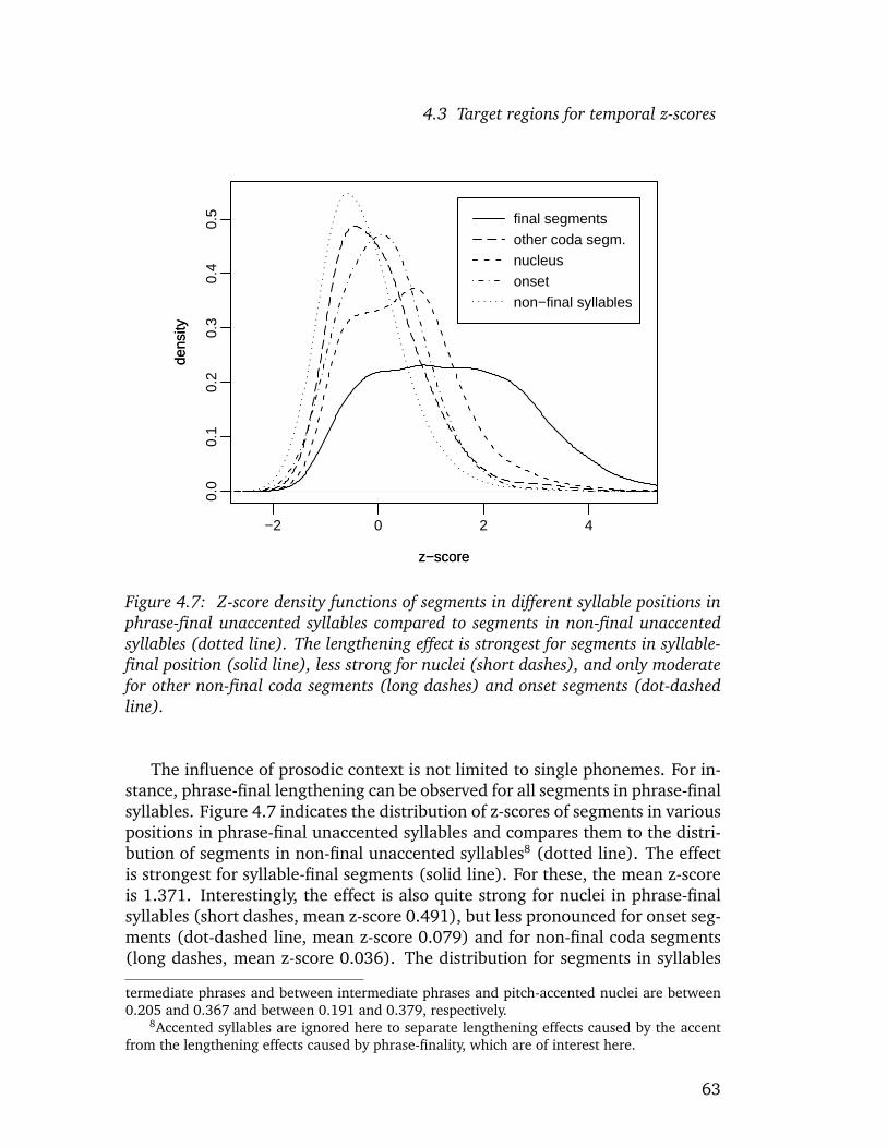
4.3 Target regions for temporal z-scores

−2 0 2 4

0.0

0.1

0.2

0.3

0.4

0.5

z−score

dens

ity

z−score

dens

ity

final segmentsother coda segm.nucleusonsetnon−final syllables

Figure 4.7: Z-score density functions of segments in different syllable positions inphrase-final unaccented syllables compared to segments in non-final unaccentedsyllables (dotted line). The lengthening effect is strongest for segments in syllable-final position (solid line), less strong for nuclei (short dashes), and only moderatefor other non-final coda segments (long dashes) and onset segments (dot-dashedline).

The influence of prosodic context is not limited to single phonemes. For in-stance, phrase-final lengthening can be observed for all segments in phrase-finalsyllables. Figure 4.7 indicates the distribution of z-scores of segments in variouspositions in phrase-final unaccented syllables and compares them to the distri-bution of segments in non-final unaccented syllables8 (dotted line). The effectis strongest for syllable-final segments (solid line). For these, the mean z-scoreis 1.371. Interestingly, the effect is also quite strong for nuclei in phrase-finalsyllables (short dashes, mean z-score 0.491), but less pronounced for onset seg-ments (dot-dashed line, mean z-score 0.079) and for non-final coda segments(long dashes, mean z-score 0.036). The distribution for segments in syllables

termediate phrases and between intermediate phrases and pitch-accented nuclei are between0.205 and 0.367 and between 0.191 and 0.379, respectively.

8Accented syllables are ignored here to separate lengthening effects caused by the accentfrom the lengthening effects caused by phrase-finality, which are of interest here.

63

4.3 Target regions for temporal z-scores

−2 −1 0 1 2 3 4

0.0

0.1

0.2

0.3

0.4

0.5

0.6

z−score

dens

ity

final segmentsother coda segm.nucleusonsetunacc. syllables

Figure 4.8: Z-score density functions of segments in different syllable positionsin non-final accented syllables compared to segments in non-final unaccented syl-lables (dotted line). The lengthening effect is present and similarly strong forsegments in syllable-final position (solid line), nuclei (short dashes), and onsetsegments (dot-dashed line). It is, however, not detectable for non-final coda seg-ments (long dashes).

which are not phrase-final at all (dotted line) is indicated for comparison (meanz-score -0.286). Four Wilcoxon rank sum tests reveal that the differences aresignificant except for onset segments vs. non-final coda segments (long dashesvs. dot-dashed line)9. However, these latter distributions are still significantlydifferent from the distribution of segments in non-phrase-final syllables (dottedline), confirming that the effects are detectable for all segments in phrase-finalsyllables.

Similarly, lengthening can be observed not only for accented nuclei, but forother segments in accented syllables. Figure 4.8 compares the z-score distribu-

9Calculation of the 99.9% confidence intervals for pairwise differences of the means revealsthat the true differences in means lie between 0.733 and 0.962 for syllable-final segments com-pared to nuclei, between 0.297 and 0.450 for nuclei compared to onset segments, and between0.188 and 0.372 for non-final coda segments compared to segments from non-final syllables.The difference between onset and non-final coda segments is not significant (p≈0.004).

64

4.3 Target regions for temporal z-scores

tions of segments in various positions in accented non-final syllables to the z-score distribution of segments in unaccented non-final syllables (dotted line)10.It can be seen that the effect is similarly strong for onset segments (dot-dashedline, mean z-score 0.358), nuclei (dashed line, mean z-score 0.253), and finalsegments (solid line 0.176). Wilcoxon rank sum tests reveal that there is nosignificant difference between the former two (p≈0.029), and a small but sig-nificant difference between the latter two11. There is, however, still a significantdifference between syllable-final segments in accented syllables (solid line) andsegments in unaccented syllables (dotted line)12. Interestingly, the effect is notpresent for non-final segments in the coda of accented syllables (long dashes),as there is no significant difference (p≈0.851) between their distribution andthe z-score distribution of segments in unaccented syllables (dotted line).

It is an astonishing finding that the strength of effect both in phrase-finallengthening and in lengthening related to pitch accents does not increase ordecrease monotonically in the course of a syllable. One could have expected forinstance that phrase-final lengthening increases towards the end of the phraseand is strongest for the very final segment in a phrase. Instead, figure 4.7suggests that the effect is present in the onset segments already, increases fornuclei, then decreases for interceding coda segments, before reaching the max-imum for the very final segment in the phrase. Similarly, one might have ex-pected that nuclei are affected the most by lengthening related to pitch accents,but it is interesting that the effect is similarly strong for the final segment in thesyllable, while it is not present at all for interceding coda segments. Theseobservations will be investigated further in future work.

The influence of prosodic context can also be seen in syllable-level z-scoredistributions. When examining z-scores of syllables, the problem arises thatsome syllables are extremely rare. For instance, 1,650 of altogether 3,863 syl-lable types occur only once in the MS corpus; 2,947 syllables types occur 5times or less, 3,322 types occur up to ten times. The smaller the number ofinstances of a particular syllable type, the less reliable is the z-score calculatedon that basis, particularly because it is likely that there are still some segmen-tation errors in a corpus of this size even after manual checking. Thereforeonly the z-scores of those 340 types were examined for which there are at least20 realizations in the corpus. These syllable types add up to 22,650 syllabletokens.

When looking at their z-score distributions, the same effects of prosodiccontext on the syllable level as on the segment level can be found. The dis-

10Phrase-final syllables are ignored here to separate phrase-final lengthening effects fromthe lengthening effects related to pitch accents, which are of interest here.

11Calculation of the 99.9% confidence interval for pairwise differences of the means yieldstrue differences between 0.019 and 0.127 for nuclei compared to syllable-final segments.

12The true difference between means lies between 0.432 and 0.499 with a confidence of99.9%.

65

4.3 Target regions for temporal z-scores

−4 −2 0 2 4 6 8

0.0

0.1

0.2

0.3

0.4

z−score

dens

ityall syllablesaccentedphrase final

Figure 4.9: Lengthening effects on the syllable level: Z-score density functions forall syllables (dotted line), accented syllables (dashed), and phrase-final syllables(solid). Z-scores of accented syllables and phrase-final syllables are significantlyhigher than the average.

tributions are depicted in figure 4.9. Syllable-level z-scores are higher thanaverage for pitch-accented syllables, and even higher for phrase-final syllables:the overall mean z-score is 0.000, while the means for pitch-accented syllablesand for phrase-final syllables are 0.611 and 1.174 respectively. The differencesin means are again highly significant13.

As for the difference between intonation phrases and intermediate phrasesobserved on the segmental level in figure 4.6, the effect is less obvious in figure4.9. There is only a very slight bump on the left slope of the distribution forphrase-final syllables. Nevertheless the underlying distributions of intermedi-ate and intonation phrases are still different, as illustrated by figure 4.10: thedistribution for phrase-final syllables (solid line) can be split up into interme-diate phrases (dot-dashed line) and intonation phrases (dashed line). Again,the distribution for all syllables is depicted as a reference (dotted line). Thebump is less obvious in this case because there is more overlap between thetwo distributions on the syllable level than on the segment level. Since there arealso more realizations of boundary tones than of intermediate phrase bound-aries, the peak corresponding to the maximum in the distribution for intonation

13Three pairwise Wilcoxon rank sum tests yield 99.9% confidence intervals for the differ-ences in means between 0.565 and 0.675 for all syllables as compared to pitch-accented sylla-bles, between 0.493 and 0.674 for accented syllables compared to phrase-final syllables, andbetween 1.134 and 1.274 for all syllables vs. phrase-final syllables.

66

4.3 Target regions for temporal z-scores

−2 0 2 4

0.0

0.1

0.2

0.3

0.4

0.5

syllable−level z−score

dens

ityall syllablesphrase finalipIP

Figure 4.10: Z-score density function for phrase-final syllables (solid line), re-peated from figure 4.9. The distributions of phrase-final syllables in intermediatephrases (ip, dot-dashed) and intonation phrases (IP, dashed) are significantly dif-ferent. For comparison, the z-score distribution for all syllables is again indicatedby the dotted line.

phrases is dominant even in the overall distribution for all phrase-final syllables.To summarize the experimental results presented in this section, it can be

stated that consistent effects of prosodic events on the duration z-scores havebeen observed both on the segment and on the syllable level. Different prosodiccontexts produce significantly different z-score distributions.

Under the assumption that the z-scores can be interpreted as a relevantdimension in the perception of prosody, the z-score distributions for differentprosodic events implicitly define overlapping, but significantly different targetregions: they identify the range of acceptable z-scores for each prosodic event.Likewise, Keating (1990) proposed that the range of observed values along adimension in production defines the window which serves as a target region forproduction.

Answering question (iii), which are the target regions corresponding tothese events, I conclude that the z-score distributions for speech units relatedto prosodic events implicitly define the temporal target regions in the produc-tion of these events. Turning again to the question of the nature of the speechunits—segments, syllables, or possibly higher-level units—I have shown thatprosodic effects are not only detectable in the z-score distributions of segmentsbut also in those of syllables, thus both segments and syllables may be the un-derlying units; however, I do not want to rule out that such effects could be

67

4.4 Temporal target regions and the syllabary

found on the word-level as well. The following section will shed more light onthis issue, suggesting that both the segment and the syllable levels may play arole, depending on the frequency of the speech unit that is to be produced.

4.4 Temporal target regions and the syllabary

Levelt’s model of speech production (Levelt 1992; Levelt and Wheeldon 1994;Levelt 1999) assumes that the basic unit in articulation is the syllable. Convinc-ing evidence for this claim came from results of implicit priming experimentsreported by Cholin et al. (2004). Levelt claims that gestural scores for thearticulation of syllables are stored in a mental syllabary. It is left open, how-ever, whether gestural scores for all syllables are stored, even for languages likeEnglish or Dutch, which are claimed to have approximately 12,000 syllables(Levelt 1999, p. 111), or whether scores for infrequent syllables are computedon-line. However Levelt notes that for English, 500 frequent syllable typeswould already cover 80% of the syllable tokens (Levelt 1999, p. 111), implicitlysuggesting that only these frequent syllables might be stored in the syllabary.

Similar figures can be found in the MS corpus, even though the corpus hasbeen designed to increase coverage of rare diphones. For instance, as men-tioned in section 4.3, the corpus contains 3,863 different syllable types. 1,650of them occur only once, but 588 syllables occur at least ten times each. These588 types add up to 25,978 tokens and make up almost 77% of the entire cor-pus. Reasoning as Levelt above, this might already be a sufficient proportion tobe stored in the syllabary. Moreover, the 1,650 syllables that occur only oncecan be said to be not only infrequent but extremely rare, considering that thecorpus consists of 160 minutes of speech, and has been optimized for coverage,i.e. infrequent units should be overrepresented compared to randomly selectedcorpora of the same size. I would maintain that the average speaker producessignificantly less than 160 minutes of speech per day, least of all with a vocabu-lary as diverse as that of the speech corpus investigated here. It is questionablewhether gestural scores of extremely rare syllables that a speaker produces, say,once in a week can be expected to be stored in memory.

In any case, according to Levelt (1999), what is stored in the syllabary isthe articulatory scores of syllables. In the sense of Guenther et al. (1998) andPerkell et al. (2000), however, these scores would be auditory rather than ar-ticulatory, and they can be thought of as trajectories through auditory targetregions for subsequent speech segments. These trajectories are only later trans-lated into motor commands by feed-forward mappings learned during speechacquisition (cf. section 2.2).

Assuming the exemplar-theoretic approach to target regions as outlined inthe preceding section 4.3, according to which target regions are implicitly de-fined by accumulations of exemplars, it naturally follows that very infrequent

68

4.4 Temporal target regions and the syllabary

syllables might indeed not be stored in the syllabary but have to be computedon-line instead: Infrequent units are represented by considerably fewer exem-plars; for the most infrequent units, there may be too few exemplars to qualifyas an “accumulation” of exemplars over which we can abstract. This impliesthat there might be no or no reliable target regions available for infrequentunits, and that the speaker has to resort to smaller and therefore more frequentunits. I will illustrate this using some concrete figures from the MS corpus inthe following section.

4.4.1 Frequent and infrequent syllables

In the MS corpus, the 340 most frequent syllable types, which occur, as men-tioned in section 4.3 above, at least 20 times each, account for 22,650 syllabletokens and thus cover approximately 67% of the corpus. These figures give animpression of the order of magnitude of exemplars possibly stored in memory.They confirm that at least for very frequent syllables, there must be enoughexemplars to be useful as a reference in speech production without resorting tothe segment level.

As for determining which are the very infrequent syllables, the frequenciesobserved in the MS corpus cannot be relied on. Instead the frequency classifica-tion of the syllables was based on syllable probabilities induced from multivari-ate clustering (Muller et al. 2000), which allows estimation of the theoreticalprobability even for unseen syllables. In Muller et al. (2000), probabilities wereobtained for a total of 41,711 German syllable types, ranging from 4.61*10-11

(for the syllable [R@sk]) to approximately 0.0259 (for the syllable [de:6]). TheMS corpus contains 3,793 syllable types, which means that there could be al-most 38,000 syllable types missing. Here the question arises how realistic thenumber of 41,711 is as an estimation of the number of different syllable types.It is worth noting that actually existing syllables can be found even among theleast probable ones. On the other hand, some of them seem very unlikely,such as the syllable [R@sk] mentioned above for instance, since the consonantcombination [sk] in the coda to my knowledge can only occur in the contextof stressed syllables in morpheme final position in non-native German words(with the exception of the native German word brusk, [brYsk]), and thereforeshould not occur in combination with the unstressed schwa [@], which usuallyonly occurs in native German words.

For comparison, Celex (Baayen et al. 1995) contains only approximately11,000 syllable types. But this is by no means the upper limit of different sylla-ble types in German. For instance, the MS corpus contains syllables occurringin existing words that are not listed in Celex. Also, more words are used inGerman than can be expected to be listed in such a dictionary. German propernames for instance contain many types that are not listed in Celex. For ex-

69

4.4 Temporal target regions and the syllabary

ample, according to a cliche, the most popular German surname is Schmidt,pronounced [SmIt], but [SmIt] as a syllable does not occur in Celex. The sylla-bles [ja:n] as in one possible pronunciation of Jan, [klaUs] as in Klaus, [jY6] asin Jurgen, all very frequent male first names, and the syllable [pOts], as in theGerman city Potsdam, are also missing. Other existing German syllables thatare not in Celex comprise clitizations (e.g. [dU6Cs] as in durchs, which resultsfrom appending the clitic ’s to the preposition durch, or [tsUm] as in zum, thepopular short form of zu dem) and inflectional forms not listed in Celex (suchas [hE6n] as in Herrn, the dative form of Herr). These are just some examples,more can be found easily. This leads me to conclude that realistically, there aremany more than 11,000 syllable types in German, with the upper limit beingapproximately 41,000. This means that the number of syllables missing fromthe corpus is somewhere between many more than 7,000 and 38,000.

Summing up these considerations, it can be said that there are many existingsyllable types that are not represented by even one token in a speech corpus of160 minutes of speech. It is therefore likely that for very infrequent syllables,there are not enough exemplars stored in memory to serve as a reference inspeech production, and that the respective segments must be used as targetsinstead.

4.4.2 Dual-route phonetic encoding

Assuming that not all syllables are stored in the syllabary but only the most fre-quent ones, it follows that gestural scores or trajectories through target regionshave to be computed on-line for the less frequent syllables. Then, two differentstrategies would be used by speakers when producing frequent vs. infrequentsyllables. This has been called dual-route phonetic encoding by Whiteside andVarley (1998a), with a direct route, and less computational demand, for fre-quent syllables, and an indirect route for infrequent syllables, which requireson-line computation of gestural scores.

Whiteside and Varley (1998a) hypothesize that the direct route encodingshould be characterized by “higher syllable cohesion” and therefore “increasedcoarticulation or gestural overlap” (Whiteside and Varley 1998a, p. 3155) (inaddition to shorter response latencies in production experiments). This hy-pothesis is supported by their view that in apraxia of speech “either the accessto and/or storage of verbo-motor patterns are disrupted” (Whiteside and Var-ley 1998b, p. 223), and that patients suffering from apraxia of speech, whowould then always have to use the indirect route, show indeed less coarticula-tion and inconsistent articulatory movements, among other things. They alsoclaim (Whiteside and Varley 1998a, p. 3155) that the indirect route is proba-bly used in careful speech, which again exhibits less coarticulation than normalspontaneous speech.

70

4.4 Temporal target regions and the syllabary

To substantiate their hypothesis, Whiteside and Varley (1998a) measure re-sponse latencies, utterance and word durations, and second formant frequencychanges of frequent vs. infrequent English words. However, significant effectsof word frequency are only confirmed for response latencies, supporting the hy-pothesis that different strategies are used in the production. As for the secondformant changes as a measure of coarticulation, the effect is not significant.This is attributed to the small sample size of only 30 tokens in each conditionand to inter-speaker variability.

Another reason for their failing to find significant differences other thanresponse latencies may be the fact that they control for word frequency ratherthan syllable frequency, although the model proposed by Levelt and Wheeldon(1994), upon which they base their hypothesis, assumes syllables as the unit ofarticulation and not words.

An experiment aiming at differences in the degree of coarticulation in syl-labary and non-syllabary syllables was conducted by Dogil, Ostry, and Schillerin 2000 (Dogil, personal communication) in an unpublished pilot study. Theydid find differences in the degree of coarticulation when looking at (labial) ar-ticulatory movements of syllables assumed to be in the syllabary vs. those ofnon-syllabary syllables. More precisely 12 two-syllable nonsense words, cover-ing the four possible combinations of English syllabary and non-syllabary sylla-bles, were embedded in an English carrier sentence and repeated 25 times eachby a native (Canadian) English speaker. The classification of syllables as belong-ing to the syllabary was based on syllable frequencies obtained from the BritishNational Corpus. For the non-syllabary syllables BST-ELITE lip tracings14 of the25 repetitions were more consistent than for the syllabary syllables, confirmingthat there was less coarticulation for the infrequent non-syllabary syllables.

4.4.3 The dual-route hypothesis in the temporal domain

With respect to temporal planning, the analogous assumption is that if, becauseof a lack of an appropriate syllable-level target, a very infrequent syllable is pro-duced by concatenating segments, then the z-score of the resulting realizationof the syllable should depend on the z-scores of the involved segments. Thereshould be less dependency for very frequent syllables, because then the speakerdoes not access exemplars of the involved segments but directly uses exemplarsof the syllable as a reference. For instance if a speaker intends to articulate asyllable lengthened by a z-score of 2, but does not have enough exemplars ofthe syllable to use as a reference, he will articulate the syllable using exemplarsof the involved segments with a z-score of 2. Consequently, more variation can

14Two-dimensional movements of two reflector points on the upper and lower lip of thespeaker are registered by two cameras, using a third reflector point on the nasion as a reference.The two camera tracings are combined to obtain a three-dimensional tracing.

71

4.4 Temporal target regions and the syllabary

be expected for frequent syllables than for infrequent syllables when looking atthe relationship between syllable z-scores and the z-scores of the correspondingsegments.

To assess the validity of the hypothesis, the specifics of the MS corpus can beexploited. Since the corpus was designed for unit selection synthesis (cf. section4.1), one objective was to have a good coverage even of phonemes in infrequentcontexts, and to have at least the same coverage as a diphone corpus. There-fore, after optimizing coverage for phoneme/context vectors, sentences con-taining diphone types that were not found in the corpus were manually added.As a consequence, the corpus differs from a randomly collected database in thatit exhibits an unusual syllable frequency distribution with disproportionatelymany instances of some otherwise infrequent syllables. This makes it possibleto compute z-scores for realizations of these syllables even though they shouldusually not be represented by a sufficient number of exemplars in a speaker’smemory for him to have established stable target regions.

To test the hypothesis, two linear regression models were calculated, onefor very frequent and one for very infrequent syllables. Both models predict thesyllable z-score from the mean z-score of the involved segments. The criterionfor identifying infrequent and frequent syllables was a probability of less than0.00005 according to Muller et al. (2000) for very infrequent syllables, and ofmore than 0.001 for very frequent syllables (cf. section 4.4.1).

To obtain reliable z-scores, only those syllables were taken into account forwhich there were more than 20 realizations in the MS corpus. Some of the mostfrequent syllables obviously came from frequent function words which usuallydo not carry pitch accents. To avoid overrating the effects of typical prosodiccontexts, such syllables were explicitly excluded, only taking types into accountfor which there was at least one instance carrying a pitch accent in the database.This left 108 very frequent and 16 very infrequent syllable types which met therequirements, adding up to 4,548 and 742 tokens, respectively. Figure 4.11shows the mean z-scores of involved segments plotted against syllable z-scoresfor frequent (left panel) and infrequent (right panel) syllables, together withthe regression lines.

For the two linear regression models, the residual standard errors were0.391 for frequent and 0.340 for infrequent syllables. This indicates that indeedthe model for frequent syllables is less accurate in predicting syllable z-scoresfrom mean segment z-scores, confirming that there is a stronger linear depen-dency between the two values for infrequent syllables. To determine whetherthis difference is significant, the Bartlett test for homogeneity of variances wasapplied to the residuals. The test confirmed that the variances are significantlydifferent (p�0.0001) and thus supports the hypothesis: There is a strongerrelationship between mean segment z-score and syllable z-score for infrequentthan for frequent syllables.

This result confirms that mean segment z-scores better predict the syllable

72

4.4 Temporal target regions and the syllabary

−2 −1 0 1 2 3 4 5

−2

02

46

z−score of syllable

mea

n z−

scor

e of

seg

men

ts

−2 −1 0 1 2 3 4 5

−2

02

46

z−score of syllablem

ean

z−sc

ore

of s

egm

ents

Figure 4.11: Mean z-scores of segments within a syllable plotted against z-score ofthe syllable for frequent (left panel) and infrequent (right panel) syllables.

z-score in the case of infrequent syllables. Note that the regression lines infigure 4.11 almost go through the origin and have a slope of approximately 1.This indicates that the mean segment z-scores in both cases not only predict thesyllable z-score; they are even almost equal to the syllable z-score. However,the residuals are slightly greater in the case of frequent syllables, indicatingthat there was more variation in the relationship between segment and sylla-ble z-score. Assuming that for frequent syllables, speakers establish a syllablez-score target, while for infrequent syllables, they establish a sequence of seg-ment z-score targets would predict this outcome. For the segment targets, thedurations of the constituent segments are given by the their z-scores. Morevariability is possible for syllable targets: here, only the z-score of the syllableis fixed, but there is no prescription how the duration should be distributed tothe constituent segments.

The Multilevel exemplar model (Walsh et al. 2010) described in section2.3.4 models production using such a dual-route approach. Specifically, it as-sumes that complete syllables (“units”) are used as targets in production if theiractivation exceeds a certain threshold. Since strength of activation depends onthe number of exemplars of that type, this will usually be the case for frequentsyllables. If the activation level is not high enough (for instance for lack of ex-emplars of that type), which will typically be the case for infrequent syllables,the syllable is instead produced using “constituent” segments as production tar-gets. Walsh et al. (2010) present a simulation experiment in which the modelis seeded with typical durations form the MS corpus used here. It then itera-tively produces syllables, adding the resulting syllables as exemplars after each

73

4.5 Conclusion

step. The model generates each syllable type n times, where n reflects the syl-lable’s prior probability, i.e, frequent syllables are produced more often thaninfrequent syllables. Thus, the number of frequent syllable exemplars at somepoint becomes sufficient to allow for unit level production, i.e., for using a syl-lable exemplar as production target rather than exemplars of its constituentsegments. The model obtained in this way then produces each syllable type500 times (without storing the resulting syllables to avoid compromising therelative frequencies of syllable exemplars in memory). The syllable and seg-ment durations generated that way exhibit the same behavior as the durationsin the MS corpus: in case of infrequent syllables, mean segment z-scores betterpredict the syllable z-score than in case of frequent syllables.

4.5 Conclusion

In this chapter I have presented an exemplar-theoretic interpretation of Guen-ther and Perkell’s speech production model (Guenther et al. 1998; Perkell etal. 2000) for the prosodic domain. I have suggested that z-scores of speechunit durations are the temporal dimension in the perception and productionof prosody. From an exemplar-theoretic perspective, the z-score of a speechunit can be interpreted as its position in the exemplar cloud with respect to theduration dimension. Assuming that speech units are stored including their du-rations, which is in accordance with the exemplar-theoretic models discussedin section 2.3, speakers and listeners have access to the position of exemplarsin the cloud and therefore to their temporal z-score.

The exact nature of the speech units is left open. Following Levelt (1999),I have assumed here that the basic unit in articulation is the syllable, and thatspeakers possibly have to resort to the segment level in the case of very infre-quent syllables, as suggested by the dual-route hypothesis discussed in 4.4.3.Experimental results from a large speech corpus seem to corroborate this view.However, only 16 infrequent syllable types were frequent enough in the cor-pus to be considered in the experiment, which is probably not enough to berepresentative of the large number of infrequent syllables. On the other hand,simulation results presented by Walsh et al. (2010) confirm the effect. They donot face the data sparsity problems because in the simulation, any infrequentsyllable can be produced as often as necessary. Still, I believe that carefully con-trolled production experiments would be valuable to add another methodologyof assessing differences in variability between frequent and infrequent speechunits.

In any case, I have suggested that temporal z-score distributions of speechunits related to prosodic events implicitly define target regions in the produc-tion of temporal properties of prosodic events. As stated in section 2.3.5, this issimilar to Keating’s (1990) assumption that target regions are implicitly defined

74

4.5 Conclusion

by the range of observed values along a dimension. I have presented experi-mental results confirming that the z-score distributions of segments and sylla-bles in different prosodic contexts are significantly different, i.e., from a theo-retical perspective, they could serve to distinguish between different prosodicevents. In other words, z-scores are an appropriate perceptual measure to makethe target regions for different prosodic events more distinct from each other.Of course, there is still a high amount of overlap between the distributions.Obviously, the temporal z-scores alone will not make the regions sufficientlydistinct from each other. I will turn to tonal aspects of prosody in the follow-ing chapter, and propose that when considering temporal and tonal dimensionstogether, the resulting multidimensional target regions may be sufficiently dis-tinct.

75

Chapter 5

The tonal dimension of perceptualspace

When turning to the tonal dimensions of the target regions of prosodic events,again three questions arise, just as for the temporal dimension discussed inchapter 4. These questions are, in analogy to the temporal domain: (i) what arethe tonal dimensions of perceptual space, (ii) which are the relevant prosodicevents, and (iii) which are the target regions corresponding to these events.

With regard to question (ii), as suggested in the introduction to chapter 4,I will assume for now that phrase boundaries and pitch accents according toGToBI(S) (Mayer 1995) are the relevant prosodic events. Since pitch accentsand boundary tones are defined as tonally distinct units, it is self-evident thatthey will differ with respect to their tonal properties.

I will suggest to answer question (i) in this chapter by proposing the PaIntEparameters introduced in chapter 3 as perceptually relevant tonal dimensions.To motivate the PaIntE parameters as the perceptually relevant tonal dimen-sions, I will explain how they capture relevant tonal properties of the pitchaccents and boundary tones of the GToBI(S) labeling system in section 5.1.

In analogy to the temporal domain discussed in chapter 4, I will then pro-pose to answer question (iii) by assuming that the distributions of PaIntE pa-rameters related to prosodic events can be regarded as target regions in theproduction and perception of tonal aspects of prosodic events, as explicated insection 5.2.

5.1 Interpretation of the PaIntE parameters

This section is intended to illustrate the relation between PaIntE parametersand the tonal implementation of pitch accent and boundary types. For four ofthe six parameters, I will explain which values of the parameters one wouldexpect for which accents and boundaries, and show how these expectations

76

5.1 Interpretation of the PaIntE parameters

Figure 5.1: Schematic of the PaIntE approximation function repeated from figure3.3.

are borne out using density plots of the parameter distributions of the differentaccent and boundary types found in the SWMS corpus.1,2 I will also contrasttheir parameter distributions with those of unaccented syllables. Although Iwill only use data from one male speaker here, the experiments described inchapter 6 will show that prosodic classifiers trained using, among others, thePaIntE parameters generalize well to a similar corpus of a female speaker, whichto some extent indicates that the tonal properties found in the PaIntE parameterdistributions of the SWMS corpus are not speaker-specific but reflect generalproperties of the German intonation system.

The PaIntE approximation and the resulting parameters have been discussedin section 3.2 already. The graphical display of an example pitch contour asspecified by the PaIntE parameters is repeated in figure 5.1. From the schemat-ics of the pitch accents of GToBI(S), which had been discussed in section 3.1,and which is repeated in figure 5.2, it can be seen that almost all accents in-volve some kind of peak (L*H, H*L, H*) or at least high plateau (HH*L) in thepitch contour, with the exception of completely linked L*, in which case onlythe left (”valley”) part of the contour given in figure 5.2 is realized. The peaks

1The SWMS corpus is described in some detail in section 6.1.2 because the exact specifi-cation is more important for the experiments presented in chapter 6 than it is here. Here, itsuffices to say that the corpus consists of approximately 2 hours of speech of a male speaker,that the speaker was the same as in the MS corpus used in chapter 4, and that the corpus wasoriginally recorded for unit selection speech synthesis.

2For the two remaining parameters, the expectations are less clear, and I will not discussthem here.

77

5.1 Interpretation of the PaIntE parameters

HH*L

syl sylacc. syl syl sylacc. syl

L*HL

syl

L*H

syl sylacc. syl

H*L

syl sylacc. syl

syl acc. syl

L* ..H

preacc. syl...

syl acc. syl

H* ..L

preacc. syl...

Figure 5.2: Schematic diagrams of the pitch contours of the GToBI(S) pitch ac-cents, repeated from section 3.1. Boxes represent syllables, accented syllables arehighlighted in gray color. Dotted lines indicate one or several interceding syllables.Dashed lines indicate that the actual contour arises from interpolation to targetsof preceding or following accents.

can be modeled by the peak of the PaIntE function.It may seem less promising at first glance to model L* using the PaIntE

function, but I have described in chapter 3 that for syllables for which no F0peak can be detected, the approximation is carried out using just the rising orjust the falling part of the PaIntE function for the approximation, i.e., using justone of the single sigmoids indicated by the dotted lines in figure 5.1. In thatcase, the b parameter still determines where that sigmoid reaches its maximum,i.e., it specifies where the rise comes to an end or where the fall starts, andthe corresponding c parameter (c1 for a rise, c2 for a fall) still represents theamplitude of the rise or fall. Thus, L* accents are expected to be modeled usingjust the rising sigmoid indicated as rising dotted line in figure 5.1. This maystill be suboptimal, because it does not explicitly model a valley, but the startof the rise should still correspond to the low target for L*. Also, at least in my

78

5.1 Interpretation of the PaIntE parameters

L*H H*L H* L*HL L* ..L HH*L ..H (L)% H% (H)− (H)% (L)−

3182

1820

767

26896 26 2 2

14281200

789

399

59

Figure 5.3: Histograms of pitch accent types (left panel) and boundary types (rightpanel) in the data used for the experiments presented in this chapter. The absolutenumbers for each type are plotted just above the corresponding bar.

experiments, the question of whether the modeling is adequate for L* or notwas of less importance because of the rarity of L* in our data (only 1.6% of thepitch accents in the SWMS corpus were L* accents).

For examining the PaIntE distributions of boundary tones, I have modifiedthe inventory of boundary tones to disambiguate between tonally unspecifiedboundaries (%,-) that are high and those that are low. As mentioned in section3.1, unspecified boundaries “inherit” their specification by way of spreading ofthe preceding trail tone. Therefore I differentiate between the following into-nation phrase boundaries: (H)% boundaries, which are high because the pre-ceding high trail tone is spread, H% boundaries, which are high inherently, and(L)% boundaries, which inherit the specification as low from the preceding lowtrail tone3. Analogously, for intermediate phrase boundaries, I distinguish be-tween (H)- boundaries, which occur after high trail tones, and (L)- boundaries,which occur after low trail tones.

As for the frequencies of the prosodic events in the part of the SWMS corpusthat I will be using in this chapter for illustrating the relation between PaIntEparameters and pitch accent and boundary types, there were approximately6,200 pitch accents and 3,900 boundaries. Figure 5.3 shows a histogram ofthe pitch accent types and their frequencies. It can be seen that some of thepitch accents were quite rare in the data: L* occurs only 96 times, and HH*L

3Inherently low L% boundaries were not labeled in the data of this particular speaker be-cause almost all full phrase boundaries are glottalized in his case, so that it was not possible toconsistently distinguish between L% and low unspecified % boundaries.

79

5.1 Interpretation of the PaIntE parameters

occurs only twice. The linked trail tones ..L and ..H are also very infrequent,with only 26 and 2 occurrences, respectively. As for phrase boundaries, lowintermediate phrase boundaries (L)- are also not frequent, with only 59 occur-rences. Since I am going to examine the parametrization results by interpretingplots of estimated probability distributions (also referred to as “density plots”in the following),4 I will for the sake of reliability only discuss the results ofthose prosodic events that are represented by at least 200 tokens. This leavesthe four most frequent accents L*H, H*L, H*, and L*HL, as well as H%, (H)%,(L)%, and (H)-. I will also compare the probability distributions of the pitch-accented syllables with those of unaccented syllables, and those of phrase-finalsyllables with those of non-final syllables.

5.1.1 Peak alignment

As stated above, the peak of the PaIntE function corresponds to the peak thatmost pitch accents exhibit. Its alignment with the syllable structure is deter-mined by the b parameter. If b is between 0 and 1, the peak is on the accentedsyllable. This is what one would expect for all accents that involve an H*, i.e.,all accents that have a high target on the accented syllable. However, in theHH*L case, the peak could be realized almost as a plateau, with similar pitchacross both the pre-accented and the accented syllable, giving rise to b valuesanywhere between -1 and 1, i.e., the peak will be either on the pre-accentedsyllable which is associated with the high target for the leading tone, or on theaccented syllable associated with the high target for the starred tone, depend-ing on which of the two syllables is realized with (possibly only slightly) higherpitch.5 For values of b greater than 1, the peak is on the post-accented syllableor later. This should be the case for L*H and L*HL, where the trail tone causesa high target in the pitch contour.

Figure 5.4 shows density plots of the b parameter. Generally, in densityplots, peaks appear at values that are more likely to occur for the underlyingsample, whereas valleys appear at values that are less likely to occur. Thedensity plots for different accent types can be compared because the densityfunctions are normalized so that the area below the line is equal to 1. Thus,for instance, if the plots for two different pitch accent types have equally highpeaks for a particular value of b, it can be inferred that for both accents, thatparticular value of b is equally likely. It can not be inferred, however, that giventhat particular value of b, the two accent types are equally likely, because of the

4All density plots were generated using the density function implemented in R (R Develop-ment Core Team 2009), which computes kernel density estimates for a sample of a populationin order to estimate the probability distribution of the entire population.

5There are only two instances of HH*L in the SWMS database. For these, the expectationis confirmed by values of approx. -0.3 and 0.4, respectively. Distributions of HH*L accents willnot be discussed in the following because of the sparsity of instances of this accent type.

80

5.1 Interpretation of the PaIntE parameters

0.0

0.2

0.4

0.6

0.8

1.0

1.2

1.4

Den

sity

−1syl

0syl

1syl

2

H*LL*HH*L*HLNONE

Figure 5.4: Density plots of the b parameter for the most frequent accents and forunaccented syllables. The syllable for which the approximation was carried out ishighlighted in gray. H*L accents (blue, long-dashed line) have their peak earlierin the accented syllable than H* accents (orange, dashed line) and L*HL accents(red, dot-dashed line). L*H accents (green, solid line) have their peak either on theaccented or on the post-accented syllable. For unaccented syllables (black, dottedline) peaks are detected on any of the three syllables of the analysis window.

differences in absolute frequencies of the accent types themselves.The density plots for the b parameter in figure 5.4 show that the above ex-

pectations are borne out. The vertical lines indicate syllable boundaries. Themiddle syllable, which is highlighted in gray, is the syllable for which the ap-proximation was carried out. In the distributions for pitch-accented syllables,this is the syllable associated with the accent. The blue, long-dashed line repre-sents the probability distribution for H*L accents. The relatively broad peak inthe middle of the accented syllable confirms that H*L accents have their peaksomewhere in the course of the accented syllable, but not at the very beginning.

81

5.1 Interpretation of the PaIntE parameters

The peak is roughly between 0.3 and 0.8. I will discuss H*L accents in moredetail below (cf. figure 5.6).

It can further be verified in this figure that H* accents, which are representedby the dashed orange line, also have their peak on the accented syllable; it isinteresting, however, that for H* accents, the peak is more likely to be laterin that syllable than for H*L accents.6 The peak is also a little more narrow,indicating less variation of b for H* accents than for H*L accents.

For L*HL accents, which are indicated by the red, dot-dashed line, surpris-ingly, the peak is also on the accented syllable. From the description of L*HLaccents given in section 3.1, one would expect that peak to be on the post-accented syllable. Still, compared to H*L and H*, the peak for L*HL accentsis shifted further towards the syllable boundary. It is also a little more nar-row than the two peaks of the H*L and H* distributions, indicating even lessvariation of b for L*HL accents.

Finally, the density for L*H accents (solid green line) is bimodal: L*H ac-cents are almost equally likely to have their peak either right before the syllableboundary, just as L*HL accents did, or to have their peak in the later part ofthe post-accented syllable. One might interpret this as evidence for two distinctcategories L+H* (with the peak on the accented syllable) and L*+H (withthe peak on the post-accented syllable) as in the Saarbrucken dialect of GToBI(Grice and Baumann 2002; Grice et al. 2005); however, it turns out that L*His realized differently on word-final syllables than on non-final syllables,7 asdemonstrated in figure 5.5. Here, the dashed line represents L*H accents thatoccurred on word-final syllables, and the dot-dashed line represents L*H ac-cents that occurred on word-internal syllables. Obviously, these two contextscause the bimodal distribution: L*H accents on word-final syllables almost al-ways have their peak in the accented syllable, while word-internal L*H accentstend to have their peak on the post-accented syllable. In other words, the tonalmovement on L*H accents usually does not cross word boundaries, instead it istimed to occur earlier before word boundaries.

As for the difference between accented and unaccented syllables, it is ob-vious from figure 5.4 that unaccented syllables (black, dotted line) vary muchmore in where the peak is detected. This is because peaks on unaccented sylla-bles are often due to microprosodic variation in pitch rather than to consciouspitch movements and are thus almost equally likely to occur on any of the sur-rounding syllables. I claim that the reason why they are discovered a little moreoften on the middle syllable is that this is the place where the algorithm startsto look for a maximum in the implementation of the PaIntE approximation(cf. section 3.2.3).

Altogether, figures 5.4 and 5.5 show that peaks for H*L accents usually oc-

6All distributions will be compared using confidence tests at the end of this section.7Thanks to Jorg Mayer for pointing me in the right direction.

82

5.1 Interpretation of the PaIntE parameters

0.0

0.5

1.0

1.5

Den

sity

−1syl

0syl

1syl

2

allfinalnonfinal

Figure 5.5: Density plots of the b parameter for L*H accents in different contexts.The accented syllable, for which the approximation was carried out, is highlightedin gray. The bimodal distribution for all L*H accents (solid line, repeated fromfigure 5.4) obviously arises from the fact that L*H accents in word-final syllables(dashed line) have their peak on the accented syllable, and L*H accents in word-internal syllables (dot-dashed line) have their peak on the following syllable.

cur earlier in the accented syllables than for H*, peaks for H* accents occurearlier than peaks for L*HL accents and word-final L*H accents, and that word-internal L*H accents have their peak on the post-accented syllable. Since thedistributions overlap, the accent types can not generally be inferred from thevalue of the b parameter alone. Such an inference may be valid for peaks thatoccur on the pre-accented syllable: in this case, it is very likely that the syllableis unaccented. This is because it is very unlikely for the pitch accents discussedabove to have their peak on the pre-accented syllable, but not unlikely at allfor unaccented syllables, and because, in addition, unaccented syllables are ingeneral more likely than accented syllables because of their dominance in fre-

83

5.1 Interpretation of the PaIntE parameters

0.0

0.2

0.4

0.6

0.8

1.0

Den

sity

−1syl

0syl

1syl

2

highmidlow

Figure 5.6: Density plots and mean values (vertical lines) of the b parameter inH*L accented syllables with low (dotted lines), mid (dashed lines), and high vowels(solid lines).

quency.Another interesting fact that can be observed in figure 5.4 is that peaks

are generally unlikely at the beginning of any syllable. This is in line withHouse’s (1996) model of optimal tonal perception, which claims that tonalmovements through areas of maximum new spectral information and inten-sity change (such as syllable onsets) are perceived as level tones rather than astonal movements. The model states that gestures of tonal movement must besynchronized to occur after these areas in order to be perceived as such. Thevalleys occurring in the density plots in figure 5.4 for all pitch accent types andall syllable onsets confirm that our speaker avoided placing peaks (and thus,placing the beginning of the falling tonal movement) in the spectrally unstableonsets.

Returning to H*L accents, Jilka and Mobius (2007) observed using the MS

84

5.1 Interpretation of the PaIntE parameters

corpus (cf. section 4.1) that peak alignment in H*L accents depends on theheight of the vowel in the accented syllable. They report that the point in theaccented syllable where the maximal F0 value is reached is later for highervowels: for low, mid, and high vowels, the maxima occur at 30.9%, 34.5% and41.8% of the voiced part of the syllable, respectively (median values). Theyused pairwise t-tests to confirm that the alignment for the three vowel heightsdiffer significantly, with p<0.001 when comparing high with non-high vowels,and p<0.005 when comparing mid vs. low vowels. The distributions of theb parameter observed here for the three cases confirm these differences. Forhigh vs. low vowels, they are significantly different8 with p<0.001; for highvs. mid vowels, they are significantly different with p<0.01, and for mid vs.low vowels, the difference is marginally significant (p<0.05). The means of bare 0.37 for low vowels, 0.48 for mid vowels, and 0.52 for high vowels. Thedistributions and the means are depicted in figure 5.6. The effect is significantin two of the three cases, but very subtle: the means, which are indicated bythe vertical lines, are very close, in particular for mid vs. high vowels, eventhough the difference was significant with p<0.01.

Turning to phrase boundaries, there are systematic differences between theprobability distributions of the b parameter for different boundary tones. Figure5.7 shows the density plots for the most frequent boundary types. Here, foursyllables are shown instead of just the three syllables in the analysis window,because in the case of low boundaries, the peak was sometimes found to beto the left, on the syllable just outside the window, i.e., two syllables beforethe actual phrase boundary. Therefore, the preceding syllable was included inthe plot, and thus the penultimate syllable in figure 5.7, which is highlighted ingray, is the syllable that has been analyzed. In the distributions for the boundarytones, this is the phrase-final syllable.

For the high boundaries, viz. H% (blue, long-dashed line), (H)% (red,dashed line), and (H)- (orange, dot-dashed line), peaks are almost always de-tected late in the final syllable. However, the detected peaks only indirectlycorrespond to production targets: On the phrase-final syllable, the pitch con-tour ends at a high level in the speaker’s register. The next syllable belongs tothe next phrase and therefore is usually produced at a lower level. This doescause a peak in the contour, because of the subsequent drop in F0. But onewould probably not want to interpret this drop in F0 as an intentional fallingtonal movement, rather, one would assume two underlying targets: the rise tothe high boundary, and, subsequently, a new, lower target for the next syllable.

Still, the PaIntE parameters capture valid, if not in every case intentional, F0movements occurring at phrase boundaries. For instance, the distribution forH% boundaries shows that their peaks tend to occur even later in the phrase-

8All statistical tests reported in this chapter have been conducted using the R statisticspackage (R Development Core Team 2009).

85

5.1 Interpretation of the PaIntE parameters

0.0

0.5

1.0

1.5

2.0

Den

sity

−2syl

−1syl

0syl

1syl

2

H%(H)%(L)%(H)−NONE

Figure 5.7: Density plots of the b parameter for the most frequent boundary typesand for non-final syllables. The syllable for which the approximation was carriedout is highlighted in gray. For high boundaries (H%, blue, long-dashed line; (H)%,red, dashed line; (H)-, orange, dot-dashed line) peaks are usually detected late inthe phrase-final syllable. For (L)% (green, solid line) there is a peak either on thephrase-final syllable or on the preceding syllables but almost never on the followingsyllable. For non-final syllables (black, dotted line), peaks are detected on any ofthe three syllables in the analysis window.

final syllable than those for (H)% and (H)- boundaries. This is because H%boundaries are expected to exhibit a contour that is rising throughout the sylla-ble and thus the maximum will be reached later; (H)% and (H)- boundaries, onthe other hand, are expected to be associated with a level contour on the finalsyllable, thus the exact location where the peak is detected is to some extentsubject to slight random variations in pitch on that syllable, as confirmed bythe broader and slightly earlier peaks in the corresponding probability distribu-tions.

86

5.1 Interpretation of the PaIntE parameters

Turning back to figure 5.7, the density plot for non-final syllables (dotted,black line) is depicted as well. As in the case of unaccented syllables discussedabove (cf. figure 5.4), peaks are likely to be detected on any of the three syl-lables, with a preference for the middle syllable, but again, I claim that this isdue to the fact that PaIntE starts to look for a maximum in the middle of thatsyllable.

(L)% phrase boundaries, finally, are usually found to have a peak in one ofthe preceding syllables. Their distribution is indicated by the green, solid linein figure 5.7. For (L)% boundaries, peaks are usually detected on either thefinal syllable or on the preceding one, which can be seen from the prevalenceof values between -1 and 0.5. Occasionally the peak is even on the syllablebefore that, with values of b between -2 and -1. The peak is found on precedingsyllables if there is no clear local maximum on the final syllable itself, but onone of the preceding syllables. This may be due to microprosodic variation, orto other prosodic events associated with these syllables. It can be noted herethat if the peak is on the final syllable, it is early in the syllable, which is in linewith the expectation that the tonal movement on that final syllable should befalling, making the location of a peak in the later part of the syllable unlikely.What is at first surprising, however, is that the peak is never detected on thefollowing syllable: there are virtually no values of b greater than 1 in the caseof (L)% boundaries. This is because in almost all cases of (L)% boundaries(96.4%), there is a silence following. Since the F0 contour is not interpolatedacross silences, there is a stretch of the speech signal for which no F0 values arepresent, and in these cases, the approximation window ends before that stretch.Thus, in almost all cases of (L)% boundaries, values of greater than 1 for b areless likely because the approximation is carried out in a window that ends onthe syllable associated with (L)%. These values can only arise if the contouris best approximated by a PaIntE function which reaches its peak outside thewindow, which does not happen often, but is theoretically allowed if b is notmore than half the window length beyond the window’s end (cf. section 3.2.4).Also, in many cases, (L)% boundaries are utterance-final, so often there is nofollowing syllable at all.

To conclude discussing the b parameter distributions, it is obvious that the bparameter captures meaningful aspects of peak alignment: the tendencies ex-pected based on the phonetic description of the GToBI(S) events are present inthe distributions. Also, effects observed by House (1996) and Jilka and Mobius(2007) can be found. It is also evident that the distributions for different typesare usually different, even though the differences in some cases are subtle.For both accents and boundaries, pairwise Wilcoxon rank sum tests reveal thatthe differences in most cases are significant. Table 5.1 lists the correspondingp-values, rounded to 5 digits. Values of 0.00000 indicate that p�0.000005. Al-

87

5.1 Interpretation of the PaIntE parameters

NONE H*L H* L*H L*HLNONE – 0.05808 0.00000 0.00000 0.00000H*L 0.05808 – 0.00000 0.00000 0.00000H* 0.00000 0.00000 – 0.00000 0.00000L*H 0.00000 0.00000 0.00000 – 0.00000L*HL 0.00000 0.00000 0.00000 0.00000 –

NONE H % (H)% (H)- (L)%NONE – 0.00000 0.00007 0.00000 0.00000H% 0.00000 – 0.00072 0.00000 0.00000(H)% 0.00007 0.00072 – 0.56745 0.00000(H)- 0.00000 0.00000 0.56745 – 0.00000(L)% 0.00000 0.00000 0.00000 0.00000 –

Table 5.1: p-values obtained by pairwise Wilcoxon rank sum tests comparing dis-tributions of b for the most frequent accent types (upper panel) and boundarytypes (lower panel). The distributions for unaccented syllables (NONE) vs. H*Laccents and those for (H)% vs. (H)- boundaries are not significantly different at aconfidence level of 0.999; all other distributions are significantly different. Valuesof 0.00000 indicate that p�0.000005.

most all distributions are significantly different at a confidence level of 0.999.9

Exceptions are the distributions of unaccented syllables (NONE) vs. H*L ac-cented syllables, and those of (H)% vs. (H)- boundaries.

5.1.2 Peak height

Parameter d of the PaIntE function determines the absolute height of the F0peak in Hz. Again, the distributions differ between accent types and betweenaccented vs. unaccented syllables. Density plots for parameter d are given infigure 5.8. Again, the distributions differ between accent types and betweenaccented vs. unaccented syllables. Values for d in Hertz are indicated on the xaxis: values to the right indicate higher peaks.

Figure 5.8 shows that syllables associated with H*L accents (blue, long-dashed line) and unaccented syllables (black, dotted line) exhibit the lowestvalues for d, i.e., their peaks are lower than peaks associated with the otheraccent types. In both cases, the peak in the distribution and thus the mostlikely value for F0 peak height is between 115 and 120 Hertz. In the case of

9This unusually high confidence level had been suggested in the preceding chapter in exam-ining the duration z-score distributions of the GToBI(S) events to make up for the high numberof confidence tests.

88

5.1 Interpretation of the PaIntE parameters

100 150 200 250

0.00

00.

010

0.02

00.

030

F0 [Hz]

Den

sity

H*LL*HH*L*HLNONE

Figure 5.8: Density plots of the d parameter for the most frequent accents andfor unaccented syllables. H*L accents (blue, long-dashed line) and unaccentedsyllables (black, dotted line) exhibit the lowest values for d; H* accents (orange,dashed line), L*HL accents (red, dot-dashed line), and L*H accents (green, solidline) are characterized by higher and more variable values for d.

H*L accents, I claim that this is due to the prevalence of nuclear, i.e., phrase-final, H*L accents over pre-nuclear H*L accents: 93% of the H*L accents arenuclear accents. For nuclear accents, I would expect lower peaks because ofthe declination. Indeed, the density plot for nuclear H*L accents only (notdepicted here) looks almost identical to the one for H*L accents depicted here,with the exception that the peak in the distribution is a little more narrowbecause nuclear H*L accents are even more likely to have their F0 peak atthat location. The density plot for non-nuclear H*L accents however (also notdepicted here) is shifted to the right and broader, very similar to the distributionfor L*H accents.

In the case of unaccented syllables, the dominance of lower peak heights

89

5.1 Interpretation of the PaIntE parameters

arises because peaks on unaccented syllables are often due to microprosodicvariation and will thus exhibit very little rise and fall amplitudes (cf. section5.1.3), so absolute peak heights depend more on where in the pitch range ofthe speaker the contour happens to be at that particular syllable than on theamplitude of the associated rise or fall. Thus, what is interpreted as a peak inthe PaIntE approximation is often just a very local small “bump” rather thana real “peak”, and one should probably speak of F0 maxima rather than ofF0 peaks in these cases. So, although unaccented syllables most often exhibitF0 maxima of around 115 to 120 Hertz, there is more variation than for H*Laccented syllables: higher F0 maxima are also possible, which can be seen fromthe broader shape of the distribution: values of up to 160 or 180 Hertz are notunlikely.

Figure 5.8 further demonstrates that peaks related to H* accents (orange,dashed line) are usually higher than those of H*L accents (blue, long-dashedline), which would follow, reasoning as above, from the fact that H* accentsare always pre-nuclear accents and thus are expected to exhibit higher peaksthan nuclear H*L accents because the declination effect is less strong for themthan for nuclear H*L accents. Peaks of L*HL accents (red, dot-dashed line) arehigher than those for H* (orange, dashed line), H*L (blue, long-dashed line) orunaccented syllables (black, dotted line). Since L*HL accents are claimed to beusually quite prominent and associated with greater amplitudes of rise and fall,this does not come as a surprise. Peaks of L*HL accents are higher even thoughthey are usually nuclear accents in our data (84%).

The distribution for L*H accents (green, solid line) is very similar to thatof L*HL accents (red, dot-dashed line), although there is again more variationfor L*H accents. Figure 5.9 demonstrates an interesting observation: the effectof phrase-finality observed above for H*L accents is reversed for L*H accents:60% of them are nuclear accents, i.e., they occur in phrase-final position, butcompared to the overall distribution for L*H accents (green, solid line, repeatedhere from figure 5.8) their distribution (red long-dashed line) is shifted even alittle more to the right, with the most likely value for peak height at around 150Hertz, i.e., nuclear L*H accents tend to have a higher peak than non-nuclearL*H accents. For non-nuclear L*H accents, the effect is similar to that for H*Laccents: the more accents follow an L*H within the same phrase, the higher thepeak, or, in other words, the earlier in the phrase, the higher the peak: peaksare typically realized at 125 to 130 Hertz for L*H accents that are followed byonly one more accent in the same phrase (blue, dashed line), at around 135Hertz for L*H accents that are followed by exactly two more accents (black,dot-dashed line), and at around 145 Hertz for L*H accents that are followed byexactly three more accents (orange, dotted line).

Concerning nuclear L*H accents, they could exhibit higher peaks if theyoccur immediately before phrase boundaries, because then the boundary couldreinforce the pitch movement associated with the L*H accent. Further analysis

90

5.1 Interpretation of the PaIntE parameters

100 150 200

0.00

00.

005

0.01

00.

015

0.02

0

F0 [Hz]

Den

sity

all L*Hnuclear L*H1 foll. acc.2 foll. acc.3 foll. acc.

Figure 5.9: Density plots of the d parameter for L*H accents in different positionsin the phrase. Compared to L*H accents in general (green, solid line, repeatedfrom figure 5.8), nuclear (i.e., phrase-final) L*H accents (red, long-dashed line)exhibit slightly higher values for d. For non-nuclear L*H accents, their position inthe phrase seems to have an effect on the d parameter: L*H accents with only onemore accent following in the same phrase (blue, dashed line) tend to have lowerd values than L*H accents with two accents following (black, dot-dashed line),which tend to have lower d values than L*H accents with three accents following(orange, dotted line).

reveals that this seems to be the case, but only to some extent: when lookingat L*H accents for which the phrase boundary does not immediately follow(i.e., not on the syllable itself, and not on the following one), the distribution(not depicted here) is shifted to the left and more narrow, i.e., if the boundarydoes not immediately follow, lower peak heights are observed, as expected.However, the peak of the distribution is still to the right of the one observedfor pre-nuclear L*H with only one accent following, i.e., peak height is still not

91

5.1 Interpretation of the PaIntE parameters

100 150 200 250 300

0.00

00.

005

0.01

00.

015

0.02

00.

025

F0 [Hz]

Den

sity

H%(H)%(L)%(H)−NONE

Figure 5.10: Density plots of the d parameter for the most frequent boundarytypes and for non-final syllables. Low boundaries ((L)%, green, solid line) exhibitslow values for d, while high boundaries (H%, blue, long-dashed line; (H)%, red,dashed line; (H)-, orange, dot-dashed line) are characterized by higher values.The d values for non-final syllables (black, dotted line) are in between.

ordered according to the position of the L*H in the phrase, even when excludingsyllables immediately before the phrase boundary.

Considering phrase boundaries, the d parameter also captures differences inthe distributions of the boundary types.: Figure 5.10 confirms that low bound-aries exhibit values that differ very clearly from those of high boundaries: Thedensity plot for (L)% boundaries, which is given by the green solid line, docu-ments a preference for relatively low values of d of around 100 Hertz, as wouldbe expected, while (H)% and (H)- boundaries, whose probability distributionsfor d are indicated by the red dashed and the orange dot-dashed lines, respec-tively, typically exhibit higher d values of around 150 Hertz. Non-final syllables(black dotted line) are somewhere in between, with d mostly between 110 and

92

5.1 Interpretation of the PaIntE parameters

NONE H*L H* L*H L*HLNONE – 0.00000 0.00000 0.00000 0.00000H*L 0.00000 – 0.00000 0.00000 0.00000H* 0.00000 0.00000 – 0.00000 0.0000L*H 0.00000 0.00000 0.00000 – 0.92136L*HL 0.00000 0.00000 0.00000 0.92136 –

NONE H % (H)% (H)- (L)%NONE – 0.00000 0.00000 0.00000 0.00000H% 0.00000 – 0.00000 0.00000 0.00000(H)% 0.00000 0.00000 – 0.58325 0.00000(H)- 0.00000 0.00000 0.58325 – 0.00000(L)% 0.00000 0.00000 0.00000 0.00000 –

Table 5.2: p-values obtained by pairwise Wilcoxon rank sum tests comparing dis-tributions of d for the most frequent accent types. The distributions for L*H andL*HL accents and those of (H)% and (H)- boundaries are not significantly differ-ent; all other distributions are significantly different at a confidence level of 0.999.Values of 0.00000 indicate that p�0.000005.

150 Hertz, while H% boundaries, as could be expected, are realized with thehighest pitch: their density plot (blue long-dashed line) has its peak at between170 and 180 Hertz.

In concluding the discussion of the d parameter, it can be said that the dis-tributions of this parameter confirm what could be expected from the phoneticdescription of the accents and boundary tones. Furthermore, there are clear dif-ferences in the distributions for different accent and boundary types. Wilcoxonrank sum tests confirm that all distributions are pairwise significantly differentat a confidence level of 0.999, with the exception of L*H vs. L*HL accents, andof (H)% vs. (H)- boundaries, for which the distributions are not significantlydifferent. Table 5.2 lists the p-values, rounded to 5 digits after the decimalpoint. Values of 0.00000 indicate that p�0.000005.

5.1.3 Amplitudes of rise and fall

Parameters c1 and c2 determine the amplitude of the rise towards the peak(c1) and the amplitude of the fall after the peak (c2) in Hertz. As mentionedin chapter 3, before approximating the F0 contour, PaIntE looks for a localmaximum in the contour. If such a maximum is found, the approximation iscarried out using the actual PaIntE function, which is the sum of a rising and afalling sigmoid. If no such maximum is found, the approximation is carried out

93

5.1 Interpretation of the PaIntE parameters

using only the rising sigmoid for rising contours, and only the falling sigmoidfor falling contours. In these cases, the c parameter that is undefined since itis not part of the term of the approximation function is set to 0. When usingthe actual PaIntE function with both sigmoids, values of 0 for either c1 or c2 donot arise. Thus, in the following plots, values of 0 mean that the parameter wasundefined originally. However, since it can be deduced in these cases that the F0contour can be best described as only a fall or only a rise, it is straightforwardto interpret the amplitude of the opposite, “non-existing”, movement as zero.

Figure 5.11 shows the distributions of c1 (upper panel) and c2 (lower panel)for different accent types. Looking at H*L accents first, which are indicated bythe blue long-dashed line, there is little surprise. It is obvious that they tendto have low values of c1, but higher values of c2: their c1 distribution showsa pronounced peak for c1 values of around 0 to 10 Hertz, and although thedistribution extends to the left with values of c1 up to 60 to 80 Hertz, the highervalues are much less likely. Their c2 distribution, on the other hand, shows aclear dominance of moderately high c2 values with values of around 0 beingrather unlikely. There is a broad peak between 20 and 40 Hertz, indicating thatthese are typical values of c2 for H*L accents. In short, H*L accents have smallrise amplitudes but higher fall amplitudes, as expected for falling accents.

L*H accents (green solid line) show just the opposite behavior: their c1values are typically between 20 and 60 Hertz, while their c2 values tend to beclose to 0, as one would expect for rising accents. The distributions for L*HLaccents are given by the red dot-dashed lines. They exhibit higher values forboth c1 and c2, reflecting their characterization as rise-fall accents.

H* accents should tend to have lower c1 and c2 values. These values shouldbe greater than 0, since H* accents should exhibit a small peak, and they shouldbe lower than the values observed for L*HL accents, since they do not neces-sarily involve pronounced falls or rises; rather, the course of the pitch contourdepends on the preceding and following targets. These expectations are con-firmed by the density plots for H* accents (orange dashed lines) in figure 5.11.

Unaccented syllables, which are represented by black dotted lines in bothpanels, tend to have c1 and c2 values close or equal to 0. This confirms thatunaccented syllables usually do not exhibit significant F0 rises or falls. However,this is just a tendency, not an absolute rule, as can be seen from the fact thatboth distributions have non-zero densities for higher c1 or c2 values. In thecase of unaccented syllables, I claim that these higher values for c1 or c2 canarise either (i) because of pitch accents or boundaries in the vicinity, in whichcase interpolation to tonal targets on adjacent syllables causes the F0 contourto rise or fall on the unaccented syllables themselves, or (ii) from the fact thattonal movements caused by accents associated with surrounding syllables arecaptured in the PaIntE parametrization. Figure 5.12 serves to illustrate thesetwo causes.

The black dotted line in figure Figure 5.12 indicates the distribution of c1

94

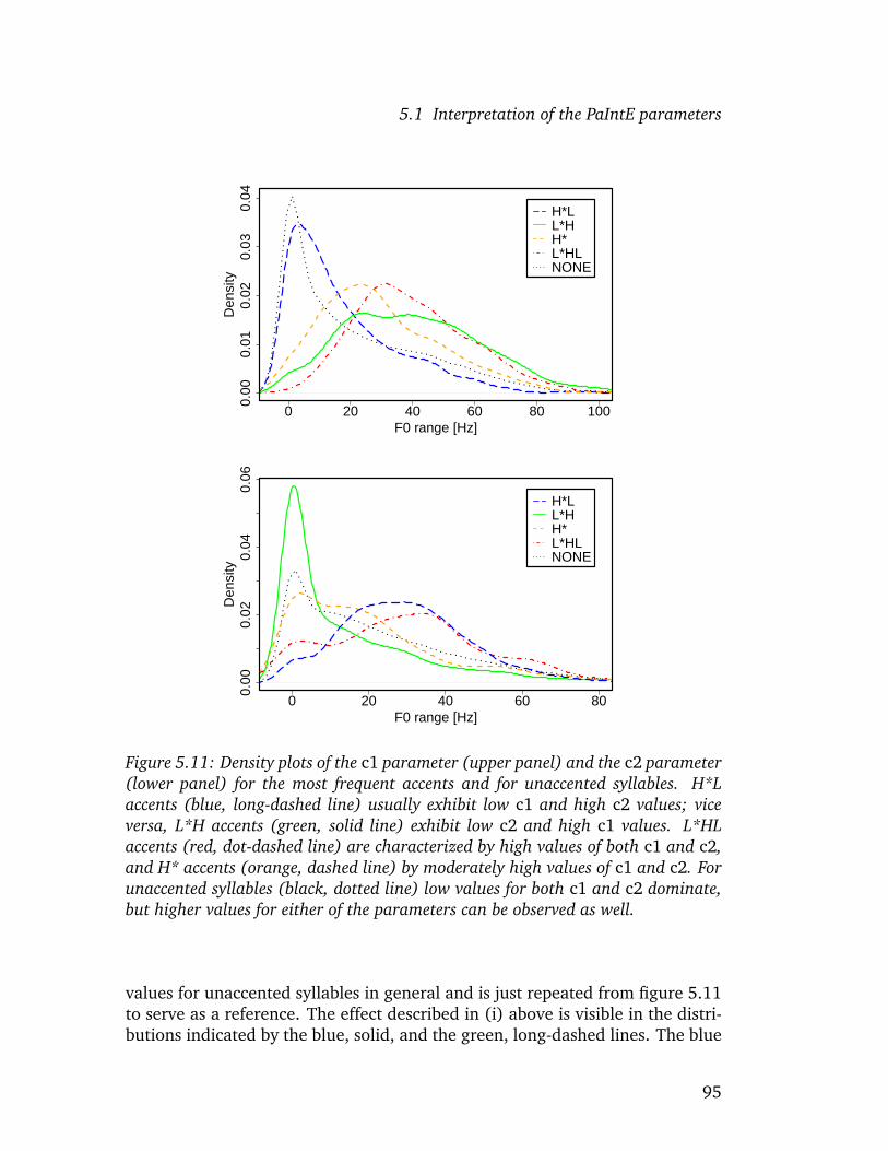
5.1 Interpretation of the PaIntE parameters

0 20 40 60 80 100

0.00

0.01

0.02

0.03

0.04

F0 range [Hz]

Den

sity

H*LL*HH*L*HLNONE

0 20 40 60 80

0.00

0.02

0.04

0.06

F0 range [Hz]

Den

sity

H*LL*HH*L*HLNONE

Figure 5.11: Density plots of the c1 parameter (upper panel) and the c2 parameter(lower panel) for the most frequent accents and for unaccented syllables. H*Laccents (blue, long-dashed line) usually exhibit low c1 and high c2 values; viceversa, L*H accents (green, solid line) exhibit low c2 and high c1 values. L*HLaccents (red, dot-dashed line) are characterized by high values of both c1 and c2,and H* accents (orange, dashed line) by moderately high values of c1 and c2. Forunaccented syllables (black, dotted line) low values for both c1 and c2 dominate,but higher values for either of the parameters can be observed as well.

values for unaccented syllables in general and is just repeated from figure 5.11to serve as a reference. The effect described in (i) above is visible in the distri-butions indicated by the blue, solid, and the green, long-dashed lines. The blue

95

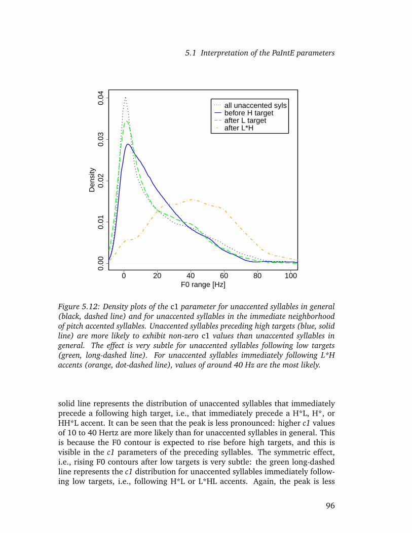
5.1 Interpretation of the PaIntE parameters

0 20 40 60 80 100

0.00

0.01

0.02

0.03

0.04

F0 range [Hz]

Den

sity

all unaccented sylsbefore H targetafter L targetafter L*H

Figure 5.12: Density plots of the c1 parameter for unaccented syllables in general(black, dashed line) and for unaccented syllables in the immediate neighborhoodof pitch accented syllables. Unaccented syllables preceding high targets (blue, solidline) are more likely to exhibit non-zero c1 values than unaccented syllables ingeneral. The effect is very subtle for unaccented syllables following low targets(green, long-dashed line). For unaccented syllables immediately following L*Haccents (orange, dot-dashed line), values of around 40 Hz are the most likely.

solid line represents the distribution of unaccented syllables that immediatelyprecede a following high target, i.e., that immediately precede a H*L, H*, orHH*L accent. It can be seen that the peak is less pronounced: higher c1 valuesof 10 to 40 Hertz are more likely than for unaccented syllables in general. Thisis because the F0 contour is expected to rise before high targets, and this isvisible in the c1 parameters of the preceding syllables. The symmetric effect,i.e., rising F0 contours after low targets is very subtle: the green long-dashedline represents the c1 distribution for unaccented syllables immediately follow-ing low targets, i.e., following H*L or L*HL accents. Again, the peak is less

96

5.1 Interpretation of the PaIntE parameters

0.0

0.2

0.4

0.6

0.8

1.0

Den

sity

−1preceding

L*H

0unaccented

syl

1syl

2

Figure 5.13: Density plot of the b parameter for unaccented syllables with c1>20which occur immediately after an L*H accented syllable. The unaccented syllable,for which the approximation was carried out, is highlighted in gray. The corre-sponding peak is usually detected on the unaccented syllable.

pronounced, i.e., values around 0 are less likely than for unaccented syllablesin general. However, this effect is not very strong and demonstrates that the F0contour does not necessarily start to rise again immediately after low targets.

The distribution of c1 for unaccented syllables immediately following L*Haccents (orange, dot-dashed line) illustrates the effect described in (ii) above:the tonal movement related to the preceding L*H syllable is captured in thePaIntE parametrization of the following unaccented syllable. The distributionshows that the following unaccented syllables usually exhibit c1 parametersof between 20 and 60 Hertz, with few occurrences of values equal to 0. Theeffect is due to the PaIntE approximation being carried out in a three-syllablewindow around the current (in this case unaccented) syllable, and detectedpeaks can be on any of the three syllables. The c1 parameter gives the relativeheight of this peak, no matter on which syllable the peak is realized. So if inthe approximation, a peak is found on a neighboring syllable, the c1 parameterindicates the height of that peak and thus the amplitude of the rise on theneighboring syllable.

I will verify this for the cases with unexpectedly high values of c1, by look-ing at the distribution of unaccented syllables after L*H accents with values of

97

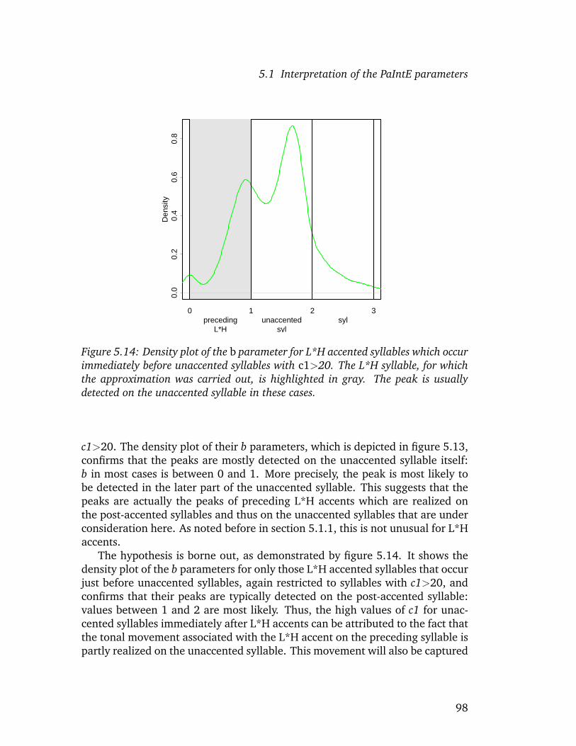
5.1 Interpretation of the PaIntE parameters

0.0

0.2

0.4

0.6

0.8

Den

sity

0preceding

L*H

1unaccented

syl

2syl

3

Figure 5.14: Density plot of the b parameter for L*H accented syllables which occurimmediately before unaccented syllables with c1>20. The L*H syllable, for whichthe approximation was carried out, is highlighted in gray. The peak is usuallydetected on the unaccented syllable in these cases.

c1>20. The density plot of their b parameters, which is depicted in figure 5.13,confirms that the peaks are mostly detected on the unaccented syllable itself:b in most cases is between 0 and 1. More precisely, the peak is most likely tobe detected in the later part of the unaccented syllable. This suggests that thepeaks are actually the peaks of preceding L*H accents which are realized onthe post-accented syllables and thus on the unaccented syllables that are underconsideration here. As noted before in section 5.1.1, this is not unusual for L*Haccents.

The hypothesis is borne out, as demonstrated by figure 5.14. It shows thedensity plot of the b parameters for only those L*H accented syllables that occurjust before unaccented syllables, again restricted to syllables with c1>20, andconfirms that their peaks are typically detected on the post-accented syllable:values between 1 and 2 are most likely. Thus, the high values of c1 for unac-cented syllables immediately after L*H accents can be attributed to the fact thatthe tonal movement associated with the L*H accent on the preceding syllable ispartly realized on the unaccented syllable. This movement will also be captured

98

5.1 Interpretation of the PaIntE parameters

in the PaIntE parameters of the unaccented syllable.10

To summarize the discussion of the c1 and c2 parameters of unaccentedsyllables, it can be said that unaccented syllables tend to have low c1 and c2parameters, indicating that there are usually no pronounced F0 rises or falls onunaccented syllables. Higher values of c1 and c2 can occur because of tonaltargets in the vicinity of the unaccented syllables, which cause the F0 contourto rise or fall, or from the fact that tonal movements associated with the sur-rounding syllables are captured in the PaIntE parametrization of the unaccentedsyllables.

With respect to boundary tones, one would expect high values of c1 for thehigh boundary tones, which should exhibit a rising contour, while low bound-aries should have c1 close to 0. This expectation is borne out as can be seenin figure 5.15. The probability distribution for (L)% (green solid line) shows avery strong preference for values close to or equal to 0, while the three distri-butions for high boundaries (orange dot-dashed line for (H)-, red dashed linefor (H)%, and blue long-dashed line for H%) almost always have c1 values ofmore than 20 Hertz, with the highest values a little more likely to belong tothe inherently high H% boundaries. In light of the fact discussed at the end ofsection 5.1.1 that for (L)% boundaries, the peak is almost always detected onthe final syllable or on one of the syllables preceding it, but almost never onthe next syllable, it is not surprising that c1 values close to 0 predominate for(L)% boundaries: Rises should only be expected from the final syllable with the(L)% boundary to the next phrase, but since the peak is always detected on oneof the earlier syllables, the c1 value always corresponds to the rise toward thatearlier peak. I have suggested above that these earlier peaks are in most casesdue to microprosodic variation, thus their amplitudes are usually low, yieldingonly small values for c1.

For the c2 parameter (figure 5.16), non-zero amplitudes for all boundarytypes are observed. Although there are cases where c2 is close to or equal to 0for all boundary types, as can be seen from the small peaks or at least bumpsat around 0 in the density plots (green solid line for (L)%, orange dot-dashedline for (H)-, red dashed line for (H)%, and blue long-dashed line for H%), themajority of boundaries is realized with fall amplitudes greater than 0. For (L)%boundaries, this is not surprising because they should be realized as falls, butit may be surprising at first in the case of high boundaries. However, I havediscussed above (cf. 5.1.1) that for high boundaries, falling pitch movements

10It may be noted that this distribution of the b parameter looks different from the one forL*H depicted in figure 5.5. There, the peak was almost equally likely on the accented and onthe post-accented syllable. The distribution depicted here is different because only L*H accentsbefore unaccented syllables with values of c1>20 are taken into account. In cases where thepeak is realized on the accented syllable, if some small peak is detected on the unaccentedsyllable, this peak will be approximated rather than the peak of the preceding accent, givingrise to lower c1 values, and thus such cases are not included in the distribution depicted here.

99

5.1 Interpretation of the PaIntE parameters

0 20 40 60 80 100

0.00

0.05

0.10

0.15

0.20

F0 range [Hz]

Den

sity

H%(H)%(L)%(H)−NONE

Figure 5.15: Density plots of the c1 parameter for the most frequent boundarytones and for non-final syllables. (L)% boundaries (green, solid line) and unac-cented syllables (black, dotted line) usually have low c1 parameters, while highboundaries exhibit higher values of c1.

are detected because the reset of F0 for the next phrase causes a drop in F0 atthe boundary to the next syllable. The amplitude of the drop is documented inthe c2 parameter for the high boundaries.

Again, I will conclude this section by confirming that the observed differ-ences are significant. Table 5.3 lists the p-values obtained in pairwise Wilcoxonrank sum tests of the c1 distributions for accents and boundaries. The distri-butions for unaccented syllables (NONE) vs. H*L accents are not significantlydifferent, neither are those for L*H vs. L*HL; all other distributions are signif-icantly different at a confidence level of 0.999. The p-values resulting fromcomparing the c2 distributions are indicated in table 5.4. Here, the distributionsfor unaccented syllables (NONE) vs. H* accents are not significantly different,neither are those for H*L vs. L*HL; as for boundaries, there is no significant dif-ference between H% and (H)%, between H% and (H)-, and between (H)% and(L)%; the other distributions are significantly different at a confidence level of0.999.

100

5.1 Interpretation of the PaIntE parameters

0 20 40 60 80 100

0.00

0.01

0.02

0.03

F0 range [Hz]

Den

sity

H%(H)%(L)%(H)−NONE

Figure 5.16: Density plots of the c2 for the most frequent boundary tones andfor non-final syllables. Unaccented syllables (black, dotted line) tend to have lowvalues of c2, but higher values can also occur. For boundaries, values of c2 ofaround 0 do occur, but in the majority of cases, higher values are detected.

Concluding this subsection, it can be stated that the PaIntE parameter dis-tributions of GToBI(S) events reflect the expected tonal properties. I have notdiscussed parameters a1 and a2, which determine the steepness of the relatedrise or fall, because GToBI(S) makes no prediction of what their probabilitydistributions might look like. However, this does not necessarily speak againsttheir perceptual relevance. I will leave open this question for now. However, Ipropose to view them as potentially relevant in perception. In the following, Iwill for the sake of simplicity speak of “the” PaIntE parameters as perceptuallyrelevant, but one should keep in mind that the perceptual relevance of a1 anda2 is less well motivated than that of the remaining parameters.

101

5.2 Target regions for intonation events

NONE H*L H* L*H L*HLNONE – 0.10361 0.00000 0.00000 0.00000H*L 0.10361 – 0.00000 0.00000 0.00000H* 0.00000 0.00000 – 0.00000 0.00000L*H 0.00000 0.00000 0.00000 – 0.61154L*HL 0.00000 0.00000 0.00000 0.61154 –

NONE H % (H)% (H)- (L)%NONE – 0.00000 0.00000 0.00000 0.00000H% 0.00000 – 0.00000 0.00000 0.00000(H)% 0.00000 0.00000 – 0.00002 0.00000(H)- 0.00000 0.00000 0.00002 – 0.00000(L)% 0.00000 0.00000 0.00000 0.00000 –

Table 5.3: p-values obtained by pairwise Wilcoxon rank sum tests comparing dis-tributions of c1 for the most frequent accent types (upper panel) and boundarytypes (lower panel). The distributions for unaccented syllables (NONE) vs. H*Laccents are not significantly different, neither are those for L*H vs. L*HL; all otherdistributions are significantly different at a confidence level of 0.999. Values of0.00000 indicate that p�0.000005.

5.2 Target regions for intonation events

At the very beginning of this chapter, I have presented three questions, two ofwhich I claim to answer here: (i) what are the tonal dimensions of perceptualspace, (ii) which are the relevant prosodic events, and (iii) which are the targetregions corresponding to these events. I have already stated above that in thepresent thesis, I will assume that the prosodic events as defined by GToBI(S)(Mayer 1995) are the relevant prosodic events.

As for question (i), I have argued in chapter 3 that the PaIntE parametersare linguistically motivated in that they are intended to model aspects of therealization of intonation events that are known to be meaningful. In this chap-ter, I have explained the relation between the PaIntE parameters and the pitchaccents and boundary tones of the GToBI(S) labeling system. I have shownempirically that the PaIntE parameters capture the tonal properties attributedto the different intonation events posited by GToBI(S), and that rather fine-grained effects of prosodic and segmental context on the tonal implementationof these events are visible in the probability distributions of their PaIntE param-eters.

Since these events are defined as tonally distinct units, it goes without say-ing that they will differ with respect to their tonal properties. I have explained

102

5.2 Target regions for intonation events

NONE H*L H* L*H L*HLNONE – 0.00000 0.07034 0.00000 0.00000H*L 0.00000 – 0.00000 0.00000 0.81739H* 0.07034 0.00000 – 0.00000 0.00000L*H 0.00000 0.00000 0.00000 – 0.00000L*HL 0.00000 0.81739 0.00000 0.00000 –NONE – 0.00000 0.00000 0.00000 0.00000H% 0.00000 – 0.06971 0.01203 0.00000(H)% 0.00000 0.06971 – 0.00002 0.00761(H)- 0.00000 0.01203 0.00002 – 0.00000(L)% 0.00000 0.00000 0.00761 0.00000 –

Table 5.4: p-values obtained by pairwise Wilcoxon rank sum tests comparing dis-tributions of c2 for the most frequent accent types (upper panel) and boundarytypes (lower panel). In the upper panel, the distributions for unaccented syllables(NONE) vs. H* accents are not significantly different, neither are those for H*Lvs. L*HL; in the lower panel, there is no significant difference between H% and(H)%, between H% and (H)-, and between (H)% and (L)%; all other distribu-tions are significantly different at a confidence level of 0.999. Values of 0.00000indicate that p�0.000005.

above how the PaIntE parameters serve to distinguish between the different in-tonation events: The probability distributions of the PaIntE parameters differfor different events. These differences were not always present in every pa-rameter; rather, some parameters are similar for some intonation events, butuseful in distinguishing between other intonation events, and others vice versa.For example, the distributions for the b parameter are quite different for H*Laccents and L*H accents, but more similar for H* an L*HL accents (cf. figure5.4), while for H* and L*HL accents the distributions for the c2 parameter aredifferent (cf. figure 5.11).

Building on these two aspects—that the PaIntE parameters model propertiesof the realization of intonation events that are meaningful and that they serveto distinguish different categories—I propose to answer question (i) by consid-ering the PaIntE parameters as the relevant tonal dimensions in the perceptionand production of intonation events.

Regarding question (iii), which are the target regions corresponding to theprosodic events, in section 2.3.5 I have presented an exemplar-theoretic inter-pretation of Guenther and Perkell’s speech production model (Guenther et al.1998; Perkell et al. 2000, 2001) for the temporal domain. I have suggestedthat z-score distributions implicitly define target regions in the production oftemporal properties of prosodic events. Reasoning the same way for the tonal

103

5.2 Target regions for intonation events

domain, I propose to regard the distributions of PaIntE parameters as targetregions in the production of tonal properties of prosodic events. Thus, the ab-stract perceptual target regions posited by Guenther and Perkell’s model forthe segmental domain are implicitly defined by the distributions of PaIntE pa-rameters of the exemplars stored in the memory of the speaker. This view ismotivated by the fact that if phonetic details of the exemplars are stored inmemory, speakers have access to the F0 contours of the stored exemplars, andtheir shapes in terms of peak alignment, peak height, rise and falls amplitudes,etc., as coded in the PaIntE parameters, and are likely to use them as a referencein production.

Moreover, I have presented experimental results confirming that realiza-tions of syllables in different prosodic contexts show different distributions ofPaIntE parameters, i.e., they are expected to be useful in distinguishing prosodicevents. As with the z-score distributions examined in section 4.3, there is a lotof overlap between the distributions. However, I have only examined one pa-rameter at a time; taking all parameters into account at once may be enoughto make the regions sufficiently distinct from each other. This question will beaddressed in the following chapter.

104

Chapter 6

Modeling categorization

I have shown in chapters 4 and 5 that the distributions of z-scores of segmentdurations in the temporal domain and of the PaIntE parameters in the tonaldomain are significantly different for different prosodic events. With regard toperception, the question that immediately arises is whether these regions aresufficiently distinct to categorize new exemplars. From an exemplar-theoreticpoint of view, new instances are categorized based on their perceptual similarityto exemplars stored in memory (cf. section 2.3.3): they are assigned the cate-gory of the most similar exemplars. I will investigate in this chapter whetherthe perceptual dimensions introduced in the preceding chapters are suitableand sufficient for categorizing new instances.

In spite of the fact that most prosodic events exhibit significantly differentduration z-score and PaIntE parameter distributions, there was a considerableamount of overlap in all distributions. However, I have only examined the per-ceptual dimensions one at a time. Because of the overlap in the distributions,few exemplars could have been categorized correctly based on one dimensiononly. The question that I am trying to answer in this present chapter is whethercategorization is possible when all relevant dimensions contribute to catego-rization.

From a theoretical perspective, listeners are able to categorize new ex-emplars in speech perception. Thus, modeling a listener’s memory by alarge prosodically annotated speech corpus, it should be possible to catego-rize prosodic events if all perceptually relevant dimensions are known, i.e., itshould be possible to predict prosodic labels for new exemplars based on thevalues that exemplars from the corpus exhibit for these dimensions. In the bestcase, one could even hope to detect prosodic categories by identifying accumu-lations of exemplars with similar perceptual properties, and then establishingwhich accumulations correspond to which category.

I will examine both approaches in this chapter. I will discuss clustering ex-periments as a way to detect prosodic categories in section 6.2. I will thenmodel categorization of prosodic events using machine learning methods to

105

6.1 Representing the data

predict prosodic labels in section 6.3. But before turning to the actual experi-ments, I will describe the data used in both approaches in section 6.1.

6.1 Representing the data

In machine learning, whether the goal be clustering or classifying data, the firststep is to represent the data as a set of instances of observations. In the experi-ments presented in this chapter, the data consist of instances of realizations ofsyllables. Each instance is described by some observed properties. These prop-erties are called attributes, and thus each instance is characterized by the valuesthat it exhibits for the attributes. For coherence with the preceding chapters,instances can be thought of as exemplars, and the attributes can be interpretedas their perceptual properties; however, not all attributes I will be using herehave been confirmed as perceptually relevant.

In the following sections, I will first discuss the attributes used for the ex-periments described in this chapter; then, I will provide more details on thedatabases from which the data were extracted in section 6.1.2. Finally, a noteof caution is in order (section 6.1.3) because the data are inevitably noisy.

6.1.1 Attributes

Most attributes used here are related to the duration z-scores and PaIntE pa-rameters discussed in the preceding chapters. However, some more attributesthat were thought to be useful in distinguishing accent types and boundarieswere included, even though I have not examined in detail whether they canbe claimed to be perceptually relevant or not. All attributes are discussed andillustrated using an example sentence from the database in the following. Iwill also explain for each attribute why it has been included, particularly forthe attributes that are not directly related to the duration z-scores or PaIntEparameters.

Tables 6.1 to 6.5 list attributes and observed values of the first thirteen in-stances of syllables of the SWMS corpus, corresponding to the phrase “Das Zen-trum blieb zumeist Cardoso vorbehalten” (The center was mostly left to Cardoso);each line represents an instance, and each column represents an attribute; theobserved values are indicated in the table cells. For the experiments, all in-stances and attributes are collected in one huge table; this table is broken downhere into several partial tables in order to have more space for discussion of theparticular attributes in between tables.

Table 6.1 shows the first eight attributes. The first two specify whichGToBI(S) accent (if any) and which GToBI(S) boundary tone (if any) have been

106

6.1 Representing the data

accent tone a1’ a2’ b c1’ c2’ d’1 NONE NONE -0.443 -0.957 2.045 2.389 -0.976 2.6372 L*HL NONE -0.306 0.624 0.876 2.178 2.695 2.4713 NONE (L)- 0.115 0.239 -0.206 1.389 2.987 2.5494 NONE NONE -0.976 -0.849 0 -0.953 -0.976 -1.3095 NONE NONE -0.57 0.007 0.833 -0.512 -0.646 -1.0426 NONE NONE 0.402 0.001 1.404 -0.61 -0.751 -0.917 NONE NONE 0.126 -0.957 1.732 -0.438 -0.976 -0.4988 H*L NONE -0.284 -0.441 0.997 -0.405 1.124 -0.449 NONE NONE -0.692 0.473 0.44 -0.105 0.101 -0.506

10 NONE NONE 1.715 -0.184 0.475 -0.354 -0.55 -1.04211 NONE NONE 1.495 -0.392 -0.526 -0.353 -0.449 -1.07112 NONE NONE 2.638 -0.957 1.313 -0.687 -0.976 -1.44613 NONE (L) 1.833 0.237 0.344 -0.641 -0.195 -1.415

Table 6.1: Prosodic labels (first two columns, used for evaluation purposes) andfirst six attributes (remaining columns) with corresponding values for the firstthirteen instances of the SWMS data. The six attributes are the PaIntE parametersdetermined for each instance. Values of parameters marked by ’ have been z-scored.

realized on that particular syllable.1 The values for these two attributes havebeen determined by manual prosodic labeling. They are not intended to beused in the clustering or classification experiments themselves, but are pro-vided for evaluation purposes. In the clustering experiments, one hopes to findcorrelations between these manual labels and the observed clusters. In the clas-sification experiments, they are the attributes whose values are to be predictedbased on the values of all other attributes.

The accent attribute corresponds to the GToBI(S) accent label of the sylla-ble, with downstepped accents mapped to their counterparts without downstep.Thus, the attribute can assume the following values: NONE for unaccented syl-lables, or any of the accents of the GToBI(S) annotation system discussed insection 3.1: L*H, H*L, L*, H*, ..H, ..L, L*HL, or HH*L. Please note that tech-nically, ..H and ..L are not accents but trail tones related to an earlier accent.In contrast to the “real” accents, they may also occur on unstressed syllables.For the tone attribute, I have again mapped the underspecified boundary tones% and - of the GToBI(S) system to fully specified tones by integrating the pre-ceding trail tone into the boundary tone labels (cf. chapter 5): to distinguishthem from boundary tones that had been fully specified already, the precedingtrail tones are specified in brackets. Thus, values of (H)%, for instance, occur

1GToBI(S) is discussed in more detail in section 3.1.

107

6.1 Representing the data

for syllables with an originally unspecified % boundary tone after a precedingH trail tone (which must have come from a preceding L*H accent), while H%occurs if the boundary tone had been fully specified in the manual prosodic an-notation already. The full set of possible values for the tone attribute is NONEfor non-final syllables, or (H)-, (L)-, (H)%, H%, (L)%, or L% for phrase-finalsyllables.

The remaining attributes in table 6.1 are attributes whose values are actuallyused for clustering or learning. They correspond to the six PaIntE parameters(cf. chapter 3). As I have substantiated in some detail in chapter 5, the PaIntEparameters are expected to be relevant in the perception of prosodic events.Since the experiments aim at modeling categorization, it is desirable to buildmodels that are applicable to data of different speakers. However, at least threeof the six PaIntE parameters are expected to be speaker-specific: d correspondsto the absolute height of the F0 peak in Hertz, which will be different betweenspeakers, particularly between male and female speakers. c1 and c2 specifythe amplitudes of the rising or falling F0 movement. It is often claimed thatfemale speakers have a greater F0 range, therefore the amplitudes of the F0movement in accented syllables are expected to be greater for female than formale speakers. Thus, c1 and c2 should be speaker-specific or at least gender-specific. To eliminate the speaker-specific aspects, d, c1, and c2 were z-scored.Parameters a1 and a2 correspond to the amplitude-normalized steepness ofthe rising and falling movements, respectively. As the amplitudes (c1 and c2)are likely to be speaker-specific, the amplitude normalization introduces somespeaker-specificity, and thus, a1 and a2 have been z-scored as well.2 The bparameter was left unchanged because there was no equally compelling reasonto expect speaker-specific effects: parameter b corresponds to the alignment ofthe F0 peak with the syllable structure and there is no evidence that speakersmight differ in that respect.3 To the contrary, it is not advisable to z-score theb parameter since its values are normalized with respect to syllable structure,with integer values corresponding to syllable boundaries. Thus, z-scoring the bparameter would obscure the peak’s exact position in the syllable.

In any case, z-scoring of five of the six PaIntE parameters seems to have beenunproblematic, as I have applied most of the classification algorithms discussedin section 6.3 to both the absolute and z-scored values of these parameters, andthere was no indication whatsoever that performance might have been lowerin the z-scored case. The z-scored parameters are marked by the ’ diacritic inthe remainder of this chapter.

2I do not claim that listeners z-score or otherwise normalize the tonal parameters in per-ception; z-scoring here is just a technicality that is necessary to be able to apply the models andclassifiers obtained on data of just one speaker to data of other speakers later.

3I do not want to deny that dialects might differ in the alignment of peaks, but dialectalvariation is beyond the scope of this thesis. Here, I model categorization of speakers of thesame dialect, viz. Standard German (“Hochdeutsch”).

108

6.1 Representing the data

maxc c1’-c2’prev syl next syl

pc1’ pc2’ pd’ nc1’ nc2’ nd’1 2.389 -3.364 -0.953 -0.976 -5.612 2.178 2.695 2.4712 2.695 0.518 2.389 -0.976 2.637 1.389 2.987 2.5493 2.987 1.598 2.178 2.695 2.471 -0.953 -0.976 -1.3094 -0.953 -0.022 1.389 2.987 2.549 -0.512 -0.646 -1.0425 -0.512 -0.133 -0.953 -0.976 -1.309 -0.61 -0.751 -0.916 -0.61 -0.141 -0.512 -0.646 -1.042 -0.438 -0.976 -0.4987 -0.438 -0.538 -0.61 -0.751 -0.91 -0.405 1.124 -0.448 1.124 1.529 -0.438 -0.976 -0.498 -0.105 0.101 -0.5069 0.101 0.206 -0.405 1.124 -0.44 -0.354 -0.55 -1.04210 -0.354 -0.196 -0.105 0.101 -0.506 -0.353 -0.449 -1.07111 -0.353 -0.096 -0.354 -0.55 -1.042 -0.687 -0.976 -1.44612 -0.687 -0.289 -0.353 -0.449 -1.071 -0.641 -0.195 -1.41513 -0.195 0.446 -0.687 -0.976 -1.446 0.809 -0.976 0.614

Table 6.2: Attributes 7 to 14 and corresponding values for the first ten instances ofthe SWMS data. The first two attributes indicate the maximum amplitude on thecurrent syllable as determined by max(c1’,c2’) and the difference between c1’ andc2’. The remaining attributes in this table correspond to the PaIntE parametersc1, c2 and d of the preceding (attributes pc1’, pc2’, pd’) and following syllables(attributes nc1’, nc2’, nd’).

Table 6.2 lists further attributes used in the following sections. The firstone, maxc, is the maximum of c1’ and c2’. This attribute was included tocapture the maximum amplitude of the F0 movement on the syllable in oneparameter, irrespective of whether it is related to a rise or to a fall, and might behelpful in distinguishing unaccented syllables from accented ones, for instance.The second, c1’-c2’, codes the relative difference in F0 before and after the F0movement by subtracting the amplitude of the falling movement, c2’, from theamplitude of the rising movement, c1’. Thus, F0 movements for which c2’ wasgreater than c1’, which can be interpreted as overall falling, are characterizedby negative values, whereas F0 movements with greater c1’ than c2’, which canbe described as overall rising, exhibit positive values for c1’-c2’.

The other attributes in table 6.2 are z-scored PaIntE parameters of the pre-ceding (attributes pc1’, pc2’, pd’) and following syllables (attributes nc1’, nc2’,nd’). They are of interest because comparison of these parameters for adjacentsyllables can indicate local changes in the slope of the F0 contour. Assume, forinstance, that there is a longer rising stretch of F0 spanning several syllables.All syllables within that span should have moderately high, positive, and, mostimportant, similar, values of c1 (and c2 parameters around 0). Here, the sim-

109

6.1 Representing the data

syl before preceding syl syl after next sylppc1’ ppc2’ ppd’ nnc1’ nnc2’ nnd’

1 -0.953 -0.976 -5.612 1.389 2.987 2.5492 -0.953 -0.976 -5.612 -0.953 -0.976 -1.3093 2.389 -0.976 2.637 -0.512 -0.646 -1.0424 2.178 2.695 2.471 -0.61 -0.751 -0.915 1.389 2.987 2.549 -0.438 -0.976 -0.4986 -0.953 -0.976 -1.309 -0.405 1.124 -0.447 -0.512 -0.646 -1.042 -0.105 0.101 -0.5068 -0.61 -0.751 -0.91 -0.354 -0.55 -1.0429 -0.438 -0.976 -0.498 -0.353 -0.449 -1.071

10 -0.405 1.124 -0.44 -0.687 -0.976 -1.44611 -0.105 0.101 -0.506 -0.641 -0.195 -1.41512 -0.354 -0.55 -1.042 0.809 -0.976 0.61413 -0.353 -0.449 -1.071 0.457 -0.976 0.266

Table 6.3: Attributes 15 to 20 and corresponding values for the first thirteen in-stances of the SWMS data. The attributes indicate PaIntE parameters c1, c2 andd of the syllables before the preceding (attributes ppc1’, ppc2’, ppd’) and after thefollowing syllable (attributes nnc1’, nnc2’, nnd’).

ilarity of the c1 values is an indicator that this is not a local F0 rise caused byan accent but a more global F0 movement, possibly caused by the interpolationbetween a preceding low and a following high target. For the same reason,the parameters of the syllable before the preceding syllable (attributes ppc1’,ppc2’, ppd’) and the syllable after the next syllable (attributes nnc1’, nnc2’,nnd’) are also included. These are listed in table 6.3.4

The attributes cited so far are all related to the PaIntE parametrization. Inshort, all PaIntE parameters of the current syllable are used. Also, the maximumof c1’ and c2’ and the difference between c1’ and c2’ are provided. And finally,

4It should be noted that file boundaries are ignored when calculating the PaIntE parametersof the context syllables in order to avoid artifacts caused by the structure of the database.Usually, after running a PaIntE approximation for an utterance which corresponds to one speechfile, for the first syllables, the PaIntE parameters of the left context syllables are not accessible,and for the last syllables, the PaIntE parameters of the right context syllables are missing.Thus, file boundaries, which virtually always coincide with phrase boundaries, might be easilydetectible from the missing parameters. This could artificially increase the prediction accuracyof phrase boundaries for corpora like the SWMS corpus, which consist of rather short utterancesin many separate files. Instead, the context syllables are taken from preceding or following filesif necessary. This way, the only cases where the PaIntE parameters of the context are notaccessible are the very first and the very last syllables of the corpus. In these few cases, theabsolute parameters have been set to 0, resulting in negative z-scored values of -0.953, -0.976,and -5.612 for c1’, c2’, and d’, respectively.

110

6.1 Representing the data

in addition to the PaIntE parameters of the current syllable, c1’, c2’ and d’ of thetwo preceding and the two following syllables are used; thus, these parametersare provided for a five-syllable window around the syllable in question.

Turning to temporal aspects, I have motivated in chapter 4 that phoneme-specific z-scores of segment durations are relevant in the perception of prosodicevents. I have shown in section 4.3 that lengthening effects caused by accentsare most prominent for onset segments and syllable nuclei (figure 4.8), whileeffects caused by phrase boundaries are most prominent for the last (phrase-final) segment (figure 4.7). Therefore, both the z-scores for nuclei5 and thez-scores for final segments are provided. The former should be helpful in distin-guishing accented syllables from unaccented syllables, the latter in recognizingphrase boundaries. Again, in order to facilitate comparison of values for thecurrent syllable with those for context syllables, these attributes are providedfor a three-syllable window around the current syllable. Comparing durationz-scores of the current syllable to that of context syllables should help to sepa-rate effects of prosodic events from effects of local speech rate: If lengthening iscaused by a low speech rate, the z-scores of the context syllables should be sim-ilar, while, if lengthening is caused by prosodic events, context syllables shouldnot be affected. Thus, six attributes are relevant: phoneme-specific durationz-scores of nuclei of the current (attribute nucleus), preceding (attribute pnu-cleus), and next syllables (attribute nnucleus) and phoneme-specific durationz-scores of final segments of the current (attribute finalseg), preceding (at-tribute pfinalseg), and next syllables (attribute nfinalseg). Again, the valuesof these attributes for the first thirteen instances are indicated in table 6.4.6

All attributes discussed so far are numeric. The remaining attributes arenominal attributes that are either derived from the annotation of the databaseor even from the underlying text. They are listed in table 6.5. The first threecan be classified as phonological and are derived directly from the segment,syllable, and word label files. The stress attribute indicates whether a syllableis stressed or not, possible values are 1 (for stressed) and 0 (for unstressed).For clustering and classification of accents, it is clearly advantageous to knowwhich syllables are stressed, since the accents can only occur on stressed sylla-bles. I would hypothesize that even human listeners in the perception of accentsare aware of the location of stressed syllables and use that information whencategorizing accents, although I cannot confirm this hypothesis by formal ex-

5Since the lengthening effect is intended to be captured in just one attribute, it is straight-forward to take the nucleus z-score instead of z-scores of possibly several segments, whichwould have to be condensed into one value.

6File boundaries are ignored when accessing the duration z-scores of the context syllables,for the same reason as in the case of the PaIntE parameters of the context syllables (cf. footnote4). Again, the only cases where the z-score parameters of the context are not accessible are thevery first and the very last syllables of the corpus. In these few cases, the absolute parametershave been set to 0.

111

6.1 Representing the data

nucleus duration final segment durationnucleus pnucleus nnucleus finalseg pfinalseg nfinalseg

1 -0.876 0 0.32 -0.009 0 0.322 -0.183 -0.009 1.237 0.32 -0.009 1.2373 0.427 0.32 -1.953 1.237 0.32 -1.9534 -0.601 1.237 -0.958 -1.953 1.237 -0.9585 -0.958 -1.953 -1.248 -0.958 -1.953 -1.2486 -0.399 -0.958 -0.679 -1.248 -0.958 -0.6797 -0.896 -1.248 0.728 -0.679 -1.248 0.7288 0.728 -0.679 -0.057 0.728 -0.679 -0.0579 -0.057 0.728 -0.976 -0.057 0.728 -0.976

10 -0.509 -0.057 1.283 -0.976 -0.057 1.28311 1.283 -0.976 0.48 1.283 -0.976 0.4812 -0.165 1.283 3.783 0.48 1.283 3.78313 -0.862 0.48 -1.139 3.783 0.48 -1.139

Table 6.4: Attributes 21 to 26 and corresponding values for the first thirteen in-stances of the SWMS data. The attributes indicate phoneme-specific duration z-scores of nuclei of the current (nucleus), preceding (pnucleus), and next syllables(nnucleus), and phoneme-specific duration z-scores of final segments of the cur-rent (finalseg), preceding (pfinalseg), and next syllables (nfinalseg).

periments currently. However, when trying to prosodically label speech basedon the larynx signal only, where only the F0 information is present, I foundthat in some cases where there was a peak in the F0 contour derived from thelarynx signal, I could not tell whether the peak was the high target of a risingL*H accent on a preceding syllable or whether it was a high target correspond-ing to an H* or H*L accent at the current location. The location of the wordstress could have disambiguated the contour in these cases—if the high targetco-occurs with a stressed syllable, it is likely to be the high target of an H* orH*L accent, and unlikely to be the high trail tone of an L*H, because that wouldrather be expected on the following syllable.

The wordfin attribute indicates whether the syllable is word-final or not; itcan take values of 0 (word-internal) or 1 (word-final). Similar to the relevanceof the stress attribute in clustering or classifying accents, the wordfin attributeis evidently helpful in recognizing boundaries since word-internal syllables atleast in unmarked speech are never phrase-final and thus should never exhibitboundary tones. Again, I would hypothesize that human listeners make use ofthis information as well. Phrase boundaries, particularly intermediate phraseboundaries, are very hard to recognize when labeling speech based on the lar-

112

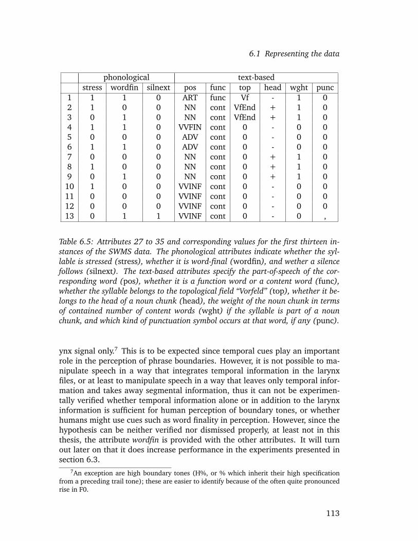
6.1 Representing the data

phonological text-basedstress wordfin silnext pos func top head wght punc

1 1 1 0 ART func Vf - 1 02 1 0 0 NN cont VfEnd + 1 03 0 1 0 NN cont VfEnd + 1 04 1 1 0 VVFIN cont 0 - 0 05 0 0 0 ADV cont 0 - 0 06 1 1 0 ADV cont 0 - 0 07 0 0 0 NN cont 0 + 1 08 1 0 0 NN cont 0 + 1 09 0 1 0 NN cont 0 + 1 0

10 1 0 0 VVINF cont 0 - 0 011 0 0 0 VVINF cont 0 - 0 012 0 0 0 VVINF cont 0 - 0 013 0 1 1 VVINF cont 0 - 0 ,

Table 6.5: Attributes 27 to 35 and corresponding values for the first thirteen in-stances of the SWMS data. The phonological attributes indicate whether the syl-lable is stressed (stress), whether it is word-final (wordfin), and wether a silencefollows (silnext). The text-based attributes specify the part-of-speech of the cor-responding word (pos), whether it is a function word or a content word (func),whether the syllable belongs to the topological field “Vorfeld” (top), whether it be-longs to the head of a noun chunk (head), the weight of the noun chunk in termsof contained number of content words (wght) if the syllable is part of a nounchunk, and which kind of punctuation symbol occurs at that word, if any (punc).

ynx signal only.7 This is to be expected since temporal cues play an importantrole in the perception of phrase boundaries. However, it is not possible to ma-nipulate speech in a way that integrates temporal information in the larynxfiles, or at least to manipulate speech in a way that leaves only temporal infor-mation and takes away segmental information, thus it can not be experimen-tally verified whether temporal information alone or in addition to the larynxinformation is sufficient for human perception of boundary tones, or whetherhumans might use cues such as word finality in perception. However, since thehypothesis can be neither verified nor dismissed properly, at least not in thisthesis, the attribute wordfin is provided with the other attributes. It will turnout later on that it does increase performance in the experiments presented insection 6.3.

7An exception are high boundary tones (H%, or % which inherit their high specificationfrom a preceding trail tone); these are easier to identify because of the often quite pronouncedrise in F0.

113

6.1 Representing the data

The last of the “phonological” attributes is silnext. It specifies whether asilence follows (in which case its value is 1, otherwise 0). It is evident that thesilnext attribute should be a good indicator of phrase boundaries since silences,i.e. pauses, are very frequent at phrase boundaries.

The remaining attributes are “text-based” attributes which are derived fromorthographic information and punctuation marks. These attributes are a sub-set of the attributes used by the prosody prediction module of the IMS Festivaltext-to-speech synthesis system (IMS Festival 2010). Thus, they are known tobe predictive of prosodic structure, and they were included mainly to see if theirpresence would increase performance—given that they contribute in text-basedprediction of prosodic events, they might be helpful in the (phonetically based)classification experiments as well. The attribute pos specifies the part-of-speech(POS) tag of the word that the syllable is related to. POS tags were obtainedby the German Tree Tagger (Schmid 1994, 1995), which uses the STTS tag set(Schiller et al. 1995). The STTS tag set comprises 12 main classes of POS tags(adjectives, adverbs, adpositions, determiners, cardinals, interjection, conjunc-tions, nouns, pronouns, particles, verbs, and miscellaneous), which are furthersubdivided into altogether 54 different types of POS tags. For instance, verbsare subdivided into full verbs, modal verbs, and auxiliary verbs, and for eachof these subclasses, STTS distinguishes between finite verbs, imperative forms,infinitives, and participles, yielding 12 different POS tags pertaining to verbforms. I have also included the attribute func, which maps the POS tags to justtwo classes for function and content word (values: func, cont) in the followingway: adpositions, determiners, conjunctions, pronouns, particles, and auxiliaryverb forms are function words, everything else is classified as content word.

The attribute top is also derived from the POS tags. It specifies whetherthe syllable belongs to the so-called Vorfeld, if it ends the Vorfeld, or if it is notpart of the Vorfeld at all. Vorfeld is a term which was introduced by topologicalmodels of German syntax (e.g., Hohle (1986), or see Grewendorf et al. (1989)for a description of topological models in general). These models state that sen-tences are divided into topological fields: Vorfeld, left bracket, Mittelfeld, rightbracket, and Nachfeld (note that the right bracket is called “Verbalkomplex” byHohle (1986)). The Vorfeld can accommodate exactly one constituent, whichis often the subject. The left bracket is reserved for either the finite verb (inmain clauses) or for conjunctions (in subordinate clauses). However, in the lat-ter case the Vorfeld must remain empty. Thus, the occurrence of the finite verbis a good indicator of the boundary of a preceding constituent of possibly highcomplexity, which is why our TTS prosody prediction module assigns prosodicphrase boundaries at the end of the Vorfeld if the length of the Vorfeld exceedsa certain threshold. The end of the Vorfeld is located by the occurrence of aPOS tag indicating the finite verb. Possible values of the top attribute are VF(for words contained in the Vorfeld), VFEnd (for the final word in the Vorfeld),and 0 (else).

114

6.1 Representing the data

Another concept that is used for predicting prosodic events in our TTS sys-tem is the noun chunk. According to Abney (1995), chunks are those fragmentsof a parse tree that remain when detaching all elements whose attachment tothe tree is not unambiguous, and chunk boundaries correspond to prosodicboundaries. Interpreting Abney in a simplistic way, noun chunks thus can onlyconsist of possibly a determiner, followed by zero to several adverbs and ad-jectives, and one to several nouns. Modifications by prepositional phrases, forinstance, would give rise to their own, separate noun chunk, because the at-tachment of prepositional phrases would be ambiguous. Thus, using the POStags obtained from the Tree Tagger, noun chunks can be approximately iden-tified by their typical patterns of sequences of POS tags. Noun chunks are notonly predictive of prosodic boundaries; they also often carry pitch accents, usu-ally on the final noun, because of the right-branching structure of German nounphrases. Thus, the final noun in a noun chunk not only signals a potential sitefor a prosodic boundary, it is also a candidate site for a pitch accent. In theIMS German Festival TTS system, final nouns in noun chunks are therefore re-ferred to as head of the noun chunk. The classification of a word as being thehead of a noun chunk, based on the identification of noun chunk boundariesby patterns of POS tags from the Tree Tagger, is captured in the head attribute(values +, -). Since the length of noun chunks also seems to be relevant forthe assignment of prosodic boundaries or accents (very short noun chunks areless likely to be realized with prosodic boundaries, for instance), we also deter-mine their weight in terms of number of content words in the noun chunk. Thisweight is indicated by the wght attribute; it can take positive integer numbersfor syllables in noun chunks, or 0 for syllables which do not belong to nounchunks.

The last attribute, punc, specifies whether there was a punctuation sym-bol after the syllable in the text underlying the utterance (i.e., in the text thespeaker was prompted with). Possible values are 0 (for no punctuation) or anyof the following symbols: ,;:?!.)”

6.1.2 Databases for training and testing

The data (i.e., the attributes for each syllable instance) were extracted from twodatabases, viz. the SWMS database (2 hrs., male) and the SWRK database (3hrs., female), which had been recorded in the course of the SmartWeb project(Wahlster 2004). The speakers are professional speakers of Standard German.For both databases, the utterances represent typical utterances of 5 differentgenres. They were read off a screen at recording time. Afterwards, the utter-ances were annotated on the segment, syllable, and word level, and prosodi-cally labeled according to GToBI(S) (Mayer 1995). Prosodic labeling for eachutterance was carried out by one of three human labelers, all supervised and

115

6.1 Representing the data

instructed by myself, without having the present experiments in mind. TheSWMS database amounts to 72,000 segments, 28,000 syllables, and 14,000words. The SWRK data contain 88,000 segments, 34,000 syllables, and 17,000words.

The databases were originally used for unit selection speech synthesis inthe SmartWeb project (Barbisch et al. 2007). The recording procedure and theprompts were identical for both databases. Utterances corresponding to dif-ferent prompts were saved in separate speech files. The utterances representtypical utterances of the following genres: soccer reports, tourist information,newspaper articles, dialog system prompts, and numbers, and they usually con-sist of one or at most two short sentences, corresponding to several prosodicphrases.

The utterances were recorded in blocks of 30 or 20 utterances of one genre,switching to the next genre after each block if there were still unrecorded ut-terances left for that genre. Before recording, all utterances within a genre hadbeen indexed according to their order of presentation during recordings. Thefile names of the speech files consist of a character identifying the genre andthat index. The procedure and the prompts were identical for both the SWMSand the SWRK database, but more utterances were recorded for the SWRKdatabase than for the SWMS database. Thus, the SWMS utterances are a sub-set of the SWRK utterances, and utterances with identical file names in the twodatabases represent utterances with identical prompts.

For the experiments discussed in the following sections, the data have beendivided into test and training set according to the index contained in the filename: files with names ending on 1 are in the test set, files with names endingon 0 or 2 to 9 are in the training set. This ensures that there are approximatelyequal proportions of utterances of each genre in both sets, and that there arecomparable amounts of utterances from early or late in the recording sessionin both sets. Another aspect is that by taking into account the file names inseparating test and training data, one avoids having originally adjacent sylla-bles from one utterance in test and training set. This was deliberate since itis assumed that adjacent syllables are less independent from each other thansyllables originating from different prompts. Last but not least, it was intendedto test results of the experiments gained on the SWMS data (which was spokenby a male speaker) on the SWRK data (which was spoken by a female speaker)in order to get a first estimation of how well the results generalize to otherspeakers. Since the prompts of the utterances were identical for the SWMS andthe SWRK database, this means that the split in test and training set is the samefor both databases—utterances that are in the test set of the SWMS databaseare in the test set of the SWRK database, and utterances that are in the trainingset of the SWMS database are in the training set of the SWRK database.8

8However, there are utterances in the SWRK test and training set that are not present in the

116

6.1 Representing the data

6.1.3 Noisy data

Before turning to the actual experiments, a note of caution is in order: Oneshould keep in mind that almost all attributes discussed above are extractedautomatically, and there is a lot of room for errors. Regarding the PaIntE pa-rameters, errors can be introduced in estimating the F0 values from the speechsignal. Then, smoothing the resulting F0 files may introduce undesired arti-facts. The approximation itself is of course also prone to error—outliers arenot uncommon, which is why a plausibility check is carried out after approxi-mation (cf. section 3.2.4). One of the criteria used there is that the results areonly trusted if the approximation window contained at least 10 frames, i.e., 10F0 values. This helps to reduce outliers, however, it does occasionally rejectcorrect parameters, and on the other hand, sometimes will still not be strictenough. Also, not all errors introduced in the approximation are caused byshort approximation windows.

Turning to the duration z-scores, they are based on the segment labels inthe database. These were generated automatically using forced alignment onthe segment level, and corrected manually afterwards. However, even thoughthe manual correction was done in a systematic way, by identifying possibleoutliers, there was no complete segment-by-segment check, and it is likely thatsome errors have gone undetected. This could involve erroneous start or endtimes for some segments, but also segment identity errors caused by incor-rect lexical entries or by out-of-vocabulary words for which transcriptions hadbeen generated automatically. Several of the higher-linguistic attributes aredetermined by simple, not always perfect, heuristics based on results of thepart-of-speech tagger, which itself occasionally will misclassify words.

Thus, the data are inevitably noisy. Adding to that, the results of the ex-periments presented in this chapter are evaluated using manually annotatedprosodic labels—but prosodic labeling is notorious for its subjectivity, and inter-labeler reliability is much lower than on the segment level. Thus, unexpectedattribute values for an instance of a prosodic category may arise either becauseof errors in the extraction of the attributes, or because of subjectivity in prosodiclabeling.

These considerations may sound pessimistic, but I have shown in chapters4 and 5 that both duration z-scores and PaIntE parameters do capture well-known aspects of prosodic categories. The following two sections will show thateven though the data are noisy, there are enough sound instances in the datato allow for automatic detection and prediction of prosodic categories. I willnow address clustering as a means for automatically detecting these categories(section 6.2) before turning to prediction in section 6.3.

SWMS database at all because the SWMS utterances were a subset of the SWRK utterances, asmentioned above.

117

6.2 Detecting prosodic categories

6.2 Detecting prosodic categories

The aim of this chapter is to model human categorization of prosodic events.From an exemplar-theoretic perspective, categories are represented by accu-mulations of exemplars in perceptual space (cf. section 2.3.2). According to ex-emplar theory, phonetic categories can be thought of as “clouds” of exemplarsin perceptual space: each exemplar is located in perceptual space according toits perceptual properties. Exemplars of the same category form clouds becausethey are perceptually similar, and since similar exemplars are stored closelytogether, they should make up a cloud of exemplars with higher density.

Given that all relevant perceptual dimensions are known, it should bestraightforward to detect such clouds in perceptual space using clustering tech-niques. For instance, Pierrehumbert (2003) reviews clustering results obtainedby Kornai (1998) where clusters of F1/F2 data corresponded well to vowel cat-egories. In this vein, she suggests that acquisition of phonetic categories may beguided by probability distributions of exemplars in perceptual space, claimingthat “well-defined clusters or peaks in phonetic space support stable categories,and poor peaks do not” (Pierrehumbert 2003, p. 210).

Thus, a straightforward approach to detecting prosodic categories in per-ceptual space is to cluster prosodic data. The idea in clustering is to partitionmultidimensional data in a way that instances within each partition are similarto each other, and dissimilar from instances in all other partitions. Similarity isquantified using a distance measure. In other words, clustering tries to iden-tify groups of instances in the data which are particularly close to each other.These groups or partitions are called clusters. Since instances in the clusters areparticularly close, the clusters will correspond to regions with high populationdensity, and thus, hopefully, to prosodic categories.

In this section, I will investigate the correspondence between clustering re-sults and prosodic categories using pitch accents as an example. To this end,I will run several experiments on the SWMS database (cf. 6.1.2), using the at-tributes described in section 6.1.1 as dimensions for clustering. It will turn outthat expecting a one-to-one correspondence between categories and clusters istoo strong, at least for the data used here; however, I will show that there is agood correspondence between clusters and categories, and that for each cluster,one can identify a category which is particularly dominant in this cluster.

This section is organized as follows. I will first discuss some preliminariesin section 6.2.1 before turning to a first experiment, which is mainly providedas an introduction (section 6.2.2). Then, three cluster algorithms with vary-ing numbers of clusters will be examined with regard to their performance incategorization using a new evaluation method, which will be introduced below(section 6.2.3). In section 6.2.4 I will use a more standard evaluation measure,viz. the v-measure suggested by Rosenberg and Hirschberg (2007), to deter-mine the optimal number of clusters. Finally, in section 6.2.5 some problems

118

6.2 Detecting prosodic categories

with the v-measure will be discussed, and I will return to the accuracy measurefor determining the optimal number of clusters.

6.2.1 Preliminary remarks

In this section, using pitch accents as an example, I will consider clustering asa method to identify prosodic categories, by identifying clusters of very similarinstances. To this end, I used the attributes discussed in the preceding sec-tion 6.1 as dimensions in clustering. Most of them are related to the durationz-scores and PaIntE parameters which have been argued to correspond to per-ceptually relevant properties of prosodic events in chapters 4 and 5. Howeverit should be noted here that I used almost all attributes discussed in the pre-ceding section, i.e., I did not only consider the duration z-scores and PaIntEparameters of the current syllable, but those of context syllables as well, asdescribed above (section 6.1). Also, most other attributes described abovewere included. The only attributes that were left out were those that wereexpected to be useful in distinguishing boundaries only, i.e., while I did use theduration z-score parameters of nucleus segments, I did not use those of finalsegments (finalseg, pfinalseg, and nfinalseg), because they were intended fordistinguishing phrase boundaries; the word finality attribute (wordfin) and thepunctuation attributes (punc) were left out for the same reason, as well as thesilnext attribute, which states whether a silence follows after the current syl-lable. Apart from these, all other attributes discussed in the preceding section6.1 were used. I did try clustering the data using only the attributes motivatedin chapters 4 and 5, however, the results were clearly better when using all at-tributes, thus I will only discuss results involving the full set of attributes here.I will get back to the issue of reducing the number of attributes in discussingthe cluster results in section 6.2.6 and in the final discussion in chapter 7.

In theory, if all perceptually relevant parameters are provided as dimensions,prosodic categories should be sufficiently distinct in the resulting perceptualspace. In this case, one can expect to find clusters in the data that represent theprosodic categories, or at least are related to them. In case of the experimentshere, this can be verified using the manually determined prosodic labels forevaluating the observed clusters.

Several practical aspects have to be considered before actually turning toclustering experiments. The first issue is whether the data should be normal-ized before clustering or not. All clustering methods use some sort of distancefunction to establish how similar instances or clusters are. Many of the dis-tance functions commonly used in clustering, such as the Euclidean distance,

119

6.2 Detecting prosodic categories

the Manhattan distance,9 or the Chebyshev distance,10 are susceptible to differ-ences in scaling between dimensions—changing the scaling of one dimensionaffects the distances between data points. Thus, scaling the values in a dimen-sion will put more or less emphasis on this dimension because after scaling, theincreased or decreased distance between data points along that dimension willalso increase or decrease their overall distance.11

In many clustering applications, it is common to normalize all attributes toobtain values within a certain range, or with equal variance, in order to giveeach dimension equal weight. However, since in the experiments presentedhere, most numeric attributes have undergone z-scoring already, it was decidedto not normalize these values further. One reason is that especially for PaIntE-related attributes, outliers are not uncommon.12 In these cases, normalizingall values to lie in a certain range would cause the majority of values to be“crowded together” in some smaller interval. The extent of this crowding wouldbe determined by the value of the most extreme outliers in that dimension,which in my opinion introduces a kind of uncontrolled and undesired scaling.

A second issue is how the cluster results can be evaluated. The most di-rect way of evaluating them in this particular setting is to compare the clustersto the “correct” classes, i.e., the manually labelled prosodic categories. Suchan evaluation is called an external evaluation, and I will address this in moredetail in section 6.2.4, where I will use the v-measure recently suggested byRosenberg and Hirschberg (2007) to evaluate the clustering results in a moresophisticated way. However, to get a first idea of what can be expected fromthe clustering approach, I will calculate what I call classification accuracy ofeach clustering. To that end, each cluster is assigned a “predicted” class, whichis the prosodic class most often observed in this cluster.13 Then, the classifi-cation accuracy is the proportion of instances for which the manually labelledclass matches the predicted class of its cluster. In other words, the classificationaccuracy is what one would get when using the clusterings to predict prosodicclasses by assigning each cluster the class label with the highest likelihood in

9The Manhattan distance between two data points p = (p1, p2, ..., pn) and q = (q1, q2, ..., qn)is the sum of the absolute pairwise differences between their coordinates: dist(p, q) =∑n

i=1 |pi − qi|10The Chebyshev distance between two data points p = (p1, p2, ..., pn) and q = (q1, q2, ..., qn)

is the maximal absolute pairwise difference between their coordinates: dist(p, q) = maxi(|pi −qi|)

11In case of the Chebyshev distance, the overall distance is only affected in those cases wherebefore or after scaling the difference along that dimension is the maximum distance.

12It is a wide-spread practice to remove outliers before clustering; however, as discussed insection 3.2.4, some cases of outliers or contexts that are likely to produce outliers are dismissedalready in a check for plausibility in the approximation process. Thus, the remaining outliersmay represent meaningful values, which is why I chose to not remove these as well.

13As described in section 6.1.1, the prosodic classes are taken to be GToBI(S) labels, withdownstepped accents mapped to their counterparts without downstep.

120

6.2 Detecting prosodic categories

that cluster. Or, put yet another way, in an exemplar-theoretic fashion, if onetakes the clusters to be accumulations of similar instances stored in memory,and categorizes each instance based on the majority category label in that clus-ter, how many instances would have been categorized correctly?

The formal definition of the classification accuracy is as follows. LetK = {K1, K2, ...KN} be the clusters and C = {C1, C2, ...CM} the externallydetermined classes. To calculate the corresponding contingency table a, wedetermine for each pair of clusters and classes how many instances are bothmembers of cluster i and of class j, i.e., the cells aij of the contingency table arecalculated using

aij = |{x|x ∈ Ki ∧ x ∈ Cj}|, 1 ≤ i ≤ N, 1 ≤ j ≤M

Then, the classification accuracy can be calculated from the contingencytable:

class acc(a) =N∑

i=1

maxjaij∑M

j=1 aij

(6.1)

Explicating definition 6.1 in more detail, if each instance is predicted tobelong to the class which is most frequent in its cluster, this prediction will becorrect for all those instances which are in the most frequent class, i.e., lookingat cluster Ki, the prediction will be correct for max

jaij instances, out of the total

number of instances in cluster Ki, which is given by∑M

j=1 aij. Summing overall clusters K1 to KN yields the overall accuracy.

Consider, for instance, the contingency table listed in table 6.6. It lists 15clusters which have been found using the Expectation Maximization (EM) al-gorithm. The table indicates which manually labelled prosodic categories werelocated in which cluster. Each row in the table corresponds to a cluster, and thecolumns indicate for each class how many instances of that class were locatedin each cluster. For example, cluster K1 comprised, among others, 58 instanceswhich had manually been labelled H*, 51 which had been labelled H*L, 147which had been labelled L*H, and a majority of 1198 which had been labelledas unaccented. Indeed, unaccented syllables dominate all clusters but K13:here, 891 instances were L*H instances, while there were only 761 unaccentedsyllables. K13 is highlighted in table 6.6.

At first glance, these results look discouraging, as almost all clusters aredominated by the “NONE” class, which is of course also the overall most fre-quent class. According to the procedure suggested above, all instances in theseclusters are predicted to be unaccented. Instances which are located in clusterK13 are predicted to be L*H accented since this is the most frequent prosodicclass in K13. The classification accuracy then is the percentage of instancesfor which the prediction was correct. And indeed, the classification accuracy of

121

6.2 Detecting prosodic categories

H* ..H HH*L H*L L* ..L L*H L*HL NONEK1 58 0 0 51 0 0 147 36 1198K2 193 0 1 150 4 1 317 27 1544K3 25 0 0 10 0 3 51 5 1600K4 14 0 0 12 7 3 13 0 1785K5 48 0 0 114 3 3 321 31 1119K6 1 0 1 101 4 2 8 0 1288K7 2 0 0 14 1 0 18 0 317K8 25 1 0 201 23 2 77 3 2075K9 18 0 0 50 1 0 128 9 1580K10 7 0 0 474 2 0 10 1 1176K11 70 0 0 280 3 1 417 66 1302K12 119 0 0 114 14 1 288 22 1316K13 41 0 0 14 0 5 891 32 761K14 47 0 0 39 22 1 100 4 1854K15 26 0 0 19 1 2 108 5 493

Table 6.6: Contingency table obtained in clustering pitch accents using the EMalgorithm with 15 clusters. K13 (highlighted gray) is the only cluster for whichunaccented (“NONE”) syllables were not the most frequent class.

this clustering is only 78.18%, which is only marginally better than the baselineof 77.66%, which one would get by always predicting “NONE”.

Looking more closely, it can at least be observed that the proportion of man-ual classes in the clusters varies. This is shown in table 6.7. Here, the absolutefrequencies from table 6.6 have been replaced by relative frequencies: for eachcluster, the table cells indicate the percentage of instances belonging to eachpitch accent class. For comparison, the first line indicates percentages over alldata. Looking at H*L, for instance, the proportion of H*L instances in the clus-ters ranges from 0.59% in K3 to 28.38% in K10. Comparing these numbers tothe proportion of H*L instances in the whole data set, 6.57%, it can be saidthat H*L accents are much less frequent than expected in K3, while they aremuch more frequent than expected in K10. Similarly, the proportion of L*Hinstances ranges from 0.60% in K10 (note that this was the cluster with thehighest proportion of H*L instances) to 51.09% in K13. It can be stated thatfor all accents, there was at least one cluster in which the accent was at least3 times more frequent than expected based on the proportions observed in thewhole data set. These values are highlighted in table 6.7.

Thus, despite the discouraging dominance of unaccented syllables in allclusters, this particular clustering does capture some tonal aspects of pitch ac-cent realization. This is most obvious in cluster K13, which contains much

122

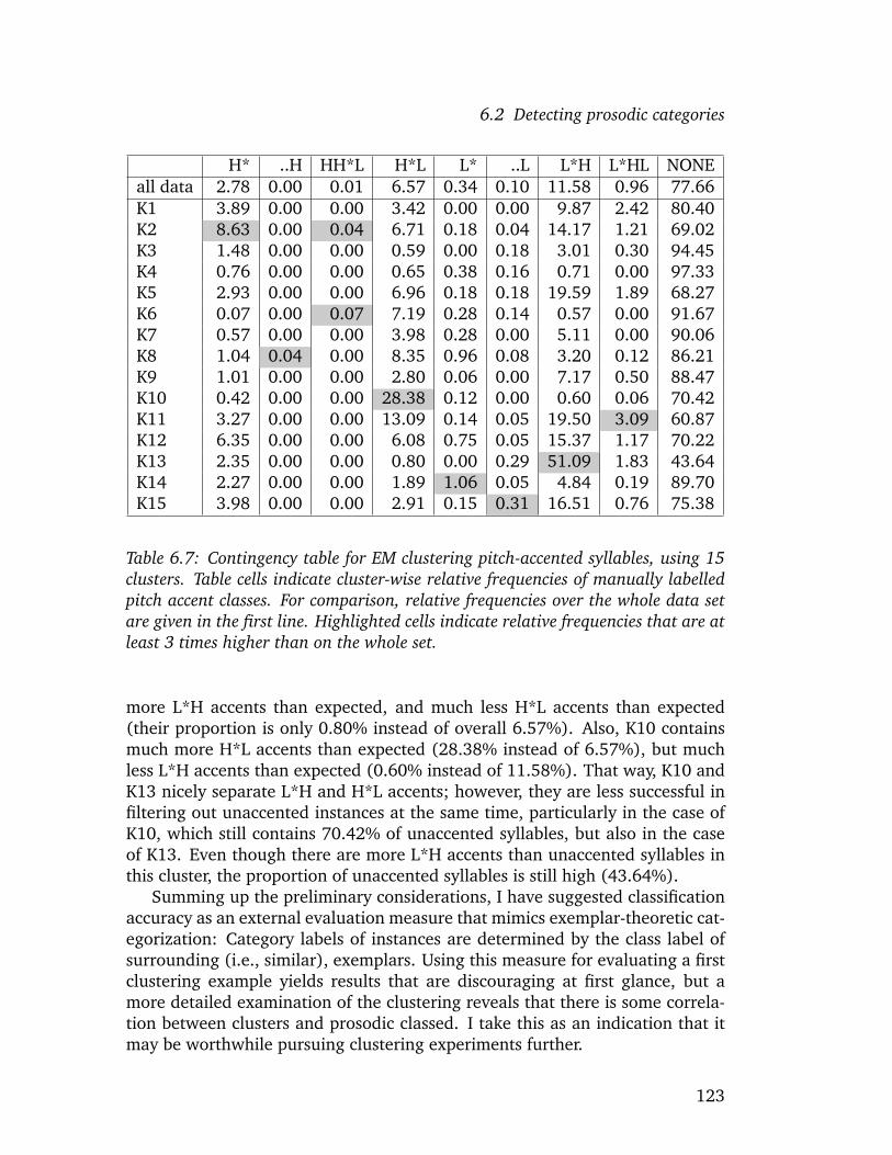
6.2 Detecting prosodic categories

H* ..H HH*L H*L L* ..L L*H L*HL NONEall data 2.78 0.00 0.01 6.57 0.34 0.10 11.58 0.96 77.66K1 3.89 0.00 0.00 3.42 0.00 0.00 9.87 2.42 80.40K2 8.63 0.00 0.04 6.71 0.18 0.04 14.17 1.21 69.02K3 1.48 0.00 0.00 0.59 0.00 0.18 3.01 0.30 94.45K4 0.76 0.00 0.00 0.65 0.38 0.16 0.71 0.00 97.33K5 2.93 0.00 0.00 6.96 0.18 0.18 19.59 1.89 68.27K6 0.07 0.00 0.07 7.19 0.28 0.14 0.57 0.00 91.67K7 0.57 0.00 0.00 3.98 0.28 0.00 5.11 0.00 90.06K8 1.04 0.04 0.00 8.35 0.96 0.08 3.20 0.12 86.21K9 1.01 0.00 0.00 2.80 0.06 0.00 7.17 0.50 88.47K10 0.42 0.00 0.00 28.38 0.12 0.00 0.60 0.06 70.42K11 3.27 0.00 0.00 13.09 0.14 0.05 19.50 3.09 60.87K12 6.35 0.00 0.00 6.08 0.75 0.05 15.37 1.17 70.22K13 2.35 0.00 0.00 0.80 0.00 0.29 51.09 1.83 43.64K14 2.27 0.00 0.00 1.89 1.06 0.05 4.84 0.19 89.70K15 3.98 0.00 0.00 2.91 0.15 0.31 16.51 0.76 75.38

Table 6.7: Contingency table for EM clustering pitch-accented syllables, using 15clusters. Table cells indicate cluster-wise relative frequencies of manually labelledpitch accent classes. For comparison, relative frequencies over the whole data setare given in the first line. Highlighted cells indicate relative frequencies that are atleast 3 times higher than on the whole set.

more L*H accents than expected, and much less H*L accents than expected(their proportion is only 0.80% instead of overall 6.57%). Also, K10 containsmuch more H*L accents than expected (28.38% instead of 6.57%), but muchless L*H accents than expected (0.60% instead of 11.58%). That way, K10 andK13 nicely separate L*H and H*L accents; however, they are less successful infiltering out unaccented instances at the same time, particularly in the case ofK10, which still contains 70.42% of unaccented syllables, but also in the caseof K13. Even though there are more L*H accents than unaccented syllables inthis cluster, the proportion of unaccented syllables is still high (43.64%).

Summing up the preliminary considerations, I have suggested classificationaccuracy as an external evaluation measure that mimics exemplar-theoretic cat-egorization: Category labels of instances are determined by the class label ofsurrounding (i.e., similar), exemplars. Using this measure for evaluating a firstclustering example yields results that are discouraging at first glance, but amore detailed examination of the clustering reveals that there is some correla-tion between clusters and prosodic classed. I take this as an indication that itmay be worthwhile pursuing clustering experiments further.

123

6.2 Detecting prosodic categories

6.2.2 A first experiment

As a first step, I have compared the classification accuracy in pitch accentclustering of six algorithms implemented in WEKA (Witten and Frank 2005),viz. Cobweb, DBScan, EM, FarthestFirst, OPTICS, and SimpleKMeans. WEKA’sHierarchicalClusterer could not be applied successfully due to memory limits.In most cases, the default settings suggested by WEKA were used, which is todetermine the appropriate number of clusters automatically. However, SimpleK-Means and FarthestFirst require specification of the desired number of clusters,and the default settings with only 2 clusters are clearly inappropriate. As afirst, straightforward approach the number of clusters was specified to be thenumber of prosodic categories, assuming as a first approximation that it willbe possible to identify one cluster for each prosodic category.14 In identifyingaccents, there are 8 different categories present in the SWMS data (cf. figure5.3), but two of them occur only twice, thus 6 clusters appeared to be the betterchoice.15

Figure 6.1 shows the results for the six algorithms in terms of classificationaccuracy. The baseline of 77.657% is indicated by the solid line. As stated aboveit is obtained by assigning each instance the overall most frequent prosodic classas its predicted label (”NONE” indicating no accent). Again, these results seemdiscouraging, as only two algorithms (Cobweb and DBScan) reach classifica-tion accuracy rates that are clearly above the baseline (85.687% and 82.142%,respectively). However, these two algorithms yield much higher numbers ofclusters than the other algorithms: Cobweb finds 3150 clusters, and DBScanfinds 237. The numbers of clusters are indicated inside the bars in figure 6.1.The other extreme is OPTICS clustering, with a degenerate single cluster con-taining all instances. For this case, the classification accuracy trivially corre-sponds to the baseline. EM clustering has identified 15 clusters, which seemsmore appropriate as the number of clusters is in the range of the number ofmanually determined prosodic classes.16

For FarthestFirst and SimpleKMeans clustering, the most frequent prosodicclass in each cluster was ”NONE”. Even though it is likely that in some of theseclusters some prosodic classes have made up a greater proportion of instancesthan on average, as was the case in the EM example above, there was no clusterwhere a single class was more frequent than the ”NONE” class, thus the resultsin both cases are equal to the baseline in terms of classification accuracy.

14Having discussed the EM clustering indicated in tables 6.6 and 6.7, it can be suspectedthat this assumption is too simple.

15One might even consider aiming at 5 clusters, since it is disputable whether the 26 in-stances of category ..L are sufficient. However, later on in this section, the question of appro-priate cluster numbers will be treated in more detail.

16The results of the EM algorithm in this experiment are actually the results discussed abovein more detail (tables 6.6 and 6.7).

124

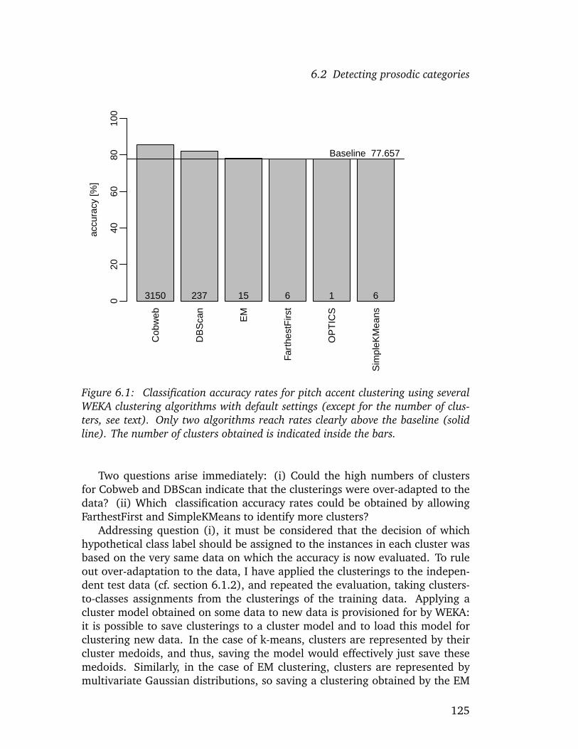
6.2 Detecting prosodic categories

Cob

web

DB

Sca

n

EM

Fart

hest

Firs

t

OP

TIC

S

Sim

pleK

Mea

ns

accu

racy

[%]

020

4060

8010

0

Baseline 77.657

3150 237 15 6 1 6

Figure 6.1: Classification accuracy rates for pitch accent clustering using severalWEKA clustering algorithms with default settings (except for the number of clus-ters, see text). Only two algorithms reach rates clearly above the baseline (solidline). The number of clusters obtained is indicated inside the bars.

Two questions arise immediately: (i) Could the high numbers of clustersfor Cobweb and DBScan indicate that the clusterings were over-adapted to thedata? (ii) Which classification accuracy rates could be obtained by allowingFarthestFirst and SimpleKMeans to identify more clusters?

Addressing question (i), it must be considered that the decision of whichhypothetical class label should be assigned to the instances in each cluster wasbased on the very same data on which the accuracy is now evaluated. To ruleout over-adaptation to the data, I have applied the clusterings to the indepen-dent test data (cf. section 6.1.2), and repeated the evaluation, taking clusters-to-classes assignments from the clusterings of the training data. Applying acluster model obtained on some data to new data is provisioned for by WEKA:it is possible to save clusterings to a cluster model and to load this model forclustering new data. In the case of k-means, clusters are represented by theircluster medoids, and thus, saving the model would effectively just save thesemedoids. Similarly, in the case of EM clustering, clusters are represented bymultivariate Gaussian distributions, so saving a clustering obtained by the EM

125

6.2 Detecting prosodic categories

algorithm would result in saving the distribution for each cluster. In any case,unseen instances from a new data set can be assigned to the clusters based onthe saved model: in the case of k-means clustering for instance, the pertinentcluster is determined by finding the closest medoid. In the case of EM cluster-ing, it is determined by finding the cluster to whose Gaussian distribution theinstance is most likely to belong to.17

The idea in using the classification accuracy measure given in definition 6.1above was to determine for each cluster a corresponding prosodic class. In thedefinition of the classification accuracy, the cluster-to-class correspondence wasdetermined by the majority class in each cluster. However, if the clusters rep-resent “real” categories, one would expect that the cluster-to-class correspon-dence should be the same on new data. In fact, this is a very desirable propertyin the context of my experiments — given that both clustering and cluster-to-class correspondence have been determined on independent data, applying theclustering to new data and evaluating it in terms of classification accuracy willassess its generalizability, and thus predict how useful the clusters are in cat-egorization. In evaluating the clusterings on new data, I therefore suggest tonot only keep the clustering, but also the cluster-to-class correspondence of theoriginal data, and to apply these in classifying new data. To my knowledge,this is a new evaluation method, and it necessitates redefining the classificationaccuracy measure to allow for independently determining the cluster-to-classcorrespondence.

The formal definition of the classification accuracy given in definition 6.1above can be replaced by definitions 6.2 and 6.3 below, which separate deter-mining the cluster-to-class correspondence from calculating the actual classifi-cation accuracy. For each cluster Ki the corresponding class can be determinedfrom contingency table a by finding the index of the most frequent class in thatcluster, i.e., the index of the corresponding class is the index k for which aik ismaximal. Since it could happen that several classes are equally frequent in acluster, we take the minimal index for which the maximum occurs from the setof indices for which aij is maximal, Li:

class(a, i) = min(Li) with Li = {k|aik = maxjaij}, 1 ≤ i ≤ N (6.2)

This way, the classification accuracy of a clustering applied to new data canbe determined in the following way. Let bij be the cells of contingency tableb obtained by applying the clustering to the new data, with bij calculated inanalogy to aij for instances from the new data. The classification accuracy forthe new data is then defined as

17Both algorithms are described in some more detail at the beginning of the following sec-tion.

126

6.2 Detecting prosodic categories

Cob

web

DB

Sca

n

EM

Fart

hest

Firs

t

OP

TIC

S

Sim

pleK

Mea

ns

accu

racy

[%]

020

4060

8010

0

Baseline 78.363

3150 237 15 6 1 6

Figure 6.2: Classification accuracy rates for pitch accent clustering using severalWEKA clustering algorithms with default settings, obtained on independent testdata. Here, the rates for Cobweb and DBScan have dropped below the baseline(solid line); for EM clustering, the results are again very slightly above the baseline,and FarthestFirst and SimpleKMeans clustering are still at the baseline. Again, thenumber of clusters obtained is indicated inside the bars.

class acc(b) =N∑

i=1

bi,class(a,i)∑Mj=1 bij

(6.3)

Here, the number of instances which are classified correctly is the numberof instances in the class determined by the clusters-to-class correspondence.The index of this class is class(a, i), and thus the number of instances whichare classified correctly is bi,class(a,i). Thus, the clusters-to-class correspondenceis determined from contingency table a, and the classification accuracy is de-termined from contingency table b using this correspondence. If b = a, i.e., ifthe classification accuracy is determined on the original data, definition 6.3 isequivalent to definition 6.1.

Re-evaluating the clusterings above on the independent test data in this wayyields the classification accuracy rates given in figure 6.2. Obviously, in the case

127

6.2 Detecting prosodic categories

of Cobweb and DBScan, the clustering was indeed too specific to the trainingdata—on the test data, the accuracy has dropped considerably below the base-line. This indicates that the clustering did not reveal “real” structure caused byregularities in the perceptual attributes of prosodic categories investigated herebut rather structure specific to that particular selection of data, including noise.

These results are rather discouraging: OPTICS has found only one degen-erate cluster, which yields baseline performance. Three algorithms (SimpleK-Means, FarthestFirst, and EM) perform only at or slightly above the baselinebecause in almost all clusters, unaccented syllables are more frequent than anyof the pitch accents. And the two algorithms which had identified more clus-ters, Cobweb and DBScan, despite performing clearly above the baseline on thetraining data, have obviously failed to capture generalizable regularities in therealization of prosodic categories—they now perform dramatically below thebaseline.

However, for EM, the minimal advantage over the baseline was stable whenthe cluster model was applied to new data. The results of the EM clusteringare the results discussed in more detail in the previous section (cf. tables 6.6and 6.7). As explicated there, this particular clustering did capture tonal as-pects, despite the fact that it performed approximately at the baseline, and itcan be suspected that the same is true for the FarthestFirst and SimpleKMeansclusterings.

Question (ii), which classification accuracy rates could be obtained by allow-ing FarthestFirst and SimpleKMeans to identify more clusters, is still relevant,even though it has turned out that the good classification accuracy rates of Cob-web and DBScan clustering did not carry over to new data. In the EM clusteringexample, the proportion of accents in the clusters varies, but the predominancein numbers of unaccented instances mostly prohibited clusters where accentsdominate. When increasing the number of clusters, the average size of the clus-ters will decrease, and it is conceivable that then clusters can emerge in whichthe unaccented instances are less dominant.

Whether increasing the number of clusters will improve the clustering re-sults will be addressed in the following section.

6.2.3 Varying numbers of clusters

To systematically assess the influence of the number of clusters on the clusteringresults, I have varied the number of clusters for FarthestFirst, SimpleKMeans,and EM clustering. These three algorithms are the only ones for which it waspossible in WEKA to specify the number of clusters manually. I will brieflysketch how the three algorithms are implemented in WEKA (Witten and Frank2005).

In SimpleKMeans clustering, k points from the data set are randomly chosen

128

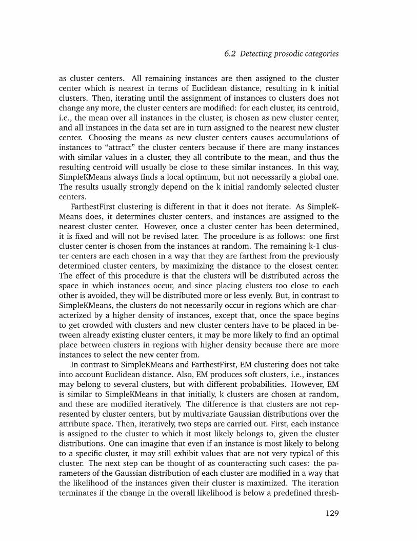
6.2 Detecting prosodic categories

as cluster centers. All remaining instances are then assigned to the clustercenter which is nearest in terms of Euclidean distance, resulting in k initialclusters. Then, iterating until the assignment of instances to clusters does notchange any more, the cluster centers are modified: for each cluster, its centroid,i.e., the mean over all instances in the cluster, is chosen as new cluster center,and all instances in the data set are in turn assigned to the nearest new clustercenter. Choosing the means as new cluster centers causes accumulations ofinstances to “attract” the cluster centers because if there are many instanceswith similar values in a cluster, they all contribute to the mean, and thus theresulting centroid will usually be close to these similar instances. In this way,SimpleKMeans always finds a local optimum, but not necessarily a global one.The results usually strongly depend on the k initial randomly selected clustercenters.

FarthestFirst clustering is different in that it does not iterate. As SimpleK-Means does, it determines cluster centers, and instances are assigned to thenearest cluster center. However, once a cluster center has been determined,it is fixed and will not be revised later. The procedure is as follows: one firstcluster center is chosen from the instances at random. The remaining k-1 clus-ter centers are each chosen in a way that they are farthest from the previouslydetermined cluster centers, by maximizing the distance to the closest center.The effect of this procedure is that the clusters will be distributed across thespace in which instances occur, and since placing clusters too close to eachother is avoided, they will be distributed more or less evenly. But, in contrast toSimpleKMeans, the clusters do not necessarily occur in regions which are char-acterized by a higher density of instances, except that, once the space beginsto get crowded with clusters and new cluster centers have to be placed in be-tween already existing cluster centers, it may be more likely to find an optimalplace between clusters in regions with higher density because there are moreinstances to select the new center from.

In contrast to SimpleKMeans and FarthestFirst, EM clustering does not takeinto account Euclidean distance. Also, EM produces soft clusters, i.e., instancesmay belong to several clusters, but with different probabilities. However, EMis similar to SimpleKMeans in that initially, k clusters are chosen at random,and these are modified iteratively. The difference is that clusters are not rep-resented by cluster centers, but by multivariate Gaussian distributions over theattribute space. Then, iteratively, two steps are carried out. First, each instanceis assigned to the cluster to which it most likely belongs to, given the clusterdistributions. One can imagine that even if an instance is most likely to belongto a specific cluster, it may still exhibit values that are not very typical of thiscluster. The next step can be thought of as counteracting such cases: the pa-rameters of the Gaussian distribution of each cluster are modified in a way thatthe likelihood of the instances given their cluster is maximized. The iterationterminates if the change in the overall likelihood is below a predefined thresh-

129

6.2 Detecting prosodic categories

old. In EM clustering, regions with higher density will correspond to peaks inthe Gaussian distributions of the clusters, otherwise, their likelihood would notbe maximal.

While for SimpleKMeans and FarthestFirst clustering, the clusters can bethought of as regions around cluster centers which stretch in each dimensionhalf-way to the next cluster center, the clusters in EM clustering have “softborders”, and the parameters of their Gaussian distribution determine how farthe cluster stretches in each dimension. Since in multivariate Gaussians, thevariances along each dimension are specified independently of the other di-mensions, clusters in EM clustering may stretch quite far in one dimension, butmuch less so in another dimension. I will come back to this in the discussion insection 6.2.6.

Turning to the experiments carried out using the three algorithms sketchedabove, I have systematically varied the number of clusters from 5 to 300 clus-ters. I will refer to this experiment as the 300 clusters experiment. Figure 6.3gives the classification accuracies for all three algorithms, on training (upperpanel) and test data (lower panel), respectively. The baselines are indicated bythe dashed lines. As before, the baseline is obtained by assigning each instancethe “NONE” label. The baseline is slightly higher on the test data because thereare slightly more unaccented instances.

Clearly the best results are obtained by SimpleKMeans clustering (dark graycircles). Here, classification accuracy rates of more than 84% are obtained onboth training data and test data. As may have been expected, the classificationaccuracy increases with the number of clusters. However, for SimpleKMeansclustering, the increase seems to level off at around 200 clusters on the trainingdata, and at around 150 clusters on the test data. For FarthestFirst (light graysquares), a clear increase can be observed at close to 300 clusters; it is possiblethat this increase may continue beyond 300 clusters. However, given the resultsfor up to 300 clusters, it seems unlikely that FarthestFirst approaches the classi-fication accuracy of SimpleKMeans. The best rates for FarthestFirst are between82 and 83% both on training data and test data. Regarding the EM algorithm(black diamonds), its results are not as good as the ones for SimpleKMeans andFarthestFirst, and it can be noted that they seem less stable than for the othertwo algorithms: they are more “jumpy” than the others even for higher num-bers of clusters. Even for EM the results are clearly above the baseline now,approaching 81% on the training data when reaching cluster numbers of 300.This is better than the 78.18% obtained for 15 classes in the first experiment,where the number of clusters had been determined automatically by cross vali-dation.18 It should be noted however that for EM clustering, the results on the

18In the WEKA implementation of EM clustering, the optimal number of clusters is obtainedin the following way: first, the model parameters are determined starting with only one cluster.Then, iteratively, the number of clusters is increased by one if this increases the cross-validatedlog-likelihood of the data, otherwise, the current number of clusters is regarded as optimal.

130

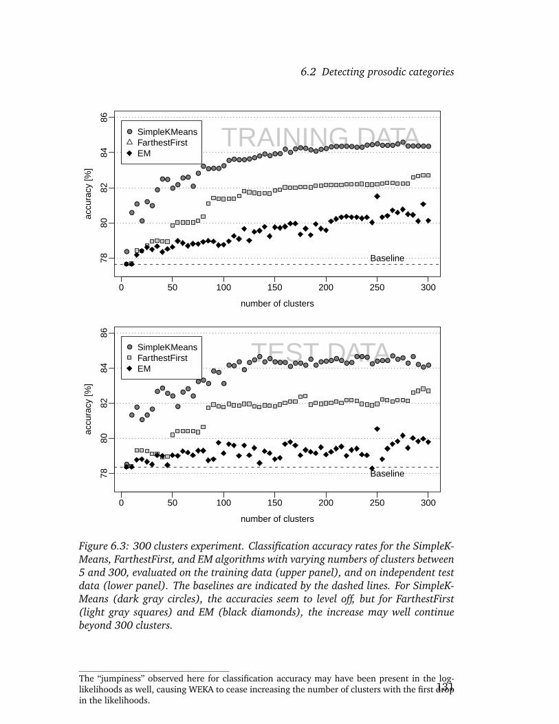
6.2 Detecting prosodic categories

0 50 100 150 200 250 300

7880

8284

86

number of clusters

accu

racy

[%]

TRAINING DATA●

●

●

●●●●●●●●●●

●

●●

●●●●●●●●

●

●●●●●●●●●●

●

●●●●●●●●●

●

●

●●

●●

●

●●

●

●

●●●●

● SimpleKMeansFarthestFirstEM

Baseline

0 50 100 150 200 250 300

7880

8284

86

number of clusters

accu

racy

[%]

TEST DATA●

●

●

●●

●

●●●

●●

●●

●

●●

●●●●

●●●●

●

●●●●●●●

●●●

●

●●

●●●

●

●●●

●

●●

●●

●

●

●●

●

●●●

●●

● SimpleKMeansFarthestFirstEM

Baseline

Figure 6.3: 300 clusters experiment. Classification accuracy rates for the SimpleK-Means, FarthestFirst, and EM algorithms with varying numbers of clusters between5 and 300, evaluated on the training data (upper panel), and on independent testdata (lower panel). The baselines are indicated by the dashed lines. For SimpleK-Means (dark gray circles), the accuracies seem to level off, but for FarthestFirst(light gray squares) and EM (black diamonds), the increase may well continuebeyond 300 clusters.

The “jumpiness” observed here for classification accuracy may have been present in the log-likelihoods as well, causing WEKA to cease increasing the number of clusters with the first dropin the likelihoods.

131

6.2 Detecting prosodic categories

test data are clearly below those reached on the training data.In summary, the accuracies obtained in the 300 clusters experiment show

that despite the first discouraging results, there is some potential in using clus-tering for detecting prosodic categories: if one takes the classification accuracymeasure introduced above to simulate exemplar-theoretic categorization accu-racy, it is a good sign that the results are clearly better than the baseline. Also, incontrast to the first experiment, all three algorithms have picked up regularitiesin the realization of prosodic categories that can be generalized to unseen in-stances. For SimpleKMeans and FarthestFirst, the classification accuracy scoreson the test data are in the same range as those on the training data, indicatingthat the clusterings generalize very well, while in the case of EM, lower scoreson the test data indicate that generalizability is limited. However, since thebaseline is slightly higher on the test data, this may have shed a slightly toofavorable light on the classification accuracy on the test data in all three cases.

Evaluating classification accuracy on new data is not a standard measure forexternal evaluation of clusterings, at least not to my knowledge. But particu-larly from an exemplar-theoretic perspective it is interesting because it resem-bles exemplar-theoretic categorization: there, new instances are categorizedby comparing them to exemplars stored in memory, and assigning them to thecategory which is most frequent in the neighborhood (cf. section 2.3.3). Here,new instances are categorized by assigning them to the category which is mostfrequent in their cluster, i.e., if the cluster is taken to represent the neighbor-hood, the proposed procedure models exemplar-theoretic categorization, andthe classification accuracy measures its performance.

A second aspect is that in the second part of this chapter (section 6.3), Iwill turn to predicting prosodic events using various classifiers. Against thatbackground it is of course desirable to evaluate how the clusters obtained herewould perform in prediction, compared to results that state-of-the-art classifierswould yield. In my opinion the most straightforward way of using the clusterresults for prediction is the procedure suggested above.

Still, before turning to further experiments and to the question whether in-creasing cluster numbers further would deserve some attention, I will introduceanother, more standard, evaluation measure than the classification accuracyused above.

6.2.4 Evaluation of clustering results

In many applications, there exists no manually or otherwise determined “cor-rect” grouping or “gold standard” which could serve to evaluate the clustering.In these cases, the goodness of the resulting clusters has to be evaluated us-ing internal criteria. For instance, the goodness of a cluster can be assessed bythe sum of squared errors between the cluster centroid and the objects in the

132

6.2 Detecting prosodic categories

cluster; or the goodness of classification of one particular object can be evalu-ated using its silhouette value (Kaufman and Rousseeuw 1990), which relatesthe distance of this object to other objects in the same cluster to its distance toobjects of other clusters.

If on the other hand, the correct assignment of instances to classes is known,as in the present application, an external evaluation is viable. In this case, theclustering can be evaluated by comparing the clusters to the correct, externallygiven, classes. In the present experiments, the externally given classes are theprosodic categories, which have been manually labelled. A variety of externalevaluation methods has been proposed in the literature. Recently, Rosenbergand Hirschberg (2007) have suggested the v-measure and demonstrated its ap-plicability, among others, on a pitch accent type clustering task very similarto the present task. They claim that, contrary to many other external mea-sures, v-measure is independent of the clustering algorithm or the data set, andindependent of the number of clusters found. The latter property makes v-measure appealing to the present application in that it is feasible to determinethe optimal number of clusters based on the v-measure scores. Also, given theindependence from data sets and cluster algorithms, and the similarity of thetwo applications, the scores obtained here can be compared to Rosenberg andHirschberg’s (2007) results for pitch accent type clustering. The difference tothe present task is that Rosenberg and Hirschberg (2007) classify only syllablesthat are known to be pitch-accented, while I want to obtain the classification aspitch-accented vs. unaccented from the clustering as well.

The v-measure is obtained by taking the harmonic mean of two scores whichrepresent desirable criteria in clustering applications. One score measures ho-mogeneity of the clustering. Homogeneity is satisfied if for each cluster, allmembers belong to the same class. The other score measures completeness,which is achieved if for each class, all instances that belong to this class areassigned to the same cluster. Homogeneity and completeness scores are im-plemented with reference to the conditional entropies of the class distributiongiven the clusters and that of the cluster distribution given the classes, respec-tively (Rosenberg and Hirschberg 2007, pp. 411–412).

For clustering pitch accents, Rosenberg and Hirschberg (2007) used datafrom the Boston Directions Corpus, which has been annotated according tothe ToBI labeling conventions for Standard American English (Silverman et al.1992). They mapped downstepped accents to their “normal” counterparts, ob-taining 5 classes of accent types. Similarly, as discussed in section 6.1.1, in thepresent experiments, I have used GToBI(S) labels, with the same mapping ofdownstepped accents, obtaining 8 classes of accents.

To get an idea of how the classification accuracy results discussed so farwould translate to v-measure results, I evaluated the first experiment againusing v-measure for evaluation (cf. figures 6.1 and 6.2 for the classification ac-curacy rates of these clusterings). The results are indicated in figure 6.4. This

133

6.2 Detecting prosodic categories

Cob

web

DB

Sca

n

EM

OP

TIC

S

Sim

pleK

Mea

ns

Fart

hest

Firs

t

v−m

easu

re

0.00

0.05

0.10

0.15

3150 237 15 1 6 6

training data

test data

Figure 6.4: v-measure results for pitch accent clustering on training data (darkgray bars) and on test data (light gray bars) using several WEKA clustering algo-rithms with default settings. The number of clusters obtained is indicated insidethe light gray bars.

time, results on training data and on test data are plotted next to each other indifferent shades of gray. The Cobweb algorithm yields the best results, as wasthe case for classification accuracy. Surprisingly for almost all algorithms theresults are better on the independent test data, i.e., when applying the modelobtained on the training data to the test data, v-measure is higher than on thetraining data itself. This effect is strongest for the Cobweb algorithm, eventhough a considerable drop had been observed in the classification accuracyscores for this algorithm when testing the clustering on the test data (cf. fig-ure 6.2). A small increase in v-measure could be argued to be expected sincethe test data contained a slightly higher proportion of unaccented syllables.Recall that v-measure combines two scores which measure homogeneity andcompleteness of the clusterings. Admittedly, homogeneity must increase witha more skewed distribution of classes in the dataset — perfect homogeneityis achieved if the class distribution in each cluster is skewed to a single class(cf. Rosenberg and Hirschberg 2007, p. 411). However, it is less clear whycompleteness should improve. But since the effect is quite strong in the case of

134

6.2 Detecting prosodic categories

Cobweb it is unlikely that it is only due to the improvement in homogeneity. Iwill discuss this effect in more detail below, arguing that it is an artificial effectwhich gets stronger with increasing number of clusters, and which arises whenevaluating the clusterings using less data for testing than for training.

As for DBScan, it can be seen that v-measure drops considerably on the testdata, confirming the effect found for classification accuracy, where the accu-racy had dropped below the baseline. The results for EM, SimpleKMeans, andFarthestFirst are comparable to the classification accuracy results—the three al-gorithms perform roughly in the same range. OPTICS, with its single cluster,is successfully singled out by a v-measure of 0. These results demonstrate thatv-measure is a more sensitive measure than the classification accuracy usedin the first experiment, where there were almost no differences between EM,SimpleKMeans, FarthestFirst, and the baseline.

Turning to the 300 clusters experiment (cf. figure 6.3 for the results in termsof classification accuracy), the results in terms of v-measure are presented infigure 6.5. Results on the training data are presented in the upper panel, andresults on the test data in the lower panel. Again, it can be observed that theresults in general are better on the test data than on the training data: the bestvalues of v-measure on the training data are around 0.12, while on the testdata, the best values are in the range between 0.14 and 0.15. The values on thetraining data are slightly lower than the values of v-measure obtained for pitchaccent clustering in Rosenberg and Hirschberg (2007), where values of approx-imately 0.125 to 0.13 were obtained for 100 clusters, and values of approxi-mately 0.175 for 300 clusters.19 It should be noted that their task was slightlydifferent from the task presented here, since only pitch-accented syllables wereclustered there, while I want the clustering to pick up not only differences inthe realization of pitch accents, but also differences between unaccented andpitch-accented syllables.

Returning to figure 6.5, while in terms of classification accuracy SimpleK-Means was clearly better than FarthestFirst, in terms of v-measure, this dependson the number of clusters. For up to about 80 clusters, SimpleKMeans (darkgray circles) is indeed better than FarthestFirst (light gray squares), both ontest data (upper panel) and training data (lower panel). Then, for up to about230 clusters on the training data, and for up to about 180 clusters on the testdata, SimpleKMeans and FarthestFirst are roughly comparable in terms of v-measure. For higher numbers of clusters, FarthestFirst performs better thanSimpleKMeans. On both test and training data, SimpleKMeans reaches a max-imum in v-measure at 150 clusters; for greater numbers of clusters, the valuesstart to decrease, while v-measure for FarthestFirst both on training and ontest data increases beyond 150 clusters, and possibly beyond 300 clusters. Thesame is true for EM (black diamonds)—while it does not reach the scores ob-

19v-measure results read off the diagram in Rosenberg and Hirschberg (2007, p. 418, fig. 5)

135

6.2 Detecting prosodic categories

0 50 100 150 200 250 300

0.04

0.06

0.08

0.10

0.12

0.14

number of clusters

v−m

easu

re

TRAINING DATA●●

●

●●●●●●●●

●●

●

●●●●●●●●●●● ●●●●●●●●●●●

●●●●●●●●●●

●●●●●

●

●●●●●●●●

● SimpleKMeansFarthestFirstEM

0 50 100 150 200 250 300

0.04

0.06

0.08

0.10

0.12

0.14

number of clusters

v−m

easu

re

TEST DATA

●●

●

●●●●●●●●●●

●

●●●●●●●●●●

●

●●●●●●●●●●

●●●●●●●●●●

●

●●●●●

●

●●●

●●●●●

● SimpleKMeansFarthestFirstEM

Figure 6.5: 300 clusters experiment. v-measure results for SimpleKMeans, Far-thestFirst, and EM algorithms with varying numbers of clusters between 5 and300, evaluated on the training data (upper panel), and on independent test data(lower panel). The v-measure scores seem to level off at around 150 clusters forSimpleKMeans (dark gray circles), but for FarthestFirst (light gray squares) andEM (black diamonds), the increase may well continue beyond 300 clusters.

136

6.2 Detecting prosodic categories

tained for FarthestFirst and SimpleKMeans at this point, its scores increase withthe number of clusters, and it cannot be said whether it could reach values ofv-measure in the same range as the other two algorithms.

Summarizing the v-measure results of this experiment, it can be stated thatfor SimpleKMeans clustering, a number of no more than 150 clusters seemsappropriate. However, for EM and FarthestFirst clustering, the results suggestthat even higher numbers of clusters might be of interest.

I thus ran a third experiment aiming at up to 3200 clusters, which will becalled the 3200 clusters experiment in the following. The results are presentedin figure 6.6. The results on the training data (upper panel) indicate that forSimpleKMeans and FarthestFirst clustering, allowing more clusters does notincrease v-measure further. For SimpleKMeans, the tendency observed alreadyin the 300 clusters experiment is confirmed: for numbers of clusters beyond150, there is no further increase in v-measure. For FarthestFirst clustering, thebest values obtained in the 300 clusters experiment were at 300 clusters, andthe results here show that this was an optimum even for up to 3200 clusters.In contrast, for EM clustering, the scores continuously but very slowly increase,possibly beyond 3200 clusters. The scores do no reach the scores obtained forSimpleKMeans and FarthestFirst, and since the increase seems to deceleratetowards the end, I take this to indicate that EM clustering will not outperformthe other two algorithms even for higher numbers of clusters.

For comparison, the v-measure for Cobweb clustering with its 3150 clusters(cf. figure 6.4) is indicated by the solid lines in figure 6.6. The lines are drawnfrom left to right across the whole diagram to allow for comparison to the re-sults of the other three algorithms for all numbers of clusters, even thoughtechnically, the Cobweb results should be indicated by just one data point at3150 clusters in each panel. For both FarthestFirst and SimpleKMeans, the op-timal results on the training data are very close to the Cobweb result. However,the optimal v-measure scores are obtained at much smaller numbers of clusters,viz. at around 150 and 300 clusters, respectively.

The v-measure results on the training data are in line with the classificationaccuracy results of the 300 clusters experiment presented so far: there, theaccuracy obtained on the test data had leveled off at approximately 150 clustersfor SimpleKMeans, and there had been a small increase at approximately 300clusters for FarthestFirst. However, so far I have only presented accuracy resultsup to 300 clusters; higher numbers of clusters may well yield better results interms of classification accuracy.

But turning to the lower panel in figure 6.6, when applying the clusteringsobtained on the training data to the test data, there is a continuous, slightincrease up to 3200 clusters for all three algorithms. This is surprising, at leastfor SimpleKMeans and FarthestFirst—why should the results for the test dataimprove even beyond the point where they stagnate for the training data? Also,the difference in v-measure between test data and training data approaches

137

6.2 Detecting prosodic categories

0 500 1000 1500 2000 2500 3000

0.04

0.06

0.08

0.10

0.12

0.14

0.16

number of clusters

v−m

easu

re

TRAINING DATA●

●●●● ●● ●●●●●●●●●●●●●●●●●●●●●●●●●●●●●●●●●●●●●●●●●●●●●●●●●●●●●●●●●●

Cobweb at 3150 clusters

● SimpleKMeansFarthestFirstEM

0 500 1000 1500 2000 2500 3000

0.06

0.08

0.10

0.12

0.14

0.16

number of clusters

v−m

easu

re

TEST DATA

●

●

●●●

●

●

●●●●●

●●●●●●●●●●●●●

●●●●●●●●●●●●●●●●●●●●●●●●●●●●●●●●●●●●●●●●

Cobweb at 3150 clusters

● SimpleKMeansFarthestFirstEM

Figure 6.6: 3200 clusters experiment. v-measure for up to 3200 clusters, evaluatedon the training data (upper panel), and on test data (lower panel). The horizontalsolid lines indicate values obtained for Cobweb clustering with 3150 clusters. ForSimpleKMeans (dark gray circles) and FarthestFirst (light gray squares), optimalresults on the training data are at 150 and 300 clusters, respectively. On the testdata, a continuous increase for all three algorithms can be observed.

138

6.2 Detecting prosodic categories

0.04 for the highest numbers of clusters, while it was at roughly 0.02 in the300 clusters experiment.

As explicated in the discussion of the v-measure results of the first experi-ment already, slight differences may have been attributed to slightly differentclass distributions in test and training data. But it is questionable whether dif-ferences in v-measure between training and test data in this order of magnitudecan arise solely from slightly different distributions. I will address this issue inthe following section.

6.2.5 Cross-validating the results

To rule out that the differences are only due to an unfortunate split into testand training data with different class distributions, I ran another experimentwith up to 3000 clusters for SimpleKMeans and FarthestFirst clustering, us-ing 10-fold cross validation. This will be referred to as the 3000X experiment.EM was not included because it takes a considerable amount of computationalresources even without cross-validation. Since the main interest in this experi-ment was not to compare different algorithms to one another but to investigatethe unexpected test vs. training data effect discovered above, leaving EM outhere was considered unproblematic, in particular since its results both in termsof v-measure and in terms of classification accuracy were inferior to those ofthe other two algorithms.

The procedure for evaluating clusterings in the 3000X experiment was asfollows. As described in section 6.1.2, the split into test and training data hadbeen based on file names—files ending on 1 made up the test set. Basing thesplit on file names ensures that data from the same utterance never end up bothin test and training set. I have kept to this principle and assigned the data to 10different bins, based on the digit on which the file name ended. In clustering, Ihave used the data of 9 bins as training data, holding out the data from one bin.The obtained clustering was evaluated on the training data (“validation”);20

then, the clustering was applied to the data from the remaining bin and theseresults were evaluated as well (cross-validation). This procedure was repeated10 times, holding out every bin once, resulting in an evaluation scheme thatmight be called 10-fold validation and cross-validation.21

The results are presented in figure 6.7. By and large, the results are similarto the results obtained in the simple validation procedure used above. Lookingat the validation results from the training data (upper panel), FarthestFirst issuperior to SimpleKMeans throughout. There is a little difference, however. In

20Usually, when using cross-validation, the results on the training data are not of interest;but they are relevant here to estimate the difference in performance on training vs. test data.

21It should be noted that since in each run, 9 out of 10 bins are used for training, the trainingsets in the 10 runs are never identical, but always overlapping. Only the test data are differentand non-overlapping in each run.

139

6.2 Detecting prosodic categories

●

●●

● ●

200 400 600 800 1000 1200 1400 1600 1800 2000 2200 2400 2600 2800 3000

0.11

0.12

0.13

0.14

0.15

0.16

0.17

number of clusters

v−m

easu

re

TRAINING DATA

●

●●

● ●

●

●● ●● ● ●●

SimpleKMeansFarthestFirst

●

●●

●

●●

●

●

●

●

200 400 600 800 1000 1200 1400 1600 1800 2000 2200 2400 2600 2800 3000

0.11

0.12

0.13

0.14

0.15

0.16

0.17

number of clusters

v−m

easu

re

TEST DATA

●

●●

●

●●

●

●

●

●

●

●●

SimpleKMeansFarthestFirst

Figure 6.7: 3000X experiment. Cross-validated v-measure values obtained by 10-fold validation and cross validation using 200 to 3000 clusters, on the trainingdata (upper panel), and on independent test data (lower panel). The boxes indi-cate the variation observed in each of the 10 folds. It can be seen that the differencein results on test and training data is present across all folds and increases withthe number of clusters.

140

6.2 Detecting prosodic categories

the simple validation case presented in figure 6.5, FarthestFirst and SimpleK-Means performed in the same range for cluster sizes between 150 and 250clusters. This is not the case here, where in the 200 clusters case, Farthest-First is better than SimpleKMeans for all 10 folds. The only difference in theclustering process was that the order of the input data has changed—due tosorting the instances according to the bins to which they belonged, which haschanged the initial cluster centers. This demonstrates how sensitive Farthest-First and SimpleKMeans can be to this initial choice. Anyway, in general thevalidation results on the training data in the upper panel are compatible withthe earlier results—FarthestFirst is better than SimpleKMeans, and the valuesof v-measure decrease from 200 to 400 clusters, which would not contradictthe earlier results which suggested that 300 clusters is optimal for FarthestFirst,and 150 clusters is optimal for SimpleKMeans.

But more importantly, the cross-validation results on independent test data(lower panel) confirm the earlier observation that the results are always betterthan the results on the training data: when comparing the boxes for the trainingdata in the upper panel with the boxes for the test data in the lower panel, itcan be observed that they never overlap: the effect is present across all folds.22

The effect is quite strong for higher numbers of clusters: while on the trainingdata, v-measure is very consistently slightly below 0.12 for SimpleKMeans andaround 0.125 for FarthestFirst for numbers of clusters beyond 1000, on the testdata, it is above 0.15 for cluster numbers beyond 1000 and even reaches 0.17for some folds with increasing number of clusters for both algorithms. Thisconfirms that the effect was not due to an unfortunate split into training andtest data—rather, it persists in 10-fold cross-validation.

I suggest that the effect is caused by using different amounts of data forevaluating the clusterings. About 10% of the data are used for testing, whileabout 90% are used for training. This entails that the clusters, which have beendetermined on the training data, are less dense in the testing case, i.e., on aver-age, there are fewer test instances in the clusters than training instances. Someclusters will not be populated by test instances at all. This disproportion isquite dramatic for numbers of clusters towards 3000: since the test set containsroughly 10% of altogether 28,000 instances, 2800 instances will be distributedto 3000 clusters, resulting in less than one instance per cluster on average. Thisshould result in very good scores for homogeneity: in case of clusters with onlyone instance, homogeneity is trivially satisfied. On the other hand, complete-ness is expected to deteriorate when the instances are distributed across manydifferent clusters. However, the completeness scores for the present data arevery low already—simply said, they cannot get much worse anyway. Since v-

22The results are also always more variable on the test data than on the training data, butthis is due to the fact that the training data are overlapping for the 10 folds, as mentionedabove in footnote 21.

141

6.2 Detecting prosodic categories

measure combines both scores, considerably increased homogeneity scores willmore than compensate for the slightly decreased completeness scores.

In order to show that the higher v-measure values on the test data are in-deed caused by evaluating the clusters on fewer instances than were in thetraining set, I repeated the experiment in two different settings. In one setting,I used only one bin for training, and the remaining 9 bins for testing, effec-tively reversing the training-test split from the 3000X experiment to have fewertraining data than test data. This experiment is called the 10:90 experiment inthe following. In the second setting, I have again used only one bin for train-ing, and only one other bin for testing, resulting in about the same amount oftraining and test data. This will be referred to as the 10:10 experiment.

The results for the 10:90 experiment, with less training data than test data,are presented in figure 6.8. At first glance, it can be seen that the evaluationresults seem exchanged. In evaluating the clusterings on the training data (up-per panel), v-measure increases with increasing numbers of clusters, which isthe trend that had been observed in evaluating on the test data in the 3000Xexperiment. When evaluating the clusterings on the test data (lower panel),v-measure is best for smaller numbers of clusters and then decreases with in-creasing numbers of clusters, as it had when evaluating on the training data inthe 3000X experiment.23

It is further interesting to note that not only are the trends for increasingnumbers of clusters exchanged when reversing the training-test split, but thescores are a little more extreme:24 In the 10:90 experiment, the scores on thetraining data resemble those obtained on the test data in the 3000X experiment,but they are slightly better. Vice versa, the scores on the test data in the 10:90experiment resemble those on the training data in the 3000X experiment, butthey are slightly worse.

This observation indicates that, while v-measure may be independent of theclustering algorithm, the numbers of clusters, and the data set, as Rosenbergand Hirschberg (2007) claim, it is obviously not independent of the size of thedata set. Thus, for the present application, in which testing on independentdata is interesting because generalizability to new data is desirable, the settingfor evaluation should be chosen in a way that the clusterings can be evaluatedusing the same amount of data for training and testing. This is what I have donein the 10:10 experiment, using one bin for training, and one bin for testing,resulting in roughly equal amounts of training and test data, each consisting ofapproximately 10% of the original data.

The results are given in figure 6.9. Evaluating on the training data (upper

23It can also be observed that the scores on the training data are more variable than thoseon the test data. This is because this time, there was no overlap between training data, butthere was an approximately 90% overlap in the test data, cf. footnote 21.

24The axes in figures 6.7 and 6.8 are identical to allow for direct comparison of the twodiagrams.

142

6.2 Detecting prosodic categories

●

200 400 600 800 1000 1200 1400 1600 1800 2000 2200 2400 2600 2800 3000

0.12

0.14

0.16

0.18

0.20

number of clusters

v−m

easu

re

TRAINING DATA

●

●

●

SimpleKMeansFarthestFirst

●

●●

●

● ●

●

●

●●● ●

200 400 600 800 1000 1200 1400 1600 1800 2000 2200 2400 2600 2800 3000

0.12

0.14

0.16

0.18

0.20

number of clusters

v−m

easu

re

TEST DATA

●

●●

●

● ●

●

●

●●● ●

●●

●

●

SimpleKMeansFarthestFirst

Figure 6.8: 10:90 experiment. Cross-validated v-measure values obtained by 10-fold validation and cross validation with 10% training and 90% test data. Theresults on the training data (upper panel) resemble those on the test data in the3000X experiment; results on the test data (lower panel) resemble those on thetraining data in the 3000X experiment.

143

6.2 Detecting prosodic categories

●

200 400 600 800 1000 1200 1400 1600 1800 2000 2200 2400 2600 2800 3000

0.13

0.14

0.15

0.16

0.17

0.18

0.19

number of clusters

v−m

easu

re

TRAINING DATA

●

●

●

SimpleKMeansFarthestFirst

●

●

●

● ●

200 400 600 800 1000 1200 1400 1600 1800 2000 2200 2400 2600 2800 3000

0.13

0.14

0.15

0.16

0.17

0.18

0.19

number of clusters

v−m

easu

re

TEST DATA

●

●

●

● ●●

●

●

●

● ●

SimpleKMeansFarthestFirst

Figure 6.9: 10:10 experiment. Cross-validated v-measure obtained by 10-foldvalidation and cross validation with 10% training and 10% test data. Results onthe training data (upper panel) and results on the test data (lower panel) indicatethat higher numbers of clusters are better.

144

6.2 Detecting prosodic categories

panel) yields results identical to the 10:90 experiment, since the training datawere identical. As stated before, the scores increase with the numbers of clus-ters. Looking a little closer, the best score of slightly more than 0.18 on averageis obtained at 2800 clusters, and there is no further increase for 3000 clusters.When evaluating the clusterings on the test data (lower panel), the results for200 clusters are only very slightly lower, indicating that the clusterings general-ize very well. Also, now the same trend as for the training data can be observed:the scores increase when increasing the number of clusters. However, the in-crease is smaller than on the training data, reaching an optimal value of about0.165 on average for 2800 clusters. Again, there is no further increase for 3000clusters. This indicates that the clusterings are not over-adapted to the train-ing data for numbers of clusters up to 2800, but that up to these numbers ofclusters, the clusterings have captured structure in the data that generalizes tonew data. However, the degree of generalization decreases with the number ofclusters.

These results obtained in the 10:10 setting indicate that up to 2800 clustersare optimal for both FarthestFirst and SimpleKMeans. The results in the 10:90setting (cf. figure 6.8) suggest that 200 clusters is optimal for both algorithms.However, in both cases, training data and obtained clusterings are identical. Ifone decides not to consider the results on the test data and to evaluate juston the training data instead, the 10:90 experiment, with less training data,indicates that high numbers of clusters of up to 2800 are optimal, while the90:10 experiment, with much more training data, suggests that 200 clustersare optimal. It is puzzling that for small amounts of training data, the bestscores are obtained for high numbers of clusters, while for large amounts oftraining data, the fewer clusters yield the best scores.

Thus, the results obtained using v-measure for evaluation are inconclusive.If my claim is right and it is not viable to compare v-scores obtained for differentamounts of data to each other, one can only determine the optimal number ofclusters depending on the amount of data. Unfortunately, then, it is not possibleto determine the optimal number of clusters for the large amount of trainingdata here, because of the lack of the same amount of test data. However, it maywell be that the small amount of training data is not sufficient to capture thegeneral structure of prosodic categories.

To assess whether the amount of training data in the 10:10 setting wassufficient to capture the structure of prosodic categories, I have returned tothe classification accuracy measure. This serves to get an idea of how wellclusterings obtained on a small training set could perform in categorization.I have calculated classification accuracy rates for the 10:10 setting as well asfor the 10:90 setting. The results for evaluating on the training data, whichare identical in both settings, are depicted in figure 6.10. It can be seen thatthe accuracies increase almost linearly with increasing numbers of clusters andreach 100% for 2800 and 3000 clusters, which is suspiciously perfect and must

145

6.2 Detecting prosodic categories

●

●

●●

200 400 600 800 1000 1200 1400 1600 1800 2000 2200 2400 2600 2800 3000

85

90

95

100

number of clusters

accu

racy

[%]

TRAINING DATA

●

●

●●

●●

SimpleKMeansFarthestFirst

Figure 6.10: 10:10 experiment. Classfication accuracies obtained by 10-foldvalidation using 200 to 3000 clusters, on training data corresponding to about10% of the original data. For higher numbers of clusters, accuracies of 100% orclose to 100% are reached, which very likely indicates over-adaptation to the data.

certainly be caused by over-adaptation to the data.Indeed, the classification accuracies for the test data in the 10:10 setting,

which are given in figure 6.11, are much less perfect. Results for the two algo-rithms are given in two separate panels because there was too much overlap.The results for SimpleKMeans (upper panel) indicate that 400 or possibly 600clusters are optimal in terms of classification accuracy, while for FarthestFirst(lower panel), 600, or possibly 1000 clusters are best. Comparing the two algo-rithms, SimpleKMeans is better than FarthestFirst. However, as can be seen, theresults are quite variable, which makes it hard to tell which number of clustersis definitely better than the rest. This variability can be reduced by using moredata for testing: for the 10:90 setting, compatible, but less variable results areobtained. These are presented in figure 6.12. Here, it can be said with moreconfidence that 600 clusters is optimal for both algorithms, and that the accu-racies in this case are slightly above 83% for SimpleKMeans and slightly below83% for FarthestFirst.

Recall from the beginning of this section that the accuracies obtained on thetest data when training on the full training set, without cross-validation, wereup to 84% and 83% for SimpleKMeans and FarthestFirst, respectively (cf. figure6.3). Given the variability observed in evaluating the 10-fold clusterings, it is

146

6.2 Detecting prosodic categories

●●●

200 400 600 800 1000 1200 1400 1600 1800 2000 2200 2400 2600 2800 3000

80

81

82

83

84

85

number of clusters

accu

racy

[%]

TEST DATA●●

●

SimpleKMeans

●

●

200 400 600 800 1000 1200 1400 1600 1800 2000 2200 2400 2600 2800 3000

80

81

82

83

84

85

number of clusters

accu

racy

[%]

TEST DATA

●

●

FarthestFirst

Figure 6.11: 10:10 setting. Classfication accuracies obtained on the test data by10-fold cross-validation using 200 to 3000 clusters, for SimpleKMeans clustering(upper panel) and FarthestFirst clustering (lower panel). Comparable amounts oftraining and test data were used, each corresponding to about 10% of the originaldata. Best results are obtained for 400-600 clusters in case of SimpleKMeans, andat 600 or 1000 clusters in case of FarthestFirst.

147

6.2 Detecting prosodic categories

●

●

●

● ●

●

200 400 600 800 1000 1200 1400 1600 1800 2000 2200 2400 2600 2800 3000

80

81

82

83

84

85

number of clusters

accu

racy

[%]

TEST DATA

●

●

●

● ●

●

SimpleKMeans

●

●

●

●●●

200 400 600 800 1000 1200 1400 1600 1800 2000 2200 2400 2600 2800 3000

80

81

82

83

84

85

number of clusters

accu

racy

[%]

TEST DATA

●

●

●

●●●

FarthestFirst

Figure 6.12: 10:90 setting. Classfication accuracies obtained on the test data by10-fold cross-validation using 200 to 3000 clusters, for SimpleKMeans clustering(upper panel) and FarthestFirst clustering (lower panel). About 10% of the orig-inal data were used for training, and about 90% for testing. The results on thegreater amount are compatible with the earlier results, but clearer due to reducedvariability: 600 clusters are optimal for both algorithms.

148

6.2 Detecting prosodic categories

200 400 600 800 1000 1200 1400 1600 1800 2000 2200 2400 2600 2800 3000

82

83

84

85

86

87

88

number of clusters

accu

racy

[%]

TRAINING DATA

●

●

SimpleKMeansFarthestFirst

Figure 6.13: 90:10 setting. Classfication accuracies obtained by 10-fold valida-tion using 200 to 3000 clusters, on training data corresponding to about 90% ofthe original data. The accuracies increase with the number of clusters.

hard to tell whether the classification accuracies obtained here on the smalltraining set are actually in the same range as the accuracies expected whentraining on the full set.

Since it is unproblematic to use different amounts of test and training datawhen using classification accuracy as an evaluation criterion, except for thegreater variability when using smaller amounts of test data, I have calculatedclassification accuracy rates for the 3000X experiment. Recall that the training-test split in this case was 90:10. The results on the training data are presentedin figure 6.13. In contrast to the 10:10 and 10:90 settings, the classificationaccuracies on the training data do not reach 100%. However, they increasecontinuously for higher numbers of clusters. The increase is not linear butdiminishes with increasing numbers of clusters.

The results on the test data are given in figure 6.14. Again, the results forSimpleKMeans and FarthestFirst are given in two panels because they overlap.Both algorithms reach accuracy rates of more than 85%,25 with slightly betterscores for SimpleKMeans. Also, SimpleKMeans reaches these values for fewernumbers of clusters, viz. for numbers of clusters around 1600. The best valuesfor FarthestFirst are obtained for around 2000 clusters.

25i.e., the median for the 10 folds is slightly higher than 85%

149

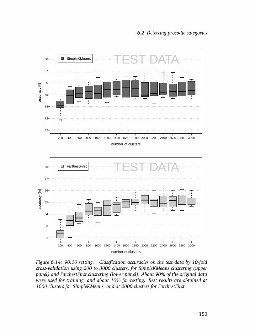
6.2 Detecting prosodic categories

●

200 400 600 800 1000 1200 1400 1600 1800 2000 2200 2400 2600 2800 3000

82

83

84

85

86

87

88

number of clusters

accu

racy

[%]

TEST DATA

●

SimpleKMeans

200 400 600 800 1000 1200 1400 1600 1800 2000 2200 2400 2600 2800 3000

82

83

84

85

86

87

88

number of clusters

accu

racy

[%]

TEST DATAFarthestFirst

Figure 6.14: 90:10 setting. Classfication accuracies on the test data by 10-foldcross-validation using 200 to 3000 clusters, for SimpleKMeans clustering (upperpanel) and FarthestFirst clustering (lower panel). About 90% of the original datawere used for training, and about 10% for testing. Best results are obtained at1600 clusters for SimpleKMeans, and at 2000 clusters for FarthestFirst.

150

6.2 Detecting prosodic categories

Summarizing the results of this section on cross-validation experiments, ac-cording to the classification accuracy scores, SimpleKMeans is slightly betterthan FarthestFirst. Also, for the amount of training data available here, around1600 clusters are optimal for SimpleKMeans, and around 2000 clusters areoptimal for FarthestFirst. Using these settings, classification accuracy rates ofaround 85% can be reached for pitch accent clustering. Using a small amountof training data, viz. only 10% of the full data set instead of 90%, the classifica-tion accuracy rates are lower, but not dramatically so, reaching approximately83%.

Using v-measure for evaluating the clusterings, the results are less homoge-nous. They indicate that for the larger amount of training data, around 200clusters are optimal, while for the small amount of training data, up to 3000clusters are best. Evaluating the clusterings using independent training data isproblematic because the amount of test data should match the amount of train-ing data. Thus, an evaluation on independent test data is not possible for thelarge amount of training data; however, for the small training set, evaluatingon independent test data confirms that up to 3000 clusters are optimal.

6.2.6 Discussion and Outlook

In this section, I have investigated clustering as a means to automatically detectprosodic categories in perceptual space. Given that all relevant perceptual di-mensions are known, it should be straightforward to detect clouds correspond-ing to phonetic categories using clustering techniques. In this vein, Pierrehum-bert (2003) reviews clustering results obtained by Kornai (1998) where clustersof F1/F2 data corresponded well to vowel categories. She posits that stable cat-egories are characterized by “well-defined clusters or peaks in phonetic space”(Pierrehumbert 2003, p. 210).

The experimental results presented in this section show that it is possibleto identify clusters which correspond well to prosodic categories. Usually inclustering, the goodness of this correspondence is determined by an externalevaluation measure which relates clusters to a gold standard, viz. the clustersto pitch accent classes in case of the experiments here. However, applyingthe v-measure (Rosenberg and Hirschberg 2007) as a standard measure wasproblematic because of its sensitivity to the amount of data, as elaborated insection 6.2.5. Instead, I have suggested to evaluate clusterings on independenttest data using the classification accuracy measure, which models exemplar-theoretic categorization: it assumes that all instances in a cluster belong to thesame pitch accent category, viz. the category with the highest likelihood in thatcluster. This way, each cluster will be assigned a pitch accent category, and newinstances can be categorized by determining to which cluster they belong.

Two clustering algorithms, namely SimpleKMeans and FarthestFirst, per-

151

6.2 Detecting prosodic categories

form similarly well with respect to this measure, reaching classification accura-cies of slightly more than 85% on independent test data. This is clearly abovethe baseline of around 78%. I will show in the following section using the samedata as in this section that prediction accuracies of approximately 87.5% can bereached when classifiers are specifically trained to predict pitch accents. Giventhat in the clustering experiments presented here, the intention was to modelhuman categorization by using classification accuracy, rather than finding theoptimal classifier for prediction in general, the 85% classification accuracy ob-tained here compares well to the overall optimum of 87.5%.

As for the number of clusters, these scores are reached for approximately1600 clusters in case of SimpleKMeans, and for approximately 2000 clusters incase of FarthestFirst, suggesting that these are appropriate numbers of clusters.Such high numbers of clusters may be unexpected at first. However, a one-to-one correspondence of clusters to phonetic categories cannot be expected. Forinstance, as Pierrehumbert (2003) points out, there may be overlap betweendistributions for different phonemes in different contexts, such as the overlapof devoiced /z/ realizations with “real” /s/ realizations. She states:

Cases such as these mean that parametric distributions forphonemes are not always well distinguished from each other, if theyare tabulated without regard to context. Within each given con-text, the distributions are much better distinguished. Thus, posi-tional allophones appear to be a more viable level of abstraction forthe phonetic encoding system than phonemes in the classic sense.(Pierrehumbert 2003, p. 211).

There are two solutions to this problem. Solution one is to cluster data fromcomparable contexts only (i.e., tabulated with regard to context, in Pierrehum-bert’s (2003) terms). Then, the clusters should be sufficiently well-defined tobe detected automatically. However, this implies that the contexts that are sup-posed to be relevant have to be known beforehand. Solution two is to includecontextual information as additional dimensions.26 For instance, if voicing ofsubsequent phonemes is included as a dimension, this will help to separate/z/ realizations in devoicing contexts from /s/ realizations. By way of exam-ple from the prosodic data used here, it has been discussed in chapter 5 thatthe PaIntE parameter distributions for different prosodic events overlap eventhough they are often significantly different from one another. For instance, infigure 5.4 on page 81 the distribution of the b parameter (which quantifies F0peak alignment) for L*H accents is indicated by the green solid line. The distri-bution is bimodal, indicating that the F0 peak is located either in the accented

26To some extent, I have done this here, since I have used more attributes than the percep-tually motivated ones, even though doing so was motivated by the better results rather than bythis theoretical consideration.

152

6.2 Detecting prosodic categories

syllable (the first peak of the distribution) or on the next syllable (the secondpeak in the distribution). The distribution overlaps with the distribution forL*HL accents: if for L*H accents, the F0 peak is indeed on the accented sylla-ble, it is located at the same point where it is usually located for L*HL accents(the peak of the L*HL distribution is at the same point as the first peak of theL*H distribution). As discussed in section 5.1.1, the bimodal distribution arisesbecause L*H accents in word-final syllables have their peak at the earlier point,and word-internal L*H accents have their peak at the later point (cf. figure5.5)—one could say that there are two positional variants of L*H. Including theposition of the syllable in the word as a further dimension would help to keepthe two distributions separate, hopefully resulting in two clusters for these twopositional variants of L*H.

The attributes that I have used for clustering are described in section 6.1.1.There are altogether 33 attributes, of which 29 are used for pitch accent clus-tering here. Thus, the clusters are detected in a 29-dimensional space. If eachdimension served to split each lower-dimensional cluster in two, one would get229, i.e., more than 500 million, clusters. This is of course grossly exaggeratedand unrealistic, not least because training and test data together contain only28,000 syllables, which entails that it is simply impossible to obtain more than28,000 clusters. But above all, one would not expect that each dimension isrelevant for each cluster. For instance, the position of the syllable in the wordwas only relevant for L*H accents, thus this dimension should only serve tosplit L*H clusters in two and thus just add one cluster instead of doubling thenumber of detected clusters. Still, relative to the high dimensionality of theclustering space, 1600 to 2000 clusters seems more appropriate than it seemedat first.

The experiments presented in this chapter are a first step towards detect-ing prosodic categories using the parameters suggested above. There are manyquestions left open. Maybe the most immediate one of these is which of thedimensions really contribute to detecting the clusters. The three algorithmswhich were systematically used in this section are SimpleKMeans, FarthestFirst,and EM clustering. The former two use the Euclidean distance to find clustersof instances. However, all dimensions contribute to this distance with equalweight. Thus, adding dimensions which do not serve to distinguish clustersmay even have the opposite effect in that it adds to the Euclidean distance,weighting down the contribution of the other dimensions. This could obscuremeaningful clusters in the other dimensions. The EM algorithm on the otherhand represents clusters as probability distributions over the attribute space.These distributions are multivariate Gaussians, thus the clusters are character-ized by their means and variances along each dimension. Theoretically, EMclustering should be better suited for data sets which include irrelevant dimen-sions, because dimensions which are not important for a cluster could be char-acterized by high variance in that dimension, covering all possible values. In

153

6.2 Detecting prosodic categories

practice, however, it seems that these parameters are not correctly detected, asattested by the consistently lower classification accuracy scores observed for EMclustering as compared to SimpleKMeans and FarthestFirst.27 Thus, irrelevantdimensions are expected to be problematic, and possibly more problematic forEM clustering than for the other two algorithms. Identifying which dimensionsare irrelevant can be addressed using attribute selection methods. This is anissue which is also relevant for the classification experiments described in thefollowing section. I will therefore defer it to the general discussion in chapter7.

A related issue is whether values in more important dimensions should bescaled to have greater impact in determining the similarity of instances. Thisidea is not implausible; in the exemplar-theoretic framework, its effect can beinterpreted as increasing the attentional weights to certain aspects of the exem-plars. However, this would require that the relevance of each dimension mustbe quantified beforehand, possibly using attribute selection as suggested above.

A third question is how the clustering results could improve with cleanerdata. As mentioned in section 6.1.3, the data are noisy, and some improvementsin the PaIntE approximation process envisioned for the future, in particular animproved smoothing algorithm, are expected to reduce this noise. I assumethat this will also have a positive effect on the clustering results.

Not an open question, but a point worth mentioning, concerns the distribu-tion of pitch accent categories in the data. As stated before, it is heavily skewed,especially so because of the overwhelming dominance of unaccented syllables.Such skewed distributions are often seen as disadvantageous for machine learn-ing schemes, and a common solution to this problem is to select only a subsetof the data with a more homogenous distribution. In this vein, Rosenberg andHirschberg (2007) have taken only a subset of the most frequent accents intheir data for clustering. However, not taking this option here was deliberatebecause the experiments aim at modeling human categorization, thus the datashould reflect “real-life” distributions rather than distributions that are optimalfor clustering. After all, humans manage to detect pitch accent categories de-spite the dominance of unaccented syllables.

Concluding this section on clustering pitch accents, the results in termsof classification accuracy are promising. For SimpleKMeans and 1600 clus-ters, cross-validated classification accuracies of between 84.6% and 86.5% arereached,28 or 85.5% on average. These are clearly above the baseline of be-tween 76.9% and 78.4%, or 77.7% on average. The baseline is the classifica-tion accuracy which would be obtained by predicting all instances to be “un-

27As mentioned above, I have used the default parameters for all algorithms tested here,except for the number of clusters, which was varied systematically. In case of EM clustering,there is a parameter restricting the number of iterations, and it defaults to 100 iterations. It ispossible that the EM results could be improved when allowing more iterations.

28Classfication accuracies and baselines vary for the ten folds.

154

6.3 Prediction of prosodic events

accented”. Furthermore, the accuracies compare well to those achieved in thefollowing section when training various classifiers to predict pitch accent cate-gories; for the best classifier, the averaged cross-validated prediction accuracywas 87.5% (cf. section 6.3.5), i.e., the best result was only 2% above the av-eraged accuracy obtained in SimpleKMeans clustering. In my opinion, theseresults are quite satisfactory, given that training classifiers for accent predictionis a supervised process, i.e. the correct labels are provided to guide construc-tion of the classifiers, while in the cluster-based prediction discussed here, thelabels are only used to determine the clusters-to-classes correspondence afterthe clusters have been detected.

The aim of clustering the data was to detect prosodic categories. This ambi-tion is dropped in training classifiers for prediction—even though the resultingclassifiers can be interpreted as partitioning the data space in some way, thesepartitions do not necessarily correspond to accumulations of instances, or toregions with higher density of instances. The following section will reveal howmuch can be gained in terms of accuracy in this case.

6.3 Prediction of prosodic events

The aim of this section is to model human categorization of prosodic eventsusing machine learning algorithms for classification.29 I have built classifiersfor both syllable-based accent and boundary prediction using the attributes dis-cussed above (cf. section 6.1.1). These attributes have been used for clusteringin the preceding section as well. The main interest in the prediction experi-ments is in how well automatically built classifiers can possibly perform thistask, particularly compared to human classification. The underlying idea is thatif the classifiers perform well, this corroborates my claim that the attributes,which include PaIntE parameters and duration z-scores, capture the most im-portant perceptual aspects of prosodic events. Performance of the classifiersis measured in terms of prediction accuracy. As in the previous section, theaccuracy rate is the proportion of instances which are correctly classified by aclassifier. Thus, beyond evaluating the obtained classifiers, the results of theprediction experiments can be used to assess the performance of the clusteringexperiments presented in the previous section. A second, related question iswhether any learning scheme is more suitable for this problem than others, i.e.,whether classifiers built using a particular scheme classify syllable instanceswith better accuracy than other learning schemes. Third, the resulting classi-fiers are to be evaluated on data of another speaker in order to assess how wellspeaker-specific classifiers generalize to other speakers. Generalizability would

29The experiments discussed in this section have been published in Schweitzer and Mobius(2009).

155

6.3 Prediction of prosodic events

not only confirm that the classifiers capture aspects of prosodic events that arerelevant in perception in general, it would also allow the use of the classifiersfor automatic prosodic annotation.

This section is organized as follows: I will sketch the procedure in section6.3.1 and the evaluation method in section 6.3.2. The evaluation results arepresented in section 6.3.3. Section 6.3.4 will address how the resulting classi-fiers generalize to data from another speaker. The classifiers will be comparedto results of other studies and to human labeling in sections 6.3.5 and 6.3.6,and finally their application to automatic prosodic labeling is illustrated on ex-amples from the database in section 6.3.7. I will conclude this section on theprediction of prosodic events by a discussion including an outlook on futurework in section 6.3.8.

6.3.1 Procedure

Using the training part of the SWMS database as training data (cf. section6.1.2), I have applied various machine learning schemes implemented in theWEKA software (Witten and Frank 2005) to build classifiers for both syllable-based accent and boundary prediction, i.e. to build classifiers that decide on thevalue of the accent or boundary tone attribute of a syllable instance based onthe values observed for the remaining attributes (cf. section 6.1.1).

In order to compare the results of the experiments presented here to resultsof studies which just predict two classes of accent (no accent vs. accented) andtwo classes of boundaries (boundary vs. no boundary), classifiers for these two-class problems were trained in addition to the classifiers predicting the full setof pitch accents and boundaries.30 Except for one case (for IBk instance-basedlearning), the default parameters suggested by WEKA were used in building theclassifiers.31

For the experiments, I used the training set of the SWMS data. WEKA pro-vides a more sophisticated 10-fold stratified cross-validation for evaluating itsclassifiers than the one I have used in clustering in the previous section: thedata in each run is split into 10 folds which each contain approximately equal

30Even though the aim was to build classifiers that predict the full set of accents, many re-sulting classifiers effectively predict just the most frequent classes: obviously, the less frequentclasses cannot be predicted with enough confidence to make up for their lower a-priori proba-bilities. Still, in evaluating these classifiers, classification results are compared to the full set ofmanual labels.

31The default settings of the IBk learning scheme implemented in WEKA set the k parameterto 1. The k parameter determines the number of neighbors considered in classification of newinstances, and with k=1 this learning scheme is identical to the separate IB1 learning schemein WEKA. Therefore, k=30 was used instead. Also, per default attribute values are normalizedwith the IBk learning scheme. Since the z-scoring of the PaIntE and duration parameters al-ready introduces normalization, I have run the IBk scheme once using normalization and oncewithout any normalization.

156

6.3 Prediction of prosodic events

proportions of instances of all classes. In each run, 10 classifiers are built usingthe data of all but one fold, and each classifier is evaluated on the data of theremaining fold. The split into folds is randomized which means that it is dif-ferent for different runs, reducing the risk of incidentally choosing a split thatis advantageous for the evaluation. However, WEKA has no access to the genrethat a particular syllable belongs to nor to the order of recording (cf. 6.1.2),which means that the resulting split may be unbalanced in that respect. Also,originally adjacent syllables may end up in test and training set. Nevertheless,in order to have objective estimates of the accuracy of the resulting classifiers, itwas better to have WEKA execute several runs using different splits. By evaluat-ing the cross-validated classifiers once more afterwards on the test data, it canbe verified that the prediction accuracies reached on the randomized splits iscomparable to that reached on the test set, which confirms that the randomizedsplits do not spuriously improve prediction accuracies.

The SWMS test set had to be held out from the experiments completelybecause its utterances are identical to the test set of the SWRK data, on whichthe classifiers were to be evaluated later when assessing their generalizability.Using utterances from this set in building the classifiers would have violatedthe assumption of independence of the test set.

6.3.2 Syllable-based vs. word-based evaluation

When evaluating the classifiers, one question that arises is whether the eval-uation should be syllable-based or word-based. Looking at the data, which iscomposed of instances of syllables, the most straightforward way is to calcu-late the prediction accuracy syllable by syllable, as in evaluating the clusteringresults in the preceding section. However, as described in section 6.1.1 above,two attributes that are available in classification are the attributes stress, whichindicates whether the syllable is lexically stressed, and wordfin, which indi-cates whether the syllable is word-final. It is theoretically impossible for anunstressed syllable to carry a pitch accent—theory claims that pitch accents arerealized on lexically stressed syllables. The only exceptions in our data are (i)the very rare trail tones ..H and ..L, which are not pitch accents strictly speaking,but which count as accents here because they are possible values of the accentattribute, and (ii) syllables that have not been correctly labeled for word stress.Thus, the simple rule that syllables with values of 0 for the stress attributeshould be classified as unaccented is expected to be captured by most classi-fiers, and successful application of this rule will increase accuracy rates. Thesame can be said of the wordfin attribute: phrase boundaries in fluent speechwithout hesitations do not occur word-internally, and thus, the classifiers areexpected to classify syllables with values of 0 for the wordfin attribute as notphrase-final and thus belonging to class NONE. Again, accuracy rates should

157

6.3 Prediction of prosodic events

benefit from this simple rule.This can be confirmed by running WEKA’s attribute selection schemes:

wordfin is ranked among the 7 most predictive attributes when predictingboundaries, and so is stress when predicting accents. The latter is even rankedfirst by several selection methods.32 Thus it is undeniable that the two attributeswordfin and stress contribute to the accuracy of the resulting classifiers. How-ever, they are less interesting from a perceptual point of view in that they aredetermined by the linguistic context and reflect its lexical properties rather thanperceptually relevant acoustic aspects of the particular rendition of this context.

In order to assess the performance of the classifiers beyond these two simplerules, I have trained classifiers on data from which, for boundary classification,I have eliminated all word-internal syllable instances, and, for accent classifi-cation, I have eliminated all syllable instances which were lexically unstressed.Since in the annotation of the database, only one syllable per word is marked asstressed, this leaves only one syllable per word—the final syllable for boundaryclassification, and the stressed syllable for accent classification. Thus, accuracyrates obtained for classifiers on the original data can be interpreted as syllable-based accuracies, and accuracy rates obtained on the transformed data sets canbe interpreted as word-based accuracies. Accordingly, the underlying data setsare termed “syllable-based” data set and “word-based” data set in the following.This also allows for comparing the present results to many other studies whichonly report word-based measures of performance.

6.3.3 Results

All classification algorithms for which I am reporting results in this section havebeen evaluated in three runs using 10-fold cross-validation in each run. Thus,the accuracy rates correspond to averaged accuracy rates of 30 different clas-sifiers built from various splits of the SWMS training data. Separate classifierswere trained for classifying accents and boundaries, and for syllable-based andword-based data sets, thus, for each algorithm, 120 classifiers were built alto-gether.

Figure 6.15 is intended to give an impression of the performance of all thelearning schemes that I have experimented with. It presents the word-basedaccuracy rates of all classification schemes that are implemented in WEKA (ver-sion 3.4) and that were applicable to the present classification problem (to bemore exact, it presents the averaged accuracy rates of the classifiers built in the

32In assessing the contribution of an attribute or a subset of attributes, I have applied sev-eral attribute selection methods implemented in WEKA including CfsSubsetEval, which selectsattributes based on their predictive ability taking into account possible redundancies betweenattributes, InfoGainAttributeEval, which measures the attributes’ information gain with respectto the class, and ChiSquaredAttributeEval, which assesses the attributes based on their chi-squared statistic with respect to the class.

158

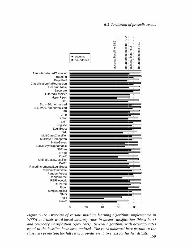
6.3 Prediction of prosodic events

ZeroRVFI

SMOSimpleLogistic

RidorREPTree

RBFNetworkRandomTree

RandomForestRandomCommittee

RacedIncrementalLogitBoostPART

OrdinalClassClassifierOneRNNge

NBTreeNaiveBayesUpdateable

NaiveBayesMultilayerPerceptronMultiClassClassifier

LWLLogitBoost

LogisticLMT

KStarJRipJ48

IBk, k=30, not normalizedIBk, k=30, normalized

IB1HyperPipes

FilteredClassifierDecorate

DecisionTableClassificationViaRegression

BayesNetBagging

AttributeSelectedClassifier

0 20 40 60 80

accentsboundaries

acce

nts

base

line

58.2

boun

darie

s ba

selin

e 72

.2

acce

nts

best

78.

2

boun

darie

s be

st 8

8.2

Figure 6.15: Overview of various machine learning algorithms implemented inWEKA and their word-based accuracy rates in accent classification (black bars)and boundary classification (gray bars). Several algorithms with accuracy ratesequal to the baseline have been omitted. The rates indicated here pertain to theclassifiers predicting the full set of prosodic event. See text for further details.

159

6.3 Prediction of prosodic events

three runs mentioned above and thus gives an estimate of the accuracy ratethat can be expected when building a classifier using this particular scheme).The accuracy rates of the classifiers for accent classification are indicated byblack bars, those of the classifiers for boundary classification are indicated bygray bars. The rates pertain to the classifiers trained to predict the full set ofaccents or boundaries. The classifiers are listed in alphabetical order. To avoidconfusion, I have kept the original names of the algorithms from the WEKA im-plementation, even if they are admittedly somewhat cryptic. I will discuss someof the schemes in more detail below; a short description of all schemes can befound in the WEKA book (Witten and Frank 2005).

In figure 6.15, the vertical dashed lines represent the baselines (black foraccent classification, and gray for boundary classification). The baselines aredetermined as the word-based accuracy rates achieved by the ZeroR learningalgorithm, which are indicated at the very bottom of 6.15. The ZeroR classifierdoes not infer any “rules”, as indicated by its name, but just assigns all instancesthe most frequent class found in the training set and thus in a way can beinterpreted as providing the chance level. On average, the most frequent accentwas NONE with a proportion of approximately 58.2%, and the class NONEwas also the most frequent boundary tone class with approximately 72.2%.Thus, on average, one can reach accuracy rates of 58.2% and 72.2% for accentsand boundary tones, respectively, by just assigning each stressed syllable theclass NONE in case of accents, and by assigning each word-final syllable theclass NONE in case of boundaries. Several learning schemes achieved the sameaccuracy rates as the ZeroR classifiers, and these were left out in figure 6.15 inorder to save space.33

The two dotted lines indicate the best results obtained in terms of word-based accuracy—the black dotted line shows the best word-based accuracy inaccent classification, which was at 78.2%, and was obtained using the Clas-sificationViaRegression scheme; the gray dotted line indicates the best word-based accuracy for boundary tone classification, which was at 88.2%, and wasobtained by the RandomForest scheme.

Figure 6.15 illustrates that the best results are not due to one or few out-standing learning algorithms that are particularly suitable for the present data;rather, when providing the information coded in the attributes discussed above,one can reliably reach quite high accuracy rates using any of a variety of differ-ent learning algorithms.

The exact word-based accuracy rates of the best learning algorithms fromfigure 6.15 are listed in table 6.8. Accuracy rates are given both for the two-class problem and for predicting the full set of GToBI(S) labels. To assess

33The following learning schemes were left out: AdaBoostM1, ConjunctiveRule, CVParame-terSelection, DecisionStump, Grading, HyperPipes, MultiBoostAB, MultiScheme, OneR, Stack-ing, StackingC, Vote

160

6.3 Prediction of prosodic events

Table 6.8: Word-based accuracy rates for the best algorithms and the baseline (Ze-roR). Most accuracy rates are comparable to the rates obtained by the Random-Forest algorithm: only accuracy rates marked by * are statistically significantlyworse than the corresponding rate for the RandomForest algorithm.

Algorithmaccents boundaries

2-class full set 2-class full setBagging 86.19 78.08 93.33 88.00ClassificationViaRegression 85.49 78.17 *92.29 *87.41LMT 86.24 77.54 93.37 87.84RandomForest 86.17 78.04 93.31 88.16ZeroR *58.30 *58.23 *72.16 *72.16

whether any of the algorithms is better than the rest, the asterisks indicatewhich classifiers performed significantly worse than the RandomForest classi-fiers. The RandomForest classifiers were chosen as a reference here becausethey performed best for the boundary tones and were also among the bestclassifiers for accents. It can be seen that these classifiers perform similarlywell. When predicting the full set of boundary tones, RandomForest classi-fiers with an accuracy of 88.16% were slightly ahead of the Bagging (88.00%)and LMT (87.84%) classifiers, while, when predicting the 2-class set, LMT per-formed best (93.37% vs. 93.33% for Bagging and 93.31% for RandomForest).However, all three performed similarly well, with no significant differences inaccuracy rates between RandomForest classifiers and those obtained using theother two schemes. The ClassificationViaRegression classifiers, however, wereslightly, but significantly, worse than the RandomForest ones. When predictingthe full set of accents, the accuracy rates ranged between 78.17% (Classifica-tionViaRegression) and 77.54% (LMT), with no significant difference betweenRandomForest classifiers and those built using any of the other three learningalgorithms. In predicting the two-class set of accents, the order was almostreversed, with LMT best at 86.24%, and Classification via Regression worst(among these top four) at 85.49%. Again, there were no significant differencesbetween RandomForest classifiers and those trained using any of the other threelearning algorithms.

It is not feasible in the scope of this thesis to investigate what exactly makesthe four best schemes best for the data here. However, I will briefly discusssome thoughts on this in the following paragraphs. Two of these best fourschemes above are actually very similar, viz. the Bagging and RandomForestschemes. The idea in bagging is to train an ensemble of several classifiers onrandom samples of the training data, and to let them “vote” for the predictedclass, taking the majority vote as the prediction of the ensemble. The Random-

161

6.3 Prediction of prosodic events

Forest classifier implemented in WEKA bags several RandomTree classifiers, i.e.,it is actually an instance of bagging as well. In contrast, the Bagging classifierin WEKA by default bags REPTree classifiers. Thus what is referred to as Bag-ging in the tables and figures above corresponds to bagged REPTree classifiers,and what is referred to as RandomForest corresponds to bagged RandomTreeclassifiers. The WEKA book (Witten and Frank 2005, pp. 316–317) notes thatinducing decision trees is an unstable process which is very susceptible to smallchanges in the training data, thus the single trees trained on different randomsamples of the data are expected to be very different. According to Witten andFrank (2005), this has the effect that the ensemble classifier is usually moreaccurate than a single one trained on the full training data. This is confirmedin case of Bagging and RandomForest here: both a single REPTree and a singleRandomTree perform clearly worse for the current tasks, as can be seen in fig-ure 6.15. Intuitively, the benefit in bagging is that each classifier in the ensem-ble will focus on different aspects of the data with more or less emphasis, dueto differently sampled training data, resulting in several “specialist” classifiersinstead of one that has to cover everything. In RandomForest classification, ad-ditional randomness is introduced in building the RandomTree classifiers whichare to be combined; here, only a random subset of attributes is considered whensplitting the tree, and no pruning is performed; in contrast, the REPTree classi-fiers which are combined in the default Bagging variant in WEKA are pruned,and all attributes are considered when building them. Despite the differencesin building the classifiers, the difference in performance between Bagging andRandomForest was negligible in the experiments here.

LMT and ClassificationViaRegression are similar in that they both apply re-gression models to a classification problem. LMT, which is abbreviated for Lo-gistic Model Trees, builds a model tree with additive linear logistic models atthe leaves. Similar to bagging, the models at the leaves combine several logis-tic regression models to contribute in prediction. However, classification is notbased on a majority vote; instead, the results of all models in the ensemble areadded in calculating the final classification result. The contributing models arebuilt iteratively, with each new model maximizing the likelihood of the trainingdata given the ensemble classifier. ClassificationViaRegression transforms theclasses into binary attributes and builds a model tree for each of them. How-ever, these trees have linear regression models at their leaves instead of logisticones.

It is not surprising that several of the best models here are ensembles ofclassifiers, since these are currently state-of-the-art and have often proven tobe superior to traditional, single classifier models. There are several techniquesto create ensemble classifiers, for instance bagging, boosting, and randomiza-tion. As stated in section 6.1.3, a characteristic of the data is that they are quitenoisy. Dietterich (2000) claims that bagging schemes are particularly suitablefor noisy data, in that bagging is superior to boosting and often to randomiza-

162

6.3 Prediction of prosodic events

Table 6.9: Word-based accuracy rates for instance-based learning with and withoutnormalization, using 30 neighbors compared to the best algorithms. Gray cellsindicate which version of IBk turned out better for the particular problem.

Algorithmaccents boundaries

2-class full set 2-class full setIBk no norm 84.57 76.96 91.77 87.22IBk norm 84.44 75.92 93.23 87.65Bagging 86.19 78.08 93.33 88.00ClassificationViaRegression 85.49 78.17 92.29 87.41LMT 86.24 77.54 93.37 87.84RandomForest 86.17 78.04 93.31 88.16

tion for such data. Obviously, this claim is supported here.As for the good results of LMT, I suggest that LMT can be interpreted as

partitioning the instance space into regions, as any decision tree does—leavescorrespond to regions defined by the attribute values along the path from theroot to the leave. However, classical decision trees then always predict the sameclass for all instances within the regions defined by the leave. LMT, on the otherhand, models the class distribution in each of these regions separately, allowingfor much finer distinctions.

A further learning scheme worth mentioning here is IBk, which is short forinstance-based learning. Instance-based learning is a so-called “lazy learning”scheme because no model is induced in training; rather, the data itself rep-resents the model. For prediction, new instances are compared to instancesfrom the training data using a distance metric, and the predicted class is theclass observed most often among the k closest neighbors of the new instance.I have experimented using 10, 20, and 30 neighbors for classification, with nodramatic differences in performance between the three. Table 6.9 lists the re-sults obtained for IBk using 30 neighbors, in comparison to the results of thebest algorithms, repeated from table 6.8. In WEKA’s implementation of IBk, it ispossible to specify whether the instances should be normalized or not. An inter-esting outcome of my experiments is that normalization proved to be beneficialin boundary classification, while using unnormalized data was better for pitchaccent classification, as indicated by the gray cells in table 6.9. As can be seen,the best results for IBk come close to the overall best results, however, thereis a small difference. IBk is particularly interesting from an exemplar-theoreticperspective because human categorization is claimed to work exactly that way(cf. section 2.3.3).

Summarizing this section, the classification results are very promising:when predicting the full set of accents or boundaries, prediction accuracies

163

6.3 Prediction of prosodic events

of the best classifiers are around 78% for pitch accents, which is 20% abovethe baseline, and around 88% for boundaries, i.e., 16% above the baseline.For the two-class problem, the accuracies are even higher, reaching 86% accu-racy for pitch accents (i.e., 28% above the baseline), and 93% for boundaries(i.e., 21% above the baseline). These best results are reached by several classi-fiers, with no significant differences between them. Also, many other learningschemes work almost as well, as illustrated by figure 6.15. Among these is theIBk learning scheme, which can be interpreted as modeling exemplar-theoreticcategorization. The next step in assessing the usefulness of the classifiers is tosee whether they generalize to data of other speakers. I will present first resultson this in the following section.

6.3.4 Generalizability

As a first step towards assessing the generalizability of the classifiers to otherdata, the best classifiers have been applied to the test set of the (female) SWRKdatabase. The results are comparable for boundaries: for instance, a Random-Forest classifier trained on the full SWMS training data reaches accuracy ratesof 88.9% on the SWMS test data and of 88.6% on the SWRK test data. Thus,applying classifiers built on the male data to the female data yields a drop inaveraged word-based accuracy of only 0.3%.

For pitch accents, performance is lower on the SWRK data: for instance, aRandomForest classifier trained on the full SWMS training data reaches accu-racy rates of 78.9% on the SWMS test data and of only 74.7% on the SWRK testdata corresponding to a drop in word-based accuracy of 4.2%. However, whenbuilding the classifier directly on the SWRK training data, the same accuracy of74.7% is reached on the SWRK test set. Thus, the RandomForest classifiers builtfrom the male SWMS training data are just as good in classifying the SWRK testdata as their SWRK counterparts. This demonstrates that the lower accuracy inapplying the SWMS pitch accent classifier is not due to unsatisfactory general-izability but rather is inherent to the SWRK data. On the contrary, the SWMSclassifiers perform just as well as the SWRK classifiers.

These results are very encouraging. Even though the two databases are verysimilar in that they were recorded from mostly identical text material, the twounderlying voices are not particularly similar—after all, one is a male voice,and one a female voice. Most attributes that were used for classification wererelated to F0 and temporal aspects, and the few attributes that were text-basedwere just rather abstract attributes derived from the text, but not, for instance,word identities, which would have been much more specific of a genre. Thenext step, in any case, will be to apply the classifiers to data of other speakers,with different material, which will hopefully confirm these expectations.

164

6.3 Prediction of prosodic events

6.3.5 Comparison with other studies

There are early studies on automatic classification of prosodic events (e.g.Wightman and Ostendorf 1994; Ross and Ostendorf 1996), which do not reachthe accuracy rates of more recent studies. Among the recent studies, Sridharet al. (2008) obtain word accuracy rates of 86.0% for the two-class problemof predicting pitch accents, and of 93.1% for predicting two classes of bound-ary tones, obtained on data from the Boston Radio News Corpus. These ac-curacies are slightly, but probably not significantly, lower than the best ratesachieved in my experiments, which for the two-class problem were obtainedby the LMT algorithm (86.24% and 93.37%, respectively). Similar results arereported by Hasegawa-Johnson et al. (2005), who obtain word-based accuracyrates of 84.2% and 93.0% for two-class pitch accent and boundary predictionon similar data. Comparing the results presented here to the results of thesetwo studies is relatively unproblematic because the data are similar: the twoclasses of pitch accents and boundary tones are derived from ToBI labels, andthe corpora both consist of news-style read speech by professional speakers.However, the corpora are from two different languages with different ToBI sys-tems.

Turning to German data, Zeißler et al. (2006) report accuracy rates of 77.0%for (two-class) pitch accent detection and of 88.6% for (two-class) boundarydetection for German data. This is significantly lower than the rates obtainedhere, but they classify spontaneous user interactions with a wizard-of-Oz systemand thus their data is very different from the data used here.

Another study reporting German results, which also predicts the full set of(English or German) ToBI labels instead of just two classes, is Braunschweiler(2006). He reports syllable-based accuracy rates of 65% and 60% for Ger-man and American English pitch accent classification, respectively, and syllable-based accuracy rates of 71% and 68% for German and American English bound-ary tone classification. I have only provided word-based accuracies in table 6.8above, because for the syllable-based data, I have not systematically evaluatedall algorithms in several runs. However, taking the RandomForest algorithm, forinstance, 10-fold cross-validation in one run yields estimated accuracy rates of87.5% and 93.9% on the syllable level for pitch accent and boundary tone clas-sification, respectively, using the full set in both cases. Thus, the present resultsare significantly better than the results reported by Braunschweiler (2006).

6.3.6 Comparison with human prosodic labeling

In order to assess the performance of the classifiers with regard to what couldmaximally be expected, it must be stated that manual prosodic labeling is no-torious for its subjectivity. Even human prosodic labelers are not perfect: ifseveral labelers label the same data prosodically, they usually do not perfectly

165

6.3 Prediction of prosodic events

agree with each other.Several studies (Pitrelli et al. 1994; Grice et al. 1996; Syrdal and McGory

2000) have assessed inter-labeler reliability in the ToBI labeling framework.Consistency between labelers in these studies is measured as the percentage ofequal transcriber-word pairs, with no claim as for which of the transcriptions iscorrect, i.e., these studies do not compare labeling results to a gold standard, asI do in the present experiments, instead they assess in how many instances thelabelers agreed. This makes it hard to relate the results to the current context,in which there are just two competing variants, viz. the gold standard and theautomatically generated prosodic transcription. In case of just two transcribers,the percentage of equal transcriber-word pairs is equivalent to the percentageof words for which the prediction was correct. However, the above measure ofinter-labeler reliability is intended to compare more than just two transcribers.For instance, Grice et al. (1996) compare results from 13 transcribers. If 12 ofthem agree, the percentage of equal transcriber-word pairs is only 84%, eventhough 12 out of 13 corresponds to a percentage of 92%. Thus, the inter-labeleragreement is a very stringent measure: if 92% of the labelers in a 13-labelerexperiment agree on a word, this yields an inter-labeler agreement of only 84%.If 11 out of 13 agree, i.e., 85%, and the two others agree with each other, theinter-labeler agreement is only 73%.

For German GToBI(S), Grice et al. (1996) report inter-labeler consistenciesof 70% for pitch accents, and of 86% for boundaries, and similar consisten-cies have been reported for English (Pitrelli et al. 1994; Syrdal and McGory2000). In comparison, the best results were around 78% accuracy for pitchaccents, and around 93% for boundaries. While these numbers look better atfirst glance, it should be kept in mind that a direct comparison is not validbecause the inter-labeler consistencies depend on the number of participants.Even though the present evaluation can be interpreted as comparing two label-ers, a human one and an automatic one, consistency experiments are intendedto include more than just two participants, but including more participants willalways decrease the consistency score.

6.3.7 Illustrating the results

I have implemented a prototype of an automatic prosodic labeling tool by com-bining the RandomForest classifiers obtained above with our German extension(IMS Festival 2010) of the Festival TTS system (Festival 2010). Festival cannot only synthesize utterances, it also provides tools to build utterance struc-tures automatically from speech label files, and these utterance structures canbe read and used by Festival. The prototype prosodic labeler thus reads in ut-terances from the database, derives the attributes needed for predicting pitchaccents and boundaries, and then lets WEKA predict them. The result is read

166

6.3 Prediction of prosodic events

into Festival for further processing; for instance, to generate prosodic label filesfor the utterance.

In order to give an impression of the performance of the classifiers for ac-cent and boundary prediction, I have used the prototype to generate prosodiclabel files for the first five utterances from the test data. The results are dis-played in screenshots of F0 contours and automatically generated label files infigures 6.16 to 6.19. Each example is accompanied by a table listing correctand predicted prosodic events word by word. The classifiers were the word-based RandomForest classifiers trained to predict the full set of pitch accentsand boundary tones. Even though the full set of boundaries was predicted,distinguishing between (H)% and H%, and between (L)% and L%, in generat-ing the label files, (L)% boundaries were mapped to L% boundaries, and (H)%boundaries were mapped to H% boundaries, thus, manual label files and pre-dicted label files in figures 6.16 to 6.19 differ in that respect. However, theunmapped predicted labels are listed in the corresponding tables.

There is one aspect in which the prototype’s results differ from the resultsobtained directly from the classifiers: IMS German Festival assumes that mono-syllabic function words are never stressed. However, word-based pitch accentprediction as described above is only carried out for the stressed syllable ofeach word; since there is no stressed syllable in monosyllabic function words,no prediction is generated for them. This is why in tables 6.10 to 6.14 monosyl-labic function words are left out. Given that there is not even one monosyllabicfunction word that is pitch-accented in our data, this is a reasonable procedure.However, the syllable-based classifiers might have predicted pitch accents forthese function words had they been stressed, and thus, the results presentedhere differ in this little detail from the results discussed above.

Results for the first utterance from the test data (“Das Zentrum blieb zumeistCardoso vorbehalten”, The center was mostly left to Cardoso) are presented intable 6.10, and a screenshot of the smoothed F0 contour and the correspond-ing label files is displayed in figure 6.16. The manually labeled accents andboundaries are indicated in the top tier, above the word tier. Predicted pitchaccents and boundaries are in two separate label files, which are displayed inthe two tiers below the word tier. The corresponding table 6.10 lists correctand predicted accents and boundaries, with prediction errors highlighted ingray. In this first example, there were only two incorrect predictions: the pitchaccent on rechts was missed; also, the intermediate phrase boundary after Zen-trum was not detected. It should be noted that the L*HL on Zentrum has beenpredicted correctly even though it is one of the less frequent accents. Thus,the example demonstrates that occasionally the less frequent accents can becorrectly predicted as well.

Figure 6.17 displays the results for the second utterance from the test set,f011 (“Beide Teams waren sehr motiviert und standig im Vorwartsgang, es warviel Tempo in der Partie”, Both teams were very motivated and always pushing

167

6.3 Prediction of prosodic events

accents boundariesword correct predicted correct predictedDas NONE NONEZentrum L*HL L*HL (L)- NONEblieb NONE NONE NONE NONEzumeist NONE NONE NONE NONECardoso H*L H*L NONE NONEvorbehalten NONE NONE (L)% (L)%weil NONE NONESporl L*H L*H NONE NONEsich NONE NONEdeutlich NONE NONE NONE NONErechts H*L NONE NONE NONEorientierte NONE NONE (L)% (L)%

Table 6.10: Correct and predicted pitch accents and boundaries in utterance f001,corresponding to the phrase “Das Zentrum blieb zumeist Cardoso vorbehalten”(“The center was mostly left to Cardoso”). For monosyllabic function words noaccents were predicted because they contain no stressed syllable by default in IMSFestival. Incorrect predictions are highlighted in gray.

forwards, there was much tempo to the match). Correct and predicted prosodicevents are indicated in table 6.11. There are several problems in this utter-ance, and it is certainly one of the more problematic cases from our database.Looking at the smoothed F0 contour in the middle of figure 6.17, the secondword in the utterance, monosyllabic Teams, is characterized by a strong risefollowed by a fall. It is classified as an H*L accent, which visually seems quiteplausible: the syllable ends where the intermediate phrase boundary is labeledin the manual label tier. Indeed, the contour is lower at that point than at thebeginning of the word. However, this is only because smoothing the F0 contourhas had the undesired effect of smoothing a clear rise into a peak: originally,the contour rose throughout the word Teams to the voiceless /s/ at the end.On the next word, waren, the contour is much lower. This can be verified bylooking at the raw F0 contour, which is displayed above the smoothed F0 con-tour. In smoothing, interpolation across the voiceless /s/, where no F0 frameswere present, turns the rise into a peak which is located where the voicelesspart started. Thus, smoothing here causes an H*L to be predicted where thereis only a rise towards a high boundary. The boundary tone on this word hasalso been incorrectly predicted—however, here, the predicted high intonationphrase boundary is much more plausible than the manually labeled intermedi-ate boundary, so this is a manual labeling error rather than a prediction error.The next two errors are on the word motiviert, and there is no obvious rea-

168

6.3 Prediction of prosodic events

Figu

re6.

16:

Pred

icti

onre

sult

for

utte

ranc

ef0

01fr

omth

ete

stse

t.Sp

eech

sign

alan

dsm

ooth

edF0

cont

our

are

indi

cate

dat

the

top;

the

labe

ltie

rsin

dica

tem

anua

llyla

bele

din

tona

tion

(top

tier

),w

ords

(2nd

tier

),pr

edic

ted

acce

nts

(3rd

tier

),an

dpr

edic

ted

boun

dary

tone

s(4

thti

er)

169

6.3 Prediction of prosodic events

accents boundariesword correct predicted correct predictedBeide L*H L*H NONE NONETeams NONE H*L (H)- H%waren NONE NONE NONE NONEsehr NONE NONE NONE NONEmotiviert L*H H* H% NONEund NONE NONEstandig NONE NONE NONE NONEim NONE NONEVorwartsgang H*L H*L (L)% (L)%es NONE NONEwar NONE NONEviel H* NONE NONETempo H*L NONE NONE NONEin NONE NONEder NONE NONEPartie NONE H*L (L)% (L)%

Table 6.11: Correct and predicted pitch accents and boundaries in utterance f011,corresponding to the phrase “Beide Teams waren sehr motiviert und standig imVorwartsgang, es war viel Tempo in der Partie” (“Both teams were very motivatedand always pushing forwards, there was much tempo to the match”). For mono-syllabic function words no accents were predicted because they contain no stressedsyllable by default in IMS Festival. Incorrect predictions are highlighted in gray.

son why these have been wrongly predicted. However, the next accent on theword viel is missed in prediction because viel has been mistakenly labeled asunstressed (in spite of being accented) and thus no prediction is made, whichis of course wrong here. The H*L accent on Tempo is also missed, which isprobably because the amplitude of the related peak is not too high—it can beseen that there are a lot of similarly vague “bumps” in the contour which indeeddo not correspond to accents. Finally, an H*L accent is predicted on the verylast word, which is not surprising because the contour is clearly falling there;however, this is due to the following boundary and not to a pitch accent. In myexperience from manual prosodic labeling, pitch accents at the very end of ut-terances are often not associated with clear F0 movements; it is easier to judgetheir accent status based on other parameters such as loudness, and then justdecide on the type of accent by the contour shape. Thus, adding parametersrelated to loudness might help in automatic classification as well in such cases.

Turning to the third utterance (“Bei Kaiserslautern agierte im Vergleich zurChampions League gegen Eindhoven Ramzy fur Koch als Manndecker”, In con-

170

6.3 Prediction of prosodic events

Figu

re6.

17:

Pred

icti

onre

sult

for

utte

ranc

ef0

11fr

omth

ete

stse

t.O

rigi

nala

ndsm

ooth

edF0

cont

ours

are

indi

cate

dat

the

top;

the

labe

lti

ers

indi

cate

man

ually

labe

led

into

nati

on(t

opti

er),

wor

ds(2

ndti

er),

pred

icte

dac

cent

s(3

rdti

er),

and

pred

icte

dbo

unda

ryto

nes

(4th

tier

)

171

6.3 Prediction of prosodic events

accents boundariesword correct predicted correct predictedBei NONE NONEKaiserslautern L*H L*H H% H%agierte L*H? NONE NONE NONEim NONE NONEVergleich L*H NONE NONE NONEzur NONE NONEChampions L*HL? L*H NONE NONELeague NONE NONE (H)- NONEgegen NONE NONE NONE NONEEindhoven L*H L*H (H)% H%Ramzy L*H L*H NONE (H)-fur NONE NONEKoch NONE NONE NONE NONEals NONE NONEManndecker H*L H*L (L)% (L)%

Table 6.12: Correct and predicted pitch accents and boundaries in utterance f021,corresponding to the phrase “Bei Kaiserslautern agierte im Vergleich zur Cham-pions League gegen Eindhoven Ramzy fur Koch als Manndecker” (“In contrast tothe Champions League match against Eindhoven, Ramzy was positioned to playman-for-man marking for Kaiserslautern”). For monosyllabic function words noaccents were predicted because they contain no stressed syllable by default in IMSFestival. Incorrect predictions are highlighted in gray.

trast to the Champions League match against Eindhoven, Ramzy was positionedto play man-for-man marking for Kaiserslautern), in table 6.12 and figure 6.18,for two of the incorrectly predicted pitch accents, the labeler had indicated un-certainty by the ? diacritic, indicating that these accents were problematic evenin manual labeling. Indeed, the amplitude of the pitch movement on agierte,which had been labeled L*H?, is not very pronounced, and even more so onVergleich—here, one may wonder if it was justified to manually label an L*H ac-cent given that there is almost no rise associated with the accent. Similarly, theamplitude of the movement on Champions, which should have been predictedL*HL, is smaller than usually observed for L*HL accents, which explains why ithas been mistaken for L*H. As for phrase boundaries, there were two mistakesinvolving intermediate boundaries; one was missed (on League), and one wasinserted (on Ramzy). However, the H% boundary predicted for Eindhoven mayeven be more justified than the (H)% boundary that had been labeled manually.

For the fourth utterance of the training data, the results are given in table6.13, but no screenshot is displayed because the utterance consists of a single

172

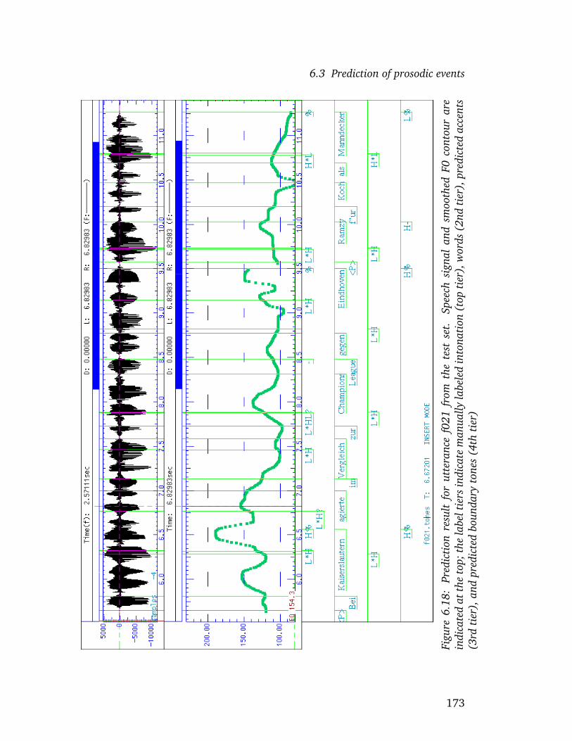
6.3 Prediction of prosodic events

Figu

re6.

18:

Pred

icti

onre

sult

for

utte

ranc

ef0

21fr

omth

ete

stse

t.Sp

eech

sign

alan

dsm

ooth

edF0

cont

our

are

indi

cate

dat

the

top;

the

labe

ltie

rsin

dica

tem

anua

llyla

bele

din

tona

tion

(top

tier

),w

ords

(2nd

tier

),pr

edic

ted

acce

nts

(3rd

tier

),an

dpr

edic

ted

boun

dary

tone

s(4

thti

er)

173

6.3 Prediction of prosodic events

accents boundariesword correct predicted correct predictedSchlusspfiff H*L H*L (L)% (L)%

Table 6.13: Correct and predicted pitch accents and boundaries in utterance f031,corresponding to the single-word phrase “Schlusspfiff” (“Final whistle”).

accents boundariesword correct predicted correct predictedNach NONE NONEeiner NONE NONE NONE NONEFlanke L*H L*H NONE (H)-von NONE NONEder NONE NONErechten NONE NONE NONE NONESeite L*H L*H (H)% H%kopft NONE NONE NONE NONEJuskowiak L*H NONE NONE (H)%nur NONE NONE NONE NONEZentimeter L*H L*H NONE NONEam NONE NONEFCN NONE NONE NONE NONETor NONE NONE NONE NONEvorbei H*L H*L (L)% (L)%

Table 6.14: Correct and predicted pitch accents and boundaries in utterancef041, corresponding to the phrase “Nach einer Flanke von der rechten Seite kopftJuskowiak nur Zentimeter am FCN Tor vorbei” (“Following a cross-path from theright side, Juskowiak’s header missed the FCN’s goal only by centimeters”). Formonosyllabic function words no accents were predicted because they contain nostressed syllable by default in IMS Festival. Incorrect predictions are highlighted ingray.

word (“Schlusspfiff”, Final whistle), and pitch accent as well as boundary tonehave been correctly predicted.

Finally, results for the fifth utterance (“Nach einer Flanke von der rechtenSeite kopft Juskowiak nur Zentimeter am FCN Tor vorbei”, Following a cross-pass from the right side, Juskowiak’s header missed the FCN’s goal only by cen-timeters) are indicated in table 6.14 and figure 6.19. There is only one errorin pitch accent prediction: the L*H accent on Juskowiak is missed. Turning tothe boundaries, in the first two cases, on the words Flanke and Seite, I would

174

6.3 Prediction of prosodic events

Figu

re6.

19:

Pred

icti

onre

sult

for

utte

ranc

ef0

41fr

omth

ete

stse

t.Sp

eech

sign

alan

dsm

ooth

edF0

cont

our

are

indi

cate

dat

the

top;

the

labe

ltie

rsin

dica

tem

anua

llyla

bele

din

tona

tion

(top

tier

),w

ords

(2nd

tier

),pr

edic

ted

acce

nts

(3rd

tier

),an

dpr

edic

ted

boun

dary

tone

s(4

thti

er)

175

6.3 Prediction of prosodic events

again claim that the predicted versions are probably better than the manuallabels: on Flanke, the contour rises throughout the word, continuing on thesecond, unstressed syllable. If there were no boundary following Flanke, onewould expect that the contour starts to fall on this second syllable already. OnSeite, the rise is characterized by a relatively high amplitude—this can be seenby comparing the rise on Seite to the rise on Juskowiak, for instance, which ismuch more typical of a (H)% boundary.

Summarizing these few examples, it can be said that prediction errors weresometimes caused by external factors and in these cases do not display weak-nesses of the classifiers themselves. For instance, in one case, F0 smoothinghad the undesired effect of turning a clear rise to the boundary into a peak,resulting in predicting an H*L accent. In one case, incorrectly labeled wordstress in the database has prevented prediction of a pitch accent for one word.In several cases, one might argue that the predicted labels are actually moresuitable than the manually labeled ones. These cases make up 8 out of 19 er-rors. They show that a considerable proportion of errors could be avoided if theinput data were more consistent. However, in “real-life” application, one can-not expect perfect input data, so such errors are almost certain to occur whenautomatically labeling new data.

Overall, the results of this prototype for automatic prosodic labeling arepromising. Even though there are some errors, many predictions are correct,and the errors are usually not blatant errors but in my experience are simi-lar to errors human labelers might make. In its current state, the prototype iscertainly useful in a bootstrapping approach when labeling new data, and I be-lieve that with some future improvement, it may even replace manual prosodiclabeling in some application scenarios.

6.3.8 Discussion and Outlook

In this section I have presented results on simulating prosodic categorizationusing machine learning methods to classify new exemplars. The results com-pare very well to results reported in other recent studies, particularly to resultson German. In contrast to most other studies, the classifiers predict the full setof GToBI(S) labels rather than just two classes. As illustrated in the precedingsection, they are good enough to be useful in automatic prosodic labeling.

Various learning schemes implemented in WEKA (Witten and Frank 2005)proved to be equally suitable for prosodic classification showing that good per-formance in classification is not necessarily due to one outstanding learning al-gorithm that is particularly suitable for the data; instead, this can be interpretedas showing that the information provided was sufficient to reliably reach quitehigh accuracy rates using various learning algorithms.

From an exemplar-theoretic point of view, it is interesting to note that

176

6.3 Prediction of prosodic events

instance-based learning performs almost as well as the best learning schemes.In instance-based learning, new instances are categorized based on their simi-larity to stored instances, assigning new instances the label which is most fre-quent among their neighbors in instance space. Exemplar-theoretic categoriza-tion has been claimed to work exactly this way (Lacerda 1995; Pierrehumbert2003). Johnson (1997) models exemplar-theoretic categorization slightly dif-ferently, but he himself notes that the process can be interpreted as “a sort of Knearest-neighbors classification” (Johnson 1997, p. 148).

I have also begun to assess the generalizability of classifiers trained on dataof one speaker to other speakers’ data. Results showed that the classifiers gen-eralize very well to similar data of another speaker in that they yield the sameaccuracy rates as classifiers trained directly on data of that speaker. Generaliz-ability is not only desirable in the context of automatic prosodic classification;I claim that the classifiers model human perception of prosodic categories byencoding perceptually relevant structure of prosodic categories, and in that re-spect, they are necessarily expected to generalize to other speakers: one wouldnot want to assume that different speakers encode prosodic categories differ-ently.

To further pursue the assessment of generalizability, the best classifiers willbe applied to data of more speakers in the future, in particular to data which donot match the training data so closely with respect to speech style or content.In the very near future, I will further develop the prototype to obtain a firstversion of an automatic labeling tool. The first challenge will be to apply thistool to spontaneous speech data in a new project on phonetic convergence inspontaneous speech. If on these data, similar accuracies can be reached asin the experiments presented here, the tool would constitute a very valuablecontribution to research on spontaneous speech. But even in its current state,the prototype is expected to be very useful in prosodically labeling new speechdata in a bootstrapping approach.

177

Chapter 7

Conclusion and Outlook

One aim of this thesis was to identify perceptual targets for prosodic events,extending Guenther and Perkell’s model (Guenther et al. 1998; Perkell et al.2001) from the segmental to the prosodic domain as explicated in section 2.3.5.This involves, first, identifying perceptually relevant prosodic dimensions, and,second, identifying which regions in the space spanned by these dimensionscan be considered as target regions for the different prosodic categories.

I suggest that temporal aspects in the realization of prosodic events are cap-tured in duration z-scores of segments and syllables. I have argued that thez-scores are a measure of “local” speech rate which is granular enough to cap-ture lengthening effects related to pitch accents and boundary tones. From anexemplar-theoretic perspective, the z-score of a speech unit duration can beinterpreted as the location of the exemplar in the temporal dimension of itsexemplar cloud. For instance, exemplars which lie at the center of their cloudin the temporal dimension exhibit a z-score of 0. As for the tonal aspects ofprosodic events, I suggest that properties such as peak alignment, peak height,and fall and rise amplitudes are relevant in perception, and that these proper-ties can be quantified by the PaIntE parameters. Thus, the PaIntE parameterscan be thought of as relevant dimensions in tonal perception.

Following Keating’s (1990) window model of coarticulation, it can be as-sumed that target windows for prosodic categories (the target regions, in Guen-ther and Perkell’s terms) are implicitly defined by the values observed for eachcategory. In this vein, I have shown in chapters 4 and 5 that for differentprosodic events the distributions of the parameters suggested above are oftensignificantly distinct from each other. However, it was also evident that there ismuch overlap between prosodic categories. The fact that the distributions aresignificantly different does not necessarily imply that they are different enoughfor discrimination. As Pierrehumbert (2003) states in discussing the distribu-tions of two categories:

178

Discrimination is not the same as statistical significance. As thequantity of data contributing to the distributions [...] increases to-ward infinity, the difference in the means of these distributions canbecome as statistically significant as one could wish. That is, [...]we can become more and more sure, scientifically speaking, thatthe distributions [...] are not the same. But no amount of certaintyon this point improves the situation with respect to discrimination ofthe categories when classifying an unknown incoming token” (Pier-rehumbert 2003, pp. 208–209).

In order to test whether the distributions are distinct enough for robustdiscrimination, I have carried out two sets of experiments: first, I have usedclustering as a means to automatically detect accumulations of similar sylla-ble instances corresponding to pitch accent categories, and second, I have builtclassifiers for predicting prosodic events. In both cases, PaIntE parameters aswell as duration z-scores were used as dimensions, but further attributes, whichwere mostly derived from these parameters, have been included. For instance,the PaIntE parameters and z-scores of surrounding syllables were included todistinguish local phenomena from more global phenomena. Local phenomenaare expected to be caused by prosodic events, while more global phenomenamay have no immediate linguistic function. For instance, high boundary tonesusually cause F0 rises that are confined to one or few syllables, i.e. they causea local rise, while more extended “global” rises in F0 are often due to inter-polation between events. Similarly, boundaries or pitch accents are expectedto locally lengthen syllable nuclei or syllable-final segments, while a slowerglobal speech rate would affect more than just one syllable. Also, some higherlinguistic properties were included to model speakers’ expectations, which arebased on the linguistic context in which a syllable occurs. For instance, speakerswould expect pitch accents on content words rather than on function words, orphrase boundaries at syntactic boundaries rather than within constituents.

The results indicate that the proposed dimensions do capture perceptualaspects of prosodic events. For instance, when evaluating the clusterings byassessing their prediction accuracy, scores of 85.5% can be reached for pitchaccents. Even higher accuracies are obtained in the prediction experiments;here, scores of 87.5% for pitch accents and of 93.9% for boundary tones canbe reached when evaluating the classifiers syllable by syllable.1 Given thateven human labelers do not reach 100%, as is evident from studies on labelerconsistency (Pitrelli et al. 1994; Grice et al. 1996; Syrdal and McGory 2000),these scores are encouraging.

Among the classifiers which yield the best scores there are several classifierswhich are based on decision trees. Similar to clustering, decision trees can

1The corresponding word-based accuracies are lower, at approx. 78% for pitch accents andat approx. 88% for boundaries when attempting to predict the full set of accents.

179

be thought of as partitioning the instance space: at each decision node, theinstance space is split in two, and instances in the two parts are treated by thetwo subtrees. The leaves then correspond to regions in instance space. Whenusing standard decision trees, all instances in these regions are predicted tobelong to the same class.2 In this way, standard decision trees identify regionsin instance space which correspond to the categories. Clustering, on the otherhand, detects categories by identifying regions in instance space with higherinstance density.

Thus, the clustering and prediction experiments can be seen as constitutingthe second step in applying Guenther and Perkell’s model (Guenther et al. 1998;Perkell et al. 2001) to the prosodic domain, by identifying target regions corre-sponding to the prosodic categories in the proposed perceptual space. However,the results of the clustering and prediction experiments indicate that there aremany target regions for each prosodic category: the clustering results indicatethat 1600 to 2000 clusters are appropriate for pitch accents. Similarly, in theprediction experiments, the best decision-tree based results were achieved bybagged decision trees. If standard decision trees constitute partitionings of theinstance space, then bagged decision trees are sets of trees which constitutedifferent partitionings, i.e., they identify no unique partitioning which relatesregions to classes, instead, they identify different partitionings which relate dif-ferent regions to different classes. In contrast, for standard decision trees (forinstance, J48, RandomTree, or REPTree in the WEKA implementation) thereis a 1-1 correspondence between the regions defined by the leaves and theclasses. However, these standard decision trees have been found to be infe-rior to the meta-trees cited above with respect to classification accuracy. Also,the trees that are obtained for these algorithms can be quite complex as well.For instance, a REPTree decision tree for pitch accent prediction with 10-foldcross-validated accuracy of 86.6%, i.e., 1% lower accuracy than the best algo-rithms, contained more than 500 leaves. A J48 tree with even lower accuracycontained almost 3000 leaves.

Clustering results and prediction results indicate that it is not possible toidentify one unique target region, in the sense of Guenther and Perkell, for eachprosodic category, at least not with the many dimensions currently used. How-ever, a convincing argument for their model is that disjoint target regions in ar-ticulator space are replaced by single convex target regions in perceptual space.Assuming many different target regions for each prosodic category would takemuch of the elegance of the model away. This perspective is also in oppositionto my earlier claim that the z-score and PaIntE parameter distributions can be

2This is not the case for some meta-learning algorithms which combine decision trees withother models. For instance, LMT and ClassificationViaRegression are decision trees with re-gression models at their leaves, as explained in section 6.3.3, i.e., they do not assume that allinstances in a particular region belong to the same class, however they assume that they can betreated using the same model.

180

seen as implicitly defining the target regions for the prosodic categories, as Ihad suggested in the concluding remarks in chapters 4 and 5.

Guenther et al. (1998) illustrate the concept of a single convex perceptualtarget region on the example of American English /r/ using F1 and F2 values asdimensions. However, to my knowledge the issue of discriminability betweendifferent segment categories in categorization is not addressed in their work.Indeed, the mean F1 and F2 values of American English /U/ vowels producedby female speakers and those of /3:/ vowels produced by either female or malespeakers found in a study by Hillenbrand et al. (1995) lie roughly in the targetregion posited for /r/. This indicates that when using only F1 and F2 as di-mensions, the target region for /r/ will not be distinct enough from the targetregions of these vowels to allow for discrimination, just as the target regionsfor prosodic events are not distinct enough when using only duration z-scoresand PaIntE parameters of the current syllable as dimensions.

I therefore suggest to regard the perceptual target regions in the sense ofGuenther et al. (1998) and Perkell et al. (2001) as very coarse, abstract percep-tual descriptions of the underlying targets of speech events. For the prosodicdomain, I maintain the view explicated in chapters 4 and 5: duration z-scoresand PaIntE parameters span a perceptual space in which these target regionsare located, and the distributions of values observed for each prosodic eventdefine its target region in this space. However, these target regions are overlap-ping and therefore not fine-grained enough for discrimination.

To allow for discrimination, context must be considered as well. As demon-strated by the clustering and prediction experiments in chapter 6, includingparameters which are mostly derived from the PaIntE and z-score parameters,such as the parameters of neighboring syllables, but also some higher-linguisticproperties, is sufficient to obtain very encouraging prediction accuracies, par-ticularly in relation to human labeler consistencies. This demonstrates that theparameters do capture most perceptually relevant properties.

However, some attributes may be irrelevant, and could artificially increasethe number of clusters or the complexity of the classifiers more than necessary.One way to gain some insight into the perceptual relevance of the attributesis to experiment with attribute selection methods. Such methods are providedwith WEKA (Witten and Frank 2005). I have not yet systematically looked atthis issue, but I have experimented somewhat with attribute selection whentraining the classifiers, reducing the number of attributes according to the rel-evance they were attested by WEKA’s attribute selection methods. However,different selection methods often yield different results, and the classificationresults were always worse when excluding attributes which had been judgedless relevant by some selection method. Still, systematic experiments couldserve to identify the most relevant dimensions. This could in turn then reducethe number of clusters or the complexity of the classifiers. However, I doubtthat the reduction in complexity will be enough to yield single convex target

181

regions for the prosodic events.There are other factors which in my opinion could help to reduce the com-

plexity of the clusterings. As stated in section 6.1.3, the data are noisy, andI hope to eliminate some of this noise in the future. One issue is that theF0 smoothing often has undesired effects, as discussed in sections 3.2.5 and6.3.7. A better F0 smoothing method, such as the one suggested by Reicheland Winkelmann (2010), could alleviate this problem. Some noise is also in-troduced by incorrect manual labelings – in illustrating the examples of auto-matically generated prosodic label files in 6.3.7, some instances were discussedfor which I claimed that the predicted label may have been more adequate thanthe manual label. Using more consistently labeled data, for instance data whereseveral labelers agreed, might help to assess the influence of such labeling er-rors.

To conclude, I will come back to the main contributions of this thesis, asthey were stated in the introduction. First, I have proposed that Guenther andPerkell’s speech production model for the segmental domain (Guenther 1995;Guenther et al. 1998; Perkell et al. 2001) can be applied to the prosodic domain,claiming that tonal and temporal aspects of the implementation of intonationcategories are phonemic settings. I have also pointed out that their model iscompatible with exemplar theory if it is assumed that the target regions areimplicitly defined by the exemplar clouds. Second, I have suggested that thePaIntE parameters as well as duration z-scores as a measure of local speechrate are the perceptual dimensions in applying Guenther and Perkell’s modelto the prosodic domain. Third, I have extensively investigated realizations ofGToBI(S) events in terms of these parameters, confirming that known effectson prosodic realization are visible in the parameter distributions. Fourth, Ihave conducted clustering experiments, in order to show that the suggesteddimensions are sufficient to detect prosodic categories. For evaluating the clus-terings, I have suggested an evaluation procedure which to my knowledge hasnot been used before, which aims at assessing the generalizability of cluster-ings. Finally, I have built classifiers to show that the suggested dimensions aregood enough to reach state-of-the art classification accuracies using supervisedmethods. Thus, a fifth, very valuable contribution of this thesis is a prototypeof a tool for automatic prosodic labeling, which will be improved further in thefuture.

182

Bibliography

Abney 1995 ABNEY, Steven P.: Chunks and dependencies: bringing pro-cessing evidence to bear on syntax. In: Computational Linguistics and theFoundations of Linguistic Theory. Stanford : CSLI, 1995

Baayen et al. 1995 BAAYEN, H. ; PIEPENBROCK, R. ; GULIKERS, L.: The CELEXlexical database—Release 2. CD-ROM. 1995. – Centre for Lexical Information,Max Planck Institute for Psycholinguistics, Nijmegen

Baayen 2001 BAAYEN, Harald: Word Frequency Distributions. Dordrecht :Kluwer, 2001

Barbisch et al. 2007 BARBISCH, Martin ; DOGIL, Grzegorz ; MOBIUS, Bernd ;SAUBERLICH, Bettina ; SCHWEITZER, Antje: Unit selection synthesis in theSmartWeb project. In: Proceedings of the 6th ISCA Workshop on Speech Syn-thesis (SSW-6, Bonn), 2007, pp. 304–309

Beckman and Ayers 1994 BECKMAN, Mary E. ; AYERS, Gayle M.: Guidelinesfor ToBI labelling, version 2.0. February 1994

Braunschweiler 2006 BRAUNSCHWEILER, Norbert: The Prosodizer — Auto-matic Prosodic Annotations of Speech Synthesis Databases. In: Proceedingsof Speech Prosody 2006 (Dresden), 2006

Browman and Goldstein 1986 BROWMAN, Catherine ; GOLDSTEIN, Louis:Towards an articulatory phonology. In: Phonology Yearbook 3 (1986),pp. 219–252

Browman and Goldstein 1992 BROWMAN, Catherine ; GOLDSTEIN, Louis:Articulatory phonology: an overview. In: Phonetica 49 (1992), pp. 155–180

Byrd 1996 BYRD, Dani: A phase window framework for articulatory timing.In: Phonology 13 (1996), pp. 139–169

Calhoun and Schweitzer accepted CALHOUN, Sasha ; SCHWEITZER, Antje:Can intonation contours be lexicalised? Implications for Discourse Meanings.In: Prosody and Meaning (Trends in Linguistics). Mouton De Gruyter, accepted

183

Bibliography

Campbell 1992 CAMPBELL, W. N.: Syllable-based segmental duration. In:BAILLY, G. (ed.) ; BENOIT, C. (ed.) ; SAWALLIS, T.R. (ed.): Talking Machines:Theories, Models, and Designs. Amsterdam : Elsevier, 1992, pp. 211–224

Campbell and Isard 1991 CAMPBELL, W. N. ; ISARD, S. D.: Segment dura-tions in a syllable frame. In: Journal of Phonetics 19 (1991), pp. 37–47

Cholin et al. 2004 CHOLIN, Joana ; SCHILLER, Niels O. ; LEVELT, WillemJ. M.: The preparation of syllables in speech production. In: Journal ofMemory and Language 50 (2004), pp. 47–61

Dietterich 2000 DIETTERICH, Thomas G.: An Experimental Comparisonof Three Methods for Constructing Ensembles of Decision Trees: Bagging,Boosting, and Randomization. In: Machine Learning 40 (2000), pp. 139–157

Dogil and Mobius 2001 DOGIL, G. ; MOBIUS, B.: Towards a model of targetoriented production of prosody. In: Proceedings of the European Conferenceon Speech Communication and Technology (Aalborg, Denmark) vol. 1, 2001,pp. 665–668

Edinburgh Speech Tools Library 1999 TAYLOR, Paul ; CALEY, Richard ;BLACK, Alan W. ; KING, Simon: Edinburgh Speech Tools Library.[http://festvox.org/docs/speech tools-1.2.0/]. 1999. – System Documen-tation Edition 1.2, for 1.2.0 15th June 1999

Fery 1993 FERY, Caroline: The meaning of German intonational patterns.Tubingen : Max Niemeyer Verlag, 1993

Festival 2010 CENTRE FOR SPEECH TECHNOLOGY RESEARCH, UNI-VERSITY OF EDINBURGH: The Festival text-to-speech synthesis system.[http://www.cstr.ed.ac.uk/projects/festival/]

Fujisaki and Hirose 1984 FUJISAKI, Hiroya ; HIROSE, Keikichi: Analysisof voice fundamental contours for declarative sentences of Japanese. In:Journal of the Acoustical Society of Japan (E) 5 (1984), pp. 233–242

Goldinger 1996 GOLDINGER, Stephen D.: Words and voices: Episodic tracesin spoken word identification and recognition memory. In: Journal of Exper-imental Psychology: Learning, Memory, and Cognition 22 (1996), pp. 1166–1183

Goldinger 1997 GOLDINGER, Stephen D.: Words and voices—Perception andproduction in an episodic lexicon. In: JOHNSON, Keith (ed.) ; MULLENNIX,John W. (ed.): Talker Variability in Speech Processing. San Diego : AcademicPress, 1997, pp. 33–66

184

Bibliography

Goldinger 1998 GOLDINGER, Stephen D.: Echoes of echoes? An episodictheory of lexical access. In: Psychological Review 105 (1998), pp. 251–279

Goldinger 2000 GOLDINGER, Stephen D.: The role of perceptual episodesin lexical processing. In: Proceedings of the Workshop on Spoken Word AccessProcesses. Nijmegen, The Netherlands : Max-Planck Institute for Psycholin-guistics, 2000, pp. 155–158

Grewendorf et al. 1989 GREWENDORF, Gunther ; HAMM, Fritz ; STERNE-FELD, Wolfgang: Sprachliches Wissen. Frankfurt : Suhrkamp, 1989

Grice and Baumann 2002 GRICE, Martine ; BAUMANN, Stefan: DeutscheIntonation und GToBI. In: Linguistische Berichte 191 (2002), pp. 267–298

Grice et al. 2005 GRICE, Martine ; BAUMANN, Stefan ; BENZMULLER, Ralf:German Intonation in Autosegmental-Metrical Phonology. In: JUN, Sun-Ah(ed.): Prosodic Typology: The Phonology of Intonation and Phrasing, OxfordUniversity Press, 2005

Grice et al. 1996 GRICE, Martine ; REYELT, Matthias ; BENZMULLER, Ralf ;MAYER, Jorg ; BATLINER, Anton: Consistency in Transcription and Labellingof German Intonation with GToBI. In: Proceedings of the Fourth InternationalConference on Spoken Language Processing, Philadelphia, 1996, pp. 1716–1719

Guenther et al. 1998 GUENTHER, F. H. ; HAMPSON, M. ; JOHNSON, D.: Atheoretical investigation of reference frames for the planning of speech move-ments. In: Psychological Review 105 (1998), pp. 611–633

Guenther 1995 GUENTHER, Frank H.: A modeling framework for speechmotor development and kinematic articulator control. In: Proceedings of theXIIIth International Congress of Phonetic Sciences, 1995, pp. 92–99

Hasegawa-Johnson et al. 2005 HASEGAWA-JOHNSON, Mark ; CHEN, Ken ;COLE, Jennifer ; BORYS, Sarah ; KIM, Sung-Suk ; COHEN, Aaron ; ZHANG,Tong ; CHOI, Jeung-Yoon ; KIM, Heejin ; YOON, Taejin: Simultaneous recog-nition of words and prosody in the Boston University Radio Speech Corpus.In: Speech Communication 46 (2005), no. 3-4, pp. 418–439

Heid 1998 HEID, Sebastian: Phonetische Variation: Untersuchungen anhanddes PhonDat2-Korpus. In: Forschungsberichte des Instituts fur Phonetik undSprachliche Kommunikation der Universitat Munchen, FIPKM (1998), pp. 193–368

Hermes and van Gestel 1991 HERMES, D. J. ; GESTEL, J. C. van: Thefrequency scale of speech intonation. In: Journal of the Acoustical Society ofAmerica 90 (1991), pp. 97–102

185

Bibliography

Hillenbrand et al. 1995 HILLENBRAND, James ; GETTY, Laura A. ; CLARK,Michael J. ; WHEELER, Kimberley: Acoustic characteristics of American En-glish vowels. In: Journal of the Acoustical Society of America (1995), Mai,no. 5 Pt. 1

Hirst and Espesser 1993 HIRST, Daniel ; ESPESSER, R.: Automatic mod-elling of fundamental frequency using a quadratic spline algorithm. In:Travaux de l’Institut de Phonetique d’Aix-en-Provence 15 (1993), pp. 75–85

Hohle 1986 HOHLE, Tilman N.: Der Begriff “Mittelfeld”. Anmerkungen uberdie Theorie der topologischen Felder. In: SCHONE, Albrecht (ed.): Kontro-versen, alte und neue. Akten des VII. Germanisten-Kongresses, Gottingen 1985.Tubingen : Niemeyer, 1986, pp. 329–340

House 1996 HOUSE, David: Differential perception of tonal contoursthrough the syllable. In: Proceedings of the International Conference on SpokenLanguage Processing (Philadelphia, PA) vol. 1, 1996, pp. 2048–2051

IMS Festival 2010 INSITUT FUR MASCHINELLE SPRACHVERARBEITUNG: IMSGerman Festival home page. [www.ims.uni-stuttgart.de/phonetik/synthesis/]

Jilka and Mobius 2007 JILKA, Matthias ; MOBIUS, Bernd: The influence ofvowel quality features on peak alignment. In: Proceedings of Interspeech 2007(Antwerpen), 2007, pp. 2621–2624

Jilka et al. 1999 JILKA, Matthias ; MOHLER, Gregor ; DOGIL, Grzegorz: Rulesfor the generation of ToBI-based American English intonation. In: SpeechCommunication 28 (1999), pp. 83–108

Johnson 1997 JOHNSON, K.: Speech perception without speaker normaliza-tion: An exemplar model. In: JOHNSON, K. (ed.) ; MULLENNIX, J. W. (ed.):Talker Variability in Speech Processing. San Diego : Academic Press, 1997,pp. 145–165

Kamp and Reyle 1993 KAMP, Hans ; REYLE, Uwe: From Discourse to Logic.Dordrecht : Kluwer, 1993

Kaufman and Rousseeuw 1990 KAUFMAN, Leonard ; ROUSSEEUW, Peter J.:Finding groups in data: an introduction to cluster analysis. John Wiley & sons,1990

Keating 1990 KEATING, Patricia A.: The window model of coarticulation:articulatory evidence. In: KINGSTON, J. (ed.) ; BECKMAN, Mary (ed.): Papersin Laboratory Phonology I. Cambridge University Press, 1990, pp. 451–470

186

Bibliography

Kohler 1991 KOHLER, Klaus J.: Prosody in speech synthesis: the interplaybetween basic research and TTS application. In: Journal of Phonetics 19(1991), pp. 121–138

Kornai 1998 KORNAI, A.: Analytic models in phonology. In: DURAND, J.(ed.) ; LAKS, B. (ed.): The organization of phonology: Constraints, levels andrepresentations. Oxford, U.K. : Oxford University Press, 1998, pp. 395–418

Kruschke 1992 KRUSCHKE, John K.: ALCOVE: An exemplar-based connec-tionist model of category learning. In: Psychological Review 99 (1992), no. 1,pp. 22–44

Kuhl 1991 KUHL, Patricia K.: Human adults and human infants show a‘perceptual magnet effect’ for the prototypes of speech categories, monkeysdo not. In: Perception and Psychophysics 50 (1991), pp. 93–107

Lacerda 1995 LACERDA, F.: The perceptual-magnet effect: An emergentconsequence of exemplar-based phonetic memory. In: Proc. 13th Internat.Congr. Phonet. Sci. (Stockholm) vol. 2, 1995, pp. 140–147

Ladd 1983 LADD, D. R.: Phonological features of intonational peaks. In:Language 59 (1983), pp. 721–759

Levelt 1992 LEVELT, Willem J. M.: Accessing words in speech production:Stages, processes and representations. In: Cognition 42 (1992), pp. 1–22

Levelt 1999 LEVELT, Willem J. M.: Producing spoken language: a blueprintof the speaker. In: BROWN, C. M. (ed.) ; HAGOORT, P. (ed.): The Neurocogni-tion of Language. Oxford, UK : Oxford University Press, 1999, pp. 83–122

Levelt and Wheeldon 1994 LEVELT, Willem J. M. ; WHEELDON, L.: Do speak-ers have access to a mental syllabary? In: Cognition 50 (1994), pp. 239–269

Lindblom 1990 LINDBLOM, Bjorn: Explaining phonetic vatiation: A sketchof the H & H theory. In: HARDCASTLE, William J. (ed.) ; MARCHAL, Alain(ed.): Speech Production and Speech Modelling. Dordrecht : Kluwer, 1990,pp. 403–439

Maye and Gerken 2000 MAYE, J. ; GERKEN, L.: Learning phonemes withoutminimal pairs. In: Proceedings of the 24th Annual Boston University Confer-ence on Language Development. Somerville, Mass. : Cascadilla Press, 2000,pp. 522–533

Maye et al. 2002 MAYE, J. ; WERKER, J. F. ; GERKEN, L.: Infant sensitivity todistributional information can affect phonetic discrimination. In: Cognition82 (2002), no. 3, pp. B101–B111

187

Bibliography

Mayer 1995 MAYER, Jorg: Transcription of German intonation—TheStuttgart system / Institute of Natural Language Processing, University ofStuttgart. 1995. – Forschungsbericht

Mohler 2001 MOHLER, Gregor: Improvements of the PaIntE model for F0parametrization. Manuscript. 2001

Mohler and Conkie 1998 MOHLER, Gregor ; CONKIE, Alistair: Parametricmodeling of intonation using vector quantization. In: Proceedings of the ThirdInternational Workshop on Speech Synthesis (Jenolan Caves, Australia), 1998,pp. 311–316

Muller et al. 2000 MULLER, K. ; MOBIUS, B. ; PRESCHER, D.: Inducingprobabilistic syllable classes using multivariate clustering. In: Proceedings ofthe 38th Annual Meeting of the Association for Computational Linguistics (HongKong), 2000, pp. 225–232

Nielsen 2008 NIELSEN, Kuniko: Word-level and Feature-level Effects in Pho-netic Imitation. Los Angeles, University of California, Ph.D. thesis, 2008

Nosofsky 1988 NOSOFSKY, Robert M.: Exemplar-based accounts of relationsbetween classification, recognition, and typicality. In: Journal of ExperimentalPsychology: Learning, Memory, and Cognition 14 (1988), pp. 700–708

Palmeri et al. 1993 PALMERI, Thomas J. ; GOLDINGER, Stephen D. ; PISONI,David B.: Episodic Encoding of Voice Attributes and Recognition Memory forSpoken Words. In: Journal of Experimental Psychology: Learning, Memory,and Cognition 19 (1993), no. 2, pp. 309–328

Perkell et al. 2001 PERKELL, J. ; GUENTHER, F. ; LANE, H. ; MATTHIES,M. ; VICK, J. ; ZANDIPOUR, M.: Planning and auditory feedback in speechproduction. In: 4th Internat. Speech Motor Conf. (Nijmegen), 2001, pp. 5–11

Perkell et al. 2000 PERKELL, J. S. ; GUENTHER, F. H. ; LANE, H. ; MATTHIES,M. L. ; PERRIER, P. ; VICK, J. ; WILHELMS-TRICARICO, R. ; ZANDIPOUR, M.:A theory of speech motor control and supporting data from speakers withnormal hearing and with profound hearing loss. In: Journal of Phonetics 28(2000), no. 3, pp. 233–272

Pfitzinger 1996 PFITZINGER, Hartmut R.: Two approaches to speech rateestimation. In: Proceedings of the 6th Australian International Conference onSpeech Science and Technology (SST, Adelaide), 1996, pp. 421–426

Pfitzinger 1998 PFITZINGER, Hartmut R.: Local speech rate as a combinationof syllable and phone rate. In: Proceedings of the International Conference onSpoken Language Processing (Sydney) vol. 3, 1998, pp. 1087–1090

188

Bibliography

Pfitzinger 2001 PFITZINGER, Hartmut R.: Phonetische Analyse derSprechgeschwindigkeit. In: Forschungsberichte des Instituts fur Phonetik undSprachliche Kommunikation der Universitat Munchen, FIPKM (2001), pp. 117–264

Pierrehumbert 2001 PIERREHUMBERT, J.: Exemplar dynamics: Word fre-quency, lenition and contrast. In: BYBEE, J. (ed.) ; HOPPER, P. (ed.): Fre-quency and the Emergence of Linguistic Structure. Amsterdam : Benjamins,2001, pp. 137–157

Pierrehumbert 1980 PIERREHUMBERT, Janet: The phonology and phoneticsof English intonation. Cambridge, MA, MIT, Ph.D. thesis, 1980

Pierrehumbert 1981 PIERREHUMBERT, Janet: Synthesizing intonation. In:Journal of the Acoustical Society of America 70 (1981), pp. 985–995

Pierrehumbert 2003 PIERREHUMBERT, Janet: Probabilistic phonology: Dis-crimation and robustness. In: BOD, Rens (ed.) ; HAY, Jennifer (ed.) ;JANNEDY, Stefanie (ed.): Probability Theory in Linguistics. The MIT Press,2003, pp. 177–228

Pierrehumbert and Steele 1989 PIERREHUMBERT, Janet B. ; STEELE,Shirley A.: Categories of Tonal Alignment in English. In: Phonetica 46(1989), pp. 181–196

Pitrelli et al. 1994 PITRELLI, J. ; BECKMAN, Mary ; HIRSCHBERG, J.: Eval-uation of Prosodic Transcription Labeling Reliability in the ToBI Framework.In: Proceedings of the International Conference on Spoken Language Processing(ICSLP, Yokohama), 1994, pp. 123–126

R Development Core Team 2009 R DEVELOPMENT CORE TEAM: R: ALanguage and Environment for Statistical Computing. Vienna, Austria: RFoundation for Statistical Computing (Veranst.), 2009. – URL http://www.

R-project.org. – ISBN 3-900051-07-0

Redi 2003 REDI, Laura: Categorical effects in the production of pitch con-tours in English. In: Proceedings of the 15th International Congress of thePhonetic Sciences, Barcelona, 2003, pp. 2921–2924

Reichel and Winkelmann 2010 REICHEL, Uwe D. ; WINKELMANN, Raphael:Removing micromelody from fundamental frequency contours. In: Proceed-ings of Speech Prosody 2010, 2010

Rosenberg and Hirschberg 2007 ROSENBERG, Andrew ; HIRSCHBERG, Julia:V-Measure: A conditional entropy-based external cluster evaluation measure.

189

Bibliography

In: Proceedings of the 2007 Joint Conference on Empirical Methods in Natu-ral Language Processing and Computational Natural Language Learning, June2007, pp. 410–420

Ross and Ostendorf 1996 ROSS, K. ; OSTENDORF, M.: Prediction of abstractprosodic labels for speech synthesis. In: Computer Speech and Language 10(1996), October, pp. 155–185

Saltzman and Munhall 1989 SALTZMAN, Elliot L. ; MUNHALL, Kevin G.: Adynamical approach to gestural patterning in speech production. In: Ecolog-ical Psychology 1 (1989), no. 4, pp. 333–382

Savariaux et al. 1995 SAVARIAUX, C. ; PERRIER, P. ; ORLIAGUET, J. P.: Com-pensation strategies for the perturbation of the rounded vowel [u] using alip tube: A study of the control space in speech production. In: Jornal of theAcoustical Society of America (1995), pp. 2428–2442

Schiller et al. 1995 SCHILLER, Anne ; TEUFEL, S. ; THIELEN, Christine: Guide-lines fur das Tagging deutscher Textcorpora mit STTS. Institut fur maschinelleSprachverarbeitung, Univ. Stuttgart. 1995

Schmid 1994 SCHMID, Helmut: Probabilistic part-of-speech tagging usingdecision trees. In: Proceedings of the International Conference on New Methodsin Language Processing (Manchester, UK), 1994, pp. 44–49

Schmid 1995 SCHMID, Helmut: Improvements in part-of-speech taggingwith an application to German. In: From text to tags—Issues in multilinguallanguage analysis. Proceedings of the EACL SIGDAT Workshop (University Col-lege, Belfield, Dublin, Ireland), 1995, pp. 47–50

Schneider et al. 2009 SCHNEIDER, Katrin ; DOGIL, Grzegorz ; MOBIUS,Bernd: German boundary tones show categorical perception and a percep-tual magnet effect when presented in different contexts. In: Proceedings ofInterspeech 2009 (Brighton), 2009, pp. 2519–2522

Schweitzer and Mobius 2003 SCHWEITZER, Antje ; MOBIUS, Bernd: On thestructure of internal prosodic models. In: Proceedings of the 15th InternationalCongress of Phonetic Sciences (Barcelona), 2003, pp. 1301–1304

Schweitzer and Mobius 2004 SCHWEITZER, Antje ; MOBIUS, Bernd:Exemplar-based production of prosody: Evidence from segment and sylla-ble durations. In: Speech Prosody 2004 (Nara, Japan), 2004, pp. 459–462

Schweitzer and Mobius 2009 SCHWEITZER, Antje ; MOBIUS, Bernd: Exper-iments on Automatic Prosodic Labeling. In: Proceedings of Interspeech 2009,2009, pp. 2515–2518

190

Bibliography

Schweitzer et al. accepted SCHWEITZER, Katrin ; CALHOUN, Sasha ;SCHUTZE, Hinrich ; SCHWEITZER, Antje ; WALSH, Michael: Relative Fre-quency Affects Pitch Accent Realisation: Evidence for Exemplar Storage ofProsody. In: Proceedings of the 12th Australasian International Conference onSpeech Science and Technology (Melbourne), accepted

Schweitzer et al. 2009 SCHWEITZER, Katrin ; WALSH, Michael ; MOBIUS,Bernd ; RIESTER, Arndt ; SCHWEITZER, Antje ; SCHUTZE, Hinrich: FrequencyMatters: Pitch accents and Information Status. In: Proceedings of EACL-09(Athens, Greece), 2009, pp. 728–736

Shockley et al. 2004 SHOCKLEY, Kevin ; SABADINI, Laura ; FOWLER, Carol A.:Imitation in shadowing words. In: Perception & Psychophysics 66 (2004),no. 3, pp. 422–429

Silverman et al. 1992 SILVERMAN, Kim ; BECKMAN, Mary ; PITRELLI, John ;OSTENDORF, Mari ; WIGHTMAN, Colin ; PRICE, Patti ; PIERREHUMBERT,Janet ; HIRSCHBERG, Julia: ToBI - a standard for Labeling English Prosody.In: Proceedings of the International Conference on Spoken Language processing(ICSLP, Banff), 1992, pp. 867–870

Sridhar et al. 2008 SRIDHAR, Vivek Kumar R. ; BANGALORE, Srinivas ;NARAYANAN, Shrikanth: Exploiting Acoustic and Syntactic Features for Auto-matic Prosody Labeling in a Maximum Entropy Framework. In: IEEE Trans-actions on Audio, Speech, and Language Processing 16 (2008), no. 4

Syrdal and McGory 2000 SYRDAL, Ann K. ; MCGORY, Julia: Inter-transcriberreliability of ToBI prosodic labeling. In: Proceedings of the International Con-ference on Spoken Language Processing (ICSLP), vol.3, 2000, pp. 235–238

’t Hart et al. 1990 ’T HART, Johan ; COLLIER, Rene ; COHEN, Antonie: APerceptual Study of Intonation—An Experimental-Phonetic Approach to SpeechMelody. Cambridge, UK : Cambridge University Press, 1990

Taylor 1998 TAYLOR, Paul: The Tilt Intonation Model. In: Proceedings ofthe International Conference on Spoken Language Processing (ICSLP), 1998,pp. 1383–1386

van Santen et al. 2004 VAN SANTEN, Jan ; MISHRA, Taniya ; KLABBERS,Esther: Estimating Phrase Curves in the General Superpositional Intona-tion Model. In: Proceedings of the ISCA Speech Synthesis Workshop 04, 2004,pp. 61–66

Wade et al. 2010 WADE, Travis ; DOGIL, Grzegorz ; SCHUTZE, Hinrich ;WALSH, Michael ; MOBIUS, Bernd: Syllable frequency effects in a context-sensitive segment production model. In: Journal of Phonetics 38 (2010),no. 2, pp. 227–239

191

Bibliography

Wahlster 2004 WAHLSTER, Wolfgang: SmartWeb: Mobile Applications of theSemantic Web. In: BIUNDO, Susanne (ed.) ; FRUHWIRTH, Thom (ed.) ; PALM,Gunther (ed.): KI 2004: Advances in Artificial Intelligence. Berlin/Heidelberg :Springer, 2004, pp. 50–51

Walsh et al. 2010 WALSH, Michael ; MOBIUS, Bernd ; WADE, Travis ;SCHUTZE, Hinrich: Multilevel Exemplar Theory. In: Cognitive Science 34(2010), pp. 537–582

Walsh et al. 2008 WALSH, Michael ; SCHWEITZER, Katrin ; MOBIUS, Bernd ;SCHUTZE, Hinrich: Examining pitch-accent variability from an exemplar-theoretic perspective. In: Proceedings of Interspeech 2008 (Brisbane), 2008,pp. 877–880

Whiteside and Varley 1998a WHITESIDE, S. P. ; VARLEY, R. A.: Dual-RoutePhonetic Encoding: Some Acoustic Evidence. In: Proceedings of the 5th In-ternational Conference on Spoken Language Processing (Sydney) vol. 7, 1998,pp. 3155–3158

Whiteside and Varley 1998b WHITESIDE, S. P. ; VARLEY, R. A.: A recon-ceptualisation of apraxia of speech: a synthesis of evidence. In: Cortex 34(1998), pp. 221–231

Wightman and Ostendorf 1994 WIGHTMAN, Colin W. ; OSTENDORF, Mari:Automatic labeling of prosodic patterns. In: IEEE Transactions on Speech andAudio Processing 2 (1994), no. 3, pp. 469–481

Witten and Frank 2005 WITTEN, Ian H. ; FRANK, Eibe: Data Mining: Practi-cal Machine Learning Tools and Techniques. 2nd edition. San Francisco, USA :Morgan Kaufman, 2005

Zeißler et al. 2006 ZEISSLER, Viktor ; ADELHARDT, Johann ; BATLINER, An-ton ; FRANK, Carmen ; NOTH, Elmar ; SHI, Rui P. ; NIEMANN, Heinrich: TheProsody Module. pp. 139–152. In: WAHLSTER, Wolfgang (ed.): SmartKom:Foundations of Multimodal Dialogue Systems. Berlin : Springer, 2006

192