Ninth International Geostatistics Congress, Oslo, Norway June 11 – 15, 2012

Linking Geostatistics with Basin and Petroleum

System Modeling: Assessment of Spatial

Uncertainties and Comparison with Traditional

Uncertainty Studies

Bin Jia1, Tapan Mukerji2 and Allegra Hosford Scheirer3

Abstract Basin and Petroleum System Modeling spans a large spatial and temporal

interval. Many of the input parameters are highly uncertain. Although probabilistic

approaches based on Monte Carlo simulations have been used to address this

uncertainty, the impact of spatial uncertainty on basin modeling remains unexplored.

Lithologic facies is one of the key modeling inputs because rock properties such as

porosity and thermal conductivity are wrapped into facies definition. Many techniques

had been developed for facies modeling in reservoir characterization. These methods

can be applied directly to basin modeling. In particular, multi-point geostatistical

method has proved effective in facies modeling given sound training images. Another

important spatial parameter is the geologic structure. Present day geologic structure is

the initial point for reconstructing a sedimentary basin’s depositional history. In this

work we first show the uncertainty analysis in basin modeling in a traditional manner.

Then the impact of geologic facies distribution and structural uncertainty from seismic

time-to-depth conversion are studied. It is concluded that facies distribution has

significant impact on the volume of oil accumulated. Further, different geological

interpretations yield different results. Structural uncertainty from time-to-depth

conversion has less impact in this case because the target area is fairly homogeneous.

Bin Jia1Stanford University, 367 Panama St #65, Stanford, CA, 94305, USA; currently at Aera

Energy, 10000 Ming Avenue, Bakersfield, CA 93311, email: BJia@aeraenergy.com

Tapan Mukerji 2 Stanford University, 367 Panama St #65, Stanford, CA, 94305, USA

email: mukerji@stanford.edu

Allegra Hosford Scheirer3 Stanford University, 450 Serra Mall, MC2115, Stanford, CA, 94305, USA

email: allegras@stanford.edu

2

1. Introduction

Basin and Petroleum System Modeling (BPSM) is a key technology in hydrocarbon

exploration that reconstructs deposition and erosion history and forward simulates

thermal history and the associated generation, migration and accumulation of

petroleum [8].

BPSM involves solving coupled nonlinear partial differential equations with

moving boundaries. The equations govern deformation and fluid flow in porous

media, coupled with chemical reactions and energy transportation. The coupled system

has to be solved numerically on discretized time and spatial grids with the integration

of geological, geophysical, and geochemical input. PetroMod uses the finite element

method to solve these equations. The workflow and key input parameters are

summarized in Figure 1 [8].

Figure 1: Basin and Petroleum System Modeling Workflow [8]

3

The modeling process can cover large spatial and temporal intervals. Many of the

input parameters are highly uncertain and yield very different simulation results. Thus,

understanding the impact of input parameters is critical for exploratory decision-

making.

The interest in uncertainty analysis in BPSM increases as computer power makes it

possible to assess multiple models in a reasonable time. While much work has been

done on uncertainty analysis (e.g. [4, 12 and 13]), the focus is mainly on traditional

Monte Carlo techniques, which randomly draw values from statistical distributions of

the input parameter and compare the difference in the result for each drawn input

parameter. This gives an estimate of parameter uncertainty but important spatial

correlations are not taken into account. The outputs from these parameter Monte Carlo

simulations cannot be used to assess the joint spatial uncertainty of the results. In earth

sciences, one seldom has sufficient data to accurately reveal the entire underlying

subsurface conditions. Typically in basin modeling one has to estimate the input

parameters for the entire area with only a few data points. Spatial modeling techniques

have to be used to make the best geological interpretation and understand the

associated uncertainties.

Geologic facies is a key input for BPSM process because many important

geophysical and petrophysical properties of the rocks are wrapped into the facies

definition. Multi-point geostatistical (MPS) algorithm is the state-of-the-art method

that generates multiple geological models that honor the geological interpretation and

the well data at the same time. It is more suitable for facies modeling than traditional

variogram-based methods. We will examine the impact of facies distribution by

generating multiple facies map realizations using MPS method.

The present-day geologic structure model is the starting point for compaction

analysis. Structure models are usually built based on picking and interpretation of

seismic data with constraints at wells. Well data is considered exact, while each step of

the seismic processing chain (acquisition, preprocessing, stacking, migration,

interpretation, and time-to-depth conversion) has inherent uncertainty that must be

evaluated and integrated into the final result. It is also pointed out that the time-to-

depth conversion uncertainty often represents 50% or more of the total uncertainty in a

model [11]. In this paper we study the impact of uncertainty in geologic structure

using Bayesian kriging for seismic time-to-depth conversion. COHIBA software is

used to generate multiple realizations of the structure model.

The rest of this paper is organized as the follows. Section 2 presents the traditional

uncertainty analysis on parameters including TOC (Total Organic Carbon), HI

(Hydrogen Index) and heat flow using PetroMod risking functionality. Section 3

studies the impact of facies uncertainty and section 4 studies structure uncertainty

from seismic time-to-depth conversion. The results are compared with the traditional

uncertainty assessment. Finally, a sampling method is proposed to reduce the number

4

of models that are required in the ensemble-based workflow to evaluate total model

uncertainty. The discussion ends with conclusions and future work.

2. Traditional uncertainty analysis

In this section we show the results of a traditional parameter uncertainty analysis on

important parameters including TOC, HI and heat flow using a Monte-Carlo approach.

PetroMod has built-in functionality for such kind of uncertainty analysis.

The generation and maturation of hydrocarbon components, molecular biomarkers,

and coal macerals can be quantified by chemical kinetics, TOC and HI [5]. TOC is the

ratio of the mass of all carbon atoms in the organic particles to the total mass of the

rock matrix. HI is the ratio of the generative mass of hydrocarbon to the mass of

organic carbon. HI multiplied with TOC and the rock mass is equal to the total

generative mass of hydrocarbons in the rock [5].

Another important parameter usually risked is the heat flow at the base of the

sediment, called basal heat flow. Magnitude, orientation, and distribution of the heat

inflow at the base of the sediments are determined by mechanical and thermal

processes of the crust and mantle [1].

2.1. Input model

A 3D synthetic layer cake model is used for our analysis (Figure 2). The model

consists of five layers, and from bottom to top are: Underburden layer, Organic lean

shale layer, Source rock layer, Reservoir rock layer and Overburden layer; these terms

are defined in Magoon and Dow [6]. The model has 120 grid cells in the x direction

and 30 in the y direction. Each grid cell represents a region of 1 km x 1 km area. The

total region covers an area of 120 km x 30 km. The total depth is more than 4500

meters.

5

Figure 2: 3D display of the layer cake model

Figure 3 shows the same model in 2D sections. On the left is the vertical cross-

section of the model; the thin dark layer in the middle is the organic-rich hydrocarbon

source rock. The top right figure shows the lithologic facies of the reservoir rock layer

in plan view. It consists two facies: sandstone (yellow) and organic lean shale (dark

blue). The bottom right is the depth of the reservoir rock in plan view. The reservoir

top is deeper on the left side and becomes shallower towards the right side.

Figure 3: 2D view of the input model. Left: Vertical section; Top right: facies map of reservoir

layer in plan view; Bottom right: depth map of the reservoir layer in plan view.

The deposition setting is summarized in Figure 4. Each layer is deposited over a 10

million year timespan except for the source rock layer, which is formed in 1 Ma. The

reservoir layer has a channel fluvial depositional setting and is made of two types of

facies. Erosion is not considered in this scenario.

6

Figure 4: Age assignment of each layer

The lithologic facies definition is summarized in Figure 5. The source rock layer is

assigned a lithology of “Shale (typical)”, which has 5% TOC and an HI of 500 mg

hydrocarbons per gram of TOC. The kinetics of Pepper&Corvi (1995)_TII(B) is used,

indicating an oil prone source rock. The reservoir layer contains both typical sandstone

and organic lean shale. The sandstone acts as the trap for generated hydrocarbons and

the shale acts as a barrier for fluid flow.

Figure 5: Facies definition of major lithologies.

The boundary conditions required by PetroMod are shown in Figure 6. We accept

default values for each. These are: heat flow of 60 mW/m², paleowater depth of 0 m,

and surface temperature of 20° C.

7

Figure 6: Boundary conditions

The initial simulation result is shown below in Figure 7. The total oil

accumulation in the reservoir rock layer is about 1378 MMbbls. The oil was generated

from the source rock layer and migrates up to the reservoir layer. The oil then

continues to move toward the high elevation area. The organic lean shale in the

reservoir layer acts as the flow barrier, allowing the accumulation of oil in simulated

stratigraphic-type traps.

Figure 7: Simulation result for the base case with oil accumulation of 1378 MMbbls

2.2. TOC

We first performed the risking analysis on TOC values. An extensive range of TOC

value from 1% to 10% is studied. We see the oil accumulation increases as the TOC

value increases. The total accumulation varies from 500 to 2300 MMbbls. Typical

values of TOC range from 3% to 7%, and correspondingly the oil accumulation varies

from 1100 to 1700 MMbbls. Figure 8 shows the simulation results and also the

estimated oil accumulation distributions.

8

0 1000 2000 3000 40000

0.5

1

1.5x 10

-3

Oil accumulation (MMbbls)

pdf

0 1000 2000 3000 40000

0.5

1

Oil accumulation (MMbbls)

cdf

2 4 6 8 10

600

800

1000

1200

1400

1600

1800

2000

TOC (%)

Oil

ac

cum

ula

tio

n (

MM

bbls

)

Figure 8: TOC risking results. The estimated distribution gives P10 of 973, P50 of 1395 and P90

of 1992 MMbbls.

2.3. HI

A similar study is performed for hydrogen index. For the typical HI value ranging

from 300 to 700 mgHC/gTOC, the oil accumulation is between 1100 and 1700

MMbbls. We see the result is similar to the result of TOC risking.

2.4. Heat flow

Heat flow is another uncertain parameter for risk analysis is commonly performed in

basin modeling. We tested a range of heat flow values around the default value of 60

mW/m². At very low heat flow values there is no oil accumulation due to the absence

of hydrocarbon generation. As the value increases to above 40 mW/m² the oil

accumulation increases dramatically and reaches a peak at a heat flow of 50 mW/m².

Then the oil accumulation starts to decrease because of secondary cracking—oil is

cracked into gas. Figure 10 shows that gas starts to accumulate when heat flow is

above 60 mW/m².

9

500 1000 1500 2000 2500 30000

0.5

1

1.5x 10

-3

Oil accumulation (MMbbls)

pdf

500 1000 1500 2000 2500 30000

0.5

1

Oil accumulation (MMbbls)

cdf

200 400 600 800 1000

600

800

1000

1200

1400

1600

1800

2000

HI (mgHC/gTOC)

Oil

accum

ula

tion (

MM

bbls

)

Figure 9: HI risking result. The estimated distribution gives P10 of 981, P50 of 1368 and P90 of

1905 MMbbls

30 40 50 60 70 80 900

500

1000

1500

2000

2500

3000

3500

Heat flow (mW/m2)

Oil

Accum

ula

tions (

MM

bbls

)

30 40 50 60 70 80 900

5

10

Gas A

ccum

ula

tions (

Mm

3)

Gas

Oil

Figure 10: Heat flow results. Oil accumulation starts at 43 mW/m2 and gas generation activates

at heat flow above 60 mw/m2.

10

3. Facies uncertainty

We now turn to the spatial uncertainty associated with spatially heterogeneous

lithologic facies distribution. Assume that the reservoir rock consists of mainly two

facies, sand and shale, in a channel depositional environment. From estimated channel

width, wavelength, and amplitude, a training image is created representing the best

conceptual geological understanding of the spatial distribution. In addition a few well

logs are available as hard constraints. With all these available data, one can build

multiple facies maps for the reservoir rock layer using multiple-point geostatistical

algorithms. We used SNESIM [10] to generate facies realizations from the training

image, conditioned to the well data. Figure 11 shows 4 possible realizations out of the

50 realizations from SNESIM. All these facies maps have the same shale to sand ratio

of 50%:50%.

Figure 11: Four facies map selected from the 50 realizations. Yellow color represents sandstone

and dark blue is organic lean shale

All these models were input into PetroMod for simulation, yielding 50 different

scenarios for volume and distribution of oil; these 50 models used the same parameters

and boundary conditions as in the initial model. For difference facies distribution, we

get P10 of 558, P50 of 965 and P90 of 1848 MMbbls (Figure 12).

11

0 2000 4000 60000

0.5

1

1.5x 10

-3

Oil Accumulations

pdf

0 2000 4000 60000

0.5

1

Oil Accumulations

cdf

0 1000 2000 30000

2

4

6

8

10

12

14

Oil Accumulations

Figure 12: Oil accumulations for 50 realizations

To compare the impact of uncertainty in spatial distribution of lithologic facies to

other modeling inputs, the mean and standard deviation are calculated and shown in

Figure 13. We can see that the facies distribution has similar impact as TOC and HI on

volume of accumulated oil. Thus it should also be considered as an important

parameter for risking analysis.

TOC HI Heatflow Facies

0

500

1000

1500

2000

2500

3000

Oil

accum

ula

tion (

MM

bbls

)

12

Figure 13: Mean and standard deviation for different parameters

Another important factor is that besides the volume of oil accumulation, the spatial

pattern of oil accumulation is also different. Four simulation results are shown below

Figure 14 in which the green polygons illustrate discrete oil accumulations. We can

see that for different lithologic facies distributions, the geometric distributions of oil

accumulations differ.

Figure 14: Different oil accumulation patterns

3.1. Homogeneous reservoir layer

In basin and petroleum system modeling, it is common that modelers will select a

homogeneous lithology for an entire model layer even when the layer was deposited

over great geologic distances and/or timespans. We studied this scenario by assigning

a typical sandstone lithology for the entire reservoir rock layer in our 3D model. The

result is shown in Figure 15. The oil accumulation volume is surprisingly low, with

only 310 MMbbls.

13

Figure 15: Oil accumulation is only 310 MMbbls for a homogeneous reservoir layer

3.2. Different training image

We selected another geologic scenario to condition the training image for the reservoir

rock layer in the basin model. Figure 16 shows several realizations of a more

heterogeneous scenario, that of a delta environment.

Figure 16: Facies distribution maps using a more heterogeneous training image

Again 50 simulations were performed with all other settings exactly the same as

before. The result is compared against the results above. We can see in Figure 17 that

the oil accumulation distribution is quite different from the previous models. There is

much more oil accumulated with the mean value of 3082 MMbbls. The variance is

also higher with a standard deviation of 1006.

14

TOC HI Heatflow Facies Facies dist 20

500

1000

1500

2000

2500

3000

3500

4000

4500

Oil

ac

cum

ula

tio

n (

MM

bbls

)

Figure 17: Results for a different training image is quite different from the example above. Both

mean and variance are higher for the more heterogeneous scenario

4. Structural uncertainty

Structural models for a basin are usually constructed based on depths determined from

two-way seismic travels times supplemented by depths from well logs. The well data

are accurate to within a few meters, but are usually available at scattered locations. In

contrast, seismic travel times are usually available on a spatially extensive grid, which

allows an almost continuous but inexact description of the lateral depth trends. Many

geostatistical methods have been developed to combine the exact well measurements

with seismic travel time data to make the best prediction of the structure model and

quantify the associated uncertainties. Abrahamsen [3] compared different methods and

concluded that Bayesian kriging is one of the more suitable approaches for depth

prediction because all data are included and all intercorrelations between surfaces and

interval velocity fields are considered.

Traditionally the time-to-depth conversion is performed for each layer

independently. Abrahamsen [2] proposed an approach to integrate all surfaces and the

estimated velocity field in one consistent model using Bayesian kriging, as described

in Omre and Halvorsen [7]. The approach is briefly summarized here.

The travel time ( )l

t x is considered as an average of an area, so the ‘true’ travel

time to the reflector l is modeled with a residual as

15

( ) ( ) ( )t

l l lT x t x R x= + . (1)

The interval velocity is modeled with a lateral trend and residual as

1

( ) ( ) ( )lP

p p v

l l l l

p

V x A g x R x=

= +∑ , (2)

where p

lA are the prior coefficient parameters, p

lg are the known regression

functions which are typically interval velocities from stacking velocities or functions

of interpreted travel times. The model can be formulated as

1 1 1

( ) ( ) ( ) ( ) ( ) ( )lPL L

p p v z

l l l l l L

l p l

Z x A g x t x R x t x R x= = =

= ∆ + ∆ +∑∑ ∑ , (3)

where Z(x) is the depth to surfaces. The Bayesian kriging predictor and the

corresponding variance are * 1

0 0( ) ( ) k ( ) ( )z zZ x f x x K Z Fµ µ−= ⋅ + −

* 1( ) ( ) k ( ) k ( )T

z z z zx k x x K xσ −= − ,

(4)

Where

1

( ) ( ) ( )L

l l

l

f x g x t x=

= ∆∑ . (5)

0µ is the prior mean of coefficient parameters A, ( )

zk x is the prior variance of

Z(x), k ( )z

x is the prior covariance between Z(x) and the data vector Z, and zK is

the covariance matrix.

The key advantage of Bayesian kriging is that unlike kriging-with-trend, it is stable

for any number of coefficients and data, including cases without well observations [3].

This is important for basin structural modeling because it is usually done at an early

stage of exploration when very few well data are available.

4.1. Depth maps

The geologic structure of a hydrocarbon reservoir rock is an important factor for oil

accumulations. We are interested to assess the impact of oil accumulation due to

uncertainty in reservoir layer interpretation. A synthetic time map is generated for the

reservoir layer shown below (Figure 18).

16

Figure 18: Synthetic time map

Multiple depth maps are then generated from the time map using the COHIBA

software that performs Bayesian kriging. Two well points are available as exact data;

these are located at coordinates (102, 8) and (11, 21). Figure 19 shows the predicted

depth maps at the top part and the corresponding error at the bottom part. The depth

prediction is exact at the well location and the error is small near the wellbore region.

However, it is clear that with only two well constraints, the predicted depth throughout

the rest of the region can be incorrect by more than 300 meters.

Figure 19: Multiple realizations of depth map and the corresponding errors

Ten realizations of the reservoir rock depth are generated and input into PetroMod

for simulation. The result is shown in Figure 20. We see that there are differences in

the volume of accumulated oil, but that the uncertainty is smaller compared to the

previous examples. One reason could be that the depth variations are localized and the

overall structure is still very similar.

17

0 500 1000 15000

1

2

3x 10

-3

Oil Accumulations

pdf

0 500 1000 15000

0.5

1

Oil Accumulations

cdf

400 600 800 10000

0.5

1

1.5

2

2.5

3

Oil Accumulations

Figure 20: Oil accumulation for different depth realizations

5. Reducing the number of simulations

We have just shown that spatial uncertainty of lithologic facies distributions is an

important factor in the overall uncertainty of a basin and petroleum system model. In

the example above, 50 facies map realizations were studied. However, the generation

and simulation of 50 models in BPSM is time consuming. For the spatially limited

(120 x 30) models we have, this experiment required tens of hours to do the simulation

for all the models. Because spatial uncertainty analysis in basin and petroleum system

modeling is still in its infancy, modeling with ensembles of facies distributions is not

yet an automated functionality in any BPSM package. This means that one has to do a

significant amount of manual work. The question is can we reduce the amount of

models that are required for simulation and still get a good approximation of the

uncertainty profile? One approach is to use distance and kernel methods [9]. Using

multi-dimensional scaling (MDS), with an appropriate distance metric, multiple

models are mapped to a low-dimensional space. Kernel clustering method is then used

in the low-dimensional space to select a subset of realizations that are representative

for the uncertainty space. We used the Euclidean distance to do MDS using the 50

facies realizations. Figure 21 shows the plot of the 50 realizations in two dimensions,

and the 7 clusters from kernel K-means clustering.

18

Figure 21: Facies maps displayed in metric space in clusters

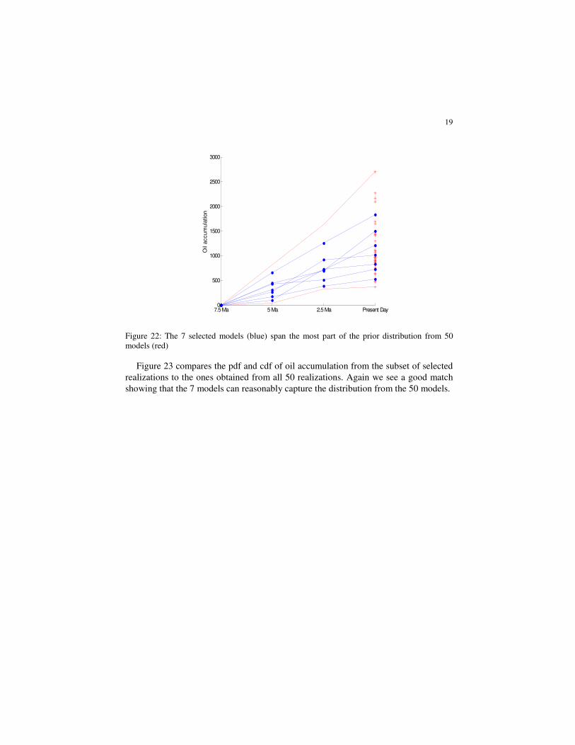
Is the subset of 7 realizations a good representative of the uncertainty space from

50 realizations? Figure 22 shows the oil accumulation for the 7 selected models (blue

dots) on top of all the 50 realizations (red stars). The accumulated oil volume through

time is plotted for each model. We see that the 7 selected realizations span most of the

original uncertainty space, though some extreme values are missed.

19

7.5 Ma 5 Ma 2.5 Ma Present Day0

500

1000

1500

2000

2500

3000

Oil

accum

ula

tion

Figure 22: The 7 selected models (blue) span the most part of the prior distribution from 50

models (red)

Figure 23 compares the pdf and cdf of oil accumulation from the subset of selected

realizations to the ones obtained from all 50 realizations. Again we see a good match

showing that the 7 models can reasonably capture the distribution from the 50 models.

20

0 500 1000 1500 2000 2500 30000

0.5

1

1.5x 10

-3

pdf from 50 models

pdf from 7 samples

0 500 1000 1500 2000 2500 30000

0.2

0.4

0.6

0.8

1

cdf from 50 models

cdf from 7 samples

Figure 23: Comparison of 7 models from kernel K-mean clustering to the 50 prior models shows

a good match for estimated pdf and cdf

6. Conclusions and future work

Uncertainty is an intrinsic complication in Basin and Petroleum System Modeling

because of the large spatial and temporal scale of the problem. The traditional

methodology is to do Monte Carlo simulations on the input parameters. This is done in

this study as the benchmark. The spatial uncertainties including facies and structure

are not studied before. We applied the geostatistical methods to generate multiple

realizations of facies and structure map. The corresponding uncertainty in oil

accumulation and oil distribution is assessed. We showed that facies distribution has a

great impact on the simulation results and different geological interpretation could

lead to very different results. In fact, variations in the volume of accumulated oil due

to lithologic facies variations are equally if not more important than variations in TOC,

21

HI, and basal heat flow. Thus it is important that the modeling process account for

both varying lithologies within a reservoir rock and the spatial correlation among

them. Structure uncertainty on the other hand does not have as great impact in this

example as we expected. One reason is that we only considered the uncertainty in

time-to-depth conversion assuming the seismic picks are perfect. One important future

work is to investigate different time horizon interpretations.

7. Acknowledgement

The authors would like to thank Ken Peters, Les Magoon, and Oliver Schenk for their

help. Special thanks to Petter Abrahamsen for providing the COHIBA software

package. We would also like to thank Schlumberger for the PetroMod license, and the

sponsors of the Stanford Basin and Petroleum System Modeling (BPSM) consortium

and Stanford Center for Reservoir Forecasting (SCRF) for their support.

22

Bibliography

[1] Allen P. A. and Allen J. R., Basin Analysis. Blackwell Publishing, second

edition, 2005.

[2] Abrahamsen, P., 1992. Bayesian Kriging for seismic depth conversion of a

multi-layer reservoir, Fourth International Geostatistical Congress. Troia,

Portugal September 13-18.

[3] Abrahamsen, P., 1996, Geostatistics for Seismic Depth Conversion. Report,

NR-note SAND/06/1996, 9 pages.

[4] Corradi A., D. Ponti, P. Ruffo, and G. Spadini, 2003, A methodology for

prospect evaluation by probabilistic basin modeling, in S. Düppenbecker and

R. Marzi, eds., Multidimensional basin modeling, AAPG/Datapages Discovery

Series No. 7, p. 283– 293.

[5] Hantschel, T., Kauerauf, A., 2009. Fundamentals of Basin Modeling.

Springer-Verlag, Heidelberg, 425 pp.

[6] Magoon, L. B., and Dow, W. G., 1994, The Petroleum System: From

Source to Trap, American Association of Petroleum Geologists Memoir 60,

Tulsa, Oklahoma, 655 p.

[7] Omre, H., Halvorsen, K. B., 1989. The Bayesian bridge between simple and

universal kriging. Math. Geol., 21(7):767-785.

[8] Peters, K. E., 2009, Getting Started in Basin and Petroleum System

Modeling. American Association of Petroleum Geologists (AAPG) CD-ROM

#16, AAPG Datapages.

[9] Scheidt C., Caers J., A new method for uncertainty quantification using

distances and kernel methods. Application to a deepwater turbidite reservoir.

SPE J, 14 (4): 680-692, SPEJ 118740-PA

[10] Strebelle, S., 2002, Conditional Simulation of Complex Geological

Structures Using Multiple-Point Statistics: Mathematical Geology, v. 34, no. 1,

p. 1-22.

[11] Thore, P., A. Shtuka, M. Lecour, T. Ait-Ettajer, and R. Cognot, 2002,

Structural uncertainties: Determination, management, and applications:

Geophysics, 67, 840–852.

23

[12] Wendebourg, J., 2003, Uncertainty of petroleum generation using methods

of experimental design and response surface modeling: Application to the

Gippsland Basin, Australia, in S. Düppenbecker and R. Marzi, eds.,

Multidimensional basin modeling, AAPG/Datapages Discovery Series No. 7,

p. 295– 307.

[13] Zwach, C., and D. Carruthers, 1998, Honouring uncertainties in the

modelling of migration volumes and trajectories (abs.): IFE Symposium on

Advances in Understanding and Modelling Hydrocarbon Migration, Oslo,

Norway, December 7–8, 1998.