Linköping University Electronic Press

Book Chapter

Anisotropy Estimation of Trabecular Bone in Gray-Scale: Comparison Between Cone Beam and Micro Computed

Tomography Data

Rodrigo Moreno, Magnus Borga, Eva Klintström, Torkel Brismar and Örjan Smedby

Part of: Developments in Medical Image Processing and Computational Vision, 2015, João Manuel R.S. Tavares and Renato Natal Jorge eds.

ISBN: 978-3-319-13406-2 (print), 978-3-319-13407-9 (online)

The final publication is available at Springer via 10.1007/978-3-319-13407-9_13

Series: Lecture Notes in Computational Vision and Biomechanics, 2212-9391, No. 19

Copyright: Springer Verlag http://www.springer.com/gp/

Available at: Linköping University Electronic Press http://urn.kb.se/resolve?urn=urn:nbn:se:liu:diva-117950

Anisotropy estimation of trabecular bone ingray-scale: comparison between cone beam andmicro computed tomography data

Rodrigo Moreno, Magnus Borga, Eva Klintstrom, Torkel Brismar and OrjanSmedby

Abstract Measurement of anisotropy of trabecular bone has clinical relevance inosteoporosis. In this study, anisotropy measurements of 15 trabecular bone biop-sies from the radius estimated by different fabric tensors on images acquiredthrough cone beam computed tomography (CBCT) and micro computed tomog-

Rodrigo MorenoDepartment of Radiology and Department of Medical and Health SciencesLinkoping University, Linkoping, SwedenCenter for Medical Image Science and Visualization (CMIV)Linkoping University, Linkoping, SwedenLinkoping University, Campus US, 581 85 Linkoping, Sweden,e-mail: rodrigo.moreno@liu.se

Magnus BorgaDepartment of Biomedical EngineeringLinkoping University, Linkoping, SwedenCenter for Medical Image Science and Visualization (CMIV)Linkoping University, Linkoping, Swedene-mail: magnus.borga@liu.se

Eva KlintstromDepartment of Radiology and Department of Medical and Health SciencesLinkoping University, Linkoping, SwedenCenter for Medical Image Science and Visualization (CMIV)Linkoping University, Linkoping, Swedene-mail: eva.klintstrom@lio.se

Torkel BrismarDepartment of Radiology,Karolinska University Hospital at Huddinge, Huddinge, Sweden,e-mail: torkel.brismar@gmail.com

Orjan SmedbyDepartment of Radiology and Department of Medical and Health SciencesLinkoping University, Linkoping, SwedenCenter for Medical Image Science and Visualization (CMIV)Linkoping University, Linkoping, Swedene-mail: orjan.smedby@liu.se

1

2 R. Moreno et al.

raphy (micro-CT) were compared. The results show that the generalized mean in-tercept length (MIL) tensor performs better than the global gray-scale structure ten-sor, especially when the von Mises-Fisher kernel is applied. Also, the generalizedMIL tensor yields consistent results between the two scanners. These results suggestthat this tensor is appropriate for estimating anisotropy in images acquired in vivothrough CBCT.

Key words: Fabric tensors, CBCT, micro-CT, generalized MIL tensor, GST, Tra-becular bone

1 Introduction

Fabric tensors aim at modeling through tensors both orientation and anisotropy oftrabecular bone. Many methods have been proposed for computing fabric tensorsfrom segmented images, including boundary-, volume-, texture-based and alterna-tive methods (cf. [19] for a complete review). However, due to large bias generatedby partial volume effects, these methods are usually not applicable to images ac-quired in vivo, where the resolution of the images is in the range of the trabecularthickness. Recently, different methods have been proposed to deal with this prob-lem. In general, these methods directly compute the fabric tensor on the gray-scaleimage, avoiding in that way the problematic segmentation step.

Different imaging modalities can be used to generate 3D images of trabecularbone in vivo, including different magnetic resonance imaging (MRI) protocols andcomputed tomography (CT) modalities. The main disadvantages of MRI are that itrequires long acquisition times that can easily lead to motion-related artifacts andthat the obtained resolution with this technique is worse compared to the one ob-tained through CT in vivo [8]. Regarding CT modalities, cone beam CT (CBCT)[16, 22] and high-resolution peripheral quantitative CT (HR-pQCT) [1, 5] are twopromising CT techniques for in vivo imaging. Although these techniques are notappropriate to all skeletal sites, their use is appealing since they can attain higherresolutions and lower doses than standard clinical CT scanners. CBCT has the extraadvantages with respect to HR-pQCT that it is available in most hospitals in thewestern world, since it is used in clinical practice in dentistry wards, and, on top ofthat, the scanning time is shorter (30s vs. 3min), so it is less prone to motion artifactsthan HR-pQCT.

As already mentioned, there are many methods available for computing tensorsdescribing anisotropy in gray-scale [19]. A strategy for choosing the most appro-priate method is to assess how similar the tensors computed from a modality for invivo imaging (e.g., CBCT) are with respect to the ones computed from the refer-ence imaging modality (micro-CT) for the same specimens. This was actually thestrategy that we follow in this chapter.

From the clinical point of view, it seems more relevant to track changes inanisotropy than in the orientation of trabecular bone under treatment, since osteo-

Anisotropy computed on CBCT and micro-CT images 3

porosis can have more effect on its anisotropy than on its orientation [23, 13]. Thus,the aim of the present study was to compare anisotropy measurements from differentfabric tensors computed on images acquired through cone beam computed tomog-raphy (CBCT) to the same tensors computed on images acquired through microcomputed tomography (micro-CT).

Due to its flexibility, we have chosen in this study our previously proposed gen-eralized mean intercept length (MIL) tensor [17] (GMIL) with different kernels and,due to its simplicity, the global gray-scale structure tensor (GST) [26]. This chapteris an extended version of the work in [18].

The chapter is organized as follows. Section 2 presents the material and methodsused in this study. Section 3 shows comparisons between using GMIL and GST inboth CBCT and micro-CT data. Finally, Sect. 4 discusses the results and outlinesour current ongoing research.

2 Material and methods

2.1 Material

The samples in this study consisted of 15 bone biopsies from the radius of humancadavers donated to medical research. The biopsies were approximately cubic with aside of 10 mm. Each cube included a portion of cortical bone on one side to facilitateorientation. The bone samples were placed in a test tube filled with water and thetube was placed in the centre of a paraffin cylinder, with a diameter of approximately10 cm, representing soft tissue to simulate measurements in vivo. After imaging, acube, approximately 8 mm in side, with only trabecular bone was digitally extractedfrom each dataset for analysis.

2.2 Image acquisition and reconstruction

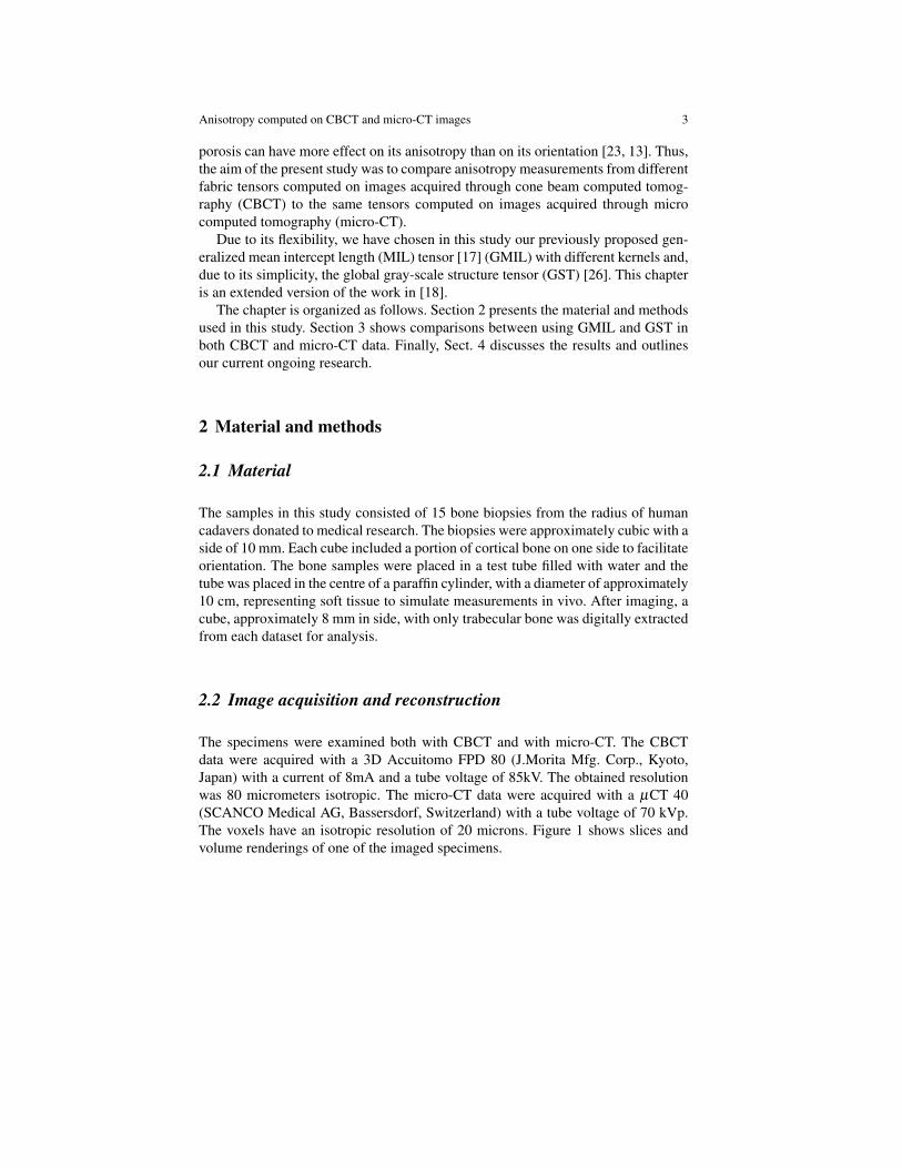
The specimens were examined both with CBCT and with micro-CT. The CBCTdata were acquired with a 3D Accuitomo FPD 80 (J.Morita Mfg. Corp., Kyoto,Japan) with a current of 8mA and a tube voltage of 85kV. The obtained resolutionwas 80 micrometers isotropic. The micro-CT data were acquired with a µCT 40(SCANCO Medical AG, Bassersdorf, Switzerland) with a tube voltage of 70 kVp.The voxels have an isotropic resolution of 20 microns. Figure 1 shows slices andvolume renderings of one of the imaged specimens.

4 R. Moreno et al.

(a) (b)

(c) (d)

Fig. 1 Slices (left) and volume renderings (right) of one of the imaged specimens. Top: imagesacquired through micro-CT. Bottom: images acquired through CBCT.

2.3 Methods

The tensors were computed through the generalized MIL tensor (GMIL) and theGST.

2.3.1 GMIL tensor

Basically, the GMIL tensor is computed in three steps. The mirrored extended Gaus-sian image (EGI) [12] is computed from a robust estimation of the gradient. Second,the EGI is convolved with a kernel in order to obtain an orientation distribution func-tion (ODF). Finally, a second-order fabric tensor is computed from the ODF. Moreformally, the generalized MIL tensor is computed as:

MIL=∫

Ω

vvT

C(v)2 dΩ , (1)

where v are vectors on the unitary sphere Ω , and C is given by:

C = H ∗E, (2)

Anisotropy computed on CBCT and micro-CT images 5

that is, the angular convolution (∗) of a kernel H with the mirrored EGI E. Thanks tothe Funk-Hecke theorem [9, 3], this convolution can be performed efficiently in thespherical harmonics domain when the kernel is positive and rotationally symmetricwith respect to the north pole.

One of the advantages of the GMIL tensor is that different kernels can be usedin order to improve the results. In this study, the half-cosine (HC) and von Mises-Fisher (vMF) kernels have been applied to the images. The HC has been selectedsince it makes equivalent the generalized and the original MIL tensor. The HC isgiven by:

H(φ) =

cos(φ) ,if φ ≤ π/20 ,otherwise, (3)

with φ being the polar angle in spherical coordinates. Moreover, the vMF kernel,which is given by [14]:

H(φ) =κ

4π sinh(κ)eκ cos(φ), (4)

has been selected since it has a parameter κ that can be used to control its smoothingaction. In particular, the smoothing effect is reduced as the values of κ are increased[17].

Figure 2 shows different kernels that can be used with the GMIL tensor. As al-ready mentioned, these kernels must be positive and symmetric with respect to thenorth pole. As shown in the figure, the HC kernel is too broad (it covers half ofthe sphere), which can result in excessive smoothing. On the contrary, the impulsekernel is the sharpest possible kernel. As shown in [17], the GST makes use of theimpulse kernel. In turn, the size of the smoothing effect of the vMF kernel can becontrolled through the parameter κ . As shown in the figure, vMF is broader than theHC for small values of κ and it converges to the impulse kernel in the limit whenκ → ∞.

2.3.2 GST tensor

On the other hand, the GST computes the fabric tensor by adding up the outer prod-uct of the local gradients with themselves [26], that is:

GST=∫

p∈I∇Ip ∇IT

p dI, (5)

where I is the image and ∇Ip is the gradient.Notice that GST related to the well-known local structure tensor (ST) which has

been used in the computer vision community since 1980s [4]. There are differentmethods for computing ST, including quadrature filters [7], higher-order derivatives[15] or tensor voting [20]. However, the most used ST is given by:

STσ (p) = Gσ ∗∇Ip∇IpT (6)

6 R. Moreno et al.

vMF (κ = 1) HC vMF (κ = 5)

vMF (κ = 10) vMF (κ = 50) Impulse

Fig. 2 Graphical representation of some kernels from the broadest to the narrowest, where zeroand the largest values are depicted in blue and red respectively. Notice that the impulse kernel hasbeen depicted as a single red dot in the north pole of the sphere.

where Gσ is a Gaussian weighting function with zero mean and standard deviationσ . In fact, ST becomes the GST when σ →∞. The main advantage of this structuretensor is that it is easy to code.

3 Results

As already mentioned, the focus in this chapter is the estimation of anisotropy. As amatter of fact, both the GMIL (and therefore the MIL tensor) and the GST tensorsyield the same orientation information, since they have the same eigenvectors (cf.[17] for a detailed proof). This means that only the eigenvalues of the tensors are ofinterest for the purposes of this chapter.

The following three values have been computed for each tensor:

E1′ = E1/(E1+E2+E3)E2′ = E2/E1,E3′ = E3/E1,

where E1, E2 and E3 are the largest, intermediate and smallest eigenvalues of thetensor. These three values have been selected since they are directly related to theshape of the tensor.

Anisotropy computed on CBCT and micro-CT images 7

Table 1 Mean (SD) of E1’ for fabric tensors computed on CBCT and micro-CT and the meandifference (SD) between both values. HC and vMF refer to the generalized MIL tensor, with theHC, and vMF kernels respectively. Parameter κ for vMF is shown in parenthesis. Positive andnegative values of the difference mean over- and under estimations of CBCT with respect to micro-CT. All values have been multiplied by 100.

Tensor micro-CT CBCT DifferenceHC 44.65 (1.54) 42.38 (0.90) 2.25 (0.84)vMF(1) 34.12 (0.29) 34.70 (0.18) 0.42 (0.15)vMF(5) 51.55 (3.56) 47.07 (2.17) 4.51 (1.82)vMF(10) 58.98 (4.63) 53.90 (3.21) 5.11 (2.13)GST 45.69 (1.58) 44.79 (1.58) 0.90 (2.09)

Table 2 Mean (SD) of E2’ for fabric tensors computed on CBCT and micro-CT and the meandifference (SD) between both values. HC and vMF refer to the generalized MIL tensor, with theHC, and vMF kernels respectively. Parameter κ for vMF is shown in parenthesis. Positive andnegative values of the difference mean over- and under estimations of CBCT with respect to micro-CT. All values have been multiplied by 100.

Tensor micro-CT CBCT DifferenceHC 65.94 (5.85) 71.50 (3.53) -6.11 (2.19)vMF(1) 93.70 (1.69) 95.27 (1.02) -1.84 (0.73)vMF(5) 52.13 (9.54) 61.63 (6.53) -8.48 (3.09)vMF(10) 39.41 (9.74) 48.31 (7.75) -8.96 (4.43)GST 80.71 (10.66) 78.58 (7.66) 2.24 (7.41)

Table 3 Mean (SD) of E3’ for fabric tensors computed on CBCT and micro-CT and the meandifference (SD) between both values. HC and vMF refer to the generalized MIL tensor, with theHC, and vMF kernels respectively. Parameter κ for vMF is shown in parenthesis. Positive andnegative values of the difference mean over- and under estimations of CBCT with respect to micro-CT. All values have been multiplied by 100.

Tensor micro-CT CBCT DifferenceHC 58.29 (2.93) 65.18 (2.20) -5.58 (2.98)vMF(1) 91.09 (1.01) 92.92 (0.67) -1.59 (0.89)vMF(5) 42.72 (5.11) 51.20 (3.71) -9.55 (4.49)vMF(10) 31.17 (4.94) 37.81 (3.91) -6.64 (2.70)GST 38.71 (4.90) 44.96 (3.78) -6.31 (4.40)

Tables 1-3 show the mean and standard deviation of E1’, E2’ and E3’ computedon micro-CT and CBCT for the tested methods, and the mean difference and stan-dard deviation between micro-CT and CBCT. As a general trend, the tested methodstend to overestimate E1’ and underestimate E2’ and E3’ in CBCT. As shown, thebest performance is obtained by vMF with κ =1 with small differences between ten-sors computed in both modalities. However, the tensors computed with this broadkernel are almost isotropic (cf. Tables 2 and 3), which makes it not suitable fordetecting anisotropies in trabecular bone. It is also worthwhile to notice that thestandard deviation of the differences increases with narrower kernels, such as GST.This means that a mild smoothing effect from middle range kernels such as vMFwith κ=10, have a positive effect in the estimation of fabric tensors, since the dif-

8 R. Moreno et al.

ferences between micro-CT and CBCT are reduced while keeping the anisotropy ofthe tensors.

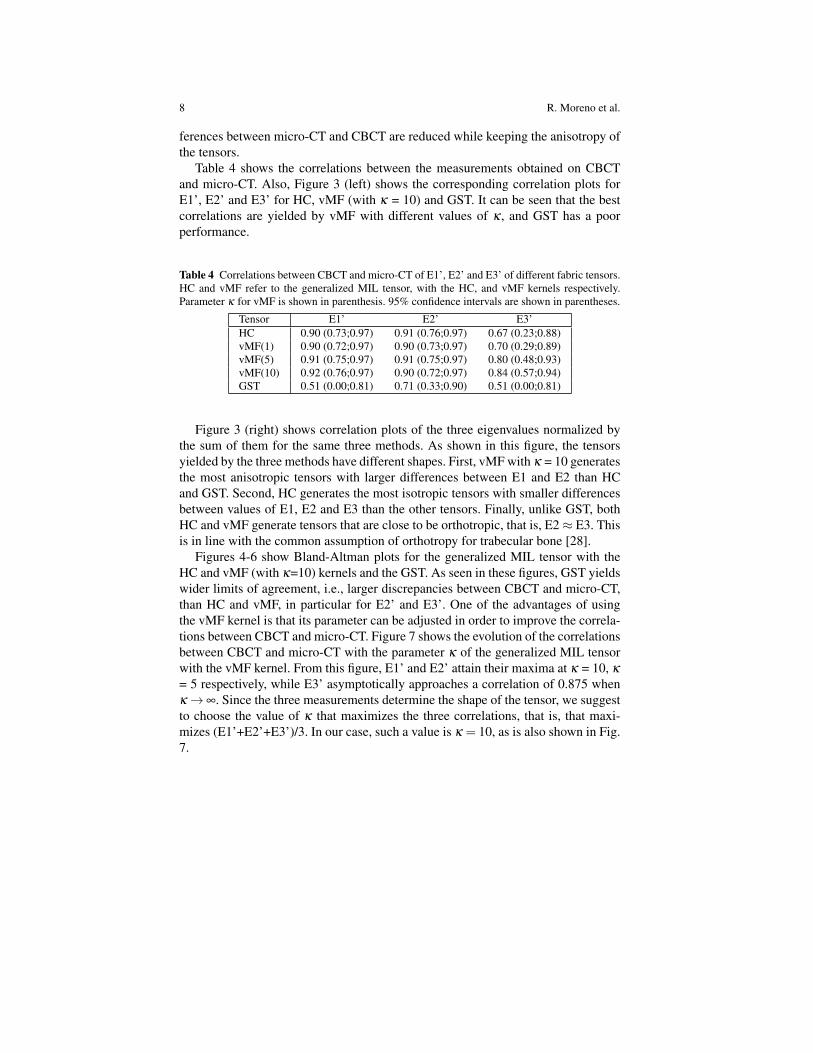
Table 4 shows the correlations between the measurements obtained on CBCTand micro-CT. Also, Figure 3 (left) shows the corresponding correlation plots forE1’, E2’ and E3’ for HC, vMF (with κ = 10) and GST. It can be seen that the bestcorrelations are yielded by vMF with different values of κ , and GST has a poorperformance.

Table 4 Correlations between CBCT and micro-CT of E1’, E2’ and E3’ of different fabric tensors.HC and vMF refer to the generalized MIL tensor, with the HC, and vMF kernels respectively.Parameter κ for vMF is shown in parenthesis. 95% confidence intervals are shown in parentheses.

Tensor E1’ E2’ E3’HC 0.90 (0.73;0.97) 0.91 (0.76;0.97) 0.67 (0.23;0.88)vMF(1) 0.90 (0.72;0.97) 0.90 (0.73;0.97) 0.70 (0.29;0.89)vMF(5) 0.91 (0.75;0.97) 0.91 (0.75;0.97) 0.80 (0.48;0.93)vMF(10) 0.92 (0.76;0.97) 0.90 (0.72;0.97) 0.84 (0.57;0.94)GST 0.51 (0.00;0.81) 0.71 (0.33;0.90) 0.51 (0.00;0.81)

Figure 3 (right) shows correlation plots of the three eigenvalues normalized bythe sum of them for the same three methods. As shown in this figure, the tensorsyielded by the three methods have different shapes. First, vMF with κ = 10 generatesthe most anisotropic tensors with larger differences between E1 and E2 than HCand GST. Second, HC generates the most isotropic tensors with smaller differencesbetween values of E1, E2 and E3 than the other tensors. Finally, unlike GST, bothHC and vMF generate tensors that are close to be orthotropic, that is, E2≈ E3. Thisis in line with the common assumption of orthotropy for trabecular bone [28].

Figures 4-6 show Bland-Altman plots for the generalized MIL tensor with theHC and vMF (with κ=10) kernels and the GST. As seen in these figures, GST yieldswider limits of agreement, i.e., larger discrepancies between CBCT and micro-CT,than HC and vMF, in particular for E2’ and E3’. One of the advantages of usingthe vMF kernel is that its parameter can be adjusted in order to improve the correla-tions between CBCT and micro-CT. Figure 7 shows the evolution of the correlationsbetween CBCT and micro-CT with the parameter κ of the generalized MIL tensorwith the vMF kernel. From this figure, E1’ and E2’ attain their maxima at κ = 10, κ

= 5 respectively, while E3’ asymptotically approaches a correlation of 0.875 whenκ→∞. Since the three measurements determine the shape of the tensor, we suggestto choose the value of κ that maximizes the three correlations, that is, that maxi-mizes (E1’+E2’+E3’)/3. In our case, such a value is κ = 10, as is also shown in Fig.7.

Anisotropy computed on CBCT and micro-CT images 9

R² = 0.8188

R² = 0.8379

R² = 0.2649

0.40

0.50

0.60

0.70

0.40 0.50 0.60 0.70

CBCT

micro-CT

HC vMF(10) GST

R² = 0.8364

R² = 0.8101

R² = 0.517

0.20

0.40

0.60

0.80

1.00

0.20 0.40 0.60 0.80 1.00

CBCT

micro-CT

HC vMF(10) GST

R² = 0.4426

R² = 0.7031

R² = 0.2608

0.20

0.30

0.40

0.50

0.60

0.70

0.20 0.30 0.40 0.50 0.60 0.70

CBCT

micro-CT

HC vMF(10) GST

R² = 0.8188R² = 0.7698

R² = 0.2262

0.10

0.20

0.30

0.40

0.50

0.60

0.70

0.10 0.30 0.50 0.70

CBCT

micro-CT

E1 E2 E3

R² = 0.8379

R² = 0.7974

R² = 0.466

0.10

0.20

0.30

0.40

0.50

0.60

0.70

0.10 0.30 0.50 0.70

CBCT

micro-CT

E1 E2 E3

R² = 0.2649

R² = 0.6614

R² = 0.5416

0.10

0.20

0.30

0.40

0.50

0.60

0.70

0.10 0.30 0.50 0.70

CBCT

micro-CT

E1 E2 E3

Fig. 3 Left: correlation plots for E1’ (top), E2’ (middle) and E3’ (bottom) between CBCT andmicro-CT for HC, vMF (κ = 10) and GST. Right: correlation plots for HC (top), vMF (κ=10)(middle) and GST (bottom) between CBCT and micro-CT for the three eigenvalues normalized bythe sum of them.

10 R. Moreno et al.

0.00

0.01

0.02

0.03

0.04

0.41 0.42 0.43 0.44 0.45 0.46 0.47

-0.12

-0.09

-0.06

-0.03

0

0.55 0.60 0.65 0.70 0.75 0.80

-0.12

-0.1

-0.08

-0.06

-0.04

-0.02

0

0.56 0.58 0.60 0.62 0.64 0.66 0.68

Fig. 4 Bland-Altman plots for E1’ (top), E2’ (middle) and E3’ (bottom) between CBCT and micro-CT for HC. The vertical and horizontal axes show the measurements on micro-CT minus thosecomputed on CBCT, and the mean between them respectively. The mean difference and the meandifference ± 1.96 SD are included as a reference in dotted lines.

4 Discussion

We have compared in this chapter the anisotropy of different fabric tensors estimatedon images acquired through CBCT and micro-CT of 15 trabecular bone biopsiesfrom the radius. The results presented in the previous section show strong correla-tions between micro-CT and CBCT for the generalized MIL tensor with HC andvMF kernels, especially with κ = 10. In addition, good agreements between mea-surements in CBCT and the reference micro-CT have been shown through Bland-Altman plots for HC, vMF with κ = 10 and GST. An interesting result is that theGST yields clearly lower correlation values than the generalized MIL tensor usingeither HC or vMF kernels. We have shown that the GST can be seen as a variant ofthe generalized MIL tensor where the impulse kernel is applied instead of the HC[17].

In this line, the results from the previous section suggest that the use of broadersmoothing kernels such as HC or vMF has a positive effect for increasing the corre-

Anisotropy computed on CBCT and micro-CT images 11

0.00

0.02

0.04

0.06

0.08

0.10

0.45 0.55 0.65

-0.18

-0.14

-0.1

-0.06

-0.02

0.25 0.35 0.45 0.55 0.65

-0.15

-0.12

-0.09

-0.06

-0.03

0

0.30 0.35 0.40 0.45

Fig. 5 Bland-Altman plots for E1’ (top), E2’ (middle) and E3’ (bottom) between CBCT and micro-CT for vMF with κ=10. The vertical and horizontal axes show the measurements on micro-CTminus those computed on CBCT, and the mean between them respectively. The mean differenceand the mean difference ± 1.96 SD are included as a reference in dotted lines.

lation of the tensors computed on images acquired through suitable scanners for invivo with the ones that can be computed from images acquired in vitro. Althoughthe three tested methods yield tensors that share their eigenvectors, their eigenval-ues are different, as shown in Figure 3, which is a natural consequence of usingdifferent smoothing kernels. Moreover, the high correlations reported for HC andvMF enable to eliminate of the systematic errors reported in Tables 1-3 and in theBland-Altman plots for these two types of fabric tensors.

Another interesting observation is that vMF yielded better results than the stan-dard HC. This means that κ can be used to tune the smoothing in such a way thatthe results are correlated with in vitro measurements. For the imaged specimens, avalue of κ = 10 yielded the best correlation results.

The results presented in this chapter suggest that advanced fabric tensors aresuitable for in vivo imaging, which opens the door to their use in clinical practice.In particular, the results show that the generalized MIL tensor is the most promisingoption for use in vivo. As shown in this chapter, this method is advantageous since

12 R. Moreno et al.

-0.04

-0.02

0.00

0.02

0.04

0.40 0.42 0.44 0.46 0.48 0.50

-0.13

-0.08

-0.03

0.02

0.07

0.12

0.17

0.60 0.70 0.80 0.90

-0.15

-0.12

-0.09

-0.06

-0.03

0

0.03

0.30 0.35 0.40 0.45 0.50

Fig. 6 Bland-Altman plots for E1’ (top), E2’ (middle) and E3’ (bottom) between CBCT and micro-CT for GST. The vertical and horizontal axes show the measurements on micro-CT minus thosecomputed on CBCT, and the mean between them respectively. The mean difference and the meandifference ± 1.96 SD are included as a reference in dotted lines.

0.68

0.73

0.78

0.83

0.88

0.93

5 10 15 20 25 30 35 40 45 50

Correlation

κκκκ

E1'

E2'

E3'

(E1'+E2'+E3')/3

Fig. 7 Evolution of the correlations between CBCT and micro-CT with the parameter κ of thegeneralized MIL tensor with the vMF kernel.

Anisotropy computed on CBCT and micro-CT images 13

it has the possibility to improve its performance by changing the smoothing kernelby a more appropriate one, as it was shown in this chapter for the vMF kernel.

A poor performance of the GST has also been reported in images acquiredthrough multi-slice computed tomography (MSCT) [25]. The authors of that studyhypothesized that such a bad performance could be due to voxel anisotropy obtainedfrom MSCT. However, the results from the current study suggest that the problemsof the GST are more structural, since they are also present in CBCT with isotropicvoxels. Thus, the problems of GST seem more related to the applied kernel (theimpulse kernel) than to the voxel anisotropy of the images.

Ongoing research includes performing comparisons in different skeletal sites,different degrees of osteoporosis and comparing the results with images acquiredthrough HR-pQCT and micro-MRI [11, 6]. Furthermore, relationships between fab-ric and elasticity tensors will be explored. The MIL tensor has extensively been usedfor predicting elasticity tensors in trabecular bone [2, 27, 10]. However, since theGMIL with the vMF kernel has a better performance than the MIL tensor for re-producing in vitro measurements, we want to investigate whether or not the GMILtensor can also be used to increase the accuracy of the MIL tensor for predicting theelastic properties of trabecular bone.

In the same line, we have recently hypothesized that trabecular termini (i.e., freeended trabeculae [24]) should not be considered for computing fabric tensors sincecontribution of termini to the mechanical competence of trabecular bone is ratherlimited [21]. Thus, it is worthwhile to assess the power of fabric tensors that disre-gard termini for predicting elasticity.

Acknowledgements We thank Andres Laib from SCANCO Medical AG for providing the micro-CT data of the specimens. The authors declare no conflict of interest.

References

1. Burghardt, A., Link, T., Majumdar, S.: High-resolution computed tomography for clinicalimaging of bone microarchitecture. Clinical Orthopaedics and Related Research 469(8),2179–2193 (2011)

2. Cowin, S.: The relationship between the elasticity tensor and the fabric tensor. Mechachics ofMaterials 4(2), 137–147 (1985)

3. Driscoll, J.R., Healy, D.M.: Computing Fourier transforms and convolutions on the 2-sphere.Advances in Applied Mathematics 15(2), 202–250 (1994)

4. Forstner, W.: A feature based correspondence algorithm for image matching. In: The Interna-tional Archives of the Photogrammetry and Remote Sensing, vol. 26, pp. 150–166 (1986)

5. Geusens, P., Chapurlat, R., Schett, G., Ghasem-Zadeh, A., Seeman, E., de Jong, J., van denBergh, J.: High-resolution in vivo imaging of bone and joints: a window to microarchitecture.Nature Reviews Rheumatology (2014). In press

6. Gomberg, B., Wehrli, F., Vasili’c, B., Weening, R., Saha, P., Song, H., Wright, A.: Repro-ducibility and error sources of -mri-based trabecular bone structural parameters of the distalradius and tibia. Bone 35(1), 266 – 276 (2004)

7. Granlund, G.H., Knutsson, H.: Signal Processing for Computer Vision. Kluwer AcademicPublishers, Dordrecht The Netherlands (1995)

14 R. Moreno et al.

8. Griffith, J., Genant, H.: New advances in imaging osteoporosis and its complications. En-docrine 42, 39–51 (2012)

9. Groemer, H.: Geometric applications of Fourier series and spherical harmonics. CambridgeUniversity Press (1996)

10. Gross, T., Pahr, D., Zysset, P.: Morphology-elasticity relationships using decreasing fabricinformation of human trabecular bone from three major anatomical locations. Biomechanicsand Modeling in Mechanobiology 12(4), 793–800 (2013)

11. Hipp, J., Jansujwicz, A., Simmons, C., Snyder, B.: Trabecular bone morphology from micro-magnetic resonance imaging. Journal of Bone Mineral Research 11(2), 286–297 (1996)

12. Horn, B.K.P.: Extended Gaussian images. Proceedings of the IEEE 72(12), 1671–1686 (1984)13. Huiskes, R.: If bone is the answer, then what is the question? Journal of Anatomy 197, 145–

156 (2000)14. Jupp, P.E., Mardia, K.V.: A unified view of the theory of directional statistics, 1975-1988.

International Statistics Review 57(3), 261–294 (1989)15. Kothe, U., Felsberg, M.: Riesz-transforms versus derivatives: On the relationship between the

boundary tensor and the energy tensor. In: Scale Space and PDE Methods in Computer Vision,Hofgeismar Germany, LNCS, vol. 3459, pp. 179–191 (2005)

16. Monje, A., Monje, F., Gonzalez-Garcia, R., Galindo-Moreno, P., Rodriguez-Salvanes, F.,Wang, H.: Comparison between microcomputed tomography and cone-beam computed to-mography radiologic bone to assess atrophic posterior maxilla density and microarchitecture.Clinical Oral Implants Research pp. 1–6 (2013)

17. Moreno, R., Borga, M., Smedby, O.: Generalizing the mean intercept length tensor for gray-level images. Medical Physics 39(7), 4599–4612 (2012)

18. Moreno, R., Borga, M., Smedby, O.: Correlations between fabric tensors computed on conebeam and micro computed tomography images. In: J. Tavares, R. Natal-Jorge (eds.) Compu-tational Vision and Medical Image Processing (VIPIMAGE), pp. 393–398. CRC Press (2013)

19. Moreno, R., Borga, M., Smedby, O.: Techniques for computing fabric tensors: a review. In:B. Burgeth, A. Vilanova, C.F. Westin (eds.) Visualization and Processing of Tensors andHigher Order Descriptors for Multi-Valued Data. Springer (2014). In press

20. Moreno, R., Pizarro, L., Burgeth, B., Weickert, J., Garcia, M.A., Puig, D.: Adaptation of tensorvoting to image structure estimation. In: D. Laidlaw, A. Vilanova (eds.) New Developmentsin the Visualization and Processing of Tensor Fields, pp. 29–50. Springer (2012)

21. Moreno, R., Smedby, O.: Volume-based fabric tensors through lattice-Boltzmann simulations.In: Proceedings International Conference on Pattern Recognition (ICPR), Stockholm Sweden(2014). Accepted

22. Mulder, L., van Rietbergen, B., Noordhoek, N.J., Ito, K.: Determination of vertebral andfemoral trabecular morphology and stiffness using a flat-panel C-arm-based CT approach.Bone 50(1), 200–208 (2012)

23. Odgaard, A., Kabel, J., van Rietbergen, B., Dalstra, M., Huiskes, R.: Fabric and elastic princi-pal directions of cancellous bone are closely related. Journal of Biomechanics 30(5), 487–495(1997)

24. Tabor, Z.: Novel algorithm detecting trabecular termini in µCT and MRI images. Bone 37(3),395–403 (2005)

25. Tabor, Z., Petryniak, R., Latała, Z., Konopka, T.: The potential of multi-slice computed tomog-raphy based quantification of the structural anisotropy of vertebral trabecular bone. MedicalEngineering & Physics 35(1), 7 – 15 (2013)

26. Tabor, Z., Rokita, E.: Quantifying anisotropy of trabecular bone from gray-level images. Bone40(4), 966–972 (2007)

27. Zysset, P.K.: A review of morphology-elasticity relationships in human trabecular bone: the-ories and experiments. Journal of Biomechanics 36(10), 1469–1485 (2003)

28. Zysset, P.K., Goulet, R.W., Hollister, S.J.: A global relationship between trabecular bone mor-phology and homogenized elastic properties. Journal of Biomechanical Engineering 120(5),640–646 (1998)