New Nonparametric Tests of Multivariate Locations and Scales Using Data DepthAuthor(s): Jun Li and Regina Y. LiuReviewed work(s):Source: Statistical Science, Vol. 19, No. 4 (Nov., 2004), pp. 686-696Published by: Institute of Mathematical StatisticsStable URL: http://www.jstor.org/stable/4144439 .Accessed: 11/10/2012 19:07

Your use of the JSTOR archive indicates your acceptance of the Terms & Conditions of Use, available at .http://www.jstor.org/page/info/about/policies/terms.jsp

.JSTOR is a not-for-profit service that helps scholars, researchers, and students discover, use, and build upon a wide range ofcontent in a trusted digital archive. We use information technology and tools to increase productivity and facilitate new formsof scholarship. For more information about JSTOR, please contact support@jstor.org.

.

Institute of Mathematical Statistics is collaborating with JSTOR to digitize, preserve and extend access toStatistical Science.

http://www.jstor.org

Statistical Science 2004, Vol. 19, No. 4, 686-696 DOI 10.1214/088342304000000594 ? Institute of Mathematical Statistics, 2004

New Nonparametric Tests of Multivariate

Locations and Scales Using Data Depth Jun Li and Regina Y. Liu

Abstract. Multivariate statistics plays a role of ever increasing importance in the modem era of information technology. Using the center-outward rank- ing induced by the notion of data depth, we describe several nonparametric tests of location and scale differences for multivariate distributions. The tests for location differences are derived from graphs in the so-called DD plots (depth vs. depth plots) and are implemented through the idea of permutation tests. The proposed test statistics are scale-standardized measures for the lo- cation difference and they can be carried out without estimating the scale or variance of the underlying distributions. The test for scale differences intro- duced in Liu and Singh (2003) is a natural multivariate rank test derived from the center-outward depth ranking and it extends the Wilcoxon rank-sum test to the testing of multivariate scale. We discuss the properties of these tests, and provide simulation results as well as a comparison study under normality. Finally, we apply the tests to compare airlines' performances in the context of aviation safety evaluations.

Key words and phrases: Data depth, DD plot, multivariate location differ- ence, multivariate scale difference, permutation test, multivariate rank test, Wilcoxon rank-sum test.

1. INTRODUCTION

Recent advances in computer technology have fa- cilitated the collection of massive multivariate data in many industries. The demand for effective multivariate analyses has never been greater. Most existing multi- variate analysis still relies on the assumption of nor- mality, which is often difficult to justify in practice. Using the center-outward ranking induced by the no- tion of data depth, we describe several nonparametric tests for location and scale differences in multivariate distributions. These tests are completely nonparametric and have broader applicability than the existing tests. They can even be moment-free and thus valid for test- ing parameters which are not defined using moments, such as the locations of Cauchy distributions.

For testing location differences, our test statistics are constructed from the graphs observed in the DD plots

(depth vs. depth plots). The DD plot, introduced by Liu, Parelius and Singh (1999), is a two-dimensional graph which can serve as a simple diagnostic tool for visual comparisons of two samples of any dimension. Different distributional differences, such as location, scale, skewness or kurtosis differences, are associated with different graphical patterns in DD plots. In this paper, we focus on the pattern associated with the lo- cation difference in the DD plots and we propose two tests for testing possible location differences between two samples. Since the data depth is affine-invariant, it provides a scale-standardized measure of the po- sition of any data point relative to the center of the distribution. This property allows us to view our depth- based test statistics as scale-standardized measures for the location difference. Consequently, the tests can be carried out without the difficulty of estimating the variance of the null sampling distributions. Instead, we derive the decision rules by obtaining p-values using the idea of permutation.

For testing multivariate scales, we review a new rank test proposed by Liu and Singh (2003). This rank

Jun Li is a Ph.D. candidate and Regina Y Liu is Pro- fessor Department of Statistics, Rutgers University, Piscataway, New Jersey 08854-8019, USA (e-mail: junli@stat.rutgers.edu, rliu@stat.rutgers.edu).

686

TESTS OF MULTIVARIATE LOCATIONS AND SCALES 687

test is derived from the center-outward ranking in- duced by data depth assigned to the combined sam- ple. It is constructed in a way similar to the Wilcoxon rank-sum test and can be carried out using either the Wilcoxon rank-sum table or simulations. It is a com- pletely nonparametric test for testing the scale expan- sion or contraction. It includes the Ansari-Bradley and the Siegel-Tukey tests as special cases for testing the equality of variances in the univariate setting.

The tests discussed in this paper are appealing since they are guided visually by the DD plot and admit a full theoretical justification. Most importantly, they are easy to implement regardless of the dimensionality of the data. For all the proposed tests, we present several simulation studies, including power comparisons be- tween our proposed nonparametric tests and some ex- isting parametric tests. The performance of our tests is generally comparable to the parametric tests under the multivariate normal setting, with only minor loss of efficiency. However, our tests dramatically outperform the parametric tests under the multivariate Cauchy set- ting. This is in part because our tests are moment-free and thus are more suitable for dealing with parameters not derived from moments, such as those in the case of Cauchy distributions.

The rest of the paper is organized as follows. In Sec- tion 2 we give a brief review of the notion of data depth, depth-induced multivariate rankings and DD plots. In Section 3 we describe two tests for location differ- ences. These tests are referred to as the T-based test and the M-based test, and they are derived from the graphs in DD plots which reflect location changes be- tween two distributions. We then carry out the tests by using Fisher's permutation test to determine p-values. We justify the validity of the tests by showing that the distribution of the obtained p-values follows ap- proximately the uniform distribution U[0, 1] under the null hypothesis and also that it decreases to 0 under the alternative hypothesis. Results from several simu- lation studies are presented. Under the normality as- sumption, our tests are comparable to the Hotelling T2 test. We devote Section 4 to the scale comparison of two multivariate distributions, which includes a depth- induced multivariate rank test introduced in Liu and Singh (2003) and a graphical display of scale curve (Liu, Parelius and Singh, 1999). In Section 5 we ap- ply our tests to compare the performance of 10 air- lines using the airline performance data collected by the Federal Aviation Administration (FAA). Finally, we provide some concluding remarks in Section 6.

2. NOTATION AND BACKGROUND MATERIAL

We begin with a brief description of the notion of data depth and its properties.

2.1 Data Depth and Center-Outward Ranking of Multivariate Data

A data depth is a way to measure the "depth" or

"outlyingness" of a given point with respect to a mul- tivariate data cloud or its underlying distribution. It gives rise to a natural center-outward ordering of the

sample points in a multivariate sample. This ordering gives rise to new and easy ways to quantify the many complex multivariate features of the underlying distri- bution, including location, quantiles, scale, skewness and kurtosis. This ordering in effect turn provides a new nonparametric multivariate inference scheme (cf. Liu, Parelius and Singh, 1999), which includes sev- eral graphical methods for comparing multivariate dis- tributions or samples. Some of the methods in Liu, Parelius and Singh (1999) motivated the comparison methods presented in this paper. Before we show how the depth and its ordering can be used to construct mul- tivariate nonparametric tests, we first use the simpli- cial depth proposed by Liu (1990) as an example of depth measure (1) to describe the general concept of data depth and its corresponding center-outward order- ing, and (2) to introduce necessary notation.

The word "depth" was first used by Tukey (1975) to picture data, and the far reaching ramifications of

depth in ordering and analyzing multivariate data was observed and elaborated by Liu (1990), Donoho and Gasko (1992), Liu, Parelius and Singh (1999) and oth- ers. Many existing notions of data depth were listed in Liu, Parelius and Singh (1999).

Let { Y1,..., Y,, } be a random sample from the dis- tribution G(.) in IRk, k > 1. We begin with the bivari- ate setting k = 2. Let A(a, b, c) denote a triangle with vertices a, b and c. Let I(.) be the indicator function, that is, I(A) = 1 if A occurs and I (A) = 0 otherwise. Given the sample {Y1,..., Y, }, the sample simplicial depth of y e R2 is defined as

-1 (2.1) DGm(Y) =() I(y A(Yil, Yi2, Yi3)) (*)

which is the fraction of the triangles generated from the sample that contain the point y. Here (*) runs over all possible triplets of { Y1,..., Y,m }. A large value of DGm (Y) indicates that y is contained in many tri- angles generated from the sample, and thus it lies

deep within the data cloud. On the other hand, a small

688 J. LI AND R. Y. LIU

DGm (y) indicates an outlying position of y. Thus DGm is a measure of the depth (or outlyingness) of y w.r.t. the data cloud { Yi,..., Ym).

The above simplicial depth can be generalized to any dimension k as

DGm(Y) (2.2)

Skm+ 1 I (y E

s[Yil

,

I(Yik+1), (,;,)l~l(*)[?;y~1

where (*) runs over all possible subsets of { Y1,..., Ym } of size k + 1. Here s[Yi, ..., Yik+l] is the closed sim- plex whose vertices are {Yil,..., Yik+1}, that is, the smallest convex set determined by {Yi1,., ..Yik+1 }. When the distribution G is known, then the simplicial depth of y w.r.t. to G is defined as

(2.3) DG(y) = PGY E s[Y1, ... , Yk+l]}, where Y1,..., Yk+l are k + 1 random observations from G. Depth DG(y) measures how deep y is w.r.t. G. A fuller motivation together with the basic properties of DG(.) can be found in Liu (1990). In particular, it is shown that DG (.) is affine-invariant and that DGm (') converges uniformly and strongly to DG(.). The affine invariance ensures that our proposed inference meth- ods are coordinate-free, and the convergence of DGm to DG allows us to approximate DG(.) by DGm () when G is unknown.

For the given sample I{Y1, Y2, ..., Ym,),

we calcu- late all the depth values DGm(Yi) and then order the Yi's according to their ascending depth values. De- noting by Y[j] the sample point associated with the jth smallest depth value, we obtain the sequence {Y[1], Y[2], .. . , Y[m] which is the depth order statistics of the Yi 's, where Y[m] is the deepest point and Y[l] is the most outlying point. Here, a smaller rank is associ- ated with a more outlying position w.r.t. the underlying distribution G. Note that the order statistics derived from depth are different from the usual order statis- tics in the univariate case, since the latter are ordered from the smallest sample point to the largest, while the former starts from the middle sample point and moves outward in all directions. This property is illustrated in Figure 1, which shows the depth ordering of a random sample of 500 points drawn from a bivariate normal distribution. The plus (+) marks the deepest point, and the most inner convex hull encloses the deepest 20% of the sample points. The convex hull expands further to enclose the next deepest 20% by each expansion. Such nested convex hulls, determined by the decreas- ing depth value, also indicate that the depth ordering is from the center outward.

-(a)

c'j

X o

-4 -2 0 2 4

x,

FIG. 1. Depth contours for a bivariate normal sample.

When the distribution G is known, DG(y) leads to an ordering of all points in IRk from the deepest point outward. The deepest point here is the maximizer of DG (.) (or the average of the maximizers if there is more than one), which is denoted by g*. Clearly, /* can be viewed as a location parameter of the distribu- tion G, and it coincides with the mean (and the center of symmetry) if G is symmetric.

2.2 DD Plots for Graphical Comparisons of Multivariate Samples

Let {X1,...,Xn} (= X) and {Y1,..., Ym} (= Y) be two random samples drawn, respectively, from F and G, where F and G are two continuous distri- butions in Rk. Comparisons of the two samples can be conveniently studied in the framework of testing the null hypothesis

Ho: F = G.

Depending on the specific difference we seek between F and G, we can choose a proper alternative hypothe- sis to carry out the test. The so-called depth vs. depth plots were proposed by Liu, Parelius and Singh (1999) for graphical comparisons of two multivariate samples. Specifically, the DD plot is the plot of DD(F,, Gm), where

DD(Fn, Gm)

(2.4) = {(DFn (X), DGm (X)), X E {X U Y} }.

This is the empirical version of

DD(F, G) (2.5)

= {(DF(x), DG(X)), for all x E Rk }.

TESTS OF MULTIVARIATE LOCATIONS AND SCALES 689

(a) (b)

0o O 0 o 0 aO00

%O0 0 0 0 0 o00 0

0 0 o 0 0 o0

0 0

0 0 0

0

00 00 0 0 0

00

0 0 0f 0 0 00 0

0, e on o o SLO 00 00 0 0 80

•

00 005 010 015 020 025 00 005 010 015 020 025

DF OF

0o -

0 o o oo 0 0 & 0? 0 000

0o0?00o00 00o 0 0 8 00 o00 0

0 o' 08 o 0 oOo o oo 0? o oL o o000o00 0

9o0 0o Q) o0a

0•_ 0

0o.

o o Co Oo Oo o e

_% o o 8 o •o " 0 o

o,, o

,

D F D F

FIG. 2. DD plots of (a) identical distributions and (b) location shift.

Note that DD(F, G) as well as DD(Fn, Gm) are al- ways subsets of R2 no matter how large is the dimen- sion k of the data. The two-dimensional graphs of DD

plots are easy to visualize and they turn out to be con- venient tools for graphical comparison of multivari- ate samples. If F = G, then DF(X) = DG(X) for all x e Ik, and thus the resulting DD(F, G) is simply a line segment on the 450 line in the DD plot, from (0, 0) to (maxt DF(t), maxt DG(t)). This is illustrated by the simulation result in Figure 2(a), which is the DD plot of two samples drawn from the bivariate normal distri- bution with mean (0, 0). Deviations from the 450 line segment in DD plots would suggest that there are dif- ferences between the distributions F and G. As it turns

out, each particular pattern of deviation from the diago- nal line can be attributed to a specific type of difference between the two distributions. For example, as shown in Figure 2(b), in presence of a location shift in the two samples, the DD plot generally has a leaf-shaped fig- ure, with the leaf stem anchoring at the lower left cor- ner point (0, 0) and the cusp lying on the diagonal line pointing toward the upper right corner. (The variations of the leaf shape reflect the magnitude of the location shift as well as the symmetry of the underlying dis- tributions, as we discuss further in Section 3.) Figures 3(a) and (b) shows yet different patterns of DD plots (the half-moon pattern and the wedge-like pattern) that are indicative, respectively, of scale and skewness dif- ferences.

(a) (b) LO

aqg 0 40o

6 O 0

o o

0?t oo o%6 o 6

0 _ __0_ __0_ __0_ __0_ __0_

0.0 .05 0.1 0.5 020 .250.0 0 .(05 0 .10 0.1 .0 02

o IOF6o 0O ; 0 00ce 0 C~ (31 Qj b o?

O;/, d d

9••

•-9

0 oob0 0 o o

o 0,05 0,10 0.15 0,20 0.250.0 0.0 .0 0

,10.0 02

0 _

0 0 00 LO L 0 0 c 0 0R 0 c

0.0 0.05 0.10 0.15 0.20 0.25 0.0 0.05 0.10 0.15 0.20 0.25

D-F D-F

FIG. 3. DD plots of (a) scale increase and (b) skewness difference.

690 J. LI AND R. Y LIU

(a) (b)

o_0 0

c o

6 0

C 0 ? • 0O00 -4 - 0l d 0 005 0 ^ 0 OF

*o 06)(?o)o 0

- 0oo 000o o0o0 o 0 co ) 0 C 80 o

-2 dl t

2 2

00 0 05 0

,100

0 .15 .20 0.2

0

I

00 000 0

0 00( 0 0

0 0

C d~ 0 0 0 C 0 00 co OR

0 0 0

-4 -2 0 d t 2 d2 4 6 0.0 0.05 0.10 0.15 0.20 0.25 x DDF

FIG. 4. (a) Two distributions with a location shift. (b) DD plot of large location shift.

3. TESTS OF LOCATION DIFFERENCES USING DD PLOTS

As described above, DD plots can serve as diagnos- tic tools for detecting visually the difference between two samples of any dimension. To make DD plots rig- orous testing tools, we need to construct test statistics which can capture deviation patterns in DD plots and establish the null distributions for those statistics. In this section, we focus specifically on deriving test sta- tistics from DD plots for testing location differences. Some brief comments on testing other distributional differences are made in the concluding remarks.

Recall that X _= {X1,..., Xn} - F and Y =E {YI,..., Y,m } - G are two given samples in Rk. For conve- nience, we assume that n = m, although the inference methods described in this paper remain valid other- wise. Assume that F and G are identical except for a possible location shift 0 [i.e., G(.) = F( - 0)]. The hypotheses of interest are then

Ho 0=O vs. Ha :0 o0. Note that F and G are not required to be symmetric.

If they are, their deepest points (i.e., the location para- meters) coincide with the centers of symmetry (as well as the means).

Under Ho, the DD plot DD(Fn, G,) should be clus- tered along the diagonal line, as seen in Figure 2(a). In case there is a location shift from F to G, the DD plot exhibits a leaf shape with its tip pulling away from the upper right corner point along the diagonal line to- ward the lower left comer point (0, 0). Note that, us- ing the simplicial depth, (maxt DF (t), maxt DG (t)) =

(2-k, 2-k), the maximum DD value achievable by the deepest point under the null hypothesis. For exam- ple, when k = 2, 1/4 is the achievable maximum for

DF(') and DG(.). The larger the location shift is, the closer the tip of the leaf is pulled diagonally downward to (0, 0). Figure 4(a) illustrates this phenomenon in a simple univariate setting, using two symmetric density functions with a location shift. The crossing of the two densities occurs at the point t. The cusp point of the leaf-shaped DD plot in Figure 2(b), marked by a solid dot, corresponds to (DF (t), DG (t)). If there are no lo- cation shifts, then the two densities coincide and t is the deepest point for both F and G. Hence, DF(t) = DG (t) = 1/2 and the cusp point hits exactly the right upper corner point. If the location shift widens, then the cusp point pulls further toward (0, 0), as seen in the DD plots in Figures 2(b) and 4(b).

3.1 T-Based Test: Monitor Shrinking Cusp Point

The above observation suggests that the closer the cusp point is to (0, 0), the more likely there is a lo- cation shift between the two underlying distributions. This suggests considering the distance between the

cusp point and (0, 0) as our testing statistic. Before we define this distance more precisely, we note that the sample versions of depth DF,

and DG, are both dis- crete, and thus the cusp point of the DD plot may not fall exactly on the diagonal line, especially if m n. Therefore, we first introduce the following notation to define the relative positions of any two points in R2 and to derive a convenient approximation of the cusp point.

TESTS OF MULTIVARIATE LOCATIONS AND SCALES 691

For (al, bl) and (a2, b2) in IR2, we define

(al, bl) >- (a2, b2) if al > a2 and bl > b2,

(al, bl) -< (a2, b2) otherwise.

Define the set

Q { Z E X U Y:there does not exist W E X U Y

s.t. (DF, (W), DGn (W)) - (DF, (Z), DG, (Z)) }. Then the cusp point is identified or approximated by the point (DF,(Zc), DGn (Zc)) that satisfies Zc e Q and IDF (Zc) - DG, (Zc) I IDF (Z) -

DG, (Z)I for all Z e Q. Let

(3.1) Tn = (DF, (Zc) + DGn (Zc))/2. Then the distance from the cusp point to (0, 0) is ap- proximately equal to v/2Tn. This is equivalent to work- ing with Tn. Intuitively, the larger the location shift between the two distributions, the smaller the Tn value and thus the stronger the evidence against Ho. To de- termine when Tn is small enough to reject Ho deci- sively, we need to derive the null distribution of Tn. The derivation of this null distribution turns out to be quite demanding and we plan to carry it out as a separate project in the future. Alternatively, we propose here to use Fisher's permutation test to determine the follow- ing p-value and complete our test procedure. (The idea of using Fisher's permutation test to obtain the p-value of a test is well known; for reference see, e.g., Chap- ter 15 of Efron and Tibshirani, 1993.)

Let

(3.2) p = PHo(Tn < Tobs),

where Tobs is the observed value of T, based on the given sample X U Y. The

pnT is also referred to as the

achieved significance level.

REMARK 3.1. If the sample size is sufficiently large, the definition of Tn in (3.1) can be approximated by

(3.3) Tn = max {DFn(Z): DFn(Z) = DGn (Z) }. ZEXUY

REMARK 3.2. If the underlying distributions F and G are symmetric, the population version of Tn, denoted by T, is the depth (under either F or G) of the midpoint of the line segment that connects the two centers of symmetry. In the setting of Figure 4(a), T = DF(t).

Without the null distribution of Tn, we can proceed and use the permutation method to approximate the T-based p-value defined in (3.2). The procedure is as follows.

1. Permute the combined sample X U Y B times. Here B is sufficiently large. For each permuta- tion, we treat the first n elements as the X sam- ple and the remaining elements as the Y sample. Denote the outcome of the ith permutation by X* = {XI

.... X* } and Y * = {Y ... Yi* } for

i=1 ... B. 2. Obtain the DD plot for each X* U Y* and evalu-

ate the corresponding Tn value [following (3.1) or (3.3)], which is then denoted by Ti*, i = 1,..., B.

The empirical distribution of Ti*, i = 1,..., B, can be used as an approximate of the null distribution of Tn. Consequently, under H0, the pn defined in (3.2) can be approximated by

B

(3.4) pnB = E I{*Tobs}/B. i=1

The above permutation procedure contains, in prin- ciple, all n! permutations. If n is not too large or com- putational speed is not a concern, then we let B = n!.

In theory, for any testing procedure, a valid p-value follows a uniform distribution on [0, 1], U[0, 1], un- der Ho. It is clear that our p-value,

pnTB,

is valid, since it is derived from the permutation test. Our simula- tion results also show that, under Ho, the histograms of P B are reasonably close to U[0, 1].

We have shown that the T-based test described above works well under the null hypothesis and al- lows us to control the type I error using U[0, 1]. We now proceed to evaluate the power of this test under the alternative hypothesis. Ideally, the power of the T-based test grows (or, equivalently,

pnTB

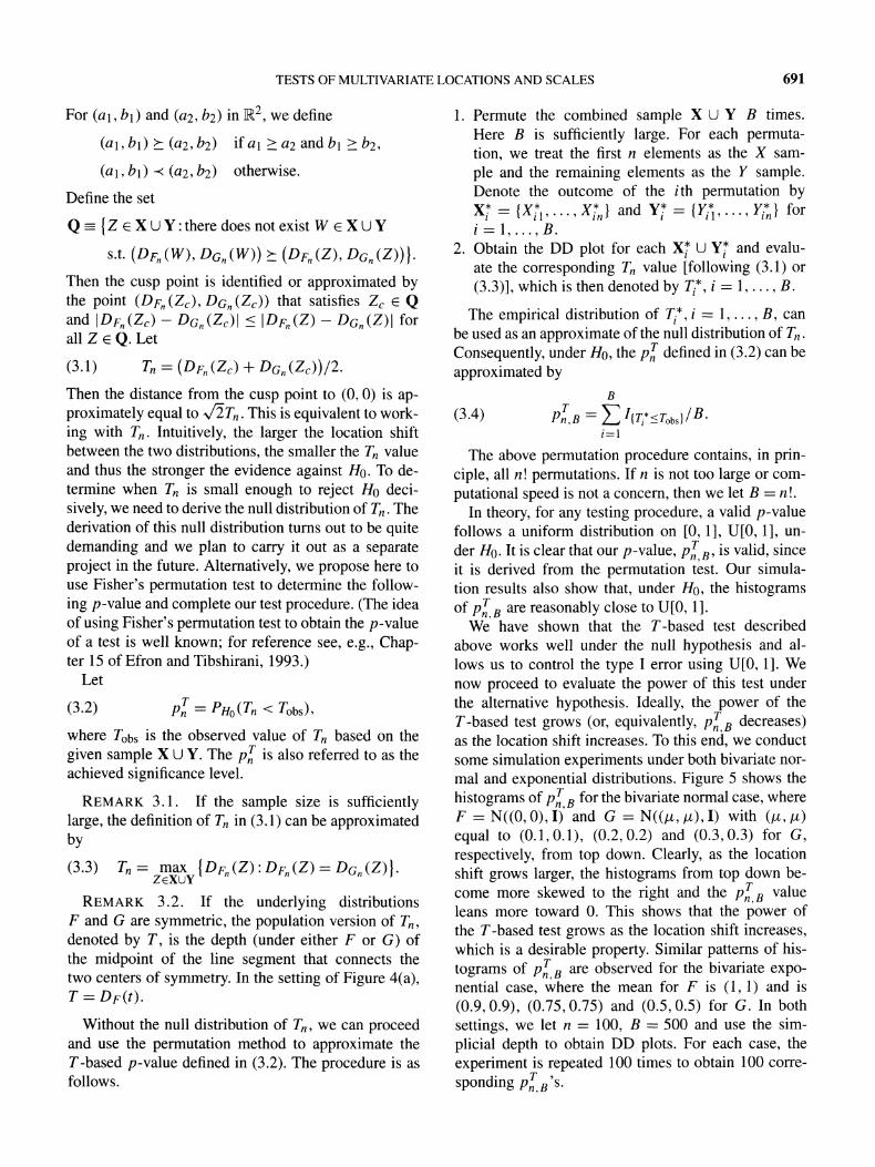
decreases) as the location shift increases. To this end, we conduct some simulation experiments under both bivariate nor- mal and exponential distributions. Figure 5 shows the histograms of

pnT B for the bivariate normal case, where

F = N((0, 0), I) and G = N((, /t), I) with (A, /t) equal to (0.1,0.1), (0.2, 0.2) and (0.3, 0.3) for G, respectively, from top down. Clearly, as the location shift grows larger, the histograms from top down be- come more skewed to the right and the pT'B value leans more toward 0. This shows that the power of the T-based test grows as the location shift increases, which is a desirable property. Similar patterns of his- tograms of

pnTB are observed for the bivariate expo-

nential case, where the mean for F is (1, 1) and is (0.9, 0.9), (0.75, 0.75) and (0.5, 0.5) for G. In both settings, we let n = 100, B = 500 and use the sim- plicial depth to obtain DD plots. For each case, the experiment is repeated 100 times to obtain 100 corre- sponding p7 B's. Pn,B

S

692 J. LI AND R. Y. LIU

0.0 0.2 0.4 0.6 0.8 1.0 Pn1

a

0.0 0.2 04 0.6 0.8 1.0

Pn3

FIG. 5. Histograms of pT B under Ha, where Ho: (i, /) = (0, 0)

and Ha :(/(, L) = (0.1,0.1), (0.2, 0.2) and (0.3, 0.3) (bivariate normal case).

3.2 M-Based Test: Monitor the Maximum

Depth Points

We next propose another test based on the DD plot for detecting a location change in two multivariate dis- tributions. This test statistic is more in the form of a location estimator. In the context of data depth, the location parameter of a distribution is defined as the deepest point (see, e.g., Liu, Parelius and Singh, 1999). If the two distributions F and G are identical, they should have the same deepest point. On the other hand, if there is a location change, the deepest point of the distribution F would no longer be the deepest point of the distribution G and thus it attains a smaller depth value w.r.t. G. The larger the location change is, the smaller this depth becomes. This trend can also be ob- served from the DD plots in Figures 2(b) and 4(b). This observation motivates our second test below, in which the test statistic monitors directly the depth values of the deepest points of the underlying distributions. Let

(3.5) Mn = min { DF (ZGn), DG, (ZF,) },

where ZG,

and ZF,0

are the deepest points among X U Y with respect to Gn and Fn, respectively.

REMARK 3.3. In theory, we may also consider other functions of the two depths such as the maxi- mum in (3.5). However, we choose to work with the minimum of the two depths, because the minimum is more sensitive to the location change and it can achieve more power.

We now proceed and carry out the test by determin-

ing its achieved significance level, defined as

(3.6) PnM

= PHo(Mn < Mobs).

Again, we turn to Fisher's permutation test to estimate the p-value pnm.

The procedure consists of the two steps outlined for the T-based test, except that each permutation replication is now used to evaluate the Mn as defined in (3.5). Denote by Mj* the Mn value ob- tained in the ith permutation. The p-value pn is then approximated by

(3.7) PnmB - E I{M

obs}/B. i=1

Discussions of the validity and power of the T-based test in terms of the proposed p-value apply similarly to the proposed pnB

based on the M-based test de- scribed above. Again, the histograms of the 100 simu- lated pnMB'S under the standard bivariate normal and

exponential distributions appear close to U[0, 1] un- der Ho, and they skew more to the right as the location shift widens, as observed in Figure 5.

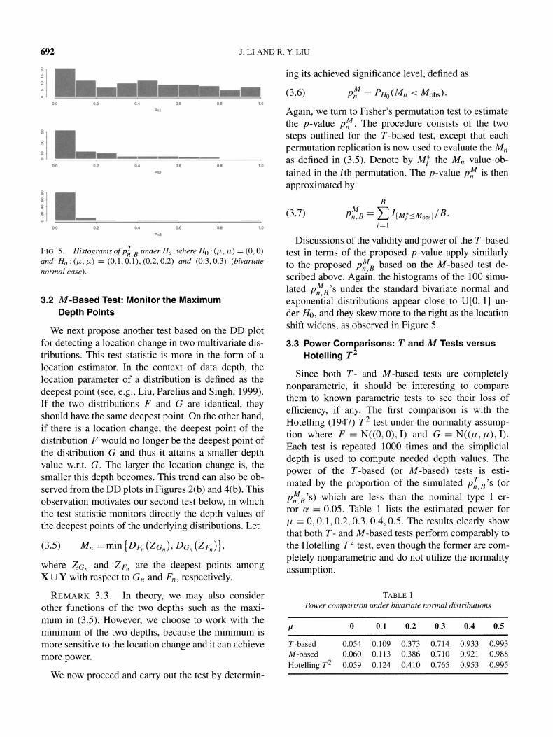
3.3 Power Comparisons: T and M Tests versus Hotelling T2

Since both T- and M-based tests are completely nonparametric, it should be interesting to compare them to known parametric tests to see their loss of efficiency, if any. The first comparison is with the Hotelling (1947) T2 test under the normality assump- tion where F = N((0, 0), I) and G = N((/, it), I). Each test is repeated 1000 times and the simplicial depth is used to compute needed depth values. The power of the T-based (or M-based) tests is esti- mated by the proportion of the simulated P,B's (or

PnM 's) which are less than the nominal type I er- ror a = 0.05. Table 1 lists the estimated power for

/t = 0, 0.1, 0.2, 0.3, 0.4, 0.5. The results clearly show that both T- and M-based tests perform comparably to the Hotelling T2 test, even though the former are com- pletely nonparametric and do not utilize the normality assumption.

TABLE 1 Power comparison under bivariate normal distributions

A 0 0.1 0.2 0.3 0.4 0.5

T-based 0.054 0.109 0.373 0.714 0.933 0.993 M-based 0.060 0.113 0.386 0.710 0.921 0.988

Hotelling T2 0.059 0.124 0.410 0.765 0.953 0.995

TESTS OF MULTIVARIATE LOCATIONS AND SCALES 693

TABLE 2 Power comparison under bivariate Cauchy distributions

I 0 0.1 0.2 0.3 0.4 0.5

T-based 0.052 0.060 0.114 0.154 0.214 0.350 M-based 0.046 0.072 0.118 0.214 0.324 0.522

Hotelling T2 0.020 0.010 0.020 0.034 0.022 0.052

We also conducted the same comparison study for the bivariate Cauchy distributions with the location pa- rameter (it, it). Clearly, both T- and M-based tests outperform the Hotelling T2. This can be attributed to the fact that the first two tests using the simplicial depth are moment-free approaches and thus more suitable for testing location parameters not derived from moments, such as in the case of Cauchy distributions. The results in Table 2 seem to suggest also that the M-based test is more powerful than the T-based test in the Cauchy case. We plan to investigate further the difference be- tween the T- and M-based tests, including their robust- ness properties as well as their capability to cope with asymmetric underlying distributions.

4. RANK TESTS FOR SCALE EXPANSION OR CONTRACTION

Let, again, X - {Xi, ..., Xn} ,- F and Y - { Y1,..., Y, } -- G be two given samples in Rk. Assume that F and G are identical except for a possible scale dif- ference. For simplicity, assume that we are interested in testing if G has a larger scale in the sense that the scale of G is an expansion of that of F. In other words, the hypotheses of interest are

Ho: F and G have the same scale (4.1)

Ha :G has a larger scale.

Combine the two samples, that is, let W - { W1, W2, .., Wn+m} -{X1, ...,Xn, Y1,..., Ym}. If G has a

larger scale, then the Xi's are more likely to clus- ter tightly around the center of the combined sample, while the Yi's are more likely to scatter at outlying positions. This outlyingness can be easily captured by data depth. Following this observation, Liu and Singh (2003) developed depth-induced rank tests to compare scales among two or multiple multivariate samples. In this paper we provide a brief review of their rank test for two samples. Detailed discussions and justifications can be found in Liu and Singh (2003).

4.1 Larger Scale-More Outlying Data- Smaller Ranks

Using any measure of depth, we can compute the

depth values of the points in the combined sample W. We then assign ranks to the combined sample W ac-

cording to the ascending depth values, namely, lower ranks to the points with lower depth values. Specif- ically, we let r(Yi) be the center-outward rank of Yi within the combined sample, that is,

r(Yi) = #{Wj E W: Dn+m(Wj) < Dn+m(Yi),

(4.2) j =l, 2,...,n + m},

and we let the sum of the ranks for the sample Y be

m

(4.3) R(Y)= r(Yi). i=1

Here, Dn+m (0) is the sample depth value of * mea- sured w.r.t. {W1, W2,..., Wn+m}. Under Ho, if there are no ties, {r(Y1), ..., r(Y,m))) can be viewed as a ran- dom sample of size m drawn without replacement from the set { 1, ... , n +m }. If Ha is true, then the Yi's tend to be more outlying, and thus assume smaller depth val- ues and thus smaller ranks. In other words, we should

reject Ho if the rank sum R (Y) is too small. The critical values for carrying out this test can be implemented us-

ing the Wilcoxon rank-sum procedure as if one is test-

ing a negative location shift in the univariate setting. For a review of the Wilcoxon rank-sum test and its tab- ulated distributions for different sample size combina- tions, see, for example, Hettmansperger (1984). When n and m are sufficiently large, following the large- sample approximation, we can reject Ho if R* < z, for an a-level test. Here

( R(Y) - (m(n + m + 1)/2} (4.4) R+ m + 1) {nm(n + m + 1)/12}1/2

The depth ranking of sample points, due to its center- outward nature, often leads to ties, especially in high dimension cases. To use the tables provided for the Wilcoxon rank-sum test, we may consider the random

tie-breaking scheme. However, we can actually carry out the test and obtain its exact p-value without break-

ing ties by the following approach. Since powerful computing facilities are easily available nowadays, we can use computers to obtain the exact distributions for the observed ranks, with or without ties. Specifically, we permute all the observed ranks (possibly including ties), calculate the sum of the first m ranks in each per- mutation, and finally tabulate such rank sums and their

694 J. LI AND R. Y. LIU

corresponding frequencies in the total number of per- mutations. This distribution allows us to determine the exact p-value of our test, which is simply the propor- tion of the rank sums which are less than or equal to the observed rank sum in (4.3). As an illustrative example, we assume that n = m = 2 and that the ranks for the combined sample turn out to be {1, 2, 2, 4) with a tie. The sampling distribution of the rank sum R -- R(Y) is

P(R = 3) = 8/24, P(R = 4) = 4/24, (4.5)5) = 4/24, P(R =6) = 8/24.

P(R = 5) = 4/24, P(R = 6) = 8/24.

Therefore, if the observed rank sum is 4, then the p-value is P(R < 4) = 0.5. For large samples, the distribution of the rank sum can be approximated by considering large enough numbers of permutations. In Table 3, we present some simulation results to examine the power of the rank test. Here the samples are from three bivariate distributions: Cauchy, normal and expo- nential, each with the component variance o2. We as- sume n = m, and consider n = 20 and n = 30. In each case 5000 random permutations of the observed ranks were used to approximate the sampling null distribu- tion, and the rank test at significance level 0.05 was repeated 1000 times.

The results in Table 3 show that the power achieved by the rank test for scale expansions is quite re- spectable, especially in the nonnormal cases. A power comparison between the above rank test and a X2 test under the normality assumption can be found in Liu and Singh (2003). The results there show some minor loss of efficiency of the rank test in the normal case. Liu and Singh (2003) also discussed in detail the prop- erties of this rank test as well as several approaches for dealing with large numbers of ties in the depth rank- ing. Moreover, they also generalized the rank test to the case of multiple samples.

Note that the rank test described above can be viewed as the multivariate generalization of Ansari- Bradley and Siegel-Tukey tests for testing the equality

TABLE 3 Simulated power of the rank test for scale expansions (a = 0.05)

n = 30 n =20

a Cauchy Normal Exp Cauchy Normal Exp

1-1 0.056 0.044 0.049 0.054 0.051 0.043 1-1.2 0.345 0.325 0.218 0.261 0.242 0.188 1-2 0.996 0.994 0.940 0.966 0.940 0.813

of variance in the univariate setting. Both tests try to assign smaller ranks to the data points which are more outlying toward two tails, although the Siegel-Tukey test avoids ties by alternating ranks.

If we are interested in testing whether or not G has a smaller (contracted) scale, then we should reject the null when the rank sum is too large.

The rank test above is easily implementable and is completely nonparametric. Its p-value yields a decisive decision rule. The test result can be independently veri- fied visually by two graphical tools: One is the DD plot [see Figure 3(a) and the discussion in Section 2.2]; the other is the scale curve introduced by Liu, Parelius and Singh (1999). The sample scale curve derived from a sample of size n is defined as

(4.6) Sn(p) = volume {C,,p) for 0 5 p < 1.

Here Cn,p is the convex hull that contains the [npl deepest points. Roughly speaking, the scale curve measures the volume expansion of the nested depth contours, as seen in Figure 1, as the contours grow to enclose more probability mass. This plot of S,n (p) ver- sus p shows the scale of the distribution as a simple curve in the plane, which is easily visualized and in- terpreted. When comparing the scales of two samples, if one scale curve is consistently above the other, then the sample with the higher scale curve is more spread out and thus has a larger or expanded scale.

5. APPLICATION TO AIRLINE PERFORMANCE DATA

We apply all tests described so far to an analysis of an airline performance data set collected by the FAA. It consists of several monthly performance measures of the top 10 air carriers from July 1993 to May 1998. The performance measures include the fractions of noncon- formity in airworthiness and operation surveillance. A small nonconformity fraction is a desirable feature. Several depth-induced multivariate control charts (Liu, 1995; Cheng, Liu and Luxh0j, 2000) have been used to monitor and compare the performances of all 10 airlines. For illustration, the T- and M-based tests are used to determine whether there is a significant difference in location (referred to as expected target performance in the aviation safety domain) in the dis- tributions that underlie two air carriers. In comparing air carriers 1 and 4, their scatter plots in Figure 6(a) show a clear location shift to the upper right in car- rier 4. The deepest point of carrier 4, marked by a solid triangle, is more to the upper right than that of carrier 1,

TESTS OF MULTIVARIATE LOCATIONS AND SCALES 695

(a) (b) o 0

o Carrier 1 o0 Carrier 4 O

t

* deepest point for Carrier 1 o 00 0

deepest point for Carrier 4 0

00 00 00 A A

o A AoA"o 0o0

A 0

SAoA A o00 0 0

0 0

0 00 0 0 0 0 0 00 0

00

00

&0

0.04 0.06 0.08 0t1 0.12 0.t4 01 0.0 0.05 0 .0t

0.t5 0.20 0.25 0.30

AW ODF

FIG. 6. (a) Scatter plot and (b) DD plot for carriers 1 and 4.

marked by 9. The DD plot for the two carriers in Fig- ure 6(b) has the cusp point pulled down toward (0, 0) to the midrange of the plot and clearly indicates a location difference in the two distributions. Using both T- and M-based tests, we found the approximated p-values to be nearly 0, which confirms a significant location shift in the two distributions.

In judging airline performance, in addition to ex- amining the expected target performance (i.e., the lo- cation of the distribution) of the airlines, the stability of the performance within the airlines is also a major concern. This measure of stability is simply the mea- sure of scale or variation of the performance distrib- ution. Thus, comparing performance stability amounts to comparing the scales of distributions. Larger or more expanded scales mean less stable performance. We pro-

ceed and compare the scales of carriers 1 and 4. The p-value is 0.00038 using the test statistic in (4.3), which clearly supports the conclusion that carrier 4 has a larger scale than carrier 1. In other words, the per- formances of carrier 4 are more scattered and hence less stable. This same conclusion can also be reached by examining the two graphs in Figure 7. Figure 7(a) is the DD plot of carriers 1 and 4 after centering the data respectively at their deepest points, removing the effect of location difference. It shows a pattern which combines Figure 3(a) and (b). This suggests that there are both scale and skewness differences between the two carriers. Figure 7(b) displays the scale curves, as defined in (4.6), of four carriers. Obviously, the scale curve of carrier 4 lies consistently above all others, including that of carrier 1. The findings are also sup-

(a) (b) 400

00 03 300 0o

230 0--C • 0 0o

0 0 o 0 300 0 o 000

0 0e

0 o0

o 0 0 250

0 Oo 0

o

o

o

00 0 0 0000

200-

.0

0 0 000.

0 0 005 0 020 0.25 0.30 0000 0 160

0 000 0 0 0 100

L o 0 00

0. I.5 I I

02 021.00.0 0.1 0.2 0.3 0.4 0.5 0.6 0.7 0.8 0.9 1.0

OF p fractioe

FIG. 7. (a) DD plot for carriers 1 and 4 after centering. (b) Scale curves for air carriers.

696 J. LI AND R. Y. LIU

ported by the scatter plots in Figure 6(a), which show more scattered data for carrier 4. In summary, the per- formance of carrier 4 is inferior to that of carrier 1, in that carrier 4 has significantly higher target nonconfor- mity ratios and it is also much less stable overall. Possi- ble causes should be identified and corrective measures should be taken.

6. CONCLUDING REMARKS

Although our illustrative examples are in R2, all tests discussed in this paper apply to any dimension.

The DD plot of the rank test in Section 3 can be con- structed using any notion of data depth which is affine- invariant. Some notions of depth may be more suitable than others in capturing a certain feature of a distri- bution. For example, if the underlying distribution is close to elliptical, then it is more efficient to use the Mahalanobis depth. Otherwise, more geometric depths such as the simplicial depth or the half-space depth (Tukey, 1975) may be more desirable since they do not require specific distributional structures or moment conditions. Details on some of these conditions for dif- ferent depths can be found in Liu and Singh (1993) and Zuo and Serfling (2000). Note that it can be shown that the M-based test using Mahalanobis (1936) depth is as- ymptotically equivalent to the Hotelling T2 test when comparing elliptical distributions. In other cases, the M-based test is more robust.

Concerning the issue of computational feasibility in computing depth, although the exact sample simpli- cial depth value in any dimension can be computed by solving a system of linear equations, more efficient algorithms are desirable. Rousseeuw and Ruts (1996) provided an efficient algorithm for computing both the simplicial and the half-space depths in R2. Developing efficient algorithms in the case of higher dimensions has recently generated much interest in computational geometry. It is reasonable to expect rapid progress in this direction.

Some depth rank tests have been proposed by Liu and Singh (1993) for testing simultaneously location and scale changes. It may be worthwhile to compare these rank tests separately with the T-based and M- based tests for testing location changes, and with the rank test described in (4.3) for testing scale changes.

Several graphical diagnostic tools stemming from DD plots for the two-sample problem have been pro- posed by Hettmansperger, Oja and Visuri (1999) and Liu, Parelius and Singh (1999). Their associated infer- ences need to be developed to make the graphical tools rigorous tests. Combining proper statistics derived from graphical tools with the permutation test idea may prove to be a helpful step in developing these tests.

ACKNOWLEDGMENTS

This research is supported in part by grants from the National Science Foundation, the National Security Agency and the Federal Aviation Administration.

REFERENCES

CHENG, A., LIU, R. and LUXHOJ, J. (2000). Monitoring mul- tivariate aviation safety data by data depth: Control charts and threshold systems. IIE Trans. Operations Engineering 32 861-872.

DONOHO, D. and GASKO, M. (1992). Breakdown properties of lo- cation estimates based on half-space depth and projected out- lyingness. Ann. Statist. 20 1803-1827.

EFRON, B. and TIBSHIRANI, R. (1993). An Introduction to the Bootstrap. Chapman and Hall, London.

HETTMANSPERGER, T. (1984). Statistical Inference Based on Ranks. Wiley, New York.

HETTMANSPERGER, T., OJA, H. and VISURI, S. (1999). Discus- sion of "Multivariate analysis by data depth: Descriptive sta- tistics, graphics and inference," by R. Liu, J. Parelius and K. Singh. Ann. Statist. 27 845-854.

HOTELLING, H. (1947). Multivariate quality control: Illustrated by the air testing of sample bomb sight. In Selected Techniques of Statistical Analysis for Scientific and Industrial Research, and Production and Management Engineering (C. Eisenhart, M. Hastay and W. Wallis, eds.) 111-184. McGraw-Hill, New York.

LIu, R. (1990). On a notion of data depth based on random sim- plices. Ann. Statist. 18 405-414.

LIu, R. (1995). Control charts for multivariate processes. J. Amer Statist. Assoc. 90 1380-1387.

LIU, R., PARELIUS, J. and SINGH, K. (1999). Multivariate analy- sis by data depth: Descriptive statistics, graphics and inference (with discussion). Ann. Statist. 27 783-858.

LIu, R. and SINGH, K. (1993). A quality index based on data depth and multivariate rank tests. J. Amer Statist. Assoc. 88 252-260.

LIU, R. and SINGH, K. (2003). Rank tests for comparing multivari- ate scale using data depth: Testing for expansion or contrac- tion. Unpublished manuscript.

LIu, R., SINGH, K. and TENG, J. (2004). DDMA-charts: Non- parametric multivariate moving average control charts based on data depth. Allg. Stat. Arch. 88 235-258.

MAHALANOBIS, P. (1936). On the generalized distance in statis- tics. Proc. Nat. Acad. Sci. India 12 49-55.

MOSLER, K. (2002). Multivariate Dispersion, Central Regions and Depth: The Lift ZonoidApproach. Lecture Notes in Statist. 165. Springer, New York.

ROUSSEEUW, P. and RUTS, I. (1996). Algorithm AS 307: Bivariate location depth. Appl. Statist. 45 516-526.

TUKEY, J. (1975). Mathematics and the picturing of data. Proc. In- ternational Congress of Mathematicians 2 523-531. Canadian Math. Congress, Montreal.

Zuo, Y. and SERFLING, R. (2000). Structural properties and con- vergence results for contours of sample statistical depth func- tions. Ann. Statist. 28 483-499.