living arrangements of the elderly in china: evidence from … · 1 living arrangements of the...
TRANSCRIPT

1
Living Arrangements of the Elderly in China:
Evidence from the CHARLS National Baseline
Xiaoyan Lei Peking University
John Strauss University of Southern California
Meng Tian Peking University
Yaohui Zhao Peking University
Revised April 2013
Revised October 2012 This research is supported by the US National Institute of Aging, the Natural Science Foundation
of China, Fogarty International Center, and the World Bank.
2
Abstract
Declining fertility in China has raised concerns about elderly support, especially when public support is inadequate. However, using rich information from the nationally representative China Health and Retirement Longitudinal Study (CHARLS) baseline survey fielded in 2011-12, we find that roughly 39% of Chinese aged 60 and over live with a child; living with a male child being strongly preferred. However another 34% have a child living in the same immediate neighborhood and 14% in the same county; only 5% have the nearest child living outside the same county as the parent and another 7% have no living children. Living alone or with only a spouse is common among Chinese elderly, 48% in our sample, much larger than is true in other Asian countries. Urban elderly residents are more generally likely to live with their children. Children with high levels of income are less likely to live with their parents or to live nearby, but if parents have higher income, one of their children is more likely to be living with them or nearby. We also find that among non-co-resident children, those living close by visit their parents more frequently and have more communications by phone, email, text messages and regular mail. On the other hand, children who live farther away are more likely to send financial and in-kind transfers and send larger amounts. Children thus substitute amongst themselves between providing support to parents in the form of time versus money.
Keywords: living arrangement, co-residence, proximity of children, CHARLS

3
1. Introduction
Population is rapidly aging in China. In 2000, people 60 and older accounted for 10% of the
population. The ratio rose to 13.3% in 2010 and is expected to reach 30% in 2050 (United Nations,
2002). Unlike in developed countries where almost all elderly have access to publicly provided
social security, the family has been the main source of support for Chinese elderly, especially in
rural areas where the majority of Chinese elderly reside. In recent decades, however, the number
of children has declined rapidly, as the total fertility rate has fallen from 6 in the end of the 1960s
to under 2.0 today. In addition, rural young people have moved into cities in large numbers as part
of the process termed “history’s greatest migration in the world”. These trends have raised
questions regarding the reliability of family as the provider of elderly support in China.
This concern is echoed by empirical evidence which shows that Chinese elderly are
increasingly living alone or only with a spouse. Pamler and Deng (2008), using the China
Household Income Project (CHIPs) data collected in 1988, 1995, and 2002, show that persons 60
and older, especially those in urban areas, are increasingly more likely to live with their spouses
rather than in intergenerational households with their children. They conjecture that the trend is
due to the increasing availability of pensions, however,rapidly rising incomes and savings over
this period, plus improved health over younger birth cohorts no doubt contribute to this trend as
well. Meng and Luo (2008), using the urban sample of CHIPs, also show that the fraction of
elderly living in an extended family in urban China declined significantly over the study period.
They also cite the housing reform during the 1990s, which increased housing availability and
hence allowed elders who preferred to live alone to do so. Using population census data of 1982,
1990 and 2000, Zeng and Wang (2003) present a similar pattern and attribute it to tremendous
fertility decline and significant changes in social attitudes and population mobility. Figure 1
shows that the rate of living alone or only with a spouse further declined in 2005 compared to
4
2000.
What do we infer about the welfare of the elderly from this trend of living away from
children? Benjamin, Brandt, and Rozelle (2000) find that elderly person living alone are worse off
in terms of income than those living in an extended household, and the welfare implication is
even stronger when we recognize that elderly in simple households also work more. Sun (2002)’s
research on China’s contemporary old age support suggests that living away from children
constrains the elderly in receiving help with daily activities. Silverstein et al. (2006) find for a
sample of rural Chinese elderly in Anhui province, that parents who live with grandchildren,
either in three or skipped-generation households, have better psychological well-being than those
who live by themselves, or even with children, but without grandchildren.
A similar trend of elderly living alone has been noted in the United States where the
proportion of elderly living independently increased markedly in the 20th century (Costa, 1997;
McGarry and Schoeni 2000; Engelhardt and Gruber 2005). While the literature has noted that
living alone is associated with poverty, a higher level of depression symptoms and more chronic
diseases (Agree 1993; Saunders and Smeeding 1998; Victor et al. 2000; Kharicha et al. 2007;
Wilson 2007; Greenfield and Russell 2010), the economic literature has in general viewed this
trend as utility enhancing for the elderly, because independence, or privacy, is a normal good
(Doty 1986; Martin 1989; Kotlikoff and Morris 1990; Mutchier and Burr 1991; Tomassini et al.
2004). For example, Costa (1998) finds that prior to 1940, rising income substantially increased
demand for separate living arrangements, and therefore, was the most important factor enabling
the elderly to live alone in the United States. McGarry and Schoeni (2000) analyze the causes of
the increasing share of elderly widows living alone between 1940s and 1990s, and indicate that
income growth, especially increased social security benefits, was the single most important factor
causing the change in living arrangements, accounting for nearly two-thirds of the rise in living

5
alone. With a more recent data from the Current Population Survey 1980-99, Engelhardt and
Gruber (2005) find that living arrangements are still very income sensitive, particularly for
widows and divorcees, and conclude from the results that privacy is valued by the elderly and
their families.
What we find lacking in the literature is that living alone and getting the support from the
family are viewed as mutually exclusive, that living alone means not getting the help and in order
to get the care from the family they need to live together. However, a paper by Zimmer and
Korinek (2008) shows in China, using the Chinese Longitudinal Healthy Longevity Survey, that a
large fraction of Chinese elderly who do not live with their adult children, have children living in
very close proximity, within the same neighborhood. This is a different pattern than they find in
other Asian countries that they examine. They then explore how this probability is influenced by
the number of children, rural/urban residence, education and some other covariates. Bian, Logan,
and Bian (1998) find a similar co-residence pattern using data from two cities (Shanghai and
Tianjin) in 1993; that although most elderly still lived with children, many of them also had
children living nearby, providing regular non-financial assistance and maintaining frequent
contact. Giles and Mu (2007) also provide some evidence on this tendency, though it is not the
focus of their paper.
In this paper, we further examine how Chinese families reconcile these two objectives, using
the first truly nationally representative survey of the Chinese elderly, the national baseline wave
of the China Health and Retirement Longitudinal Study (CHARLS). We find that many Chinese
elderly live alone or only with a spouse, but at the same time, most of them have a child living
nearby to guarantee care when needed. The first goal of this paper is to depict an updated and
broad picture of the living arrangements of the Chinese elderly and to look at how many elderly
parents living alone actually have access to children, i.e., have children living nearby. Secondly,
6
we aim to shed some light on what determines the living arrangements of Chinese families with
elderly parents, especially the proximity of children. Finally, we examine the tradeoff between
living arrangements and other forms of elderly support including the frequency of visits and
financial transfers. We find that the increasing trend in living alone is accompanied with a rise
in living close to each other. This type of living arrangement helps to solve the conflict between
privacy/independence and family support. This is confirmed in further investigation: children
living close by visit their parents more frequently. We also find that children who live far away
provide a larger amount of net transfers to their parents, a result consistent with responsibility
sharing among siblings. Sons, especially last- and first-borns, are more likely to live with their
parents than daughters or middle born sons. Children with higher incomes are more likely to live
away, out of the county, but also more likely to provide financial transfers and larger transfers.
The remainder of the paper is organized as follows. The next section describes our data.
Section 3 presents the patterns of China’s elderly living arrangements. Section 4 discusses the
empirical results on the determination of elderly living arrangements. Section 5 concludes.
2. Data
We use the CHARLS 2011-12 national baseline data, which is described in detail in Zhao et
al. (2013). CHARLS was designed after the Health and Retirement Study (HRS) in the US as a
broad-purposed social science and health survey of the elderly in China. A pilot survey was
conducted in Gansu and Zhejiang provinces in July-September 2008 and resurveyed in the
summer of 2012, and the national baseline was conducted in July 2011-March 2012. The
CHARLS sample is representative of people aged 45 and over living in households in 150
counties in 28 provinces across China.
The sampling design of the 2011 wave of CHARLS was aimed to be representative of
residents 45 and older in China. CHARLS randomly selected 150 county-level units by PPS

7
(probability proportional to size), stratified by region, urban/rural and county-level GDP.1 Within
each county-level unit, CHARLS randomly selected 3 village-level units (villages in rural areas
and urban communities in urban areas) by PPS as primary sampling units (PSUs). Within each
PSU, CHARLS then randomly selected 80 dwellings from a complete list of dwelling units
generated from a mapping/listing operation, using augmented Google earth maps, together with
considerable ground checking. In situations where more than one age-eligible household lived in a
dwelling unit, CHARLS randomly selected one. From this sample for each PSU, the proportion of
households with age-eligible members was determined, as was the proportion of residences that
were empty. From these proportions, and an assumed response rate, we selected households
from our original PSU frame the number sampled chosen to obtain an targeted number of 24
age-eligible houeseholds per PSU. Thus the final household sample size within a PSU depended
on the PSU age-eligibility and empty residence rates. Within each household, one person aged 45
and older was randomly chosen to be the main respondent and their spouse was automatically
included. Based on this sampling procedure, 1 or 2 individuals in each household were
interviewed depending on marital status of the main respondent. The total sample size is 10,257
households and 17,708 individuals. The overall household response rate was 80.5%; 71.7% in
urban areas and 95.1% in rural areas. These response rates are higher than the rates in the US and
Europe for first wave of population-based surveys.
Following the protocols of the HRS international surveys, the CHARLS main questionnaire
in the 2011-12 survey consists of 7 modules, covering demographics, family background, health
status (including physical and psychological health, cognitive functions, lifestyle, and behaviors),
socioeconomic status (SES), and environment (community questionnaire and county-level policy
1 The counties represent all Chinese provinces except Hainan, Ningxia, which had no counties sampled, and Tibet, Hong Kong, Macau, and Taiwan, which were not included in the sample.

8
questionnaire) (Zhao et al. 2013). All data were collected in face-to-face, computer-aided personal
interviews (CAPI).
In the family module, all CHARLS respondents were asked how many living children they
have. For each child, CHARLS collected information on a variety of characteristics: sex, birth
year and month, biological relationship with respondent and residence. The residence of the child
is categorized as follows: (1) this household, (2) adjacent dwelling or same courtyard, (3) another
house in this village or community, (4) another village or community in this county or city, (5)
another county or city in this province, (6) another province, and (7) abroad. This information
enables us to describe the living arrangements in a more detailed way than the previous literature.
Other information collected includes each child’s education level, income category (an ordinal
measure), marital status, working status, occupation and number of children. For parents
(respondents), we have detailed demographic information, income and wealth measures, and rich
health measures. More details about the variables we use are provided in Section 4. With this rich
pool of information, we can use multivariate estimation to identify the determinants of elderly
living arrangements and investigate joint decisions between parents and children.
3. Patterns of Elderly Living Arrangement
We examine the living arrangements of elderly respondents, similar to the previous literature,
but with special consideration to the proximity of child. We divide elderly living arrangements
into six categories, not all of them mutually exclusive: (1) living alone or with only spouse, (2)
living with one or more adult children, (3) living alone, but with one or more children in the same
village or community, (4) living alone, but with one or more children in the same county, (5)
living alone without any child in the same county, and (6) childless. We also examine, classify
respondents, if they live with others besides their spouse, as living with children-in-law but not
including living with a child (who may be working in a different place), living with grandchildren

9
but not children, and other living relationships.
We restrict our attention to elderly households with at least one respondent 60 and older.2
Table 1 presents an overall picture of the elderly households’ living arrangements at the time of
the survey.3 Wherever needed, the characteristics (e.g., gender) of the main respondent are used.
From this table, we can see that basically 47.5% if all elderly respondents and spouses live alone
or with only a spouse. This is considerably higher than found in other Asian countries, which
averages only 25% (United Nations, 2011). Some 39% of all elderly respondents are living with
one or more adult children. A small number of them (6.8% of all) are childless, most of those men.
Another 7.6% live with grandchildren, but not children. Those grandchildren span ages from
adults who could care for their grandparents to very young who are being cared for by their
grandparents. Another 2.3% live with children-in-laws, but not their children. Of those who
have child(ren) but do not live with them, 63.5% (34.4/54.2) have at least one adult child living in
the same village/community, meaning that they should have access to care from child(ren). Even
for those without access to a child in the same village, 72.7% (14.4/19.8) have at least one child
living in the same county. Only 5.8% of elderly with children, and 12.2% of all elderly do not
have a child within the same county. This indicates that failing to account for the proximity of
children will exaggerate the plight of the elderly in terms of care from children.
In general, women are a little more likely to live with or close to their children than men;
those from western provinces and from rural areas are slightly more likely to do so than those
from eastern and middle provinces and urban areas. Meanwhile, men, those from eastern
provinces and urban areas are more likely to be childless than their corresponding counterparts.
2 We also exclude a small number of households with respondents who are separated couples, or are rotating parents because the living arrangements of such households are hard to define. Later on, in order to focus on living arrangement of elderly parents and their adult children, we further restrict to those with at least a child 25 or older and is not currently in school 3 All numbers in Table 1 use sample weights that also adjust for household non-response. See Zhao et al. (2013) for a discussion of sample weights.

10
Figure 2 shows the age patterns of elderly living arrangement without taking account of how
close the children live. Two lines, one living alone or with spouse only, the other living with one
or more adult child, are displayed. We see that the probability of living alone or only with spouse
increases with age until 77-78 and then decreases, and the probability of living with children
declines and then increases correspondingly.4 This pattern reflects that children may move back
to meet their elderly parents’ needs for care. Being more likely to live alone as age increases (up
to a point), is not so unusual. Based on a comprehensive dataset collected from 50 countries
across five continents, the United Nations (2005) shows that the likelihood of living alone
actually increases at advanced ages. However, a different story emerges when we examine the
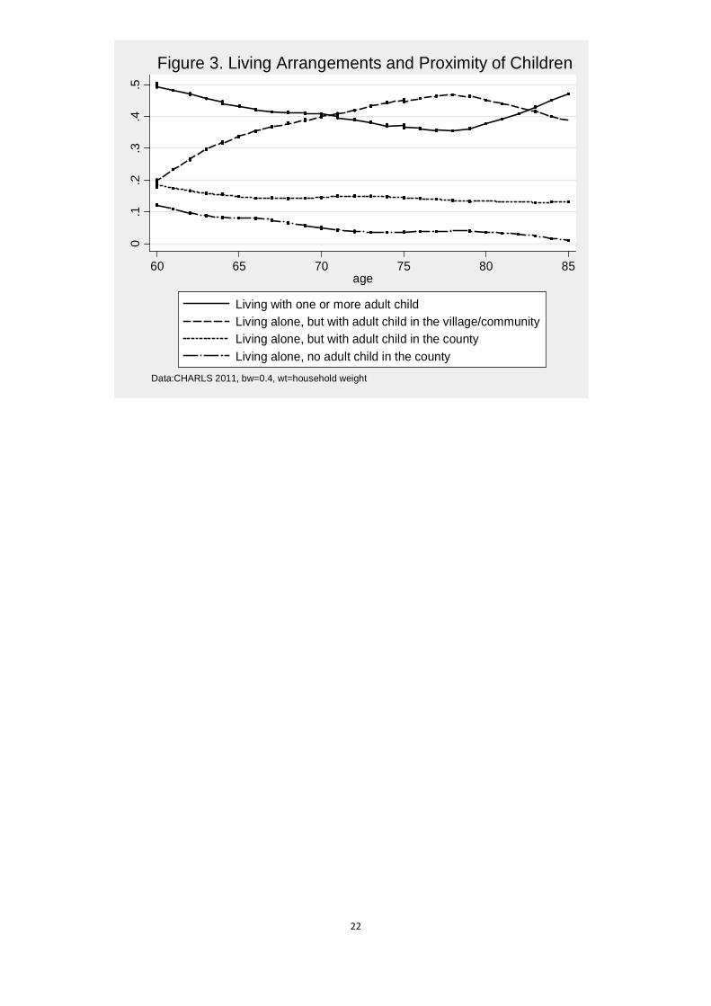
pattern in more detail. As shown in Figure 3, the decline in the proportion of co-residency by age
is fully compensated by the increasing share of proximate child(ren). The likely story is that when
children mature and obtain independence from their parents, they do not abandon the parents.
They move out but live nearby so that the care needs of parents are met. This is further evidence
that looking at the proximity of children is valuable in understanding the welfare of the elderly.
Table 2 shows characteristics of the respondents (parents) by the living arrangement of the
households, i.e., whether they are living with a child, have a child living in the same county, or far
away.5 If the respondents are couples in the household, maximum age, maximum education, and
the health condition of the person in worst health is reported because these measures may be more
relevant to living arrangement decisions. Nine percent of households have a single male
respondent, 23% have a single female respondent, and the remaining 67% are couples. On
average, the maximum age of the elderly parents is about 70. Hence the average parent was born
4 Note that this pattern differs from what we get from the census data (Figure 1), which presents a downward trend of living alone with age before 76-77. The difference may result from the different definitions of “household”. CHARLS is very meticulous about its definition of “households.” Household members are defined as those families that live under the same roof, share food and other expenses. The Census, on the contrary, has no clear definition of “households.” The determination of a “household” is largely dependent on household registration. We think that our definition is more appropriate. 5 We treat living in the same county as living nearby because the distance within a county allows for daily communication.
11
around 1942, which means they would have been 38 in 1980, when the One-Child Policy started
and in their late 20s and early 30s during the family planning programs established during the
early 1970s. This absence of exposure to the stronger family planning policies is reflected in the
number of surviving children, which is 3.29. Almost half, 48%, are from urban areas. Regarding
health status, 22% rate their health as being very poor. Thirty-seven percent report having any
ADL or IADL difficulties. The education level of the elderly parents is generally very low.
Twenty-five percent are illiterate, and 45% have a primary education either formally or
informally.6 The annual pre-transfer income for the elderly household is 7,981 RMB, but with a
very large standard deviation. Seventy two percent of the elderly parents currently own a house.
Parents living with a child tend to be more heavily widowed, female, illiterate, and less likely to
own their own house.
Table 3 shows the characteristics of the adult children aged 25 and older. On average, they are
41.5 years old, with 47% being daughters and 53% sons. The average number of their children
younger than 16, so grandchildren of our respondents is 1.0. The educational level of the children
is much higher than their elderly parents. Only 9% are illiterate, 39% have completed primary
school, 31% have a middle school education, and the remaining 20% have an education of high
school and above.
Table 3 also offers a detailed comparison between children living in the same household,
children within the same county and children who live faraway. The co-resident children are
generally younger than those who are non-co-resident. Parents are much more likely to live with
sons, particularly their youngest sons. On average, co-resident children have more children (less
than 16 years old) of themselves than the non-co-resident children.
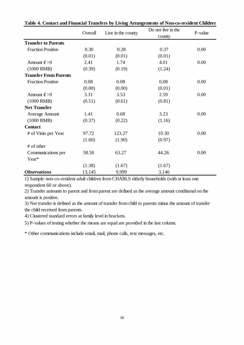
Table 4 shows the transfers provided by and to children with different living arrangements:
6 Though these education levels are considerably higher than that of the respondent’s parents.
12
living in the same county or far away. The probability of financially transferring to parents is
lower for those living in the same county, and the amount of gross transfers to parents is far
higher for those children who live far away. Getting transfers from parents is equally likely no
matter how close the child lives, and the closer child on average receives higher transfers from
parents, which is perhaps used in weddings and housing purchase, although our data do not show
this. On net, children give far more transfers to parents than they receive. This is a different
pattern that one sees in the US or Europe, where net transfers are from elderly parents to children,
but is similar to the pattern observed in other low income countries. As expected, the children
who live nearby are more likely to visit their parents, or to have other communications with their
parents, possibly for the purpose of providing more help.7 On the other hand children who live
farther away provide higher net transfers to their parents than do children who live nearby.
To sum up the results in this section, we find that although more than half of the elderly
CHARLS respondents live by themselves, most of them indeed have access to child assistance.
The probability of elderly living alone increases as the elderly ages, to a point, and then declines,
but when it is increasing in age, it is mostly compensated by the presence of a child in the same
village/community or county. Furthermore, those nearby children pay more frequent visits to
their elderly parents, while those far away are more likely to provide transfers and to provide a
higher amount of net transfers on average.
4. Correlates of Elderly Living Arrangement
In this section, we examine more systematically the predictors of elderly living arrangements.
The rich information on parent and child characteristics together allow us to group the data at
child level, that is, to treat each child as one observation. This will enable us to use both
multinomial logit and family fixed-effects models, the family fixed effects to control for
7 Other communications include email, mail, phone calls, text messages, and so forth.

13
unobserved heterogeneity at the family level.8
We restrict our parent respondents who are aged 60 or above, with at least one child who is
aged 25 and older and not a student. It is rarely the case that when we have data on a parent and
the spouse, that they do not live together. To count them as two observations would not be
appropriate so in those cases, we treat them as a single observation and use the main respondent’s
data. Our sample includes 4,697 respondents and correspondingly 15,418 in the child sample.
In the following, we will separately report the results from estimation on co-residence and on
proximity, and then examine the associations of living arrangement with visit frequencies and
transfers.
4.1. Correlates of Living Arrangements
Whether or not the elderly live with or close to their adult children can be influenced by
various factors. The usual predictors include the care needs of the elderly, the preferences of both
parents and children, and the potential care giver’s resources. In our model, we proxy the care
needs of the parents using their widowhood, self-reported general health and functional
limitations. The preferences are represented by demographic characteristics and resources by the
economic conditions of both parent and child. For example, the marital status of a child may
significantly affect the parent’s utility of living with the child due to in-law rivalry. Education of
the children signifies the capacity and resources available from children. There may also be
considerations of exchange of service for inheritance. Housing, for example, is an important asset
and children may care for parents by living together anticipating an inheritance. We adopt a
multinomial logit model to analyze the multiple choices on living arrangements. We set those
without any child living in the same county as the base group and examine the relative risk of
co-residence and of having a child nearby (in the same county). Tables 5.1 and 5.2 present the
8 Standard errors are thus all clustered at the family level to adjust the biases due to the correlations within families.
14
results from the multinomial logit estimation; Table 5.1 on child characteristics and 5.2 on parent
characteristics. Risk ratios are presented. We can see in Table 5.1 that sons are more likely to
live with their parents, and married children are unlikely to do so. Children with more young
offspring are more likely to live with their elderly parents. Income of children reduces the
likelihood of living with or proximate to elderly parent, particularly incomes above 50,000RMB
per year. In Table 5.2 we see that parents’ maximum age is significant and demonstrates a concave
relationship with living with a child. Having more children is associated with a lower likelihood
of living with one, but is associated with a higher likelihood of living nearby. Urban residents
are more likely to co-reside with or be proximate to their adult children. Parents’ education levels
are not significantly related to living with or proximate to an adult child. There is a nonlinear,
positive correlation between income and co-residence, but it is only significant among those
elderly whose household income is above the median.9 Parents owning a house are much less
likely to co-reside with their children. Parental health characteristics we examine are
uncorrelated with living decisions.
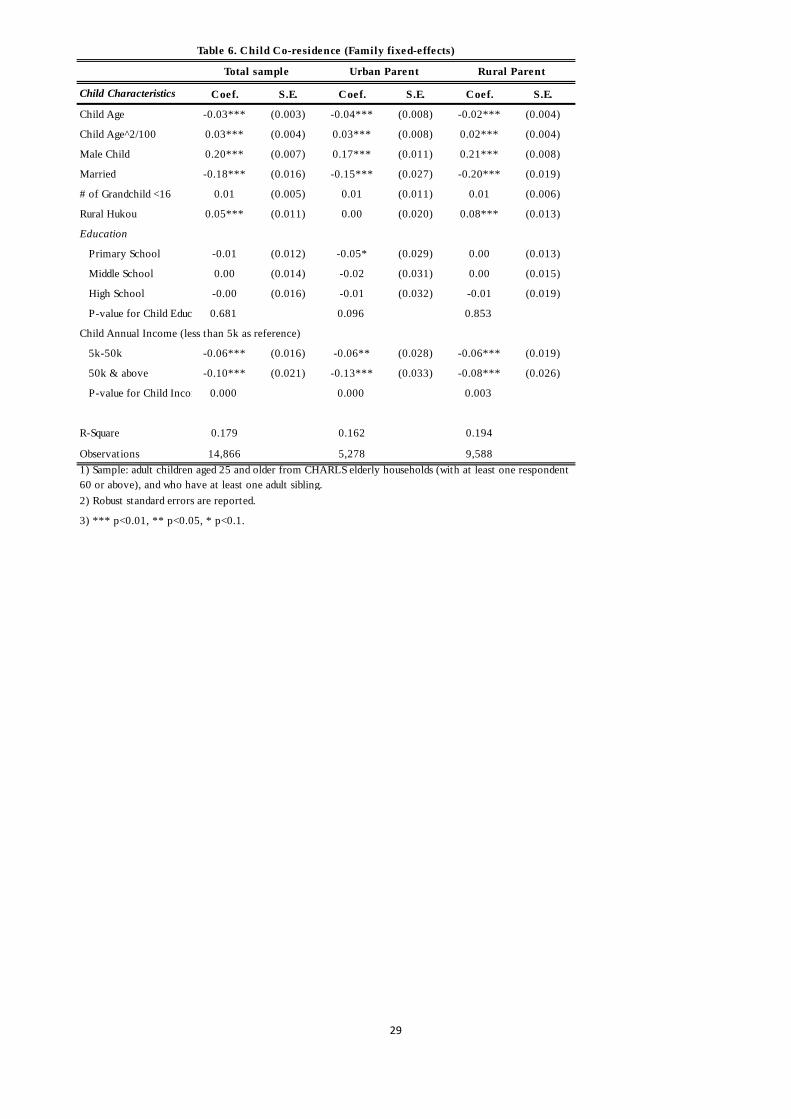
The estimates in Tables 5.1 and 5.2 may be confounded because of unobservable factors. In
Table 6, we provide an alternative model of children living with their parents, a linear probability
model which controls for family fixed effects. This model allows us to examine more closely the
influence of child characteristics on co-residence, while controlling for family-level
unobservables. The sample is restricted to those children with at least one adult sibling. Results
are similar to the first column of Table 5.1. Child income remains significant and retains a
non-linear relationship. Other results are quite similar: sons are far more likely to live with their
parents than daughters, married children less likely, children with a rural hukou, more likely. We
9 We model pre-transfer income as a linear spline with knot point at the median. The coefficient on the segment above the median is the slope (not the change in slope) over that segment. We also exclude those public transfers endogenous to number of children from the calculation of income.

15
also provide results from subsamples of the children divided according to their parents’ type of
residence. The results are quite similar for parents living in urban versus rural areas. It is very rare
to see an urban parent with a child of rural hukou, so the rural hukou coefficient for children with
urban parent is not significant.
To examine responsibility sharing among children, we further restrict our sample to families
with two or more sons, and divide male children into three groups, youngest son, oldest son, and
middle sons. From Appendix Table 2 we can see that both oldest son and youngest son (compared
to middle sons) are more likely to co-reside with elderly parents, and the youngest son has even a
higher chance than the oldest son to live with their parents. Child income has a larger effect on
children with urban parents.
The above findings are consistent with the existing literature (Meng and Luo 2004; Logan et
al. 1998; McGarry and Schoeni 2000; Zimmer and Korinek 2008). We find that co-residence is
largely dependent on elderly parents’ needs. Adult children with more children (grandchildren of
the parents) are more likely to co-reside with their parents. However resources of both children
and parents play an important role as well; in general parents with more non-housing resources
are more likely to live with their children, while children with higher levels of income are less
likely to do so.
4.2. Living Arrangements, Contact and Transfers
In this section, we examine the associations between living arrangements and other forms of
parent support: frequency of visits, other communications, and financial transfers. As transfers
and contacts can only be defined clearly among non-co-resident children and their parents, we
exclude co-resident children from this estimation.10 Again the proximity of a child is defined as
living within the same county as his/her parents. The CHARLS survey asks how many times each
10 CHARLS, like most surveys, only collects contact and transfer data on non-co-resident family members.
16
non-co-resident child visits, or communicates in other forms (call, mail, email, etc.) with elderly
parents per year. Financial transfers are measured in two ways: 1) whether the child offers transfer
to his/her elderly parents and 2) the net amount of transfers to parents.
The covariates for the contact and financial transfer regressions include both parental and
individual child characteristics. As seen from Tables 7.1 and 7.2, proximity to parents has strong
positive effects on the probability of child visits and other communications, replicating the
bivariate results in Table 4. Another factor worth noting is that, the more siblings a child has, the
less likely he/she frequently visits. A male child is more likely to visit but gender is not correlated
with the likelihood to call or contact with other communications. Child income increases the
probability of communications, and having high school or greater schooling is associated with
more non-visit communications. A single male parent gets the least attention from children.
Higher parental income is associated with an increase in visits and other communications.
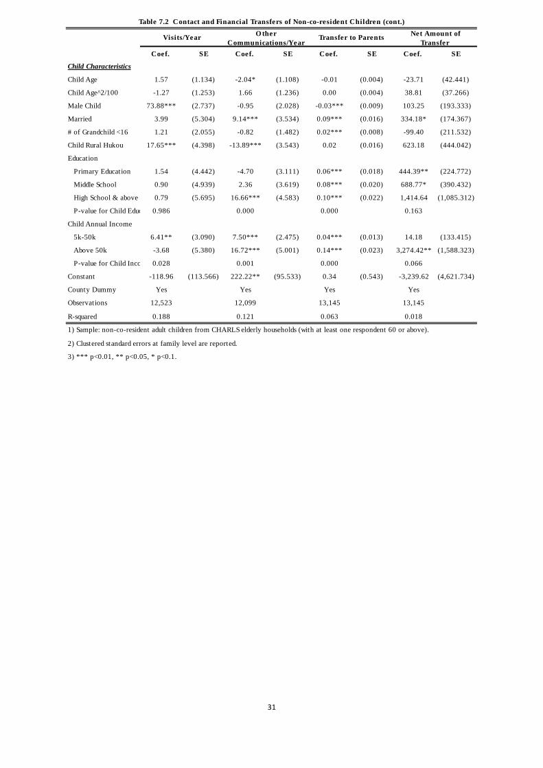
The third and fourth pairs of columns in Tables 7.1 and 7.2 report estimates on whether a
child provides transfer to his/her parents and on the net amount of transfers respectively. The
incidence of providing transfers to parents and the net amount are negatively related to proximity.
Hence those faraway children while visit less often, are more likely to make transfers and send
more money when they do make transfers. If the elderly parent co-resides with another adult child,
the non-co-resident child is less likely to provide help to parents, but the net amount is not
significantly different. The higher education the child has, the more he/she is providing to the
elderly parents and the more likely are the transfers. The same result applies to children with
higher income levels, particularly incomes above 50,000RMB per year. There is an obvious
nonlinear effect of parental pre-transfer income. A child is slightly less likely to transfer to his/her
parents if parental income is higher, but this is only true if parental income is greater than the
sample median. For parents with higher pre-transfer incomes they receive less transfers, the

17
relationship being nonlinear with a larger association for those with pre-transfer incomes below
the median.11
We also use family-fixed effects model to estimate the substitution effects between living
arrangements and other kinds of transfer. We can see from Table 8, in families with two or more
children, the results are largely the same as in Tables 7.1 and 7.2 even if we control for family
heterogeneity. However, now the associations between the size of net transfers and child
schooling and income are no longer significant, although they are with the probability of making a
transfer.
5. Conclusions
Previous literature has provided evidence that the Chinese elderly are increasingly more
likely to live alone or with a spouse only. This has raised concerns regarding support for the
elderly, considering the current lack of a strong public social security system in China. This paper
adds, using a nationally representative sample, to the growing literature that living close to parents
has become an important way of providing elderly support while at the same time maintaining
independence/privacy of both parents and children. We conclude from the results that living alone
is inadequate in describing the living arrangement of the elderly.
We also find the existence of responsibility sharing among siblings. Children who live close
to their parents more frequently visit them, providing non-financial transfers, while those living
faraway provide larger amount of financial transfers.
Investigating the determinants of elderly living arrangements and transfers we find evidence
that parents with higher pre-transfer income are more likely to live with or near their adult
children, but they tend to receive smaller amount of financial transfers from their children This
11 Cai et al. (2006), using an urban survey from China, also find less transfers as parental income rises, and also find a concave relationship, stronger for lower income parents.

18
indicates that while financial transfers may be motivated by altruistic concern of children for their
parents, the reasons for living arrangement may include other objectives, such as sharing housing
or other benefits from parents.
Estimating a family fixed-effects model, we find that sons, and particularly youngest sons,
are more likely to live with their elderly parents, an interesting result different from the tradition
of depending mostly on oldest sons. Further research is needed to explore the underlying driving
force of this transition. Daughters, as expected, are less likely to live with their parents, or to
support them financially, but this effect is weaker among children with an urban parent.
One very important set of findings has to do with correlations with the number of children.
Having a parent live with one child reduces the burden on other children in terms of visiting and
the likelihood of making a financial transfer. It is also the case that our results show that investing
in educating their children more does have a payoff in terms of being more likely to receive a
financial transfer when the parent is older. As noted, it is the case that the older cohorts in this
sample have on average 3.3 children; they were not much exposed to the One Child Policy during
most of their childbearing years, although more were partially exposed to the increasingly strong
family planning policies of the 1970s. The average parent in our sample would have been born in
1942, so they would have been in their very late twenties and early 30s even during the family
programs established during the early 1970s. It may be that cohorts younger than the ones studied
here, who were exposed to the stronger family planning programs during their childbearing ages
will be more constrained in their living arrangements than these cohorts; that is to be seen. On the
other hand, if they have invested more in their children’s schooling that may offset, at least with
regards to financial transfers.

19
References:
Agree, E. M. 1993. Effects of demographic change on the living arrangements of the elderly in Brazil: 1960-1980. PhD Dissertation. Durham, NC: Duke University.
Benjamin, D., L. Brandt, and S. Rozelle. 2000. “Aging, wellbeing, and social security in rural northern China.” Population and Development Review 26: 89-116.
Bian, F., J. R. Logan, and Y. Bian. 1998. “Intergenerational relations in urban China: Proximity, contact, and help to parents.” Demography 35: 115-24.
Cai, F., J. Giles and X. Meng. 2006. “How well do children insure parents against low retirement income?: An analysis using data from urban China”, Journal of Public Economics, 90:2229-2255.
Cameron, L. 2000. “The residency decision of elderly Indonesians: A nested logit analysis.” Demography 37: 17-27.
Costa, D. L. 1998. Displacing the family. National Bureau of Economic Research. Chicago, IL: University of Chicago Press.
Doty, P. 1986. “Family care of the elderly: The role of public policy.” The Milbank Quarterly 64: 34-75.
Edmonds, E. V. and K. Mammen, D. Miller. 2005. “Rearranging the Family? Income Support and Elderly Living Arrangements in a Low-Income Country.” The Journal of Human Resources 40: 186-207.
Engelhardt, G. V. and J. Gruber. 2004. “Social security and the evolution of elderly poverty.” NBER Working Paper Series, Vol. 10466.
Giles, J. and R. Mu. 2007. “Elderly Parent Health and the Migration Decisions of Adult Children: Evidence from Rural China.” Demography 44: 265-88.
Greenfield, E. A. and D. Russell. 2010. “Identifying Living Arrangements That Heighten Risk for Loneliness in Later Life: Evidence From the US National Social Life, Health, and Aging Project.” Journal of Applied Gerontology. Published online: 10.1177/0733464810364985
Kharicha, K., S. Iliffe, S. Illiffe, S. Harari, C. Swift, G. Gillmann, and A. Stuck. 2007. “Health risk appraisal in older people 1: are older people living alone an ‘at-risk’group?” The British Journal of General Practice 57: 271-276.
Kotlikoff, L. J. and J. N. Morris. 1990. “Why don’t the elderly live with their children? A new look.” NBER Working Paper Series, Vol. 2734.
Lin, J. 1994. “Parity and Security: A Simulation Study of Old-Age Support in Rural China.” Population and Development Review 20:423-48.
Logan, J. R., F. Bian, and Y. Bian. 1998. “Tradition and change in the urban Chinese family: The case of living arrangements.” Social Forces 76: 851-82.
Martin, L. G. 1989. “Living arrangements of the elderly in Fiji, Korea, Malaysia, and the Philippines.” Demography 26: 627-43.
McGarry, K. and R. F. Schoeni. 2000. “Social security, economic growth, and the rise in elderly widows’ independence in the twentieth century.” Demography 37: 221-36.
Meng, X. and C. Luo. 2008. “What determines living arrangements of the elderly in urban China.” Pp267–286 in Inequality and Public Policy in China, Edited by B. A. Gustafsson, S. Li; and T. Sicular. Cambridge: Cambridge University Press.
Mutchier, J. E. and J. A. Burr. 1991. “A longitudinal analysis of household and nonhousehold living arrangements in later life.” Demography 28: 375-90.
Palmer, E. and Q. Deng. 2008. “What has economic transition meant for the well-being of the

20
elderly in China.” Pp182–203 in Inequality and Public Policy in China, Edited by B. A. Gustafsson, S. Li; and T. Sicular. Cambridge: Cambridge University Press.
Silverstein, M., Z. Cong and S. Li. 2006. “Intergenerational Transfers and Living Arrangements of Older People in Rural China: Consequences for Psychological Well-Being”, Journals of Gerontology, Series B, 61(5):S256-S266.
Smeeding, T. M. and P. Saunders. 1998. “How Do the Elderly in Taiwan Fare Cross-nationally?: Evidence from the Luxembourg Income Study Project.” SPRC Discussion Paper: No. 81
Sun, R. 2001. “Old age support in contemporary urban China from both parents’ and children’s perspectives.” Research on Aging. Published online: 10.1177/0733464810364985
Tomassini, C., K. Glaser, D. A. Wolf, M. I. Broese van Groenou, and E. Grundy. 2004. “Living arrangements among older people: an overview of trends in Europe and the USA.” Further release of 2001 Census data: 1324-29.
United Nations. 2011. World Population Ageing: Profiles of Ageing, 2011, Department of Economic and Social Affairs, Population Division, New York.
Victor, C., S. Scambler, J. Bond, and A. Bowling. 2000. “Being alone in later life: loneliness, social isolation and living alone.” Reviews in Clinical Gerontology 10: 407-17.
Wilson, B. 2007. “Historical evolution of assisted living in the United States, 1979 to the present.” The Gerontologist 47(supplement): 8-22.
Zeng, Y. and Z. Wang. 2003. “Dynamics of Family and Elderly Living Arrangements in China: New Lessons Learned from the 2000 census.” China Review 3: 95-119.
Zhao, Y., G. Yang, J. Strauss, J. Giles, P. Hu, Y. Hu, X. Lei, A. Park, J.P. Smith and Y. Wang. 2013. China Health and Retirement Longitudinal Study- 2011-12 National Baseline User’s Guide. China Center for Economic Research, Peking University.
Zimmer, Z. and J. Dayton. 2005. “Older adults in Sub-Saharan africa living with children and grandchildren.” Population Studies 59: 295-312.
Zimmer, Z. and K. Korinek.2008. “Does family size predict whether an older adult lives with or proximate to an adult child in the Asia-Pacific region.” Asian Population Studies 4(2): 135-159.

21
.2.2
5.3
.35
.4.4
5P
erc
en
tag
e
6 0 6 5 7 0 7 5 8 0 8 5a g e
C e n s u s 2 0 0 0 1 % p o p u la tio n s u rv e y , 2 0 0 5
S am p le : E l de r ly s am pl e ag ed 6 0 -8 5 f ro m C en s u s 2 00 0 an d 1 % p op u la tio n s urv e y, 2 0 0 5
F igu re 1 . L iv ing A lon e o r W ith a S p ou se O n ly
.3.3
5.4
.45
.5.5
5
60 65 70 75 80 85age
Living with one or more adult childLiving alone or with spouse only
Data:CHARLS 2011, bw=0.4 , wt=household weight
Figure 2. Living Arrangements of Chinese Elderly
22
0.1
.2.3
.4.5
60 65 70 75 80 85age
Living with one or more adult childLiving alone, but with adult child in the village/communityLiving alone, but with adult child in the countyLiving alone, no adult child in the county
Data:CHARLS 2011, bw=0.4, wt=household weight
Figure 3. Living Arrangements and Proximity of Children

23
OBS Total Female Male Rural Urban East Middle WestLive alone or with spouse only 2,285 47.5 45.3 50.4 45.5 49.7 58.9 47.1 35.3
Live with children-in-law but not children 128 2.3 2.6 2.0 2.9 1.6 1.6 2.1 3.2
Live with grandchildren but not children and children-in-law 407 7.6 7.6 7.5 8.5 6.5 5.4 9.3 8.3
Live with others 178 3.6 3.6 3.5 2.9 4.4 3.1 3.8 4.1
Live with one or more adult children 1,980 39.0 40.9 36.6 40.2 37.8 31.0 37.7 49.1
Do not live with adult children, but have one or more adultchildren in the same village/community
1,731 34.4 35.1 33.5 36.5 32.2 39.9 35.9 27.0
Do not live with adult chilren, but have one or more adult children in another village/community in the same county
701 14.4 13.8 15.2 12.2 16.8 15.6 15.3 12.3
Do not live with adult children, and have no child in the samecounty
303 5.4 5.0 5.9 5.9 4.8 3.9 6.6 5.9
Have no adult child 281 6.8 5.2 8.8 5.3 8.4 9.6 4.5 5.7Observations 4,978 4,978 2,789 2,188 2,986 1,992 1,649 1,586 1,743
Table 1. Living Arrangement of Elderly Households (%) Weighted
2) Rotating parents and couples in separation are excluded3) "No adult child" is defined as having no child 25 years old or above.
1) Sample: CHARLS elderly households with at least one respondent 60 or above.

24
AllLiving with at least one adult
child
Living alone but with one or more adult child in the
county
Living alone but without any adult child in the county
P-value
DemographicsMaximum Age 69.64 68.99 70.54 66.19 0.00
(0.13) (0.21) (0.18) (0.42)Single Man 0.09 0.10 0.08 0.08 0.08
(0.00) (0.01) (0.01) (0.02)Single Woman 0.23 0.27 0.20 0.13 0.00
(0.01) (0.01) (0.01) (0.03)# of Children 3.29 3.17 3.49 2.40 0.00
(0.03) (0.04) (0.03) (0.09)Urban 0.48 0.47 0.49 0.43 0.29
(0.01) (0.01) (0.01) (0.03)Maximum Education
Illiterate 0.25 0.27 0.24 0.17 0.00(0.01) (0.01) (0.01) (0.03)
Primary 0.45 0.43 0.46 0.48 0.29(0.01) (0.01) (0.01) (0.03)
Middle School & Above 0.30 0.29 0.31 0.35 0.21(0.01) (0.02) (0.01) (0.03)
Income WealthOwn any House 0.72 0.45 0.96 0.90 0.00
(0.01) (0.01) (0.00) (0.03)Household Pre-transfer Income per Capita
7981.35 7871.86 8056.96 8090.03 0.96
(1000 RMB) (289.72) (570.48) (297.45) (905.67)Health
Worse SRH is very Poor 0.22 0.22 0.22 0.26 0.78(0.01) (0.02) (0.01) (0.05)
Any ADL/IADL Difficulty 0.37 0.41 0.35 0.23 0.00(0.01) (0.02) (0.02) (0.05)
Observations 4,697 1,980 2,914 303
Table 2. Parent Characteristics by Living Arrangements (weighted)
1) Sample: CHARLS elderly households (with at least one respondent 60 or above and with any child aged 25 and abo2) P-values of testing whether the means are equal are provided in the last column.3) Robust standard errors in brackets.

25
All Co-resident Nearby Child Non-Nearby Child P-value
DemographicsChild Age 41.46 37.82 42.73 40.04 0.00
(0.11) (0.19) (0.13) (0.17)Daughters 0.47 0.15 0.54 0.48 0.00
(0.00) (0.01) (0.01) (0.01)Fraction Married 0.92 0.77 0.95 0.91 0.00
0.00 (0.01) 0.00 (0.01)# of Grandchild Younger than 16 1.00 1.41 0.89 1.16 0.00
(0.02) (0.04) (0.02) (0.04)Rural Hukou 0.74 0.77 0.75 0.70 0.00
(0.01) (0.01) (0.01) (0.01)Education
Illiterate 0.09 0.06 0.11 0.07 0.00(0.00) (0.01) (0.00) (0.01)
Primary Education 0.39 0.34 0.41 0.38 0.00(0.01) (0.01) (0.01) (0.01)
Middle School 0.31 0.37 0.29 0.30 0.00(0.00) (0.01) (0.01) (0.01)
High School 0.20 0.22 0.19 0.25 0.00(0.00) (0.01) (0.01) (0.01)
Child Annual IncomeLess than 5k 0.11 0.20 0.10 0.06 0.00
(0.00) (0.01) (0.00) (0.00)5k-50k 0.61 0.64 0.61 0.58 0.00
(0.01) (0.01) (0.01) (0.01)50k & above 0.07 0.05 0.06 0.12 0.00
(0.00) (0.00) (0.00) (0.01)Missing 0.22 0.11 0.23 0.24 0.00
(0.01) (0.01) (0.01) (0.01)Observations 15,418 2,273 9,999 3,146
Table 3. Children's Characteristics by Living Arrangements (weighted)
1) Sample: adult children (aged 25 or above) from CHARLS elderly households (with at least one respondent 60 or above).2) Nearby child is defined as living outside of the household but within the same county.3) Clustered standard errors at family level in brackets.4) P-values of testing whether the means are equal are provided in the last column.
26
Transfer to ParentsFraction Positive 0.30 0.28 0.37 0.00
(0.01) (0.01) (0.01)Amount if >0 2.41 1.74 4.01 0.00(1000 RMB) (0.39) (0.19) (1.24)
Transfer From ParentsFraction Positive 0.08 0.08 0.08 0.00
(0.00) (0.00) (0.01)Amount if >0 3.31 3.53 2.59 0.00(1000 RMB) (0.51) (0.61) (0.81)
Net TransferAverage Amount 1.41 0.68 3.23 0.00(1000 RMB) (0.37) (0.22) (1.16)
Contact# of Visits per Year 97.72 123.27 10.30 0.00
(1.60) (1.90) (0.97)# of other Communications per Year*
58.58 63.27 44.26 0.00
(1.38) (1.67) (1.67)Observations 13,145 9,999 3,1461) Sample: non-co-resident adult children from CHARLS elderly households (with at least one respondent 60 or above).
Table 4. Contact and Financial Transfers by Living Arrangements of Non-co-resident Children
Overall Live in the county Do not live in the county
P-value
2) Transfer amounts to parent and from parent are defined as the average amount conditional on the amount is positive.3) Net transfer is defined as the amount of transfer from child to parents minus the amount of transfer the child received from parents.4) Clustered standard errors at family level in brackets.5) P-values of testing whether the means are equal are provided in the last column.
* Other communications include email, mail, phone calls, text messages, etc.

27
Child Characteristics Relative Risk Z-score Relative Risk Z-score
Child Age 0.82*** -7.891 1.10*** 4.160
Child Age^2/100 1.19*** 6.515 0.93*** -2.731
Male Child 7.41*** 23.449 0.84*** -3.588
# of Grandchild under 16 1.08 1.290 0.94 -1.497
Married 0.37*** -9.118 2.06*** 7.999
Rural Hukou 2.64*** 7.872 1.78*** 6.258
Education
Primary School 0.91 -0.587 0.84* -1.754
Middle School 1.02 0.136 0.68*** -3.521
High School & Above 0.77 -1.347 0.51*** -5.522
P-value for Child Education 0.000 0.000
Child Annual Income
5k-50k 1.05 0.588 1.00 -0.073
50k & above 0.42*** -5.304 0.41*** -8.208
P-value for Child Income 0.000 0.000
3) *** p<0.01, ** p<0.05, * p<0.1.
Table 5.1 Multinomial Estimation on Living Arrangements by Children
In the Same Household Within the County
1) Sample: Adult children aged25 and older from CHARLS elderly households (with at least on
2) Standard errors clustered at family level

28
Relative Risk Z-score Relative Risk Z-score
Parent Characteristics
Max Age 0.94 -0.762 1.11 1.575
Max Age^2/100 1.06 1.107 0.94 -1.524
P-value for Age 0.000 0.000
Single Man 1.16 1.142 1.15 1.414
Single Woman 1.10 0.930 0.97 -0.353
# of Children 0.71*** -11.850 1.06** 2.322
Urban 1.62*** 4.028 1.33*** 2.838
Highest Education
Primary Education 0.88 -1.280 0.90 -1.386
Middle School & above 0.98 -0.147 1.02 0.199
P-value for Education 0.373 0.373
Owning House 0.16*** -18.737 0.92 -1.017
For PTI below Median 1.08 0.551 1.00 0.226
For PTI above Median 1.02** 2.413 1.01*** 3.087
P-value for Income 0.008 0.008
Poorest Health
SRH very Poor 1.01 0.083 1.05 0.368
Any ADL/IADL Difficulty 0.85 -1.240 0.92 -0.787
P-value for Health 0.771 0.771
Constant 2,581.31*** 2.839 0.01** -2.299
County Dummy Yes Yes
P-value for County Dummies 0.000 0.000
Observations 15,418 15,418
3) *** p<0.01, ** p<0.05, * p<0.1.
Table 5.2 Multinomial Estimation on Living Arrangements by Children
In the Same Household Within the County
Pre-transfer Income (1000 RMB)
1) Sample: Adult children aged25 and older from CHARLS elderly households (with at least o
2) Standard errors clustered at family level
29
Child Characteristics Coef. S.E. Coef. S.E. Coef. S.E.
Child Age -0.03*** (0.003) -0.04*** (0.008) -0.02*** (0.004)
Child Age^2/100 0.03*** (0.004) 0.03*** (0.008) 0.02*** (0.004)
Male Child 0.20*** (0.007) 0.17*** (0.011) 0.21*** (0.008)
Married -0.18*** (0.016) -0.15*** (0.027) -0.20*** (0.019)
# of Grandchild <16 0.01 (0.005) 0.01 (0.011) 0.01 (0.006)
Rural Hukou 0.05*** (0.011) 0.00 (0.020) 0.08*** (0.013)
Education
Primary School -0.01 (0.012) -0.05* (0.029) 0.00 (0.013)
Middle School 0.00 (0.014) -0.02 (0.031) 0.00 (0.015)
High School -0.00 (0.016) -0.01 (0.032) -0.01 (0.019)
P-value for Child Educ 0.681 0.096 0.853
5k-50k -0.06*** (0.016) -0.06** (0.028) -0.06*** (0.019)
50k & above -0.10*** (0.021) -0.13*** (0.033) -0.08*** (0.026)
P-value for Child Incom 0.000 0.000 0.003
R-Square 0.179 0.162 0.194
Observations 14,866 5,278 9,588
2) Robust standard errors are reported.
3) *** p<0.01, ** p<0.05, * p<0.1.
Table 6. Child Co-residence (Family fixed-effects)
Total sample Urban Parent Rural Parent
Child Annual Income (less than 5k as reference)
1) Sample: adult children aged 25 and older from CHARLS elderly households (with at least one respondent 60 or above), and who have at least one adult sibling.

30
Coef. SE Coef. SE Coef. SE Coef. SE
Live in the same county 114.21*** (2.303) 23.82*** (2.208) -0.06*** (0.013) -892.05** (418.073)
Parents live with another adult child
-1.08 (3.997) 1.42 (3.644) -0.04** (0.019) -169.51 (202.969)
Parent CharacteristicsAge 0.93 (3.255) -3.59 (2.776) 0.01 (0.015) 109.30 (119.451)
Age^2/100 -0.59 (2.211) 2.29 (1.887) -0.01 (0.010) -89.61 (86.212)
Single Man -17.40*** (5.024) -19.78*** (3.960) -0.02 (0.024) 1,132.25 (1,140.270)
Single Woman -0.64 (4.033) -1.88 (3.494) 0.01 (0.020) -290.65 (278.448)
# of Children -3.13*** (1.115) -3.61*** (0.997) 0.02*** (0.005) 198.02 (150.645)
Urban 33.02*** (3.702) 18.00*** (3.275) -0.06*** (0.017) 338.19** (139.157)
Education
Primary 3.48 (3.867) 8.03** (3.160) 0.01 (0.019) -394.04 (476.912)
Middle School 3.52 (5.180) 21.52*** (4.390) -0.01 (0.025) -224.80 (524.135)
P-value for Education 0.658 0.000 0.491 0.479
House ownership -3.64 (4.493) 10.44*** (3.835) -0.02 (0.022) 21.71 (283.401)
Pre-transfer Income (1000 RMB)
For PTI below Median -1.03 (0.636) -0.73 (0.926) -0.00 (0.004) -354.87*** (128.525)
For PTI above Median 0.47** (0.192) 1.03*** (0.197) -0.00*** (0.001) -44.67** (18.887)
P-value for Income 0.024 0.000 0.000 0.001
Health
Worse SRH very Poor -10.59* (5.453) -0.55 (4.596) -0.05* (0.027) -336.42 (205.555)
Any ADL/IADL Difficulty -6.40 (4.781) -2.23 (4.007) -0.04* (0.022) -151.49 (159.522)
P-value for Health 0.007 0.799 0.003 0.136
Table 7.1 Contact and Financial Transfers of Non-co-resident Children
Visits/YearOther
Communications/Year Transfer to Parents Net Amount of
Transfer
31
Coef. SE Coef. SE Coef. SE Coef. SE
Child Characteristics
Child Age 1.57 (1.134) -2.04* (1.108) -0.01 (0.004) -23.71 (42.441)
Child Age^2/100 -1.27 (1.253) 1.66 (1.236) 0.00 (0.004) 38.81 (37.266)
Male Child 73.88*** (2.737) -0.95 (2.028) -0.03*** (0.009) 103.25 (193.333)
Married 3.99 (5.304) 9.14*** (3.534) 0.09*** (0.016) 334.18* (174.367)
# of Grandchild <16 1.21 (2.055) -0.82 (1.482) 0.02*** (0.008) -99.40 (211.532)
Child Rural Hukou 17.65*** (4.398) -13.89*** (3.543) 0.02 (0.016) 623.18 (444.042)
Education
Primary Education 1.54 (4.442) -4.70 (3.111) 0.06*** (0.018) 444.39** (224.772)
Middle School 0.90 (4.939) 2.36 (3.619) 0.08*** (0.020) 688.77* (390.432)
High School & above 0.79 (5.695) 16.66*** (4.583) 0.10*** (0.022) 1,414.64 (1,085.312)
P-value for Child Educ 0.986 0.000 0.000 0.163
Child Annual Income
5k-50k 6.41** (3.090) 7.50*** (2.475) 0.04*** (0.013) 14.18 (133.415)
Above 50k -3.68 (5.380) 16.72*** (5.001) 0.14*** (0.023) 3,274.42** (1,588.323)
P-value for Child Inco 0.028 0.001 0.000 0.066
Constant -118.96 (113.566) 222.22** (95.533) 0.34 (0.543) -3,239.62 (4,621.734)
County Dummy Yes Yes Yes Yes
Observations 12,523 12,099 13,145 13,145
R-squared 0.188 0.121 0.063 0.018
2) Clustered standard errors at family level are reported.
3) *** p<0.01, ** p<0.05, * p<0.1.
Table 7.2 Contact and Financial Transfers of Non-co-resident Children (cont.)
Visits/Year O ther Communications/Year
Transfer to Parents Net Amount of Transfer
1) Sample: non-co-resident adult children from CHARLS elderly households (with at least one respondent 60 or above).

32
Coef. SE Coef. SE Coef. SE Coef. SEChild living in the same county
107.81*** (3.537) 20.47*** (2.491) -0.03*** (0.008) -1,173.76* (702.015)
Child Characteristics
Child Age 0.65 (1.358) -0.93 (0.732) -0.00 (0.002) -8.00 (80.054)
Child Age^2/100 -0.30 (1.475) 0.97 (0.766) 0.00 (0.002) 48.54 (49.547)
Male 77.90*** (3.090) -0.28 (1.881) -0.01 (0.006) 254.83* (151.733)
Married 1.42 (6.524) 2.29 (3.446) 0.07*** (0.013) -254.16 (430.881)
# Grandchild under 16 4.76** (2.312) 0.67 (1.322) -0.00 (0.004) -306.81 (210.448)
Rural Hukou 38.68*** (5.393) 4.80 (3.279) -0.03** (0.011) 853.20 (1,017.858)
Education
Primary School 6.33 (5.582) 0.87 (3.050) 0.02 (0.011) 1,559.21 (1,300.590)
Middle School 5.02 (6.295) 8.15** (3.621) 0.03*** (0.012) 1,823.05 (1,475.922)
High School and above -4.76 (7.250) 14.63*** (4.415) 0.06*** (0.015) 2,739.72 (2,268.929)
P-value for Child Education 0.103 0.000 0.000 0.607
Child Annual Income
5k-50k 8.17 (5.114) 7.28** (2.908) 0.03*** (0.009) 1,257.59 (991.509)
50k & above -1.16 (7.558) 8.06* (4.866) 0.10*** (0.017) 3,816.30 (3,013.228)
P-value for Child Income 0.117 0.042 0.000 0.445
Observations 11,856 11,457 12,451 12,451
R-squared 0.177 0.016 0.023 0.016
2) Robust standard errors are reported.
3) *** p<0.01, ** p<0.05, * p<0.1.
Table 8 Contact and Financial Transfers of Non-co-resident children (Family fixed effects)
Visits/Year O ther Communications/Year Transfer to Parents Net Amount of Transfer
1) Sample includes non-co-resident adult children of 25 and older who have at least one parent no younger than 60 and who have at least one adult sibling.

33
Child Characteristics Relative Risk Z-score Relative Risk Z-score Relative Risk Z-score Relative Risk Z-score
Child Age 0.82*** -5.002 1.17*** 3.974 0.79*** -6.112 1.04 1.069
Child Age^2 1.16*** 3.672 0.86*** -3.649 1.26*** 5.331 1.01 0.214
Male Child 5.40*** 13.338 1.01 0.121 11.33*** 19.303 0.78*** -3.853
# Grandchild under 16 1.07 0.522 0.88 -1.429 1.11 1.465 0.97 -0.534
Married 0.35*** -5.652 1.98*** 4.718 0.38*** -6.809 2.20*** 6.518
Rural Hukou 1.63** 2.475 1.45** 2.315 5.66*** 8.735 2.36*** 7.293
Education
Primary School 1.01 0.034 1.00 -0.019 0.81 -1.083 0.83* -1.746
Middle School 1.43 0.947 0.94 -0.231 0.80 -1.092 0.63*** -3.723
High School & above 0.94 -0.144 0.63* -1.717 0.68* -1.658 0.50*** -4.542
P-value for Child Education 0.001 0.001 0.000 0.000
Child Annual Income
5k-50k 1.28* 1.701 1.13 1.115 0.93 -0.620 0.96 -0.456
50k & above 0.39*** -4.048 0.45*** -4.866 0.46*** -3.295 0.37*** -6.264
P-value for Child Income 0.000 0.000 0.000 0.000
Parent Characteristics
Age 1.00 -0.023 1.22* 1.881 0.96 -0.338 1.08 0.853
Age^2 1.03 0.278 0.88* -1.859 1.04 0.609 0.95 -0.797
P-value for Age 0.008 0.008 0.004 0.004
Single Man 2.01** 2.263 1.88** 2.389 0.91 -0.655 0.95 -0.515
Single Woman 1.44** 2.096 1.02 0.168 0.94 -0.453 0.93 -0.715
# of Children 0.69*** -7.235 1.07 1.618 0.71*** -9.701 1.06** 1.962
Education
Primary Education 0.93 -0.358 0.85 -0.942 0.86 -1.235 0.89 -1.199
Middle School& above 1.01 0.040 1.06 0.316 0.96 -0.213 0.91 -0.726
P-value for Education 0.400 0.400 0.676 0.676
Owning House 0.23*** -9.639 1.41** 2.378 0.14*** -16.787 0.78*** -2.646
Pre-transfer Income (1000 RMB)
For PTI below Median 1.35*** 3.505 0.99 -0.141 1.02 0.358 1.01 0.443
For PTI above Median 0.99 -0.736 1.00 0.962 1.06*** 3.868 1.02** 2.403
P-value for Income 0.000 0.000 0.001 0.001
Health
Worse SRH is poor 0.57** -2.036 0.65* -1.823 1.26 1.301 1.14 0.904
Any ADL/IADL Difficulty 1.24 0.803 1.04 0.168 0.80 -1.368 0.89 -0.939
P-value for Health 0.272 0.272 0.539 0.539
Constant 612.35 1.373 0.00*** -2.775 7,090.85** 2.345 0.17 -0.578
County Dummy Yes Yes Yes Yes
P-value for County Dummies 0.000 0.000 0.000 0.000
Observations 5,579 5,579 9,839 9,839
1) Sample includes adult children aged 25 and older who have at least one parent no younger than 60.
2) Standard errors clustered at family level
3) *** p<0.01, ** p<0.05, * p<0.1.
Appendix 1. Multinomial Estimation on Living Arrangements: by Urban-Rural Parent Residence
Urban Parents Rural Parents
In the Same Household Within the County In the Same Household Within the County

34
Child Characteristics Coef. S.E. Coef. S.E. Coef. S.E.
Child Age -0.02*** (0.003) -0.03*** (0.008) -0.01*** (0.004)
Child Age^2/100 0.02*** (0.003) 0.03*** (0.008) 0.01** (0.004)
Sons (Middle Sons as Reference)
Oldest Son 0.03*** (0.011) 0.06*** (0.018) 0.02* (0.013)
Youngest Son 0.10*** (0.012) 0.12*** (0.021) 0.10*** (0.015)
Daughter -0.07*** (0.010) -0.02 (0.017) -0.09*** (0.012)
Married -0.19*** (0.018) -0.15*** (0.032) -0.21*** (0.022)
# of Grandchild <16 0.01 (0.006) 0.01 (0.014) 0.01 (0.007)
Rural Hukou 0.06*** (0.012) 0.02 (0.023) 0.09*** (0.014)
Education
Primary School 0.01 (0.013) -0.02 (0.032) 0.02 (0.015)
Middle School 0.02 (0.015) 0.01 (0.034) 0.02 (0.018)
High School 0.01 (0.018) 0.01 (0.036) 0.01 (0.021)
P-value for Child Education 0.485 0.350 0.702
Child Annual Income
5k-50k -0.05** (0.019) -0.06* (0.034) -0.04** (0.022)
50k & above -0.08*** (0.024) -0.14*** (0.041) -0.05* (0.030)
P-value for Child Income 0.002 0.002 0.104
R-Square 0.151 0.153 0.158
Observations 9,812 3,128 6,684
3) *** p<0.01, ** p<0.05, * p<0.1.
Appendix Table 2. Child Co-residence for Families With at Least 2 Sons (Family Fixed-Effects)
Total sample Urban Parent Rural Parent
1) Sample includes adult children aged 25 and older who have at least one parent no younger than 60 and the family has at least two sons2) Robust standard errors are reported.