load balancing and parallelism for the...
TRANSCRIPT

LOAD BALANCING AND PARALLELISM FOR THE INTERNET
A DISSERTATION
SUBMITTED TO THE DEPARTMENT OF COMPUTER SCIENCE
AND THE COMMITTEE ON GRADUATE STUDIES
OF STANFORD UNIVERSITY
IN PARTIAL FULFILLMENT OF THE REQUIREMENTS
FOR THE DEGREE OF
DOCTOR OF PHILOSOPHY
Sundar Iyer
July 2008

c© Copyright by Sundar Iyer 2008
All Rights Reserved
ii

I certify that I have read this dissertation and that, in my opinion, it is
fully adequate in scope and quality as a dissertation for the degree of
Doctor of Philosophy.
(Prof. Nick McKeown) Principal Adviser
I certify that I have read this dissertation and that, in my opinion, it is
fully adequate in scope and quality as a dissertation for the degree of
Doctor of Philosophy.
(Prof. Balaji Prabhakar)
I certify that I have read this dissertation and that, in my opinion, it is
fully adequate in scope and quality as a dissertation for the degree of
Doctor of Philosophy.
(Prof. Frank Kelly)
Approved for the University Committee on Graduate Studies.
iii

To
my late Grandpa,
my late Grandma,
and my “grand”Ma
&
To
A sub-culture that
values Academia
iv

Abstract
Problem: High-speed networks including the Internet backbone suffer from a well-
known problem: packets arrive on high-speed routers much faster than commodity
memory can support. On a 10 Gb/s link, packets can arrive every 32 ns, while memory
can only be accessed once every ∼50ns. By 1997, this was identified as a fundamental
problem on the horizon. As link rates increase (usually at the rate of Moore’s Law),
the performance gap widens and the problem only becomes worse. The problem is
hard because packets can arrive in any order and require unpredictable operations
to many data structures in memory. And so, like many other computing systems,
router performance is affected by the available memory technology. If we are unable
to bridge this performance gap, then —
1. We cannot create Internet routers that reliably support links >10 Gb/s.
2. Routers cannot support the needs of real-time applications such as voice, video
conferencing, multimedia, gaming, etc., that require guaranteed performance.
3. Hackers or viruses can easily exploit the memory performance loopholes in a
router and bring down the Internet.
Contributions: This thesis lays down a theoretical foundation for solving the memory
performance problem in high-speed routers. It brings under a common umbrella several
high-speed router architectures, and introduces a general principle called “constraint
sets” to analyze them. We derive fourteen fundamental, not ephemeral solutions to
the memory performance problem. These can be classified under two types — (1)
load balancing algorithms that distribute load over slower memories, and guarantee
that the memory is available when data needs to be accessed, with no exceptions
whatsoever, and (2) caching algorithms that guarantee that data is available in cache
100% of the time. The robust guarantees are surprising, but their validity is proven
analytically.
Results and Current Usage: Our results are practical — at the time of writing,
more than 6M instances of our techniques (on over 25 unique product instances)
v

will be made available annually. It is estimated that up to ∼80% of all high-speed
Ethernet switches and Enterprise routers in the Internet will use these techniques.
Our techniques are currently being designed into the next generation of 100 Gb/s
router line cards, and are also planned for deployment in Internet core routers.
Primary Consequences: The primary consequences of our results are that —
1. Routers are no longer dependent on memory speeds to achieve high performance.
2. Routers can better provide strict performance guarantees for critical future
applications (e.g., remote surgery, supercomputing, distributed orchestras).
3. The router data-path applications for which we provide solutions are safe from
malicious memory performance attacks, either now and provably, ever in future.
Secondary Consequences: We have modified the techniques in this thesis to solve
the memory performance problems for other router applications, including VOQ
buffering, storage, page allocation, and virtual memory management. The techniques
have also helped increase router memory reliability, simplify memory redundancy, and
enable hot-swappable recovery from memory failures. It has helped to reduce worst-
case memory power (by ∼25-50%) and automatically reduce average case memory and
I/O power (which can result in dramatic power reduction in networks that usually have
low utilization). They have enabled the use of complementary memory serialization
technologies, reduced pin counts on packet processing ASICs, approximately halved
the physical area to build a router line card, and made routers more affordable (e.g.,
by reducing memory cost by ∼50%, and significantly reducing ASIC and board costs).
In summary, they have led to considerable engineering, economic, and environmental
benefits.
Applicability and Caveats: Our techniques exploit the fundamental nature of
memory access, and so their applicability is not limited to networking. However,
our techniques are not a panacea. As routers become faster and more complex, we
will need to cater to the memory performance needs of an ever-increasing number of
router applications. This concern has resulted in a new area of research pertaining to
memory-aware algorithmic design.
vi

Preface
“Do you have a book on stable marriages?”, I asked her with a straight face1. It was
the first book I was told to read at Stanford, and I knew full well where I could find
it. But the moment of humor was there, waiting to be exploited. She looked at me
as only a nineteen-year-old girl could — simultaneously playfully, flabbergasted, and
unimpressed . . .
Why is it hard to build high-speed routers? Because high-speed routers are like
marriages: they are unpredictable, provide no guarantees, and become vulnerable in
adversity. Not that I’m asking you to allow a 31-year-old unmarried male to lecture
you about marriage — thankfully, this thesis makes no attempt to comment on human
marriage, a topic about which the author is clueless.
This thesis is about solving the memory performance bottlenecks in building high-
speed routers. More specifically, it is about managing and resolving the preferences
and contention for memory between packets from participating inputs and outputs in
a router.
“But no one really reads a thesis . . .”, is a lament2 one often hears in academia.
It’s a remark that is neither very motivating or useful for a grad student to hear. We
humans are driven by the proud notion that the work we do (e.g., writing a thesis)
has a point. I would like to challenge the notion that a thesis is not intended to be
read. To that end, I have tried to structure the chapters so that they can be read
independently.
Almost all the research pertaining to this thesis was done in the High Performance
Network Group at Stanford University. The thesis was then written over ten months
from October 2007 to July 2008, and is now being completed after four years of
development and deployment of some of the academic ideas expounded herein (initially
at Nemo Systems, and currently in the Network Memory Group at Cisco Systems).
1Mathematical and Computer Sciences Library, Stanford University. See Chapter 4 for itsapplication to networking.
2“: : : If the work is interesting, they can always read your papers”.
vii

My industry experience benefitted me tremendously, by giving me a sense of what
is practical. Working in industry before finishing my thesis helped me ground my
ideas in reality. It also enabled me to write from an insider’s perspective, which I hope
to convey to you, the reader. While aging four years hasn’t made me any faster, I
believe it may have improved the quality of the writing — you be the judge.
If you should find typos or errors of fact, please contact me: [email protected].
Oh, and if you find mistakes in the proofs — you know what to do . . . “Mum’s the
word!” I hope that you will enjoy your reading, and that you’ll take away something
of value. So long, and thanks for all the pisces . . .
— Stanford, CA
July 2008
viii

Acknowledgements
“You have to thank some people all the time,
and all people some of the time”.
— Quick Quotations Corporation
Nick — the above quote was created for you! I am deeply indebted to you for
being a great mentor, a stellar advisor, and most important, a caring and trusted
friend. I would like to thank you for giving me your collegial respect, for guiding me
in identifying important problems, bringing out my best, and giving me the latitude
to be an independent researcher. You have inspired me in many ways, and I have
learned from your attention to detail, your focus on quality of research and writing,
and your ability to tackle big problems.
Balaji — I want to thank you for our many positive interactions, and for your
guidance, support, and deep insight into problems. I cherish and am in awe of your
mathematical abilities. Sunil, Mark, Frank, and Rajeev — thank you for being on my
dissertation and reading committee, and for your quality comments and feedback over
time.
The work on buffered crossbars and statistics counters was done with two colleagues
of whom I have always been in awe — Da and Devavrat. Amr, Rui, and Ramana, it
has been a pleasure to work with you on some aspects of this thesis. I have met some
extremely versatile people at Stanford — Martin, is there anything you do not do?
Also Guido, Pankaj, Neda, Rong, Isaac, Nandita, Pablo, Youngmi, Gireesh, Greg, and
Yashar, as well as members of the Stanford HPNG and ISN groups. It may be a given
that you are smart, but you are also humble, genuine, and wonderful human beings,
and that’s what has made you interesting to me.
It takes time to churn out a thesis, and the research of course occasionally entails
inadvertent mistakes. I would like to thank the many reviewers of my work, especially
Isaac Keslassy and Bruce Hajek, for pointing out errors in a constructive manner,
thereby helping me improve my work. I would also like to acknowledge the many
readers who helped refine the thesis, in particular Morgan, Rong, Tarun, Da, Guido,
Mainak, Pankaj, Urshit, Deb, Shadab and Andrew. Special thanks to Angshuman
for painstakingly and rigorously checking the proofs; George Beinhorn for playing
ix

Strunk and White; Henrique for helping with an early LaTeX draft; and to the many
picturesque towns of northern California where I traveled to write my thesis. I am
grateful for the fellowships provided by Cisco and Siebel Systems, and grants by the
NSF, ITRI, and Sloan Foundation.
A number of people helped make this thesis relevant to industry and helped
make its deployment a success. They include the investors at Nemo Systems and
my colleagues at Nemo and the Network Memory Group at Cisco Systems. I reserve
special thanks for Tom Edsall, Ramesh Sivakolundu, Flavio Bonomi, and Charlie
Giancarlo, for taking a keen interest and helping champion this technology at Cisco.
Last but not the least, I would like to credit Da (“colleague extraordinaire”) for being
the main force behind the delivery of these ideas. I am in awe of your sharp mind,
your ability to multitask, and your untiring efforts. Without you, these ideas would
never have reached their true potential.
Special thanks to Stanford University, for giving me the opportunity to interact
with some extraordinary and talented people from all over the world. Finally, I would
like to thank close friends who overlapped my IIT and Stanford experience — Kartik,
Kamakshi, Urshit, and Manoj, and the extended network of mentors and friends (see
Facebook!) who have given me many wonderful, meaningful, creative and of course,
hilarious moments.
I would never have made it to Stanford without the efforts of my many inspiring
professors at IIT Bombay, plus the backing of Ajit Shelat and SwitchOn Networks,
and Prof. Bhopardikar, who nurtured my love of math.
This journey would not be possible without the efforts of an amazing woman, a.k.a.
Mom, and my late grandparents. I also want to cherish Ajit for his inspirational views
and deep love of academia even as a seven-year-old, and my extended family for their
unconditional love and support in hard times. I miss you a lot. Finally, important
and too easily forgotten, I would like to acknowledge the subculture that I grew up in
during my childhood in India, which inculcates and gives tremendous (if sometimes
naıve) value to academic and creative pursuits. “Look, Ma, I . . . ”
x

Contents
Abstract v
Preface vii
Acknowledgements ix
1 Introduction 1
I Load Balancing and Caching for Router Architecture 34
2 Analyzing Routers with Parallel Slower Memories 37
3 Analyzing Routers with Distributed Slower Memories 62
4 Analyzing CIOQ Routers with Localized Memories 85
5 Analyzing Buered CIOQ Routers with Localized Memories 117
6 Analyzing Parallel Routers with Slower Memories 138
II Load Balancing and Caching for Router Line Cards 172
Part II: A Note to the Reader 173
7 Designing Packet Buers from Slower Memories 177
8 Designing Packet Schedulers from Slower Memories 221
9 Designing Statistics Counters from Slower Memories 259
10 Maintaining State with Slower Memories 280
11 Conclusions 301
Epilogue 310
xi

III Appendices & Bibliography 312
A Memory Terminology 313
B Denitions and Trac Models 317
C Proofs for Chapter 3 320
D Proofs for Chapter 5 323
E A Modied Buered Crossbar 332
F Proofs for Chapter 6 334
G Centralized Parallel Packet Switch Algorithm 340
H Proofs for Chapter 7 344
I Proofs for Chapter 9 356
J Parallel Packet Copies for Multicast 358
List of Figures 369
List of Tables 371
List of Theorems 372
List of Algorithms 376
List of Examples 377
References 379
End Notes 395
List of Common Symbols and Abbreviations 397
Index 401
xii

Chapter 1: IntroductionNov 2007, Mendocino, CA
Contents
1.1 Analogy . . . . . . . . . . . . . . . . . . . . . . . . . . . . . . . . . . . 1
1.2 Goal . . . . . . . . . . . . . . . . . . . . . . . . . . . . . . . . . . . . . 2
1.3 Background . . . . . . . . . . . . . . . . . . . . . . . . . . . . . . . . . 3
1.3.1 The Ideal Router . . . . . . . . . . . . . . . . . . . . . . . . . . . . . . 3
1.3.2 Why is it Hard to Build a High-speed Ideal Router? . . . . . . . . . . 5
1.3.3 Why is Memory Access Time a Hard Problem? . . . . . . . . . . . . . 7
1.3.4 Historical Solutions to Alleviate the Memory Access Time Problem . . 9
1.4 Mandating Deterministic Guarantees for High-Speed Routers . . 12
1.4.1 Work Conservation to Minimize Average Packet Delay . . . . . . . . . 13
1.4.2 Delay Guarantees to Bound Worst-Case Packet Delay . . . . . . . . . 13
1.5 Approach . . . . . . . . . . . . . . . . . . . . . . . . . . . . . . . . . . 16
1.5.1 Analyze Many Different Routers that Have Parallelism . . . . . . . . . 16
1.5.2 Load-Balancing Algorithms . . . . . . . . . . . . . . . . . . . . . . . . 17
1.5.3 Caching Algorithms . . . . . . . . . . . . . . . . . . . . . . . . . . . . 18
1.5.4 Use Emulation to Mandate that Our Routers Behave Like Ideal Routers 19
1.5.5 Use Memory as a Basis for Comparison . . . . . . . . . . . . . . . . . 20
1.6 Scope of Thesis . . . . . . . . . . . . . . . . . . . . . . . . . . . . . . . 21
1.7 Organization . . . . . . . . . . . . . . . . . . . . . . . . . . . . . . . . 23
1.8 Application of Techniques . . . . . . . . . . . . . . . . . . . . . . . . 27
1.9 Industry Impact . . . . . . . . . . . . . . . . . . . . . . . . . . . . . . 28
1.9.1 Consequences . . . . . . . . . . . . . . . . . . . . . . . . . . . . . . . . 29
1.9.2 Current Usage . . . . . . . . . . . . . . . . . . . . . . . . . . . . . . . 30
1.10 Primary Consequences . . . . . . . . . . . . . . . . . . . . . . . . . . 30
1.11 Summary of Results . . . . . . . . . . . . . . . . . . . . . . . . . . . . 31

A Note to the Reader
The Naga Jolokia, a chili pepper with a Scoville rating of 1 million units that grows in northeastern
India, Sri Lanka, and Bangladesh, is the hottest chili in the world, as confirmed by the Guinness World
Records [1]. To understand just how hot it is, consider that to cool its blow torch-like flame, you would
have to dilute it in sugar water over a million times!3 A milder way to put your taste buds to the test would
be to stop by an Indian, Chinese, or Thai restaurant and order a hot soup. However, your request would
be ambiguous; the context isn’t helpful, and you might confuse the waiter — that’s because the English
language, among its many nuances and oddities, doesn’t have unique terms to distinguish “temperature
hot” and “spicy-hot”.
Fortunately or unfortunately (depending on your perspective), high-speed routers offer no such
confusion. They are definitely hot (and we are not referring to the colloquial use of the term by
undergrads). They consume tremendous power — sometimes more than 5000 watts! — and dissipate
that energy as heat. This means that packet processing ASICs on these high-speed routers are routinely
built to withstand temperatures as high as 115C— temperatures so high that even the smallest contact
can blister your skin. And so, if you want to understand the workings of a high-speed router, I do not
recommend that you touch it. Instead, here are some guidelines that I believe will help make your study
of high-speed routers pleasant and safe.
• Introduction: The introductory chapter is written in a self-contained manner,
with terms defined inline. It defines the general background and motivation for
solving the memory access time problem for high-speed routers. Appendix A
has a short tutorial on memory technology.
• Independent Chapters: The chapters in this thesis are written so that, for
most part, they can be read independently. Section dependencies and additional
readings are listed at the beginning of each chapter.
• Organization: Examples and Observations are categorized separately. The
key idea in each chapter is specified in an idea box. Gray-shaded boxes contain
supplementary information. A summary is available at the end of each chapter,
and an index is provided at the end of the thesis.
3In comparison, a standard pepper spray (shame on you!) may register just over 2 million units— mighty hot, yet quickly neutralized in flowing water.

“You are rewarding a teacher poorly
if you remain always a pupil”.
— Friedrich Nietzsche† 1Introduction
1.1 Analogy
Guru: Consider a set of pigeon holes, each of which is capable of holding several
pigeons. Up to N pigeons may arrive simultaneously, and each pigeon must have
immediate access to a pigeon hole. In the same interval in which the pigeons
arrive, up to N pigeons must leave their holes. How many pigeon holes are
required to guarantee that the departing pigeons can leave their holes, and that
the arriving pigeons can enter a hole?
Shisya1: It would require just one pigeon hole with an entrance sufficiently wide to
allow N pigeons to arrive and N pigeons to depart simultaneously.
Guru: That is the ideal. But what if no pigeon hole has an entrance sufficiently wide?
Shisya: In that case, I would create N pigeon holes. Each arriving pigeon would be
directed to a separate pigeon hole. At any time, each pigeon hole must be wide
enough to receive one pigeon and allow up to N pigeons to depart.
Guru: Suppose I constrain the pigeon hole so that at any time it can either allow at
most one pigeon to arrive, or allow at most one pigeon to depart? Furthermore,
no pigeon may enter a pigeon hole while another is departing . . .
†Friedrich Nietzsche (1844-1900), German Philosopher.1Sanskrit: “student”.
1

1.2 Goal 2
The question posed in the imaginary conversation is directly applicable to the
design of Internet routers. The analogy is that an Internet router receives N arriving
packets (pigeons) in a time slot, one packet from each of its N inputs. Each packet can
be written and stored temporarily in one of several memories (analogous to pigeons
arriving in a pigeon hole). Packets can later be read from a memory (pigeons departing
from a hole). No more than N packets (destined to each of N outputs) can depart
the router during any time slot.
In defining the problem in this manner, we make several assumptions and overlook
some potential constraints. For example, (1) the available memory may in fact be
several times slower than the rate at which packets arrive, (2) the memory may not
be able to hold many packets, (3) the interconnect used to access the memories may
not support the inputs (outputs) writing to (reading from) any arbitrary combination
of memories at the same time, (4) when a packet arrives, its time of future departure
may be unknown.
We can infer from the above dialogue that if the memory was faster, or if the
packets arrived and departed at a slower rate, or if there were fewer constraints, it
would be easier to ensure that packets can leave when they need to. We will see that
the answer to the question in the conversation is fundamental to our understanding of
the design of high-speed Internet routers.
1.2 Goal
Our goal in this thesis is to design high-speed Internet routers for which we can say
something predictable and deterministic (we will formalize this shortly) regarding
their performance. There are four primary reasons for doing this:
1. Internet end-users are concerned primarily about the performance of their
applications and their individual packets.
2. Suites of applications (such as VoIP, videoconferencing, remote login, Netmeet-
ing, and storage networking) are very sensitive to delay, jitter, and packet

1.3 Background 3
drop characteristics, and do not tolerate non-deterministic performance (e.g.,
unpredictable delays) very well.
3. Hackers or viruses can easily exploit non-deterministic and known deficiencies in
router performance and run traffic-adversarial patterns to bring down routers
and the Internet.
4. If the individual routers that form the underlying infrastructure of the Internet
can be made to deliver deterministic guarantees, we can hope to say something
deterministic about the performance of the network as a whole. The network
would then potentially be able to provision for different classes of applications,
cater to delay-sensitive traffic (e.g., voice, Netmeeting, etc.), and provide end-to-
end guarantees (e.g., bandwidth, delay, etc.) when necessary.
In addition there are various secondary reasons why we want deterministic perfor-
mance guarantees from our high-speed routers. For example, unlike computer systems,
where occasional performance loss is acceptable and even unavoidable (e.g., due to
cache or page misses) router designers do not like non-deterministic performance in
their ASICs. This is because they cause instantaneous stalls in their deep pipelines, as
well as loss of performance and eventually even unacceptable packet loss. Also, many
routers are compared in “bake-off” tests for their ability to withstand and provide
guaranteed performance under even worst-case traffic conditions.
1.3 Background
1.3.1 The Ideal Router
Which factors prevent us from building an ideal router that can give deterministic
performance guarantees? Consider a router with N input and N output ports. We
will denote R (usually denoted in Gb/s) to be the rate at which packets2 arrive at
every input and depart from every output. We normalize time to the arrival time
2Although packets arriving to the router may have variable length, for the purposes of this thesiswe will assume that they are segmented and processed internally as fixed-length “cells” of size C. Thisis common practice in high-performance routers – variable-length packets are segmented into cells asthey arrive, carried across the router as cells, and reassembled back into packets before they depart.

1.3 Background 4
Line card #1
Line card #2 Line card #2
Line card #1Switch Fabric
(N writes, N reads)
R
R
R
R
2NR
Line card #8 Line card #8
R R2NR
.. ..
. . ..
Memory Card
No Buffer No Buffer
Figure 1.1: The architecture of a centralized shared memory router. The total memorybandwidth and interconnect bandwidth are 2NR.
between cells (C/R) at any input, and refer to it as a time slot.3 Assume that a single
shared memory can store all N arriving packets and service N departing packets.
This architecture is called the centralized shared memory router, and an example
with N = 8 ports and R = 10 Gb/s (these numbers are typical of mid-range routers
typically deployed by smaller local Internet Service Providers) is shown in Figure 1.1.
The shared memory router would need a memory that would meet the following
requirements:
1. Bandwidth: The memory would need to store all N packets arriving to it and
allow up to N packets to depart from it simultaneously, requiring a total memory
bandwidth of 2NR Gb/s.
2. Access Time: If we assume that arriving packets are split into fixed-size cells of
size C, then the memory would have to be accessed every At = C/2NR seconds.
3In later chapters we will re-define this term as necessary so as to normalize time for the routerarchitecture under consideration.

1.3 Background 5
For example, if C = 64 bytes, the memory would need to be accessed4 every
3.2 ns.5
3. Capacity: Routers with faster line rates require a large shared memory. As a
rule of thumb, the buffers in a router are sized to hold approximately RTT × Rbits of data during times of congestion (where RTT is the round-trip time for
flows passing through the router6), for those occasions when the router is the
bottleneck for TCP flows passing through it. If we assume an Internet RTT
of approximately 0.25 seconds, a 10 Gb/s interface requires 2.5 Gb of memory.
With 8 ports, we would need to buffer up to 20 Gb.
If the memory meets these three requirements, and the switching interconnect has
a bandwidth of 2NR to transport all N arriving packets and all N departing packets
from (to) the central memory, then the packets face no constraints whatever on how
and when they arrive and depart; and the router has minimum delay. Also, the memory
is shared across all ports of the router, minimizing the amount of memory required
for congestion buffering. This router behaves ideally and is capable of delivering the
predictable performance that we need.
1.3.2 Why is it Hard to Build a High-speed Ideal Router?
What happens if we design this high-speed ideal router using available memory
technology? Of course, we will need to use commodity memory technology. By a
commodity part, we mean a device that does not stress the frontiers of technology, is
widely used, is (ideally) available from a number of suppliers, and has the economic
benefits of large demand and supply.7 Two main memory technologies are available in
4This is referred to in the memory industry as the random cycle time, TRC .5The memory bandwidth is the ratio of the width of the memory access and the random access
time. For example, a 32-bit-wide memory with 50 ns random access time has a memory bandwidthof 640 Mb/s.
6The word router in this thesis also refers to Ethernet, ATM, and Frame Relay “switches”. Weuse these words interchangeably.
7In reality there is a fifth requirement. Many high-speed routers have product cycles that lastfive or more years, so router vendors require that the supply of these memories is assured for longperiods.

1.3 Background 6
the market today: SRAM and DRAM. Both offer comparable memory bandwidth;
however, SRAMs offer lower (faster) access time, but lower capacity than DRAMs.
Example 1.1. At the time of writing, with today’s CMOS technology, the largest
available commodity SRAM [2] is approximately 72 Mbits, has a band-
width of 72 Gb/s, an access time of 2 ns, and costs $70.8
To meet the capacity requirement, our router would need more than 275 SRAMs,
and the memories alone would cost over $19K – greatly exceeding the selling price of
an Enterprise router today! Although possible, the cost would make this approach
impractical.
Example 1.2. The largest commodity DRAM [3] available today has a capacity of
1Gb, a bandwidth of 36 Gb/s, an access time of 50 ns, and costs $5.
We cannot use DRAMs because the access rate9 is an order of magnitude above
what is required. If our router has more than N = 16 ports, the access time requirement
would make even the fastest SRAMs inapplicable.
The centralized shared memory router is an example of a class of routers called
output queued (OQ) routers. In an OQ router (as shown in Figure 1.2), arriving
packets are placed immediately in queues at the output, where they contend with
other packets destined to the same output. Since packets from different outputs do
not contend with each other, OQ routers minimize delay and behave ideally. An OQ
router can have N memories, one memory per output. Each memory must be able to
simultaneously accept (write) N new cells (one potentially from every input) and read
one cell per time slot. Thus, the memory must have an access rate proportional to
N +1 times the line rate. While this approximately halves the access time requirement
compared to the centralized shared memory router, this approach is still extremely
impractical at high speeds.
8As noted above, this does not preclude the existence of higher-speed and/or larger-capacitySRAMs, which are not as yet commodity parts.
9The access rate of a memory is the inverse of the access time, and is the number of times that amemory can be uniquely accessed in a time slot.

1.3 Background 7
(N+1)R
Line card #1
Line card #2 Line card #2
Line card #1
R
R
Line card #8 Line card #8
R
..
NR
Switch Fabric
R
R
R
..
(N+1)R..
(N+1)R..
. .
(N writes, 1 read) (No Buffer)
Figure 1.2: The architecture of an output queued router. The memory bandwidth on anyindividual memory is (N + 1)R.
In summary, although OQ routers are ideal and have attractive performance, they
are not scalable due to the memory access time limitations.
1.3.3 Why is Memory Access Time a Hard Problem?
If memory bandwidth or capacity were a problem, we could simply using more memories
in parallel! For example, many Ethernet and Enterprise line cards [4]10 use up to 8
memories in parallel to meet the bandwidth requirements. Similarly, the CRS-1 [5]
core router, one of the highest-speed Internet routers available today, uses up to 32
memories to meet its large buffer capacity requirement. While this approach has its
limits (having a large number of memories on a line card is unwieldy, and the number
of parts that can be used in parallel is limited by the die area of the chips, board size,
and cost constraints), it offers a simple way to achieve higher memory capacity and
bandwidth.
NObservation 1.1. However, memory access time is a more fundamental limitation.
While packets can easily be spread and written over multiple parallel
10For simplicity, we will use the terms line card and port interchangeably, and assume that a linecard terminates exactly one port. In reality, a line card can receive traffic from many ports.

1.3 Background 8
memories, it is difficult to predict how the data will be read out later. If
we want to read from our memory subsystem, say, every 3.2 ns, and all
the consecutive packets reside in a DRAM with a much slower access
time, then having other parallel memories won’t help.
Although the access time11 will be reduced over time, the rate of improvement
is much slower than Moore’s Law [6]. Note that even newer DRAMs with fast I/O
pins – such as DDR, DDRII, and Rambus DRAMS [7] – have very similar access
times. While the I/O pins are faster for transferring large blocks, the access time to a
random location in memory is still approximately 50 ns. This is because high-volume
DRAMs are designed for the computer industry, which favors capacity over access time.
Also, the access time of a DRAM is determined by the physical dimensions of the
memory array (and therefore line capacitance), which stays constant from generation
to generation.
Commercial DRAM manufacturers have recently developed fast DRAMs (RL-
DRAM [8] and FCRAM [9]) for the networking industry. These reduce the physical
dimensions of each array by breaking the memory into several banks. This worked
well for 10 Gb/s line rates, as it meant these fast DRAMs with 20 ns access times
could be used. But this approach has a limited future, for two reasons: (1) as the
line rate increases, the memory must split into more and more banks, which leads to
an unacceptable overhead per bank,12 and (2) even though all Ethernet switches and
Internet routers have packet buffers, the total number of memory devices needed is a
small fraction of the total DRAM market, making it unlikely that commercial DRAM
manufacturers will continue to supply them.13
NObservation 1.2. Fundamentally, the problem is that networking requires extremely
small-size data accesses, equal to the size of the smallest-size 64-byte
11The random access time should not be confused with memory latency, which is the time takento receive data back after it has been issued by the requester.
12For this reason, the third-generation parts are planned to have a 20 ns access time, just like thesecond generation.
13At the time of writing, there is only one publicly announced source for future RLDRAM devices,and no manufacturers for future FCRAMs.

1.3 Background 9
packet. By 1997, this was identified as a fundamental upcoming
problem.
As line rates increase (usually at the rate of Moore’s Law), the time it takes
these small packets to arrive grows linearly smaller. In contrast, the random access
time of commercial DRAMs has decreased by only 1.1 times every 18 months (slower
than Moore’s Law) [10]. And so the problem only becomes harder. If we want to
design high-speed routers whose capacity can scale, and that can give predictable
performance, then we need to alleviate the memory access time problem.
NObservation 1.3. By 2005, routers had to be built to support the next-generation
40 Gb/s line cards. By then, this had become a pressing problem in
immediate need of a solution.
1.3.4 Historical Solutions to Alleviate the Memory Access
Time Problem
Since the first routers were introduced, the capacity of commercial routers14 has
increased by about 2.2 times every 18 months (slightly faster than Moore’s Law). By
the mid-1990s, router capacity had grown to the point where the centralized shared
memory architecture (or output queuing) could no longer be used, and it became
popular to use input queueing instead.
In an input queued router, arriving packets are buffered in the arriving line cards
as shown in Figure 1.3(a). The line cards were connected to a non-blocking crossbar
switch which was configured by a centralized scheduling algorithm. From a practical
point of view, input queueing allows the memory to be distributed to each line card,
where it can be added incrementally. The switching interconnect needs to carry up
to N packets from the inputs to the respective outputs and needs a bandwidth of
14We define the capacity of a router to be the sum of the maximum data rates of its line cards, NR.For example, we will say that a router with 16 OC192c line cards has a capacity of approximately160 Gb/s.

1.3 Background 10
Line card #1
Line card #2 Line card #2
Line card #1
R
R
Line card #8 Line card #8
R
. . ..
2R
Switch Fabric
2R
2R
R
R
RNR
No Buffer 1 Write, 1 Read
(a) Input Queued Router
Line card #1
Line card #2 Line card #2
Line card #1
R
R
Line card #8 Line card #8
R
. . ..
Switch Fabric
R
R
R2NR
2 Writes, 1 Read 1 Write, 2 Reads . .
3R
3R
3R
3R3R
3R
(b) CIOQ Router
Figure 1.3: The input-queued and CIOQ router architectures.
2NR. More important, each memory only needs to run at a rate 2R (instead of 2NR),
enabling higher-capacity routers to be built.
A router is said to give 100% throughput if it is able to fully utilize its output
links.15 Theoretical results have showed that with a queueing structure called virtual
output queues (VOQs), and a maximum weight matching scheduling algorithm, an
input queued router can achieve 100% throughput [11, 12]. However, in an input
queued router, it is known that a cell can be held at an input queue even though its
output is idle. This can happen for an indefinitely long time. So there are known
simple traffic patterns [13] that show that an input queued router cannot behave
identically to an OQ router.
Another popular router architecture is the combined input-output queued (CIOQ)
router, shown in Figure 1.3(b). A CIOQ router buffers packets twice – once at the input,
and again at the output. This router can behave identically16 to an output queued
router if the memory on each line card runs at rate 3R, the switching interconnect
runs at rate 2NR, and it implements a complex scheduling algorithm [13].
Table 1.1 summarizes some well-known results for the above router architectures.
While the results in Table 1.1 may appeal to the router architect, the algorithms
15For a formal definition, see Appendix B.16We define this formally later and refer to it as emulate.

1.3 Background 11
required by the theoretical results are not practical at high speed because of the
complexity of the scheduling algorithms. For these reasons, the theoretical results
have not made much difference in the way routers are built. Instead, most routers
use a heuristic scheduling algorithm such as iSLIP [14] or WFA [15], and a memory
access rate between 2R and 3R.17 Performance studies are limited to simulations
that suggest most of the queueing takes place at the output, potentially allowing
it to behave similarly to an output queued router. While this may be a sensible
engineering compromise, the resulting system has unpredictable performance, cannot
give throughput guarantees, and the worst case is not known.
Other multi-stage and multi-path router architectures have been used. They
include Benes, Batcher-banyan [16], Clos, and Hypercube switch fabrics. However,
they either require large switching bandwidth, require multiple stages of buffering, or
have high communication complexity between the different stages. The implementation
complexity and hardware costs involved have restricted their popular use.
In comparison to CIOQ routers, other router architectures tend to hit their hardware
limits earlier. This affects their scalability, and so, primarily as a compromise, CIOQ
routers have emerged as a common router architecture, even though the performance
of practical CIOQ routers is difficult to predict. This is not very satisfactory, given
that CIOQ routers make up such a large fraction of the Internet infrastructure. While
the architectures described above are an improvement over OQ routers, these routers
require that the access rate of the memories is at least as fast as the line rate R. Even
an input queued router needs a memory that can be accessed at least twice (once to
read and once to write a packet) during every time slot. As line rates increase, this
may become impossible even with SRAMs.
17This refers to a “speedup” between one and two. We will avoid the use of the metric commonlycalled “speedup” in our discussion of memory. The term speedup is used differently by differentauthors; there is no accepted standard definition. Instead, we will compare different router memorysubsystems based on their memory access rate and memory bandwidth. We will, however, define“speedup” and use it as appropriate for other operations related to memory, e.g., when we refer tothe speed at which switching interconnects operate, updates are done, or copies are made.

1.4 Mandating Deterministic Guarantees for High-Speed Routers 12
Table 1.1: Comparison of router architectures.
Router Type#
mem
Mem.AccessRate.18
Total mem.BW
InterconnectBW
Comment
CentralizedShared Memory
1 ≡ Θ(2NR) 2NR 2NRIdeal Router
(Shared Memory)
Output Queued N ≡ Θ(N + 1)R N(N + 1)R NRIdeal Router
(Distributed Memory)
Input Queued N ≡ Θ(2R) 2NR NRCannot emulate an
ideal router
CIOQ 2N ≡ Θ(3R) 6NR 2NRCan emulate an ideal
router [13]
Example 1.3. For example, with the advent of the new 100Gb/s line cards, even
an input queued router would need an access time of 2.56 ns to buffer
64-byte packets. This is already out of reach of most commodity
SRAMs today.
1.4 Mandating Deterministic Guarantees for High-
Speed Routers
Our goal is to build high-speed routers than can give performance guarantees. As
we saw, building a slow-speed router with performance guarantees is easy. But the
problem is hard when designing high-speed routers. In fact, today, there are no
high-speed routers with bandwidths greater than 10 Gb/s that give deterministic
guarantees. There are typically two types of performance guarantees: statistical (the
most common example being 100% throughput) and deterministic (the most common
examples being work-conservation and delay guarantees).
Even statistical guarantees are hard to achieve. In fact, no commercial high-speed
router today can guarantee 100% throughput. If we buy a router with less than 100%
throughput, we do not know what its true capacity is. This makes it particularly hard
for network operators to plan a network and predict network performance. In normal
times (when the utilization of the network is quite low), this does not matter, but
18The Θ(·) notation is used to denote an asymptotically tight bound in the analysis of algorithms.In the context of this thesis it denotes that the actual value is within a constant multiple of the valuegiven.

1.4 Mandating Deterministic Guarantees for High-Speed Routers 13
during times of congestion (usually due to link failures), when network performance
really matters, this is unacceptable. We want to design routers that give 100%
throughput.
However, we will specifically demand that our high-speed routers give deterministic
performance guarantees on individual packets, since this will enable us to meet
the goals outlined in Section 1.2. Also, if routers give deterministic guarantees,
they automatically give statistical guarantees. We are interested in two classes of
deterministic guarantees, both of which have relevance for the end-user.
1.4.1 Work Conservation to Minimize Average Packet Delay
ℵDenition 1.1. Work-conserving: A router is said to be work-conserving if an
output will always serve a packet when a packet is destined for it in
the system.
We want our routers to be work-conserving. If a router is work-conserving, then
it has 100% throughput, because the outputs cannot carry a higher workload. It
also minimizes the expected packet delay, since, on average, packets leave earlier in a
work-conserving router than in any other router.19 To achieve work conservation, we
will use first come first served (FCFS) as the main service policy in our analysis of
routers. This means that packets to a given output depart in the order of their arrival.
However, the techniques that we use to analyze router architectures allow us to extend
our results to any work-conserving router if the departure time20 is known on arrival.
1.4.2 Delay Guarantees to Bound Worst-Case Packet Delay
A standard way that routers can provide delay guarantees is to introduce harder
constraints by shaping or streamlining the arrival traffic; for example, the leaky-bucket
19Strictly speaking, this is only true if all packets have the same size. When packets have differentsizes, a router could re-order packets based on increasing size and service the smallest packets first tominimize average delay. This is unimportant because the order of departure of packets cannot bearbitrarily changed by a router.
20The departure time for an arriving cell for an FCFS queuing service policy can be easilycalculated. It is the first time that the server (output) is free and able to send the newly arriving cell.

1.4 Mandating Deterministic Guarantees for High-Speed Routers 14
constraint.21 The constrained arriving streams are then serviced by a scheduler (such
as, say, a weighted fair queueing [17] scheduler) that provides service guarantees. There
are two ways to achieve this —
Maintaining separate FIFO queues: Every arrival stream is constrained and
stored in a separate queue. A scheduler works in round robin order by looking at
these queues and taking the head-of-line packets from the queues. The packets are
serviced in the order of their departure time22 and leave the output in that sorted
order. Figure 1.4(a) shows an example of the input traffic, A(t), constrained and split
into its three constituent streams, A(1), A(2), and A(3), and stored in their three
respective queues. The three queues are serviced by a scheduler in the ratio 2 : 1 : 1.
From well-known results on weighted fair queueing [18], it is then possible to define
bounds on the worst-case delay faced by a packet transiting the router.
Maintaining a single logical queue: Another way to do this is to move the
sorting operation into a “logical” queue known as the push-in first-out (PIFO) queue.
A PIFO queue has a number of key features:
1. Arriving packets are “pushed-in” to an arbitrary location in the departure queue,
based on their finishing time.
2. Packets depart from the head of line (HoL).
3. Once the packet is inserted, the relative ordering between packets in the queue
does not change.
Therefore, once a packet arrives to a PIFO queue, another packet that arrives later
may be pushed in before or after it, but they never actually switch places. This is
the characteristic that defines a PIFO queue. PIFO includes a number of queueing
policies, including weighted fair queueing [17] and its variants such as GPS [18], Virtual
Clock [19], and DRR [20]. It also includes strict priority queueing.23
21This is defined in Section 4.3.1.22Also referred to in literature as finishing time.23Note that some QoS scheduling algorithms such as WF2Q [21] do not use PIFO queuing.

1.4 Mandating Deterministic Guarantees for High-Speed Routers 15
A2FIFO Q1
A(t)
A1(t)
FIFO Q2
A3(t)
A2(t)
A1
FIFO Q3
A2Before: C2, B2, C1, B1, A1
After: C2, B2, C1, B1, A2, A1
A2
A(t)A1C1B2C2
PIFO Queue Before: C2, B2, C1, B1, A1
After: C2, B2, C1, B1, A2, A1
A2
B1
(a) Multiple FIFO Queues
(b) PIFO Queue
Output Port Departure Order
Output Port Departure Order
Traffic
Constrain
Traffic
Constrain
B1B2
C1C2
Figure 1.4: Achieving delay guarantees in a router. (a) Multiple FIFO queues, (b) A“logical” push in first out queue.
Example 1.4. As Figure 1.4(b) shows, the PIFO queue always maintains packets in
a sorted order. When packets come in, they are inserted in the sorted
order of their departure times. In Figure 1.4(a), arriving cell A2 is
inserted at the tail of FIFO Q1 and awaits departure after cell A1 but
before cell B1. In Figure 1.4(b), it is inserted directly into the sorted
PIFO queue after cell A1 but before cell B1.
Depending on the architecture being used, we choose either the set of logical FIFO
queues, or the sorted PIFO queue to make our analysis easier.

1.5 Approach 16
1.5 Approach
1.5.1 Analyze Many Dierent Routers that Have Parallelism
While it is difficult to predict the course of technology and the growth of the Internet,
it seems certain that in the years ahead routers will be required with: (1) increased
switching capacity, (2) support for higher line rates, and (3) support for differentiated
qualities of service. Each of these three requirements presents unique challenges. For
example, higher-capacity routers may require new architectures and new ways of
thinking about router design; higher line rates will probably exceed the capabilities of
commercially available memories (in some cases this transition has already happened),
making it impractical to buffer packets as they arrive; and the need for differentiated
qualities of service will mandate deterministic performance guarantees comparable to
the ideal router.
NObservation 1.4. There will probably be no single solution that will meet all needs.
Each router architecture will have unique tradeoffs. Very-high-speed
interconnect technologies may make certain new router architectures
possible, or possibly simplify existing ones. Memory access speeds may
continue to lag router requirements to such a degree that architectures
with memories with much slower access rates may become mandatory.
If memory capacity lags router buffer sizing requirements, architectures
with shared memory will become important.
We won’t concern ourselves with whether a particular technique is currently
implementable, nor will we prefer one router architecture over another, since the cost
and technology tradeoffs will be driven by future technology. We will also be agnostic
to trends in future technology. The only assumption we will make is that memory
access time will continue to be a bottleneck in one form or another. In order to
alleviate this bottleneck, we will consider router architectures that have parallelism.

1.5 Approach 17
Our approach is to analyze different types of parallel router architectures, work
within the technology constraints on them, and ask what it will take for these routers
to give deterministic performance guarantees. We will not attempt to analyze all
router architectures exhaustively; in fact, future technologies may lead to completely
novel architectures. Instead, we will focus on architectural and algorithmic solutions
that exploit the characteristic of memory requirements on routers, so that they can be
applied to a broad class of router architectures. We will focus on two key ideas: load
balancing and memory caching,24 that alleviate the load on memory.
1.5.2 Load-Balancing Algorithms
A load balancing algorithm is motivated by the following idea —
DIdea. “We could intelligently distribute load among parallel memories.a such
that no memory needs to be accessed faster than the rate that it can support”.
aIdeally, there will be no limit as to how slow these parallel memories can operate.
In order to realize the above idea, a load balancing algorithm usually needs to
be aware a priori of the time when a memory will be accessed. We introduce a
new mathematical technique called constraint sets which will help us analyze load
balancing algorithms for routers. We have found that memory accesses in routers are
fundamentally clashes between writers (e.g., arriving packets that need to be buffered)
and readers (e.g., packets that need to depart at a particular future time) that need
to simultaneously access a memory that cannot keep up with both requirements at
the same time. Constraint sets are a formal method to mathematically capture these
constraints. While the constraint set technique is agnostic to the specifics of the router
architecture, the actual size and definition of these sets vary from router to router.
This helps us separately analyze the load balancing algorithm constraints for each
individual router, and:
24These are standard techniques in use in the fields of distributed systems and computer architec-ture.

1.5 Approach 18
1. identify the memory access time, memory, and switching bandwidth required for
a specific router architecture to be work-conserving,
2. define a switching algorithm for the router,
3. identify the design tradeoffs between memory access time, memory bandwidth,
switch bandwidth, and switching algorithms, and
4. perhaps surprisingly, exactly characterize the cost of supporting delay guarantees
in a router.
1.5.3 Caching Algorithms
The second approach we use is building a memory hierarchy, and is motivated by the
following idea:
DIdea. “We can use a fast on-chip cache memory that can be accessed at high
rates, and a slowa off-chip main memory that can be accessed at low rates”.
aThe slow memory can potentially be off-chip and have a large memory capacity.
The idea is similar to that used in most processors and computing systems. Packets
or data that are likely to be written or read soon are held in fast cache memory, while
the rest of the data is held in slower main memory. If we have prior knowledge about
how the memory will be accessed (based on knowledge of the data structures required
to be maintained by routers), then we can (1) write data in larger blocks at a slower
access rate, and (2) pre-fetch large blocks of data from main memory at slower access
rates and keep it ready before it needs to be read.
NObservation 1.5. But unlike a computer system, where is acceptable for a cache to
have a miss rate, such behavior is unacceptable in networking, since it
can lead to loss of throughput and packet drops.
Therefore, our cache design should be able to guarantee a 100% hit rate under
all conditions. We will see that, within bounds, such caching algorithms exist for

1.5 Approach 19
certain applications that are widely used on most routers. As an example, packets are
maintained in queues; the good thing is that we know which data will be needed soon
– it’s sitting at the head of the queue. We will borrow some existing mathematical
techniques to propose and analyze caching algorithms, such as difference equations
and Lyapunov functions, which have been used extensively in queueing analysis.
1.5.4 Use Emulation to Mandate that Our Routers Behave
Like Ideal Routers
We want to ensure that any router that we design will give us deterministic performance
guarantees. We therefore compare our router to the ideal OQ router. To do this, we
assume that there exists an OQ router, called the “shadow OQ router”, with the same
number of input and output ports as our router. The ports on the shadow OQ router
receive identical input traffic and operate at the same line rate as our router. This
is shown in Figure 1.5. Consider any cell that arrives to our router. We denote DT ,
the departure time of that cell from the shadow OQ router. We say that our router
mimics [13, 22, 23] the ideal router if under identical inputs, the cells also depart our
router at time DT . If we want work conservation, we will compare our router to a
shadow OQ router performing an FCFS policy (called an FCFS-OQ router). If we
want delay guarantees, our comparison will be with a PIFO-OQ shadow router.
Note that the router we compare may have some fixed propagation delays that
we wish to ignore (perhaps the data transits a slower interconnect, or is buffered in a
slower memory, etc.). In particular, we are only interested in knowing whether our cell
faces a relative queueing delay, i.e., an increased queueing delay (if any) relative to
the delay it receives in the shadow OQ router. We are now ready to formally compare
our router with an ideal router.
ℵDenition 1.2. Emulate: A router is said to emulate an ideal shadow OQ router if
departing cells have no relative queueing delay, compared to the shadow
OQ router.

1.5 Approach 20
Line card #1
Line card #2 Line card #2
Line card #1
R
R
R
R
Line card #8 Line card #8
R R
. . ..
Any Router
Shadow OQ Router
Departure Time = DT
R
R
R
R
R
R
R
Em
ulate?
Yes?
PerformanceGuarantees
Determinsitic
Line card #1
Line card #2 Line card #2
Line card #1Switch Fabric
Memory Card
R
R
R
R
2NR
Line card #8 Line card #8
R R2NR
.. ..
. . ..
Iden
tica
l In
puts
C
C
R
C
C
Switch Fabric
Figure 1.5: Emulating an ideal output queued router.
Note that the definition of emulation makes no assumptions on the packet sizes,
the bursty nature of packet arrivals, or the destination characteristics of the packets,
and requires that the cells face no relative delay irrespective of the arrival pattern. An
important consequence of this definition is as follows — the ideal output queued router
is safe from adversarial traffic patterns (such as can be created by a hacker or virus)
that exploit potential performance bottlenecks in a router. If our router can emulate
an OQ router, then our router is also safe from adversarial performance attacks!
1.5.5 Use Memory as a Basis for Comparison
Throughout this thesis, we will use memory for comparison. We will look at architec-
tures that alleviate memory access time requirements. And we will see that doing so
requires tradeoffs on other components; for example, we may need more total memory
bandwidth, more interconnect bandwidth, an on-chip cache, etc. We believe that
memory serves as a good metric, for three reasons:

1.6 Scope of Thesis 21
1. Routers are, and will continue to be, limited by the access rate and memory
bandwidth of commercially available memories in the foreseeable future. All else
being equal, a router with smaller overall access rate and memory bandwidth
requirements can have a higher capacity.
2. Memory components alone contribute approximately 20% of the cost of materials,
on average. In certain high-speed market segments, almost a third of the cost
comes from memory [24]. Cisco Systems, the leading Internet router vendor,
alone spends roughly $800M p.a. on memory components. Routers with lower
memory bandwidth will need less memory, and will be more cost-efficient.
3. A router with higher memory bandwidth will, in general, consume more power.
Routers are frequently limited by the power that they consume (because they are
backed up by batteries) and dissipate (because they must use forced-air cooling).
The total memory bandwidth indicates the total bandwidth of the high-speed
I/Os that connect the memories to control logic. As an example, high-speed
memory I/O contributes to approximately 33% of the overall power on Ethernet
switches and Enterprise routers [25].
Similar to computing systems, memories are (and in the foreseeable future will
continue to be) the main bottleneck to scaling the capacity and meeting the cost and
power budgets of high-speed routers.
1.6 Scope of Thesis
This thesis is about the router data-plane, which processes every incoming packet,
and needs to scale with increasing line rates.25 The data-plane needs to perform
many computational tasks, such as parsing arriving packets, checking their integrity,
extracting and manipulating fields in the packet, and adding or deleting protocol
headers, as shown in Figure 1.6. In addition it performs several algorithmic tasks, such
as forwarding lookups to determine the correct packet destination, packet and flow
25We do not consider problems in the router control plane, which usually runs much slower thanline rate and is involved with management, configuration, and maintenance of the router and networkconnectivity.

1.6 Scope of Thesis 22
Switch Fabric
Centralized Switching
..
Compute/Algorithmic Memory Intensive
R
Data Plane
RParsing
Extraction
Lookups
Classification
Manipulation
State
Measurem
ents
Buffering
QoS Scheduling
Distributed Sw
itching
Router Line Cards ..
Parsing
Extraction
Lookups
Classification
Manipulation
State
Measurem
ents
Buffering
Scheduling
Switching
..
Parsing
Extraction
Lookups
Classification
Manipulation
State
Measurem
ents
Buffering
Scheduling
Switching
..
Parsing
Extraction
Lookups
Classification
Manipulation
State
Measurem
ents
Buffering
Scheduling
Switching
..
Parsing
Extraction
Lookups
Classification
Manipulation
State
Measurem
ents
Buffering
Scheduling
Switching
..
Parsing
Extraction
Lookups
Classification
Manipulation
State
Measurem
ents
Buffering
Scheduling
Switching
Switching(Arbitration)
Processor
Control Plane
Packet Copying
Tasks Tasks
Figure 1.6: The data-plane of an Internet router.
classification (e.g., for security, billing and other applications), deep packet inspection
(e.g., for virus filtering), etc. A number of algorithms and specialized hardware (such
as CAMs, hardware assisted classifiers, complex parsers, etc.) have been proposed to
make these tasks efficient. We do not address any of these computational or algorithmic
tasks in this thesis. Instead, we focus on the tasks in the router data-path for which
memory is a bottleneck, as shown in Figure 1.6.
At a minimum, a router needs to buffer and hold packets in memory during times
of congestion. It needs to switch packets across a switching fabric and move these

1.7 Organization 23
packets to their correct output line cards (where it may again be buffered temporarily).
As shown in the figure, switching can be performed centrally, or by each line card in a
distributed manner. In addition, routers perform measurements and keep statistics
in memory, for purposes of billing, metering, and policing traffic. Statistics are also
useful for planning, operating, and managing a network. Routers perform packet
scheduling as described in Section 1.4.2 to provide various qualities of service. In
some cases, specialized application-aware routers maintain state for flows to perform
complex tasks such as application proxies, network address translation, etc., as well as
maintain policing, shaping, and metering information. In some cases, routers need
to support packet multicasting, where packets may need to be copied multiple times.
As we shall see, each of the above tasks requires high memory access rates. This
thesis studies the nature of the data structures needed by the above tasks, and takes
advantage of their associated memory accesses to alleviate their memory bottlenecks.
1.7 Organization
In Section 1.3.1, we saw that an ideal output queued router requires a memory access
rate that is proportional to the product of the number of ports N and the line rate of
each port R. In the remainder of the thesis, we will look at ways to reduce the access
rate of the memory on high-speed routers. This is done by trading off memory access
time with memory bandwidth, capacity or a cache as summarized in Table 1.2. We
divide the rest of this thesis into two parts:
Part I: Load Balancing and Caching Algorithms for Router
Architecture
In the first part of the thesis, we will consider how we can scale the performance
of the router as a whole. Thus, in Chapter 2, we first define a new class of router
architectures, called “single-buffered” routers that are of particular interest. We also
answer the question posed in the conversation in the Introduction, since it sheds light
on the analysis of all single-buffered routers. Then, in each chapter, we ask a question
about the technology and the architectural constraints that the memory on a router

1.7 Organization 24
Table 1.2: Organization of thesis.
Chpt. Analysis Memory Tradeoff
1 Output Queued Router Ideal router2 Parallel Shared Mem. Router More Memory bandwidth
3-(a) Distributed Shared Mem. Router More Memory bandwidth3-(b) Parallel Distributed Shared Mem. Router More Memory bandwidth
4 CIOQ Router More Memory bandwidth5 Buffered CIOQ Router Line rate cache
6-(a) Parallel Packet Switch More Memory bandwidth6-(b) Buffered Parallel Packet Switch Line rate cache7-(a) Packet Buffer Cache Line rate cache7-(b) Pipelined Packet Buffer Cache Line rate pipelined cache
8 Packet Scheduler Cache Line rate cache9 Statistics Counter Cache Line rate cache10 Parallel Packet State More memory bandwidth, capacity
App. J Parallel Packet Copy More memory bandwidth
might face, as it pertains to its overall architecture:
Chpt. 2: What if the memories must be shared? Memory capacity could be-
come a problem, and shared memory architectures could become mandatory. In
Chapter 2, we look at a parallel shared memory router architecture that allows
the access rate on each memory to be arbitrarily small, while allowing all of the
memories to be shared among all ports of the router.
Chpt. 3-(a): What if memories must be distributed? Memory power could
become a problem, forcing routers to distribute memories across several line
cards to achieve better cooling, etc. Also, product constraints sometimes require
that additional router bandwidth (and the extra memory it requires) be added
incrementally. This mandates the use of distributed memories. In Chapter 3, we
analyze a distributed shared memory architecture.
Chpt. 3-(b): What if the memories must be limited? If memory access time
lags router system requirements, then a large number of memories that operate
in parallel are needed. If there are too many memories, it may become infeasible
to manage, and this may become a bottleneck. In Chapter 3, we will consider

1.7 Organization 25
a parallel distributed shared memory architecture that limits the number of
memories that need to be managed, and alleviates this problem.
Chpt. 4: What if memories must be localized? Many routers have line cards
that have different port speeds and features, and support different protocols.
Because the line cards have different processing and memory capabilities, such a
system cannot use distributed processing or distributed memory. In Chapter 4,
we look at a fairly common CIOQ architecture that has localized buffering.
Chpt. 5: What if on-chip memory capacity is plentiful? New memory tech-
nologies such as embedded DRAM [26] allow the storage of large amounts
of on-chip memory. In Chapter 5, we will consider the addition of on-chip cache
memory to the commonly used crossbar switching fabric of a CIOQ router. We
will show that the resulting buffered CIOQ router can greatly simplify and make
practical the CIOQ architecture introduced in Chapter 4.
Chpt. 6-(a,b): What if memories run really slow? If line rates become much
faster than the memory access time, we will need to look at massively parallel
memory architectures. In Chapter 6, we analyze the parallel packet switch (PPS).
The PPS is a high-speed router that can be built from a network of slower-speed
routers. We consider two variants of the PPS — (1) an unbuffered version, and
(2) a buffered PPS (which has a small cache).
Part II: Load Balancing and Caching Algorithms for Router
Line Cards
In the second part of the thesis, we consider how we can scale the performance of the
memory-intensive tasks on a router line card that were described in Figure 1.6. Again,
we consider several questions pertaining to the memory usage of these data-path tasks.
Chpt. 7-(a): What if the memory departure time cannot be predicted?
The time at which a packet needs to depart from memory is decided by a
scheduler. Architectural or hardware design constraints may prevent the buffer

1.7 Organization 26
from knowing the time at which a packet will depart from memory. This
prevents us from using load balancing algorithms that require knowledge of
packet departure times. In Chapter 7, we will look at a memory caching
algorithm that can overcome this limitation to build high-speed packet buffers.
We will show how this caching algorithm can be readily extended for use in
other router data-plane tasks such as packet scheduling, page management, etc.
Chpt. 7-(b): What if we can tolerate large memory latency? Many high-
performance routers use deep pipelines to process packets in tens or even
hundreds of consecutive stages. These designs can tolerate a large (bit fixed)
pipeline latency between when the data is requested and when it is delivered.
Whether this is acceptable will depend on the system. In Chapter 7, we will
consider optimizations that reduce the size of the cache (for building high-speed
packet buffers) to exploit this.
Chpt. 8: What if we can piggyback on other memory data structures?
Routers perform packet scheduling in order to provide varied qualities of service
for different packet flows. This requires the scheduler to be aware of the location
and size of every packet in the system, and requires a scheduler database whose
memory access rate is as fast as the buffer from which it schedules packets.
In Chapter 8, we describe a mechanism to encode, piggyback, and cache the
scheduler database along with the packet buffer cache implementation described
in Chapter 7. This eliminates the need for a separate scheduler database.
Chpt. 9: What if we can exploit the memory access pattern? Many data-
path applications maintain statistics counters for measurement, billing,
metering, security, and network management. We can exploit the way counters
are maintained and build a caching hierarchy that alleviates the need for
high-access-rate memory. This is described in Chapter 9.
Chpt. 10: What if we can’t exploit the memory access pattern?
Networking applications such as Netflow, NAT, TCP offload, policing,
shaping, scheduling, state maintenance, etc., maintain flow databases. A facet of

1.8 Application of Techniques 27
these databases is that their memory accesses are completely random, and the
memory address that they access is dependent completely on the arriving packet,
whose pattern of arrival cannot be predicted. These applications need high
access rates, but have minimal storage and bandwidth requirements. In many
cases, the available memories (especially DRAMs) provide an order of magnitude
more capacity than we need, and have a large number of independently accessible
memory banks.26 High-speed serial interconnect technologies [27] have enabled
large increases in bandwidth. At the time of writing, a serial interconnect can
provide 5-10 times more bandwidth per pin compared to the commonly used
parallel interconnects used by commodity memory technology. In Chapter 10,
we will look at how we can exploit increased memory capacity and bandwidth
to achieve higher memory access rates to benefit the above applications.
App. J: What if we need large memory bandwidth? There are a number of
new real-time applications such as Telepresence [28], videoconferencing, multi-
player games, IPTV [29], etc., that benefit from multicasting. While we cannot
predict the usage and deployment of the Internet, it is likely that routers will
be called upon to switch multicast packets passing over very-high-speed lines
with a guaranteed quality of service. Should this be the case, routers will have
to support the extremely large memory bandwidths needed for multicasting.
This is because an arriving packet can be destined to multiple destinations, and
the router may have to make multiple copies of the packet. We briefly look at
methods to efficiently copy packets in Appendix J.27
1.8 Application of Techniques
We now outline how the two key architectural techniques — load balancing and caching
— are applied in this thesis.
26It is not uncommon today to have memories with 32 to 64 banks.27Compared to the main body of work in this thesis, our results on multicast require a large
memory bandwidth and cache size. They are impractical to implement in the general case (unlesscertain tradeoffs are made) for providing deterministic performance guarantees. And so, these resultsare included in the Appendix.

1.9 Industry Impact 28
Table 1.3: Application of techniques.
Chpt. AnalysisLoad-Balancing
AlgorithmCaching
Algorithm
1 Output Queued Router None None
2 Parallel Shared Memory Router Memories None3-(a) Distributed Shared Memory Router Line cards None3-(b) Parallel Distributed Shared Memory Router Line cards, Memories None
4 CIOQ Router Time None5 Buffered CIOQ Router Time VOQ Heads
6-(a) Parallel Packet Switch Switches None
6-(b) Buffered Parallel Packet Switch Switches Arriving, Departing Packets7-(a) Packet Buffer Cache Memories Queue Head and Tails7-(b) Pipelined Packet Buffer Cache Memories Queue Head and Tails
8 Packet Scheduler Cache Packets Packet Lengths9 Statistics Counter Cache None Counter Updates
10 Parallel Packet State Memory banks NoneApp. J Parallel Packet Copy Memory banks None
Depending on the requirement, we load-balance packets over unique memories,
memory banks, line cards, and switches. If there is only one path (or memory) that
a packet can access, then the load balancing algorithms distribute their load over
time. A special case occurs for packet scheduling, where load balancing of packet
lengths is done over packets written to memory. These are summarized in column
two of Table 1.3. The advantage with load balancing algorithms is that there is no
theoretical limit to how slow the memories can operate. The caveat is that these
algorithms usually need more memory bandwidth (than the theoretical minimum),
and the algorithms require complete knowledge of all memory accesses.
In contrast, caching algorithms appear simpler to implement, but they need a
cache that runs at the line rate (≡ Θ(R)). We demonstrate caching architectures and
algorithms for a number of data-path tasks. The cache may hold heads and tails of
queues, arriving or departing packets, packet lengths, or counters, depending on the
data-path task, as shown in column three of Table 1.3.
1.9 Industry Impact
Throughout this thesis, we present practical examples and details of the current
widespread use of these techniques in industry. The current technology constraints

1.9 Industry Impact 29
have allowed caching algorithms to find wide acceptance; however, we do not mandate
one approach over another, as the constraints may change from year to year due to
product requirements and available technology.
NObservation 1.6. A problem solved correctly is analogous to a meme.28 A good
technology meme solves a fundamental (not ephemeral) problem, lays
the foundation for solving related problems, spreads rapidly, and can
lead to the application of complementary technologies.
1.9.1 Consequences
At the time of writing, we have demonstrated, applied, and in some cases modified
the techniques presented in this thesis to scale the performance of various networking
applications, including packet buffering, measurements, scheduling, VOQ buffering,
page allocation, virtual memory management, Netflow, and state-based applications
to 40 Gb/s and beyond, using commodity DRAM-based memory technologies. Sur-
prisingly, these techniques (in particular caching), because they use memory in a
monolithic manner across all memories, have also resulted in increased router memory
reliability, simplified router memory redundancy (e.g., they have enabled N+1 memory
redundancy similar to RAID-3 and RAID-5 protection for disks [30]), and enabled
hot-swappable recovery from router memory failures.
They have helped reduce worst-case memory power (by ∼25-50% [31]), and are
currently being modified for use in automatically (without manual intervention)
reducing the average-case memory and I/O power consumption in routers. The
power reduction capabilities of caches have considerable engineering, economic, and
environmental benefits.
They have also paved the way for the use of complementary high-speed interconnect
and memory serialization technologies [32].29 Unforeseen by us, new markets (e.g.,
28“An idea that spreads” — Richard Dawkins coined the term meme in 1976, in his popular book,The Selfish Gene.
29Caches hide memory latency (i.e., the time it takes to fetch data) of these beneficial serialinterconnect technologies, enabling them to be used for networking.

1.10 Primary Consequences 30
high-performance computing and storage networks) can also benefit from caching.
These techniques have made high-speed routers more affordable by reducing yearly
memory costs at Cisco Systems by > $149M [33] (∼50% of memory cost), reducing
ASIC and I/O pin counts, and halving the physical area required to build high-speed
routers.
1.9.2 Current Usage
We estimate that more than 6 M instances of the technology (on over 25 unique
product instances) will be made available annually, as Cisco Systems proliferates
its next generation of 40 Gb/s high-speed Ethernet switches and Enterprise routers;
and up to ∼80%30 of all high-speed Ethernet switches and Enterprise routers in the
Internet will use one or more instances of these technologies. They are currently
also being designed into the next generation of 100 Gb/s line cards (for high-volume
Ethernet, storage, and data center applications). In the next phase of deployment, we
also expect to cater to Internet core routers.
Finally, in the concluding chapter we describe some of the optimizations, imple-
mentation challenges, and potential caveats in scaling these techniques across different
segments of the router market. We will also describe the limitations of some of our
algorithms, and present some open problems that are still in need of solution.
1.10 Primary Consequences
The primary consequences of our work are —
1. Routers are no longer dependent on memory speeds to achieve high performance.
2. Routers can better provide strict performance guarantees for critical future
applications (e.g., remote surgery, supercomputing, distributed orchestras).
3. The router applications that we analyze are safe from malicious memory perfor-
mance attacks. Their memory performance can never be compromised, either
now, and provably, ever in future.
30Based on Cisco’s current proliferation in the networking industry.

1.11 Summary of Results 31
1.11 Summary of Results
This thesis lays down a foundation for solving the memory performance problem in
high-speed routers. It describes robust load balancing algorithms (which can emulate
the performance of an ideal router) and robust caching algorithms (which can achieve
100% hit rates). It brings under a common umbrella many well-known high-speed
router architectures, and introduces a general principle called “constraint sets”, which
unifies several results on router architectures. It also helps us derive a number of new
results, and more important, vastly simplifies our understanding of high-speed routers.
The following are the 14 main results of this thesis. In what follows, N and R
denote, as usual, the number of ports and the line rate of a router.
Robust Load Balancing Algorithms: We derive load balancing algorithms that
use memories in parallel, for a number of router architectures. We derive upper
bounds on the total memory bandwidth (as well as the switching bandwidth
where appropriate), which is within a constant, S = Θ(1) of the theoretical
minimum for the given architecture.31 These include: (1) S = 3 for the FCFS
parallel shared memory (PSM) router and S = 4 for a PSM router that supports
qualities of service, (2) Two variants of load balancing algorithms with S = 3, 4
for the FCFS distributed shared memory (DSM) router, and two variants with
S = 4, 6 for a DSM router which supports qualities of service, (3) S = 6, 8 for
the FCFS parallel distributed shared memory (PDSM) router and S = 12, 18
for a PDSM router which supports multiple qualities of service (both with a
number of variations), (4) S = 6+ ε for the FCFS combined input output queued
(CIOQ) router, and (5) S = 4 for the FCFS parallel packet switch (PPS), and
S = 6 for a PPS that supports qualities of service (with both centralized and
distributed implementations). We also develop load balancing algorithms for
two very generic applications that are widely used in systems including routers.
These include: (6) An algorithm that speeds up the random cycle time to perform
memory updates by a factor Θ(√h ) (where h is the number of parallel memory
31Their total memory bandwidth is given by SNR. See Table 2.1 for details.

1.11 Summary of Results 32
banks, and used for state maintenance by routers), and (7) An algorithm that
can create m copies of data (used for supporting multicasting by routers) by
using memories that run only at access rate Θ(√m ).
Robust Caching Algorithms: We describe several robust caching algorithms that
ensure, 100% of the time, that the cache never overflows or misses, along
with related cache replenishment and cache replacement policies. The caches
are of size (8) Θ(N2) for an FCFS buffered crossbar, (9) two variants with
cache size Θ(N2) and Θ(N3) for buffered crossbars that support qualities of
service, (10) Θ(Nk) for an FCFS parallel packet switch (where k is degree of
parallelism, i.e., the number of center stage switches), (11) Θ(Qb logQ) for
packet buffers with Q queues (where b is the width of the memory access), (12)
Θ(Q log Qbx
) for pipelined buffers, which can tolerate a latency of x time slots,
(13) Θ(log logN) for measurement infrastructure with N counters, and (14)
Θ(Qb logQ+RL) log2 PmaxPmin
for packet schedulers with Q linked lists operating at
rate R, and a communication latency of L time slots (where Pmax and Pmin are
the maximum and minimum packet sizes respectively).
Summary
1. High-speed networks (e.g., the Internet backbone) suffer from a well-known problem:
packets arrive on high-speed routers at rates much faster than commodity memory can
support.
2. By 1997, this was identified as a fundamental approaching problem. As link rates increase
(usually at the rate of Moore’s Law), the performance gap widens and the problem becomes
worse. For example, on a 100Gb/s link, packets arrive ten times faster than memory rates.
3. If we are unable to bridge this performance gap, then our routers cannot give any guarantees
on performance. In this case, our routers (1) cannot reliably support links >10Gb/s, (2)
cannot support the needs of real-time applications, and (3) are susceptible to hackers or
viruses that can easily exploit the memory performance gap and bring down the Internet.
4. The goal of this thesis is to build routers that can provide deterministic performance
guarantees. We are interested in two kinds of guarantees — (1) work conservation (which

1.11 Summary of Results 33
ensures that our routers do not idle when a packet is destined for it), and (2) delay
guarantees (i.e., bounds on the time it takes for a packet to transit a router).
5. This thesis attempts to provide fundamental (not ephemeral) solutions to the memory
performance gap in routers.
6. The approach taken to alleviate the memory performance gap is to use parallelism. We
analyze many router architectures, and various data-path applications on routers. We
do not attempt to be exhaustive; rather, we assume that memory performance will be a
constraint, and we attempt to solve some of the fundamental memory constraints that
routers might face.
7. This thesis develops two classes of solutions, both of which use parallelism — (1) load
balancing algorithms that attempt to distribute the load in a “perfect” manner among
slower memories, and (2) caching algorithms that use a small, high-speed memory that
can be accessed at very high rates while most of the data resides in slower memories. The
trick is to guarantee, with no exceptions whatever, that data is available in the cache
100% of the time.
8. We analyze the performance of the above algorithms by comparing them to an ideal
(output queued) router. We call this emulation.
9. This thesis only pertains to memory-intensive data-path tasks in a router. It does not
attempt to solve the algorithmic and computationally intensive tasks on a router.
10. Each chapter in the thesis solves a different memory-related problem. Part I of the thesis
pertains to router architectures, while Part II pertains to data-path tasks and applications
on a router.
11. The thesis lays down the theoretical foundations for solving the memory performance
problem, presents various solutions, gives examples of practical implementations, and
describes the present widespread adoption of these solutions in industry.
12. As a consequence — (1) routers are no longer dependent on memory speeds to achieve
high performance, (2) routers can better provide strict performance guarantees for critical
future applications (e.g., remote surgery, supercomputing, distributed orchestras), and
(3) the router applications that we analyze are safe from malicious memory performance
attacks. Their memory performance can never be compromised either now or, provably,
ever in future.
13. It presents solutions to 14 different memory performance problems in high-speed routers.

Part I
Load Balancing and Caching for
Router Architecture
34

Chapter 2: Analyzing Routers with Parallel
Slower MemoriesDec 2007, Monterey, CA
Contents
2.1 The Pigeonhole Principle . . . . . . . . . . . . . . . . . . . . . . . . . 37
2.1.1 The Constraint Set Technique . . . . . . . . . . . . . . . . . . . . . . . 38
2.2 Single-buffered Routers . . . . . . . . . . . . . . . . . . . . . . . . . . 39
2.3 Unification of the Theory of Router Architectures . . . . . . . . . 43
2.4 The Parallel Shared Memory Router . . . . . . . . . . . . . . . . . . 46
2.4.1 Architecture . . . . . . . . . . . . . . . . . . . . . . . . . . . . . . . . 46
2.4.2 Why is a PSM Router Interesting? . . . . . . . . . . . . . . . . . . . . 48
2.4.3 Is the PSM Router Work-conserving? . . . . . . . . . . . . . . . . . . 48
2.5 Emulating an FCFS Shared Memory Router . . . . . . . . . . . . . 49
2.6 QoS in a Parallel Shared Memory Router . . . . . . . . . . . . . . . 51
2.6.1 Constraint Sets and PIFO queues in a Parallel Shared Memory Router 51
2.6.2 Complications When There Are N PIFO Queues . . . . . . . . . . . . 53
2.6.3 Modifying the Departure Order to Prevent Memory Conflicts . . . . . 55
2.7 Related Work . . . . . . . . . . . . . . . . . . . . . . . . . . . . . . . . 57
2.7.1 Subsequent Work . . . . . . . . . . . . . . . . . . . . . . . . . . . . . . 57
2.8 Conclusions . . . . . . . . . . . . . . . . . . . . . . . . . . . . . . . . . 57
List of Dependencies
• Background: The memory access time problem for routers is described in
Chapter 1. Section 1.5.2 describes the use of load balancing techniques to
alleviate memory access time problems for routers.
Additional Readings
• Related Chapters: The load balancing technique described here is also used
to analyze routers in Chapters 3, 4, 6, and 10.

Table: List of Symbols.
c, C CellD(t) Departure TimeM Total Number of MemoriesN Number of Ports of a RouterR Line Rate
SNR Aggregate Memory BandwidthT Time Slot
Table: List of Abbreviations.
CIOQ Combined Input Output QueuedDSM Distributed Shared MemoryFCFS First Come First Serve (Same as FIFO)OQ Output Queued
PIFO Push In First OutPPS Parallel Packet SwitchPSM Parallel Shared Memory
PDSM Parallel Distributed Shared MemorySB Single-buffered
QoS Quality of ServiceWFQ Weighted Fair Queueing

“Unlike some network technologies, communication
by pigeons is not limited to line-of-sight distance”.
— David Waitzman† 2Analyzing Routers with Parallel Slower
Memories
2.1 The Pigeonhole Principle
Chapter 1 described the history of high-speed router architectures and introduced
the memory access time problem. In this chapter we will analyze and bring under a
common umbrella a variety of router architectures. But first we will answer the question
posed by the conversation in Chapter 1, since this will further our understanding
of the memory access time problem in routers. We want to discover the number of
pigeon holes that will allow a pigeon to enter or leave a pigeon hole within a given
time slot, so that the N departing pigeons are guaranteed to be able to leave, and the
N arriving pigeons are guaranteed a pigeon hole.
Consider a pigeon arriving at time t that will depart at some future time, D(t).
Let M be the total number of memories. We need to find a pigeon hole, H, that meets
the following three constraints: (1) No other pigeon is arriving to H at time t; (2) No
pigeon is departing from H at time t; and (3) No other pigeon in H wants to depart
at time D(t). Put another way, the pigeon is barred from no more than 3N − 2 pigeon
holes by N − 1 other arrivals, N departures, and N − 1 other future departures. In
†David Waitzman, RFC 1149: Standard for the Transmission of IP Datagrams on Avian Carriers,1st April 1990.
37

2.1 The Pigeonhole Principle 38
keeping with the well-known pigeonhole principle (see Theorem 2.1), if M > 3N − 1,
our pigeon can find a hole.
2.1.1 The Constraint Set Technique
Algorithm 2.1: The constraint set technique for emulation of OQ routers.
input : Any Router Architecture.1
output: A bound on the number of memories, total memory, and switching2
bandwidth required to emulate an OQ router.
for each cell c do3
Determine packet’s departure time, D(t): If cells depart in FCFS4
order to a given output, and if the router is work-conserving, thedeparture time is simply one more than the departure time of the previouspacket to the same output. If the cells are scheduled to depart in a morecomplicated way, for example using WFQ, then it is harder to determine acells’s departure time. We will consider this in more detail in Section 2.6.For now, we’ll assume that the D(t) is known for each cell.Identify constraints: Identify all the constraints in the router5
architecture. This usually includes constraints on the memory bandwidth,memory access time, speed of the switch fabric, etc. The constraintsthemselves vary based on the router architecture being considered.Define the memory constraint sets: Identify and set up the memory6
constraints for both the arriving and departing cells.Apply the pigeonhole principle: Add up all the memory constraints,7
and apply the pigeonhole principle. This will identify the minimumnumber of memories and minimum memory bandwidth required to writeand read all cells without any conflicts.Solve the fabric constraints: Ensure that the switch fabric has8
sufficient bandwidth to read and write cells from memory, as derived inthe previous step. Identify a switching algorithm to transport these cells.In some cases, if the router has a simple switching fabric (say, a broadcastbus), this step is not necessary.
“Constraint sets” are a simple way of formalizing the pigeonhole principle so that
we can repeatedly apply it to a broad class of routers. In the routers that we will

2.2 Single-buffered Routers 39
consider, the arriving (departing) packets are written to (read from) memories that
are constrained. In some cases, they may only allow either a read or a write operation
in any one time slot. In other cases they may even operate slower than the line rate.
We can use the constraint set technique to determine how many memories are needed
(based on the speed at which the memory operates), and to design an algorithm to
decide which memory each arriving packet is written into. The technique is described
in Algorithm 2.1.
2.2 Single-buered Routers
We now introduce a new class of routers called “single-buffered” routers. In contrast
to the classical CIOQ router, which has two stages of buffering that “sandwich” a
central switch fabric (with purely input queued and purely output queued routers as
special cases), a SB router has only one stage of buffering sandwiched between two
interconnects.
NObservation 2.1. Figure 2.1 illustrates both architectures. A key feature of the
SB architecture is that it has only one stage of buffering. Another
difference is in the way that the switch fabric operates. In a CIOQ
router, the switch fabric is a non-blocking crossbar switch, while in
an SB router, the two interconnects are defined more generally. For
example, the two interconnects in an SB router are not necessarily the
same, and the operation of one may constrain the operation of the
other.
We will explore one architecture in which both interconnects are built from a
single crossbar switch. In another case we will explore an architecture in which the
interconnect is a Clos network.
A number of existing router architectures fall into the SB model, such as the
input queued router (in which the first stage interconnect is a fixed permutation, and
the second stage is a non-blocking crossbar switch), the output queued router (in

2.2 Single-buffered Routers 40
(a) Single-buffered (SB) Architecture
(b) CIOQ Architecture
R
R
. .
R
R
..
R
R
. .
R
R
. .
Fabric Fabric
Fabric
Figure 2.1: A comparison of the CIOQ and SB router architectures.
which the first stage interconnect is a broadcast bus, and the second stage is a fixed
permutation), and the shared memory router (in which both stages are independent
broadcast buses).
It is our goal to include as many architectures under the umbrella of the SB model
as possible, then find tools to analyze their performance. We divide SB routers into
two classes: (1) Routers with randomized switching or load balancing, for which we
can at best determine statistical performance metrics, such as the conditions under
which they achieve 100% throughput. We call these Randomized SB routers; and (2)
Routers with deterministically scheduled switching, for which we can hope to find
conditions under which they emulate a conventional output queued router and/or can
provide delay guarantees for packets. We call these Deterministic SB routers.
In this thesis we will only study Deterministic SB routers. But for completeness, we
will describe here some examples of both Randomized and Deterministic SB routers.
For example, the well-known Washington University ATM Switch [34] – which is

2.2 Single-buffered Routers 41
essentially a buffered Clos network with buffering in the center stage – is an example
of a Randomized SB architecture. The Parallel Packet Switch (PPS) [35] (which is
further described in Chapter 6) is an example of a Deterministic SB architecture, in
which arriving packets are deterministically distributed by the first stage over buffers
in the central stage, and then recombined in the third stage.
In the SB model, we allow – where needed – the introduction of additional
coordination buffers. This buffer is much smaller (and is usually placed on chip),
compared to the large buffers used for congestion buffering. It can be used in either
randomized or deterministic SB routers. For example, in the Washington University
ATM Switch, resequencing buffers are used at the output because of the randomized
load balancing at the first stage. In one version of the PPS, fixed-size coordination
buffers are used at the input and output stages [36].
Other examples of the SB architecture include the load balancing switch proposed
by Chang [37] (which is a Randomized SB and achieves 100% throughput, but mis-
sequences packets), and the Deterministic SB variant by Keslassy [38] (which has delay
guarantees and doesn’t mis-sequence packets, but requires an additional coordination
buffer).
NObservation 2.2. Table 2.1 shows a collection of results for different deterministic
and randomized routers. The routers are organized into eight types
(shown in roman numerals) based on the architecture being used.
Within each type the deterministic routers are denoted by D, and the
randomized routers are denoted by R.
We’ve found that within each class of SB routers (Deterministic and Randomized),
performance can be analyzed in a similar way. For example, Randomized SB routers are
usually variants of the Chang load balancing switch, so they can be shown to have 100%
throughput using Lyapunov functions and the standard Loynes construction [37, 12].
In a previous paper [43] we use this technique to analyze the randomized buffered

2.2 Single-buffered Routers 42
Table 2.1: Unification of the theory of router architectures.
Name Type# of
memories
MemoryAccessRate
TotalMemory
BW
SwitchBW
Comment
Output Queued I.D N (N + 1)R N(N + 1)R NR OQ Router.Centralized Shared
MemoryI.D 1 2NR 2NR 2NR
OQ Router built withshared memory.
Input Queued[11, 12, 39]
II.D N 2R 2NR NR100% throughput withMWM. Can’t emulate
OQ Router.
Parallel Shared Memory(PSM)
(Section 2.4)
III.D k 3NR/k 3NR 2NR Emulates FCFS-OQ.
III.D k 4NR/k 4NR 2NR Emulates WFQ OQ.
PSM(SMS - Prakash) [40]
III.D 2N 2R 4NR 2NR Emulates FCFS-OQ
Distributed SharedMemory
(Section 3.2 & 3.3)
IV.D N 3R 3NR 2NREmulates FCFS-OQ;
Bus Based.
IV.D N 4R 4NR 2NREmulates FCFS-OQ;
Bus Based.
IV.D N 3R 3NR 4NREmulates FCFS-OQ;
Xbar schedule complex.
IV.D N 3R 3NR 6NREmulates FCFS-OQ;trivial Xbar schedule.
IV.D N 4R 4NR 5NREmulates WFQ OQ;
Xbar schedule complex.
IV.D N 4R 4NR 8NREmulates WFQ OQ ;trivial Xbar schedule.
IV.D N 4R 4NR 4NREmulates FCFS-OQ;
simple Xbar schedule.
IV.D N 6R 6NR 6NREmulates WFQ OQ;
simple Xbar schedule.DSM
(Two stage - Chang) [37]IV.R N 2R 2NR 2NR
100% throughput withmis-sequencing.
DSM(Two stage -Keslassy) [38]
IV.D 2N 2R 4NR 2NR100% throughput, delay
guarantees, nomis-sequencing.
Parallel DistributedShared Memory (PDSM)
(Section 3.7)V.D (2h− 1)xN R/h (2h−1)xNR
hyNR
FCFS Crossbar-basedPDSM router with
memories slower than R,where x and y are
variables (SeeTable 3.1).
Parallel DistributedShared Memory (PDSM)
(Section 3.7)V.D (3h− 2)xN R/h (3h−2)xNR
hyNR
PIFO Crossbar-basedDSM router with
memories slower than R,where x and y are
variables (SeeTable 3.1).
CIOQ Router(Box 4.2, [41])
VI.D 2N 5R 10NR 4NREmulates WFQ OQ withforced stable marriage.
CIOQ Router(Section 4.9, [13])
VI.D 2N 3R 6NR 2NREmulates WFQ OQ withcomplex preferred stable
marriage.
CIOQ Router(Section 4.2)
VI.D 2N (3 + ε)R (6 + 2ε)NR (2 + ε)NREmulates constrained
FCFS-OQ; trivial Xbarschedule.
Buffered CIOQ Router(Box 5.2)
VII.R 2N 3R 6NR 2NR100% throughput with
trivial input and outputpolicy.
Buffered CIOQ Router[42]
VII.D 2N 3R 6NR 2NR Emulates FCFS-OQ.
Buffered CIOQ Router(Section 5.5)
VII.D 2N 3R 6NR 3NR Emulates WFQ OQ.
VII.D 2N 3R 6NR 2NREmulates WFQ OQ with
modified crossbar.
Parallel Packet Switch(PPS)
(Section 6.5 & 6.6)
VIII.D kN 2(N+1)R/k 2N(N + 1)R 4NREmulates FCFS-OQ;
centralized algorithm.
VIII.D kN 3(N+1)R/k 3N(N + 1)R 6NREmulates WFQ OQ;
centralized algorithm.Buffered PPS(Section 6.7)
VIII.D kN R(N + 1)/k N(N + 1)R 2NREmulates FCFS-OQ;distributed algorithm

2.3 Unification of the Theory of Router Architectures 43
CIOQ router (type VII.R in Table 2.11) to prove the conditions under which it can
give 100% throughput.
Likewise, the Deterministic SB routers that we have examined can be analyzed
using constraint sets (described in Section 2.1.1) to find conditions under which they
can emulate output queued routers. By construction, constraint sets also provide
switch scheduling algorithms. We derive new results, switching algorithms, and bounds
on the memory, and switching bandwidth for routers in each type (except the input
queue router (type II) for which it is known that it cannot emulate an OQ router).
2.3 Unication of the Theory of Router Architec-
tures
Constraint sets help us derive a number of new results, and more important, vastly
simplify our understanding of high-speed router analysis and architectures. And so,
we will show by the analysis of various router architectures that the “constraint set”
technique unifies several results on router architectures under a common theoretical
framework.
NObservation 2.3. Essentially, constraint sets are simply a way to capture the load
balancing constraints on memory and thus can be applied extensively
to memory sub-systems. Table 2.1 summarizes the different router
architectures that are analyzed in this thesis using the constraint set
technique.
In this thesis, we describe two versions of the constraint set technique to analyze
deterministic routers, as follows –
1. Apply the basic constraint set technique (Algorithm 2.1) on deter-
ministic SB routers: We describe four Deterministic SB architectures that
1Henceforth when mentioning the router type, we drop the reference to the table number since itis clear from the context.

2.3 Unification of the Theory of Router Architectures 44
seem of practical interest but have been overlooked in the academic literature:
(1) the parallel shared memory (PSM) router — a router built from a large
pool of central memories (type III, analyzed in this chapter), (2) the distributed
shared memory (DSM) router — a router built from a large but distributed pool
of memories (type IV, Chapter 3), (3) the parallel distributed shared memory
(PDSM) Router — a router that combines the techniques of the PSM and DSM
router architectures (type IV, Section 3.7), and (4) the parallel packet switch
(PPS) — a router built from a large pool of parallel routers running at a lower
line rate (type VIII, Chapter 6). As we will see, we can use the basic constraint
set technique to identify the conditions under which the above single-buffered
router architectures can emulate an output queued router.
2. Apply the basic constraint set technique (Algorithm 2.1) on deter-
ministic CIOQ Routers: We also apply the basic constraint set technique to
analyze the CIOQ router (type IV, Chapter 4), which is not an SB router. In a
CIOQ router, each packet gets buffered twice, as shown in Figure 1.3(b). We
will consider two switch fabrics: (1) the classical unbuffered crossbar, and (2)
the buffered crossbar, which is a crossbar with a small number of buffers. We
will see that constraint sets can simplify our understanding of previously known
results, and help derive new bounds to emulate an FCFS-OQ router.
3. Apply the extended constraint set technique (Algorithm 4.2) on de-
terministic CIOQ routers: In [13], the authors present a counting technique
to analyze crossbar based CIOQ routers. In hindsight, the technique can be
viewed as an application of the pigeonhole principle. So we will extend the
basic constraint set technique and restate the methods in [13] in terms of the
pigeonhole principle in Section 4.2. This helps to bring under a common umbrella
the analysis techniques used to analyze deterministic routers. As we will see, the
extended constraint set technique leads to tighter bounds and broader results
for the CIOQ router as compared to the basic constraint set technique. We then
apply this technique to a buffered CIOQ router to find the conditions under
which a buffered CIOQ router can emulate an output queued router.

2.3 Unification of the Theory of Router Architectures 45
Box 2.1: The Pigeonhole Principle
The pigeonhole principle states the following —
Figure 2.2: The pigeon-hole principle
Theorem 2.1. Given two natural numbers p and h
with p > h, if p items (pigeons) are put into h pigeon-
holes, then at least one pigeonhole must contain more
than one item (pigeon).
An equivalent way of stating this (used most often
in this thesis and shown in Figure 2.2) [44] is as follows
— if the number of pigeons is less than the number of
pigeonholes, then there’s at least one pigeonhole that
must be empty.
The principle was first mentioned by Dirichlet in 1834, using the name Schub-
fachprinzip (“drawer principle”). It is rumored that the term pigeonhole itself was
introduced to prevent any further discussion of Dirichlet’s drawers! The principle
itself is obvious, and humans have been aware of it historically. For example, the old
game of musical chairs is a simple application of the pigeonhole principle.
NObservation 2.4. The pigeonhole principle is powerful and has many uses in
computer science and mathematics, e.g., it can be used to prove that
any hashing algorithm (where the domain is greater than the number
of hash indices) cannot prevent collision, or that a lossless compression
algorithm cannot compress the size of all its inputs. Surprisingly, it is
also used to find good fractional approximations for irrational numbers.
In terms of set theory, pigeons and pigeonholes are simply two finite sets, say P
and H; and the pigeonhole principle can be applied if |P | > |H|. It is interesting to
note that the pigeonhole principle can also be applied to infinite sets, but only if it
can still be shown that the cardinality of P is greater than H.a
Here’s an interesting magic trick based on applying the pigeonhole principle —
A magician asks an audience member to randomly choose five cards from a card deck,
then asks her to show them to an understudy. The understudy shows four of the five
cards to the magician, one by one. The magician then guesses the fifth one.
aAnd so, the principle can’t be applied to the interesting mathematical paradox knownas Hotel Infinity [45], where new guests can always be accommodated in a hotel that is full.

2.4 The Parallel Shared Memory Router 46
As we will show later in this thesis, we also use constraint sets to analyze two
router data path tasks that use load balancing — (1) state maintenance (Chapter 10)
and multicasting (Appendix J).
In the rest of the thesis, we will repeatedly use the following lemmas in our analysis
using constraint sets. They are both direct consequences of the pigeonhole principle.
Lemma 2.1. Let A1, A2 . . .An be n sets, such that ∀i ∈ 1, 2, . . . , n, |Ai| 6 k, where
k is the size of the universal set. If |A1| + |A2| + · · · + |An| > (n − 1)k, then there
exists at least one element which is common to all sets, i.e., ∃e, e ∈ A1 ∩ A2 ∩ . . . An.
Lemma 2.2. Let A1, A2 . . .An be n sets, such that ∀i ∈ 1, 2, . . . , n, |Ai| 6 k, where
nk + 1 is the size of the universal set. Then there exists at least one element that does
not belong to any of the sets, i.e., ∃e, e 6∈ A1 ∪ A2 ∪ . . . An.
2.4 The Parallel Shared Memory Router
2.4.1 Architecture
A shared memory router is characterized as follows: When packets arrive at different
input ports of the router, they are written into a centralized shared buffer memory.
When the time arrives for these packets to depart, they are read from this shared buffer
memory and sent to the egress line. The shared memory architecture is the simplest
technique for building an OQ router.
Example 2.1. Early examples of commercial implementations of shared memory
routers include the SBMS switching element from Hitachi [46], the
RACE chipset from Siemens [47], the SMBS chipset from NTT [48],
the PRELUDE switch from CNET [49, 50], and the ISE chipset by
Alcatel [51]. A recent example is the ATMS2000 chipset from MMC
Networks [52].
In general, however, there have been fewer commercially available shared memory
routers than those using other architectures. This is because (as described in Chapter 1)

2.4 The Parallel Shared Memory Router 47
R
R
2NR
Read Access Time = TWrite Access Time = T
DRAM with k memories with random access time T
Arriving Packets Departing Packets
R
R
. . . .
Figure 2.3: The parallel shared memory router.
it is difficult to scale the capacity of shared memory switches to the aggregate capacity
required today.
An obvious question to ask is: If the capacity of a shared memory router is larger
than the bandwidth of a single memory device, why don’t we simply use lots of memories
in parallel? However, this is not as simple as it first seems.
NObservation 2.5. If the width of the memory data bus equals a minimum length
packet (about 40 bytes), then each packet can be (possibly segmented
and) written into memory. But if the width of the memory is wider
than a minimum length packet,2 it is not obvious how to utilize the
increased memory bandwidth.
We cannot simply write (read) multiple packets to (from) the same memory
location, as they generally belong to different queues. The shared memory contains
multiple queues (at least one queue per output; usually more).
But we can control the memories individually, and supply each device with a
separate address. In this way, we can write (read) multiple packets in parallel to (from)
2For example, a 160 Gb/s shared memory router built from memories with a random access timeof 50 ns requires the data bus to be at least 16,000 bits wide (50 minimum length packets).

2.4 The Parallel Shared Memory Router 48
different memories. We call such a router a parallel shared memory router, as shown
in Figure 2.3. k > 2NR/B physical memories are arranged in parallel, where B is
the bandwidth of one memory device. A central bus transports arriving (departing)
packets to (from) different line cards. The bus carries all the 2N packets across it and
has a bandwidth of 2NR.
2.4.2 Why is a PSM Router Interesting?
The main appeal of the PSM router is its simplicity – the router is simply a bunch
of memories. Also, it is scalable in terms of memory access time. If we had only
one memory, as in the centralized shared memory router described in Chapter 1, a
PSM router would not be scalable. However, in a PSM router, the access rate of the
individual memories can be arbitrarily small, in which case we will simply need more
memories.
2.4.3 Is the PSM Router Work-conserving?
We are interested in the conditions under which the parallel shared memory router
can emulate an FCFS output queued router. This is equivalent to asking if we can
always find a memory that is free for writing when a packet arrives, and that will also
be free for reading when the packet needs to depart. Consider the following example.
Example 2.2. Figure 2.4 shows a PSM router with N = 3 ports. The outputs
are numbered a, b, and c. Packets (a4), (a5), and (c3) arrive to the
router, where (a4) denotes a packet destined to output a with departure
time DT = 4. Packets (a1), (b1), and (c1) depart from the PSM
router in the current time slot, with DT = 1. Some packets that have
arrived earlier, such as (a3) and (b3), are shown buffered in some of
the memories of the PSM router. If arriving packets (a4) and (a5) are
sent to the first two memories, then packet c3 is forced to be buffered
in the memory numbered 5.

2.5 Emulating an FCFS Shared Memory Router 49
1
R
DRAMs with one memory access (read or write) per time slot
Arriving Packets Departing Packets
R
R
. . ..a4 a5 a3 b3 b1 c1
a4
c3
a5
a1 c3
a1
c1
b1
2 3 4 5 6 7 8
Figure 2.4: An example where k = 7 memories are not enough, but k = 8 memories suffice.
Clearly, if the packets were allocated as shown, and the memory numbered 5 was
not present, the PSM router would not be work-conserving for this allocation policy.
We are interested in knowing whether the PSM router is work-conserving in the general
case, i.e., for any value of N and k, irrespective of the arriving traffic pattern.
2.5 Emulating an FCFS Shared Memory Router
Using constraint sets, it is easy to see how many memories are needed for the parallel
shared memory router to emulate an FCFS output queued router.
Theorem 2.2. (Sufficiency) A total memory bandwidth of 3NR is sufficient for a
parallel shared memory router to emulate an FCFS output queued router.
Proof. (Using constraint sets) Assume that the aggregate memory bandwidth of the
k memories is SNR, where S > 1. We can think of the access time T of a memory, as
equivalent to k/S decision slots.3 We will now find the minimum value of S needed
for the switch to emulate an FCFS output queued router. Assume that all packets are
segmented into cells of size C, and reassembled into variable-length packets before
3There are N arriving packets for which we need to make a decision in any time slot. So we shalldenote N decision slots to comprise a time slot.

2.5 Emulating an FCFS Shared Memory Router 50
they depart. As follows, we define two constraint sets: one set for when cells are
written to memory, and another for when they are read.
ℵDenition 2.1. Busy Write Set (BWS): When a cell is written into a memory,
the memory is busy for dk/Se decision slots. BWS(t) is the set
of memories that are busy at the time, due to cells being written,
and therefore cannot accept a new cell. Thus, BWS(t) is the set
of memories that have started a new write operation in the previous
dk/Se − 1 decision slots. Clearly |BWS(t)| 6 dk/Se − 1.
ℵDenition 2.2. Busy Read Set (BRS): Likewise, the BRS(t) is the set of memo-
ries busy reading cells at time t. It is the set of memories that have
started a read operation in the previous dk/Se−1 decision slots. Clearly
|BRS(t)| 6 dk/Se − 1.
Consider a cell c that arrives to the shared memory switch at time t destined
for output port j. If c’s departure time is DT (t, j) and we apply the constraint set
technique, then the memory l that c is written into must meet these constraints:
1. Memory l must not be busy writing a cell at time t. Hence l /∈ BWS(t).
2. Memory l must not be busy reading a cell at time t. Hence l /∈ BRS(t).
3. We must pick a memory that is not busy when the cell departs from the switch
at DT (t, j): Memory l must not be busy reading another cell when c is ready to
depart: i.e., l /∈ BRS(DT (t, j)).
Hence our choice of memory l must meet the following constraints:
l /∈ BWS(t) ∧ l /∈ BRS(t) ∧BRS(DT (t, j)). (2.1)
A sufficient condition to satisfy this is:
k − |BWS(t)| − |BRS(t)| − |BRS(DT (t, j))| > 0 (2.2)

2.6 QoS in a Parallel Shared Memory Router 51
From Definitions 2.1 and 2.2, we know that Equation 2.2 is true if:
k − 3(dk/Se − 1) > 0. (2.3)
This is satisfied if S > 3, and corresponds to a total memory bandwidth of 3NR.r
Note that it is possible that an arriving cell must depart before it can be written to
the memory, i.e., DT (t, j) < t+ T . In that case, the cell is immediately transferred to
the output port j, bypassing the shared memory buffer. The algorithm described here
sequentially searches the line cards to find a non-conflicting location for an arriving
packet. Hence the complexity of the algorithm is Θ(N). Also, the algorithm needs
to know the location of every packet buffered in the router. The bus connecting the
line cards to the memory must run at rate 2NR. While this appears expensive, in
Chapter 3 we will explore ways to reduce the complexity using a crossbar switch fabric.
2.6 QoS in a Parallel Shared Memory Router
We now consider routers that provide weighted fairness among flows, or delay guar-
antees using WFQ [17] or GPS [18]. We find the conditions under which a parallel
shared memory router can emulate an output queued router that implements WFQ.
We will use the generalization of WFQ known as a “Push-in First-out” (PIFO) queue
as described in Chapter 1. As follows, we will explore how a PSM router can emulate
a PIFO output queued router that maintains N separate PIFO queues, one for each
output.
2.6.1 Constraint Sets and PIFO queues in a Parallel Shared
Memory Router
We saw above that if we know a packet’s departure time when it arrives – which we do
for FCFS – we can immediately identify the memory constraints to ensure the packet
can depart at the right time. But in a router with PIFO queues, the departure time of
a packet can change as new packets arrive and push in ahead of it. This complicates

2.6 QoS in a Parallel Shared Memory Router 52
the constraints; but as we will see, we can introduce an extra constraint set so as to
choose a memory to write the arriving packet into. First, we’ll explain how this works
by way of an example; the general principle follows easily.
Example 2.3. Consider a parallel shared memory router with three ports, and
assume that all packets are of fixed size. We will denote each packet
by its initial departure order: Packet (a3) is the third packet to depart,
packet (a4) is the fourth packet to depart, and so on. Figure 2.5(a)
shows a sequence of departures, assuming that all the packets in the
router are stored in a single PIFO queue. Since the router has three
ports, three packets leave the router from the head of the PIFO queue
in every time slot. Suppose packet (a3′) arrives and is inserted between
(a2) and (a3), as shown in Figure 2.5(b). If no new packets push in,
packet (a3′) will depart at time slot 1, along with packets (a1) and
(a2) (which arrived earlier and are already in memory). To be able
to depart at the same time, packets (a1), (a2), and (a3′) must be in
different memories. Therefore, they must be written into a different
memory.
Things get worse when we consider what happens when a packet is
pushed from one time slot to the next. Figure 2.5(c) shows (a1′)
arriving and pushing (a3′) into time slot 2. Packet (a3′) now conflicts
with packets (a3) and (a4), which were in memory (a3′) when they
arrived, and are also scheduled to depart in time slot 2. To be able
to depart at the same time, packets (a3′), (a3), and (a4) must be in
different memories.
In summary, when (a3′) arrives and is inserted into the PIFO queue, there are
only four packets already in the queue that it could conflict with: (a1) and (a2) ahead
of it, and (a3) and (a4) behind it. Therefore, we only need to make sure that (a3′) is
written into a different memory than these four packets. Of course, new packets that
arrive and are pushed in among these four packets will be constrained and must pick
different memories, but these four packets will be unaffected.

2.6 QoS in a Parallel Shared Memory Router 53
a1 a2 a3 a4 a5 a6 a7 a8 a9 a10 a11 a12
Time Slot: 1 Time Slot: 2 Time Slot: 3 Time Slot: 4
(b) Queue order after arrival of cell a3’
a1 a2 a3’ a3 a4 a5 a6 a7 a8 a9 a10 a11
a1’ a1 a2 a3’ a3 a4 a5 a6 a7 a8 a9 a10
t
a3’
a1’
(a) Initial queue order
Figure 2.5: Maintaining a single PIFO queue in a parallel shared memory router. Theorder of departures changes as new cells arrive. However, the relative order of departuresbetween any two packets remains unchanged.
In general, we can see that when a packet arrives to a PIFO queue, it should not
use the memories used by the N − 1 packets scheduled to depart immediately before
or after it. This constrains the packet not to use 2(N − 1) memories.
2.6.2 Complications When There Are N PIFO Queues
The example above is not quite complete. A PSM router holds N independent PIFO
queues in one large pool of shared memory (not one PIFO queue, as the previous
example suggests). When a memory contains multiple PIFO queues, the memory as
a whole does not operate as a single PIFO queue, and so the constraints are more
complicated. We’ll explain by way of another example.
Example 2.4. Consider the same parallel shared memory router with three ports: a,
b, and c. We’ll denote each packet by its output port and its departure
order at that output: packets (b3) and (c3) are the third packets to
depart from outputs b and c, and so on. Figure 2.6(a) shows packets
waiting to depart – one packet is scheduled to depart from each output
during each time slot.

2.6 QoS in a Parallel Shared Memory Router 54
a1 b1 c1 a2 b2 c2 a3 b3 c3 a4 b4 c4
Time Slot: 1 Time Slot: 2 Time Slot: 3 Time Slot: 4
(a) Initial queue order
a1 b1 c1 a2’ b2 c2 a2 b3 c3 a3 b4 c4
t
a2’
(b) Queue order after arrival of cell a2’
Figure 2.6: Maintaining N PIFO queues in a parallel shared memory router. The relativeorder of departure of cells that belong to the same output remains the same. However, therelative order of departure of cells among different outputs can change due to the arrival ofnew cells.
Assume that packet (a2′) arrives to output port a and is inserted
between (a1) and (a2) (two packets scheduled to depart consecutively
from port a). (a2′) delays the departure time of all the packets behind
it destined to output a, but leaves unchanged the departure time of
packets destined to other outputs. The new departure order is shown
in Figure 2.6(b).
Taken as a whole, the memory (which consists of N PIFO queues)
does not behave as one large PIFO queue. This is illustrated by packet
(a3), which is pushed back to time slot 4, and is now scheduled to
leave after (b3). The relative order of (a3) and (b3) has changed after
they were in memory, so by definition of a PIFO, the queue is not a
PIFO.
The main problem in the above example is that the number of potential memory
conflicts is unbounded. This could happen if a new packet for output a was inserted
between (a2) and (a3). Beforehand, (a3) conflicted with (b4) and (c4); afterward, it
conflicts with (b5) and (c5), both of which might already have been present in memory
when (a3) arrived. This argument can be continued. Thus, when packet (a3) arrives,
there is no way to bound the number of memory conflicts that it might have with

2.6 QoS in a Parallel Shared Memory Router 55
packets already present. In general, the arrivals of packets create new conflicts between
packets already in memory.
2.6.3 Modifying the Departure Order to Prevent Memory
Con icts
We can prevent packets destined to different outputs from conflicting with each other
by slightly modifying the departure order, as described in the following idea —
DIdea. “Instead of sending one packet to each output per time slot, we can
transmit several packets to one output, then cycle through each output in turn”.
More formally, consider a router with n ports and k shared memories. Let Π be
the original departure order. This is described in Equation 2.4. In each time slot,
a packet is read from memory for each output port. We will permute Π to give a
new departure order Π′, as shown in Equation 2.5. Exactly k packets are scheduled
to depart each output during the k time slots. Each output receives service for k/n
consecutive time slots, and k packets leave per output consecutively. The outputs are
serviced in a round robin manner.
Π = (a1, b1, . . . , n1),
(a2, b2, . . . , n2),
. . . , (2.4)
(ak, bk, . . . , nk).
Π′ = (a1, a2, . . . , ak),
(b1, b2, . . . , bk),
. . . , (2.5)
(n1, n2, . . . , nk).
Note that Π′ allows each output to simply read from the k shared memories without
conflicting with the other outputs. So, when an output finishes reading the k packets,
all the memories are now available for the next output to read from. This resulting
conflict-free permutation prevents memory conflicts between outputs.

2.6 QoS in a Parallel Shared Memory Router 56
The conflict-free permutation Π′ changes the departure time of a packet by at most
k − 1 time slots. To ensure that packets depart at the right time, we need a small
coordination buffer at each output to hold up to k packets. Packets may now depart
at, at most, k − 1 time slots later than planned.
We can now see how a parallel shared memory router can emulate a PIFO output
queued router. First, we modify the departure schedule using the conflict-free per-
mutation above. Next, we apply constraint sets to the modified schedule to find the
memory bandwidth needed for emulation using the new constraints. The emulation is
not quite as precise as before: the parallel shared memory router can lag the output
queued router by up to k − 1 time slots.
Theorem 2.3. (Sufficiency) With a total memory bandwidth of 4NR, a parallel
shared memory router can emulate a PIFO output queued router within k − 1 time
slots.
Proof. (Using constraint sets) Consider a cell c that arrives to the shared memory
router at time t destined for output j, with departure time DT (t, j) based on the
conflict-free permutation. The memory l that c is written into must meet the following
four constraints:
1. Memory l must not be busy writing a cell at time t. Hence l /∈ BWS(t).
2. Memory l must not be busy reading a cell at time t. Hence l /∈ BRS(t).
The above constraints are similar to the conditions derived for an FCFS PSM
router in Theorem 2.2.
3. Memory l must not have stored the dk/Se − 1 cells immediately in front of cell
c in the PIFO queue for output j, because it is possible for cell c to be read out
in the same time slot as some or all of the dk/Se − 1 cells immediately in front
of it.
4. Similarly, memory l must not have stored the dk/Se − 1 cells immediately after
cell c in the PIFO queue for output j.

2.7 Related Work 57
Hence our choice of memory l must meet four constraints. Unlike Theorem 2.2, there
is an additional memory constraint to satisfy, and so this requires a total memory
bandwidth of 4NR for the PSM router to emulate a PIFO output queued router. r
2.7 Related Work
Our results on the use of the pigeonhole principle for parallel shared memory routers
were first described in [53]. In work done independently, Prakash et al. [40] also
analyze the parallel shared memory router. They prove that 2N − 1 dual-ported
memories (i.e., where each memory can perform a read and a write operation per
time slot) is enough to emulate an FCFS-OQ router (the authors do not consider
WFQ policies). This requires a total memory bandwidth of (4N − 2)R. The bound
obtained in our work is tighter than in [40], because single-ported memories allow for
higher utilization of memory. We have not considered the implementation complexity
of our switching algorithm, which allocates packets to memories. The proof techniques
derived above implicitly assume Θ(N) time complexity. In [40], the authors take a
different approach, demonstrating a parallel switching algorithm with time complexity
O(log2N). However, the algorithm utilizes additional memory bandwidth up to
Θ(6NR) to efficiently compute the packet allocation, and requires a parallel machine
with O(N2) independent processors.
2.7.1 Subsequent Work
In subsequent work [54, 55], the authors describe a randomized algorithm with low
time complexity that can match packets to memories with high probability.
2.8 Conclusions
It is widely assumed that a shared memory router, although providing guaranteed
100% throughput and minimum delay, does not scale to very high capacities. Our
results show that this is not the case. While our results indicate that a parallel
shared memory router requires more overall memory bandwidth as compared to a

2.8 Conclusions 58
centralized shared memory router, the bandwidth of any individual memory can be
made arbitrarily small by using more physical devices. The bounds we derive for
the PSM router are upper bounds on the number of memories required to emulate
an output queued router. Clearly, 3N − 1 memories are sufficient, and at least 2N
memories are necessary. However, we have been unable to show a tighter bound in
the general case, and this remains an interesting open problem.
Summary
1. In Chapter 1, we introduced a conversation about pigeons and pigeonholes. We posed a
question and showed its analogy to the design of high-speed routers.
2. We solve the analogy by the use of the pigeonhole principle.
3. We introduce a technique called “constraint sets” to help us formalize the pigeonhole
principle, so that we can apply it to a broad class of router architectures.
4. The constraint set technique will help us determine the conditions under which a given
router architecture can provide deterministic performance guarantees — the central goal
of this thesis. Specifically, it will help us identify the conditions under which a router can
emulate an FCFS-OQ router and a router that supports qualities of service.
5. We would like to bring under one umbrella a broad class of router architectures. So we
propose an abstract model for routers, called single-buffered (SB) routers, where packets
are buffered only once.
6. Single-buffered routers include a number of router architectures, such as centralized shared
memory, parallel shared memory, and distributed shared memory, as well as input queued
and output queued routers.
7. In Chapters 2, 3, and 7, we apply the pigeonhole principle to analyze single-buffered
routers.
8. In Chapters 4, 5, we analyze combined input output queued (CIOQ) routers that have two
stages of buffering.
9. The results of our analysis are summarized in Table 2.1.
10. The first router that we analyze is the parallel shared memory (PSM) router. The PSM
router is appealing because of its simplicity; the router is built simply, from k parallel
memories, each running at the line rate R.

2.8 Conclusions 59
11. A parallel shared memory router that does not have a sufficient number of memories, or
that allocates packets to memories incorrectly, may not be work-conserving.
12. We show that a parallel shared memory router can emulate an FCFS output queue router
with a memory bandwidth of 3NR (Theorem 2.2).
13. We also show that a PSM router can emulate an OQ router that supports qualities of
service with a memory bandwidth of 4NR (Theorem 2.3).
14. It was widely believed that a shared memory router, although providing guaranteed 100%
throughput and minimum delay, does not scale to very high capacities. Our results show
that this is not the case.

Chapter 3: Analyzing Routers with Distributed
Slower MemoriesJan 2008, Half Moon Bay, CA
Contents
3.1 Introduction . . . . . . . . . . . . . . . . . . . . . . . . . . . . . . . . 62
3.1.1 Why Are Distributed Shared Memory Routers Interesting? . . . . . . 63
3.1.2 Goal . . . . . . . . . . . . . . . . . . . . . . . . . . . . . . . . . . . . . 64
3.2 Bus-based Distributed Shared Memory Router . . . . . . . . . . . 64
3.3 Crossbar-based DSM Router . . . . . . . . . . . . . . . . . . . . . . 64
3.4 An XBar DSM Router Can Emulate an FCFS-OQ Router . . . . 66
3.5 Minimizing the Crossbar Bandwidth . . . . . . . . . . . . . . . . . . 67
3.6 A Tradeoff between XBar BW and Scheduler Complexity . . . . . 69
3.6.1 Implementation Considerations for the Scheduling Algorithm . . . . . 73
3.7 The Parallel Distributed Shared Memory Router . . . . . . . . . . 74
3.8 Practical Considerations . . . . . . . . . . . . . . . . . . . . . . . . . 75
3.9 Conclusions . . . . . . . . . . . . . . . . . . . . . . . . . . . . . . . . . 80
List of Dependencies
• Background: The memory access time problem for routers is described in
Chapter 1. Section 1.5.2 describes the use of load balancing techniques to
alleviate memory access time problems for routers.
Additional Readings
• Related Chapters: The distributed shared memory (DSM) router introduced
in this chapter is an example of a single-buffered router (See Section 2.2), and the
general load balancing technique to analyze this router is described in Section 2.3.
The load balancing technique is also used to analyze other router architectures
in Chapters 2, 4, 6, and 10.

Table: List of Symbols.
∆ Vertex Degree of a Graphc, C CellDT Departure TimeN Number of Ports of a RouterR Line RateT Time Slot
Table: List of Abbreviations.
CIOQ Combined Input Output QueuedDRAM Dynamic Random Access MemoryDSM Distributed Shared MemoryFCFS First Come First Serve (Same as FIFO)OQ Output Queued
PIFO Push In First OutPDSM Parallel Distributed Shared MemoryQoS Quality of ServiceRTT Round Trip TimeSB Single-buffered
TCP Transmission Control ProtocolWFQ Weighted Fair Queueing

“A distributed system is one in which the
failure of a computer you didn’t even know
existed can render your own computer unusable”.
— Leslie Lamport† 3Analyzing Routers with Distributed Slower
Memories
3.1 Introduction
In Chapter 2, we considered the parallel shared memory router. While this router
architecture is interesting, it has the drawback that all k memories are in a central
location. In a commercial router, we would prefer to add memories only as needed,
along with each new line card. And so we now turn our attention to the distributed
shared memory router shown in Figure 3.1. We assume that the router is physically
packaged as shown in the figure, and that each line card contains some memory buffers.
At first glance, the DSM router looks like an input queued router, because each
line card contains buffers, and there is no central shared memory. But the memories
on a line card don’t necessarily hold packets that have arrived to or will depart from
that line card. In fact, the N different memories (one on each line card) can be
thought of as collectively forming one large shared memory. When a packet arrives,
it is transferred across the switch fabric (which could be a shared bus backplane, a
crossbar switch, or some other kind of switch fabric) to the memory in another line
card. This is shown in Figure 3.2. When it is time for the packet to depart, it is read
†Leslie Lamport (1941 –), Computer Scientist.
62

3.1 Introduction 63
from the memory, passed across the switch fabric again, and sent through its outgoing
line card directly to the output line. Notice that each packet is buffered in exactly
one memory, and so the router is an example of a single-buffered router.
3.1.1 Why Are Distributed Shared Memory Routers Inter-
esting?
From a practical viewpoint, the DSM router has the appealing characteristic that
buffering is added incrementally with each line card. This architecture is similar to
that employed by Juniper Networks in a commercial router [56], although analysis of
the router’s performance has not been published.1
NObservation 3.1. A DSM router has a peculiar caveat that is inherent in all dis-
tributed systems. If a line card fails, it may have packets destined for it
from multiple (if not all) line cards. Thus, a failure in one line card can
cause packet drops to flows that arrive from and are destined to line
cards that have nothing to do with the failed line card! However, this is
an ephemeral problem, and only packets that are temporarily buffered in
the failed line card are lost. The system can continue operating (albeit
at a slower rate) in the absence of the failed line card. Alternatively,
an additional line card can be provided that is automatically utilized in
case of failure, allowing the system to operate at full line rates. (This
is typically referred to as N + 1 resiliency.)
The DSM router’s resiliency to failures, its graceful degradation, and the fault-
tolerant nature of the system make it particularly appealing.
1The Juniper router appears to be a Randomized SB router. In the DSM router, the addresslookup (and hence the determination of the output port) is performed before the packet is buffered,whereas in [56] the address lookup is performed afterward, suggesting that the Juniper router doesnot use the outgoing port number, or departure order, when choosing which line card will buffer thepacket.

3.2 Bus-based Distributed Shared Memory Router 64
3.1.2 Goal
Our goal is to find the conditions under which a high-speed DSM router can give
deterministic performance guarantees, as described in Section 1.4. In particular, this
means we want to derive the conditions under which a DSM router can emulate an
FCFS-OQ router and a PIFO-OQ router. We will consider two switch fabrics in a
DSM router — (1) a bus, and (2) a crossbar.
3.2 Bus-based Distributed Shared Memory
Router
In a bus-based DSM router, the switch fabric is a bus that carries all arriving and
departing packets. This router is logically equivalent to a parallel shared memory
router as long as the shared bus has sufficient capacity, i.e., a switching bandwidth
2NR. Rather than placing all the memories centrally, they are moved to the line cards.
Therefore, the theorems for the PSM router derived in Chapter 2 also apply directly
to the distributed shared memory router. While these results may be interesting, the
bus bandwidth is too large.
Example 3.1. Consider a bus-based DSM router with N = 32 ports and R =
40 Gb/s, i.e., a router with a capacity of 1.28 Tb/s. The switch fabric
would have to switch twice the bandwidth, and would require a shared
multidrop broadcast bus with a capacity of 2.56 Tb/s. This is not
practical with today’s serial link and connector technologies, as it would
require over 400 links!
3.3 Crossbar-based DSM Router
We can replace the shared broadcast bus with an N ×N crossbar switch, then connect
each line card to the crossbar switch using a short point-to-point link. This is similar

3.3 Crossbar-based DSM Router 65
Switching Fabrice.g.: Bus or Crossbar
DistributedShared Memory N Ports on
a Backplane
Port
Figure 3.1: Physical view of the DSM router. The switch fabric can be either a backplaneor a crossbar. The memory on a single line card can be shared by packets arriving fromother line cards.
MMA
Backplane Bus
LinecardsLinecards
Packet
(a) Bus Interconnect
Packet Path
Path
Crossbar
(b) Crossbar Interconnect
Figure 3.2: Logical view of the DSM router. An arriving packet can be buffered in thememory of any line card, say x. It is later read by the output port from the intermediateline card x.

3.4 An XBar DSM Router Can Emulate an FCFS-OQ Router 66
to the way input queued routers are built today, although in a distributed shared
memory router every packet traverses the crossbar switch twice.
The crossbar switch needs to be configured each time packets are transferred, and
so we need a scheduling algorithm that will pick each switch configuration. (Before,
when we used a broadcast bus, we didn’t need to pick the configuration, as there was
sufficient capacity to broadcast packets to the line cards.) We will see that there are
several ways to schedule the crossbar switch, and that each has its pros and cons. We
will find different algorithms, and for each algorithm we will find the speed at which
the memories and crossbar need to run.
We will define the bandwidth of a crossbar to be the speed of the connection from
a line card to the switch, and we will assume that the link bandwidth is the same in
both directions. So, for example, we know that each link needs a bandwidth of at
least 2R just to carry every packet across the crossbar fabric twice. In general, we
find that we need a higher bandwidth than this in order to emulate an output queued
router. The additional bandwidth serves three purposes:
1. It provides additional bandwidth to write into (read from) the memories on the
line cards to overcome the memory constraints.
2. It relaxes the requirements on the scheduling algorithm that configures the
crossbar.
3. Because the link bandwidth is the same in both directions, it allocates a band-
width for the peak transfer rate in one direction, even though we don’t usually
need the peak transfer rate in both directions at the same time.
3.4 A Crossbar-based DSM router Can Emulate
an FCFS Output Queued Router
We start by showing trivially sufficient conditions for a Crossbar-based DSM router to
emulate an FCFS output queued router. We then follow with tighter results that show
how the crossbar bandwidth can be reduced at the cost of either increased memory
bandwidth, or a more complex crossbar scheduling algorithm.

3.5 Minimizing the Crossbar Bandwidth 67
Theorem 3.1. (Sufficiency) A Crossbar-based DSM router can emulate an FCFS
output queued router with a total memory bandwidth of 3NR and a crossbar bandwidth
of

3.5 Minimizing the Crossbar Bandwidth 68
Inputs, I Outputs, J
1
2
3
4
1
2
3
4
1 0 1 0
1 1 0 1
0 0 0 2
0 0 0 1
Matrix
(a) Request Graph, G (b) Request Matrix, G
Figure 3.3: A request graph and a request matrix for an N ×N switch.
Proof. From the above discussion, the degree of the bipartite request graph is at most
4. From [57, 58] and Theorem 2.2, a total memory bandwidth of 3NR, a crossbar link
speed of 4R, and a crossbar bandwidth of 4NR is sufficient. r
Theorem 3.4. (Sufficiency) A Crossbar-based DSM router with a total memory
bandwidth of 4NR and a crossbar bandwidth of 5NR can emulate a PIFO output
queued router within a relative delay of 2N − 1 time slots.
Proof. The proof is in two parts. First we shall prove that a conflict-free permutation
schedule Π′ over N time slots can be scheduled with a crossbar bandwidth 5R.
Unlike the crossbar-based distributed shared memory router, the modified conflict-free
permutation schedule Π′ cannot be directly scheduled on the crossbar, because the
conflict-free permutation schedules N cells to each output per time slot. However,
we know that the memory management algorithm schedules no more than 4 memory
accesses to any port per time slot. Since each input (output) port can have no more
than N arrivals (departures) in the N time slots, the total out-degree per port in
the request graph for Π′ (over N time slots), is no more than 4N +N = 5N . From
Konig’s method [57, 58], there exists a schedule to switch the packets in Π′, with a
crossbar link speed of 5R. This corresponds to a crossbar bandwidth of 5NR.
Now we show that a packet may incur a relative delay of no more than 2N −1 time
slots when the conflict-free permutation Π′ is scheduled on a crossbar. Assume that

3.6 A Tradeoff between XBar BW and Scheduler Complexity 69
the crossbar is configured to schedule cells departing between time slots (a1, aN ) (and
these configurations are now final), and that other cells prior to that have departed.
The earliest departure time of a newly arriving packet is time slot a1. However, a
newly arriving cell cannot be granted a departure time between (a1, aN), since the
crossbar is already being configured for that time interval. Hence, Π′ will give the
cell a departure time between (aN+1, a2N ), and the cell will leave the switch sometime
between time slots (aN+1, a2N). Hence the maximum relative delay that a cell can
incur is 2N − 1 time slots. From Theorem 2.3, the memory bandwidth required is no
more than 4NR. r
3.6 A Tradeo between Crossbar Bandwidth and
Scheduler Complexity
Theorem 3.3 is the lowest bound that we have found for the crossbar bandwidth
(4NR), and we suspect that it is a necessary condition to emulate an FCFS output
queued router. Unfortunately, edge-coloring has complexity O(N log ∆) [31] (where ∆
is the vertex degree of the graph), and is too complex to implement at high speed.
We now explore a more practical algorithm which also needs a crossbar bandwidth of
4NR, but requires the memory bandwidth to be increased to 4NR. The crossbar is
scheduled in two phases:
1. Write-Phase: Arriving packets are transferred across the crossbar switch to
memory on a line card, and
2. Read-Phase: Departing packets are transferred across the crossbar from mem-
ory to the egress line card.
Theorem 3.5. (Sufficiency) A Crossbar-based DSM router can emulate an FCFS
output queued router with a total memory bandwidth of 4NR and a crossbar bandwidth
of 4NR.
Proof. (Using constraint sets). We will need the following definitions to prove the
theorem.

3.6 A Tradeoff between XBar BW and Scheduler Complexity 70
ℵDenition 3.1. Busy Vertex Write Set (BVWS): When a cell is written into
an intermediate port x during a crossbar schedule, port x is no longer
available during that schedule. BVWS(t) is the set of ports busy at
t due to cells being written, and therefore cannot accept a new cell.
Since, for a given input, no more than N−1 other arrivals occur during
that time slot, clearly |BVWS(t)| 6 b(N − 1)/SW c).
ℵDenition 3.2. Busy Vertex Read Set (BVRS): Similarly, BVWS(t) is the
set of ports busy at t due to cells being read, and that therefore
cannot accept a new cell. Since, for a given output, no more than
N − 1 other arrivals occur during that time slot, clearly |BV RS(t)| 6b(N − 1)/SRc).
Consider cell c that arrives to the crossbar-based distributed shared memory router at
time t destined for output j, with departure time DT (t, j). Applying the constraint set
method, our choice of intermediate port x to write c into must meet these constraints:
1. Port x must be free to be written to during at least one of the sW crossbar
schedules reserved for writing cells at time t. Hence, x /∈ BVWS(t).
2. Port x must not conflict with the reads occurring at time t. However, since the
write and read schedules of the crossbar are distinct, this will never happen.
3. Port x must be free to be read from during at least one of the SR crossbar
schedules reserved for reading cells at time D(t). Hence, x /∈ BV RS(D(t)).
Hence our choice of memory must meet the following constraints:
x /∈ BVWS(t) ∧ x /∈ BV RS(DT (t, j)) (3.1)
This is true if SR, SW > 2. Hence, we need a crossbar link speed of
SCR = (SR + SW )R = 4R. Because a memory requires just two reads and two writes
per time slot, the total memory bandwidth is 4NR. r

3.6 A Tradeoff between XBar BW and Scheduler Complexity 71
Theorem 3.6. (Sufficiency) A Crossbar-based DSM router can emulate a PIFO
output queued router within a relative delay of N − 1 time slots, with a total memory
bandwidth of 6NR and a crossbar bandwidth of 6NR.
Proof. (Using constraint sets). Similar to Theorem 3.5, we consider a cell c arriving
at time t, destined for output j and with departure time DT (t, j) (which is based on
the conflict-free permutation departure order Π′). Applying the constraint set method,
our choice of x to write c into meets these constraints:
1. Port x must be free to be written to during at least one of the SW crossbar
schedules reserved for writing cells at time t.
2. Port x must not conflict with the reads occurring at time t. However, since the
write and read schedules of the crossbar are distinct, this will never happen.
3. Port x must not have stored the dN/SRe − 1 cells immediately in front of cell c
in the PIFO queue for output j, because it is possible for cell c to be read out
in the same time slot as some or all of the dN/SRe − 1 cells in front of it.
4. Port x must not have stored the dN/SRe − 1 cells immediately after cell c in
the PIFO queue for output j.
Hence our choice of port x must meet one write constraint and two read constraints,
which can be satisfied if SR, SW > 3. Hence, we need a crossbar link speed of
SCR = (SR + SW )R = 6R. A memory can have three reads and three writes per time
slot, corresponding to a total memory bandwidth of 6NR. Note that SR = 2, SW = 4
will also satisfy the above theorem. r
In summary, we have described three different results. Let’s now compare them
based on memory bandwidth, crossbar bandwidth, and the complexity of scheduling
the crossbar switch when the router is emulating an ideal FCFS shared memory
router. First, we can trivially schedule the crossbar with a memory bandwidth of 3NR
and a crossbar bandwidth of 6NR (Theorem 3.1). With a more complex scheduling
algorithm, we can schedule the crossbar with a memory bandwidth of 4NR and a

3.6 A Tradeoff between XBar BW and Scheduler Complexity 72
crossbar bandwidth of 4NR (Theorem 3.5). But our results suggest that, although
possible, it is complicated to schedule the crossbar when the memory bandwidth is
3NR and the crossbar bandwidth is 4NR. We now describe a scheduling algorithm for
this case, although we suspect there is a simpler algorithm that we have been unable
to find.
The bipartite request graph used to schedule the crossbar has several properties
that we can try to exploit:
1. The total number of edges in the graph cannot exceed 2N , i.e.,∑
i
∑j Rij 6 2N .
This is also true for any subset of vertices; if I and J are subsets of indices
1, 2, . . . , N, then∑
i∈I∑
j∈J Rij 6 |I|+ |J |. We complete the request graph
by adding requests so that it has exactly 2N edges.
2. In the complete graph, the degree of each vertex is at least one, and is bounded
by four, i.e., 1 6∑
iRij 6 4 and 1 6∑
j Rij 6 4.
3. In the complete graph,∑
j Rij +∑
j Rji 6 5. This is because each vertex can
have at most three operations to memory, and one new arrival (which may get
buffered on a different port), and one departure (which may be streamed out
from a memory on a different port).2
4. The maximum number of edges between an input and an output is 2, i.e.,
Rij 6 2. We call such a pair of edges a double edge.
5. Each vertex can have at most one double edge, i.e., if Rij = 2, then
Rik < 2(k 6= j) and Rkj < 2(k 6= i).
6. In a complete request graph, if an edge connects to a vertex with degree one, the
other vertex it connects to must have a degree greater than one. This means, if∑j Rmj = Rmn = 1, then
∑iRin > 2; if
∑iRin = Rmn = 1, then,
∑j Rmj > 2.
To see why this is so, suppose an edge connects input i, which has degree one,
and output j. This edge represents a packet arriving at i and stored at j. But j
has a departure that initiates another request, thus the degree of j is greater
2This constraint was missed in an earlier publication [59].

3.6 A Tradeoff between XBar BW and Scheduler Complexity 73
than one. By symmetry, the same is true for an edge connecting an output of
degree one.
3.6.1 Implementation Considerations for the Scheduling Al-
gorithm
Our goal is to exploit these properties to find a crossbar scheduling algorithm that
can be implemented on a wave-front arbiter (WFA [15]). The WFA is widely used
to find maximal size matches in a crossbar switch. It can be readily pipelined and
decomposed over multiple chips [60].
ℵDenition 3.3. Inequalities of vectors – v1 and v2 are vectors of the same dimen-
sion. The index of the first non-zero entry in v1 (v2) is i1 (i2). We will
say that v1 > v2 iff i1 6 i2, and v1 = v2 iff i1 = i2.
ℵDenition 3.4. Ordered - The row (column) vectors of a matrix are said to be
ordered if they do not increase with the row (column) index. A matrix
is ordered if both its row and column vectors are ordered.
Lemma 3.1. A request matrix can be ordered in no more than 2N − 1 alternating
row and column permutations.
Proof. See Appendix C.1. r
Theorem 3.7. If a request matrix S is ordered, then any maximal matching algorithm
that gives strict priority to entries with lower indices, such as the WFA [15], can find
a conflict-free schedule.
Proof. See Appendix C.2. r
This algorithm is arguably simpler than edge-coloring, although it depends on the
method used to perform the 2N − 1 row and column permutations.

3.7 The Parallel Distributed Shared Memory Router 74
3.7 The Parallel Distributed Shared Memory
Router
The DSM router architecture assumes that each memory allows one read or one write
access per time slot. This requires the scheduler to keep track of 3N − 1 (4N − 2)
memories in order to emulate an FCFS (WFQ) OQ router. For line rates up to
10 Gb/s, it seems reasonable today to use a single commercially available DRAM on
each line card to run at that rate. For line rates above 10 Gb/s, we need even more
memories operating in parallel. If there are too many memories for the scheduler to
keep track of, it may become a bottleneck. So we will explore ways to alleviate this
bottleneck, as motivated by the following idea —
DIdea. “Local to each line card, we could allocate packets to parallel memories
running at a slower rate (i.e., < R), even though the scheduler believes that
there is one memory which operates at rate R”.
So we have to find a way in which a memory that runs at rate R can be emulated
locally on each line card by multiple memories running at a slower rate. This is done
as follows — The scheduler allocates packets to memories assuming that they run at
rate R. It assumes that there are a total of 3N − 1 (4N − 2) memories in the router,
so that it can emulate an FCFS (WFQ) OQ router. However, in reality, when the
scheduler informs a line card to access a memory at rate R, the memory accesses
will be load-balanced locally by the line card over multiple memories operating at
a slower rate R/h. In other words, the scheduler operates identically to the DSM
router described in Section 3.3, while each line card operates like the parallel shared
memory router described in Chapter 2. We call this router the parallel distributed
shared memory (PDSM) router. We will use constraint sets to determine how many
memory devices are needed locally to perform this emulation.
Theorem 3.8. A set of 2h− 1 memories of rate R/h running in parallel can emulate
a memory of rate R in an FCFS PDSM router.

3.8 Practical Considerations 75
Proof. Consider the memory that runs at rate R that is going to be emulated by
using load balancing. Since the scheduler has already ensured that at any give time, a
packet is either written to or read from this memory (and not both), the read and
write constraints at the current time collapse into a single constraint. The rest of the
analysis is similar to Theorem 2.2. This results in requiring only 2h − 1 memories
running at rate R/h. r
Theorem 3.9. A set of 3h− 2 memories of rate R/h running in parallel can emulate
a memory of rate R in a PIFO PDSM router.
Proof. The analysis is similar to Theorem 3.8. As assumed in that proof, we will
modify the departure time of packets leaving the output (see Section 2.6.3) so that
packets from different outputs do not conflict with each other, and a PIFO order of
departures is maintained. Also, since the scheduler has already ensured that, at any
given time, a packet is either written to or read from the memory (and not both)
that will be emulated, the read and write constraints at the current time collapse into
a single constraint. This results in only three constraints, and requires only 3h− 2
memories running at rate R/h. r
We can apply the above emulation technique shown in Theorem 3.8 and Theorem 3.9
for all the results obtained for the DSM router. Table 3.1 summarizes these results.
3.8 Practical Considerations
In this section, we investigate whether we could actually build a DSM router that
emulates an output queued router. As invariably happens, we will find that the
architecture is limited in its scalability, and that the limits arise for the usual reasons
when a system is big: algorithms that take too long to complete, buses that are too
wide, connectors and devices that require too many pins, or overall system power
that is impractical to cool. Many of these constraints are imposed by technologies
available today, and may disappear in future. We will therefore, when possible, phrase
our comments to allow technology-independent comparisons, e.g., “Architecture A has
half the memory bandwidth of Architecture B”.

3.8 Practical Considerations 76
Table 3.1: Comparison between the DSM and PDSM router architectures.
Name Type Row # of memMem.
AccessRate
TotalMem.BW
SwitchBW
Comment
Crossbar-basedDistributed Shared
Memory Router(Section 3.3)
IV.D 1a 3N R 3NR 4NREmulates FCFS-OQ,
complex crossbarschedule.
1b 3N R 3NR 6NREmulates FCFS-OQ,
trivial crossbarschedule.
1c 4N R 4NR 5NREmulates OQ with
WFQ, complexcrossbar schedule.
1d 4N R 4NR 8NREmulates OQ with
WFQ, trivialcrossbar schedule.
1e 4N R 4NR 4NREmulates FCFS-OQ,
simple crossbarschedule.
1f 6N R 6NR 6NREmulates OQ with
WFQ, simplecrossbar schedule.
Crossbar-basedParallel
Distributed SharedMemory Router
(Section 3.7)
V.D 2a 3N(2h− 1) R/h ≈ 6NR 4NRTheorem 3.8 applied
to Row 1a.
2b 3N(2h− 1) R/h ≈ 6NR 6NRTheorem 3.8 applied
to Row 1b.
2c 4N(3h− 2) R/h ≈ 12NR 5NRTheorem 3.9 applied
to Row 1c.
2d 4N(3h− 2) R/h ≈ 12NR 8NRTheorem 3.9 applied
to Row 1d.
2e 4N(2h− 1) R/h ≈ 8NR 4NRTheorem 3.8 applied
to Row 1e.
2f 6N(3h− 2) R/h ≈ 18NR 6NRTheorem 3.9 applied
to Row 1f .
We will pose a series of questions about feasibility, and attempt to answer each in
turn.
1. A PIFO DSM router requires lots of memory devices. Is it feasible to build
a system with so many memories? We can answer this question relative to
a CIOQ router (since it’s the most common router architecture today) that
emulates an OQ router. From [13], it is known that a CIOQ router with a
crossbar bandwidth of 2NR can emulate a WFQ OQ router with 2N physical
memory devices running at rate 3R for an aggregate memory bandwidth of 6NR.
The PIFO DSM router requires N physical devices running at rate 4R for an
aggregate memory bandwidth of 4NR. So the access rates of the individual
memories are comparable, and the total memory bandwidth is less than that

3.8 Practical Considerations 77
needed for a CIOQ router. It seems clear, from a memory perspective, that
we can build a PIFO DSM router with at least the same capacity as a CIOQ
router. This suggests that, considering only the number of memories and their
bandwidth, it is possible to build a 1 Tb/s single-rack DSM router.
2. A crossbar-based PIFO DSM router requires a crossbar switch with links oper-
ating at least as fast as 5R. A CIOQ router requires links operating at only 2R.
What are the consequences of the additional bandwidth for the DSM router?
Increasing the bandwidth between the line card and the switch will more than
double the number of wires and/or their data rate, and place more requirements
on the packaging, board layout, and connectors. It will also increase the power
dissipated by the serial links on the crossbar chips in proportion to the increased
bandwidth. But it may be possible to exploit the fact that the links are used
asymmetrically.
NObservation 3.2. For example, we know that the total number of transactions
between a line card and the crossbar switch is limited to five per
time slot. If each link in the DSM router was half-duplex rather
than simplex, then the increase in serial links, power, and size of
connectors is only 25%. Even if we can’t use half-duplex links,
the power can be reduced by observing that many of the links
will be unused at any one time, and therefore need not have
transitions. But overall, in the best case it seems that the DSM
router requires at least 25% more bandwidth.
3. In order to choose which memory to write a packet into, we need to know the
packet’s departure time as soon as it arrives. This is a problem for both a
DSM router and a CIOQ router that emulates an output queued router. In
the CIOQ router, the scheduling algorithm needs to know the departure time
to ensure that the packet traverses the crossbar in time. While we can argue
that the DSM router is no worse, this is no consolation when the CIOQ router
itself is impractical! Let’s first consider the simpler case, where a DSM router

3.8 Practical Considerations 78
is emulating an FCFS shared memory router. Given that the system is work-
conserving, the departure time of a packet is simply equal to the sum of the
data in the packets ahead of it. In principle, a global counter can be kept for
each output, and updated at each time slot depending on the number of new
arrivals. All else being equal, we would prefer a distributed mechanism, since
the maintenance of a global counter will ultimately limit scalability. However,
the communication and processing requirements are probably smaller than for
the scheduling algorithm itself (which we will consider next).
4. How complex is the algorithm that decides which memory each arriving packet
is written into? There are several aspects to this question:
• Space requirements: In order to make its decision, the algorithm needs
to consider k different memory addresses, one for each packet that can
contribute to a conflict. How complex the operation is, depends on where
the information is stored. If, as currently seems necessary, the algorithm is
run centrally, then it must have global knowledge of all packets. While this
is also true in a CIOQ router that emulates an output queued router, it is
not necessary in a purely input or output queued router.
• Memory accesses: For an FCFS DSM router, we must read, update, and
write bitmaps representing which memories are busy at each future depar-
ture time. This requires two additional memory operations in the control
structure. For a PIFO DSM router, the cost is greater, as the control struc-
tures are most likely arranged as linked lists, rather than arrays. Finding
the bitmaps is harder, and we don’t currently have a good solution to this
problem.
• Time: We have not found a simple distributed algorithm that does not use
any additional memory bandwidth, and so currently we believe it to be
sequential, requiring O(N) operations to schedule at most N new arrivals.
However, it should be noted that each operation is a simple comparison of
three bitmaps to find a conflict-free memory.

3.8 Practical Considerations 79
• Communication: The algorithm needs to know the destination of each
arriving packet, which is the minimum needed by any centralized scheduling
algorithm.
5. We can reduce the complexity by aggregating packets at each input into frames
of size F , and then schedule frames instead of packets. This is called frame
scheduling (a technique in wide use in some Cisco Ethernet switches and En-
terprise routers). Essentially, this is equivalent to increasing the size of each
“cell”. The input line card maintains one frame of storage for each output, and a
frame is scheduled only when F bits have arrived for a given output, or until a
timeout expires. There are several advantages to scheduling large frames rather
than small cells. First, as the size of frame increases, the scheduler needs to keep
track of fewer entities (one entry in a bitmap per frame, rather than per cell),
and so the size of the bitmaps (and hence the storage requirement) falls linearly
with the frame size. Second, because frames are scheduled less often than cells,
the frequency of memory access to read and write bitmaps is reduced, as is the
communication complexity, and the complexity of scheduling as shown in the
following example.
Example 3.2. Consider a DSM router with 16 OC768c line cards (i.e., a
total capacity of 640 Gb/s). If the scheduler were to run every
time we scheduled a 40-byte cell, it would have to use off-chip
DRAM to store the bitmaps, and access them every 8 ns. If,
instead, we use 48 kB frames, the bitmaps are reduced more than
1,000-fold and can be stored on-chip in fast SRAM. Furthermore,
the bitmap interaction algorithm needs to run only once every
9.6 µs, which is readily implemented in hardware.
The appropriate frame size to use will depend on the capacity of the router, the
number of line cards, and the technology used for scheduling. This technique
can be extended to support a small number of priorities in a PIFO DSM router,
by aggregating frames at an input for every priority queue for every output.
One disadvantage of this approach is that the strict FCFS order among all

3.9 Conclusions 80
inputs is no longer maintained. However, FCFS order is maintained between
any input-output pair, which is all that is usually required in practice.
6. Which requires larger buffers, a DSM router or a CIOQ router? In a CIOQ
router, packets between a given input and output pass through a fixed pair of
buffers. The buffers on the egress line cards are sized so as to allow TCP to
perform well, and the buffers on the ingress line card are sized to hold packets
while they are waiting to traverse the crossbar switch. So the total buffer size
for the router is at least NR × RTT because any one egress line card can be
a bottleneck for the flows that pass through it. On the other hand, in a DSM
router we can’t predict which buffer a packet will reside in; the buffers are shared
more or less equally among all the flows. It is interesting to note that if the link
data rates are symmetrical, not all of the egress line cards of a router can be
bottlenecked at the same time. As a consequence, statistical sharing reduces the
required size of the buffers. This reduces system cost, board area, and power.
As a consequence of the scheduling algorithm, the buffers in the DSM router
may not be equally filled. We have not yet evaluated this effect.
3.9 Conclusions
It seems that the PIFO DSM router has two main problems: (1) The departure times
of each packet must be determined centrally (or at least by each output separately)
with global knowledge of the state of the queues in the system, and (2) A sequential
scheduler must find an available memory for each packet (similar to that faced in a
PSM router).
The frame scheduling approach described in Section 3.8 can help alleviate the
former problem by reducing the rate at which departure times need to be calculated.
In subsequent work, the authors [54, 55] propose parallel or randomized bi-partite
matching algorithms to allocate packets to memories for the PSM router. These
algorithms can also be applied to alleviate the latter problem by eliminating the
need for a sequential scheduler for the DSM router. This requires us to extend the
algorithms in [54, 55], and take into account the additional link access required for
3.9 Conclusions 81
the arriving (departing) packet as described in Section 3.5. In some cases this requires
additional memory bandwidth. Also, if the memories operate slower than the line
rate, the PDSM router can be used, and can help reduce the number of memories
that the centralized scheduler needs to keep track of. This simplifies the scheduler’s
complexity, but comes at the expense of additional memory bandwidth.
Our conclusion is that a PIFO DSM router is less complex (see Table 2.1 for a
comparison) than a PIFO CIOQ router (has lower memory bandwidth, fewer memories,
a simpler scheduling algorithm, but slightly higher crossbar bandwidth).
Summary
1. In this chapter, we analyze the distributed shared memory (DSM) router and the parallel
distributed shared memory (PDSM) router.
2. When a packet arrives to a DSM router, it is transferred across the switch fabric to the
memory in another line card, where it is held until it is time for the packet to depart.
3. DSM routers have the appealing characteristic that buffering is added incrementally with
each line card.
4. Although commercially deployed, the performance of a DSM router is not widely known.
5. We use the constraint set technique (introduced in the previous chapter) to analyze the
conditions under which a DSM router can emulate an OQ router. We consider two fabrics:
(1) a bus and (2) a crossbar.
6. We show that a parallel shared memory router can emulate an FCFS output queue router
with a memory bandwidth of 3NR (Theorem 3.1), and can emulate an OQ router that
supports qualities of service with a memory bandwidth of 4NR (Theorem 3.2).
7. The results for the memory bandwidth are the same as those described for the PSM router,
since from a memory perspective the two routers are identical.
8. The interesting problem for DSM routers is: how do we schedule packets (which are
allocated to memories based on the pigeonhole principle) across a crossbar-based fabric?
9. We show that there is a tradeoff between the memory bandwidth, crossbar bandwidth,
and the complexity of the scheduling algorithm. We derive a number of results that take
advantage of these tradeoffs (Table 3.1).
10. The central scheduler for the DSM router must keep track of all the memories in the

3.9 Conclusions 82
router. If the memories operate at a very low rate, it would require more memories to
keep track of. This can limit the scalability of the scheduler.
11. So, we explore ways in which the central scheduler believes that it load-balances over a
smaller number of memories. However, when the central scheduler allocates these packets
to memories, the line card that receives these packets load-balances them locally over a
larger number of slower memories operating in parallel. These slower memories are not
visible to the scheduler.
12. We call this the parallel distributed shared memory (PDSM) router, because the router
appears as a standard DSM router from the central scheduler’s perspective, while it appears
as a PSM router from the line card’s perspective.
13. We derive bounds on the memory bandwidth required for a PDSM router to emulate an
FCFS-OQ router (Theorem 3.8) and emulate an OQ router that supports qualities of
service (Theorem 3.9).
14. Based on the results derived in this chapter, we believe that the DSM and PDSM router
architectures are promising. However, questions remain about their complexity. But we
find that the memory bandwidth, and potentially the power consumption of the router,
are lower than for a CIOQ router.

Chapter 4: Analyzing CIOQ Routers with
Localized MemoriesFeb 2008, Bombay, India
Contents
4.1 Introduction . . . . . . . . . . . . . . . . . . . . . . . . . . . . . . . . 85
4.1.1 A Note to the Reader . . . . . . . . . . . . . . . . . . . . . . . . . . . 88
4.1.2 Methodology . . . . . . . . . . . . . . . . . . . . . . . . . . . . . . . . 88
4.2 Architecture of a Crossbar-based CIOQ Router . . . . . . . . . . . 89
4.3 Background . . . . . . . . . . . . . . . . . . . . . . . . . . . . . . . . . 90
4.3.1 Charny’s Proof . . . . . . . . . . . . . . . . . . . . . . . . . . . . . . . 91
4.3.2 Why Is Charny’s Proof Complex? . . . . . . . . . . . . . . . . . . . . 92
4.4 Analyzing FCFS-OQ Routers Using the Pigeonhole Principle . . . 93
4.5 A Simple Proof to Emulate an FCFS CIOQ Router . . . . . . . . . 95
4.5.1 Interesting Consequences of the Time Reservation Algorithm . . . . . 98
4.6 The Problem with Time Reservation Algorithms . . . . . . . . . . 99
4.7 A Preferred Marriage Algorithm for Emulating PIFO-OQ Routers100
4.8 A Re-statement of the Proof . . . . . . . . . . . . . . . . . . . . . . 102
4.8.1 Indicating the Priority of Cells to the Scheduler . . . . . . . . . . . . . 102
4.8.2 Extending the Pigeonhole Principle . . . . . . . . . . . . . . . . . . . . 103
4.8.3 Using Induction to Enforce the Pigeonhole Principle . . . . . . . . . . 105
4.9 Emulating FCFS and PIFO-OQ Routers . . . . . . . . . . . . . . . 106
4.10 Related Work . . . . . . . . . . . . . . . . . . . . . . . . . . . . . . . . 107
4.10.1 Statistical Guarantees . . . . . . . . . . . . . . . . . . . . . . . . . . . 107
4.10.2 Deterministic Guarantees . . . . . . . . . . . . . . . . . . . . . . . . . 110
4.11 Conclusions . . . . . . . . . . . . . . . . . . . . . . . . . . . . . . . . . 112
List of Dependencies
• Background: The memory access time problem for routers is described in
Chapter 1. Section 1.5.2 describes the use of load balancing techniques to
alleviate memory access time problems for routers.

Additional Readings
• Related Chapters: The general load balancing technique used to analyze the
Combined Input Output Queued (CIOQ) router is described in Section 2.3. The
technique is also used to analyze other router architectures in Chapters 2, 3, 5, 6,
and 10.
Table: List of Symbols.
B Leaky Bucket Sizec, C CellDT Departure Timek Maximum Transfer DelayN Number of Ports of a RouterR Line RateS SpeedupT Time Slottf First Free Time Index
Table: List of Abbreviations.
CIOQ Combined Input Output Queued RouterFCFS First Come First Serve (Same as FIFO)i.i.d Independently and Identically DistributedLAN Local Area Network
MWM Maximum Weight MatchingOQ Output Queued
PIFO Push In First OutSB Single-buffered
SOHO Small Office Home OfficeQoS Quality of ServiceVOQ Virtual Output QueueWAN Wide Area NetworkWFQ Weighted Fair Queueing

“Whoever does the proposing gets a better deal”.
— Social Commentary by Harry Mairson† 4Analyzing CIOQ Routers with Localized
Memories
4.1 Introduction
In this chapter, we will analyze the combined input output queued (CIOQ) router. A
CIOQ router (unlike the single-buffered (SB) routers that we introduced in Chapter 2),
has two stages of buffering. In a CIOQ router, a packet is buffered twice - once when
it arrives and once before it leaves. The first buffer is on the local line card it arrives
on. The second buffer is on the line card that it departs from. Intuitively, the two
buffers make the job easier for a central switch scheduler based on the following idea
—
DIdea. “If the switch fabric is not ready to transfer packets as soon as they
arrive, it can hold them in the input line card. Similarly, if the scheduler has the
opportunity to send a packet to the output, it doesn’t need to wait until the
output line is free; the output line card will buffer it until the line is free”.
Our goal is to scale the performance of CIOQ routers and find the conditions under
which they can give deterministic performance guarantees, as described in Section 1.4.
†Harry Mairson, The Stable Marriage Problem, Brandeis Review, vol 12(1), ’92.
85

4.1 Introduction 86
Localized Buffering is a consequence of product requirements. Most routers today
are built with backplane chassis that allow line cards to be added independently. Each
line card may have different features, support different protocols, and process cells at
different line rates. This allows customers to purchase line cards incrementally, based
on their budget, bandwidth needs, and feature requirements. Because each line card
may process cells differently, it becomes necessary to process and store cells locally on
the arriving line card.
Example 4.1. Figure 4.1 shows a router with multiple line cards. The line cards
perform different functions. The router in the figure has three gigabit
Ethernet line cards for local area network (LAN) switching, and two
wide area network (WAN) line cards that provide an uplink to the
Internet. The backup WAN line card, has a large congestion buffer
due to its slow uplink. A 100GE LAN card that provides for faster
connectivity is also shown. Finally, a fiber channel [61] based line
card (which implements a separate protocol), provides connectivity
to storage LANs. The five different kinds of line cards in the router
might all have different architectures — i.e., different packet processing
ASICs, features, and memory architectures.
Because of the costs involved in deploying high-speed routers, customers usually
deploy new line cards separately over time, on an as-needed basis. A CIOQ router
allows this, and so can be upgraded gradually. As a consequence, it has become the
most common architecture among high-speed routers today.1 Cisco Systems, currently
the world’s largest manufacturer of Ethernet switches and IP routers, deploys the
CIOQ architecture in Enterprise [4], Metro [62], and Internet core routers. [5].
1In contrast, low-speed Ethernet switches and routers, e.g., wireless access points, small office homeoffice (SOHO) routers, etc., are sold in fixed-function units (colloquially referred to as “pizza-boxes”)which are not built for easy upgrades.
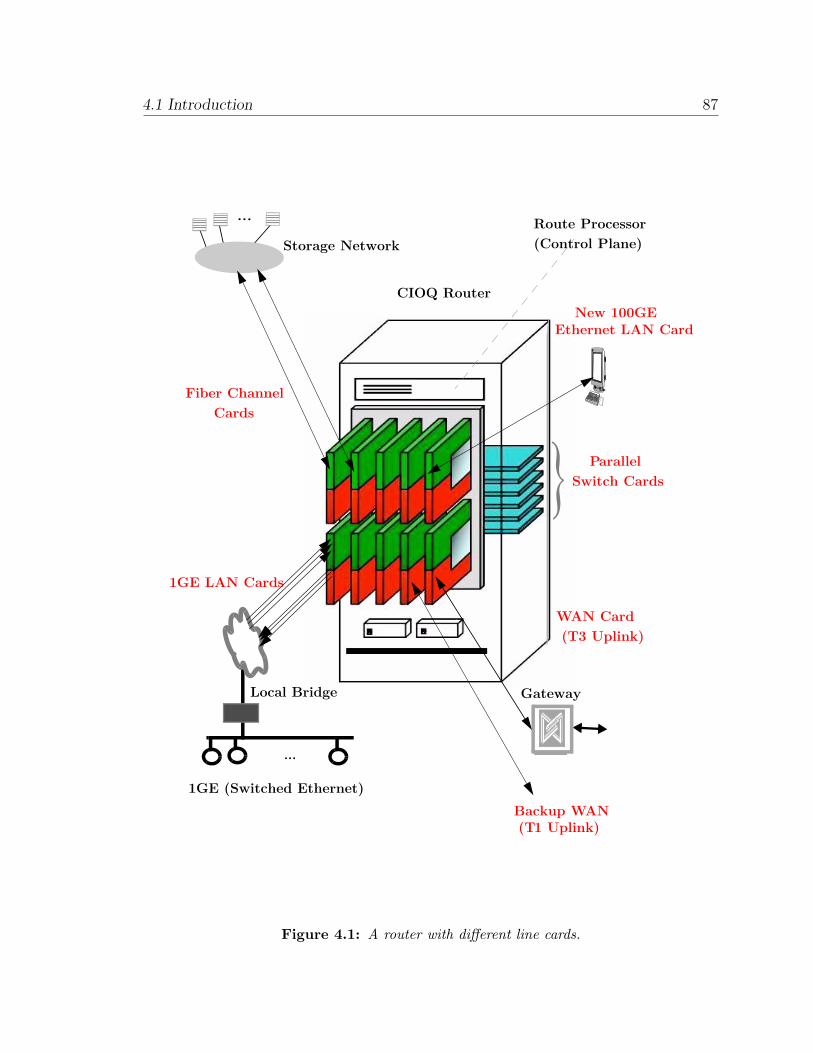
4.1 Introduction 87
1GE (Switched Ethernet)
Local Bridge
...
1GE LAN Cards
...
Storage Network
Fiber Channel Cards
WAN Card
Backup WAN(T1 Uplink)
(T3 Uplink)
Gateway
New 100GEEthernet LAN Card
Parallel Switch Cards
CIOQ Router
Route Processor(Control Plane)
Figure 4.1: A router with different line cards.

4.1 Introduction 88
4.1.1 A Note to the Reader
This chapter pertains to analytical work done over several years of research on CIOQ
routers by multiple researchers. Many CIOQ scheduling algorithms have been proposed
to obtain statistical guarantees (such as 100% throughput), as well as deterministic
performance guarantees such as work-conservation (to minimize average delay) and
emulation of an OQ router (to minimize the worst-case delay faced by packets). In
this chapter, we only focus on the emulation of an OQ router, and we consider both
FCFS and PIFO queuing policies. If a CIOQ router emulates an OQ router, then it
automatically guarantees 100% throughput and is also work-conserving.
We make several fine points in this chapter and attempt to succinctly capture the
underlying theory behind the emulation of OQ routers. We want to do three things
— (1) present the existing theory in a very simple manner, (2) derive more intuitive
algorithms that emulate an OQ router using the pigeonhole principle, and (3) re-state
previously known results in terms of the pigeonhole principle.
In order to do this, we present the material in an order which is not chronological,
but which builds up the theory step by step. We present only the results that, in
hindsight, are insightful and clarifying to the reader.2
4.1.2 Methodology
We will use our constraint set technique (first described in Chapter 2) which is a
formal way to apply the pigeonhole principle and analyze the CIOQ router. We will
consider the crossbar-based CIOQ router, since this is the most common switch fabric
deployed today. However, as we will see, this basic application of constraint sets has
two problems when it is applied to this non-single-buffered router — (1) It requires
us to make certain assumptions about the arrival traffic, and (2) It is only useful in
analyzing an FCFS CIOQ router; we cannot analyze a PIFO-CIOQ router.
As we will see, the main reason why we cannot analyze a PIFO-CIOQ router is
that the basic constraint set technique attempts to specify the transfer time of a packet
2A chronological order of the related work is described in Section 4.10.

4.2 Architecture of a Crossbar-based CIOQ Router 89
to the output line card as soon as the packet arrives. It does not take full advantage of
the architecture of a CIOQ router — i.e., the switch fabric does not immediately need
to commit to transferring packets that are waiting in the input line card, especially if
there are more urgent packets destined to the same output.
Therefore, in the later part of this chapter, we will extend the constraint set
technique to analyze and take advantage of the architecture of the (non-single-buffered)
CIOQ router. We will show that this extended constraint set technique allows us to
analyze both FCFS and PIFO CIOQ routers without making any assumptions about
the arrival traffic. As we will see, this requires us to use a class of algorithms called
stable matching algorithms [63] to schedule the crossbar, so as to meet the conditions
mandated by the extended constraint set technique.
4.2 Architecture of a Crossbar-based CIOQ
Router
Figure 4.2 shows an example of a crossbar-based CIOQ router. We denote the CIOQ
router to have a speedup of S, for S ∈ 1, 2, 3, . . . , N if it can remove up to S cells
from each input and transfer at most S cells to each output in a time slot. Note that
the CIOQ router can be considered to be a generalization of the IQ router and the
OQ router. At one extreme, in an IQ router (i.e., S = 1) only one cell can reach the
output from every input in a time slot. At the other extreme, in an OQ router (i.e.,
S = N), all the arriving N cells can be transferred to a specific output in a given time
slot.
The crossbar-based CIOQ router shown in the figure has a speedup of S = 2, and
has N = 8 ports. As described in Chapter 3, a crossbar fabric is restricted to perform
a matching (i.e., a permutation) between inputs and outputs in every time slot. If the
crossbar has a speedup S, then it can perform two independent matchings in every
time slot, as shown in Figure 4.2.
We will assume that cells are logically arranged on each line card as N virtual
output queues (VOQs). VOQs allow an input to group cells for each output separately,

4.3 Background 90
SNR
R
R
Line card #1
Line card #2 Line card #2
Line card #1
R
R
Line card #8 Line card #8
. .
3R
Switch Fabric
3R
3R3R
VOQs
R R
1 write, S reads S writes, 1 read
OQ
(Logical View) (Logical View)
..
1
2
8
1
2
8
Figure 4.2: The physical and logical view of a CIOQ router with crossbar speedup SNR =2NR.
and so a total of N2 VOQs are maintained in the router. VOQs are needed to prevent
head of line blocking [64]. Head of line blocking occurs when the head-of-line cell c,
queued at some input i, destined to some output j, prevents other cells at input i
from being scheduled. This can occur if output j is receiving cells from some other
input in the same time slot. Hence cell c cannot be scheduled (because its output j is
busy), while cells queued behind c (destined to other outputs) cannot be scheduled
because they are not at the head of the input queue.
4.3 Background
In [65], Charny proved that a CIOQ router can emulate an FCFS-OQ router under
restricted arrival traffic. Her algorithm was motivated by the following nice idea, i.e.,

4.3 Background 91
DIdea. “We can use maximal matchinga scheduling algorithms to emulate an
FCFS-OQ router”.
aIn a maximal matching, by definition, if there is a packet waiting at input i destinedto output j, then either input i or output j is part of the matching.
We will first present her proof, and then derive a simpler and more intuitive proof
based on the pigeonhole principle.
4.3.1 Charny’s Proof
Charny [65] placed the following restrictions on the arrival traffic when she analyzed
the CIOQ router:
1. Outputs can only be nitely congested: Charny constrained the arriving
traffic to be single leaky bucket constrained. The arriving traffic is said to be single
leaky bucket constrained if for every output j, the number of cells that arrive
destined to j in the time interval (t1, t2) is given by N(t1, t2) 6 λj(t2 − t1) +Bj ,
where Bj is some constant, and 0 6 λj < 1 for the traffic to be admissible.3
Note that if λj > 1, then output j receives more traffic than it can handle in
the long term – this means that we need a router that supports a faster line
rate! We can see that the above traffic constraint is equivalent to assuming that
the shadow OQ router has a finite buffer size Bj for every output, and that no
output is over-subscribed. If any output becomes congested and has more than
Bj cells destined to it temporarily, then such cells are dropped.
2. Inputs can only receive one cell per time slot: Charny restricted the
arrival traffic model such that no more than one cell can arrive at each input of
the CIOQ router, in any given time slot.
In practice, both the above restrictions are always true:
3Refer to Appendix B for an exact definition.

4.3 Background 92
1. Router buffers are finite and their size is determined during design. If we let
B = max∀j, Bj, then the output buffer size is bounded by B.
2. Cells arrive on physical links, and even though there may be multiple input
channels that can send cells in parallel, there is a cumulative maximum rate at
which a single cell can arrive.
We are now ready to present the main theorem in Charny’s work [65]:
Theorem 4.1. (Sufficiency, by Reference) Any maximal algorithm with a speedup
S > 2, which gives preference to cells that arrive earlier,4 ensures that any cell arriving
at time t will be delivered to its output at a time no greater than t+ [B/(S − 2)], if
the traffic is single leaky bucket B constrained.
Proof. This is proved in section 2.3, Theorem 5 of [65].5 We provide the outline of the
proof here. Charny uses a maximal matching algorithm (called oldest cell first) that
gives priority to cells that arrive earlier to the CIOQ router, and uses the fact that
for any maximal algorithm, if there is a cell waiting at input i destined to output j,
then either input i is matched or output j is matched (or both).6 The proof counts all
cells (called competing cells) that can prevent a particular cell from being transferred,
and classifies the competing cells into two types – cells at input i, or cells destined
to output j. It is shown that after a cell arrives, it cannot be prevented from being
transferred to output j for more than [B/(S − 2)] time slots. r
4.3.2 Why Is Charny’s Proof Complex?
The argument presented in Charny’s proof above is somewhat complex, for two reasons.
Consider any cell c:
1. Cell c can be repeatedly prevented – by competing cells arriving to the same
input later than it – from being transferred to its output over multiple time slots.
It would be nice if we can prevent this from happening.
4This is defined in section 2.3 in [65].5Charny uses a dual leaky bucket traffic model. The result in [65] has been restated here for the
single leaky bucket model to facilitate comparison between Theorem 4.2 and 4.1.6A similar analysis was used in [22].

4.4 Analyzing FCFS-OQ Routers Using the Pigeonhole Principle 93
2. Cell c can be overtaken – by competing cells arriving later at different inputs but
destined to the same output as cell c – and potentially prevented from getting
serviced by the output. It would be nice if we can somehow ensure that this does
not affect when cell c gets serviced by the output.
In what follows, we solve both the above problems [66] by fixing the time at which
a cell is transferred from the input to the output (“transfer time”), as soon as it arrives.
In this way, the time at which a cell is serviced by the output can’t be affected by
cells arriving later than it.
NObservation 4.1. Note that fixing a cell’s transfer time does not prevent the cell
from being overtaken by other cells arriving later at different inputs,
but destined to the same output. It merely ensures that these other
cells do not affect the time at which cell c gets serviced by the output.
4.4 Analyzing FCFS-OQ Routers Using the Pi-
geonhole Principle
First consider the physical structure of the crossbar CIOQ router. If a cell c arrives at
input i destined for output j, the router is constrained to transfer the cell only when
input i and output j are both free. So we can think of cells contending with cell c
(because they are from input i or destined to output j) as pigeons, contending for a
transfer time (pigeonholes). As described in Chapter 2, constraint sets are a convenient
accounting method to maintain and update this information. We are now ready to
analyze the conditions under which the CIOQ router will emulate an FCFS-OQ router.
We will use the algorithm described below, which is a direct consequence of the
pigeonhole principle. More formally, the algorithm is an example of a time reservation
algorithm [67, 68, 69, 70], since it reserves a future time for the arriving cell to be

4.4 Analyzing FCFS-OQ Routers Using the Pigeonhole Principle 94
transferred from the input to the output, immediately on arrival of a cell.
Algorithm 4.1: Constraint set-based time reservation algorithm.
input : Arrival and departure times of each cell.1
output : A transfer time for each cell.2
for each cell c do3
When a cell arrives at input i destined to output j with FCFS-OQ departure time4
DT , the cell is scheduled to depart at the first time in the future (larger than DT )
when both the input i and output j are free to participate in a matching.
We start by describing the algorithm when speedup S = 1, before generalizing to
larger speedup values:
1. Maintaining constraint sets: All inputs and outputs maintain a constraint
set. Each entry in the constraint set represents an opportunity to transmit a
cell in the future, one entry for each future time slot. For each future time slot
that an input is busy, the corresponding entry in its constraint set represents
a cell that it will transmit across the switch fabric to an output. Similarly, for
each future time slot that an output is busy, the entry represents a cell that it
will receive from one of the inputs. If, at some time in the future, there is no
cell to be transferred from an input (or to an output), then the corresponding
entry is free and may be used to schedule newly arriving cells.
2. Negotiating a constraint-free time to transfer: When a cell arrives at
input i destined to output j, input i communicates its input constraint set to
output j and requests a time in the future for it to transmit that cell. Output j
then picks the first time in the future tf in the interval (DT,DT +k) (where k is
a constant which we will determine shortly) for which both input i and output j
are free to transmit and receive a cell, i.e., time index tf is free in the constraint
sets of input i and output j. Output j grants input i the time slot tf in future
for transmitting the cell.

4.5 A Simple Proof to Emulate an FCFS CIOQ Router 95
DT -k - Bt
DTDT + k ......
c Spillover from previous k + B timeslots
Allocated departure time as seen by the input
Arriving cell c
DT - k
Figure 4.3: The constraint set as maintained by the input.
3. Updating constraint sets: Both input i and output j update their respec-
tive constraint sets to note the fact that time tf in the future is reserved for
transmitting the cell from input i to output j in the CIOQ router.
Note that, for any crossbar speedup S, an entry in the input constraint set is said
to be free in a particular time slot if the input is scheduled to send fewer than S
cells. Likewise, an entry in the output constraint set is said to be free if the output is
scheduled to receive fewer than S cells (from any input) in the corresponding time
slot.
4.5 A Simple Proof to Emulate an FCFS CIOQ
Router
We now use constraint sets to find the value of k for which every packet in the CIOQ
router is transferred from its input to its output within k time slots of its FCFS-OQ
departure time, i.e., tf 6 DT + k or tf ∈ (DT,DT + k) (where t is the arrival time of
a cell and k is a constant). The larger the speedup, the smaller the value of k.
Lemma 4.1. The number of time slots available in the input constraint set (ICS) for
any input i at any given time is greater than
[k − b(k +B)/Sc]. (4.1)

4.5 A Simple Proof to Emulate an FCFS CIOQ Router 96
Proof. Consider a cell that arrives to input i at time t, destined for output j with
FCFS-OQ departure time DT . The cell is scheduled to be transferred from input i to
output j in the CIOQ router in the interval (DT,DT + k), as shown in Figure 4.3.
Since the traffic is single leaky bucket (B) constrained, no cell that arrived before time
DT − B at input i has an FCFS-OQ departure time in the interval (DT,DT + k).
Hence, no cell that arrived before time DT − (B + k) at input i is allocated to be
transferred from input i in the CIOQ router in the interval (DT,DT + k). If the
speedup is S, then the number of time slots available in the input constraint set for
the newly arriving cell is at least [k − b(k +B)/Sc]. r
Example 4.2. Consider a CIOQ router with B = 100 and k = 150. Assume that
until now all cells have been given a transfer time within k = 150
time slots of its FCFS-OQ departure time, DT . Consider a cell c that
arrives at time t = 1000. If it came to the shadow OQ router, it can
never see more than B = 100 cells waiting at its output. Its FCFS-OQ
departure time, DT (which is allocated by the shadow OQ router
based on the number of cells already at the output) will be in the time
interval [1000, 1100]. Say, DT = 1055. We will attempt to give cell c
a transfer time within k = 150 time slots of DT , i.e., in the interval
[1055, 1205]. How many cells could have already requested a transfer
time between [1055, 1205] at the time of arrival? Definitely, no cells
that arrived before time 1055− 100− 150 = 805. For example, the
cell that arrived at time 804, must have had a departure time less than
904 and hence a transfer time lesser than 1054, and will not interfere
with our cell c. If not, it would violate the fact that until now all cells
have been given a transfer time which is within k = 150 time slots of
its FCFS-OQ departure time.

4.5 A Simple Proof to Emulate an FCFS CIOQ Router 97
DT - k
t
DTDT + k ......
c Spillover from previous k timeslots
Allocated departure time as seen by the output
Arriving cell c Figure 4.4: The constraint set as maintained by the output.
Lemma 4.2. The number of time slots available in the output constraint set (OCS)
for any output at any given time is greater than
[k − b(k/S)c]. (4.2)
Proof. Consider a cell that arrives at input i at time t, destined for output j with
FCFS-OQ departure time DT . The cell is scheduled to be transferred from input i to
output j in the CIOQ router in the interval (DT,DT + k), as shown in Figure 4.4.
Since all cells are scheduled to be transferred in the CIOQ router within k time
slots of their FCFS-OQ departure time, no more than k cells that have FCFS-OQ
departure times in the interval (DT − k,DT − 1) can already have been allocated to
be transferred to output j in the CIOQ router in the interval (DT,DT + k). Thus, if
the speedup is S, then the number of time slots available in the output constraint set
for the newly arriving cell is at least [k − b(k/S)c.7 r
Lemma 4.3. (Sufficiency) With a speedup S > 2, the algorithm ensures that each
cell in the CIOQ router is delivered to its output within [B/(S − 2)] time slots of its
FCFS-OQ departure time, if the traffic is single leaky bucket B constrained.
7We do not consider cells that have an FCFS-OQ departure time in the interval (DT + 1; DT + k),since the output policy is FCFS and these cells will be considered only after cell c is allocated a timetf ∈ (DT + 1; DT + k) for it to be transferred from input to output in the CIOQ router.

4.5 A Simple Proof to Emulate an FCFS CIOQ Router 98
Proof. (Using constraint sets). Consider a cell that arrives at time t. It should
be allocated a time slot tf for departure such that tf ∈ ICS ∩ OCS. A suffi-
cient condition to satisfy this is that [k − b(k +B)/Sc] > 0, [k − bk/Sc] > 0, and
[k − b(k +B)/Sc+ k − bk/Sc] > k. This is always true if we choose k > B/(S − 2).r
Theorem 4.2. (Sufficiency) With a speedup S > 2, a crossbar can emulate an FCFS-
OQ router if the traffic is single leaky bucket B constrained.
Proof. This follows from Lemma 4.3. r
By showing that the FCFS-CIOQ router emulates an FCFS-OQ router, it immediately
follows from Theorem 4.2 that the router has bounded delay, and 100% throughput.
4.5.1 Interesting Consequences of the Time Reservation Al-
gorithm
The time reservation algorithm, which is a consequence of using constraint sets, has
three interesting consequences:
1. The application of the constraint set technique leads to an intuitive understanding
of the scheduling constraints of the crossbar, and leads to a simpler scheduling
algorithm. It simplifies Charny’s well-known result (Theorem 4.1).
2. A more general result was later proved by Dai and Prabhakar (using fluid
models) [12], and later by Leonardi et al. [71] using Lyapunov functions. However,
unlike the work in [12] and [71], constraint sets lead to a hard bound on the
worst-case delay faced by a packet in the CIOQ router. In other words, when
subject to the same leaky bucket constrained arrival patterns, cells depart from
the CIOQ router and the FCFS-OQ router at the same time, or at least within
a fixed bound of each other.
3. The algorithm does not distinguish arriving cells based on their output desti-
nation. It only requires arriving cells to be stored in an input queue sorted
based on their allocated departure time, irrespective of the outputs that they

4.6 The Problem with Time Reservation Algorithms 99
are destined to. This means that line cards do not need VOQs, and it leads to
different queuing architectures.
4.6 The Problem with Time Reservation Algo-
rithms
There are two problems with the analysis described above — (1) We had to assume
that the buffers were finite, and (2) We have no simple way to extend the analysis to a
PIFO CIOQ router. While the former is a practical assumption to make,8 it is difficult
to see how we can extend the time reservation algorithm to support a PIFO queueing
policy. This is because we fixed the time at which a cell is transferred at the time
of its arrival. If later cells that were of higher priority came to the same input, they
would not be able to use the time slots that were allocated to the lower priority cells
(which may be destined to the same or even different outputs) that arrived earlier. If
we look at Figure 4.3 and Figure 4.4, the number of cells that compete for the same
interval (DT,DT + k) can be unbounded since cells arriving later can be of higher
priority, and this can happen indefinitely. This is a problem with any time reservation
algorithm.
In summary, the main problem with time reservation algorithms is that every
arriving cell c immediately contends for a time slot to be transferred to the output,
even though it may not be scheduled for departure until some time in the future. This
can happen because there are other cells already at the output that depart before cell
c, or that it have a much lower priority than other cells that are already destined to cell
c’s output. So we need some way to delay such a cell c from immediately contending
for a time slot. More generally, we need some way to indicate to the scheduler that
cell c has a lower priority for transfer, so that the scheduler may choose to schedule
some other higher-priority cell instead of cell c.
8In what follows, we will see that we can eliminate this assumption too.

4.7 A Preferred Marriage Algorithm for Emulating PIFO-OQ Routers 100
4.7 A Preferred Marriage Algorithm for Emulat-
ing PIFO-OQ Routers
Chuang et al [13] were the first to show that if the priority of cells could be conveyed
via a preference list by each input and output to a scheduler (without scheduling cells
immediately on arrival), then it is possible for a CIOQ router to emulate a PIFO-OQ
router. Their main idea was that a central scheduler would compute a matching
(marriage) between the inputs and outputs based on their preferences for each other.
The preferred marriages that are computed have the property that they are stable.
(See Box 4.1.)
They introduce a counting technique and monitor the progress of every cell9 to
ensure that it reaches its output on time, as compared to a PIFO-OQ router.
In what follows, our goal is to show that the counting technique introduced in [13]
can be viewed as a re-statement of the pigeonhole principle. We will see that in order
to do this, we will have to:
1. Indicate the priority of cells to the scheduler (Section 4.8.1),
2. Extend the application of the pigeonhole principle to make it aware of cell
priorities (Section 4.8.2), and,
3. Find the conditions under which this extended pigeonhole principle is satisfied
(Section 4.8.3).
9The authors do this via the use of a variable called slackness.

4.7 A Preferred Marriage Algorithm for Emulating PIFO-OQ Routers 101
Box 4.1: The Stable Marriage Problem
Consider the following succint description of stable marriages, defined in [72] —
Inputs Outputs
1
2
3
4
1
2
3
4
Woman 1 and Man 2 get their worst preferences
(3, 2, 4, 1)
(2, 3, 4, 1)
(2, 3, 4, 1)
(2, 4, 3, 1)
(3, 1, 4, 2)
(1, 3, 4, 2)
(1, 4, 3, 2)
(4, 1, 3, 2)
(Men) (Women)
but no one wants to switch
Figure 4.5: A stable marriage
Stable Marriages: Given N men and N
women, where each person has ranked all
members of the opposite sex with a unique
number between 1 and N in order of pref-
erence, marry the men and women off such
that there are no two people of opposite sex
who would both rather have each other than
their current partners. If there are no such
people, the marriages are “stable”.
An easier way to understand this is captured in the following quote [73] which
presupposes a married woman who professes interest in marrying another man. If she
receives the reply, “Madam, I am flattered by your attention, but I am married to someone
I love more than you, so I am not interested”, and this happens to any woman who wants
to switch (or vice versa) then the set of marriages is said to be stable.
NObservation 4.2. The algorithm was first applied for pairing medical students to hospital
jobs, and an example is shown in Figure 4.5. Gale and Shapely [63] proved
that there is always a set of stable marriages, irrespective of the preference
lists. The latter fact is key to analyzing crossbar routers.
In a CIOQ router, inputs and outputs maintain a priority list as described in Sec-
tion 4.8.1. The output prefers inputs based on the position of cells in its output priority
queue, i.e., based on the departure order of cells destined to that output. Similarly, inputs
prefer outputs based on the position of the cells in the input priority queues. In the context
of routers, a set of marriages is a matching. Since there is always a stable marriage, a
stable matching ensures that for every cell c waiting at an input queue:
1. Cell c is part of the matching.
2. A cell that is ahead of c in its input priority list is part of the matching.
3. A cell that is ahead of c in its output priority list is part of the matching.
So we can say that for every cell that is not transferred to its output in a scheduling
phase, the number of contentions will decrease by one in every matching. With speedup
two, this is enough to satisfy Property 4.1, which is required to emulate an OQ router.

4.8 A Re-statement of the Proof 102
2NR
A5B7B8C7 A6C9
A1Output Queue A
A4
B1Output Queue B
B3
C2C4C5C6
Output Queue C
C3
B4B5
C8
Cells ahead of C7 Cells ahead of C7
C7 : 4 Constraints (Pigeons) C7: 5 Opportunities (Pigeon Holes)
A7
B2A8
Input Priority Queue C
Input Priority Queue B
Input Priority Queue A
Figure 4.6: Indicating the priority of cells to the scheduler.
4.8 A Re-statement of the Proof
4.8.1 Indicating the Priority of Cells to the Scheduler
In order to convey the priority of cells to a scheduler, we will need a priority queue to
indicate the departure order of cells to the scheduler. A priority queue (as shown in
Figure 4.6), gives the scheduler flexibility in servicing higher-priority cells that are
still at their inputs, irrespective of their arrival time. The queue has the following
features:10
1. Arriving packets are “pushed-in” to an arbitrary location in the queue, based on
their departure order.
2. The position of the packets in the queue determines their priority of departure.
3. Once the packet is inserted, the relative ordering between packets in the queue
does not change.
4. A packet can depart from an arbitrary location in the queue if packets ahead of
it in the queue are unable to depart.
10Since a cell can leave from an arbitrary location in a priority queue, it has been referred to as apush in random out (PIRO) queue in literature [13].

4.8 A Re-statement of the Proof 103
Example 4.3. The example in the figure shows a 3x3 CIOQ router. The ports are
labelled A, B, and C. The input priority queue for ports A, B, C,
and the three output queues for ports A, B, and C are shown. In the
example shown, cells A5, A6, B7, B8, C7, and C9 are at the input
priority queue for port C. None of the cells in the input priority queue
are as yet scheduled. The input indicates to the scheduler the priority
of the cells via its input priority queue. For example, cell C7 has lower
priority than cells A5, A6, B7, and B8; however, it has higher priority
than cell C9. In a given time slot, if the scheduler matches output
ports A and B to some other inputs, then cell C7 can be scheduled to
leave before cells A5, A6, B7, and B8.
Why does cell C7 have a lower priority than, say, cell B8? We can see from the
figure that cell C7 has five cells — C2, C3, C4, C5, and C6 — that are ahead of it at
output port C. This means that cell C7 does not have to be scheduled in the next
five time slots. However, cell B8 has only four cells — B1, B3, B4 and B5 — ahead
of it in output port C. So, in a sense, cell B8 has to more urgently reach its output
than cell C7.
NObservation 4.3. Note that the introduction of a priority queue does not prevent
cells from being queued in VOQs. In fact, there are two choices for
implementation — (1) The cells may be queued in VOQs, or segregated
further into queues based on differentiated classes of service for an
output. An input priority queue is maintained separately to describe
the order of priority between these cells, or (2) We can do away with
VOQs altogether; the cells can be queued directly in an input priority
queue.
4.8.2 Extending the Pigeonhole Principle
We can state the observations from Example 4.3 in terms of pigeons and pigeonholes.

4.8 A Re-statement of the Proof 104
1. Pigeons: For every cell c, the cells that are ahead of it in the input priority
queue contend with it for a time slot, so that they can be transferred to their
respective outputs. These cells are similar to contending pigeons.
2. Pigeonholes: Every cell that is already at cell c’s output and has an earlier
departure time than cell c allows the cell more time to reach its output. These
cells represent distinct opportunities in time for cell c to be transferred to the
output. We will use pigeonholes to represent these opportunities.
In order to ensure that cells waiting in the input priority queue reach the output
on time, we will mandate the following inequality: the number of opportunities
(pigeonholes) for a cell is always equal to or greater than the number of cells that
contend with it (pigeons). This inequality must be satisfied for every cell, as long as it
resides in the input priority queue.
Let us contrast this to our analysis of SB routers. In an SB router, a cell gets
allocated to a memory on arrival. This memory is available to the output when the
cell needs to be read at its departure time. So, we can forget about the cell once it
has been allocated to a memory. In contrast, in a CIOQ router, the cell may remain
in the input priority queue for some time before it is transferred to the output. So we
have to continually monitor the cell to ensure that it can reach the output on time for
it to depart from the router. This is formalized in Algorithm 4.2.
We maintain two constraint sets to track the evolution of every cell — (1) An
opportunity set (pigeonholes) that constrains the number of time slots that are available
for a cell to be transferred, and (2) A contention set (pigeons) to track the cells that
contend with a cell and prevent it from being transferred to its output.
Example 4.4. Table 4.1 shows an example of the opportunity and contention sets for
each cell in the input priority queue for port C of Figure 4.6. Both these
sets are easily derived from the position of the cell in its input priority
queue and the state of the output queue as shown in Figure 4.6. Note
that for every cell in Table 4.1, the number of opportunities (column
5) is currently greater than the number of contentions (column 3).

4.8 A Re-statement of the Proof 105
Algorithm 4.2: Extended constraint sets for emulation of OQ routers.
input : CIOQ Router Architecture.1
output: A bound on the number of memories, total memory, and switching2
bandwidth required to emulate an OQ router.
for each cell c which arrives at time T and departs at time DT do3
for t←∈ T, T + 1, . . . , DT do4
Opportunity Set (pigeonholes) ← cells ahead of c, already at its output5
Contention Set (pigeons) ← cells ahead of c at its input6
if cell c is still at the input then7
Ensure: |Pigeonholes| ≥ |Pigeons|.8
Table 4.1: An example of the extended pigeonhole principle.
Cell Cells Ahead in Input #Contentions Cells Ahead in Output #Opportunities(Pigeonholes) (Pigeons)
A5 - 0 A1,A4 2
A6 A5 1 A1,A4 2B7 A5,A6 2 B1,B3,B4,B5 4B8 A5,A6,B7 3 B1,B3,B4,B5 4
C7 A5,A6,B7,B8 4 C2,C3,C4,C5,C6 5C9 A5,A6,B7,B8,C8 5 C2,C3,C4,C5,C6,C8 6
4.8.3 Using Induction to Enforce the Pigeonhole Principle
How do we ensure that the conditions described in Algorithm 4.2 are met? To do this,
we use simple induction to track the change in size of the contention and opportunity
set in every time slot that a cell waits at the input. But we have two problems — (1)
In every time slot, for every cell, it is possible that the contention set increases in size
by one, due to newly arriving cells that may have higher priority than it. Also, the
opportunity set will decrease in size by one, because a cell will depart from the output.
The former increases the number of pigeons, while the latter decreases the number of
pigeonholes available for the cell. Both of these are detrimental from the cell’s point
of view, and (2) When a cell arrives, it is inserted into the input priority queue. At
the time of insertion, it must at least have equal or more opportunities as the number
of contenting cells. If not, it may never make it to the output on time.

4.9 Emulating FCFS and PIFO-OQ Routers 106
So, in order to meet the induction step (between consecutive time slots that the
cell waits at the input) and the induction basis case (at the time slot when a cell
arrives to the input), we mandate the following properties:
DProperty 4.1. Induction Step: In every time slot, the switch scheduler does the
following at least twice — it either decrements the size of the contention
set or increments the size of the opportunity set for every cell waiting at
the input, i.e., it either decrements the number of pigeons or increments
the number of pigeonholes for every cell.
DProperty 4.2. Induction Basis Case: On arrival, a cell is inserted into a position
in the input priority queue such that it has equal or more opportunities
to leave than the number of contentions, i.e., it has equal or more
pigeonholes than the number of pigeons.
4.9 Emulating FCFS and PIFO-OQ Routers Using
the Extended Pigeonhole Principle
We have shown that the method of proof introduced in [13] is simply a re-statement of
the pigeonhole principle, applied to every cell for every time slot that it waits at the
input. We are now ready to re-state the results for the preferred marriage algorithm
in [13] as follows — If Property 4.1 and Property 4.2 are met, the conditions for the
extended constraint set technique (Algorithm 4.2) are satisfied. It follows that all cells
reach their output on time, and a CIOQ router can emulate a PIFO-OQ router.
In order to satisfy Property 4.1, the authors [13] ensure that the preferred marriages
are stable [63], and operate the crossbar at speedup S = 2. Also, in order to satisfy
Property 4.2, the authors insert an arriving cell as far ahead in the input priority
queue as required so that it has more opportunities than the number of contending
cells at the time of insertion.11 In an extreme case, the arriving cell may have to be
11Note that there are many insertion policies that satisfy Property 4.2, since we only need to insertan arriving cell at any position where it has more opportunities than the number of contending cells.

4.10 Related Work 107
inserted at the head of line. Note that the memories in the input line cards need
to run at rate 3R (to support one write for the arriving cell, and up to two reads
into the crossbar). The memories in the output line cards also need to run at 3R (to
support two writes for cells arriving from the crossbar, and one read to send a cell to
the output line). This requires a total memory bandwidth of 6NR. We can now state
the following theorem:
Theorem 4.3. (Sufficiency, by Citation) A crossbar CIOQ router can emulate a
PIFO-OQ router with a crossbar bandwidth of 2NR and a total memory bandwidth of
6NR.
Proof. Refer to [13] for the original proof. r
4.10 Related Work
In what follows, we present a brief chronological history of the research in CIOQ
routers. Due to the large body of previous work, this section is by no means exhaustive,
and we only present some of the key salient results.
4.10.1 Statistical Guarantees
We first consider CIOQ routers with crossbar speedup S = 1. Recall that such a CIOQ
router is simply an IQ router. IQ routers that maintain a single FIFO buffer at their
inputs are known to suffer from head-of-line blocking. Karol et al. [64] showed that the
throughput of the IQ router is limited to 58% when the input traffic is independent,
identically distributed (i.i.d)12 Bernoulli, and the output destinations are uniform.
Based on the negative results in [64], several authors [75, 76, 77, 78] did analytical
and simulation studies of a CIOQ router (which maintains a single FIFO at each
input) for various values of speedup. These studies show that with a speedup of four
to five, one can achieve about 99% throughput when arrivals are i.i.d at each input
and when the distribution of packet destinations is uniform across the outputs.
12Refer to Appendix B for an exact definition.

4.10 Related Work 108
Box 4.2: The Stability of Forced Marriages
The algorithm described to emulate an OQ router in Section 4.9 is an example ofpreferred marriage. Inputs and outputs maintain preference lists and communicate theirchoices to a central scheduler. The central scheduler computes a stable marriage andattempts to satisfy (to the best of its abilities) the preferences of the inputs and the outputs.
Suppose we deny the inputs and outputs choice. We can ask — What happens ifthe matchings (marriages) that we compute are forced marriages?a Prabhakar et al [41]describe an algorithm called MUCFA (Most Urgent Cell First Algorithm) whose analogyto forced marriages is as follows:
MUCFA:When a cell arrives it is given an urgency, which is the time remainingfor it to leave the OQ router. A cell progressively becomes more urgent in every timeslot. In each scheduling phase, an input is forced to prefer outputs that have more urgentcells, and outputs are forced to prefer inputs based on which inputs have more urgent cells.The preferences lists are created simply as a consequence of the urgency of a cell. Inputsand outputs have no say in the matter. In each scheduling phase, a centralized schedulercomputes a forced marriage which is stable.
The stable forced marriage computed by MUCFA gives priority to more urgent cellsand has the following property. For every cell c waiting at an input queue:
1. Cell c is part of the matching.2. A cell that is more urgent than c in its input priority list is part of the matching.3. A cell that is more urgent than c in its output priority list is part of the matching.
Prabhakar et al. [41] show using a reductio-ad-absurdum argument that MUCFA canemulate an OQ router with speedup four.
NObservation 4.4. It is interesting to apply the pigeonhole principle to analyze MUCFA. Itcan be easily seen that MUCFA satisfies Property 4.1 with speedup two. Butthere is no easy way to know whether MUCFA satisfies the induction basecase, i.e., Property 4.2 on cell arrival. This is because unlike the preferredmarriage algorithm, MUCFA does not give choice to an input to insert anarriving cell into its preference list.
Coincidentally, similar to marriages in certain traditional societies, the algorithms forforced marriages for CIOQ routers [41] preceded the algorithms for preferred marriages [13].Note that both sets of marriages can be made stable, and are successful in emulating anOQ router.
It has been shown via counterexample [74] that MUCFA with speedup two cannotemulate an OQ router. However, it is not known whether MUCFA can emulate an OQrouter with speedup three, and this remains an interesting open problem.
aNot to be confused with arranged marriage, a much-maligned and misused term, incorrectlyused in the modern world to describe a large class of marriages!

4.10 Related Work 109
It was later shown that the low throughput of IQ routers is due to head-of-line
blocking, and it can be overcome using virtual output queues (VOQs) [79]. This led to a
renewed interest in IQ routers. Tassiulas and Ephremides [39] and McKeown et al. [11]
proved that an IQ router with VoQs can achieve 100% throughput with a maximum
weight matching (MWM) algorithm, if the input traffic is i.i.d and admissible; the
outputs are allowed to be non-uniformly loaded. Dai and Prabhakar [12] generalized
this result and showed that MWM can achieve 100% throughput provided that the
input traffic satisfies the strong law of large numbers and is admissible. However,
MWM is extremely complex to implement and has a time complexity, O(N3 logN).
A different approach was considered by Chang et al. [80] and Altman et al. [81].
They showed (using the results of Birkhoff [82] and von Neumann [83]) that the
crossbar can be scheduled by a fixed sequence of matchings (called frames)13 such
that the IQ router can achieve 100% throughput for any admissible arrival pattern.
These are similar to time division multiplexing (TDM) techniques in the switching
literature [84]. However, their usage of frame scheduling requires prior knowledge of
the arrival traffic pattern, and the router needs to maintain a potentially long sequence
of matchings, and so these techniques have not found usage in practice.
One would expect that the maximum size matching (MSM) algorithm, which
maximizes the instantaneous bandwidth of the crossbar (the most efficient algorithm
has a lower time complexity O(N2.5) [85, 86]), would also be able to achieve 100%
throughput. However, contrary to intuition, MSM is known to be unfair (if ties are
broken randomly), can lead to starvation, and hence cannot achieve 100% through-
put [87]. Not all MSM algorithms suffer from loss of throughput. In [88] it is shown
that the longest port first (LPF) algorithm (an MSM algorithm that uses weights to
break ties) achieves 100% throughput for Bernoulli arrivals.
In [89], Weller and Hajek give a detailed analysis on the stability of online matching
algorithms (including MSM) using frame scheduling with a constrained traffic model.
Our work in [90] extends some of the results in [89] by alleviating the traffic constraints
and considering stochastic (Bernoulli) arrivals. It shows that with a slight modification
13This is similar to the idea of frame scheduling described in Chapter 3.

4.10 Related Work 110
of frame scheduling (called batch scheduling), a class of MSM algorithms (called Critical
Maximum Size Matching, or CMSM), can achieve 100% throughput for (uniform or
non-uniform) Bernoulli i.i.d. traffic. Also, under the purview of batch scheduling,
the unfairness of MSM reported in [88] is eliminated, and any MSM algorithm can
achieve 100% throughput under Bernoulli i.i.d. uniform load. However, since the
batch scheduling MSM algorithms described above can suffer from large worst case
delay and have large time complexity, they are not used in practice.
There are two approaches that are more practical toward achieving 100% through-
put. They involve speeding up the crossbar or randomizing the MWM scheduler. Dai
and Prabhakar [12] in their seminal paper analyzed maximal matching algorithms
and proved that any maximal matching algorithm can achieve 100% throughput with
speedup, S = 2 for a wide class of input traffic. Subsequently, Leonardi et al. [71]
also proved a similar result. The authors in [36, 91, 92, 93] took a different approach.
They describe load balancing algorithms14 that are simple to implement and achieve
100% throughput. They come at the expense of requiring two switching stages, and
also require a higher crossbar speedup, S = 2.15
Tassiulas [94] showed that a randomized version of MWM (which is easier to
implement) can achieve 100% throughput with speedup, S = 1. Later, Giaccone et
al. [95] described other randomized algorithms that achieve 100% throughput with
S = 1 and also closely realize the delay performance of the MWM scheduler.
4.10.2 Deterministic Guarantees
The algorithms described above make no guarantees about the delay of individual
packets, and only consider average delay. The approach of mimicking (or emulating)
an OQ router was first formulated in [41]. They showed that a CIOQ router with a
speedup of four, and an algorithm called MUCFA (most urgent cell first algorithm),
14Note that the algorithms we proposed in [36] were first described for a parallel packet switcharchitecture, which is described in Section 6.7. But the results are immediately applicable to theCIOQ router.
15Note that when these algorithms have knowledge of the destination port of the incoming cell,they can emulate an FCFS-OQ router even under adversarial inputs.

4.10 Related Work 111
Box 4.3: Work Conservation without Emulation
A work-conserving router gives a deterministic performance guarantee— it alwayskeeps its outputs busy. In Chapter 1, we mandated FCFS-OQ emulation as a condition toachieve work-conservation. This gave us an additional deterministic performance guaranteefor each individual packet, i.e., it would leave at the same time as compared to an idealFCFS-OQ router. We can relax this condition. In what follows, we will show that we canalso apply the pigeonhole principle to find the conditions under which a CIOQ router iswork-conserving without mandating FCFS-OQ emulation.
For a router to be work-conserving, we only need to ensure that its outputs arekept busy. So, in such a router, the order of departures of packets from outputs isirrelevant. It is sufficient that some packet leave the output at all times that thecorresponding output in the shadow OQ router is also busy. So, from a cell’s perspective,it is sufficient that either (1) some cell ahead of it in the input priority list leave theinput, or (2) some cell (irrespective of its departure time) make it to the output inevery scheduling opportunity. So we can make the following simple modification to theextended constraint set technique in order that our CIOQ router be work-conserving:
Algorithm 4.3: Extended constraint sets for work conservation.
input : CIOQ Router Architecture.1
output : A bound on the number of memories, total memory and switching2
bandwidth required to emulate an OQ router.
for each cell c which arrives at time T and departs at time DT do3
for t←∈ T; T + 1; : : : ; DT do4
Opportunity Set (pigeonholes) ← any cells already at its output5
Contention Set (pigeons) ← cells ahead of c at its input6
if cell c is still at the input then7
Ensure: |Pigeonholes| ≥ |Pigeons|.8
As a consequence, the scheduler which ensures that the preferred marriages describedin Section 4.9 are stable (and which was used to ensure that a CIOQ router can emulate aPIFO router) can be simplified. It no longer needs to be aware of the priority between cellsdestined to the same output. This leads to the following theorem:
Theorem 4.4. A crossbar CIOQ router is work-conserving with a crossbar bandwidth of2NR and a total memory bandwidth of 6NR.
4.11 Conclusions 112
can emulate an OQ router for arbitrary input traffic patterns and router sizes. Later,
in their seminal paper [13], the authors improved upon the result in [41] and were the
first to show that a CIOQ router can emulate an OQ router with speedup two.
In contrast, Charny [65] also considered emulation, but required assumptions on the
arrival traffic and only considered FIFO traffic, while Krishna et al. [23] independently
showed that a CIOQ router is work-conserving with speedup two. Note that Stoica
et al. [96] also considered the emulation of a CIOQ router with speedup two. Their
paper had an error, which was later fixed [97] in consultation with the authors in [13].
Recently, Firoozshahian et al. [98] presented a surprising algorithm that (unlike all
other previous algorithms) only uses local information to emulate a constrained OQ
router that performs “port-ordered” scheduling policies.
4.11 Conclusions
We have extended the work done on providing delay guarantees in [65] and PIFO
emulation in [13], as follows:
1. Our work on time reservation algorithms, presented in Section 4.4 for the classical
unbuffered crossbar, extends Charny’s result [65]. In [65] it was shown that
a maximal matching algorithm would lead to the main result (Theorem 4.1).
The result relied on a scheduler that examines the contents of the input queues
during each time slot to determine which cells to schedule. In contrast, the
constraint set technique leads to an almost identical result (Theorem 4.2), using
a simpler algorithm that schedules cells as soon as they arrive. While algorithms
for IQ and CIOQ routers that schedule cells immediately upon arrival have been
proposed before [67, 68, 69, 70], we are not aware of any previous work that
shows when such algorithms can achieve 100% throughput, give bounded delay,
and emulate an FCFS-OQ router.
2. The analysis of non-SB routers was a hard problem, because cells that arrive
to non-SB routers do not get queued for their outputs immediately. They may
be held at one or more intermediate points before they are transferred to their

4.11 Conclusions 113
respective outputs. We introduced the extended constraint set technique, which
follows the path of the cell and enforces constraints on the cell on every time slot
before it reaches its output. The extended constraint set technique has given us
a powerful tool to analyze non-SB routers. It has clarified our understanding of
the results in [13] and brought it under the purview of the pigeonhole principle.
Summary
1. In this chapter, we analyze the combined input output queued (CIOQ) router. In a CIOQ
router, a packet is buffered twice — once when it arrives, and once before it leaves. The
first buffer is on the line card it arrives on. The second buffer is on the line card it departs
from.
2. Intuitively, the two buffers make the job easier for a central scheduler — if the switch is
not ready to transfer packets as soon as they arrive, it can hold them in the input line
card. Similarly, if the scheduler has the opportunity to send a packet to the output, it
doesn’t need to wait until the output line is free — the output line card will buffer it in
the output until the line is free.
3. We use the constraint set technique (introduced in Chapter 2) to analyze the conditions
under which a CIOQ router can emulate an OQ router.
4. The use of the constraint set technique implies that our scheduling algorithm attempts
to reserve a time slot (either now or in the future) to transfer a cell to the output line
card as soon as it arrives. As a consequence, our switching algorithm belongs to a class of
algorithms called “time reservation algorithms”.
5. We show that a CIOQ router (using a time reservation algorithm) with a crossbar band-
width greater than 2NR and a memory bandwidth greater than 6NR is work-conserving
(Theorem 4.4) and can emulate an FCFS-OQ router (Theorem 4.2).
6. Our techniques lead to an intuitive understanding of the constraints faced in a CIOQ
router, and also simplify the algorithms presented in [65].
7. However, we have to make assumptions (e.g., that the CIOQ router has a finite size buffer)
in order to prove the above results. While these assumptions are practical, the constraint
set technique unfortunately does not allow us to find the conditions under which a CIOQ
router can emulate an OQ router that provides qualities of service.

4.11 Conclusions 114
8. This is because the basic constraint set technique does not take full advantage of the
architecture of a CIOQ router as it commits to transferring a packet immediately on arrival.
9. We therefore introduce the extended constraint set technique to analyze the CIOQ router.
The extended constraint set technique is a re-statement of the counting principle introduced
in [13], and is a method to continuously track the progress of a cell while it waits at the
input, in its attempt to be transferred to the output.
10. We re-state the previously known results in [13] in terms of the extended constraint set
technique to show that a CIOQ router with a crossbar bandwidth of 2NR and a memory
bandwidth of 6NR can emulate an OQ router that supports multiple qualities of service
(Theorem 4.3).
11. The extended constraint set technique has broadened our understanding of routers. It
brings under the purview of the pigeonhole principle other router architectures that are
not single-buffered.

Chapter 5: Analyzing Buered CIOQ Routers
with Localized MemoriesFeb 2008, Santa Cruz, CA
Contents
5.1 Introduction . . . . . . . . . . . . . . . . . . . . . . . . . . . . . . . . 117
5.1.1 Goal . . . . . . . . . . . . . . . . . . . . . . . . . . . . . . . . . . . . . 118
5.1.2 Intuition . . . . . . . . . . . . . . . . . . . . . . . . . . . . . . . . . . . 118
5.2 Architecture of the Buffered CIOQ Router . . . . . . . . . . . . . . 120
5.2.1 Why Are Buffered Crossbars Practical? . . . . . . . . . . . . . . . . . 121
5.3 Applying the Pigeonhole Principle to Analyze Buffered Crossbars 123
5.3.1 Satisfying the Properties for the Extended Pigeonhole Principle . . . . 123
5.4 Analyzing Buffered FCFS-CIOQ Routers . . . . . . . . . . . . . . . 125
5.5 Crosspoint Blocking . . . . . . . . . . . . . . . . . . . . . . . . . . . . 126
5.6 Analyzing Buffered PIFO CIOQ Routers . . . . . . . . . . . . . . . 128
5.6.1 Emulating a PIFO-OQ Router by Recalling Cells . . . . . . . . . . . . 128
5.6.2 Emulating a PIFO-OQ Router by Bypassing Cells . . . . . . . . . . . 128
5.6.3 Emulating a PIFO-OQ Router by Disallowing Less Urgent Cells . . . 129
5.7 Conclusions . . . . . . . . . . . . . . . . . . . . . . . . . . . . . . . . . 133
List of Dependencies
• Background: The memory access time problem for routers is described in
Chapter 1. Section 1.5.2 describes the use of load balancing techniques, and
Section 1.5.3 describes the use of caching techniques; both these techniques are
used to alleviate the memory access time problems for the buffered CIOQ router.
Additional Readings
• Related Chapters: The load balancing technique to analyze the buffered
combined input output queued (CIOQ) router, introduced in this chapter, is
described in Section 4.9. The load balancing technique is also used to analyze
the CIOQ router architecture in Chapter 4.

Table: List of Symbols.
Bij Crosspoint for Input i, Output j
c, C CellDT Departure TimeN Number of Ports of a RouterR Line RateS Speedup
SV OQ Super VOQT Time Slot
Table: List of Abbreviations.
ASIC Application Specific Integrated CircuitCIOQ Combined Input Output Queued Router
eDRAM Embedded Dynamic Random Access MemoryFCFS First Come First Serve (Same as FIFO)OQ Output Queued
PIFO Push In First OutSB Single-buffered
QoS Quality of ServiceVOQ Virtual Output QueueWFQ Weighted Fair Queueing
“A (stable) marriage can be
ruined by a good memory”.
— Anonymous† 5Analyzing Buffered CIOQ Routers with
Localized Memories
5.1 Introduction
In Chapter 4, we introduced the combined input output queued (CIOQ) router. CIOQ
routers are widely used, partly because they have localized buffers that enable these
routers to be easily upgraded. However they are hard to scale because the scheduler
in a crossbar-based CIOQ router implements complex stable marriage algorithms [63].
This chapter is motivated by the following question: Can we simplify the scheduler to
make CIOQ routers more scalable? The main idea is as follows —
DIdea. “By introducing a small amount of buffering (similar to a cache) in the
crossbar, we can make the scheduler’s job much simpler. The intuition is that
when a packet is switched, it can wait in the buffer; it doesn’t have to wait until
both the input and output are free at the same time”.
In other words, our scheduler doesn’t have to resolve two constraints at the same
time. As we will see, this will reduce the complexity of the scheduler from O(N2) to
†The exact version of the quote differs in literature.
117

5.1 Introduction 118
O(N) and remove the need for a centralized scheduler. In this chapter, we’ll prove
that anything we can do with a CIOQ router, we can do simpler with a buffered CIOQ
router.
Example 5.1. Figure 5.1 shows a cross-sectional view of the crossbar ASIC in a
CIOQ router. As can be seen, the central crossbar has to interface with
all the line cards in the router. The current technology constraints are
such that the size of the crossbar ASIC is determined by the number of
interconnect pins. This leaves a large amount of on-chip area unused
in the crossbar ASIC, which can be used to store on-chip buffers.
5.1.1 Goal
Our goal is to make high-speed CIOQ routers practical to build, while still providing
deterministic performance guarantees. So, in what follows, we will not use complex
stable marriage algorithms [63]. Instead we consider a crossbar with buffers (henceforth
referred to as a “buffered crossbar”) and answer the question —What are the conditions
under which a buffered crossbar can emulate an OQ router that supports qualities of
service?
In what follows, we’ll show simple schedulers that make a buffered crossbar give
deterministic performance guarantees – and we’ll derive the conditions under which
they are work-conserving and can emulate an OQ router that supports qualities of
service.
5.1.2 Intuition
Researchers first noticed via simulation that the introduction of buffers to a crossbar
can provide good statistical guarantees. They showed that the buffered crossbar can
achieve high throughput for admissible uniform traffic with simple algorithms [99, 100,
101, 102]. Simulations also indicated that with a modest speedup, a buffered crossbar
can closely approximate fair queueing [103, 104]. This confirms our intuition that the
addition of a buffer can greatly enhance the performance of a crossbar-based fabric.

5.1 Introduction 119
Crossbar
Crossbar ASIC
Empty area on dieavailable for memory
Pin Limited
Switch Fabric(s)
Cross-sectional View of
Crossbar ASIC
Line
Front View of Crossbar-based CIOQ Router
Cards
LCLC
LC
LCLC
LC
Crossbar-based CIOQ Router
... .
Figure 5.1: Cross-sectional view of crossbar fabric.

5.2 Architecture of the Buffered CIOQ Router 120
R
R
R
Line card #1
Line card #2
Line card #1
R
Line card #3
2NR
Crossbar with
VOQs Crosspoint Buffering
1 cell per input-output pair
Line card #2
RVOQs
Line card #3
RVOQs
Figure 5.2: The architecture of a buffered crossbar with crosspoint buffer.
However, until recently there were no analytical results on guaranteed throughput
to explain or confirm the observations made by simulations. The first analytical results
were by Javidi et al. who proved that, with uniform traffic, a buffered crossbar can
achieve 100% throughput [105]. More recently, Magill et al. proved that a buffered
crossbar with a speedup of two can emulate an FCFS-OQ router [42, 106]. Magill et
al. also showed that a buffered crossbar with k cells per crosspoint can emulate an
FCFS-OQ router with k strict priorities.
5.2 Architecture of the Buered CIOQ Router
Figure 5.2 shows a 3× 3 buffered crossbar with line rate R. Similar to the crossbar
router, arriving packets are buffered locally on the same line card on which they arrive,
and held there temporarily. Later they are switched to the corresponding output
line card, where they are again held temporarily before they finally leave the router.
Fixed-length packets or cells wait in the VOQs to be transferred across the switch.
Each crosspoint contains a buffer that can cache one cell. The buffer between input i

5.2 Architecture of the Buffered CIOQ Router 121
and output j is denoted as Bij. When the buffer caches a cell, Bij = 1, else Bij = 0.
In a sense, when the buffer is non-empty, it contains the head of a VOQ, and thus
allows the output to peek into the state of the VOQ. Similar to the crossbar-based
CIOQ router in the previous chapter, the inputs maintain an input priority queue
(refer to Figure 4.6) to maintain the priority of cells. As in the previous chapter, there
are two choices for implementation — (1) Keep arriving cells in VOQs, and a separate
input priority queue to describe the order between the cells, or (2) Keep the cells
sorted directly in an input priority queue.
The key to creating a scheduling algorithm is determining the input and output
scheduling policy that decides how input and output schedulers pick cells. We will see
that different policies lead to different scheduling algorithms.
5.2.1 Why Are Buered Crossbars Practical?
Unlike a traditional crossbar, the addition of memory (which behaves like a cache)
in a buffered crossbar, obviates the need for the computation of complex stable
matching algorithms. This is because the inputs and outputs are no longer restricted
to performing a matching in every time slot, and have more more flexibility as described
below.
The scheduler for a buffered crossbar consists of 2N parts: N input schedulers
and N output schedulers. The input schedulers (independently and in parallel) pick a
cell from their inputs to be placed into an empty crosspoint. The output schedulers
(independently and in parallel) pick a cell from a non-empty crosspoint destined for
that output.
NObservation 5.1. A traditional crossbar fabric is limited to performing no more than
N ! permutations to match inputs to outputs. In contrast (depending
on the occupancy of the crosspoints), the buffered crossbar can allow
up to NN matchings between inputs and outputs.
The N input and N output schedulers can be distributed to run on each input
and output independently, eliminating the single centralized scheduler. They can be

5.2 Architecture of the Buffered CIOQ Router 122
pipelined to run at high speeds, making buffered crossbars appealing for high-speed
routers.
NObservation 5.2. It is interesting to compare this scheduler with the scheduler for
an unbuffered crossbar-based CIOQ router described in Chapter 4. The
scheduler in Chapter 4 also gave deterministic performance guarantees,
but in order to provide these guarantees, our scheduling algorithm
required the inputs and outputs to keep a list of preferences and convey
these preferences to a scheduler. This meant that the scheduler had
to be aware of the states of all inputs and outputs, and be centrally
located. The scheduler computed a matching by running a version of
the stable marriage algorithm [63]. In [13], the authors describe two
scheduling algorithms that can compute stable matching, the faster
of which still takes O(N) iterations to compute a matching. The
high communication overhead between the inputs and outputs, the
amount of state that needs to be maintained and communicated to the
centralized scheduler, and the implementation complexity, make stable
matching algorithms hard to scale when designing high-speed routers.
Of course, simplifying the scheduler requires a more complicated crossbar capable
of holding and maintaining N2 packet buffers on-chip. In the past, this would have
been prohibitively complex: the number of ports and the capacity of a crossbar switch
were formerly limited by the N2 crosspoints that dominated the chip area; hence the
development of multi-stage switch fabrics, e.g., the Clos, Banyan, and Omega switches,
based on smaller crossbar elements. Now, however, crossbar switches are limited by
the number of pins required to get data on and off the chip [107].
Example 5.2. Improvements in process technology, and reductions in geometries,
mean that the logic required for N2 crosspoints is small compared to
the chip size required for N inputs and N outputs. The chips are
pad-limited, with an under-utilized die. A buffered crossbar can use the

5.3 Applying the Pigeonhole Principle to Analyze Buffered Crossbars 123
unused die for buffers, and further improvements in on-chip eDRAM
memory technology [26] allow for storing a large amount of memory
on-chip. With upcoming 45nm chip technology, ∼128Mb of eDRAM
can easily fit on an average chip. This can easily support a 256× 256
router (with 256-byte cells), making a buffered crossbar a practical
proposition.1
5.3 Applying the Pigeonhole Principle to Analyze
Buered Crossbars
In Chapter 4, we introduced the extended pigeonhole principle (Algorithm 4.2) as a
general technique to analyze whether a router can emulate an OQ router (and as a
consequence give deterministic performance guarantees). The crossbar-based CIOQ
router in Chapter 4 was able to emulate an OQ router because the stable matching
algorithms that we described (and first mentioned in [13]) ensured that the pigeonhole
principle is satisfied for every cell in every time slot.
5.3.1 Satisfying the Properties for the Extended Pigeonhole
Principle
Since we are also interested in emulating an OQ router, we will choose a scheduling
algorithm that also attempts to satisfy the conditions of the pigeonhole principle.
Our scheduling algorithm consists of two parts, one each for the input and the
output scheduler. This is shown in Algorithm 5.1. To show that our scheduling
algorithm meets the pigeonhole principle, recall the two properties that we introduced
in Section 4.9:
DProperty 4.1. Induction Step: In every time slot, the switch scheduler does the
following at least twice — it either decrements the size of the contention
1Some detailed considerations regarding the implementation of buffered crossbars are describedin [108].

5.3 Applying the Pigeonhole Principle to Analyze Buffered Crossbars 124
Algorithm 5.1: Buffered crossbar scheduler.
for each scheduling slot t do1
Input Scheduler:2
for each input i do3
Serve the first cell (destined to any output) that it can find in the input4
priority queue, whose crosspoint is empty, i.e., Bi∗ = 0.
Output Scheduler:5
for each output j do6
Serve the first cell with the earliest departure time, from any crosspoint7
B∗j which is not empty, i.e., B∗j = 1.
set or increments the size of the opportunity set for every cell waiting at
the input, i.e., it either decrements the number of pigeons or increments
the number of pigeonholes for every cell.
Consider a cell c in the input priority queue for input i destined to output j. If the
cell is chosen by the input scheduler, then it is transferred to crosspoint Bij and is
available to the output for reading at any time. We no longer need to consider it.
If the cell is not chosen, then consider the state of the crosspoint buffer, Bij, at the
beginning of every time slot:
1. If Bij = 0: The input scheduler will select some other cell with a higher priority
than cell c. So, the input scheduler decrements the size of the contention set
(pigeons) for cell c.
2. If Bij = 1: The output scheduler will select either the cell in the crosspoint
buffer Bij (which has an earlier departure time than cell c2), or some other cell
with an even earlier departure time than the cell in crosspoint Bij. In either
case, the output scheduler increments the number of opportunities3 (pigeonholes)
2This implicitly assumes that the cell in the crosspoint buffer Bij has an earlier departure timethan all cells in V OQij . How this is ensured is explained in the later sections.
3Note that the number of opportunities for a cell is simply the number of cells in the output withan earlier departure time.

5.4 Analyzing Buffered FCFS-CIOQ Routers 125
for cell c.
So, for every cell c that remains at the input at the end of a time slot, either the input
scheduler reduces the number of contending cells (pigeons), or the output scheduler
increases the number of opportunities (pigeonholes).4 If the speedup of the crossbar
is S = 2, then similar to Section 4.9, this is enough to offset the potential increment
of the contention set (pigeonholes) and the definite decrement of the opportunity set
(pigeons) in every time slot due to arriving and departing cells.
DProperty 4.2. Induction Basis Case: On arrival, a cell is inserted into a position
in the input priority queue such that it has equal or more opportunities
to leave than the number of contentions, i.e., it has equal or more
pigeonholes than the number of pigeons.
We will make our cell insertion policy identical to that introduced in Section 4.9, and
so it satisfies Property 4.2.
5.4 Analyzing Buered FCFS-CIOQ Routers Us-
ing the Extended Pigeonhole Principle
In the previous section, in order to meet the Property 4.1 we had to assume that the
cell in the crosspoint Bij has an earlier departure time than the cells in V OQij . In the
case of an FCFS router this is trivially true – for cells that belong to the same VOQ,
the input scheduler will only transfer the cell with the earliest departure time (since it
will have a higher priority than other cells in the same VOQ). Also, cells that arrive
later for the same VOQ will have a later departure time than the cell in the crosspoint,
because of the FCFS nature of the router. It follows that all the conditions to meet
the extended pigeonhole principle (Algorithm 4.2) are satisfied. Similar to Section 4.9,
we can state that a buffered CIOQ router can emulate an FCFS-OQ router. These
observations result in the following theorem:
4This is in contrast to stable marriage algorithms, which try to resolve both the input and outputcontentions at once.

5.5 Crosspoint Blocking 126
Theorem 5.1. (Sufficiency, by Citation) A buffered crossbar can emulate an FCFS-
OQ router with a crossbar bandwidth of 2NR and a memory bandwidth of 6NR.
Proof. This was first proved by Magill et al. in [42, 106]. r
Box 5.1: Work Conservation without Emulation
We can ask an identical question to the one posed in the previous chapter: What arethe conditions under which a buffered CIOQ router is work-conserving without mandatingFCFS-OQ emulation?
Recall that for a work-conserving router, we only need to ensure that its outputs arekept busy. So, the output scheduler for a work-conserving buffered crossbar can choose toserve any non-empty crosspoint, thus ignoring the order of cells destined to an output. Thissimplified scheduling policy would still meet the requirements of the modified pigeonholeprinciple for work-conserving routers (as described in Algorithm 4.3). This leads to thefollowing theorem:
Theorem 5.2. A buffered crossbar (with a simplified output scheduler) is work-conservingwith a crossbar bandwidth of 2NR and a memory bandwidth of 6NR.
5.5 Crosspoint Blocking
In the previous section, we simplified Magill’s work on the FCFS buffered crossbar
using the pigeonhole principle. We now extend this work and consider WFQ routers.
When a cell arrives in a WFQ router, the scheduler picks its departure order relative
to other cells already in the router. If the cell has a very high priority, it could, for
example, be scheduled to depart immediately, ahead of all currently queued cells.
This will cause problems for the buffered crossbar. Imagine the situation where the
crosspoint buffer is non-empty and a new cell arrives that needs to leave before the
cell in the crosspoint buffer. Because there is no way for the new cell to overtake the
cell in the crosspoint buffer, we say there is “crosspoint blocking”.
Crosspoint blocking is bad, because the cell in the crosspoint Bij may not have an
earlier departure time than the cells in V OQij. So we cannot satisfy Property 4.1 or

5.5 Crosspoint Blocking 127
meet the requirements of the extended pigeonhole principle. This is a problem unique
to supporting WFQ policies on a buffered crossbar, and did not occur for the FCFS
policy that we considered in the previous section.5
How can we overcome crosspoint blocking? There are three ways to alleviate this
problem — (1) fix it, (2) work around it, or (3) prevent it from occurring. We will
consider each of them below.
Method 1. What if we can recall less-urgent cells from the crosspoint? We
can fix the crosspoint blocking problem by allowing the input to replace
the cell in the crosspoint buffer with a more urgent cell, if we swap
out the old one and exchange it for the new one. The new cell is put
into position in the crosspoint buffer, ready to be read by the output
scheduler in time to leave the switch before its deadline. Logically, the
cell that was previously in the crosspoint buffer is recalled to the input,
where it is treated like a newly arriving cell.
Method 2. What if we can bypass less-urgent cells in the crosspoint? We
can work around crosspoint blocking by allowing the more urgent
arriving cell to bypass the cell in the crosspoint buffer. The inputs
could continuously inform the outputs when more urgent cells than
those in the crosspoint buffer have arrived. In a sense, the output
can choose to ignore the crosspoint buffer and directly read the more
urgent cells from the input. This means that the outputs treat the
buffered crossbar similar to a traditional crossbar.
Method 3. What if we can disallow less-urgent cells from entering the cross-
point? We can prevent the crosspoint blocking problem if the cells
that cause crosspoint blocking are never put there in the first place! A
way to do this is to ensure that a cell is sent to the crosspoint only if
we know that the output will read it immediately.
5In contrast, the analysis of FCFS and PIFO crossbar CIOQ routers in Theorem 4.3 was identical,because crosspoint blocking does not happen in unbuffered crossbars.

5.6 Analyzing Buffered PIFO CIOQ Routers 128
5.6 Analyzing Buered PIFO CIOQ Routers Us-
ing the Extended Pigeonhole Principle
We will now derive three results to support WFQ-like policies on the buffered crossbar,
based on the three unique methods described above.
5.6.1 Emulating a PIFO-OQ Router by Recalling Cells
We will need extra speedup in the crossbar, to allow time for the old (less-urgent) cell
in the crosspoint to be replaced in the crosspoint buffer by the new cell. To perform
this swapping operation, the switch now has a speedup of three. We don’t need extra
crossbar speedup to retrieve the old (less-urgent) cell from the crossbar and send it
back to the input — in practice, the input would keep a copy of cells currently in the
crosspoint buffer, and would simply overwrite the old one. The memory bandwidth
on the input also does not need to change, since the old cell that is retrieved from
the crossbar does not need to be re-written to the input VOQ. This leads us to the
following theorem:
Theorem 5.3. (Sufficiency, by Reference) A buffered crossbar can emulate a PIFO-
OQ router with a crossbar bandwidth of 3NR and a memory bandwidth of 6NR.
Proof. This follows from the arguments above and 5.1. The original proof (which
does not use the pigeonhole principle) appears in our paper [43]. r
5.6.2 Emulating a PIFO-OQ Router by Bypassing Cells
In order to bypass cells in the crosspoint, we needed to continually inform the outputs
about newly arriving cells. But this creates a scheduling problem: it means we no
longer split the scheduling into independent input and output stages, since the outputs
must wait for the inputs to communicate if there are more urgent arriving cells. So
the scheduler will become similar to (and just as complex as) the scheduler in the

5.6 Analyzing Buffered PIFO CIOQ Routers 129
unbuffered crossbar in Chapter 4. Of course, since the buffered crossbar can perform
any matching that a traditional crossbar can, we have the following obvious corollary:
Corollary 5.1. (Sufficiency, by Citation) A crossbar CIOQ router can emulate a
PIFO-OQ router with a crossbar bandwidth of 2NR and a total memory bandwidth of
6NR.
Proof. This follows from Theorem 4.3. r
5.6.3 Emulating a PIFO-OQ Router by Disallowing Less Ur-
gent Cells
We are interested in a mechanism for knowing when an output will read a cell, so
that the inputs can send only these cells into the crosspoint. How can the input know
when an output will read a cell? One way of doing this is based on the following idea:
DIdea. “Instead of storing the cell in the crosspoint buffer, we can store a “cell
header or identifier” that contains the departure time. The output can still pick a
cell according to the time it needs to leave. The actual cell can be transferred
later, once the output has made its decision”.
This means we only send cells through the switch when they really need to be
transferred. We don’t need the extra speedup to overwrite cells in the crosspoints. We
call this approach header scheduling.
The process of scheduling and transferring cells would now take place in two
distinct phases, just as in an unbuffered crossbar. First, scheduling would be done
by inputs and outputs: the inputs would send cell identifiers to their corresponding
crosspoints, and the outputs would pick, or grant to, a cell identifier in the crosspoint.
In the second phase, the actual cells would be transferred according to the grants
made by the outputs. But we are not quite done:
5.6 Analyzing Buffered PIFO CIOQ Routers 130
NObservation 5.3. Since the N output schedulers all operate independently, they
could temporarily choose cell identifiers that are destined to them, from
the same input. Since the actual cells are not as yet in the crosspoint
buffer, they have to be provided by the inputs. Since the cell identifier
grants come to the inputs in a bursty manner, the actual cells also
reach the crosspoints in a bursty manner. It can be shown that the
outputs need no more than N cells of buffering to accommodate this
burst (see Appendix E).
There are two ways to accommodate this burst, both of which come at an expense.
1. Expand the size of crosspoints: We could modify the crosspoint buffer Bij,
to store up to N cells. This results in a cache size of N3 cells in the crossbar as a
whole. While this will require much more storage, it might make sense for small
values of N . Our buffered crossbar will be similar to that shown in Figure 5.2,
except that each crosspoint can store N cells.
2. Share the crosspoints destined to an output: We could take advantage of
the fact that the burst size per output (irrespective of the inputs) is bounded
by N cells, and share the crosspoint buffer for a specific output. Instead of one
buffer per crosspoint buffer, there will now be N buffers per output as shown in
Figure 5.4. The total cache size is still N2 cells in the crossbar, but the buffers
are dedicated to outputs, rather than input/output pairs. This requires us to
modify the design of the buffered crossbar. Also note that in such a design, the
per-output buffer must have the memory access rate to allow up to N cells to
arrive simultaneously.
The above modifications to the crossbar allow us to emulate a PIFO-OQ router
and provide delay guarantees without requiring any additional crossbar speedup or
memory bandwidth.

5.6 Analyzing Buffered PIFO CIOQ Routers 131
Box 5.2: A Digression to Randomized Algorithms
Algorithm 5.2: A ran-
domized scheduler.
for each scheduling slot1
t do
for each input i do2
Serve any3
non-empty VOQ
for which
Bi,∗ = 0.
for each output j4
do
Serve any5
crosspoint buffer
for which
B∗,j = 1.
While randomized algorithms are not a focus of this
thesis, the buffered crossbar is a good example to show their
power. Consider the scheduler in Algorithm 5.2. The input
and output schedulers pick a cell to serve independently
and at random. We can prove the following:
Theorem 5.4. A buffered crossbar with randomized
scheduling, can achieve 100% throughput with a crossbar
bandwidth of 2NR and a memory bandwidth of 6NR.
What follows is an intuition of the proof.a We define a
super queue, SV OQij to track the evolution of each V OQij .
Let SV OQij denote the sum of the cells waiting at input
i, and the cells destined to output j (including cells in the
crosspoint for output j), as shown in Figure 5.3:
SV OQij =∑
k
V OQik +∑
k
(V OQkj + Bkj): (5.1)
First we show that the expected value of every super
queue is bounded. It is easy to see, when VOQij is non-empty, that SV OQij decreases in
every scheduling opportunity. There are two cases:
Case 1: Bij = 1. Output j will receive some cell;∑
k(V OQkj + Bkj) decreases by one.
Case 2: Bij = 0. Input i will send some cell;∑
k V OQik decreases by one.
R
R
R
Line card #1
Line card #2 Line card #2
Line card #1
R
R
Line card #3 Line card #3
R
VOQs
VOQs
VOQs
2NR
Figure 5.3: SuperVOQ1,2
With S = 2, SV OQij will decrease by two per time slot.
When the inputs and outputs are not oversubscribed, the
expected increase in SV OQij is strictly less than two per
time slot. So the expected change in SVOQij is negative
over the time slot; this means that the expected value of
SV OQij is bounded. This in turn implies that the expected
value of V OQij is bounded and the buffered crossbar has
100% throughput.
aThe proof uses fluid models [12], and appears in Appendix D, and in our paper [43].

5.6 Analyzing Buffered PIFO CIOQ Routers 132
R
R
R
Line card #1
Line card #2 Line card #2
Line card #1
R
R
Line card #3 Line card #3
R
2NR
VOQs
VOQs
VOQs
Crossbar with Output Buffering
N cells per output
3
3
3
Figure 5.4: The architecture of a buffered crossbar with output buffers.
NObservation 5.4. We note that due to the bursty nature of the arrival of cells into
the crossbar, the cells can get delayed in reaching their outputs. The
bursts of N cells take up to N/2 time slots (because the speedup is
two) to reach their outputs. So the emulation is within a bound of
N/2 time slots.
Based on the above observations, we are now ready to prove the following theorem:
Theorem 5.5. (Sufficiency, by Reference) A modified buffered crossbar can emulate
a PIFO-OQ router with a crossbar bandwidth of 2NR and a memory bandwidth of
6NR.
Proof. A detailed proof is available in Section 6.C in our paper [43] and also in
Appendix E. r

5.7 Conclusions 133
Table 5.1: Comparison of emulation options for buffered crossbars.
Buffered XbarArchitecture
CacheSize
Type# of
memories
MemoryAccessRate
TotalMemory
BW
SwitchBW
Comment
Crosspoints(Box 5.2)
N2 VII.R 2N 3R 6NR 2NR100% throughput with
trivial input and outputscheduler.
Crosspoints(Theorem 5.1)
N2 VII.D 2N 3R 6NR 2NREmulates FCFS-OQ withsimple input and output
scheduler.
Crosspoints(Theorem 5.3)
N2 VII.D 2N 3R 6NR 3NREmulates WFQ OQ withsimple input and output
scheduler.
Crosspoints(Corollary 5.1)
N2 VII.D 2N 3R 6NR 2NREmulates WFQ OQ withcomplex stable marriage
algorithm.
Crosspoints(Theorem 5.5)
N3 VII.D 2N 3R 6NR 2NR
Emulates WFQ OQ withN buffers per
input-output pair, simpleheader scheduler.
Output Buffers(Theorem 5.5)
N2 VII.D 2N 3R 6NR 2NREmulates WFQ OQ withN buffers per output,
simpler header scheduler.
5.7 Conclusions
We set out to answer a fundamental question about the nature of crossbar fabrics:
Can the addition of buffers make the crossbar-based CIOQ router practical to build,
yet give deterministic performance guarantees?
Our results show that this is possible. Although the buffered crossbar is more
complex than the traditional crossbar, the crossbar speedup is still two, the memory
bandwidth and pin count is the same as in a crossbar-based CIOQ router, and no
memory needs to run faster than twice the line rate. The scheduling algorithm is
simple, and has the nice property of two separate, independent phases to schedule
inputs and outputs, allowing high-speed, pipelined designs. Also, the use of the
extended pigeonhole principle has allowed us a better understanding of the operation
of the buffered crossbar, and we were able to develop a number of practical solutions
(summarized in Table 5.1) that achieve our goal.
The use of buffered crossbars in some of Cisco’s high-speed Ethernet switches
and Enterprise routers [4] (though not with the exact architecture and algorithms
suggested here) attests to the practicality of the overall architecture. We also currently
plan to deploy buffered crossbars in the aggregated campus router [109] market,
where the crossbar speeds exceed 400 Gb/s. Until crossbar switches and schedulers

5.7 Conclusions 134
improve in speed, we believe that the buffered crossbar provides a quick and easy
evolutionary path to alleviate the problems inherent in a crossbar, and give statistical
and deterministic performance guarantees.
Summary
1. CIOQ routers are widely used. However, they are hard to scale (while simultaneously
providing deterministic guarantees) because of the complexity and centralized nature of
the scheduler. In this chapter, we explore how to simplify the scheduler.
2. We show that by introducing a small amount of buffering in the crossbar (similar to a
cache), we can make the scheduler’s job much simpler. We call these “buffered crossbar”
routers.
3. In a buffered crossbar, each input i and output j has a dedicated buffer in the crossbar.
We call these “crosspoint buffers” (denoted Bij), and a buffered crossbar has a total of
N2 crosspoint buffers.
4. The intuition is that when a packet is switched, it doesn’t have to wait until both the
input and output are both free at the same time. In other words, the scheduler doesn’t
have to resolve two constraints simultaneously. This can reduce the complexity of the
scheduler from Θ(N2) for crossbar-based CIOQ routers (see Chapter 4) to Θ(N) for
buffered crossbars.
5. In this chapter, we prove that anything we can do with a CIOQ crossbar-based router, we
can do more simply with a buffered crossbar.
6. The scheduler for a buffered crossbar consists of 2N parts: N input schedulers and N
output schedulers. The schedulers can be distributed to run on each input and output
independently, eliminating the need for a single centralized scheduler. They can be pipelined
to run at high speeds, making buffered crossbars appealing for high-speed routers.
7. We prove that a buffered crossbar router with a simple scheduler that is distributed and
runs in parallel can achieve 100% throughput (Theorem 5.4) and is work-conserving
(Theorem 5.2), with a crossbar bandwidth of 2NR and a memory bandwidth of 6NR.
8. In [42, 106] Magill et al. proved that a buffered crossbar can emulate an FCFS-OQ router
with a crossbar bandwidth of 2NR and a memory bandwidth of 6NR (Theorem 5.1).
9. Unfortunately, we cannot extend the results in [42, 106] for a router that supports qualities
of service. This is because buffered crossbars suffer from a type of blocking called

5.7 Conclusions 135
“crosspoint blocking”.
10. Crosspoint blocking occurs when a lower-priority cell from some input i destined to some
output j resides in the crosspoint Bij . This cell prevents a higher-priority cell from the
same input-output pair from being transferred to the crossbar.
11. We introduce three methods to eliminate crosspoint blocking. These methods trade off
complexity of implementation for additional crossbar bandwidth. In some cases, we have
to increase the amount of buffering (or the organization of the buffers) in the crossbar to
overcome crosspoint blocking.
12. We show that a buffered crossbar can emulate an OQ router that supports qualities of
service with a crossbar bandwidth of 3NR and a memory bandwidth of 6NR (Theorem 5.3).
13. We also show that a modified buffered crossbar can emulate an OQ router that supports
qualities of service with a crossbar bandwidth of 2NR and a memory bandwidth of 6NR
(Theorem 5.5).
14. There are two options to build a modified buffer crossbar. In one option, we can have N
buffers per crosspoint (where each crosspoint is dedicated, as before, to an input-output
pair), for a total of N3 buffers.
15. Another option is to have N buffers dedicated to each output, for a total of N2 buffers in
the crossbar.
16. Our results are practical, and we believe that the buffered crossbar provides a quick and
easy evolutionary path to alleviate the problems inherent in a crossbar and give statistical
and deterministic performance guarantees.

Chapter 6: Analyzing Parallel Routers with
Slower MemoriesMar 2008, Berkeley, CA
Contents
6.1 Introduction . . . . . . . . . . . . . . . . . . . . . . . . . . . . . . . . 138
6.1.1 Why Do We Need a New Technique to Build High-Speed Routers that
Give Deterministic Performance Guarantees? . . . . . . . . . . . . . . 139
6.1.2 Why Can’t We Use Existing Load Balancing Techniques? . . . . . . . 141
6.1.3 Can We Leverage the Existing Load-Balancing Techniques? . . . . . . 142
6.1.4 Goal . . . . . . . . . . . . . . . . . . . . . . . . . . . . . . . . . . . . . 143
6.2 Background . . . . . . . . . . . . . . . . . . . . . . . . . . . . . . . . . 143
6.2.1 Organization . . . . . . . . . . . . . . . . . . . . . . . . . . . . . . . . 145
6.3 The Parallel Packet Switch Architecture . . . . . . . . . . . . . . . 146
6.3.1 The Need for Speedup . . . . . . . . . . . . . . . . . . . . . . . . . . . 147
6.4 Applying the Pigeonhole Principle to the PPS . . . . . . . . . . . . 148
6.4.1 Defining Constraint Sets . . . . . . . . . . . . . . . . . . . . . . . . . . 149
6.4.2 Lower Bounds on the Size of the Constraint Sets . . . . . . . . . . . . 150
6.5 Emulating an FCFS-OQ Router . . . . . . . . . . . . . . . . . . . . . 151
6.5.1 Conditions for a PPS to Emulate an FCFS-OQ Router . . . . . . . . . 152
6.6 Providing QoS Guarantees . . . . . . . . . . . . . . . . . . . . . . . . 153
6.7 Analyzing the Buffered PPS Router . . . . . . . . . . . . . . . . . . 159
6.7.1 Limitations of Centralized Approach . . . . . . . . . . . . . . . . . . . 159
6.8 A Distributed Algorithm to Emulate an FCFS-OQ Router . . . . 162
6.8.1 Introduction of Caches to the PPS . . . . . . . . . . . . . . . . . . . . 163
6.8.2 The Modified PPS Dispatch Algorithm . . . . . . . . . . . . . . . . . 164
6.9 Emulating an FCFS-OQ Switch with a Distributed Algorithm . . 166
6.10 Implementation Issues . . . . . . . . . . . . . . . . . . . . . . . . . . 167
6.11 Related Work . . . . . . . . . . . . . . . . . . . . . . . . . . . . . . . . 169
6.11.1 Subsequent Work . . . . . . . . . . . . . . . . . . . . . . . . . . . . . . 169
6.12 Conclusions . . . . . . . . . . . . . . . . . . . . . . . . . . . . . . . . . 169

List of Dependencies
• Background: The memory access time problem for routers is described in
Chapter 1. Section 1.5.2 describes the use of load balancing techniques, and
Section 1.5.3 describes the use of caching techniques; both of which are used in
this chapter.
Additional Readings
• Related Chapters: The router described in this chapter is an example of a
single-buffered router (See Section 2.2), and the general technique to analyze
this router is introduced in Section 2.3. The load balancing technique is also
used to analyze other router architectures in Chapters 2, 3, 4, and 10.
Table: List of Symbols.
c, C CellN Number of Ports of a Routerk Number of Center Stage Switches (“Layers”)R Line RateS SpeedupT Time slot
Table: List of Abbreviations.
FCFS First Come First Serve (Same as FIFO)OQ Output Queued
PIFO Push In First OutPPS Parallel Packet SwitchCPA Centralized Parallel Packet Switch AlgorithmDPA Distributed Parallel Packet Switch Algorithm
DWDM Dense Wavelength Division MultiplexingWDM Wavelength Division Multiplexing

“But Parallel Packet Switches are not very practical?”
— The Art of the Airport Security Questionnaire† 6Analyzing Parallel Routers with Slower
Memories
6.1 Introduction
Our goal in this thesis was to build high-speed routers that give deterministic perfor-
mance guarantees as described in Section 1.4. In Chapter 1 we introduced the OQ
router. An OQ router gives theoretically ideal performance, is easy to build, and gives
deterministic performance guarantees. As we saw, it is, unfortunately, not easy to
scale the performance of an OQ router, because the access rate on the memories of an
OQ router cannot keep up with increasing line rates. This chapter is motivated by the
following question — Wouldn’t it be nice if we could put together many slower-speed
OQ routers (which individually give deterministic performance guarantees) and build
a high-speed router that can give deterministic performance guarantees?
Example 6.1. Figure 6.1 shows an example of a high-speed router (operating at
rate R) which is built from k slower-speed routers. The arriving traffic
is load-balanced and distributed over k slower speed OQ routers that
operate at rate R/k.
†En route to Infocom 2000, at the Ben Gurion Airport in Tel Aviv, Israel.
138

6.1 Introduction 139
(R/k)
(R/k)
Slower Speed
1
2
k
3
k-1
(R/k)
(R/k)
R
A high-speed router built from k slower speed routers
Load Balance
OQ Routers...
R
Figure 6.1: Using system-wide massive parallelism to build high-speed routers.
6.1.1 Why Do We Need a New Technique to Build High-
Speed Routers that Give Deterministic Performance
Guarantees?
In the previous chapters, we analyzed various router architectures and described a
number of load balancing techniques to alleviate the memory access time problem.
The routers that we described were single chassis monolithic routers. They can support
very high line rates, and provide deterministic performance guarantees. This begs the
question — why do we need a new technique to build another high-speed router that
can give deterministic guarantees?

6.1 Introduction 140
There are three key reasons why we may want to build high-speed routers as
described in Figure 6.1:
1. Rapidly increasing line rates mandate massive parallelism: We cannot
predict the speeds at which line rates will increase. For example, the advent
of optical technology such as dense wavelength division multiplexing (DWDM)
will provide the capability to rapidly increase line rates. This is because it
allows long-haul fiber-optic links to carry very high capacity by enabling a
single fiber to contain multiple, separate high-speed channels. Today, channels
operate at OC48c (2.5 Gb/s), OC192c (10 Gb/s), and in some systems, OC768c
(40 Gb/s). As channel speeds increase beyond OC192 to OC768, and even
OC3072 (160 Gb/s), and the number of channels increases, the access rate of
the prevailing memory technology may become orders of magnitude slower than
the arriving line rate.
It is not our purpose to argue that line rates will continue to increase – on the
contrary, it could be argued that optical DWDM technology will lead to a larger
number of logical channels, each operating no faster than, say, 10 Gb/s. We
simply make the following observation: if line rates do increase rapidly, then the
memories1 may be so slow in comparison to the line rate that we will be forced
to consider architectures where the memory access rate is much slower than the
line rate.
2. Cost: Instead of building a monolithic router, it may in fact be cheaper to take
the most widely used commodity routers, connect many of them in parallel,
and build a higher-speed router. At any given time, given the technological
constraints and capabilities, there is always a router capacity beyond which it
becomes prohibitively expensive (but still technologically feasible) to build a
single-chassis monolithic router; such a router is expected to be cheaper when
built in the manner suggested above.
1It would be desirable also to process packets in the optical domain, without conversion toelectronic form; however, it is not economically feasible today to store packets optically, so for sometime to come routers will continue to use electronic memories, which are much slower than currenthigh-speed line rates.

6.1 Introduction 141
3. Time to Market: The development-to-deployment cycle for a typical high-
speed router is long: First, new hardware technologies (e.g., fabrication technol-
ogy, interconnects, memories, boards etc.) that a router must use are evaluated
and tested. Then the packet processing and other control and data-path ASICs
are designed, and they undergo verification. These steps typically take anywhere
between 9 and 18 months. Then the ASICs are sent for fabrication, testing,
and packaging, and when they are ready (usually another 4-6 months), they are
assembled on system boards or line cards. These boards and line cards are then
tested individually. The router is then assembled by putting multiple such line
cards into a system chassis. Then the router is tested in a “network testbed”
among other routers. Finally, after undergoing customer field trials, it is ready
to be deployed. For most high-speed routers, the above steps typically take ∼3-4
years.
In contrast, if we can take a number of slower-speed routers (which are already
tested and in deployment), and connect them together in parallel, we may be
able to drastically shorten the time to build and deploy such high-speed routers.
Of course, in order to do this, the architecture used to connect the slower-speed
routers, and the load balancing algorithms used to distribute packets among
them, must be made fairly simple to implement.
6.1.2 Why Can’t We Use Existing Load Balancing Tech-
niques to Build a Monolithic High-speed Router?
We are in search of router architectures, where the memory runs significantly slower
than the line rate. In the previous chapters, we introduced a number of monolithic
router architectures and described techniques that can achieve this goal. These
techniques load-balanced packets across a number of parallel memories, such that
each memory was slower than the line rate. But there are implementation limits to
the number of parallel memories that can be interfaced to and load-balanced in a
monolithic router.

6.1 Introduction 142
Example 6.2. For example, hardware chips today are already limited by interconnect
pins. Using current 65nm ASIC fabrication technology, any chip with
over 1500 interconnect pins becomes prohibitively expensive. If each
memory has approximately 50 pins (fairly typical of most commodity
memory today), it is hard for a single ASIC to interface to (and load-
balance over) >30 memories.
However, it is possible that line rates will increase so rapidly that we may need to
load-balance over hundreds of memories. And so, even the load balancing techniques
(that use parallel memories) that we described to alleviate the memory access time
problem on the PSM (Section 2.4), DSM (Section 3.2 & 3.3), and PDSM (Section 3.7)
router architectures may become impossible to scale to hundreds of memories, and
will not give us the massive parallelism we require.
NObservation 6.1. What about other router architectures? We considered CIOQ
routers in Chapters 4 and 5. We showed that these routers give
performance guarantees, but their memories run at 3X the line rate.
Obviously, this doesn’t meet our goal that the memories in our router
must run at a rate much slower than the line rate R. Even an IQ switch
(for which it is known that it cannot give deterministic performance
guarantees) requires memories that operate at rate 2R, which of course
does not meet our requirements.
6.1.3 Can We Leverage the Existing Load-Balancing Tech-
niques?
In Figure 6.1, the slower-speed routers (over which we load-balance) were OQ routers.
However, we don’t really need OQ routers, since when we load-balance across a large
number of routers, we treat these routers as“black-boxes”. This motivates the following
idea —

6.2 Background 143
DIdea. “Since we are not concerned with the internal architectures of the
routers that we load-balance over, it will suffice that packets leave these routers
at predictable times, ideally at the same time as an OQ router”.
This means that routers that emulate an OQ router are sufficient for our purpose!
This means that we can use the more practical router architectures and leverage the
load balancing techniques described in Chapters 2-5 such that they can emulate OQ
routers.
6.1.4 Goal
So in order to meet our goals, we will explore an architecture that — (1) is practical to
build, (2) allows for massive system-level parallelism that enables us to use memories
that can run significantly slower than the line rate, and (3) can leverage the techniques
we have described in the previous chapters to emulate OQ routers.
6.2 Background
The parallel packet router or switch (PPS)2 is comprised of multiple, identical lower-
speed packet switches operating independently and in parallel. An incoming stream
of packets is spread, packet-by-packet, by a demultiplexor across the slower packet
switches, then recombined by a multiplexor at the output. The PPS architecture
resembles that of a Clos network [110] as shown in Figure 6.2. The demultiplexor, the
center stage packet switches, and the multiplexor can be compared to the three stages
of an unbuffered Clos network.
If the center stage switches are OQ, then each packet that passes through the
system encounters only a single stage of buffering, making the PPS a single-buffered
switch, and it fits our model of SB switches introduced in Chapter 2. As seen by an
2We used the terminology “switch” instead of router when we first analyzed this architecturein [35]. So we will continue to use this terminology and refer to this router as the parallel packetswitch (PPS).

6.2 Background 144
R
R
R
R
R(R/k) (R/k)
MultiplexorDemultiplexor
1
R
Demultiplexor
2
R
Demultiplexor
3
DemultiplexorR
1
2
3
Multiplexor
Multiplexor
Multiplexor
4 4
1
2
3
NxN OQ Switch
NxN OQ Switch
NxN OQ Switch
(R/k) (R/k)
Figure 6.2: The architecture of a Parallel Packet Switch based on output queued switches.The architecture resembles a Clos network. The demultiplexors, slower-speed packet switches,and multiplexors can be compared to be the three stages of a Clos network.
arriving packet, all of the buffering is contained in the slower packet switches, and so
our first goal is met because no buffers3 in a PPS need run as fast as the external line
rate. The demultiplexor selects an internal lower-speed packet switch (or “layer”) and
sends the arriving packet to that layer, where it is queued until its departure time.
When the packet’s departure time arrives, it is sent to the multiplexor that places
the packet on the outgoing line. However, the demultiplexor and multiplexor must
make intelligent decisions; and as we shall see, the precise nature of the demultiplexing
3There will, of course, be small staging buffers in the demultiplexors and multiplexors for rateconversion between an external link operating at rate R and internal links operating at rate R=k.Because these buffers are small (approximately k packets) we will ignore them in the rest of thischapter.

6.2 Background 145
(“spreading”) and multiplexing functions are key to the operation of the PPS.
As speed requirements rise, we suspect the PPS architecture is finding wider use in
industry. Recent examples that we are aware of include Cisco’s highest-speed Internet
core router, the CRS-1 [5], and Nevis Networks’ enterprise router [111]. We also
suspect that some of Juniper’s M series core routers (M160 and M320) use a similar
architecture [112].
We are interested in the question: Can we select the demultiplexing and multiplex-
ing functions so that a PPS can emulate4 (Definition 1.2) the behavior of an output
queued switch and provide deterministic performance guarantees?
6.2.1 Organization
The rest of the chapter is organized as follows. In Section 6.3 we describe the PPS
architecture. In Section 6.4 we introduce some terminology, definitions, and define
constraint sets that will help us apply the pigeonhole principle. In Section 6.5, we find
the conditions under which the PPS can emulate an FCFS-OQ switch. In Section 6.6,
we show how a PPS can emulate an OQ switch with different qualities of service.
However, our initial algorithms require a large communication complexity, which makes
them impractical. So in Section 6.7 we modify the PPS and allow for a small cache
(that must run at the line rate) in the multiplexor and demultiplexor. In Section 6.8
we describe a different distributed algorithm that eliminates the communication
complexity and appears to be more practical. In Section 6.9, we show how the
modified PPS can emulate an FCFS-OQ switch within a delay bound without speedup.
We briefly describe some implementation issues in Section 6.10 and cover related work
in 6.11.
4Note that in a PPS, cells are sent over slower-speed internal links of rate SR=k, and so incur alarger (but constant) propagation delay relative to an OQ switch. So cells in a PPS can never leaveat exactly the same time as an OQ switch. Thus a PPS cannot mimic (See Section 1.5.4) an OQrouter; but as we will see, it can emulate an OQ router.

6.3 The Parallel Packet Switch Architecture 146
6.3 The Parallel Packet Switch Architecture
We now focus on the specific type of PPS illustrated in Figure 6.2, in which the center
stage switches are OQ. The figure shows a 4 × 4 PPS, with each port operating at
rate R. Each port is connected to all three output queued switches (we will refer
to the center stage switches as “layers”). When a cell arrives at an input port, the
demultiplexor selects a layer to send the cell to, and the demultiplexor makes its choice
of layer using a policy that we will describe later. Since the cells from each external
input of line rate R are spread (“demultiplexed”) over k links, each input link must
run at a speed of at least R/k.
Each layer of the PPS may consist of a single OQ or CIOQ router with memories
operating slower than the rate of the external line. Each of the layers receives cells
from the N input ports, then switches each cell to its output port. During times of
congestion, cells are stored in the output queues of the center stage, waiting for the
line to the multiplexor to become available. When the line is available, the multiplexor
selects a cell among the corresponding k output queues in each layer. Since each
multiplexor receives cells from output queues, the queues must operate at a speed of
at least R/k to keep the external line busy.
Externally, the switch appears as an N×N switch with each port operating at rate
R. Note that neither the muliplexor or the demultiplexor contains any memory, and
that they are the only components running at rate R. We can compare the memory
bandwidth requirements of an N × N parallel packet switch with those of an OQ
switch with the same aggregate bandwidth. In an OQ switch (refer to Table 2.1), the
memory bandwidth on each port must be at least (N + 1)R, and in a PPS at least
(N + 1)R/k. But we can further reduce the memory bandwidth by leveraging any of
the load balancing and scheduling algorithms that we introduced for the PSM, DSM,
PDSM, CIOQ, or buffered CIOQ router architectures described in previous chapters.
Example 6.3. As an example, we can use a CIOQ router in the center stage. From
Chapter 4, we know that an OQ switch can be emulated precisely by a
CIOQ switch operating at a speedup of two. So we can replace each of

6.3 The Parallel Packet Switch Architecture 147
the OQ switches in the PPS with a CIOQ switch, without any change
in operation. The memory bandwidth in the PPS is reduced to 3R/k
(one read operation and two write operations per cell time), which is
independent of N and may be reduced arbitrarily by increasing k, the
number of layers.
Choosing the value of k. Our goal is to design switches in which all the memories
run slower than the line rate. If the center stage switches are CIOQ routers, this
means that 3R/k < R⇒ k > 3. Similarly, for center stage OQ switches, we require
that (N + 1)R/k < R ⇒ k > N + 1 . This gives a lower bound on k. Further, one
can increase the value of k beyond the lower bound, allowing us to use an arbitrarily
slow memory device. The following example makes this clear.
Example 6.4. Consider a router with N = 1024 ports, R = 40 Gb/s, and cells 64
bytes long. Then a PPS with k = 100 center stage CIOQ routers can
be built such that the fastest memories run at a speed no greater than
3R/k = 1.2 Gb/s. For a 64-byte cell this corresponds to an access time
of 426 ns, which is well within the random access time of commercial
DRAMs.
6.3.1 The Need for Speedup
It is tempting to assume that because each layer is output queued, it is possible for a
PPS to emulate an OQ switch. This is actually not the case unless we use speedup.
As can be seen from the following counter-example, without speedup a PPS is not
work-conserving, and hence cannot emulate an OQ switch.
Theorem 6.1. A PPS without speedup is not work-conserving.
Proof. (By counter-example). See Appendix F.1. r
ℵDenition 6.1. Concentration: Concentration occurs when a disproportionately
large number of cells destined to the same output are concentrated on
a small number of the internal layers.

6.4 Applying the Pigeonhole Principle to the PPS 148
Concentration is undesirable, as it leads to unnecessary idling because of the
limited line rate between each layer and the multiplexor. Unfortunately, the counter-
example in Appendix F.1 shows that concentration is unavoidable in our current PPS
architecture. One way to alleviate the effect of concentration is to use faster internal
links. In general, we will use internal links that operate at a rate S(R/k), where S is
the speedup of the internal link. Note that the N memories in any OQ switch in the
center stage run at an aggregate rate of N(N + 1)R′, where R′ = SR/k. So the total
memory bandwidth in the PPS when it is sped up is k×N(N + 1)R′ = SN(N + 1)R.
NObservation 6.2. Concentration can be eliminated by running the internal links at a
rate R instead of R/2 (i.e., a speedup of two). This solves the problem,
because the external output port can now read the cells back-to-back
from layer two. But this appears to defeat the purpose of operating
the internal layers slower than the external line rate! Fortunately, we
will see in the next section that the speedup required to eliminate the
problem of concentration is independent of the arriving traffic, as well
as R and N , and is almost independent of k. In particular, we find
that with a speedup of 2, the PPS is work-conserving and can emulate
an FCFS-OQ switch.
6.4 Applying the Pigeonhole Principle to the PPS
We will now apply the pigeonhole principle introduced in Chapter 2 to analyze the PPS.
First, however, we need to carefully distinguish the operations in time of the external
demultiplexor and multiplexor (which run faster), and the internal OQ switches (which
run slower). So we will define two separate units of time to distinguish between them:
ℵDenition 6.2. Time slot: This refers to the time taken to transmit or receive a
fixed-length cell at a link rate of R.
ℵDenition 6.3. Internal time slot: This is the time taken to transmit or receive a
fixed-length cell at a link rate of R/k, where k is the number of center
stage switches in the PPS.

6.4 Applying the Pigeonhole Principle to the PPS 149
6.4.1 Dening Constraint Sets
We are now ready to define constraint sets for the PPS as described in Algorithm 2.1.
The operation of a PPS is limited by two constraints. We call these the Input Link
Constraint and the Output Link Constraint, as defined below.
ℵDenition 6.4. Input Link Constraint – An external input port is constrained to
send a cell to a specific layer at most once every dk/Se time slots. This
is because the internal input links operate S/k times slower than the
external input links. We call this constraint the input link constraint,
or ILC.
ℵDenition 6.5. Allowable Input Link Set – The ILC gives rise to the allowable
input link set, AIL(i, n), which is the set of layers to which external
input port i can start sending a cell in time slot n. This is the set of
layers to which external input i has not started sending any cells within
the last dk/Se − 1 time slots. Note that |AIL(i, n)| 6 k,∀(i, n).
AIL(i, n) evolves over time, with at most one new layer being added to, and at most
one layer being deleted from the set in each time slot. If external input i starts sending
a cell to layer l at time slot n, then layer l is removed from AIL(i, n). The layer is
added back to the set when it becomes free at time n+ dk/Se.
ℵDenition 6.6. Output Link Constraint – In a similar manner to the ILC, a
layer is constrained to send a cell to an external output port at most
once every dk/Se time slots. This is because the internal output links
operate S/k times slower than the external output links. Hence, in
every time slot an external output port may not be able to receive cells
from certain layers. This constraint is called the output link constraint,
or OLC.
ℵDenition 6.7. Departure Time – When a cell arrives, the demultiplexor selects a
departure time for the cell. A cell arriving to input i at time slot n and

6.4 Applying the Pigeonhole Principle to the PPS 150
destined to output j is assigned the departure time DT (n, i, j). The
departure time for a FIFO queuing policy could, for example, be the
first time that output j is free (in the shadow OQ switch) and able to
send the cell. As we shall see later in Section 6.6, other definitions are
possible in the case of WFQ policies.
ℵDenition 6.8. Available Output Link Set – The OLC gives rise to the available
output link set AOL(j,DT (n, i, j)), which is the set of layers that can
send a cell to external output j at time slot DT (n, i, j) in the future.
AOL(j,DT (n, i, j)) is the set of layers that have not started sending
any cells to external output j in the last dk/Se − 1 time slots before
time slot DT (n, i, j). Note that, since there are a total of k layers,
|AOL(j,DT (n, i, j))| 6 k,∀(j,DT (n, i, j)).
Like AIL(i, n), AOL(j,DT (n, i, j)) can increase or decrease by at most one layer per
departure time slot; i.e., if a layer l starts to send a cell to output j at time slot
DT (n, i, j), the layer is deleted from AOL(j,DT (n, i, j)) and then will be added to
the set again when the layer becomes free at time DT (n, i, j) + dk/Se. However,
whenever a layer is deleted from the set, the index DT (n, i, j) is incremented. Because
in a single time slot up to N cells may arrive at the PPS for the same external output,
the value of DT (n, i, j) may change up to N times per time slot. This is because
AOL(j,DT (n, i, j)) represents the layers available for use at some time DT (n, i, j) in
the future. As each arriving cell is sent to a layer, a link to its external output is reserved
for some time in the future. So, effectively, AOL(j,DT (n, i, j)) indicates the schedule
of future departures for output j, and at any instant, max(DT (n, i, j) + 1, ∀(n, i))indicates the first time in the future that output j will be free.
6.4.2 Lower Bounds on the Size of the Constraint Sets
The following two lemmas will be used shortly to demonstrate the conditions under
which a PPS can emulate an FCFS-OQ switch.

6.5 Emulating an FCFS-OQ Router 151
Lemma 6.1. The size of the available input link set, for all i, n > 0; where is S the
speedup on the internal input links is given by,
|AIL(i, n)| > k − dk/Se+ 1. (6.1)
Proof. Consider external input port i. The only layers that i cannot send a cell to are
those which were used in the last dk/Se − 1 time slots. (The layer which was used
dk/Se time slots ago is now free to be used again). |AIL(i, n)| is minimized when a
cell arrives to the external input port in each of the previous dk/Se − 1 time slots,
hence |AIL(i, n)| > k − (dk/Se − 1) = k − dk/Se+ 1). r
Lemma 6.2. The size of the available output link set, for all i, j, n > 0; where is S
the speedup on the internal input links is given by,
|AOL(j,DT (n, i, j))| > k − (dk/Se+ 1). (6.2)
Proof. The proof is similar to Lemma 6.1. We consider an external output port that
reads cells from the internal switches instead of an external input port that writes
cells to the internal switches. r
6.5 Emulating an FCFS-OQ Router
In this section we shall explore how a PPS can emulate an FCFS-OQ switch. Note
that in this section, in lieu of the FCFS policy, the departure time of a cell arriving at
input i and destined to output j at time n, DT (n, i, j), is simply the first time that
output j is free (in the shadow FCFS-OQ switch) and able to send a cell. We will now
introduce an algorithm, Centralized Parallel Packet Switch Algorithm (CPA). CPA is
directly motivated by the pigeonhole principle, and attempts to route cells to center
stage switches as described below.

6.5 Emulating an FCFS-OQ Router 152
Algorithm 6.1: CPA for FCFS-OQ emulation.
input : Arrival and departure times of each cell.1
output : A central stage switch for each cell to emulate an FCFS policy.2
for each cell C do3
Demultiplexor:4
When a cell arrives at time n at input i destined to output j, the cell is5
sent to any center stage switch, l, that belongs to the intersection of
AIL(i; n) and AOL(j; DT (n; i; j)).
Multiplexor:6
Read cell C from center stage switch l at departure time DT (n; i; j).7
Example 6.5. A detailed example of the CPA algorithm appears in Appendix A
of [113].
6.5.1 Conditions for a PPS to Emulate an FCFS-OQ Router
We will now derive the conditions under which CPA can always find a layer l to
route arriving cells to, and then analyze the conditions under which it can emulate an
FCFS-OQ router.
Lemma 6.3. (Sufficiency) A speedup of 2 is sufficient for a PPS to meet both the
input and output link constraints for every cell.
Proof. For the ILC and OLC to be met, it suffices to show that there will always exist
a layer l such that l ∈ AIL(i, n) ∩ AOL(j,DT (n, i, j)), i.e., that,
AIL(i, n) ∩ AOL(j,DT (n, i, j)) 6= ∅. (6.3)
We know that Equation 6.3 is satisfied if,
|AIL(i, n)|+ |AOL(j,DT (n, i, j))| > k. (6.4)

6.6 Providing QoS Guarantees 153
From Lemma 6.1 and Lemma 6.2 we know that, |AIL(i, n)| +
|AOL(j,DT (n, i, j))| > k if S > 2 r
Theorem 6.2. (Sufficiency) A PPS can emulate an FCFS-OQ switch with a speedup
of S > 2.5
Proof. Consider a PPS with a speedup of S > 2. From Lemma 6.3 we know that
for each arriving cell, the demultiplexor can select a layer that meets both the ILC
and the OLC in accordance with the CPA algorithm. A cell destined to output j
and arriving at time slot n is scheduled to depart at time slot DT (n, i, j), which is
the index of AOL(j,DT (n, i, j)). By definition, DT (n, i, j) is the first time in the
future that output j is idle in the shadow FCFS-OQ switch. Since the center stage
switches are OQ switches, the cell is queued in the output queues of the center stage
switches and encounters zero relative delay. After subtracting for the propagation
delays of sending the cell over lower-speed links of rate 2R/k, DT (n, i, j) is equal to
the time that the cell would depart in an FCFS-OQ switch. Hence a PPS can emulate
an FCFS-OQ switch. r
NObservation 6.3. It is interesting to compare the above proof with the requirements
for a 3-stage symmetrical Clos network to be strictly non-blocking [114,
115]. On the face of it, these two properties are quite different. A PPS
is a buffered packet switch, whereas a Clos network is an unbuffered
fabric. But because each theorem relies on links to and from the central
stage being free at specific times, the method of proof is similar, and
relies on the pigeonhole principle.
6.6 Providing QoS Guarantees
We now extend our results to find the speedup requirement for a PPS to provide QoS
guarantees. To do this, we define constraint sets, and find the speedup required for a
5A tighter bound, S > k=dk=2e, can easily be derived, which is of theoretical interest for small k.

6.6 Providing QoS Guarantees 154
Box 6.1: A Work-conserving PPS Router
We can ask an identical question to the one posed in the previous chapters: What arethe conditions under which a buffered CIOQ router is work-conserving with and withoutmandating FCFS-OQ emulation? Because we need to keep the outputs of a work-conservingrouter busy, we start by ensuring that any cell that arrives at time n, leaves at the firstfuture time the shadow OQ switch is free, at time slot n. We denote this time as DT (n; i; j).
Lemma 6.4. (Sufficiency) If a PPS guarantees that each arriving cell is allocated to a layerl, such that l ∈ AIL(i; n) and l ∈ AOL(j; DT (n; i; j)), then the switch is work-conserving.
Proof. Consider a cell C that arrives to external input port i at time slot n and destinedfor output port j. The demultiplexor chooses a layer l that meets both the ILC and theOLC; i.e., l ∈ AIL(i; n) ∩ AOL(j; DT (n; i; j)). Since, the ILC is met, cell C can beimmediately written to layer l in the PPS. Cell C is immediately queued in the outputqueues of the center stage switch l, where it awaits its turn to depart. Since the departuretime of the cell DT (n; i; j) has already been picked when it arrived at time n, C is removedfrom its queue at time DT (n; i; j) and sent to external output port j. Cell C can depart atDT (n; i; j) because the link from multiplexor j to layer l satisfies, l ∈ AOL(j; DT (n; i; j)).Thus, if for cell C the chosen layer l meets both the ILC and OLC, then the cell can reachswitch l, and can leave the PPS at time DT (n; i; j).
By definition, each cell can be made to leave the PPS at the first time that output jwould be idle in the shadow FCFS-OQ switch. The output is continuously kept busy ifthere are cells destined for it, similar to the output of the shadow OQ switch. And so, thePPS is work-conserving. r
As a consequence of Lemma 6.4 and Lemma 6.3, we have the following theorem:
Theorem 6.3. (Digression) A PPS can be work-conserving if S > 2.
To achieve work conservation in Theorem 6.3, we required that cell C leave at timeDT (n; i; j). While this is enough for work conservation, this requirement actually resultsin FCFS-OQ emulation! If we did not want FCFS-OQ emulation, the PPS is still work-conserving as long as any cell leaves the multiplexor for output j at time DT (n; i; j).
It is possible to permute the order in which cells are read by the multiplexor. Eachpermutation by the multiplexor could give greater choice to the demultiplexor to choosea center stage OQ switch (depending on the last few cells that the multiplexor reads inthe permutation) when it routes newly arriving cells. So there may be different algorithmswhich can permute the packet order, and the PPS may be work-conserving with a lowerspeedup than what is derived in Theorem 6.3.a
aA direct analogy to this result is the work on re-arrangeably non-blocking Clos net-works [116].

6.6 Providing QoS Guarantees 155
PPS to implement any PIFO scheduling discipline. As we will see, we will need to
modify our CPA algorithm.
In Section 1.4.2, we saw that a PIFO queuing policy can insert a cell anywhere
in its queue, but it cannot change the relative ordering of cells once they are in the
queue. Consider a cell C that arrives to external input port i at time slot n and
destined to output port j. The demultiplexor determines the time that each arriving
cell must depart, DT (n, i, j), to meet its delay guarantee. The decision made by the
demultiplexor at input i amounts to selecting a layer so that the cell may depart on
time. Notice that this is very similar to the previous section, in which cells departed in
FCFS order, requiring only that a cell depart the first time that its output is free after
the cell arrives. The difference here is that DT (n, i, j) may be selected to be ahead
of cells already scheduled to depart from output j. So, the demultiplexor’s choice of
sending an arriving cell C to layer l must now meet three constraints:
1. The link connecting the demultiplexor at input i to layer l must be free at time
slot n. Hence, l ∈ AIL(i, n).
2. The link connecting layer l to output j must be free at DT (n, i, j). Hence,
l ∈ AOL(j,DT (n, i, j)).
3. All the other cells destined to output j after C must also find a link available. In
other words, if the demultiplexor picks layer l for cell C, it needs to ensure that
no other cell requires the link from l to output j within the next (dk/Se − 1)
time slots. The cells that are queued in the PPS for output port j (and have a
departure time between (DT (n, i, j), DT (n, i, j) + dk/Se − 1), may have already
been sent to specific layers (since they could have arrived earlier than time t). It
is therefore necessary that the layer l be distinct from the layers that the next
(dk/Se − 1) cells use to reach the same output. We can write this constraint as
l ∈ AOL < (j,DT (n, i, j) + dk/Se − 1).
The following natural questions arise:

6.6 Providing QoS Guarantees 156
1. What if some of the cells that depart after cell C have not yet arrived? This
is possible, since cell C may have been pushed in toward the tail of the PIFO
queue. In such a case, the cell C has more choice in choosing layers, and the
constraint set AOL(j,DT (n, i, j) + dk/Se − 1) will allow more layers.6 Note
that cell C need not bother about the cells that have not as yet arrived at the
PPS, because the future arrivals, which can potentially conflict with cell C, will
take into account the layer l to which cell C was sent. The CPA algorithm will
send these future arrivals to a layer distinct from l.
2. Are these constraints sufficient? The definitions of the OLC and AOL mandate
that when a multiplexor reads the cells in a given order from the layers, the
layers should always be available. When a cell C is inserted in a PIFO queue,
the only effect it has is that it can conflict with the dk/Se − 1 cells that are
scheduled to leave before and after it in the PIFO queue. For these 2(dk/Se− 1)
cells, the arriving cell C can only increase the time interval between when these
cells depart. Hence these 2(dk/Se − 1) cells will not conflict with each other,
even after insertion of cell C. Also, if conditions 1 and 2 are satisfied, then these
2(dk/Se − 1) cells will also not conflict with cell C. Note that cell C does not
affect the order of departure of any other cells in the PIFO queue. Hence, if the
PIFO queue satisfied the OLC constraint before the insertion of cell C, then it
will continue to satisfy the OLC constraint after it is inserted.
We are now ready to summarize our modified CPA algorithm to emulate a PIFO-OQ
router as shown in Algorithm 6.2.
Theorem 6.4. (Sufficiency) A PPS can emulate any OQ switch with a PIFO queuing
discipline, with a speedup of S > 3.7
6FCFS is a special limiting case of PIFO. Newly arriving cells are pushed-in at the tail ofan output queue, and there are no cells scheduled to depart after a newly arriving cell. Hence,AOL(j; DT (n; i; j) + dk=Se − 1) defined at time t, will include all the k layers, and so the constraintdisappears, leaving us with just two of the three conditions above, as for FCFS-OQ in Section 6.5.
7Again, a tighter bound, S > k=dk=3e, can easily be derived, which is of theoretical interest forsmall k.

6.6 Providing QoS Guarantees 157
Algorithm 6.2: Modified CPA for PIFO emulation on a PPS.
input : Arrival and departure times of each cell.1
output: A central stage switch for each cell to emulate a PIFO policy.2
for each cell C do3
Demultiplexor:4
When a cell arrives at time n at input i destined to output j, the cell is5
sent to any center stage switch that belongs to the intersection ofAIL(i, n), AOL(j,DT (n, i, j)), and AOL(j,DT (n, i, j) + dk/Se − 1)
. Multiplexor:6
Read cell C from center stage switch l whenever it reaches head of line.7
Proof. In order for our modified CPA algorithm to support a PIFO queuing discipline,
we require layer l to satisfy
l ∈ AIL(i, n) ∩ AOL(j,DT (n, i, j)) ∩ AOL(j,DT (n, i, j) + dk/Se − 1).
For a layer l to exist we require
AIL(i, n) ∩ AOL(j,DT (n, i, j)) ∩ AOL(j,DT (n, i, j) + dk/Se − 1) 6= ∅,
which is satisfied when
|AIL(i, n)|+ |AOL(j,DT (n, i, j))|+ |AOL(j,DT (n, i, j) + dk/Se − 1)| > 2k.
From Lemma 6.1 and 6.2 we know that
|AIL(i, n)|+ |AOL(j,DT (n, i, j))|+ |AOL(j,DT (n, i, j) + dk/Se − 1)| > 2k,
if S > 3. r

6.6 Providing QoS Guarantees 158
Q1,1
Q3,1
Q4,1
Q5,1
Q6,1
Q7,1
Q8,1
Q9,1
Q10,1
Q2,1
2
1611
412
510
9
14
7
38
(a) Step 1
13
I
O
2
1611
412
510
9
14
7
38
(b) Step 2
13
2
1611
412
510
9
14
7
38
(c) Step 3
13
2
1612
413
511
10
15
39
(d) Step 4
14
7
8
7
7
Q1,1
Q3,1
Q4,1
Q5,1
Q6,1
Q7,1
Q8,1
Q9,1
Q10,1
Q2,1
Q1,1
Q3,1
Q4,1
Q5,1
Q6,1
Q7,1
Q8,1
Q9,1
Q10,1
Q2,1
Q1,1
Q3,1
Q4,1
Q5,1
Q6,1
Q7,1
Q8,1
Q9,1
Q10,1
Q2,1
Figure 6.3: Insertion of cells in a PIFO order in a PPS with ten layers. Qk,1 refers tooutput queue number one in the internal switch k. The shaded layers describe the setsspecified for each figure. (a) The AIL constrains the use of layers 1; 2; 4; 5; 7; 8; 10. (b)The cell is to be inserted before cell number 7. The two AOLs constrain the use of layers1; 6; 7; 10. (c) The intersection constrains the use of layers 1; 7; 10. (d) Layer 10 ischosen. The cell number 7 is inserted.

6.7 Analyzing the Buffered PPS Router 159
Example 6.6. Figure 6.3 shows an example of a PPS with k = 10 layers and
S = 3. A new cell C arrives at time t, destined to output 1 and has
to be inserted in the priority queue for output 1 which is maintained
in a PIFO manner. Assume that the AIL at time t constrains the
use of layers 1, 2, 4, 5, 7, 8, 10. These layers are shown shaded in
Figure 6.3(a). It is decided that cell C must be inserted between
C6 and C7. That means that cell C cannot use any layers to which
the previous dk/Se − 1 = 3 cells before C7 (i.e., C4, C5, and C6)
were sent. Similarly, cell C cannot use any layers to which the 3
cells after C7 including C7 (i.e., C7, C8, C9) were sent. The above
two constraints are derived from the AOL sets for output 1. They
require that only layers in 1, 5, 6, 7, 8, 9, 10 be used, and only layers
in 1, 2, 3, 4, 6, 7, 10 be used respectively. Figure 6.3(b) shows the
intersection of the two AOL sets for this insertion. Cell C is constrained
by the AOL to use layers 1, 6, 7, 10, which satisfies both the above
AOL sets. Finally, a layer is chosen such that the AIL constraint is
also satisfied. Figure 6.3(c) shows the candidate layers for insertion
i.e., layers 1, 7, and 10. Cell C is then inserted in layer 10 as shown in
Figure 6.3(d).
6.7 Analyzing the Buered PPS Router
Unfortunately, the load balancing algorithms that we have described up until now are
complex to implement. In Chapter 4 we faced a similar problem with the CIOQ router.
We showed in Chapter 6 that we could simplify these algorithms with the introduction
of a cache. In the rest of the chapter we answer the following question:Can a cache
(preferably small in size!) simplify the centralized load balancing algorithms for a
PPS?
6.7.1 Limitations of Centralized Approach
The centralized approach described above suffers from two main problems:

6.7 Analyzing the Buffered PPS Router 160
Box 6.2: A Discussion on Work Conservation
We introduced different router architectures in the previous chapters, i.e., the PSM,DSM, PDSM, and the time reservation-based CIOQ router. We can ask a general question:What are the conditions under which these routers achieve work-conservation (withoutmandating FCFS-OQ emulation)? Before we answer this, note that these routers sharea common trait — i.e., they were all analyzed using the basic constraint set technique,because they all attempt to assign a packet to memory immediately on arrival.
NObservation 6.4. The basic constraint set technique and the extended constraint settechnique fundamentally differ in the way they schedule packets. In thelatter case, packets are held back and transferred to the output memorybased on their priority. In the former case, the scheduler attempts toassign packets to a memory immediately on arrival.a As we will see, thishas repercussions to work-conservation as described below.
A scheduler which uses the extended constraint set technique can pick any cell(which is still awaiting service at the input) to transfer to an output in future, since in awork-conserving router, all cells destined to an output have equal priority. In Chapters 4and 5 we showed that for routers that do not assign a packet to memory immediately (andwhich are analyzed using the extended pigeon hole principle), requiring work-conservationwithout FCFS-OQ emulation results in a simplified switch scheduler. Since this was auseful goal, we modified the extended constraint set technique (Algorithm 4.2) to createa simplified technique (Algorithm 4.3) to analyze work-conservation.
Unfortunately, for a scheduler that uses the basic constraint set technique, allpreviously arrived packets have already been allocated to memories. The only way thatthe scheduler can take advantage of the relaxed requirements of work-conservation isto permute the existing order of these cells which are already buffered (as described inBox 6.1). This has two problems — (1) it is impractical to compute permutations forexisting packets (there can be a very large number of possible permutations) destinedto an output, and (2) computing such a permutation only makes the scheduler morecomplex, not simpler!
So work-conservation is only of theoretical interest for routers that attempt to assignpackets to memories immediately on arrival, i.e., the routers that are analyzed using thebasic constraint set technique. This, of course, includes the PPS, as well as the PSM,DSM, PDSM, and the time reservation-based CIOQ router, which were described inprevious chapters. And so, in contrast to the extended constraint set technique, we donot modify the basic constraint set technique (Algorithm 2.1) to analyze work-conservingSB routers.
aIn the case of a time reservation-based CIOQ router, the assignment is done immediately,though the packet is actually transferred at a later time.

6.7 Analyzing the Buffered PPS Router 161
1. Communication complexity: The centralized approach requires each input
to contact a centralized scheduler at every arbitration cycle. With N ports, N
requests must be communicated to and processed by the arbiter during each
cycle. This requires a high-speed control path running at the line rate between
every input and the central scheduler. Furthermore, the centralized approach
requires that the departure order (i.e., the order in which packets are sent from
each layer to a multiplexor) be conveyed to each multiplexor and stored.
2. Speedup: The centralized approach requires a speedup of two (for an FCFS
PPS) in the center stage switches. The PPS therefore over-provisions the required
capacity by a factor of two, and the links are on average only 50% utilized. This
gets worse for a PPS that supports qualities of service, where a speedup of three
implies that the links, on average, are only 33% utilized.
NObservation 6.5. In addition to the difficulty of implementation, the centralized
approach does not distribute traffic equally among the center stage
switches, making it possible for buffers in a center stage switch to
overflow even though buffers in other switches are not full. This leads
to inefficient memory usage.8
Another problem with the centralized approach is that it requires each
multiplexor to explicitly read, or fetch, each packet from the correct
layer in the correct sequence. This feedback mechanism makes it
impossible to construct each layer from a pre-existing unaltered switch
or router.
Thus, a centralized approach leads to large communication complexity, high speedup
requirement, inefficient utilization of buffer memory, and special-purpose hardware
for each layer. In this section, we overcome these problems via the introduction of
small memories (presumably on-chip) in the multiplexors and demultiplexors, and a
distributed algorithm, that:
8It is possible to create a traffic pattern that does not utilize up to 50% of the buffer memory fora given output port.

6.8 A Distributed Algorithm to Emulate an FCFS-OQ Router 162
1. Enables the demultiplexors and multiplexors to operate independently, eliminat-
ing the communication complexity,
2. Removes the speedup requirement for the internal layers,
3. Allows the buffers in the center stage switches to be utilized equally, and
4. Allows a feed-forward data-path in which each layer may be constructed from
pre-existing, “standard” output queued switches.
6.8 A Distributed Algorithm to Emulate an FCFS-
OQ Router
The goals outlined in the previous subsection naturally lead to the following modifica-
tions:
1. Distributed decisions. A demultiplexor decides which center stage switch to
send a cell to, based only on the knowledge of cells that have arrived at its input.
The demultiplexors do not know the AOL(.) sets, and so have no knowledge of
the distribution of cells in the center stage switches for a given output. Hence a
demultiplexor cannot choose a center stage switch such that the load is globally
distributed over the given output. However, it is possible to distribute the cells
that arrive at the demultiplexor for every output equally among all center stage
switches. Given that we also wish to spread traffic uniformly across the center
stage switches, each demultiplexor will maintain a separate round robin pointer
for each output, and dispatch cells destined for each output to center stage
switches in a round robin manner.
2. Small coordination buers (\Cache") operating at the line rate. If the
demultiplexors operate independently and implement a round robin to select a
center stage, they may violate the input link constraint. The input link constraint
can be met by the addition of a coordination buffer in the demultiplexor that
can cache the cells temporarily before sending them to the center stage switches.
Similarly, it is possible for multiple independent demultiplexors to choose the

6.8 A Distributed Algorithm to Emulate an FCFS-OQ Router 163
same center stage switch for cells destined to the same output. This causes
concentration, and cells can become mis-sequenced. The order of packets can be
restored by the addition of a similar coordination buffer in each multiplexor to
re-sequence the cells (and cache earlier-arriving cells) before transmitting them
on the external line.
We will see that the coordination buffer caches are quite small, and are the same size
for both the multiplexor and demultiplexor. More important, they help to eliminate
the need for speedup. The co-ordination buffer operates at the line rate, R, and thus
compromises our original goal of having no memories running at the line rate. However,
we will show that the buffer size is proportional to the product of the number of ports,
N , and the number of layers, k.
Depending on these values, it may be small enough to be placed on-chip, and so
may be acceptable. Because there is concentration in the PPS, and the order of cells
has to be restored, we will have to give up the initial goal of emulating an OQ switch
with no relative queuing delay. However, we will show that the PPS can emulate an
FCFS-OQ switch within a small relative queuing delay bound.
6.8.1 Introduction of Caches to the PPS
Figure 6.4 shows the introduction of small caches to the PPS. It describes how
coordination buffers are arranged in each demultiplexor as multiple equal-sized FIFOs,
one per layer. FIFO Q(i, l) holds cells at demultiplexor i destined for layer l. When
a cell arrives, the demultiplexor makes a local decision (described below) to choose
which layer the cell will be sent to. If the cell is to be sent to layer l, the cell is queued
first in Q(i, l) until the link becomes free. When the link from input i to layer l is free,
the head-of-line cell (if any) is removed from Q(i, l) and sent to layer l.
The caches in each multiplexor are arranged the same way, and so FIFO Q′(j, l)
holds cells at multiplexor j from layer l. We will refer to the maximum length of a
FIFO (Q(i, l) or Q′(j, l)) as the FIFO length.9 Note that if each FIFO is of length d,
9It will be convenient for the FIFO length to include any cells in transmission.

6.8 A Distributed Algorithm to Emulate an FCFS-OQ Router 164
R
N
1
2
k=3
Separate FIFOs for each layer Q i 1,( )
Q i k,( )
1111
2
3
211311
R/k
R/k
R/k
Arriving Cells
Figure 6.4: The demultiplexor, showing k FIFOs, one for each layer, and each FIFO oflength d cells. The example PPS has k = 3 layers.
then the coordination buffer cache can hold a total of kd cells.
6.8.2 The Modied PPS Dispatch Algorithm
The modified PPS algorithm proceeds in three distinct parts.
1. Split every ow in a round-robin manner in the demultiplexor: Demul-
tiplexor i maintains N separate round-robin pointers P1, . . . , PN ; one for each
output. The pointers contain a value in the range 1, . . . , k. If pointer Pj = l,
it indicates that the next arriving cell destined to output j will be sent to layer
l. Before being sent, the cell is written temporarily into the coordination FIFO
Q(i, l), where it waits until its turn to be delivered to layer l. When the link
from demultiplexor i to layer l is free, the head-of-line cell (if any) of Q(i, l) is
sent.
2. Schedule cells for departure in the center stage switches: When schedul-
ing cells in the center stage, our goal is to deliver cells to the output link at

6.8 A Distributed Algorithm to Emulate an FCFS-OQ Router 165
their corresponding departure time in the shadow OQ switch (except for a small
relative delay).
Step (1) above introduced a complication that we must deal with: cells reaching
the center stage have already encountered a variable queuing delay in the
demultiplexor while they waited for the link to be free. This variable delay
complicates our ability to ensure that cells depart at the correct time and in the
correct order.
Shortly, we will see that although this queuing delay is variable, it is bounded,
and so we can eliminate the variability by deliberately delaying all cells as if
they had waited for the maximum time in the demultiplexor, and hence equalize
the delays. Though not strictly required, we do this at the input of the center
stage switch. Each cell records how long it was queued in the demultiplexor,
and then the center stage delays it further until it equals the maximum. We
refer to this step as delay equalization. We will see later that delay equalization
helps us simplify the proofs for the delay bounds in Section 6.9.
After the delay equalization, cells are sent to the output queues of the center
stage switches and are scheduled to depart in the usual way, based on the arrival
time of the cell to the demultiplexor. When the cell reaches the head of the
output queues of the center stage switch, it is sent to the output multiplexor
when the link is next free.
3. Re-ordering the cells in the multiplexor: The co-ordination buffer in the
multiplexor stores cells, where they are re-sequenced and then transmitted in
the correct order.
The load balancing algorithm on the de-multiplexor that results as a consequence
of this modification is summarized in Algorithm 6.3.

6.9 Emulating an FCFS-OQ Switch with a Distributed Algorithm 166
Algorithm 6.3: DPA for FCFS-OQ emulation on a PPS.
input : Arrival and departure times of each cell.1
output : A central stage switch for each cell to emulate an FCFS-OQ policy.2
for each cell C do3
Demultiplexor:4
When a cell arrives at time n at input i destined to output j, the cell is5
sent to the center stage switch that is next in the round robin sequence
maintained for the input-output pair (i; j).
Multiplexor:6
Read cell C from center stage switch l at departure time DT (n; i; j) after7
delay equalization.
NObservation 6.6. It is interesting to compare this technique with the load-balanced
switch proposed by Chang et al. in [91]. In their scheme, load balancing
is performed by maintaining a single round robin list at the inputs (i.e.,
demultiplexors) for a 2-stage switch. The authors show that this leads
to guaranteed throughput and low average delays, although packets
can be mis-sequenced. In [92], the authors extend their earlier work
by using the same technique proposed here: Send packets from each
input to each output in a round robin manner. As we shall see, this
technique helps us bound the mis-sequencing in the PPS and also gives
a delay guarantee for each packet.
6.9 Emulating an FCFS-OQ Switch with a Dis-
tributed Algorithm
Theorem 6.5. (Sufficiency) A PPS with independent demultiplexors and multiplexors
and no speedup, with each multiplexor and demultiplexor containing a co-ordination

6.10 Implementation Issues 167
buffer cache of size Nk cells, can emulate an FCFS-OQ switch with a relative queuing
delay bound of 2N internal time slots.
Proof. The complete proof is in Appendix F.2. We describe the outline of the proof
here. Consider the path of a cell in the PPS where it may potentially face a queuing
delay:
1. The cell may be queued at the FIFO of the demultiplexor before it is sent to its
center stage switch. From Theorem F.1 in Appendix F, this delay is bounded by
N internal time slots.
2. The cell first undergoes delay equalization in the center stage switches and is
sent to the output queues of the center stage switches. It then awaits service in
the output queue of a center stage switch.
3. The cell may then face a variable delay when it is read from the center stage
switches. From Theorem F.2 in Appendix F, this is bounded by N internal time
slots.
Thus the additional queuing delay, i.e., the relative queuing delay faced by a cell in
the PPS, is no more than N +N = 2N internal time slots. r
6.10 Implementation Issues
Given that our main goal is to find ways to make an FCFS PPS (more) practical, we
now re-examine its complexity in light of the techniques described:
1. Demultiplexor: Each demultiplexor maintains a buffer cache of size Nk cells
running at the line rate R, arranged as k FIFOs. Given our original goal of having
no buffers run at the line rate, it is worth determining how large the cache needs
to be, and whether the cache can be placed on-chip. The demultiplexor must
add a tag to each cell indicating the arrival time of the cell to the demultiplexor.
Apart from that, no sequence numbers need to be maintained at the inputs or
added to cells.

6.10 Implementation Issues 168
Example 6.7. If N = 1024 ports, cells are 64-bytes long, k = 100, and
the center stage switches are CIOQ routers, then the cache size
for the coordination buffer is about 50 Mbits per multiplexor
and demultiplexor. This can be (just) placed on-chip using
today’s SRAM technology, and so can be made both fast and
wide. Embedded DRAM memory technology, which offers double
density as compared to SRAM (but roughly half the access rate),
could also potentially be used [26]. However, for much larger N
or k this approach may not be practicable.
2. center stage OQ Switches: The input delay, Di (the number of internal time
slots for which a cell had to wait in the demultiplexor’s buffer) can be calculated
by the center stage switch using the arrival timestamp. If a cell arrives to a layer
at internal time slot t, it is first delayed until internal time slot t = t+N −Di,
where 1 6 Di 6 N , to compensate for its variable delay in the demultiplexor.
After the cell has been delayed, it can be placed directly into the center stage
switch’s output queue.
3. Multiplexors: Each multiplexor maintains a coordination buffer of size Nk
running at the line rate R. The multiplexor re-orders cells based upon the arrival
timestamp. Note that if the FCFS order only needs to be maintained between
an input and an output, then the timestamps can be eliminated. A layer simply
tags a cell with the input port number on which it arrived. This would then be
a generalization of the methods described in [117].
NObservation 6.7. We note that if a cell is dropped by a center stage switch, then
the multiplexors cannot detect the lost cell in the absence of sequence
numbers. This would cause the multiplexors to re-sequence cells
incorrectly. A solution to this is to mandate the center stage switches
to make the multiplexors aware of dropped cells by transmitting the
headers of all dropped cells.

6.11 Related Work 169
6.11 Related Work
Although the specific PPS architecture seems novel, “load balancing” and “inverse-
multiplexing” systems [118, 119, 120] have been around for some time, and the PPS
architecture is a simple extension of these ideas. Related work studied inverse ATM
multiplexing and how to use sequence numbers to re-synchronize cells sent through
parallel switches or links [121, 122, 123, 124, 125, 126]. However, we are not aware of
any analytical studies of the PPS architecture prior to this work. As we saw, there is
an interesting and simple analogy between the (buffered) PPS architecture and Clos’s
seminal work on the (unbuffered) Clos network [110].
6.11.1 Subsequent Work
In subsequent work, Attiya and Hay [127, 128] perform a detailed analysis of the
distributed PPS and prove lower bounds on the relative delay faced by cells in the PPS
for various demultiplexor algorithms. Saad et al. [129] consider a PPS with a large
link speed of KNR in the center stage switches, and show that a PPS can emulate an
OQ switch with low communication complexity. Attiya and Hay [128] also study a
randomized version of the PPS.
6.12 Conclusions
In this chapter, we set out to answer a simple but fundamental question about
high-speed routers: Is it possible to build a high-speed switch (router) from multiple
slower-speed switches and yet give deterministic performance guarantees?
The PPS achieves this goal by exploiting system-level parallelism, and placing
multiple packet switches in parallel, rather than in series as is common in multistage
switch designs. More interestingly, the memories in the center stage switches can
operate much slower than the line rate. Further, the techniques that we used to build
high-speed switches that emulate OQ switches (Chapters 2- 5) can be leveraged to
build the center stage switches.

6.12 Conclusions 170
Our results are as follows: A PPS with a centralized scheduler can emulate an
PIFO-OQ switch — i.e., it can provide different qualities of service; although the
implementation of such a PPS does not yet seem practical. So we adopted a distributed
approach, and showed that it is possible to build in a practical way a PPS that can
emulate an FCFS-OQ packet switch (regardless of the nature of the arriving traffic).
We are aware of the use of distributed algorithms on a buffered PPS fabric in
current commercial Enterprise routers [130, 111]. We suspect that Cisco’s CRS-1 [5]
and Juniper’s M series [112] Internet routers also deploy some variant of distributed
algorithms to switch packets across their PPS-like fabrics. These implementations
show that high-speed PPS fabrics are practical to build. At the time of writing,
switch fabrics similar to the PPS are also being considered for deployment in the
next generation of the low-latency Ethernet market [131] as well as high-bandwidth
Ethernet “fat tree” [132] networks.
In summary, we think of this work as a practical step toward building extremely
high-capacity FIFO switches, where the memory access rates can be orders of magnitude
slower than the line rate.
Summary
1. This chapter is motivated by the desire to build routers with extremely large aggregate
capacity and fast line rates.
2. We consider building a high-speed router using system-level parallelism — i.e., from
multiple, lower-speed packet switches operating independently and in parallel. In particular,
we consider a (perhaps obvious) parallel packet switch (PPS) architecture in which arriving
traffic is demultiplexed over k identical lower-speed packet switches, switched to the
correct output port, then recombined (multiplexed) before departing from the system.
3. Essentially, the packet switch performs packet-by-packet load balancing, or “inverse-
multiplexing” over multiple independent packet switches. Each lower-speed packet switch
operates at a fraction of the line rate R. For example, each packet switch can operate at
rate R=k.
4. Why do we need a new technique to build high-performance routers? There are three

6.12 Conclusions 171
reasons why we may need system-level parallelism — (1) the memories may be so slow
in comparison to the line rate that we may need the massive system parallelism that the
PPS architecture provides, as there are limits to the degree of parallelism that can be
implemented in the monolithic router architectures seen in the previous chapters; (2) it
may in fact be cheaper to build a router from multiple slower-speed commodity routers;
and (3) it can reduce the time to market to build such a router.
5. It is a goal of our work that all memory buffers in the PPS run slower than the line rate. Of
course, we are interested in the conditions under which a PPS can emulate an FCFS-OQ
router and an OQ router that supports qualities of service.
6. In this chapter, we ask the question: Is it possible for a PPS to precisely emulate the
behavior of an output queued router with the same capacity and with the same number of
ports?
7. We show that it is theoretically possible for a PPS to emulate an FCFS output queued
(OQ) packet switch if each lower-speed packet switch operates at a rate of approximately
2R=k (Theorem 6.2).
8. We further show that it is theoretically possible for a PPS to emulate an OQ router
that supports qualities of service if each lower-speed packet switch operates at a rate of
approximately 3R=k (Theorem 6.4).
9. It turns out that these results are impractical because of high communication complexity.
But a practical high-performance PPS can be designed if we slightly relax our original
goal and allow a small fixed-size “co-ordination buffer” running at the line rate in both the
demultiplexor and the multiplexor.
10. We determine the size of this buffer to be Nk bytes (where N is the number of ports in
the PPS, and k is the number of center stage OQ switches), and show that it can eliminate
the need for a centralized scheduling algorithm, allowing a full distributed implementation
with low computational and communication complexity.
11. Furthermore, we show that if the lower-speed packet switch operates at a rate of R=k (i.e.,
without speedup), the resulting PPS can emulate an FCFS-OQ switch (Theorem 6.5).

Part II
Load Balancing and Caching for
Router Line Cards
172

“So, why is your thesis my homework problem?”
— Grumblings of a Tired Graduate Student†
Part II: A Note to the Reader
In Part I of the thesis, we considered the overall router architecture. The switch
fabric in any router architecture receives data from all N ports of a router. The total
memory access rate and bandwidth handled by the switch fabric are proportional
to NR. We analyzed various switch fabrics and router architectures, and described
several load balancing and caching algorithms in Chapters 2-6 to alleviate this memory
performance bottleneck.
In the second part of the thesis, we will consider the design of router line cards.
A line card may terminate one or more ports in a router; thus the rate at which
packets arrive on a line card is the aggregate of the line rates of all the ports that
are terminated by it. We will denote R to be this aggregated line rate. Indeed, there
are routers where the data from all ports in the router is aggregated onto one line
card, making the memory access rate and bandwidth requirements as stringent as the
switch fabric designs we encountered in Part I.
Unlike switch fabrics, whose main job is to transfer packets, the tasks on a router
line card are of many different types, as described in Figure 1.6. We will only consider
those tasks on the line card for which memory is a significant bottleneck, as described
in Chapter 1. These tasks include packet buffering (Chapter 7), scheduling (Chapter 8),
measurement counters (Chapter 9), state maintenance (Chapter 10), and multicasting
(Appendix J).
In the rest of this thesis, we will separately consider each of these memory-intensive
tasks. Since the aggregated data rate on a line card is R, and since R is a variable, the
†EE384Y, Stanford University, May 2002.
173

designs that we derive can be scaled to any line rate, and for line cards that terminate
one or more ports. For example, a line card design with R = 100 Gb/s can be used to
built a system with one 100 Gb/s port, ten 10 Gb/s ports, or a hundred 1 Gb/s ports.
We have implemented [33] the approaches described in Part II extensively in
industry. In the rest of the chapters, we will give real-life examples of their use.10
Indeed, as noted above, the packet processing ASICs and memories on line cards built
in industry can support any combination of ports and line rates demanded by the
customer.
In the course of implementation, some of the techniques and algorithms that we
present in this thesis have been modified. Changes were also made where necessary
to adapt them for specific market requirements and applications, in addition to the
ones described here. Chapter 11 summarizes these observations and describes some
remaining open questions.
10Our examples are from Cisco Systems [133].

Chapter 7: Designing Packet Buers from Slower
MemoriesApr 2008, Petaluma, CA
Contents
7.1 Introduction . . . . . . . . . . . . . . . . . . . . . . . . . . . . . . . . 177
7.1.1 Where Are Packet Buffers Used? . . . . . . . . . . . . . . . . . . . . . 178
7.2 Problem Statement . . . . . . . . . . . . . . . . . . . . . . . . . . . . 181
7.2.1 Common Techniques to Build Fast Packet Buffers . . . . . . . . . . . 183
7.3 A Caching Hierarchy for Designing High-Speed Packet Buffers . . 184
7.3.1 Our Goal . . . . . . . . . . . . . . . . . . . . . . . . . . . . . . . . . . 188
7.3.2 Choices . . . . . . . . . . . . . . . . . . . . . . . . . . . . . . . . . . . 188
7.3.3 Organization . . . . . . . . . . . . . . . . . . . . . . . . . . . . . . . . 189
7.3.4 What Makes the Problem Hard? . . . . . . . . . . . . . . . . . . . . . 190
7.4 A Tail Cache that Never Over-runs . . . . . . . . . . . . . . . . . . 191
7.5 A Head Cache that Never Under-runs, Without Pipelining . . . . 191
7.5.1 Most Deficited Queue First (MDQF) Algorithm . . . . . . . . . . . . . 192
7.5.2 Near-Optimality of the MDQF algorithm . . . . . . . . . . . . . . . . 198
7.6 A Head Cache that Never Under-runs, with Pipelining . . . . . . 198
7.6.1 Most Deficited Queue First (MDQFP) Algorithm with Pipelining . . . 201
7.6.2 Tradeoff between Head SRAM Size and Pipeline Delay . . . . . . . . . 204
7.7 A Dynamically Allocated Head Cache that Never Under-runs . . 205
7.7.1 The Smallest Possible Head Cache . . . . . . . . . . . . . . . . . . . . 207
7.7.2 The Earliest Critical Queue First (ECQF) Algorithm . . . . . . . . . . 208
7.8 Implementation Considerations . . . . . . . . . . . . . . . . . . . . . 211
7.9 Summary of Results . . . . . . . . . . . . . . . . . . . . . . . . . . . . 212
7.10 Related Work . . . . . . . . . . . . . . . . . . . . . . . . . . . . . . . . 213
7.10.1 Comparison of Related Work . . . . . . . . . . . . . . . . . . . . . . . 214
7.10.2 Subsequent Work . . . . . . . . . . . . . . . . . . . . . . . . . . . . . . 215
7.11 Conclusion . . . . . . . . . . . . . . . . . . . . . . . . . . . . . . . . . 215

List of Dependencies
• Background: The memory access time problem for routers is described in
Chapter 1. Section 1.5.3 describes the use of caching techniques to alleviate
memory access time problems for routers in general.
Additional Readings
• Related Chapters: The caching hierarchy described here is also used to
implement high-speed packet schedulers in Chapter 8, and high-speed statistics
counters in Chapter 9.
Table: List of Symbols.
b Memory Block Sizec, C Cell
D(i; t) Deficit of Queue i at Time t
F (i) Maximum Deficit of a Queue Over All TimeN Number of Ports of a RouterQ Number of QueuesR Line Rate
RT T Round Trip TimeT Time Slot
TRC Random Cycle Time of Memoryx Pipeline Look-ahead
Table: List of Abbreviations.
DRAM Dynamic Random Access MemoryECQF Earliest Criticial Queue FirstFIFO First in First Out (Same as FCFS)
MDQF Most Deficited Queue FirstMDQFP Most Deficited Queue First with Pipelining
MMA Memory Management AlgorithmSRAM Static Random Access Memory

“It’s critical, but it’s not something you can
easily brag to your girlfriend about”.
— Tom Edsall† 7Designing Packet Buffers from Slower
Memories
7.1 Introduction
The Internet today is a packet switched network. This means that end hosts commu-
nicate by sending a stream of packets, and join and leave the network without explicit
permission from the network. Packets between communicating hosts are statistically
multiplexed across the network and share network and router resources (links, routers,
memory etc.). Nothing prevents multiple hosts from simultaneously contending for the
same resource (at least temporarily). Thus, Internet routers and Ethernet switches
need buffers to hold packets during such times of contention.
Packets can contend for many different router resources, and so a router may need
to buffer packets multiple times, once for each point of contention. As we will see, since
a router can have many points of contention, a router itself can have many instances
of buffering. Packet buffers are used universally across the networking industry, and
every switch or router has at least some buffering. The amount of memory required to
buffer packets can be large — as a rule of thumb, the buffers in a router are sized to
hold approximately RTT × R bits of data during times of congestion (where RTT is
†Tom Edsall, CTO, SVP, DCBU, Cisco Systems, introducing caching techniques to new recruits.
177

7.1 Introduction 178
the round-trip time for flows passing through the router, for those occasions when the
router is the bottleneck for TCP flows passing through it. If we assume an Internet
RTT of approximately 0.25 seconds, a 10 Gb/s interface requires 2.5 Gb of memory,
larger than the size of any commodity DRAM [3], and an order of magnitude larger
than the size of high-speed SRAMs [2] available today. Buffers are also typically larger
in size than the memory required for other data-path applications. This means that
packet buffering has become the single largest consumer of memory in networking;
and at the time of writing, our estimates [24, 33] show that it is responsible for almost
40% of all memory consumed by high-speed switches and routers today.
As we will see, the rate at which the memory needs to be accessed, the bandwidth
required to build a typical packet buffer, and the capacity of the buffer make the buffer
a significant bottleneck. The goal of this chapter is motivated by the following question
— How can we build high-speed packet buffers for routers and switches, particularly
when packets arrive faster than they can be written to memory? We also mandate
that the packet buffer give deterministic guarantees on its performance — the central
goal of this thesis.
7.1.1 Where Are Packet Buers Used?
Figure 7.1 shows an example of a router line card with six instances of packet buffers:
1. On the ingress line card, there is an over-subscription buffer in the MAC ASIC,
because packets from multiple customer ports are terminated and serviced at
a rate which is lower than their aggregate rate, i.e.,∑R′ > R.1 If packets on
the different ingress ports arrived simultaneously, say in a bursty manner, then
packets belonging to this temporary burst simultaneously contend for service.
This requires the MAC ASIC to maintain buffers to temporarily hold these
packets.
1Over-subscription is fairly common within Enterprise and Branch Office networks to reduce cost,and take advantage of the fact that such networks are on average lightly utilized.

7.1 Introduction 179
Multi-path
Egress Line Card
..
R’
R’R’R’
..
MAC
(1) Ingress
Buffer
Remote Lookup Unit
(2) Small Latency
Buffer
(3) Fabric Contention
VOQ M
anager
Backplane Link Latency
Convertor
..
MAC
Replication
(5) Multicast
Outp
ut M
ultic
ast
Man
ager
Re-order (4) Small
Buffer
Repl
icato
r
Buffer
Ingress Line Card
Slow
Gateway
Congestion Buffer (6) Huge Egress
..
R’
r << R
R’R’
R R
sR
sR sRWAN
Switch Fabric
2 1 4
Mis-ordered Cells
OversubscriptionDeep VOQ Buffer
r
(~1-2 ms)
Lookup Latency(~0.5 ms)
sR
Speedups 1≥
Figure 7.1: Packet buffering in Internet routers.

7.1 Introduction 180
2. Packets are then forwarded to a “Protocol Convertor ASIC”, which may be
responsible for performing lookups [134] on the packet to determine the desti-
nation port. Based on these results, it may (if necessary) modify the packets
and convert it to the appropriate protocol supported by the destination port. If
the lookups are offloaded to a central, possibly remote lookup unit (as shown
in Figure 7.1), then the packets may be forced to wait until the results of the
lookup are available. This requires a small latency buffer.
3. Packets are then sent to a “VOQ Manager ASIC”, which enqueues packets
separately based on their output ports. However, these packets will contend with
each other to enter the switch fabric as they await transfer to their respective
output line cards. Depending on the architecture, the switch fabric may not be
able to resolve fabric contention immediately. So the ASIC requires a buffer in
the ingress to hold these packets temporarily, before they are switched to the
outputs.
4. On the egress line card, packets may arrive from an ingress line card, out of
sequence to an “Output Manager ASIC”. This can happen if the switch fabric is
multi-pathed (such as the PPS fabric described in Chapter 6). And so, in order
to restore packet order, it may have a small re-ordering buffer.
5. Packets may then be forwarded to a “Multicast Replication ASIC” whose job is
to replicate multicast packets. A multicast packet is a packet that is destined
to many output ports. This is typically referred to as the fanout of a multicast
packet2. If there is a burst of multicast packets, or the fanout of the multicast
packet is large, the ASIC may either not be able to replicate packets fast enough,
or not be able to send packets to the egress MAC ASIC fast enough. So the
ASIC may need to store these packets temporarily.
6. Finally, when packets are ready to be sent out, a buffer may be required on the
egress MAC ASIC because of output congestion, since many packets may be
destined to the same output port simultaneously.
2Packet multicasting is discussed briefly in Appendix J and in the conclusion (Chapter 11).

7.2 Problem Statement 181
7.2 Problem Statement
The problem of building fast packet buffers is unique to – and prevalent in – switches
and routers; to our knowledge, there is no other application that requires a large
number of fast queues. As we will see, the problem becomes most interesting at data
rates of 10 Gb/s and above. Packet buffers are always arranged as a set of one or
more FIFO queues. The following examples describe typical scenarios.
Example 7.1. For example, a router typically keeps a separate FIFO queue for
each service class at its output; routers that are built for service
providers, such as the Cisco GSR 12000 router [62], maintain about
2,000 queues per line card. Some edge routers, such as the Juniper E-
series routers [135], maintain as many as 64,000 queues for fine-grained
IP QoS. Ethernet switches, on the other hand, typically maintain fewer
queues (less than a thousand). For example, the Force 10 E-Series
switch [136] has 128–720 queues, while Cisco Catalyst 6500 series
line cards [4] maintain 288–384 output queues per line card. Some
Ethernet switches such as the Foundry BigIron RX-series [137] switches
are designed to operate in a wide range of environments, including
enterprise backbones and service provider networks, and therefore
maintain as many as 8,000 queues per line card. Also, in order to
prevent head-of-line blocking (see Section 4.2) at the input, switches
and routers commonly maintain virtual output queues (VOQs), often
broken into several priority levels. It is fairly common today for a switch
or router to maintain several hundred VOQs.
It is much easier to build a router if the memories behave deterministically. For
example, while it is appealing to use hashing for address lookups in Ethernet switches,
the completion time is non-deterministic, and so it is common (though not universal) to
use deterministic tree, trie, and CAM structures instead. There are two main problems
with non-deterministic memory access times. First, they make it much harder to build
pipelines. Switches and routers often use pipelines that are several hundred packets

7.2 Problem Statement 182
long – if some pipeline stages are non-deterministic, the whole pipeline can stall,
complicating the design. Second, the system can lose throughput in unpredictable
ways. This poses a problem when designing a link to operate at, say, 100 Mb/s or
1 Gb/s – if the pipeline stalls, some throughput can be lost. This is particularly bad
news when products are compared in “bake-offs” that test for line rate performance. It
also presents a challenge when making delay and bandwidth guarantees; for example,
when guaranteeing bandwidth for VoIP and other real-time traffic, or minimizing
latency in a storage or data-center network. Similarly, if the memory access is non-
deterministic, it is harder to support newer protocols such as fiber channel and data
center Ethernet, which are designed to support a network that never drops packets.
Until recently, packet buffers were easy to build: The line card would typically
use commercial DRAM (Dynamic RAM) and divide it into either statically allocated
circular buffers (one circular buffer per FIFO queue), or dynamically allocated linked
lists. Arriving packets would be written to the tail of the appropriate queue, and
departing packets read from the head. For example, in a line card processing packets
at 1 Gb/s, a minimum-length IP packet (40bytes) arrives in 320 ns, which is plenty of
time to write it to the tail of a FIFO queue in a DRAM. Things changed when line
cards started processing streams of packets at 10 Gb/s and faster, as illustrated in the
following example.3
Example 7.2. At 10 Gb/s – for the first time – packets can arrive or depart in
less than the random access time of a DRAM. For example, a 40-byte
packet arrives in 32 ns, which means that every 16 ns a packet needs
to be written to or read from memory. This is more than three times
faster than the 50-ns access time of typical commercial DRAMs [3].4
3This can happen when a line card is connected to, say, 10 1-Gigabit Ethernet interfaces, fourOC48 line interfaces, or a single POS-OC192 or 10GE line interface.
4Note that even DRAMs with fast I/O pins, such as DDR, DDRII, and Rambus DRAMS, havevery similar access times. While the I/O pins are faster for transferring large blocks to and from aCPU cache, the access time to a random location is still approximately 50 ns. This is because, asdescribed in Chapter 1, high-volume DRAMs are designed for the computer industry, which favorscapacity over access time; the access time of a DRAM is determined by the physical dimensions ofthe array (and therefore line capacitance), which stays constant from generation to generation.
7.2 Problem Statement 183
7.2.1 Common Techniques to Build Fast Packet Buers
There are four common ways to design a fast packet buffer that overcomes the slow
access time of a DRAM:
• Use SRAM (Static RAM): SRAM is much faster than DRAM and tracks the
speed of ASIC logic. Today, commercial SRAMs are available with access times
below 4 ns [2], which is fast enough for a 40-Gb/s packet buffer. Unfortunately,
SRAMs are expensive, power-hungry, and commodity SRAMs do not offer high
capacities. To buffer packets for 100 ms in a 40-Gb/s router would require
500 Mbytes of buffer, which means more than 60 commodity SRAM devices,
consuming almost a hundred watts in power! SRAM is therefore used only in
switches with very small buffers.
• Use special-purpose DRAMs with faster access times: Commercial
DRAM manufacturers have recently developed fast DRAMs (RLDRAM [8]
and FCRAM [9]) for the networking industry. These reduce the physical dimen-
sions of each array by breaking the memory into several banks. This worked
well for 10 Gb/s, as it meant fast DRAMs could be built with 20-ns access times.
But the approach has a limited future for two reasons: (1) As the line rate
increases, the memory must be split into more and more banks, leading to an
unacceptable overhead per bank,5 and (2) Even though all Ethernet switches
and Internet routers have packet buffers, the total number of memory devices
needed is a small fraction of the total DRAM market, making it unlikely that
commercial DRAM manufacturers will continue to supply them.6
• Use multiple regular DRAMs in parallel: Multiple DRAMs are connected
to the packet processor to increase the memory bandwidth. When packets arrive,
they are written into any DRAM not currently being written to. When a packet
leaves, it is read from DRAM, if and only if its DRAM is free. The trick is to
5For this reason, the third-generation parts are planned to have a 20-ns access time, just like thesecond generation.
6At the time of writing, there is only one publicly announced source for future RLDRAM devices,and no manufacturers for future FCRAMs.
7.3 A Caching Hierarchy for Designing High-Speed Packet Buffers 184
have enough memory devices (or banks of memory), and enough speedup to
make it unlikely that a DRAM is busy when we read from it. Of course, this
approach is statistical, and sometimes a packet is not available when needed.
• Create a hierarchy of SRAM and DRAM: This is the approach we take,
and it is the only way we know of to create a packet buffer with the speed of
SRAM and the cost of DRAM. The approach is based on the memory hierarchy
used in computer systems: data that is likely to be needed soon is held in fast
SRAM, while the rest of the data is held in slower bulk DRAM. The good thing
about FIFO packet buffers is that we know what data will be needed soon –
it’s sitting at the head of the queue. But, unlike a computer system, where it
is acceptable for a cache to have a miss-rate, we describe an approach that is
specific to networking switches and routers, in which a packet is guaranteed to
be available in SRAM when needed. This is equivalent to designing a cache with
a 0% miss-rate under all conditions. This is possible because we can exploit the
FIFO data structure used in packet buffers.
7.3 A Caching Hierarchy for Designing High-
Speed Packet Buers
The high-speed packet buffers described in this chapter all use the memory hierarchy
shown in Figure 7.2. The memory hierarchy consists of two SRAM caches: one to
hold packets at the tail of each FIFO queue, and one to hold packets at the head. The
majority of packets in each queue – that are neither close to the tail or to the head –
are held in slow bulk DRAM. When packets arrive, they are written to the tail cache.
When enough data has arrived for a queue (from multiple small packets or a single
large packet), but before the tail cache overflows, the packets are gathered together in
a large block and written to the DRAM. Similarly, in preparation for when they need
to depart, blocks of packets are read from the DRAM into the head cache. The trick
is to make sure that when a packet is read, it is guaranteed to be in the head cache,
i.e., the head cache must never underflow under any conditions.

7.3 A Caching Hierarchy for Designing High-Speed Packet Buffers 185
Packet Processor/ASIC
R R
R RM
emor
y H
iera
rchy
b bytes
Tail Cache(SRAM)
Head Cache(SRAM)
Departing stream of variable length packets
Arriving stream of variable length packets
Bulk Storage (DRAM)
Figure 7.2: Memory hierarchy of packet buffer, showing large DRAM memory with headsand tails of each FIFO maintained in a smaller SRAM cache.
The hierarchical packet buffer in Figure 7.2 has the following characteristics:
Packets arrive and depart at rate R – and so the memory hierarchy has a total
bandwidth of 2R to accommodate continuous reads and writes. The DRAM bulk
storage has a random access time of T . This is the maximum time to write to or read
from any memory location. (In memory-parlance, T is called TRC .) In practice, the
random access time of DRAMs is much higher than that required by the memory
hierarchy, i.e., T 1/(2R). Therefore, packets are written to bulk DRAM in blocks
of size b = 2RT every T seconds, in order to achieve a bandwidth of 2R. For example,
in a 50-ns DRAM buffering packets at 10 Gb/s, b = 1000 bits. For the purposes of
this chapter, we will assume that the SRAM is fast enough to always respond to reads
and writes at the line rate, i.e., packets can be written to the head and tail caches as
fast as they depart or arrive. We will also assume that time is slotted, and the time it
takes for a byte to arrive at rate R to the buffer is called a time slot.
Internally, the packet buffer is arranged as Q logical FIFO queues, as shown
in Figure 7.3. These could be statically allocated circular buffers, or dynamically

7.3 A Caching Hierarchy for Designing High-Speed Packet Buffers 186
Arriving Packets Departing Packets
Bulk Storage (DRAM)1
Q
1
Q
R R
b bytes
cut
paththrough
static head cachedynamic tail cache
direct-write path
b bytes
Figure 7.3: Detailed memory hierarchy of packet buffer, showing large DRAM memorywith heads and tails of each FIFO maintained in cache. The above implementation shows adynamically allocated tail cache and a statically allocated head cache.
allocated linked lists. It is a characteristic of our approach that a block always contains
packets from a single FIFO queue, which allows the whole block to be written to a
single memory location. Blocks are never broken – only full blocks are written to and
read from DRAM memory. Partially filled blocks in SRAM are held on chip, are never
written to DRAM, and are sent to the head cache directly if requested by the head
cache via a “cut-through” path. This allows us to define the worst-case bandwidth
between SRAM and DRAM: it is simply 2R. In other words, there is no internal
speedup.
To understand how the caches work, assume the packet buffer is empty to start
with. As we start to write into the packet buffer, packets are written to the head
cache first – so they are available immediately if a queue is read.7 This continues until
the head cache is full. Additional data is written into the tail cache until it begins to
fill. The tail cache assembles blocks to be written to DRAM.
We can think of the SRAM head and tail buffers as assembling and disassembling
7To accomplish this, the architecture in Figure 7.3 has a direct-write path for packets from thewriter, to be written directly into the head cache.

7.3 A Caching Hierarchy for Designing High-Speed Packet Buffers 187
blocks of packets. Packets arrive to the tail buffer in random sequence, and the tail
buffer is used to assemble them into blocks and write them to DRAM. Similarly, blocks
are fetched from DRAM into SRAM, and the packet processor can read packets from
the head of any queue in random order. We will make no assumptions on the arrival
sequence of packets – we will assume that they can arrive in any order. The only
assumption we make about the departure order is that packets are maintained in FIFO
queues. The packet processor can read the queues in any order. For the purposes of
our proofs, we will assume that the sequence is picked by an adversary deliberately
trying to overflow the tail buffer, or underflow the head buffer.
In practice, the packet buffer is attached to a packet processor, which is either
an ASIC or a network processor that processes packets (parses headers, looks up
addresses, etc.) and manages the FIFO queues. If the SRAM is small enough, it
can be integrated into the packet processor (as shown in Figure 7.2); or it can be
implemented as a separate ASIC along with the algorithms to control the memory
hierarchy.
We note that the components of the caching hierarchy shown in Figure 7.3 (to
manage data streams) are widely used in computer architecture and are obvious.
Example 7.3. For example, there are well known instances of the use of the
tail cache. A tail cache is similar to the write-back caches used to
aggregate and write large blocks of data simultaneously to conserve
write bandwidth, and is used in disk drives, database logs, and other
systems. Similarly the head cache is simply a pre-fetch buffer; it is used
in caching systems that exploit spatial locality, e.g., instruction caches
in computer architecture.
We do not lay any claim to the originality of the cache design described in this
section, and it is well known that similar queueing systems are already in use in the
networking industry. The specific hard problem that we set to solve is to build a queue
caching hierarchy that can give a 100% hit rate, as described below.

7.3 A Caching Hierarchy for Designing High-Speed Packet Buffers 188
7.3.1 Our Goal
Our goal is to design the memory hierarchy that precisely emulates a set of FIFO
queues operating at rate 2R. In other words, the buffer should always accept a packet
if there is room, and should always be able to read a packet when requested. We
will not rely on arrival or departure sequences, or packet sizes. The buffer must work
correctly under worst-case conditions.
We need three things to meet our goal. First, we need to decide when to write
blocks of packets from the tail cache to DRAM, so that the tail cache never overflows.
Second, we need to decide when to fetch blocks of packets from the DRAM into the
head buffer so that the head cache never underflows. And third, we need to know how
much SRAM we need for the head and tail caches. Our goal is to minimize the size of
the SRAM head and tail caches so they can be cheap, fast, and low-power. Ideally,
they will be located on-chip inside the packet processor (as shown in Figure 7.2).
7.3.2 Choices
When designing a memory hierarchy like the one shown in Figure 7.2, we have three
main choices:
1. Guaranteed versus Statistical: Should the packet buffer behave like an
SRAM buffer under all conditions, or should it allow the occasional miss? In
our approach, we assume that the packet buffer must always behave precisely
like an SRAM, and there must be no overruns at the tail buffer or underruns at
the head buffer. Other authors have considered designs that allow an occasional
error, which might be acceptable in some systems [138, 139, 140]. Our results
show that it is practical, though inevitably more expensive, to design for the
worst case.
2. Pipelined versus Immediate: When we read a packet, should it be returned
immediately, or can the design tolerate a pipeline delay? We will consider both
design choices: where a design is either a pipelined design or not. In both cases,
the packet buffer will return the packets at the rate they were requested, and in
7.3 A Caching Hierarchy for Designing High-Speed Packet Buffers 189
the correct order. The only difference is that in a pipelined packet buffer, there
is a fixed pipeline delay between all read requests and packets being delivered.
Whether this is acceptable will depend on the system, so we provide solutions
to both, and leave it to the designer to choose.
3. Dynamical versus Static Allocation: We assume that the whole packet
buffer emulates a packet buffer with multiple FIFO queues, where each queue
can be statically or dynamically defined. Regardless of the external behavior,
internally the head and tail buffers in the cache can be managed statically or
dynamically. In all our designs, we assume that the tail buffer is dynamically
allocated. As we’ll see, this is simple, and leads to a very small buffer. On
the other hand, the head buffer can be statically or dynamically allocated. A
dynamic head buffer is smaller, but slightly more complicated to implement, and
requires a pipeline delay – allowing the designer to make a tradeoff.
7.3.3 Organization
We will first show, in Section 7.4, that the tail cache can be dynamically allocated
and can contain slightly fewer than Qb bytes. The rest of the chapter is concerned
with the various design choices for the head cache.
The head cache can be statically allocated; in which case (as shown in Section 7.5)
it needs just over Qb lnQ bytes to deliver packets immediately, or Qb bytes if we can
tolerate a large pipeline delay. We will see in Section 7.6 that there is a well-defined
continuous tradeoff between cache size and pipeline delay – the head cache size varies
proportionally to Q ln(Q/x). If the head cache is dynamically allocated, its size can be
reduced to Qb bytes as derived in Section 7.7. However, this requires a large pipeline
delay.
In what follows, we prove each of these results in turn, and demonstrate algorithms
to achieve the lower bound (or close to it). Toward the end of the chapter, based on
our experience building high-performance packet buffers, we consider in Section 7.8
how hard it is to implement the algorithms in custom hardware. We summarize all

7.3 A Caching Hierarchy for Designing High-Speed Packet Buffers 190
of our results in Section 7.9. Finally, in Section 7.10, we compare and contrast our
approach to previous work in this area.
7.3.4 What Makes the Problem Hard?
If the packet buffer consisted of just one FIFO queue, life would be simple: We could
de-serialize the arriving data into blocks of size b bytes, and when a block is full, write
it to DRAM. Similarly, full blocks would be read from DRAM, and then de-serialized
and sent as a serial stream. Essentially, we have a very simple SRAM-DRAM hierarchy.
The block is caching both the tail and head of the FIFO in SRAM. How much SRAM
cache would be needed?
Each time b bytes arrived at the tail SRAM, a block would be written to DRAM.
If fewer than b bytes arrive for a queue, they are held on-chip, requiring b− 1 bytes of
storage in the tail cache.
The head cache would work in the same way – we simply need to ensure that the
first b− 1 bytes of data are always available in the cache. Any request of fewer than
b − 1 bytes can be returned directly from the head cache, and for any request of b
bytes there is sufficient time to fetch the next block from DRAM. To implement such
a head cache, a total of 2b bytes in the head buffer is sufficient.8
Things get more complicated when there are more FIFOs (Q > 1). For example,
let’s see how a FIFO in the head cache can under-run (i.e., the packet-processor makes
a request that the head cache can’t fulfill), even though the FIFO still has packets in
DRAM.
When a packet is read from a FIFO, the head cache might need to go off and refill
itself from DRAM so it doesn’t under-run in future. Every refill means a read-request
is sent to DRAM, and in the worst case a string of reads from different FIFOs might
generate many read requests. For example, if consecutively departing packets cause
different FIFOs to need replenishing, then a queue of read requests will form, waiting
8When exactly b− 1 bytes are read from a queue, we need an additional b bytes of space to beable to store the next b-byte block that has been pre-fetched for that queue. This needs no morethan b + (b− 1) = 2b− 1 bytes.

7.4 A Tail Cache that Never Over-runs 191
for packets to be retrieved from DRAM. The request queue builds because in the time
it takes to replenish one FIFO (with a block of b bytes), b new requests can arrive (in
the worst case). It is easy to imagine a case in which a replenishment is needed, but
every other FIFO is also waiting to be replenished, so there might be Q− 1 requests
ahead in the request queue. If there are too many requests, the FIFO will under-run
before it is replenished from DRAM.
Thus, all of the theorems and proofs in this chapter are concerned with identifying
the worst-case pattern of arrivals and departures, which will enable us to determine
how large the SRAM must be to prevent over-runs and under-runs.
7.4 A Tail Cache that Never Over-runs
Theorem 7.1. (Necessity & Sufficiency) The number of bytes that a dynamically
allocated tail cache must contain must be at least
Q(b− 1) + 1. (7.1)
Proof. If there are Q(b− 1) + 1 bytes in the tail cache, then at least one queue must
have b or more bytes in it, and so a block of b bytes can be written to DRAM. If
blocks are written whenever there is a queue with b or more bytes in it, then the tail
cache can never have more than Q(b− 1) + 1 bytes in it. r
7.5 A Head Cache that Never Under-runs, With-
out Pipelining
If we assume the head cache is statically divided into Q different memories of size
w, the following theorem tells us how big the head cache must be (i.e., Qw) so that
packets are always in the head cache when the packet processor needs them.

7.5 A Head Cache that Never Under-runs, Without Pipelining 192
Theorem 7.2. (Necessity - Traffic Pattern) To guarantee that a byte is always avail-
able in head cache when requested, the number of bytes that a head cache must contain
must be at least
Qw > Q(b− 1)(2 + lnQ). (7.2)
Proof. See Appendix H. r
It’s one thing to know the theoretical bound; but quite another to design the cache
so as to achieve the bound. We need to find an algorithm that will decide when to
refill the head cache from the DRAM – which queue should it replenish next? The
most obvious algorithm would be shortest queue first ; i.e., refill the queue in the head
cache with the least data in it. It turns out that a slight variant does the job.
7.5.1 Most Decited Queue First (MDQF) Algorithm
The algorithm is based on a queue’s deficit, which is defined as follows. When we read
from the head cache, we eventually need to read from DRAM (or from the tail cache,
because the rest of the queue might still be in the tail cache) to refill the cache (if, of
course, there are more bytes in the FIFO to refill it with). We say that when we read
from a queue in the head cache, it is in deficit until a read request has been sent to
the DRAM or tail cache as appropriate to refill it.
ℵDenition 7.1. Decit: The number of unsatisfied read requests for FIFO i in the
head SRAM at time t. Unsatisfied read requests are arbiter requests
for FIFO i for which no byte has been read from the DRAM or the tail
cache (even though there are outstanding cells for it).
As an example, suppose d bytes have been read from queue i in the head cache,
and the queue has at least d more bytes in it (either in the DRAM or in the tail cache
taken together), and if no read request has been sent to the DRAM to refill the d

7.5 A Head Cache that Never Under-runs, Without Pipelining 193
bytes in the queue, then the queue’s deficit at time t, D(i, t) = d bytes. If the queue
has y < d bytes in the DRAM or tail cache, its deficit is y bytes.
Algorithm 7.1: The most deficited queue first algorithm.
input : Queue occupancy.1
output: The queue to be replenished.2
/* Calculate queue to replenish */3
repeat every b time slots4
CurrentQueues ← (1, 2, . . . , Q)5
/* Find queues with pending data in tail cache, DRAM */6
CurrentQueues ← FindPendingQueues(CurrentQueues)7
/* Find queues that can accept data in head cache */8
CurrentQueues ← FindAvailableQueues(CurrentQueues)9
/* Calculate most deficited queue */10
QMaxDef ← FindMostDeficitedQueue(CurrentQueues)11
if ∃ QMaxDef then12
Replenish(QMaxDef)13
UpdateDeficit(QMaxDef)14
/* Service request for a queue */15
repeat every time slot16
if ∃ request for q then17
UpdateDeficit(q)18
ReadData(q)19
MDQF Algorithm: MDQF tries to replenish a queue in the head cache every b
time slots. It chooses the queue with the largest deficit, if and only if some of the
queue resides in the DRAM or in the tail cache, and only if there is room in the head
cache. If several queues have the same deficit, a queue is picked arbitrarily. This is
described in detail in Algorithm 7.1. We will now calculate how big the head cache
needs to be. Before we do that, we need two more definitions.

7.5 A Head Cache that Never Under-runs, Without Pipelining 194
ℵDenition 7.2. Total Decit F (i, t): The sum of the deficits of the i queues with
the most deficit in the head cache, at time t.
More formally, suppose v = (v1, v2, . . . , vQ), are the values of the deficits D(i, t), for
each of the i = 1, 2, . . . , Q queues at any time t. Let π be an ordering of the queues
(1, 2, . . . , Q) such that they are in descending order, i.e., vπ(1) > vπ(2) > vπ(3) > · · · >vπ(Q). Then,
F (i, t) ≡i∑
k=1
vπ(k). (7.3)
ℵDenition 7.3. Maximum Total Decit, F (i): The maximum value of F (i, t)
seen over all timeslots and over all request patterns.
Note that the algorithm samples the deficits at most once every b time slots to choose
the queue with the maximum deficit. Thus, if τ = (t1, t2, . . . ) denotes the sequence of
times at which MDQF samples the deficits, then
F (i) ≡ max∀t ∈ τ, F (i, t). (7.4)
Lemma 7.1. For MDQF, the maximum deficit of a queue, F (1), is bounded by
b[2 + lnQ]. (7.5)
Proof. The proof is based on deriving a series of recurrence relations as follows.
Step 1: Assume that t is the first time slot at which F (1) reaches its maximum value,
for some queue i; i.e., D(i, t) = F (1). Trivially, we have D(i, t− b) > F (1)− b. Since

7.5 A Head Cache that Never Under-runs, Without Pipelining 195
queue i reaches its maximum deficit at time t, it could not have been served by MDQF
at time t− b, because if so, then either, D(i, t) < F (1), or it is not the first time at
which it reached a value of F (1), both of which are contradictions. Hence there was
some other queue that was served at time t− b, which must have had a larger deficit
than queue i at time t− b, so
D(j, t− b) > D(i, t− b) > F (1)− b.
Hence, we have:
F (2) > F (2, t− b) > D(i, t− b) +D(j, t− b).
This gives,
F (2) > F (1)− b+ F (1)− b. (7.6)
Step 2: Now, consider the first time slot t when F (2) reaches its maximum value.
Assume that at time slot t, some queues m and n contribute to F (2), i.e., they have
the most and second-most deficit among all queues. As argued before, neither of the
two queues could have been serviced at time t− b. Note that if one of the queues m
or n was serviced at time t− b then the sum of their deficits at time t− b would be
equal to or greater than the sum of their deficits at time t, contradicting the fact that
F (2) reaches its maximum value at time t. Hence, there is some other queue p, which
was serviced at time t− b, which had the most deficit at time t− b. We know that
D(p, t− b) > D(m, t− b) and D(p, t− b) > D(n, t− b). Hence,
D(p, t− b) >D(m, t− b) +D(n, t− b)
2>F (2)− b
2.
By definition,
F (3) > F (3, t− b).

7.5 A Head Cache that Never Under-runs, Without Pipelining 196
Substituting the deficits of the three queues m, n and p, we get,
F (3) > D(m, t− b) +D(n, t− b) +D(p, t− b).
Hence,
F (3) > F (2)− b+F (2)− b
2. (7.7)
General Step: Likewise, we can derive relations similar to Equations 7.6 and 7.7 for
∀i ∈ 1, 2, . . . , Q− 1.
F (i+ 1) > F (i)− b+F (i)− b
i(7.8)
A queue can only be in deficit if another queue is serviced instead. When a queue is
served, b bytes are requested from DRAM, even if we only need 1 byte to replenish the
queue in SRAM. So every queue can contribute up to b− 1 bytes of deficit to other
queues. So the sum of the deficits over all queues, F (Q) 6 (Q− 1)(b− 1). We replace
it with the following weaker inequality,
F (Q) < Qb. (7.9)
Rearranging Equation 7.8,
F (i) > F (i+ 1)
(i
i+ 1
)+ b.
Expanding this inequality starting from F (1), we have,
F (1) >F (2)
2+ b >
(F (3)
2
3+ b
)1
2+ b =
F (3)
3+ b
(1 +
1
2
).
By expanding F (1) all the way till F (Q), we obtain,
F (1) >F (Q)
Q+ b
Q−1∑i=1
1
i<Qb
Q+ b
Q−1∑i=1
1
i.

7.5 A Head Cache that Never Under-runs, Without Pipelining 197
Since, ∀N ,N−1∑i=1
1
i<
N∑i=1
1
i< 1 + lnN.
Therefore,
F (1) < b[2 + lnQ]. r
Lemma 7.2. For MDQF, the maximum deficit that any i queues can reach is given
by,
F (i) < bi[2 + ln(Q/i)], ∀i ∈ 1, 2, . . . , Q− 1). (7.10)
Proof. See Appendix H.9 r
Theorem 7.3. (Sufficiency) For MDQF to guarantee that a requested byte is in the
head cache (and therefore available immediately), the number of bytes that are sufficient
in the head cache is
Qw = Qb(3 + lnQ). (7.11)
Proof. From Lemma 7.1, we need space for F (1) 6 b[2 + lnQ] bytes per queue in the
head cache. Even though the deficit of a queue with MDQF is at most F (1) (which is
reached at some time t), the queue can lose up to b−1 more bytes in the next b−1 time
slots, before it gets refreshed at time t + b. Hence, to prevent under-flows, each queue
in the head cache must be able to hold w = b[2 + lnQ] + (b− 1) < b[3 + lnQ] bytes.
Note that, in order that the head cache not underflow, it is necessary to pre-load the
head cache to up to w = b[3 + lnQ] bytes for every queue. This requires a ‘direct-write’
path from the writer to the head cache as described in Figure 7.3. r
9Note that the above is a weak inequality. However, we use the closed form loose bound later onto study the rate of decrease of the function F (i) and hence the decrease in the size of the head cache.

7.6 A Head Cache that Never Under-runs, with Pipelining 198
7.5.2 Near-Optimality of the MDQF algorithm
Theorem 7.2 tells us that the head cache needs to be at least Q(b− 1)(2 + lnQ) bytes
for any algorithm, whereas MDQF needs Qb(3 + lnQ) bytes, which is slightly larger.
It’s possible that MDQF achieves the lower bound, but we have not been able to prove
it. For typical values of Q (Q > 100) and b (b > 64 bytes), MDQF needs a head cache
within 16% of the lower bound.
Example 7.4. Consider a packet buffer cache built for a 10Gb/s enterprise router,
with a commodity DRAM memory that has a random cycle time of
TRC = 50ns. The value of b = 2RTRC must be at least 1000 bits. So
the cache that supports Q = 128 queues and b = 128 bytes would
require 1.04 Mb, which can easily be integrated into current-generation
ASICs.
7.6 A Head Cache that Never Under-runs, with
Pipelining
High-performance routers use deep pipelines to process packets in tens or even hundreds
of consecutive stages. So it is worth asking if we can reduce the size of the head cache
by pipelining the reads to the packet buffer in a lookahead buffer. The read rate is the
same as before, but the algorithm can spend more time processing each read, and is
motivated by the following idea:
DIdea. “We can use the extra time to get a ‘heads-up’ of which queues need
refilling, and start fetching data from the appropriate queues in DRAM sooner!”
We will now describe an algorithm that puts this idea into practice; and we will
see that it needs a much smaller head cache.
When the packet processor issues a read, we will put it into the lookahead buffer
shown in Figure 7.6. While the requests make their way through the lookahead buffer,

7.6 A Head Cache that Never Under-runs, with Pipelining 199
Lookahead Requests
B3A1 C1 B1 D1 A2 B2 A3 A4
Scheduler
DepartingA1
Bulk Storage (DRAM)1
Q
1
Q
R
b bytes
cut
paththrough
static head cachedynamic tail cache
direct-write path
b bytes
T
T
+1
T
+2
T
+x
Time
ArrivingPackets Packets
R
(Shift Register)
Figure 7.4: MDQFP with a lookahead shift register with 8 requests.
the algorithm can take a “peek” at which queues are receiving requests. Instead of
waiting for a queue to run low (i.e., for a deficit to build), it can anticipate the need
for data and fetch it in advance.
As an example, Figure 7.4 shows how the requests in the lookahead buffer are
handled. The lookahead buffer is implemented as a shift register, and it advances
every time slot. The first request in the lookahead buffer (request A1 in Figure 7.4)
came at time slot t = T and is processed when it reaches the head of the lookahead
buffer at time slot t = T + x . A new request can arrive to the tail of the lookahead
buffer at every time slot.10
10Clearly the depth of the pipeline (and therefore the delay from when a read request is issueduntil the data is returned) is dictated by the size of the lookahead buffer.

7.6 A Head Cache that Never Under-runs, with Pipelining 200
Box 7.1: Why do we focus on Adversarial Analysis?
On February 7, 2000, the Internet experienced its first serious case of a fast, intense,distributed denial of service (DDoS) attack. Within a week, access to major E-commerceand media sites such as Amazon, Buy.com, eBay, E-Trade, CNN, and ZDNet had slowed,and in some cases had been completely denied.
A DDoS attack typically involves a coordinated attack originating from hundreds orthousands of collaborating machines (which are usually compromised so that attackers cancontrol their behavior) spread over the Internet. Since the above incident, there have beennew attacks [141] with evolving characteristics and increasing complexity [142]. Theseattacks share one trait — they are all adversarial in nature and exploit known loopholesin network, router, and server design [143].
It is well known that packet buffers in high-speed routers have a number of loopholesthat an adversary can easily exploit. For example, there are known traffic patterns thatcan cause data to be concentrated on a few memory banks, seriously compromising routerperformance. Also, the “65-byte” problem (which occurs because memories can only handlefixed-size payloads), can be easily exploited by sending and measuring the performance ofthe router for packets of all sizes. Indeed, tester companies [144, 145] that specialize in“bake-off” tests purposely examine competing products for these loopholes.
NObservation 7.1. The caching algorithms and cache sizes proposed in this chapter arebuilt to meet stringent performance requirements, and to be safe againstthe malicious attacks described above. The cache always guarantees a100% hit rate for any type of packet writes (any arrival policy, burstynature of packets, or arrival load characteristics), any type of packet reads(e.g., any pattern of packet departures, scheduler policy, or reads from aswitching arbiter), any packet statistics (e.g., packets destined to particularqueues, packet size distributionsa, any minimum packet size, etc.). Thecaches are robust, and their performance cannot be compromised by anadversary (either now or ever in the future), even with internal knowledgeof the design.
Note that there are many potential adversarial attacks possible on a host, server, orthe network. Building a robust solution against these varied kind of attacks is beyondthe scope of this thesis. We are solely concerned with those attacks that can target thememory performance bottlenecks on a router.
aThe caches are agnostic to differences in packet sizes, because consecutive packetsdestined to the same queue are packed into fixed-sized blocks of size “b”. The width ofmemory access is always “b” bytes, irrespective of the packet size.

7.6 A Head Cache that Never Under-runs, with Pipelining 201
7.6.1 Most Decited Queue First (MDQFP) Algorithm with
Pipelining
With the lookahead buffer, we need a new algorithm to decide which queue in the
cache to refill next. Once again, the algorithm is intuitive: We first identify any queues
that have more requests in the lookahead buffer than they have bytes in the cache.
Unless we do something, these queues are in trouble, and we call them critical. If
more than one queue is critical, we refill the one that went critical first.
MDQFP Algorithm Description: Every b time slots, if there are critical queues
in the cache, refill the first one to go critical. If none of the queues are critical right
now, refill the queue that – based on current information – looks most likely to become
critical in the future. In particular, pick the queue that will have the largest deficit at
time t+ x (where x is the depth of the lookahead buffer11) assuming that no queues
are replenished between now and t+ x. If multiple queues will have the same deficit
at time t+ x, pick an arbitrary one.
We can analyze the new algorithm (described in detail in Algorithm 7.2) in almost
the same way as we did without pipelining. To do so, it helps to define the deficit
more generally.
ℵDenition 7.4. Maximum Total Decit with Pipeline Delay, Fx(i): the max-
imum value of F (i, t) for a pipeline delay of x, over all time slots and
over all request patterns. Note that in the previous section (no pipeline
delay) we dropped the subscript, i.e., F0(i) ≡ F (i).
In what follows, we will refer to time t as the current time, while time t + x is
the time at which a request made from the head cache at time t actually leaves the
cache. We could imagine that every request sent to the head cache at time t goes
11In what follows, for ease of understanding, assume that x > b is a multiple of b.

7.6 A Head Cache that Never Under-runs, with Pipelining 202
Algorithm 7.2: Most deficited queue first algorithm with pipelining.
input : Queue occupancy and requests in pipeline (shift register) lookahead.1
output: The queue to be replenished.2
/* Calculate queue to replenish*/3
repeat every b time slots4
CurrentQueues ← (1, 2, . . . , Q)5
/* Find queues with pending data in tail cache, DRAM */6
CurrentQueues ← FindPendingQueues(CurrentQueues)7
/* Find queues that can accept data in head cache */8
CurrentQueues ← FindAvailableQueues(CurrentQueues)9
/* Calculate most deficited queue */10
QMaxDef ← FindMostDeficitedQueue(CurrentQueues)11
/* Calculate earliest critical queue if it exists */12
QECritical ← FindEarliestCriticalQueue(CurrentQueues)13
/* Give priority to earliest critical queue */14
if ∃ QECritical then15
Replenish(QECritical)16
UpdateDeficit(QECritical)17
else18
if ∃ QMaxDef then19
Replenish(QMaxDef)20
UpdateDeficit(QMaxDef)21
/* Register request for a queue */22
repeat every time slot23
if ∃ request for q then24
UpdateDeficit(q)25
PushShiftRegister(q)26
/* Service request for a queue, x time slots later */27
repeat every time slot28
q ← PopShiftRegister()29
if ∃ q then30
ReadData(q)31
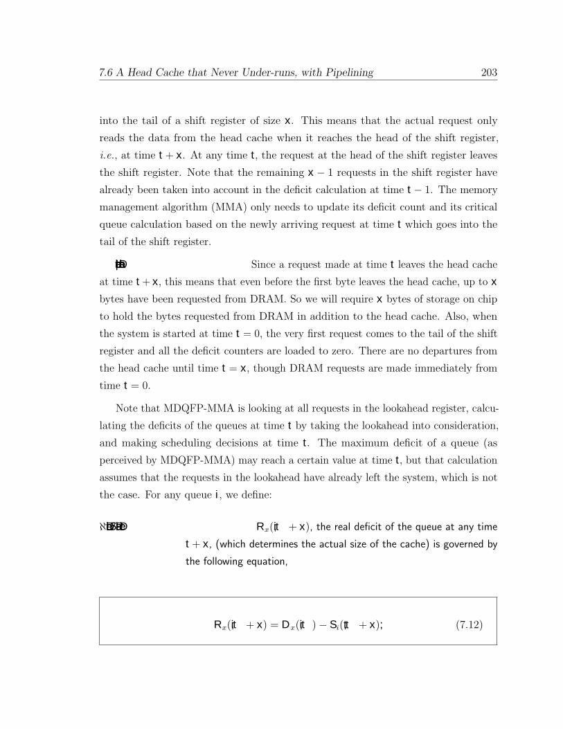
7.6 A Head Cache that Never Under-runs, with Pipelining 203
into the tail of a shift register of size x. This means that the actual request only
reads the data from the head cache when it reaches the head of the shift register,
i.e., at time t+ x. At any time t, the request at the head of the shift register leaves
the shift register. Note that the remaining x− 1 requests in the shift register have
already been taken into account in the deficit calculation at time t− 1. The memory
management algorithm (MMA) only needs to update its deficit count and its critical
queue calculation based on the newly arriving request at time t which goes into the
tail of the shift register.
Implementation Details: Since a request made at time t leaves the head cache
at time t+ x, this means that even before the first byte leaves the head cache, up to x
bytes have been requested from DRAM. So we will require x bytes of storage on chip
to hold the bytes requested from DRAM in addition to the head cache. Also, when
the system is started at time t = 0, the very first request comes to the tail of the shift
register and all the deficit counters are loaded to zero. There are no departures from
the head cache until time t = x, though DRAM requests are made immediately from
time t = 0.
Note that MDQFP-MMA is looking at all requests in the lookahead register, calcu-
lating the deficits of the queues at time t by taking the lookahead into consideration,
and making scheduling decisions at time t. The maximum deficit of a queue (as
perceived by MDQFP-MMA) may reach a certain value at time t, but that calculation
assumes that the requests in the lookahead have already left the system, which is not
the case. For any queue i, we define:
ℵDenition 7.5. Real Decit Rx(i, t+ x), the real deficit of the queue at any time
t+ x, (which determines the actual size of the cache) is governed by
the following equation,
Rx(i, t+ x) = Dx(i, t)− Si(t, t+ x), (7.12)

7.6 A Head Cache that Never Under-runs, with Pipelining 204
where, Si(t, t+x) denotes the number of DRAM services that queue i receives between
time t and t+x, and Dx(i, t) denotes the deficit as perceived by MDQF at time t, after
taking the lookahead requests into account. Note, however, that since Si(t, t+ x) > 0,
if a queue causes a cache miss at time t+ x, that queue would have been critical at
time t. We will use this fact later on in proving the bound on the real size of the head
cache.
Lemma 7.3. (Sufficiency) Under the MDQFP-MMA policy, and a pipeline delay of
x > b time slots, the real deficit of any queue i is bounded for all time t+ x by
Rx(i, t+ x) 6 C = b (2 + ln[Qb/(x− 2b)]) . (7.13)
Proof. See Appendix H. r
This leads to the main result that tells us a cache size that will be sufficient with the
new algorithm.
Theorem 7.4. (Sufficiency) With MDQFP and a pipeline delay of x (where x > b),
the number of bytes that are sufficient to be held in the head cache is
Qw = Q(C + b). (7.14)
Proof. The proof is similar to Theorem 7.3. r
7.6.2 Tradeo between Head SRAM Size and Pipeline Delay
Intuition tells us that if we can tolerate a larger pipeline delay, we should be able to
make the head cache smaller; and that is indeed the case. Note that from Theorem 7.4

7.7 A Dynamically Allocated Head Cache that Never Under-runs 205
the rate of decrease of size of the head cache (and hence the size of the SRAM) is,
∂C
∂x= − 1
x− 2b, (7.15)
which tells us that even a small pipeline will give a big decrease in the size of the
SRAM cache.
Example 7.5. As an example, Figure 7.5 shows the size of the head cache as a
function of the pipeline delay x when Q = 1000 and b = 10 bytes.
With no pipelining, we need 90 kbytes of SRAM, but with a pipeline
of Qb = 10000 time slots, the size drops to 10 kbytes. Even with a
pipeline of 300 time slots (this corresponds to a 60 ns pipeline in a
40 Gb/s line card) we only need approximately 55 kbytes of SRAM: A
small pipeline gives us a much smaller SRAM.12
7.7 A Dynamically Allocated Head Cache that
Never Under-runs, with Large Pipeline Delay
Until now we have assumed that the head cache is statically allocated. Although a
static allocation is easier to maintain than a dynamic allocation (static allocation uses
circular buffers, rather than linked lists), we can expect a dynamic allocation to be
more efficient because it’s unlikely that all the FIFOs will fill up at the same time
in the cache. A dynamic allocation can exploit this to devote all the cache to the
occupied FIFOs.
Let’s see how much smaller we can make the head cache as we dynamically allocate
FIFOs. The basic idea is as follows:
12The “SRAM size vs. pipeline delay” curve is not plotted when the pipeline delay is between1000 and 10,000 time slots since the curve is almost flat in this interval.

7.7 A Dynamically Allocated Head Cache that Never Under-runs 206
Box 7.2: Benets of Buer Caching
The buffer caching algorithms described in this chapter have been developed for anumber of Cisco’s next-generation high-speed Enterprise routers. In addition to scalingrouter performance and making their memory performance robust against adversaries (aswas described in Box 7.1), a number of other advantages have come to light.
1. Reduces Memory Cost: Caches reduce memory cost, as they allow the useof commodity memories such as DRAMs [3] or newly available eDRAM [26], incomparison to specialized memories such as FCRAM [9], RLDRAMs [8], and QDR-SRAMs [2]. In most systems, memory cost (approximately 25%-33% of system cost)is reduced by 50%.
2. Increases Memory Capacity Utilization: The “b-byte” memory blocks ensurethat the cache accesses are always fully utilized. As a consequence, this eliminatesthe “65-byte” problem and leads to better utilization of memory capacity and memorybandwidth. In some cases, the savings can be up to 50% of the memory capacity.
3. Reduces Memory Bandwidth and Lowers Worst-Case Power: A conse-quence of solving the “65-byte” problem is that the memory bandwidth to and fromcache is minimized and is exactly 2R. Statistical packet buffer designs require alarger bandwidth (above 2NR as described in Section 7.8) to alleviate potential bankconflicts. Overall, this has helped reduce memory bandwidth (and worst-case I/Opower) by up to 75% in some cases, due to better bandwidth utilization.
4. Reduces Packet Latency: The packets in a robust cache are always found on-chip. So these caches reduce the latency of packet memory access in a router. Thus,caches have found applications in the low-latency Ethernet [131] and inter-processorcommunication (IPC) markets, which require very low network latency.
5. Enables the Use of Complementary Technologies: The packet-processingASICs on high-speed routers are limited by the number of pins they can interface to.High-speed serialization and I/O technologies [27] can help reduce the number ofmemory interconnect pins,a but they suffer from extremely high latency. The cachescan be increased in size (from the theoretical bounds derived in this chapter) toabsorb additional memory latency, thus enabling these complementary technologies.
6. Enable Zero Packet Drops: A robust cache is sized for adversarial conditions(Box 7.1) and never drops a packet. This feature has found uses in the storagemarket [61], where the protocol mandates zero packet drops on the network.
7. ASIC and Board Cost Savings: As a consequence of the above benefits, thepacket-processing ASICs require less pins, and there are fewer memory devices onthe board, resulting in smaller ASICs and less-complex boards.
At the time of writing, we have implemented the cache in the next generation of Ciscohigh-speed enterprise router products, which span the Ethernet, storage, and inter-processorcommunication markets. The above benefits have collectively made routers more affordable,robust, and practical to build.
aWith today’s technology, a 10Gb/s differential pair serdes gives five times more bandwidthper pin than standard memory interfaces.

7.7 A Dynamically Allocated Head Cache that Never Under-runs 207
0
20
40
60
80
100
0 100 200 300 400 500 600 700 800 900 1000
Siz
e of
SR
AM
(K
Byt
es)
Pipeline Delay (Time Slots)
Approximate closed-form bound
Pipeline Delay (Time Slots)
Size
of S
RA
M (
Kby
tes)
Approximate Closed Form Bound
0 100 200 300 400 500 600 700 800 900 10000
20
60
40
80
100
Figure 7.5: The SRAM size (in bold) as a function of pipeline delay (x). The example isfor 1000 queues (Q = 1000), and a block size of b = 10 bytes.
DIdea. At any time, some queues are closer to becoming critical than others.
The more critical queues need more buffer space, while the less critical queues
need less. When we use a lookahead buffer, we know which queues are close to
becoming critical and which are not. We can therefore dynamically allocate more
space in the cache for the more critical queues, borrowing space from the less
critical queues that don’t need it.
7.7.1 The Smallest Possible Head Cache
Theorem 7.5. (Necessity) For a finite pipeline, the head cache must contain at least
Q(b− 1) bytes for any algorithm.
Proof. Consider the case when the FIFOs in DRAM are all non-empty. If the packet
processor requests one byte from each queue in turn (and makes no more requests),
we might need to retrieve b new bytes from the DRAM for every queue in turn. The
head cache returns one byte to the packet processor and must store the remaining
b− 1 bytes for every queue. Hence the head cache must be at least Q(b− 1) bytes.r

7.7 A Dynamically Allocated Head Cache that Never Under-runs 208
7.7.2 The Earliest Critical Queue First (ECQF) Algorithm
As we will see, ECQF achieves the size of the smallest possible head cache; i.e., no
algorithm can do better than ECQF.
ECQF Algorithm Description: Every time there are b requests to the head
cache, if there are critical queues in the cache, refill the first one to go critical.
Otherwise, do nothing. This is described in detail in Algorithm 7.3.
Note that ECQF (in contrast to MDQFP) never needs to schedule most-deficited
queues. It only needs to wait until a queue becomes critical, and schedule these queues
in order. Also, with ECQF we can delay making requests to replenish a queue from
DRAM until b requests are made to the buffer, instead of making a request every b
time slots. If requests arrive every time slot, the two schemes are the same. However,
if there are empty time slots, this allows ECQF to delay requests, so that the moment
b bytes arrive from DRAM, b bytes also leave the cache, preventing the shared head
cache from ever growing in size beyond Q(b− 1) bytes.
This subtle difference is only of theoretical concern, as it does not affect the
semantics of the algorithm. In the examples that follow, we will assume that requests
arrive every time slot.
Example 7.6. Figure 7.6 shows an example of the ECQF algorithm for Q = 4
and b = 3. Figure 7.6(a) shows that the algorithm (at time t = 0)
determines that queues A,B will become critical at time t = 6 and
t = 8, respectively. Since A goes critical sooner, it is refilled. Bytes
from queues A,B,C are read from the head cache at times t = 0, 1, 2.
In Figure 7.6(b), B goes critical first and is refilled. Bytes from queues
D,A,B leave the head cache at times t = 3, 4, 5. The occupancy of
the head cache at time t = 6 is shown in Figure 7.6(c). Queue A is
the earliest critical queue (again) and is refilled.

7.7 A Dynamically Allocated Head Cache that Never Under-runs 209
A1 C1A2 C2B1 D1B2 D2
Head Cache
Requests in Lookahead
(a) State at t=0
Q(A,0) = 2; Q(A,6) critical.Q(B,0) = 2; Q(B,8) critical.Queue A is requested
A3 A4A2 C2A5 D1B2 D2
A3 A4B4 C2A5 B3B5 D2
Requests in Lookahead
From DRAM
Head Cache
Head Cache
Requests in Lookahead
Returned Data
Returned Data
From DRAM
(b) State at t=3
Q(A,3) = 4; Q(A,11) critical.Q(B,3) = 1; Q(B,9) critical.Bytes A3,A4,A5 arrive
(c) State at t=6
Q(A,6) = 3; Q(A, 11) critical.Q(C,6) = 2; Q(C,13) critical.Bytes B3,B4,B5 arrive.Queue A is requested.
B23A2 D1 B1 C1 A1
B3A1 C1 B1 D1 A2 B2 A3 A4
C2D1 A2 B2 A3 A4 B3 A5 A6
B1 C1 A1
A8A3 A4 B3 A5 A6 C2 C3 A7
Queue B requested
Figure 7.6: ECQF with Q = 4 and b = 3 bytes. The dynamically allocated head cache is 8bytes and the lookahead buffer is Q(b− 1) + 1 = 9 bytes.

7.7 A Dynamically Allocated Head Cache that Never Under-runs 210
Algorithm 7.3: The earliest critical queue first algorithm.
input : Queue occupancy and requests in pipeline (shift register) lookahead.1
output: The queue to be replenished.2
/* Wait for b requests, rather than b time slots */3
/* Ensure critical queues are not fetched “too early" ˜4
/* Hence, delay replenishment if empty request time slots5
*/
/* Calculate queue to replenish */6
repeat every b time slots for every b requests encountered7
CurrentQueues ← (1, 2, . . . , Q)8
/* Calculate earliest critical queue if it exists */9
/* By design it will have space to accept data in cache10
*/
QECritical ← FindEarliestCriticalQueue(CurrentQueues)11
if ∃ QECritical then12
Replenish(QECritical)13
UpdateDeficit(QECritical)14
/* Register request for a queue */15
repeat every time slot16
if ∃ request for q then17
UpdateDeficit(q)18
PushShiftRegister(q)19
/* Service request for a queue, Qb time slots later */20
repeat every time slot21
q ← PopShiftRegister()22
if ∃ q then23
ReadData(q)24
To figure out how big the head cache needs to be, we will make three simplifying
assumptions (described in Appendix H) that help prove a lower bound on the size of
the head cache. We will then relax the assumptions to prove the head cache need
never be larger than Q(b− 1) bytes.

7.8 Implementation Considerations 211
Theorem 7.6. (Sufficiency) If the head cache has Q(b − 1) bytes and a lookahead
buffer of Q(b− 1) + 1 bytes (and hence a pipeline of Q(b− 1) + 1 slots), then ECQF
will make sure that no queue ever under-runs.
Proof. See Appendix H. r
7.8 Implementation Considerations
1. Complexity of the algorithms: All of the algorithms require deficit counters;
MDQF and MDQFP must identify the queue with the maximum deficit every
b time slots. While this is possible to implement for a small number of queues
using dedicated hardware, or perhaps using a heap data structure [146], it may
not scale when the number of queues is very large. The other possibility is to use
calendar queues, with buckets to store queues with the same deficit. In contrast,
ECQF is simpler to implement. It only needs to identify when a deficit counter
becomes critical, and replenish the corresponding queue.
2. Reducing b: The cache scales linearly with b, which scales with line rates.
It is possible to use ping-pong buffering [147] to reduce b by a factor of two
(from b = 2RT to b = RT ). Memory is divided into two equal groups, and a
block is written to just one group. Each time slot, blocks are read as before.
This constrains us to write new blocks into the other group. Since each group
individually caters a read request or a write request per time slot, the memory
bandwidth of each group needs to be no more than the read (or write) rate R.
Hence block size, b = RT . However, as soon as either one of the groups becomes
full, the buffer cannot be used. So in the worst case, only half of the memory
capacity is usable.
3. Saving External Memory Capacity and Bandwidth: One consequence of
integrating the SRAM into the packet processor is that it solves the so-called
“65 byte problem”. It is common for packet processors to segment packets into
fixed-size chunks, to make them easier to manage, and to simply the switch
fabric; 64 bytes is a common choice because it is the first power of two larger

7.9 Summary of Results 212
Table 7.1: Tradeoffs for the size of the head cache.
Head SRAMPipeline Delay
(time slot)
Head SRAM(bytes, type, algorithm)
Source
0 Qb(3 + ln Q), Static, MDQF Theorem 7.3x Qb(3 + ln[Qb=(x− 2b)]), Static, MDQFP Theorem 7.4
Q(b− 1) + 1 Q(b− 1), Dynamic, ECQF Theorem 7.6
Table 7.2: Tradeoffs for the size of the tail cache.
Tail SRAM(bytes, type, algorithm)
Source
Qb(3 + ln Q), Static, MDQF By a symmetry argument to Theorem 7.3Qb, Dynamic Refer to Theorem 7.1
than the size of a minimum-length IP datagram. But although the memory
interface is optimized for 64-byte chunks, in the worst case it must be able to
handle a sustained stream of 65-byte packets – which will fill one chunk, while
leaving the next one almost empty. To overcome this problem, the memory
hierarchy is almost always run at twice the line rate: i.e., 4R , which adds to the
area, cost, and power of the solution. Our solution doesn’t require this speedup
of two. This is because data is always written to DRAM in blocks of size b,
regardless of the packet size. Partially filled blocks in SRAM are held on chip,
are never written to DRAM, and are sent to the head cache directly if requested
by the head cache. We have demonstrated implementations of packet buffers
that run at 2R and have no fragmentation problems in external memory.
7.9 Summary of Results
Table 7.1 compares various cache sizes with and without pipelining, for static and
dynamic allocation. Table 7.2 compares the various tail cache sizes when implemented
using a static or dynamic tail cache.

7.10 Related Work 213
7.10 Related Work
Packet buffers based on a SRAM-DRAM hierarchy are not new, and although not
published before, have been deployed in commercial switches and routers. However,
there is no literature that describes or analyzes the technique. We have found that
existing designs are based on ad-hoc statistical assumptions without hard guarantees.
We divide the previously published work into two categories:
Systems that give statistical performance: In these systems, the memory
hierarchy only gives statistical guarantees for the time to access a packet, similar
to interleaving or pre-fetching used in computer systems [148, 149, 150, 151, 152].
Examples of implementations that use commercially available DRAM controllers
are [153, 154]. A simple technique to obtain high throughputs using DRAMs (using
only random accesses) is to stripe a packet13 across multiple DRAMs [138]. In this
approach, each incoming packet is split into smaller segments, and each segment is
written into different DRAM banks; the banks reside in a number of parallel DRAMs.
With this approach, the random access time is still the bottleneck. To decrease the
access rate to each DRAM, packet interleaving can be used [147, 155]; consecutive
arriving packets are written into different DRAM banks. However, when we write
the packets into the buffer, we don’t know the order they will depart; and so it can
happen that consecutive departing packets reside in the same DRAM row or bank,
causing row or bank conflicts and momentary loss in throughput. There are other
techniques that give statistical guarantees, where a memory management algorithm
(MMA) is designed so that the probability of DRAM row or bank conflicts is reduced.
These include designs that randomly select memory locations [156, 157, 139, 140], so
that the probability of row or bank conflicts in DRAMs is considerably reduced. Using
a similar interleaved memory architectures, the authors in [158] analyze the packet
drop probability, but make assumptions about packet arrival patterns.
Under certain conditions, statistical bounds (such as average delay) can be found.
While statistical guarantees might be acceptable for a computer system (in which we
13This is sometimes referred to as bit striping.
7.10 Related Work 214
are used to cache misses, TLB misses, and memory refresh), they are not generally
acceptable in a router, where pipelines are deep and throughput is paramount.
Systems that give deterministic worst-case performance guarantees:
There is a body of work in [159, 160, 161, 162, 163] that analyzes the performance
of a queueing system under a model in which variable-size packet data arrives from
N input channels and is buffered temporarily in an input buffer. A server reads
from the input buffer, with the constraint that it must serve complete packets from a
channel. In [161, 162] the authors consider round robin service policies, while in [163]
the authors analyze an FCFS server. In [159] an optimal service policy is described,
but this assumes knowledge of the arrival process. The most relevant previous work
is in [160], where the authors in their seminal work analyze a server that serves the
channel with the largest buffer occupancy, and prove that under the above model the
buffer occupancy for any channel is no more than L(2 + ln(N − 1)), where L is the
size of the maximum-sized packet.
7.10.1 Comparison of Related Work
Our work on packet buffer design was first described in [164, 165], and a complete
version of the paper appears in [166, 167]. Subsequent to our work, a similar problem
with an identical service policy has also been analyzed in [168, 169, 170], where the
authors show that servicing the longest queue results in a competitive ratio of ln(N)
compared to the ideal service policy, which is offline and has knowledge of all inputs.
Our work has some similarities with the papers above. However, our work differs in
the following ways. First, we are concerned with the size of two different buffer caches,
the tail cache and a head cache, and the interaction between them. We show that the
size of the tail cache does not have a logarithmic dependency, unlike [160, 168, 169, 170],
since this cache can be dynamically shared among all arriving packets at the tails of
the queues. Second, the size of our caches is independent of L, the maximum packet
size, because unlike the systems in [159, 160, 161], our buffer cache architecture can
store data in external memory. Third, we obtain a more general bound by analyzing
the effect of pipeline latency x on the cache size. Fourth, unlike the work done

7.11 Conclusion 215
in [168, 169, 170] which derives a bound on the competitive ratio with an ideal server,
we are concerned with the actual size of the buffer cache at any given time (since this
is constrained by hardware limitations).
7.10.2 Subsequent Work
In subsequent work, the authors in [171], use the techniques presented here to build
high-speed packet buffers. Also, subsequent to our work, the authors in [172] analyze
the performance of our caching algorithm when it is sized smaller than the bounds
that are derived in this chapter. Similar to the goal in [172], we have considered
cache size optimizations in the absence of adversarial patterns.14 Unsurprisingly, when
adversarial patterns are eliminated, the cache sizes can be reduced significantly, in
some cases up to 50%.
The techniques that we have described in this chapter pertain to the packet-by-
packet operations that need to be performed for building high-speed packet buffers,
on router line cards. We do not address the buffer management policies, which control
how the buffers are allocated and shared between the different queues. The reader is
refereed to [173, 174] for a survey of a number of existing techniques.
7.11 Conclusion
Packet switches, regardless of their architecture, require packet buffers. The general
architecture presented here can be used to build high-bandwidth packet buffers for any
traffic arrival pattern or packet scheduling algorithm. The scheme uses a number of
DRAMs in parallel, all controlled from a single address bus. The costs of the technique
are: (1) a (presumably on-chip) SRAM cache that grows in size linearly with line rate
and the number of queues, and decreases with an increase in the pipeline delay, (2) a
lookahead buffer (if any) to hold requests, and (3) a choice of memory management
algorithms that must be implemented in hardware.
14We have encountered designs where the arbiter is benign, reads in constant-size blocks, or requestspackets in a fixed round robin (or weighted round robin) pattern, for which such optimizations canbe made.

7.11 Conclusion 216
Example 7.7. As an example of how these results are used, consider a typical 48-
port commercial gigabit Ethernet switching line card that uses SRAM
for packet buffering.15 There are four 12G MAC chips on board, each
handling 12 ports. Each Ethernet MAC chip stores 8 transmit and
3 receive ports per 1G port, for a total of 132 queues per MAC chip.
Each MAC chip uses 128 Mbits of SRAM. With today’s memory prices,
the SRAM costs approximately $128 (list price). With four Ethernet
MACs per card, the total memory cost on the line card is $512 per
line card. If the buffer uses DRAMs instead (assume 16-bit wide data
bus, 400 MHz DDR, and a random access time of T = 51.2 ns), up
to 64 bytes16 can be written to each memory per 51.2-ns time slot.
Conservatively, it would require 6 DRAMs (for memory bandwidth),
which cost (today) about $144 for the line card. With b = 384 bytes,
the total cache size would be ∼3.65 Mb, which is less than 5% of the
die area of most packet processing ASICs today. Our example serves
to illustrate that significant cost savings are possible.
While there are systems for which this technique is inapplicable (e.g., systems for
which the number of queues is too large, or where the line rate requires too large
a value for b, so that the SRAM cannot be placed on chip), our experience with
enabling this technology at Cisco Systems shows that caching is practical, and we have
implemented it in fast silicon. It has been broadly applied for the next generation
of many segments of the enterprise market [4, 176, 177, 178]. It is also applicable to
some segments of the edge router market [179] and some segments of the core router
market [180], where the numbers of queues are in the low hundreds.
We have also modified this technique for use in VOQ buffering [181] and stor-
age [182] applications. Our techniques have also paved the way for the use of comple-
mentary high-speed interconnect and memory serialization technologies [32], since the
caches hide the memory latency of these beneficial serial interconnect technologies,
15Our example is from Cisco Systems [175].16It is common in practice to write data in sizes of 64 bytes internally, as this is the first power of
2 above the sizes of ATM cells and minimum-length TCP segments (40 bytes).

7.11 Conclusion 217
enabling them to be used for networking. We estimate that a combination of caching
and complementary serial link technologies has resulted in reducing memory power by
a factor of ∼25-50% [31]). It has also made routers more affordable (by reducing yearly
memory costs at Cisco Systems by > $100M [33] for packet buffering applications
alone), and has helped reduce the physical area to build high-speed routers by ∼50%.
We estimate that more than 1.5 M instances of packet buffering-related (on over seven
unique product instances) caching technologies will be made available annually, as
Cisco Systems proliferates its next generation of high-speed Ethernet switches and
Enterprise routers.
In summary, the above techniques can be used to build extremely cost-efficient
and robust packet buffers that: (1) give the performance of SRAM with the capacity
characteristics of a DRAM, (2) are faster than any that are commercially available
today, and, (3) enable packet buffers to be built for several generations of technology to
come. As a result, we believe that we have fundamentally changed the way high-speed
switches and routers use external memory.
Summary
1. Internet routers and Ethernet switches contain packet buffers to hold packets during times
of congestion. Packet buffers are at the heart of all packet switches and routers, which
have a combined annual market of tens of billions of dollars, with equipment vendors
spending hundreds of millions of dollars yearly on memory.
2. We estimate [24, 33] that packet buffers are alone responsible for almost 40% of all
memory consumed by high-speed switches and routers today.
3. Designing packet buffers was formerly easy: DRAM was cheap, low-power, and widely
used. But something happened at 10 Gb/s, when packets began to arrive and depart
faster than the access time of a DRAM. Alternative memories were needed; but SRAM is
too expensive and power-hungry.
4. A caching solution is appealing, with a hierarchy of SRAM and DRAM, as used by the
computer industry. However, in switches and routers, it is not acceptable to have a
“miss-rate”, as it reduces throughput and breaks pipelines.
5. In this chapter, we describe how to build caches with 100% hit-rate under all conditions,

7.11 Conclusion 218
by exploiting the fact that switches and routers always store data in FIFO queues. We
describe a number of different ways to do this, with and without pipelining, with static or
dynamic allocation of memory.
6. In each case, we prove a lower bound on how big the cache needs to be, and propose an
algorithm that meets, or comes close to, the lower bound.
7. The main result of this chapter is that a packet buffer cache with Θ(Qb ln Q) bytes is
sufficient to ensure that the cache has a 100% hit rate — where Q is the number of FIFO
queues, and b is the memory block size (Theorem 7.3).
8. We then describe techniques to reduce the cache size. We exploit the fact that ASICs
have deep pipelines, and so allow for packets to be streamed out of the buffer with a
pipeline delay of x time slots.
9. We show that there is a well-defined continuous tradeoff between (statically allocated)
cache size and pipeline delay, and that the cache size is proportional to Θ(Qb ln[Qb=x])
(Theorem 7.4).
10. If the head cache is dynamically allocated, its size can be further reduced to Qb bytes if
an ASIC can tolerate a large pipeline delay (Theorem 7.6).
11. These techniques are practical, and have been implemented in fast silicon in multiple
high-speed Ethernet switches and Enterprise routers.
12. Our techniques are resistant to adversarial patterns that can be created by hackers or
viruses. We show that the memory performance of the buffer can never be compromised,
either now or, provably, ever in future.
13. As a result, the performance of a packet buffer is no longer dependent on the speed of a
memory, and these techniques have fundamentally changed the way switches and routers
use external memory.

Chapter 8: Designing Packet Schedulers from
Slower MemoriesMay 2008, Stateline, NV
Contents
8.1 Introduction . . . . . . . . . . . . . . . . . . . . . . . . . . . . . . . . 221
8.1.1 Background . . . . . . . . . . . . . . . . . . . . . . . . . . . . . . . . . 222
8.1.2 Where Are Schedulers Used Today? . . . . . . . . . . . . . . . . . . . 224
8.1.3 Problem Statement . . . . . . . . . . . . . . . . . . . . . . . . . . . . . 226
8.1.4 Goal . . . . . . . . . . . . . . . . . . . . . . . . . . . . . . . . . . . . . 227
8.1.5 Organization . . . . . . . . . . . . . . . . . . . . . . . . . . . . . . . . 228
8.2 Architecture of a Typical Packet Scheduler . . . . . . . . . . . . . . 229
8.3 A Scheduler Hierarchy for a Typical Packet Scheduler . . . . . . . 232
8.4 A Scheduler that Operates With a Buffer Hierarchy . . . . . . . . 236
8.5 A Scheduler Hierarchy that Operates With a Buffer Hierarchy . . 238
8.6 A Scheduler that Piggybacks on the Buffer Hierarchy . . . . . . . 240
8.6.1 Architecture of a Piggybacked Scheduler . . . . . . . . . . . . . . . . . 241
8.6.2 Interaction between the Packet Buffer and Scheduler Cache . . . . . . 243
8.6.3 A Work-conserving Packet Scheduler . . . . . . . . . . . . . . . . . . . 249
8.7 Design Options and Considerations . . . . . . . . . . . . . . . . . . 250
8.8 Conclusion . . . . . . . . . . . . . . . . . . . . . . . . . . . . . . . . . 252
List of Dependencies
• Background: The memory access time problem for routers is described in
Chapter 1. Section 1.5.3 describes the use of caching techniques to alleviate
memory access time problems for routers in general.

Additional Readings
• Related Chapters: The caching hierarchy described in this chapter was first
examined in Chapter 7 with respect to implementing high-speed packet buffers.
The present discussion uses results from Sections 7.5 and 7.6. A similar technique
is used in Chapter 9 to implement high-speed statistics counters.
Table: List of Symbols.
b Memory Block Sizec, C CellD Descriptor SizeL Latency between Scheduler Request and Buffer Response
Pmin Minimum Packet SizePmax Maximum Packet Size
Q Number of Linked Lists, QueuesR Line RateT Time Slot
TRC Random Cycle Time of Memory
Table: List of Abbreviations.
DRAM Dynamic Random Access MemoryMMA Memory Management AlgorithmMDQF Most Deficited Queue FirstMDLLF Most Deficited Linked List FirstDRAM Dynamic Random Access MemorySRAM Static Random Access Memory
“You say shed-ule, I say sked-ule,
You like shed-ule, I like best effort!”
— The Great QoS Debate† 8Designing Packet Schedulers from Slower
Memories
8.1 Introduction
Historically, communication networks (e.g., telephone and ATM networks) were pre-
dominantly circuit-switched. When end hosts wanted to communicate, they would
request the network to create a fixed-bandwidth channel (“circuit”) between the source
and destination. The connection could request assurances on bandwidth, as well as
bounded delay and jitter. If the network had the resources to accept the request, it
would reserve the circuit for the connection, and allow the end hosts to communicate
in an isolated environment.
In contrast, as described in Chapter 7, the Internet today is packet switched. Hosts
communicate by sending a stream of packets, and may join or leave without explicit
permission from the network. Packets between communicating hosts are statistically
multiplexed across the network, and share network and router resources (e.g., links,
routers, buffers, etc.). If the packet switched network infrastructure operated in such
a rudimentary manner, then no guarantees could be provided, and only best-effort
service could be supported.
†A riff on the immortal line, “You like tomayto, I like tomahto”, from the Ira and George Gershwinsong “Let’s Call the Whole Thing Off”.
221

8.1 Introduction 222
The purpose of this chapter is not to debate the merits of circuit vs. packet
switched networks.1 Rather, we are motivated by the following question: How can
a router in today’s predominantly packet switched environment differentiate between,
provide network resources for, and satisfy the demands of varied connections? More
specifically, how can a high-speed router perform this task at wire-speeds?
8.1.1 Background
The Internet today can support a wide variety of applications and their unique
performance requirements, because network and router infrastructures identify and
differentiate between packets and provide them appropriate qualities of service. The
different tiers of service are overlaid on top of a (usually over-provisioned) best-effort
IP network.
Example 8.1. For example, IPTV [29] places strict demands on the bandwidth
provided; VoIP, telnet, remote login, and inter-processor communica-
tion require very low latency; videoconferencing and Telepresence [28]
require assurances on bandwidth, worst-case delay, and worst-case jitter
characteristics from the network; and storage protocols mandate no
packet drops. Box 8.2 provides a historical perspective, with further
examples of the many applications currently supported on the Internet.
In order to provide different qualities of service, routers perform four tasks:
1. Identify ows via packet classication: First, packets belonging to different
applications or protocols that need different tiers of service are identified via
packet classification. Packet classification involves comparing packet headers
against a set of known rules (“classifiers”) so that the characteristics of the
communication, i.e., the application type, source, destination characteristics,
and transport protocol, etc., can be identified. Classification is an algorithmically
intensive task. Many algorithms for packet classification have been proposed: for
1The reader is referred to [183] for a detailed discussion and comparison of the two kinds ofnetworks.

8.1 Introduction 223
example, route lookup algorithms [134] classify packets based on their source or
destination characteristics; and flow classification algorithms [184] are protocol
and application aware, and are used to more finely identify individual connections
(commonly referred to as flows). Some routers can also perform deep packet
classification [185].
2. Isolate and buer ows into separate queues: Once these flows are classi-
fied, they need to be isolated from each other, so that their access to network
and router resources can be controlled. This is done by buffering them into
separate queues. Depending on the granularity of the classifier, and the number
of queues maintained by the packet buffer, one or more flows may share a queue
in the buffer. Packet buffering is a memory-intensive task, and we described a
caching hierarchy in Chapter 7 to scale the performance of packet buffering.
3. Maintain scheduling information for each queue: Once the packets for a
particular flow are buffered to separate queues, a scheduler or memory manager
maintains “descriptors” for all the packets in the queues. The descriptors keep
information such as the length and location of all packets in the queue. In
addition, the scheduler maintains the order of packets by linking the descriptors
for the consecutive packets that are destined to a particular queue.2 The scheduler
makes all of this information available to an arbiter, and is also responsible for
responding to the arbiter’s requests, as described below.
4. Arbitrate ows based on network policy:Arbitration is the task of imple-
menting network policy, i.e., allocating resources (such as share of bandwidth,
order in which the queues are serviced, distinguishing queues into different
priority levels, etc.) among the different queues. The arbiter has access to the
scheduler linked lists (and so is made aware of the state of all packets in the
queues) and other queue statistics maintained by the scheduler. Based on a
programmed network policy, it requests packets in a specific order from the
different queues. A number of arbitration algorithms have been proposed to
implement the network policy. These include weighted fair queueing [17] and its
2The scheduler may also keep some overall statistics, e.g., the total occupancy of the queue, thetotal occupancy for a group of queues (which may be destined to the same output port), etc.

8.1 Introduction 224
variants, such as GPS [18], Virtual Clock [19], and DRR [20]. Other examples
include strict priority queueing and WF2Q [21]. A survey of existing arbitration
policies and algorithms is available in [186].3
8.1.2 Where Are Schedulers Used Today?
Broadly speaking, a scheduler is required wherever packets are stored in a buffer and
those packets need to be differentiated when they access network resources.
NObservation 8.1. A buffer (which stores packet data), a scheduler (which keeps
descriptors to packet data so that it can be retrieved), and an arbiter
(which decides when to read packets and the order in which they are
read) always go together.
Figure 8.1 shows an example of a router line card where scheduling information is
needed by the arbiter (to implement network policy) in four instances:
1. On the ingress line card, an arbiter serves the ports in the ingress MAC in
different ratios, based on their line rates and customer policy.
2. Later, packets are buffered in separate virtual output queues (VOQs), and a
central switch arbiter requests packets from these VOQs (based on the switch
fabric architecture and the matching algorithms that it implements).
3. On the egress line card, the output manager ASIC re-orders packets that arrive
from a switch fabric (that may potentially mis-order packets).
4. Finally, when packets are ready to be sent out, an arbiter in the egress MAC serves
the output ports based on their line rates and quality of service requirements.
It is interesting to compare Figure 7.1 with Figure 8.1. The two diagrams are
almost identical, and a scheduler is required in every instance where there is a buffer.
3In previous literature, the arbitration algorithms have also been referred to as “QoS scheduling”algorithms. In what follows, we deliberately distinguish the two terms: arbitration is used to specifyand implement network policy, and scheduling is used to provide the memory management informationneeded to facilitate the actions of an arbiter.

8.1 Introduction 225
Multi-path
Egress Line Card
MAC
(1) Scheduling for
VOQ M
anagerM
AC O
utpu
t Mul
ticas
t
Man
ager
Rep
licat
or
Ingress Line Card
Slow
Gateway
for QoS and (4) Egress Scheduling for
..
R’
r << R/10
R’R’
sR
sR sRWAN
Switch Fabric
1 4 2
Mis-ordered Cells
customer policy
r
sR
Speedup
A1
..
R’
R’R’R’
A2
Z1
Z2
Z3
B1
..
A1AN A2B1BN B2
Z1ZN Z2
....
..
A4 A3 Z1 B1 A2 A1
A3A4
Z2 B2
.. A3B3
Z3
..
A1B1A2Z2
A3A4
..
..
.. Z1
B2
Arbitration Ratio: 2:1:3: ... 1
Arbitration based on fabric
Arbiter Central
Z2 A3 A2 B1 A1
(2) Scheduling for fabric contention
Remote Lookup Unit
..
A1 B1H1 J2
P3 Q4
..
..
..X1
R2
Arbitration Ratio: 10:5:2 ... :1
P3 Q4 R2
(3) Scheduling
port speed mismatch
after re-ordering
364... 969016
60101
40
70
1194001101
...40
...
Descriptors
1... 2 4
79
11
11
121415
...12
...
3
s 1≥
Figure 8.1: Scheduling in Internet routers.

8.1 Introduction 226
The only exception is the case where the buffer is a single first in first out (FIFO)
queue, as in the lookup latency buffer and the multicast replication buffer in Figure 7.1.
If there is only a single queue, it is trivial for a scheduler to maintain descriptors. Also,
the FIFO policy is trivial to implement, and no arbiter is required.
8.1.3 Problem Statement
As far as we know, contrary to the other tasks described above, the task of maintaining
the scheduler database, which involves maintaining and managing descriptor linked
lists in memory, has not been studied before. We are particularly interested in this
task, as it is a bottleneck in building high-speed router line cards, since:
1. It places huge demands on the memory access rate, and
2. It requires a large memory capacity (similar to packet buffers), and so cannot
always be placed on-chip.
As we saw earlier, the scheduler and arbiter operate in unison with a packet buffer.
Thus, the scheduler must enqueue and dequeue descriptors for packets at the rate at
which they arrive and leave the buffer, i.e., R. In the worst case, this needs to be
done in the time that it takes for the smallest-size packet to arrive.
In some cases, the scheduler may also have to operate faster than the line rate.
This happens because packets themselves may arrive to the buffer faster than the line
rate (e.g., due to speedup in the fabric). Another reason is that the buffer may need
to support multicast packets at high line rates, for which multiple descriptors (one
per queue to which the multicast packet is destined) need to be created per packet.
Example 8.2. At 10 Gb/s, a 40-byte packet arrives in 32 ns, which means that the
scheduler needs to enqueue and dequeue a descriptor at least once every
32 ns, which is faster than the access rate of commercial DRAM [3].
If a sustained burst of multicast packets (each destined to, say, four
ports) arrives, the scheduler will need to enqueue descriptors every 8 ns
and dequeue descriptors every 32 ns, making the problem much harder.

8.1 Introduction 227
Indeed, as the above example shows, the performance of the scheduler is a significant
bottleneck to scaling the performance of high-speed routers. The memory access rate
problem is at least as hard as the packet buffering problem that we encountered in
Chapter 7 (and sometimes harder, when a large number of multicast packets must be
supported at line rates).
NObservation 8.2. The smallest-size packet on most networks today is ∼40 bytes.4
Note that if the minimum packet size was larger, the scheduler would
have more time to enqueue and dequeue these descriptors. However, the
size of the smallest packet will not change anytime soon — applications
keep their packet sizes small to minimize network latency. For example,
telnet, remote login, and NetMeeting are known to send information
about a keystroke or a mouse click immediately, i.e., no more than one
or two bytes of information at a time.5
8.1.4 Goal
Our goal in this thesis is to enable high-speed routers to provide deterministic per-
formance guarantees, as described in Chapter 1. If the scheduler (which maintains
information about each packet in the router) cannot provide the location of a packet
in a deterministic manner, then obviously the router itself would be unable to give
deterministic guarantees on packet performance! So we will mandate that the sched-
uler give deterministic performance; and similar to our discussion on building robust
routers (see Box 7.1), we will mandate that the scheduler’s performance cannot be
compromised by an adversary.
4Packets smaller than 40 bytes are sometimes created within routers for control purposes. Theseare usually created for facilitating communication within the router itself. They are produced andconsumed at a very low rate. We ignore such packets in the rest of this chapter.
5After encapsulating this information into various physical, link layer, and transport protocolformats to facilitate transfer of the packet over the network, this is approximately ∼40 bytes.

8.1 Introduction 228
8.1.5 Organization
The rest of this chapter is organized as follows: We will describe five different imple-
mentations for a packet scheduler [187] in sections 8.2-8.6:
Method 1. A Typical Packet Scheduler: In Section 8.2, we will describe the
architecture of a typical packet scheduler. We will see that the size
of the descriptor that needs to be maintained by a typical scheduler
can be large, and even comparable in size to the packet buffer that
it manages. And so, the memory for the scheduler will have a large
capacity and require a high access rate.
Method 2. A Scheduler Hierarchy for a Typical Packet Scheduler: In Sec-
tion 8.3, we will show how we can re-use the techniques described in
Chapter 7 to build a caching hierarchy for a packet scheduler. This will
allow us to build schedulers with slower commodity memory, and also
reduce the size of the scheduler memory.
Method 3. A Scheduler that Operates with a Buffer Hierarchy: In Section 8.4,
we show that the amount of information that a scheduler needs to
maintain can be further reduced, if the packet buffer that it operates
with is implemented using the buffer caching hierarchy described in the
previous chapter.
Method 4. A Scheduler Hierarchy that Operates with a Buffer Hierarchy:
As a consequence of using a buffer cache hierarchy, we will show in
Section 8.5 that the size of the scheduler cache also decreases in size
compared to the cache size in Section 8.3.
Method 5. A Scheduler that Piggybacks on the Buffer Hierarchy: Finally, in
Section 8.6 we will present the main idea of this chapter, i.e., a unified
technique where the scheduler piggybacks on the operations of the

8.2 Architecture of a Typical Packet Scheduler 229
packet buffer. With this piggybacking technique, we will completely
eliminate the need to maintain a separate data structure for packet
schedulers.
In Section 8.7, we summarize the five different techniques to build a high-speed
packet scheduler, and discuss where they are applicable, and their different tradeoffs.
Why do we not use just one common technique to build schedulers? We will see in
Section 8.7 that there is no one optimal solution for all scheduler implementations.
Each of the five different techniques that we describe here is optimal based on the
system constraints and product requirements faced when designing a router. Besides,
we will see that in some cases one or more of the above techniques may be inapplicable
for a specific instance of a router.
8.2 Architecture of a Typical Packet Scheduler
A typical scheduler maintains a data structure to link packets destined to separate
queues. If there are Q queues in the system, the scheduler maintains Q separate
linked lists. Each entry in the linked list has a “descriptor” that stores the length of a
particular packet, the memory location for that packet, and a link or pointer to the
next descriptor in that queue; hence the data structure is referred to as descriptor
linked lists. This is shown in Figure 8.2.
When a packet arrives, first it is classified, and the queue that it is destined to is
identified. The packet is then sent to the packet buffer. A descriptor is created which
stores the length of the packet and a pointer to its memory location in the buffer.
This descriptor is then linked to the tail of the descriptor linked list for that queue.
Example 8.3. As shown in Figure 8.2, the descriptor for packet a1 stores the
length of the packet and points to the memory address for packet a1.
Similarly, the descriptor for an arriving packet is written to the tail of
the descriptor queue numbered two.

8.2 Architecture of a Typical Packet Scheduler 230
....
a1
..
a5
..a3
..
a4
z2
z1
b1
Mem 1 Mem 2 Mem 3 Mem k
b3
Packet Data
1
Q
...
2 Arbiter
R 40
Arriving Cell
(1) Write
Packet Descriptors
(4) ReadR64
Departing Cell
(3) Request(2) Descriptor
64, a196, a2
60, b1101, b2
... 40, z1119, z2
90, a3
40, b3
50, z3
(Pointer and Length)
W R
Memory Controller
...
Figure 8.2: The architecture of a typical packet scheduler.

8.2 Architecture of a Typical Packet Scheduler 231
The scheduler makes the descriptor linked lists available to the arbiter. The arbiter
may request head-of-line packets from these descriptor linked lists, in any order based
on its network policy. When this request arrives, the scheduler must dequeue the
descriptor corresponding to the packet, retrieve the packet’s length and memory
location, and request the corresponding number of bytes from the corresponding
address in the packet buffer.
How much memory capacity does a scheduler need? The scheduler maintains
the length and address of a packet in the descriptor. In addition, every descriptor
must keep a pointer to the next descriptor. We can calculate the size of the descriptors
as follows:
1. The maximum packet size in most networks today is 9016 bytes (colloquially
referred to as a jumbo packet). So packet lengths can be encoded in dlog29016e =
13 bits. If the memory data is byte aligned (as is the case with most memories),
this would require 2 bytes.6
2. The size of the packet memory address depends on the total size of the packet
buffer. We will assume that they are 4 bytes each. This is sufficient to store 232
addresses, which is sufficient for a 4 GB packet buffer, and is plenty for most
networks today.
3. Since there is one descriptor per packet, the size of the pointer to the next
descriptor is also 4 bytes long.
So we need approximately 10 bytes per packet descriptor. In the worst case, if
all packets were 40 bytes long, the scheduler would maintain 10 bytes of descriptor
information for every 40-byte packet in the buffer, and so the scheduler database
would be roughly ∼ 14
ththe size of the buffer.
Example 8.4. For example, on a 100 Gb/s link with a 10 ms packet buffer, a
scheduler database that stores a 10-byte descriptor for each 40-byte
6This is also sufficient to encode the lengths of so-called super jumbo packets (64 Kb long) whichsome networks can support. Note that IPv6 also supports an option to create jumbograms whoselength can be up to 4 GB long. If such packets become common, then the length field will need to be4 bytes long.

8.3 A Scheduler Hierarchy for a Typical Packet Scheduler 232
packet would need 250 Mb of memory, and this memory would need to
be accessed every 2.5 ns. The capacity required is beyond the practical
capability of embedded SRAM. Using currently available 36 Mb QDR-
SRAMs,7 this would require 8 external QDR-SRAMs, and over $200 in
memory cost alone!
Because of the large memory capacity and high access rates required by the
scheduler, high-speed routers today keep the descriptors in expensive high-speed
SRAM [2]. It is easy to see how the memory requirements of the scheduler are a
bottleneck as routers scale to even higher speeds. In what follows, we describe various
techniques to alleviate this problem. We begin by describing a caching hierarchy
similar to the one described in Chapter 7.
8.3 A Scheduler Hierarchy for a Typical Packet
Scheduler
NObservation 8.3. An arbiter can dequeue the descriptors for packets in any order
among the different linked lists maintained by the scheduler. However,
within a linked list, the arbiter can only request descriptors for packets
from the head of line. Similarly, when a packet arrives to a queue in
the buffer, the descriptor for the packet is added to the tail of the
descriptor linked list. So the descriptor linked lists maintained by the
scheduler behave similarly to a FIFO queue.
In Chapter 7, we described a caching hierarchy that could be used to implement
high-speed FIFO queues. Based on the observation above, we can implement the
scheduler linked lists with an identical caching hierarchy. Figure 8.3 describes an
example of such an implementation. In what follows, we give a short description of the
scheduler memory hierarchy. For additional details, the reader is referred to Chapter 7.
7At the time of writing, 72 Mb QDR-SRAMs are available; however, their cost per Mb of capacityis higher than their 36 Mb counterparts

8.3 A Scheduler Hierarchy for a Typical Packet Scheduler 233
....
a1
..
a5
..a3
..
a4
z2
z1
b1
Mem 1 Mem 2 Mem 3 Mem k
b3
Packet Data
Arbiter
R 40
Arriving Cell
(1) Write
Packet Descriptor Cache (SRAM)
(4) ReadR64
Departing Cell
(3) Request(2) Descriptor
(Pointer and Length)
W R
Memory Controller
cut
paththrough
static head cachedynamic tail cache
direct-write path
1
Q2
64, a196, a2
60, b1101, b2
40, z1119, z2
1
Q
...
2
90, a791, a8
260, b6101, b7
... 40, z5119, z6
90, a9
140, b8
50, z7
...
...
...
...
Packet Descriptors (DRAM)
Figure 8.3: A caching hierarchy for a typical packet scheduler.

8.3 A Scheduler Hierarchy for a Typical Packet Scheduler 234
The scheduler memory hierarchy consists of two SRAM caches: one to hold
descriptors at the tail of each descriptor linked list, and one to hold descriptors at the
head. The majority of descriptors in each linked list – that are neither close to the tail
or to the head – are held in slow bulk DRAM. Arriving packet descriptors are written
to the tail cache. When enough descriptors have arrived for a queue, but before the
tail cache overflows, the descriptors are gathered together in a large block and written
to the DRAM. Similarly, in preparation for when the arbiter might access the linked
lists, blocks of descriptors are read from the DRAM into the head cache. The trick is
to make sure that when a descriptor is read, it is guaranteed to be in the head cache,
i.e., the head cache must never underflow under any conditions.
The packets for which descriptors are created arrive and depart at rate R. Let
Pmin denote the size of the smallest packet, and D denote the size of the descriptor.
This implies that the descriptors arrive and depart the scheduler at rate R |D|Pmin
. Note
that the external memory bandwidth is reduced by a factor of |D|Pmin
(as compared to
the bandwidth needed for a packet buffer), because a scheduler only needs to store a
descriptor of size |D| bytes for every Pmin bytes stored by the corresponding packet
buffer. Hence the external memory only needs to run at rate 2R |D|Pmin
.
We will assume that the DRAM bulk storage has a random access time of T .
This is the maximum time to write to, or read from, any memory location. (In
memory-parlance, T is called TRC .) In practice, the random access time of DRAMs
is much higher than that required by the memory hierarchy. Therefore, descriptors
are written to bulk DRAM in blocks of size b = 2R |D|Pmin
T every T seconds, in order to
achieve a bandwidth of 2R |D|Pmin
. For the purposes of this chapter, we will assume that
the SRAM is fast enough to always respond to descriptor reads and writes at the line
rate, i.e., descriptors can be written to the head and tail caches as fast as they depart
or arrive.
We will also assume that time is slotted, and the time it takes for a byte (belonging
to a descriptor) to arrive at rate R |D|Pmin
to the scheduler is called a time slot.
Note that descriptors are enqueued and dequeued as before when a packet arrives
or departs. The only difference (as compared to Figure 8.2) is that the descriptor

8.3 A Scheduler Hierarchy for a Typical Packet Scheduler 235
linked lists are cached. Our algorithm will be exactly similar to Algorithm 7.1, and is
described for a linked list-based implementation in Algorithm 8.1.
Algorithm 8.1: The most deficited linked list first algorithm.
input : Linked List Occupancy.1
output: The linked list to be replenished.2
/* Calculate linked list to replenish */3
repeat every b time slots4
CurrentLLists ← (1, 2, . . . , Q)5
/* Find linked lists with pending data */6
/* Data can be pending in tail cache or DRAM */7
CurrentLLists ← FindPendingLLists(CurrentLLists)8
/* Find linked lists that can accept data in head cache9
*/
CurrentLLists ← FindAvailableLLists(CurrentLLists)10
/* Calculate most deficited linked list */11
LLMaxDef ← FindMostDeficitedLList(CurrentLLists)12
if ∃ LLMaxDef then13
Replenish(LLMaxDef)14
UpdateDeficit(LLMaxDef)15
/* Service request for a linked list */16
repeat every time slot17
if ∃ request for q then18
UpdateDeficit(q)19
ReadData(q)20
MDLLF Algorithm: MDLLF tries to replenish a linked list in the head cache every
b time slots. It chooses the linked list with the largest deficit, if and only if some of
the linked list resides in the DRAM or in the tail cache, and only if there is room
in the head cache. If several linked lists have the same deficit, a linked list is picked
arbitrarily.

8.4 A Scheduler that Operates With a Buffer Hierarchy 236
So we can re-use the bounds that we derived on the size for the head cache from
Theorem 7.3, and the size of the tail cache from Theorem 7.1. This leads us to the
following result:
Corollary 8.1. (Sufficiency) A packet scheduler requires no more than Qb(4 +
lnQ) |D|Pmin
bytes in its cache, where Pmin is the minimum packet size supported by the
scheduler, and |D| is the descriptor size.
Proof. This is a consequence of adding up the cache sizes derived from Theorems 7.1
and 7.3 and adjusting the cache size by a factor of |D|Pmin
bytes, because the scheduler
only needs to store a descriptor of size |D| bytes for every Pmin bytes stored by the
corresponding packet buffer. r
What is the size of the descriptor? Note that with the caching hierarchy, the
scheduler only needs to maintain the length and address of a packet. It no longer needs
to keep a pointer to the next descriptor, since descriptors are packed back-to-back. So
the size of the packet descriptor can be reduced to D = 6 bytes.
The following example shows how these results can be used for the same 100 Gb/s
line card.
Example 8.5. For example, on a 100 Gb/s link with a 10 ms packet buffer, the
scheduler database can be stored using an on-chip cache and an off-chip
external DRAM. Our results indicate that with a DRAM with a capacity
of 150 Mb and TRC = 51.2ns, b = 640 bytes, and Q = 96 scheduler
queues, the scheduler cache size would be less than 700 Kb, which can
easily fit in on-chip SRAM.
8.4 A Scheduler that Operates With a Buer Hi-
erarchy
We will now consider a scheduler that operates a packet buffer that has been im-
plemented with the caching hierarchy described in Chapter 7. This is shown in
Figure 8.4.
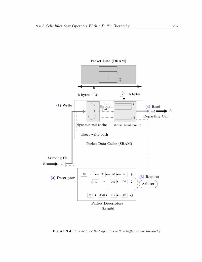
8.4 A Scheduler that Operates With a Buffer Hierarchy 237
1
Q
64... 9690
260101
40
70
1194001101
...40 Arbiter
R 40
Arriving Cell
(1) Write
Packet Descriptors
(4) ReadR64
Departing Cell
(3) Request(2) Descriptor
...
(Length)
Packet Data (DRAM)
1
Q
1
Q
b bytes
cut
paththrough
static head cachedynamic tail cache
direct-write path
Packet Data Cache (SRAM)
W R b bytes
Figure 8.4: A scheduler that operates with a buffer cache hierarchy.

8.5 A Scheduler Hierarchy that Operates With a Buffer Hierarchy 238
NObservation 8.4. Recall that the packet buffer cache allocates memory to the
queues in blocks of b-bytes each. Consecutive packets destined for a
queue are packed back to back, occupying consecutive locations in
memory.8 From the scheduler’s perspective, this means that it no
longer needs to store the address of every packet. The buffer cache
simply streams out the required number of bytes from the location
where the last packet for that queue was read.
Based on the observation above, the scheduler can eliminate storing per-packet
addresses, and only needs to store packet addresses and a pointer to the next descriptor.
This would reduce the size of the packet descriptor to 6 bytes.
Example 8.6. For example, on a 100 Gb/s link with a 10 ms packet buffer, a
scheduler database that stores a 6-byte descriptor for each smallest-size
40-byte packet would need approximately 150 Mb of SRAM. This is
smaller in size than the scheduler implementation shown in Example 8.4.
8.5 A Scheduler Hierarchy that Operates With a
Buer Hierarchy
Of course, we can now build a cache-based implementation for our scheduler, identical
to the approach we took in Section 8.3. As a consequence, the implementation of the
scheduler that operates with the buffer cache is the same as shown in Figure 8.4. The
only difference is that the implementation of the scheduler is itself cached as shown in
Figure 8.5. We can derive the following results:
8Note that the buffer cache manages how these b-byte blocks are allocated and linked. Thebuffer cache does not need to maintain per-packet descriptors to store these packets; it only needsto maintain and link b-byte blocks. If these b-byte blocks are themselves allocated for a queuecontiguously in large blocks of memory, i.e., “pages”, then only these pages need to be linked. Sincethe number of pages is much smaller than the total number of cells or minimum-size packets, this iseasy for the buffer cache to manage.

8.5 A Scheduler Hierarchy that Operates With a Buffer Hierarchy 239
Arbiter
R 40
Arriving Cell
(1) Write (4) ReadR64
Departing Cell
(3) Request(2) Descriptor
1
Q
cut
paththrough
static head cachedynamic tail cache
direct-write path
Packet Descriptor Cache (SRAM)(Length)
cut
paththrough
static head cachedynamic tail cache
direct-write path
1
Q2
6496
60101
40119
1
Q
...
2
9091
260101
... 40119
90
140
50
...
...
...
...
Packet Descriptors (DRAM)
Packet Data Cache (SRAM)
Packet Data (DRAM)
1
Q
b bytes W R b bytes
Figure 8.5: A scheduler cache hierarchy that operates with a buffer cache hierarchy.

8.6 A Scheduler that Piggybacks on the Buffer Hierarchy 240
Corollary 8.2. (Sufficiency) A scheduler (which only stores packet lengths) requires
no more than Qb(4 + lnQ) log2 PmaxPmin
bytes in its cache, where Pmin, Pmax are the
minimum and maximum packet sizes supported by the scheduler.
Proof. This is a direct consequence of adding up the cache sizes derived from Theo-
rems 7.1 and 7.3. From Theorem 7.1, we know that the tail cache must be at least Qb
bytes if packet data is being stored in a buffer. However, the scheduler only needs
to store a descriptor of size log2 Pmax bytes (to encode the packet length) for every
Pmin bytes stored by the corresponding packet buffer. So, the size of the cache is
reduced by a factor of log2 PmaxPmin
bytes. This implies that the size of the tail cache is no
more than Qb log2 PmaxPmin
bytes. Similarly, the size of the head cache can be inferred from
Theorem 7.3 to be Qb(3 + lnQ) log2 PmaxPmin
bytes. Summing the sizes of the two caches
gives us the result. r
Example 8.7. For example, on a 100 Gb/s link with a 10 ms packet buffer, the
scheduler database can be stored using an on-chip cache and an off-chip
external DRAM. Our results indicate that with a DRAM with a capacity
of 50 Mb and TRC = 51.2ns; b = 640 bytes, and Q = 96 scheduler
queues, the scheduler cache size would be less than 250 Kb, which can
easily fit in on-chip SRAM. Both the capacity of the external memory
and the cache size are smaller in this implementation, compared to the
results shown in Example 8.5.
8.6 A Scheduler that Piggybacks on the Buer Hi-
erarchy
In the previous section, we eliminated the need for maintaining per-packet addresses
in the scheduler. This was possible because consecutive packets were packed back
to back in consecutive addresses, and these addresses were maintained by the buffer
cache hierarchy. However, the method described above requires the scheduler to keep
a linked list of packet lengths. In this section we show how the scheduler can eliminate

8.6 A Scheduler that Piggybacks on the Buffer Hierarchy 241
the need for maintaining packet lengths, and so eliminate maintaining descriptors
altogether!
In the technique that we describe, our scheduler will piggyback on the packet buffer
cache hierarchy. Observe that packets already carry the length information that a
scheduler maintains.9 This motivates the following idea:
DIdea. “The buffer cache could retrieve the lengths of the packets, which are
pre-fetched in the head cache, and pass on these lengths to the scheduler a priori,
just in time for the arbiter to make decisions on which packets to schedule.a”
aThe crux of the method can be captured in the mythical conversation between thescheduler and buffer (involving the arbiter) in Box 8.1.
8.6.1 Architecture of a Piggybacked Scheduler
Figure 8.6 describes the architecture of a piggybacked scheduler. The following
describes how the scheduler and the buffer interact.
1. Arriving packets are written to the tail of the packet buffer cache.
2. Descriptors for the packet are not created. Note that this implies that the
scheduler does not need to be involved when a packet arrives.
3. The length of the packet is encoded along with the packet data. In most cases
this is not necessary, since packet length information is already part of the packet
header — if not, then the length information is tagged along with the packet.
In what follows, we assume that the packet length is available at (or tagged in
front of) the most significant byte of the packet header.10
9The length of a packet is usually part of a protocol header that is carried along with the packetpayload. In case of protocols where the length of a packet is not available, the packet length can beencoded by, for example, preceding the packet data with length information at the time of buffering.
10Note that the packet length field can always be temporarily moved to the very front of thepacket when it is buffered. The length field can be moved back to its correct location after it is readfrom the buffer, depending on the protocol to which the packet belongs.

8.6 A Scheduler that Piggybacks on the Buffer Hierarchy 242
1
Q
Write
cut-through
static head cachedynamic tail cache
direct-write path
length parser
Length
1
Q
Descriptor Cache
Request
Arbiter
Read
(1, 3)
(5)
(6)
(7)
(Packet Lengths)
R40
Departing Cell
R 40
Arriving Cell
Fetch(4)
Descriptor
(2)
Packets and Encoded Lengths (Cache)
Packet and Encoded Lengths (DRAM)
1
Q
b bytes W R b bytes
& Parse L1
L2 + L3
L4
L4 is the latency for length parsing and the length interfaceL1 + L2 + L3 + L4 is the total latency between the buffer and scheduler/arbiter
L1 is the latency on the request interfaceL2 + L3 is the total round-trip memory latency
Figure 8.6: A combined packet buffer and scheduler architecture.

8.6 A Scheduler that Piggybacks on the Buffer Hierarchy 243
4. The buffer memory management algorithm periodically fetches b-bytes blocks of
data for a queue and replenishes the cache. When the packets are fetched into
the head cache, their lengths are parsed and sent to the scheduler. The queue to
which the corresponding packet belongs is also conveyed to the scheduler.
5. The scheduler caches the length information for these packets, and arranges
them based on the queues that the packets are destined to.
6. Based on the network policy, the arbiter chooses a queue to service, dequeues a
descriptor, and issues a read for a packet from the buffer.
7. On receiving this request, the buffer cache streams the packet from its head
cache.
Note that there is no need to maintain a separate descriptor linked list for the
scheduler. The linked list information is created on the fly! — and is made available
just in time so that an arbiter can read packets in any order that it chooses.
8.6.2 Interaction between the Packet Buer and Scheduler
Cache
We are not quite done. We need to ensure that the arbiter is work-conserving — i.e.,
if there is a packet at the head of any queue in the system, the descriptor (or packet
length in this case) for that packet is available for the arbiter to read, so that it can
maintain line rate. However, the system architecture shown in Figure 8.6 is an example
of a closed-loop system where the buffer cache, scheduler, and arbiter are dependent
on each other. We need to ensure that there are no deadlocks, loss of throughput, or
starvation.
Let us consider the series of steps involved in ensuring that the packet scheduler
always has enough descriptors for the arbiter to schedule at line rate. First note that,
by design, the arbiter will always have the length descriptors (delayed by at most
L4 time slots) for any data already residing in the head cache. Our bigger concern
is: How can we ensure that the arbiter does not have to wait to issue a read for a
packet that is waiting to be transferred to the head cache? We consider the system
8.6 A Scheduler that Piggybacks on the Buffer Hierarchy 244
Box 8.1: A Buer and Scheduler Converse
The scheduler and buffer (played by Fraulein S. Duler and B. Uffer) are discussinghow to maintain packet lengths as needed by the Arbiter (played by Herr Biter).a
B. Uffer: Why do you maintain lengths of all packets in your linked lists?
S. Duler: So that I can know the exact size of the packets from each of your queues. HerrBiter is very particular about packet sizes.
B. Uffer: Why does he need the exact size? He could read one MTU’s (maximumtransmission unit) worth from the head of each queue. He could parse the lengthsby reading the packet headers, and send the exact number of bytes down the wire.
S. Duler: But the packet could be less than one MTU long.
B. Uffer: In that case, he could buffer the residual data.
S. Duler: Oh — I am not so sure he can do that : : :
B. Uffer: Why? Surely, Herr Biter can read?
S. Duler: Of course! The problem is that he would need to store almost one MTU foreach queue in the worst case.
B. Uffer: What’s the big deal?
S. Duler: He doesn’t have that much space!
B. Uffer: That’s his problem!
S. Duler: Oh, come on. We all reside on the same ASIC.
B. Uffer: Well, can’t he buffer the residual data for every queue?
S. Duler: Look who’s talking!; I thought it was your job to buffer packets!
B. Uffer: I was trying to save you from keeping the lengths of all packets : : :
S. Duler: Then come up with something better : : :
B. Uffer: Wait, I have an idea! I can send you the length of the head-of-line packet fromevery queue.
S. Duler: How will you do that?
B. Uffer: Well, I have pre-fetched bytes from every queue in my head cache. When datais pre-fetched, I can parse the length, and send it to you before Herr Biter needs it.
S. Duler: Yes — then I won’t need to keep a linked list of lengths for all packets!
B. Uffer: But what about Herr Biter? Would he have the packet length on time, whenhe arbitrates for a packet?
S. Duler: Trust me, he’s such a dolly! He will never know the difference! : : :
aFraulein (Young lady), Herr (Mister) in German.

8.6 A Scheduler that Piggybacks on the Buffer Hierarchy 245
Arbiter dequeues descriptor and
Packet is read from head cachecreating deficit for queue N
Parser retrieves and sends length of
Queue N is selected for replinishment
requests packet for queue N
to head cache
L1 L3
L2
L4
ReplinishRead
Request Retrieve
L2 + L3 is the total round-trip memory latencyL1 + L2 + L3 + L4 is the total latency between the buffer and scheduler/arbiter
new packet to scheduler for queue N
Figure 8.7: The closed-loop feedback between the buffer and scheduler.
from an arbiter’s perspective and focus on a particular queue, say queue N , as shown
in Figure 8.7.
1. Request: The arbiter dequeues a descriptor for queue N and requests a packet
from queue N .
2. Read: The buffer cache receives this read request after a fixed time L1 (this
corresponds to the delay in step 6 in Figure 8.6), and streams the requested
packet on the read interface.
3. Replenish: This creates a deficit for queue N in the head cache. If at this time
queue N had no more data in the head cache,11 then the descriptors for the next
packet of queue N will not be available. However, we are assured that at this
time queue N will be the most-deficited queue or earliest critical queue (based
on the algorithms described in Chapter 7). The buffer cache sends a request to
11If queue N had additional data in the head cache, then by definition the scheduler has thelength information for the additional data in head cache.

8.6 A Scheduler that Piggybacks on the Buffer Hierarchy 246
replenish queue N . We will denote L2 to be the time that it takes the buffer
cache to react and send a request to replenish queue N . This corresponds to
part of the latency in step 4 in Figure 8.6.
4. Retrieve: The packet data for queue N is received from either the tail cache
or the external memory after L312 time slots. The length of the next packet
for queue N is retrieved and sent to the scheduler. This corresponds to the
other part of the latency in step 4 in Figure 8.6. Note that L2 and L3 together
constitute the round-trip latency of fetching data from memory.
5. Request: The scheduler receives the new length descriptor for queue N after
L4 time slots. This is the latency incurred in transferring data on the length
interface in step 5 in Figure 8.6.
So, if the arbiter has no other descriptor available for queue N , then it will have
to wait until the next descriptor comes back, after L = L1 + L2 + L3 + L4 time slots,
before it can make a new request and fetch more packets for queue N from the buffer.
This can result in loss of throughput, as shown in the following counter-example:
Example 8.8. The adversary runs the worst-case adversarial traffic pattern as
described in Theorem 7.2, from time slot T = 0 to T = E, where E is
the total time it takes to run the worst-case adversarial pattern. This
pattern results in creating the maximum deficit for a particular queue
(in this case, queue N). Since queue N is the most-deficited queue,
the buffer will issue a request to replenish the head cache for that
queue. However, the adversary could simultaneously request data from
queue N at line rate. Notice that it would take another L time slots
for the length of the next packet to be retrieved and made available
to the scheduler. Thus the arbiter cannot request any packets from
queue N between time E and time E + L. This pattern can be
12L3 denotes the worst-case latency to fetch data from either external memory or tail cache.However, in practice it is always the latency to fetch data from external memory, because it usuallytakes much longer to fetch data from external memory than from on-chip tail cache.

8.6 A Scheduler that Piggybacks on the Buffer Hierarchy 247
t
E0 ......
Adversarial
E + L
1 2
Lost Next Packets
(a) Head cache empty
Q1
Q2
Q3
Q4
Q5
Q6
Q7
QN-1
QN
QN-2
Descriptor Cache
Arbiter
(Packet Lengths)1
Q
W R
Q1
Q2
Q3
Q4
Q5
Q6
Q7
QN-1
QN
QN-2
(c) Cache replinish issued(b) Scheduler cache empty
For Queue N (Time E): (a) Arbiter dequeues length (b) Arbiter issues packet read
For Queue N (Time E+L):
(a) No packets read by arbiterFor Queue N (E < Time < E+L):
Packets and Encoded Lengths (Head Cache)
Packets and Encoded Lengths(DRAM)
Pattern Throughput Streamed
(b) No packets streamed by buffer (c) Cache replinish data received by buffer (d) Next packet length parsed and sent to scheduler
From Tail Cache
... Packets ... Packets ...
Packets Lengths ...
Figure 8.8: The worst-case pattern for a piggybacked packet scheduler.
repeated continuously over time over different queues, causing a loss
of throughput as shown in Figure 8.8.

8.6 A Scheduler that Piggybacks on the Buffer Hierarchy 248
Box 8.2: Applications that Need Scheduling
In the last decade, a near-continuous series of new Internet-based applications (“killerapps”) have entered widespread use. Each new application has introduced support challengesfor its implementation over the current “best-effort” network infrastructures, and forrestricting the amount of network resources that it consumes.
In the earliest days of the Internet, the most common application, email, requiredonly best-effort service, but by 1995 the advent of the browser introduced widespreadadoption of Web protocols. The Internet was now used primarily for content sharing anddistribution and required semi-real-time support. At the same time, applications for remotecomputer sharing became common, including telnet, ssh, and remote login. Although theseapplications didn’t require high bandwidth, they ideally called for low latency.
By the late 1990s, the Internet had begun to be used to support E-commerce appli-cations, and new routers were designed to identify these applications and provide broadquality-of-service guarantees. Load balancers and other specialized router equipment werebuilt to provide optimally reliable service with zero packet drop for these financially sensitiveapplications.
In 1999, the first large-scale P2P protocol, freenet [188] was released. Freenet initiateda wave of popular file sharing tools, such as Napster, Kazaa, etc., to transfer large files,including digital content. P2P protocols have continued to evolve over the last eight years,and now place heavy bandwidth demands on the network. It has been estimated that over70% of all Internet traffic consists of P2P traffic, and many businesses, universities, andInternet service providers (ISPs) now schedule, police, and limit this traffic.
By 2000, the Internet had begun to see widespread adoption of real-time communicationapplications such as Internet chat [189], instant messaging, etc. These applications wereextremely sensitive to latency and jitter — for example, conversation quality is known todegrade when latency of communication exceeds ∼150ms. Thus, it would be another 5-6years before business- and consumer-quality Internet telephony [190] became widespread.
The past few years have seen the advent of real-time, multi-point applications requiringassured bandwidth, delay, and jitter characteristics. These applications include multiplayergames [191],a videoconferencing applications such as Telepresence [28], and IPTV [29].
Additionally, storage protocols [61] mandate high-quality communications with nopacket drops, and inter-processor communications networks for supercomputing applicationsmandate extremely low latency. There is even an ongoing interest in using the Internetfor sensitive and mission-critical applications, e.g., distributed orchestras and tele-surgery.All of these applications require a scheduler to differentiate them and provide the requisitequality of service.
With the ever-increasing range of applications, and their ever-changing demands, theneed for scheduling has become correspondingly important. Thus, today nearly all switchesand routers, including home office and small office units, support scheduling.
aThe earliest example was Doom [192], released in 1993.

8.6 A Scheduler that Piggybacks on the Buffer Hierarchy 249
8.6.3 A Work-conserving Packet Scheduler
To ensure that the scheduler is work-conserving, we will need to size both the packet
buffer and the scheduler cache carefully. We are now ready to derive their sizes.
Theorem 8.1. (Sufficiency) The MDQF packet buffer requires no more than
Q [b(4 + lnQ) +RL] bytes in its cache in order for the scheduler to piggyback on
it, where L is the total closed-loop latency between the scheduler and the MDQF buffer
cache.
Proof. We know that if the buffer does not have a scheduler that piggybacks on it,
then the size of the head cache is Q[b(3 + lnQ)] (from Theorem 7.3), and the size of
the tail cache is Qb bytes (from Theorem 7.1). In order to prevent the adversarial
traffic pattern described in Example 8.8, we will increase the size of the head cache
by RL bytes for every queue. This additional cache completely hides the round-trip
latency L between the buffer and the scheduler. Summing up the above numbers, we
have our result. r
Theorem 8.2. (Sufficiency) A length-based packet scheduler that piggybacks on the
MDQF packet buffer cache requires no more than Q [b(3 + lnQ) +RL] log2 PmaxPmin
bytes
in its head cache, where L is the total closed-loop latency between the scheduler and
the MDQF buffer cache.
Proof. This is a consequence of Theorem 8.1 and Corollary 8.2. Note that the scheduler
cache only needs to keep the lengths of all packets that are in the head cache of the
packet buffer. From Theorem 8.1, the size of the head cache of the packet buffer is
Q[b(3 + lnQ)] bytes. Corollary 8.2 tells us that we need to scale the size of a length-
based scheduler cache by log2 PmaxPmin
bytes. So the size of the cache for the scheduler is
Q[b(3 + lnQ)] log2 PmaxPmin
bytes. Note that the scheduler does not need a tail cache, hence
its scaled size does not include the Qb log2 PmaxPmin
bytes that would be required if it had a
tail cache. r

8.7 Design Options and Considerations 250
Table 8.1: Packet buffer and scheduler implementation options.
Buf-fer14
Sche-duler
Desc-riptor
Pros ConsSec-tion
U ULength,Address,NextPtr
SimpleHard to scale buffer,
scheduler performance8.2
U CLength,Address
Reduces scheduler size, scalesscheduler performance
Hard to scale bufferperformance
8.3
C ULength,NextPtr
Reduces scheduler size, scalesbuffer performance
Hard to scale schedulerperformance
8.4
C C LengthMinimizes scheduler size,
scales buffer and schedulerperformance
Requires two caches 8.5
Piggybacked NoneEliminates need for scheduler
memory, scales buffer andscheduler performance
Sensitive to latency L,requires modification to
caching hierarchy8.6
Example 8.9. For example, on a 100 Gb/s link with a 10 ms packet buffer, the
scheduler database can be stored using an on-chip cache. It does not
require an off-chip external DRAM, since the lengths are piggybacked
on the packets in the packet buffer. Our results indicate that with a
DRAM with TRC = 51.2 ns used for the packet buffer, b = 640 bytes,
and Q = 96 scheduler queues, and latency L = 100 ns, the buffer cache
size would be less than 5.4 Mb, and the scheduler cache size would be
less than 270 Kb, which can easily fit in on-chip SRAM. The size of
the scheduler database is almost identical13 to the results derived in
Example 8.7, except that no separate DRAM needs to be maintained
to implement the packet scheduler!
8.7 Design Options and Considerations
We have described various techniques to scale the performance of a packet scheduler.
Table 8.1 summarizes the pros and cons of the different approaches. Note that we do
not mandate any one technique over the other, and that each technique has its own
tradeoffs, as discussed below.
13This can change if the latency L becomes very large.14Note that U in Table 8.1 and Table 8.2 refers to an un-cached implementation, and C refers to
an implementation that uses a caching hierarchy.

8.7 Design Options and Considerations 251
1. If the total size of the scheduler and buffer is small, or if the line rates supported
are not very high, the scheduler can be implemented in a typical manner as
suggested in Section 8.2. It may be small enough that both the scheduler and
buffer can fit on-chip — this is typically the case for the low-end Ethernet switch
and router markets.
2. The solution in Section 8.3 is used when the buffer cache cannot fit on-chip, but
a scheduler cache (which is typically smaller than the buffer cache) can. This
can happen when the number of queues is very large, or the available memory
is very slow compared to the line rate, both of which mandate a large buffer
cache size. We have targeted the above implementation for campus backbone
routers [109] where the above requirements hold true.
3. The solution in Section 8.4 is used when the number of packets that are to
be supported by a scheduler is not very large, even though the buffer itself is
large. This happens in applications that pack multiple packets into super frames.
Since the scheduler only needs to track a smaller number of super frames, the
size of the scheduler database is small and no caching hierarchy is needed for
the scheduler. We have targeted the above implementations for schedulers that
manage VOQs in the Ethernet switch and Enterprise router markets [193].
4. The solution in Section 8.5 allows scaling the performance of both the buffer
and the scheduler to very high line rates, since both the buffer and scheduler
are cached; however, it comes at the cost of implementing two separate caching
hierarchies. We currently do not implement this technique, because the method
described below is a better tradeoff for current-generation 10− 100 Gb/s line
cards. However, we believe that if the memory latency L becomes large, this
technique will find favor compared to the technique below, where cache size
depends on the memory latency.
5. Finally, the solution in Section 8.6 is the most space-efficient, and completely
eliminates the need for a scheduler database. However, it requires a modified
caching hierarchy where the buffer and scheduler interact closely with each
other. Also, if the round trip latency L is large (perhaps due to a large external
memory latency), the cache size required may be larger than the sum of the

8.8 Conclusion 252
Table 8.2: Packet buffer and scheduler implementation sizes.
BufferSche-duler
Buffer CacheSize
Scheduler Cache SizeBufferMainMem.
Sche-dulerMainMem.
Section
U U - - SRAM SRAM 8.2
U C - Qb(4 + lnQ)|D|Pmin
SRAM DRAM 8.3
C U Qb(4 + lnQ) - DRAM SRAM 8.4
C C Qb(4 + lnQ) Qb(4 + lnQ)log2 Pmax
PminDRAM DRAM 8.5
Piggy Backed Q [b(4 + lnQ) +RL] Q [b(3 + lnQ) +RL]log2 Pmax
PminDRAM - 8.6
cache sizes if both the buffer cache and the scheduler cache are implemented
separately (as suggested in Section 8.5). This technique is by far the most
common implementation, and we have used it widely, across multiple instances
of data-path ASICs for 10− 100 Gb/s line cards in the high-speed Enterprise
market.
NObservation 8.5. Some schedulers keep additional information about a packet in
their descriptors. For example, some Enterprise routers keep packet
timestamps, so that they can drop packets that have spent a long time
in the buffer (perhaps due to network congestion). The techniques
that we describe here are not limited to storing only addresses and
packet lengths; they can also be used to store any additional descriptor
information.
Table 8.2 summarizes the sizes of the buffer and scheduler for the various implemen-
tation options described in this chapter. Table 8.3 provides example implementations
for the various techniques for a 100Gb/s line card. All the examples described in
Table 8.3 are for Q = 96 queues and an external DRAM with a TRC of 51.2 ns and a
latency of L = 100 ns.
8.8 Conclusion
High-speed routers need packet schedulers to maintain descriptors to every packet
in the buffer, so that the router can arbitrate among these packets and control their
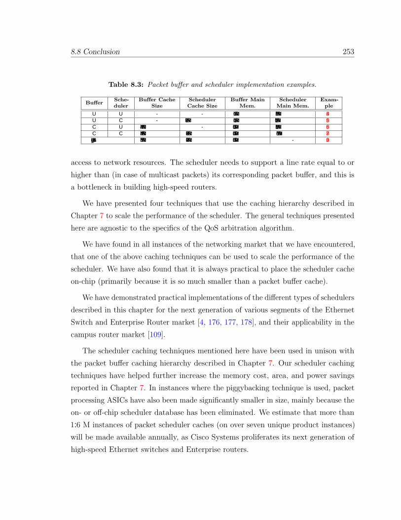
8.8 Conclusion 253
Table 8.3: Packet buffer and scheduler implementation examples.
BufferSche-duler
Buffer CacheSize
SchedulerCache Size
Buffer MainMem.
SchedulerMain Mem.
Exam-ple
U U - - 1Gb SRAM 250Mb SRAM 8.4
U C - 700Kb SRAM 1Gb SRAM 150Mb DRAM 8.5
C U 4.4Mb SRAM - 1Gb DRAM 150Mb SRAM 8.6C C 4.4Mb SRAM 250kb SRAM 1Gb DRAM 50Mb DRAM 8.7
Piggy Backed 5.3Mb SRAM 270kb SRAM 1Gb DRAM - 8.9
access to network resources. The scheduler needs to support a line rate equal to or
higher than (in case of multicast packets) its corresponding packet buffer, and this is
a bottleneck in building high-speed routers.
We have presented four techniques that use the caching hierarchy described in
Chapter 7 to scale the performance of the scheduler. The general techniques presented
here are agnostic to the specifics of the QoS arbitration algorithm.
We have found in all instances of the networking market that we have encountered,
that one of the above caching techniques can be used to scale the performance of the
scheduler. We have also found that it is always practical to place the scheduler cache
on-chip (primarily because it is so much smaller than a packet buffer cache).
We have demonstrated practical implementations of the different types of schedulers
described in this chapter for the next generation of various segments of the Ethernet
Switch and Enterprise Router market [4, 176, 177, 178], and their applicability in the
campus router market [109].
The scheduler caching techniques mentioned here have been used in unison with
the packet buffer caching hierarchy described in Chapter 7. Our scheduler caching
techniques have helped further increase the memory cost, area, and power savings
reported in Chapter 7. In instances where the piggybacking technique is used, packet
processing ASICs have also been made significantly smaller in size, mainly because the
on- or off-chip scheduler database has been eliminated. We estimate that more than
1.6 M instances of packet scheduler caches (on over seven unique product instances)
will be made available annually, as Cisco Systems proliferates its next generation of
high-speed Ethernet switches and Enterprise routers.

8.8 Conclusion 254
In summary, the techniques we have described can be used to build schedulers that
are (1) extremely cost-efficient, (2) robust against adversaries, (3) give the performance
of SRAM with the capacity characteristics of a DRAM, (4) are faster than any that
are commercially available today, and (5) can be scaled for several generations of
technology.
Summary
1. The current Internet is a packet switched network. This means that hosts can join and
leave the network without explicit permission. Packets between communicating hosts are
statistically multiplexed across the network and share network and router resources (e.g.,
links, routers, buffers, etc.).
2. In order for the Internet to support a wide variety of applications (each of which places
different demands on bandwidth, delay, jitter, latency, etc.), routers must first differentiate
these packets and buffer them in separate queues during times of congestion. Then an
arbiter provides these packets their required quality of service and access to network
resources.
3. Packet schedulers facilitate the arbiter’s task by maintaining information (“descriptors”)
about every packet that enters a router. These descriptors are linked together to form
descriptor linked lists, and are maintained for each queue in the buffer. The descriptor
linked lists are also responsible for specifying the order of packets in a queue.
4. A typical descriptor in the packet scheduler contains the packet length, an address to the
location of the packet in the buffer, and a pointer to the next descriptor that corresponds
to the next packet in the queue.
5. A packet buffer, a scheduler, and an arbiter always operate in unison, so a scheduler needs
to operate at least as fast as a packet buffer, and in some cases faster, due to the presence
of multicast packets.
6. Maintaining scheduling information was easy at low speeds. However, above 10 Gb/s
(similar to packet buffering), descriptors begin arriving and departing faster than the
access time of a DRAM, so packet scheduling is now a significant bottleneck in scaling
the performance of a high-speed router.
7. Similar to packet buffering (see Chapter 7), a caching hierarchy is an appealing way to
build packet schedulers. We present four different techniques to build schedulers (in unison


8.8 Conclusion 256
compromised either now or, provably, ever in future.
17. These techniques are practical and have been implemented in fast silicon in multiple
high-speed Ethernet switches and Enterprise routers.

Chapter 9: Designing Statistics Counters from
Slower MemoriesApr 2008, Sonoma, CA
Contents
9.1 Introduction . . . . . . . . . . . . . . . . . . . . . . . . . . . . . . . . 259
9.1.1 Characteristics of Measurement Applications . . . . . . . . . . . . . . 261
9.1.2 Problem Statement . . . . . . . . . . . . . . . . . . . . . . . . . . . . . 263
9.1.3 Approach . . . . . . . . . . . . . . . . . . . . . . . . . . . . . . . . . . 263
9.2 Caching Memory Hierarchy . . . . . . . . . . . . . . . . . . . . . . . 265
9.3 Necessity Conditions on any CMA . . . . . . . . . . . . . . . . . . . 267
9.4 A CMA that Minimizes SRAM Size . . . . . . . . . . . . . . . . . . 268
9.4.1 LCF-CMA . . . . . . . . . . . . . . . . . . . . . . . . . . . . . . . . . 268
9.4.2 Optimality . . . . . . . . . . . . . . . . . . . . . . . . . . . . . . . . . 269
9.4.3 Sufficiency Conditions on LCF-CMA Service Policy . . . . . . . . . . 270
9.5 Practical Considerations . . . . . . . . . . . . . . . . . . . . . . . . . 273
9.5.1 An Example of a Counter Design for a 100 Gb/s Line Card . . . . . . 273
9.6 Subsequent Work . . . . . . . . . . . . . . . . . . . . . . . . . . . . . 275
9.7 Conclusions . . . . . . . . . . . . . . . . . . . . . . . . . . . . . . . . . 275
List of Dependencies
• Background: The memory access time problem for routers is described in
Chapter 1. Section 1.5.3 describes the use of caching techniques to alleviate
memory access time problems for routers in general.
Additional Readings
• Related Chapters: The caching hierarchy described in this chapter was first
described to implement high-speed packet buffers in Chapter 7. A similar
technique is also used in Chapter 8 to implement high-speed packet schedulers.

Table: List of Symbols.
T Time SlotTRC Random Cycle Time of MemoryM Total Counter Widthm Counter Width in CacheP Minimum Packet SizeR Line RateN Number of Counters
C(i; t) Value of Counter i at Time t
b Number of Time Slots between Updates to DRAM
Table: List of Abbreviations.
LCF Longest Counter FirstCMA Counter Management Algorithm
SRAM Static Random Access MemoryDRAM Dynamic Random Access Memory

“There are three types of lies - lies, damn lies, and
statistics”.
— Benjamin Disraeli† 9Designing Statistics Counters from Slower
Memories
9.1 Introduction
Many applications on routers maintain statistics. These include firewalling [194]
(especially stateful firewalling), intrusion detection, performance monitoring (e.g.,
RMON [195]), network tracing, Netflow [196, 197, 198], server load balancing, and
traffic engineering [199] (e.g., policing and shaping). In addition, most routers maintain
statistics to facilitate network management.
Example 9.1. Figure 9.1 shows four examples of measurement counters in a network
— (a) a storage gateway keeps counters to measure disk usage statistics,
(b) the central campus router maintains measurements of users who
attempt to maliciously set up connections or access forbidden data, (c)
a local bridge keeps usage statistics and performs load balancing and
directs connections to the least-loaded web-server, and (d) a gateway
router that provides connectivity to the Internet measures customer
traffic usage for billing purposes.
†Also variously attributed to Alfred Marshall and Mark Twain.
259

9.1 Introduction 260
(d) Bandwidth
Campus
(2) Malicious ISP
Gateway
( 3 ) H o s t A c c e s s i n g(4) Host Accessing Server FarmLocal BridgeStorage Network
Network
Figure 9.1: Measurement infrastructure.

9.1 Introduction 261
The general problem of statistics maintenance can be characterized as follows:
When a packet arrives, it is first classified to determine which actions will be performed
on the packet — for example, whether the packet should be accepted or dropped,
whether it should receive expedited service or not, which port it should be forwarded
to, and so on. Depending on the chosen action, some statistics counters are updated.
We are not concerned with how the action to be performed is identified. The
task of identification of these actions is usually algorithmic in nature. Depending on
the application, many different techniques have been proposed to solve this problem
(e.g., address lookup [134], packet classification [184], packet buffering [173, 174], QoS
scheduling [186], etc.).
We are concerned with the statistics that these applications measure, once the
action is performed and the counter to be updated (corresponding to that action) is
identified. The statistics we are interested in here are those that count events: for
example, the number of fragmented packets, the number of dropped packets, the
total number of packets arrived, the total number of bytes forwarded to a specific
destination, etc. In the rest of this chapter we will refer to these as counters.
As we will see, almost all Ethernet switches and Internet routers maintain statistics
counters. At high speeds, the rate at which these counters are updated causes a
memory bottleneck. It is our goal to study and quantitatively analyze the problem of
maintaining these counters,1 and we are motivated by the following question — How
can we build high-speed measurement counters for routers and switches, particularly
when statistics need to be updated faster than the rate at which memory can be accessed?
9.1.1 Characteristics of Measurement Applications
Note that if we only want to keep measurements for a particular application, we could
exploit the characteristics of that application to build a tailored solution. For example,
in [201], Estan and Varghese exploit the heavy-tailed nature of traffic to quickly
1Our results were first published in [200], and we were not aware of any previous work thatdescribes the problem of maintaining a large number of statistics counters.

9.1 Introduction 262
identify the largest flows and count them (instead of counting all packets and flows
that arrive) for the Netflow application [196, 197].
NObservation 9.1. Most high-speed routers offer limited capability to count packets
at extremely high speeds. Cisco Systems’ Netflow [196] can sample
flows, but the sampling only captures a fraction of the traffic arriving
at line rate. Similarly, Juniper Networks [197] can filter a limited set of
flows and maintain statistics on them.
But we would like a general solution that caters to a broad class of applications
that have the following characteristics:
1. Our applications maintain a large number of counters. For example, a routing
table that keeps a count of how many times each prefix is used, or a router that
keeps a count of packets belonging to each TCP connection. Both examples
would require several hundreds of thousands or even millions of counters to be
maintained simultaneously, making it infeasible (or at least very costly) to store
them in SRAM. Instead, it becomes necessary to store the counters in off-chip,
relatively slow DRAM.
2. Our applications update their counters frequently. For example, a 100 Gb/s
link in which multiple counters are updated upon each packet arrival. These
read-modify-write operations must be conducted at the same rate as packets
arrive.
3. Our applications mandate that the counter(s) be correctly updated every time a
packet arrives; no packet must be left unaccounted for in our applications.
4. Our applications require measurement at line rates without making any assump-
tions about the characteristics of the traffic that contribute to the statistics.
Indeed, similar to the assumptions made in Chapter 7, we will require hard perfor-
mance guarantees to ensure that we can maintain counters for these applications
at line rates, even in the presence of an adversary.

9.1 Introduction 263
The only assumption we make is that these applications do not need to read the
value of counters in every time slot.2 They are only interested in updating their
values. From the viewpoint of the application, the counter update operation can be
performed in the background. Over time, a control path processor reads the values of
these counters (typically once in a few minutes on most high-speed routers) for post
processing and statistics collection.
9.1.2 Problem Statement
If each counter is M bits wide, then a counter update operation is as follows: 1) read
the M bit value stored in the counter, 2) increment the M bit value, and 3) write the
updated M bit value back. If packets arrive at a rate R Gb/s, the minimum packet
size is P bits, and if we update C counters each time a packet arrives, the memory
may need to be accessed (read or written) every P/2CR nanoseconds.
Example 9.2. Let’s consider the example of 40- byte TCP packets arriving on
a 40 Gb/s link, each leading to the updating of two counters. The
memory needs to be accessed every 2 ns, about 25 times faster than
the random-access speed of commercial DRAMs today.
If we do an update operation every time a packet arrives, and update C counters
per packet, then the minimum bandwidth RD required on the memory interface
where the counters are stored would be at least 2RMC/P . Again, this can become
unmanageable as the size of the counters and the line rates increase.
9.1.3 Approach
In this chapter, we propose an approach similar to the caching hierarchy introduced
in Chapter 7, which uses DRAMs to maintain statistics counters and a small, fixed
amount of (possibly on-chip) SRAM. We assume that N counters of width M bits are
to be stored in the DRAM, and that N counters of width mM bits are stored in
2There are applications for which the value of the counter is required to make data-path decisions.We describe memory load balancing techniques to support these applications in Chapter 10.

9.1 Introduction 264
Arriving Packet
Large DRAM memory with N counters of width M bits
Read M bits Write M bits
Counter Management Algorithm
Small SRAM memory with N counters of width m < M bits
Large Counter
Small Counter
.. .. .. ..
..(Counter Update) (Low Order Bits)
(Full Counter)
Figure 9.2: Memory hierarchy for the statistics counters. A fixed-sized ingress SRAMstores the small counters, which are periodically transferred to the large counters in DRAM.The counters are updated only once every b time slots in DRAM.
SRAM. The counters in SRAM keep track of the number of updates not yet reflected
in the DRAM counters. Periodically, under the control of a counter management
algorithm (CMA), the DRAM counters are updated by adding to them the values in
the SRAM counters, as shown in Figure 9.2. The basic idea is as follows:
DIdea. “If we can aggregate and update the DRAM counters relatively
infrequently (while allowing for frequent on-chip SRAM updates), the memory
bandwidth requirements can be significantly reduced”.
We are interested in deriving strict bounds on the size of the SRAM such that –
irrespective of the arriving traffic pattern – none of the counters in the SRAM overflow,
or the access rate and bandwidth requirements on the DRAM are decreased, while
still ensuring correct operation of the counters.
We will see that the size of the SRAM, and the access rate of the DRAM, both
depend on the CMA used. The main result of this chapter is that there exists a CMA

9.2 Caching Memory Hierarchy 265
(which we call largest counter first, LCF) that minimizes the size of the SRAM. We
derive necessary and sufficient conditions on the sizes of the counters (and hence of
the SRAM that stores all these counters), and we prove that LCF is optimal. An
example of how this technique can be used is illustrated below.
Example 9.3. Consider a 100 Gb/s line card on a router that maintains a million
counters. Assume that the maximum size of a counter is 64 bits and
that each arriving packet updates one counter. Our results indicate
that a statistics counter can be built with a commodity DRAM [3] with
access time 51.2 ns, a DRAM memory bandwidth of 1.25 Gb/s, and
9 Mb of SRAM.
9.2 Caching Memory Hierarchy
We will now describe the memory hierarchy used to hold the statistics counters, and
in the sections that follow we will describe the LCF-CMA (Largest Counter First
Counter Management Algorithm).
ℵDenition 9.1. Minimum Packet Size, P : Packets arriving at a switch have
variable lengths. We will denote by P the minimum length that a
packet can have.
As mentioned in Chapter 1, we will choose to re-define the unit of time as necessary
to make our analysis simpler to understand. In what follows, we will denote a time
slot as the time taken to receive a minimum-sized packet at a link rate R. The SRAM
is organized as a statically allocated memory, consisting of separate storage space
for each of the N counters. We will assume from this point forward that an arriving
packet increments only one counter. If instead we wish to consider the case where C
counters are updated per packet, we can consider the line rate on the interface to be
CR.
Each counter is represented by a large counter of size M bits in the DRAM, and
a small counter of size m < M bits in SRAM. The small counter counts the most

9.2 Caching Memory Hierarchy 266
recent events, while the large counter counts events since the large counter was last
updated. At any time instant, the correct counter value is the sum of the small and
large counters.
Updating a DRAM counter requires a read-modify-write operation: 1) Read an M
bit value from the large counter, 2) Add the m bit value of the corresponding small
counter to the large counter, 3) Write the new M bit value of the large counter to
DRAM, and 4) Reset the small counter value.
In this chapter, we will assume that the DRAM access rate is slower than the
rate at which counters are updated in SRAM. And so, we will update the DRAM
only once every b time slots, where b > 1 is a variable whose value will be derived
later. So the I/O bandwidth required from the DRAM is RD = 2RM/Pb, and the
DRAM is accessed only once every At = Pb/2R time slots to perform a read or a
write operation. Thus, the CMA will update a large counter only once every b time
slots. We will determine the minimum size of the SRAM as a function g(.) and show
that it is dependent on N , M , and b. Thus, the system designer is given a choice of
trading off the SRAM size g(N,M, b) with the DRAM bandwidth RD and access time
At.3
ℵDenition 9.2. Count C(i, t): At time t, the number of times that the ith small
counter has been incremented since the ith large counter was last
updated.
ℵDenition 9.3. Empty Counter: A counter i is said to be empty at time t if
C(i, t) = 0.
We note that the correct value of a large counter may be lost if the small counter is
not added to the large counter in time, i.e., before an overflow of the small counter.
Our goal is to find the smallest-sized counters in the SRAM, and a suitable CMA,
3The variable b (b > 1) is chosen by the system designer. If b = 1, no SRAM is required, but theDRAM must be fast enough for all counters to be updated in DRAM.

9.3 Necessity Conditions on any CMA 267
such that a small counter cannot overflow before its corresponding large counter is
updated.4
9.3 Necessity Conditions on any CMA
Theorem 9.1. (Necessity) Under any CMA, a counter can reach a count C(i, t) of
ln[(b/(b− 1))(b−1)(N − 1)
]ln(b/(b− 1))
. (9.1)
Proof. We will argue that we can create an arrival pattern for which, after some time,
there exists k such that there will be (N − 1)/((b− 1)/b)k counters with count k + 1
irrespective of the CMA.
Consider the following arrival pattern. In time slot t = 1, 2, 3, . . . , N , small counter
t is incremented. Every bth time slot one of the large counters is updated, and
the corresponding small counter is reset to 0. So at the end of time slot N , there
are N(b − 1)/b counters with count 1, and N/b empty counters. During the next
N/b time slots, the N/b empty counters are incremented once more, and N/b2 of
these counters are now used to update the large counter and reset. So we now have
[N(b − 1)/b] + [N(b − 1)/b2] counters that have count 1. In a similar way, we can
continue this process to make N − 1 counters have a count of 1.
During the next time N − 1 slots, all N − 1 counters are incremented once, and
1/b of them are served and reset to zero. Now, assume that all of the remaining
approximately N/b empty counters are incremented twice in the next 2N/b time slots,5
while 2N/b2 counters become empty due to service. Note that the empty counters
decreased to 2N/b2 from N/b (if b = 2, there is no change). In this way, after some
time, we can have N − 1 counters of count 2.
4It is interesting to note that there is an analogy between the cache sizes for statistics countersand the buffer cache sizes that we introduced in Chapter 7. (See Box 9.1.)
5In reality, this is (N − 1)=b empty counters and 2(N − 1)=b time slots.

9.4 A CMA that Minimizes SRAM Size 268
By continuing this argument, we can arrange for all N − 1 counters to have a count
b− 1. Let us denote by T the time slot at which this first happens.
During the interval from time slot 2(N − 1) to 3(N − 1), all of the counters are
again incremented, and 1/b of them are served and reset to 0, while the rest have
a count of two. In the next N − 1 time slots, each of the counters with size 2 is
incremented and again 1/b are served and reset to 0, while the rest have a count of
three. Thus there are (N − 1)((b− 1)/b)2 counters with a count of three. In a similar
fashion, if only non-empty counters keep being incremented, after a while there will
be (N − 1)((b − 1)/b)k counters with count k + 1. Hence there will be one counter
with count:
ln(N − 1)
ln(b/(b− 1))=
ln(N − 1) + (b− 1) ln(b/(b− 1))
ln(b/(b− 1))
=ln[(b/(b− 1))(b−1)(N − 1)
]ln(b/(b− 1))
.
Thus, there exists an arrival pattern for which a counter can reach a count C(i, t)
ofln[(b/(b− 1))(b−1)(N − 1)
]ln(b/(b− 1))
. r
9.4 A CMA that Minimizes SRAM Size
9.4.1 LCF-CMA
We are now ready to describe a counter management algorithm (CMA) that will
minimize the counter cache size. We call this, longest counter first (LCF-CMA).

9.4 A CMA that Minimizes SRAM Size 269
Algorithm 9.1: The longest counter first counter management algorithm.
input : Counter Values in SRAM and DRAM.1
output: The counter to be replenished.2
/* Calculate counter to replenish */3
repeat every b time slots4
CurrentCounters ← SRAM [(1, 2, . . . , N)]5
/* Calculate longest counter */6
CMax ← FindLongestCounter(CurrentCounters)7
/* Break ties at random */8
if CMax > 0 then9
DRAM [CMax] = DRAM [CMax] + SRAM [CMax]10
/* Set replenished counter to zero */11
SRAM [CMax] = 012
/* Service update for a counter */13
repeat every time slot14
if ∃ update for c then15
SRAM [c] = SRAM [c] + UpdateCounter(c )16
Algorithm Description: Every b time slots, LCF-CMA selects the counter i
that has the largest count. If multiple counters have the same count, LCF-CMA picks
one arbitrarily. LCF-CMA updates the value of the corresponding counter i in the
DRAM and sets C(i, t) = 0 in the SRAM. This is described in Algorithm 9.1.
9.4.2 Optimality
Theorem 9.2. (Optimality of LCF-CMA) Under all arriving traffic patterns, LCF-
CMA is optimal, in the sense that it minimizes the count of the counter required.
Proof. We give a brief intuition of this proof here. Consider a traffic pattern from time
t, which causes some counter Ci (which is smaller than the longest counter at time t)
to reach a maximum threshold M∗. It is easy to see that a similar traffic pattern can

9.4 A CMA that Minimizes SRAM Size 270
cause the longest counter at this time t to exceed M∗. This implies that not serving
the longest counter is sub-optimal. A detailed proof appears in Appendix I. r
9.4.3 Suciency Conditions on LCF-CMA Service Policy
Theorem 9.3. (Sufficiency) Under the LCF-CMA policy, the count C(i, t) of every
counter is no more than
S ≡ ln bN
ln(b/(b− 1)). (9.2)
Proof. (By Induction) Let d = b/(b − 1). Let Ni(t) denote the number of counters
with count i at time t. We define the following Lyapunov function:
F (t) =∑i>1
diNi(t). (9.3)
We claim that under LCF policy, F (t) 6 bN for every time t. We shall prove this by
induction. At time t = 0, F (t) = 0 6 bN . Assume that at time t = bk for some k,
F (t) 6 bN . For the next b time slots, some b counters with count i1 > i2 > · · · > ib
are incremented. Even though not required for the proof, we assume that the counter
values are distinct for simplicity. After the counters are incremented, they have counts
i1 + 1, i2 + 1, . . . , ib + 1 respectively, and the largest counter among all the N counters
is serviced. The largest counter has at least a value C(.) > i1 + 1.
• Case 1 : If all the counter values at time t were nonzero, then the contribution
of these b counters in F (t) was: α = di1 + di2 + · · ·+ dib . After considering the
values of these counters after they are incremented, their contribution to F (t+ b)
becomes dα. But a counter with a count C(.) > i1 + 1 is served at time t+ b and
its count becomes zero. Hence, the decrease to F (t+ b) is at least dα/b. This is
because the largest counter among the b counters is served, and the contribution
of the largest of the b counters to the Lyapunov function must be at least greater

9.4 A CMA that Minimizes SRAM Size 271
than the average value of the contribution, dα/b. Thus, the net increase is at
most dα[1− (1/b)]− α. But d[1− (1/b)] = 1. Hence, the net increase is at most
zero; i.e., if arrivals occur to non-zero queues, F (t) can not increase.
• Case 2 : Now we deal with the case when one or more counters at time t were
zero. For simplicity, assume all b counters that are incremented are initially
empty. For these empty counters, their contribution to F (t) was zero, and their
contribution to F (t+ b) is db. Again, the counter with the largest count among
all N counters is served at time t + b. If F (t) 6 bN − db, then the inductive
claim holds trivially. If not, that is, F (t) > bN − db, then at least one of the
N − b counters that did not get incremented has count i∗ + 1, such that, di∗
> b;
otherwise, it contradicts the assumption F (t) > bN − db. Hence, a counter with
count at least i∗ + 1 is served, which decreases F (t + b) by di∗+1 = db. Hence
the net increase is zero. One can similarly argue the case when arrivals occur to
fewer than b empty counters.
Thus we have shown that, for all time t when the counters are served, F (t) 6 bN .
This means that the counter value cannot be larger than im, where, dim = Nb, i.e.,
C(.) 6ln bN
ln d. (9.4)
Substituting for d, we get that the counter value is bounded by S. r
Theorem 9.4. (Sufficiency) Under the LCF policy, the number of bits that are
sufficient per counter to ensure that no counter overflows, is given by
log2
ln bN
ln d. (9.5)
Proof. We know that in order to store a value x we need at most log2 x bits. Hence
the proof follows from Theorem 9.3.6 r
6It is interesting to note that the cache size is independent of the width of the counters beingmaintained.

9.4 A CMA that Minimizes SRAM Size 272
Box 9.1: Comparing Buers and Counters
9
1001
Unary :
Cluster 5 :
Decimal :
Binary :
IXRoman :
0100000000One-hot :
10111111111One-cold :
100Ternary :
Figure 9.3: Nu-meric Notations
A number can be represented in many notations, e.g., the number
9 is shown in five different notations in Figure 9.3. Most computing
systems (servers, routers, etc.) store numbers in binary or hexadecimal
format. In contrast, humans represent and manipulate numbers in
decimal (base-10) format. Each notation has its advantages and is
generally used for a specific purpose or from deference to tradition.
For example, the cluster-5 notation (a variant of the unary notation)
is in vogue for casual counting and tallying, because there is never a
need to modify an existing value — increments are simply registered
by concatenating symbols to the existing count.
Example 9.4. Routers sometimes maintain counts in one-hot (or
its inverse, one-cold) representation, where each con-
secutive bit position denotes the next number, as shown in Figure 9.3. With
this representation, incrementing a counter is easy and can be done at high
speeds in hardware — addition involves unsetting a bit and setting the next
bit position, i.e., there are never more than two operations per increment.
Why are we concerned with counter notations? For a moment, assume that counts are
maintained in unary — the number two would be denoted with two bits, the number three
would have three bits, and so on. This means that each successive counter update simply
adds or concatenates a bit to the tail of the bits currently representing the counter. Thus,
in this unary representation, updates to the counter cache are “1-bit packets” that join the
tail of a cached counter (which is simply a queue of “1-bit packets”).
Viewed in this notation, we can re-use the bounds that we derived on the queue size
for the head cache in Chapter 7, Theorem 7.3! We can bound the maximum value of the
counters in cache to S ≡ [Nb(3 + ln N)]. Of course, when applying these results, instead
of servicing the most deficited queue (as in Theorem 7.3), we would service the longest
counter. If we represent these counters in base two, we can derive the following trivially:a
Corollary 9.1. (Sufficiency) A counter of size S ≡ log2[Nb(3 + ln N)] bits is sufficient
for LCF to guarantee that no counter overflows in the head cache.
aOf course this bound is weaker than Theorem 9.4, because it does not take advantage ofthe fact that when a counter is flushed it is cleared completely and reset to zero.

9.5 Practical Considerations 273
9.5 Practical Considerations
There are three constraints to consider while choosing b:
1. Lower bound derived from DRAM access time. The access time of the DRAM
is At = Pb/2R. Hence, if the DRAM supports a random access time TRC , we
require Pb/2R > TRC . Hence b > 2RTRC/P , which gives a lower bound on b.
2. Lower bound derived from memory I/O bandwidth. Let the I/O bandwidth
of the DRAM be D. Every counter update operation is a read-modify-write,
which takes 2M bits of bandwidth per update. Hence, 2RM/Pb 6 D, or
b > 2RM/PD. This gives a second lower bound on b.
3. Upper bound derived from counter size for LCF policy. From Theorem 9.4, the
size of the counters in SRAM is bounded by log2 S. However, since our goal is
to keep only a small-sized counter in the SRAM we need that log2 S < M . This
gives us an upper bound on b.
The system designer can choose any value of b that satisfies these three bounds.
Note that for very large values of N and small values of M , there may be no suitable
value of b. In such a case, the system designer is forced to store all the counters in
SRAM.
9.5.1 An Example of a Counter Design for a 100 Gb/s Line
Card
We consider an R = 100 Gb/s line card that maintains a million counters. Assume
that the maximum size of a counter update is P = 64 bytes and that each arriving
packet updates one counter.7 Suppose that the fastest available DRAM has an access
time of TRC = 51.2 ns. Since we require Pb/2R > TRC , this means that b > 20. Given
present DRAM technology, this is sufficient to meet the lower bound obtained on b
using the memory I/O bandwidth constraint. Hence the lower bound on b is simply
b > 20. We will now consider the upper bound on b.
7This could also be an OC192 card with, say, C = 10 updates per packet.

9.5 Practical Considerations 274
Box 9.2: Application and Benets of Caching
We have applied the counter caching hierarchy described in this chapter to a numberof applications that required measurements on high-speed Enterprise routers at CiscoSystems [33]. At the time of writing, we have developed statistics counter caches forsecurity, logical interface statistics for route tables, and forwarding adjacency statistics.Our implementations range from 167M to 1B updates/s [202] and support both incrementalupdates (“packet counters”) and variable-size updates (“byte counters”). Where required,we have modified the main caching algorithm presented in this chapter to make it moreimplementable. Also, in applications, where it was acceptable we have traded off reductionsin cache size for a small cache overflow probability.
In addition to scaling router line card performance and making line card countermemory performance robust against adversaries (similar to the discussion in Box 7.1), inthe course of deployment a number of advantages of counter caching have become apparent:
1. Reduces Memory Cost: In our implementations we use either embedded [26] orexternal DRAM [3] instead of costly QDR-SRAMs [2] to store counters. In mostsystems, memory cost (which is roughly 25% to 33% of system cost) is reduced by50%.
2. Wider Counters: DRAM has much greater capacity than SRAM; so it is feasibleto store wider counters, even counters that never overflow for the life of a product.a
3. Decreases Bandwidth Requirements: The counter caching hierarchy only makesan external memory access once in b time slots, rather than every time slot. In theapplications that we cater to, b is typically between 4 and 10. This means that theexternal memory bandwidth is reduced by 4 to 10 times, and also aids in I/O pinreductions for packet processing ASICs.
4. Decreases Worst-Case Power: As a consequence of bandwidth reduction, theworst-case I/O power is also decreased by 4− 10 times.
aIn fact, with ample DRAM capacity, counters can be made 144 bits wide. These counterswould never overflow for the known lifetime of the universe for the update rates seen on typicalEnterprise routers!
Example 9.5. We use two different examples for the counter size M required in
the system.
1. If M = 64, then log2 S < M and we design the counter architec-
ture with b = 20. We get that the minimum size of the counters
in SRAM required for the LCF policy is 9 bits, and this results in

9.6 Subsequent Work 275
an SRAM of size 9 Mb. The required access rate can be supported
by keeping the SRAM memory on-chip.
2. If we require M = 8, then we can see that ∀b, b > 20, log2 S > M .
Thus there is no optimal value of b and all the counters are always
stored in SRAM without any DRAM.
9.6 Subsequent Work
The LCF algorithm presented in this chapter is optimal, but is hard to implement in
hardware when the total number of counters is large. Subsequent to our work, there
have been a number of different approaches that use the same caching hierarchy, but
attempt to reduce the cache size and make the counter management algorithm easier to
implement. Ramabhadran [203] et al. described a simpler, and almost optimal CMA
algorithm that is much easier to implement in hardware, and is independent of the
total number of counters, but keeps 1 bit of cache state per counter. Zhao et al. [204]
describe a randomized approach (which has a small counter overflow probability) that
further significantly reduces the number of cache bits required. Their CMA also keeps
no additional state about the counters in the cache. Lu [205] et al. present a novel
approach that compresses the values of all counters (in a data structure called “counter
braids”) and minimizes the total size of the cache (close to its entropy); however, this
is achieved at the cost of trading off counter retrieval time, i.e., the time it takes to
read the value of a counter once it is updated. The technique also trades off cache size
with a small probability of error in the value of the counter measured. Independent of
the above work, we are also aware of other approaches in industry that reduce cache
size or decrease the complexity of implementation [206, 207, 202].
9.7 Conclusions
Routers maintain counters for gathering statistics on various events. The general
caching hierarchy presented in this chapter can be used to build a high-bandwidth
statistics counter for any arrival traffic pattern. An algorithm, called largest counter
first (LCF), was introduced for doing this, and was shown to be optimal in the

9.7 Conclusions 276
sense that it only requires a small, optimally sized SRAM, running at line rate, that
temporarily stores the counters, and a DRAM running at slower than the line rate
to store complete counters. For example, a statistics update arrival rate of 100 Gb/s
on 1 million counters can be supported with currently available DRAMs (having a
random access time of 51.2 ns) and 9 Mb of SRAM.
Since our work (as described in Section 9.6), there have been a number of approaches,
all using the same counter hierarchy, that have attempted to both reduce cache size and
decrease the complexity of LCF. Unlike LCF, the key to scalability of all subsequent
techniques is to make the counter management algorithm independent of the total
number of counters. While there are systems for which the caching hierarchy cannot
be applied (e.g., systems that cannot fit the cache on chip), we have shown via
implementation in fast silicon (in multiple products from Cisco Systems [202]) that the
caching hierarchy is practical to build. At the time of writing, we have demonstrated
one of the industry’s fastest implementations [33] of measurement infrastructure, which
can support upwards of 1 billion updates/sec. We estimate that more than 0.9 M
instances of measurement counter caches (on over three unique product instances8)
will be made available annually, as Cisco Systems proliferates its next generation of
high-speed Ethernet switches and Enterprise routers.
Summary
1. Packet switches (e.g., IP routers, ATM switches, and Ethernet switches) maintain statistics
for a variety of reasons: performance monitoring, network management, security, network
tracing, and traffic engineering.
2. The statistics are usually collected by counters that might, for example, count the number
of arrivals of a specific type of packet, or count particular events, such as when a packet
is dropped.
3. The arrival of a packet may lead to several different statistics counters being updated.
The number of statistics counters and the rate at which they are updated is often limited
by memory technology. A small number of counters may be held in on-chip registers or in
8The counter measurement products are made available as separate “daughter cards” and aremade to be plugged into a family of Cisco Ethernet switches and Enterprise routers.
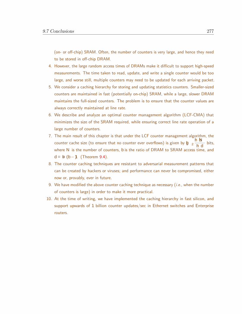
9.7 Conclusions 277
(on- or off-chip) SRAM. Often, the number of counters is very large, and hence they need
to be stored in off-chip DRAM.
4. However, the large random access times of DRAMs make it difficult to support high-speed
measurements. The time taken to read, update, and write a single counter would be too
large, and worse still, multiple counters may need to be updated for each arriving packet.
5. We consider a caching hierarchy for storing and updating statistics counters. Smaller-sized
counters are maintained in fast (potentially on-chip) SRAM, while a large, slower DRAM
maintains the full-sized counters. The problem is to ensure that the counter values are
always correctly maintained at line rate.
6. We describe and analyze an optimal counter management algorithm (LCF-CMA) that
minimizes the size of the SRAM required, while ensuring correct line rate operation of a
large number of counters.
7. The main result of this chapter is that under the LCF counter management algorithm, the
counter cache size (to ensure that no counter ever overflows) is given by log2
ln bN
ln dbits,
where N is the number of counters, b is the ratio of DRAM to SRAM access time, and
d = b=(b− 1) (Theorem 9.4).
8. The counter caching techniques are resistant to adversarial measurement patterns that
can be created by hackers or viruses; and performance can never be compromised, either
now or, provably, ever in future.
9. We have modified the above counter caching technique as necessary (i.e., when the number
of counters is large) in order to make it more practical.
10. At the time of writing, we have implemented the caching hierarchy in fast silicon, and
support upwards of 1 billion counter updates/sec in Ethernet switches and Enterprise
routers.

Chapter 10: Maintaining State with Slower
MemoriesMay 2008, Santa Rosa, CA
Contents
10.1 Introduction . . . . . . . . . . . . . . . . . . . . . . . . . . . . . . . . 280
10.1.1 Characteristics of Applications that Maintain State . . . . . . . . . . . 284
10.1.2 Goal . . . . . . . . . . . . . . . . . . . . . . . . . . . . . . . . . . . . . 285
10.1.3 Problem Statement . . . . . . . . . . . . . . . . . . . . . . . . . . . . . 285
10.2 Architecture . . . . . . . . . . . . . . . . . . . . . . . . . . . . . . . . 286
10.2.1 The Ping-Pong Algorithm . . . . . . . . . . . . . . . . . . . . . . . . . 287
10.3 State Management Algorithm . . . . . . . . . . . . . . . . . . . . . . 288
10.3.1 Consequences . . . . . . . . . . . . . . . . . . . . . . . . . . . . . . . . 294
10.4 Implementation Considerations . . . . . . . . . . . . . . . . . . . . . 295
10.5 Conclusions . . . . . . . . . . . . . . . . . . . . . . . . . . . . . . . . . 297
List of Dependencies
• Background: The memory access time problem for routers is described in
Chapter 1. Section 1.5.2 describes the use of load balancing techniques to
alleviate memory access time problems for routers.
Additional Readings
• Related Chapters: The general load balancing technique called constraint sets,
used for analysis in this chapter, was first described in Section 2.3. Constraint sets
are also used to analyze the memory requirements of other router architectures
in Chapters 2, 3, 4 and 6.

Table: List of Symbols.
C Number of Updates per Time SlotE Number of State Entriesh Number of BanksM Total Memory BandwidthR Line RateS Speedup of MemoryT Time slot
TRC Random Cycle Time of Memory
Table: List of Abbreviations.
ISP Internet Service ProviderI/O Input-Output (Interconnect)GPP Generalized Ping-PongSMA State Management Algorithm
SRAM Static Random Access MemoryDRAM Dynamic Random Access Memory

“To ping, pong, or ping-pong?”
— The Art of Protocol Nomenclature† 10Maintaining State with Slower Memories
10.1 Introduction
Many routers maintain information about the state of the connections that they
encounter in the network. For example, applications such as Network Policing,
Network Address Translation [208], Stateful Firewalling [194], TCP Intercept, Network
Based Application Recognition [209], Server Load balancing, URL Switching, etc.,
maintain state. Indeed, the very nature of the application may mandate that the
router keep state.
The general problem of state maintenance can be characterized as follows: When a
packet arrives, it is first classified to identify the connection or flow (we will describe
this term shortly) to which it belongs. If the router encounters a new flow, it creates
an entry for that flow in a flow table and keeps a state entry in memory corresponding
to that flow. If packets match an existing flow, the current state of the flow is retrieved
from memory. Depending on the current state, various actions may be performed on
the packet — for example, the packet may be accepted or dropped, it may receive
expedited service, its header may be re-written, the packet payload may be encrypted,
or it may be forwarded to a special port or a special-purpose processor for further
†Ping is an application to troubleshoot networks. Pong is an internal Cisco proposal forsynchronizing router clocks (currently subsumed by IEEE 1588). Ping-pong is a technique that isgeneralized in this chapter to maintain state entries on slower memories.
280
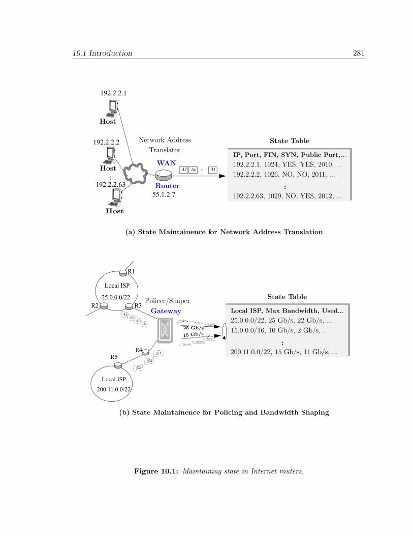
10.1 Introduction 281
Host
Network Address
WAN
Translator
Local ISP
25.0.0.0/22
Local ISP
200.11.0.0/22
Router
R1
R4R5
R3R2
Host
Host
..
192.2.2.1
55.1.2.7
192.2.2.2
192.2.2.63
IP, Port, FIN, SYN, Public Port,... State Table
192.2.2.1, 1024, YES, YES, 2010, ...192.2.2.2, 1026, NO, NO, 2011, ...
192.2.2.63, 1029, NO, YES, 2012, ...
..
Z1
Z2
Z3
A1A2
A3A4
Gateway Local ISP, Max Bandwidth, Used... State Table
25.0.0.0/22, 25 Gb/s, 22 Gb/s, ...
200.11.0.0/22, 15 Gb/s, 11 Gb/s, ...
..
15.0.0.0/16, 10 Gb/s, 2 Gb/s, ..
(a) State Maintainence for Network Address Translation
(b) State Maintainence for Policing and Bandwidth Shaping
25 Gb/s15 Gb/s
A2
Z1
Z2
Z3
A3A4
Policer/Shaper
A7 A6 A1..
Figure 10.1: Maintaining state in Internet routers.

10.1 Introduction 282
processing, etc. Once the action is performed, the state entry is modified and written
back to memory.
Example 10.1. Figure 10.1 shows two examples of routers maintaining state — (a)
A network address translator [208] keeps state for connections, so that
it can convert private IP addresses to its own public IP address when
sending packets to the Internet, (b) A gateway router belonging to a
backbone Internet service provider (ISP) maintains state for packets
arriving and departing from local ISPs, so that it can police data and
provide the appropriate bandwidth based on customer agreements and
policy.
We are not concerned with how the various flows are classified and identified, or the
actions that are performed on the packet once the state entry is retrieved. The task
of flow classification is algorithmic in nature, and a number of techniques have been
proposed to solve this problem [134, 184]. Similarly, the actions that are performed
on the packet (after the state entry is retrieved) are compute-intensive and are not
a focus of this chapter. We are only concerned with how the actual state entry is
updated because the operation is memory-intensive.
NObservation 10.1. A flow is defined by the specific application that maintains
state. The granularity of a flow can be a single connection or a set of
aggregated connections. For example, a network address translator, a
stateful firewall, and an application proxy maintain flow state entries
for each individual TCP/UDP connection they encounter. A policer,
on the other hand, may keep state entries at a coarser level — for
example, it may only maintain state entries for all packets that match
a certain set of pre-defined policies or an access control list.
In summary, a state entry needs to be read, modified, and written back to memory
in order to update its state. This operation is usually referred to as a “read-modify-
write” operation. The set of tasks required to perform state maintenance is shown

10.1 Introduction 283
Read
..
..
..
..
CAM (Classification)
TIME, SYN, FIN, ACK, MIN, MAX, MARK
...
State Memory
1
2
N
3
250001, YES, NO, YES, 0640, 10016, NONE
220105, YES, NO, NO, 0064, 09016, NONE
000105, YES, YES, YES, 0040, 01024, NONE
..
State Memory
IdentifyFlows Flow
..
R’
R’R’R’ Extract
Headers
Switch Fabric
WriteFlow
PacketMake Decision
R
Flow Address
250001, YES, NO, YES, 0640, ...
2508
90, Y
ES,
YES,
YES,
012
0, ..
.
Figure 10.2: Maintaining state on a line card.

10.1 Introduction 284
in Figure 10.2. As we will see, the rate at which state entries can be updated is
bottlenecked by memory access time. It is our goal to study and quantitatively analyze
the problem of maintaining state entries [210]. We were not aware of any previous
work that describes the problem of maintaining state entries at high speeds. And so
we are motivated by the following question — How can we build high-speed memory
infrastructure for high-speed routers, particularly when the updates need to occur faster
than the memory access rate?
10.1.1 Characteristics of Applications that Maintain State
We are interested in a general solution (which does depend on the characteristics of
any one particular application) that can maintain state entries at high speeds. The
applications that our solution must cater to share the following characteristics:
1. Our applications maintain a large number of state entries, one for each flow. For
example, a firewall keeps track of millions of flows, while an application proxy
usually tracks the state of several hundreds of thousands of connections. These
applications require a large memory capacity, making it unfeasible (or at least
very costly) to store them on-chip in SRAM. Instead, it becomes necessary to
store the state entries in off-chip memory.
2. Our applications update their state entries frequently, usually once for each
packet arrival. In the worst case, they must keep up with the rate at which the
smallest-sized packets can arrive.
3. Our applications are sensitive to latency. This is because the packets in our
applications must wait until the state entry is retrieved before any action
can be performed. So our solution should not have a large memory latency.
More important, the latency to retrieve a state entry must be predictable and
bounded. This is because packet processing ASICs often use pipelines that are
several hundred packets long – if some pipeline stages are non-deterministic, the
whole pipeline can stall, complicating the design. Second, the system can lose
throughput in unpredictable ways.

10.1 Introduction 285
4. Our applications mandate that state entries be updated at line rate. There must
be no loss of performance, and no state entry must be left unaccounted for.
10.1.2 Goal
Our goal is to build a memory subsystem that can update state entries at high speeds
that make no assumptions about the characteristics of the applications or the traffic.
Indeed, similar to the assumptions made in Chapter 7, we will mandate that our
memory subsystem give deterministic performance guarantees and ensure that we
can update entries at line rates, even in the presence of an adversary. Of course, it is
also our goal that the solution that caters to the above applications can update state
entries at high speeds with minimum requirements on the memory.
NObservation 10.2. Routers that keep measurement counters (as described in Chap-
ter 9) also maintain state. Thus, the storage gateway, the central
campus router, the local bridge, and the gateway router in Figure 9.1
may all maintain state. Conceptually there are two key differences
between applications that keep state and applications that maintain
statistics counters — (1) Applications do not need the value of the
measurement counter (and hence do not need to retrieve the counter)
for each packet, and (2) Counting is a special transformation of the data
(i.e., depending on the way counters are stored and their value, only a
few bits are modified at a time), whereas a state-based application can
transform the read value in a more general manner.
10.1.3 Problem Statement
The task of state maintenance must be done at the rate at which a smallest-size packet
can arrive and depart the router line card. For example, with a line rate of 10 Gb/s,
a “read-modify-write” operation needs to be done (assuming 40-byte minimum-sized
packets) once every 32 ns. Since there are two memory operations per packet, the
memory needs to be accessed every 16 ns. This is already faster than the speed of the

10.2 Architecture 286
most widely used commodity SDRAM memories, which currently have an access time
of ∼50 ns. It is extremely challenging to meet this requirement because, unlike the
applications that we described in the previous chapters (packet buffering, scheduling,
measurement counters, etc.), there is no structure that can be exploited when updating
a state entry. Indeed, any state entry can be updated (depending on the packet that
arrived). The memory subsystem must cater to completely random accesses. Further,
as line rates increase, the problem only becomes worse.
Example 10.2. At 100 Gb/s, a 40-byte packet arrives in 3.2 ns, which means
that the memory needs to be accessed (for a read or a write) every
1.6ns. This is faster than the speed of the highest-speed commercial
QDR-SRAM [2] available today.
10.2 Architecture
In what follows, we will first describe the main constraint in speeding up the memory
update rate in a standard memory, and then describe techniques to alleviate this
constraint. We note that read-modify-write operations involve two memory accesses —
(1) the state entry is read from a memory location, and (2) then later modified and
written back. Since the state entry for a particular flow resides in a fixed memory
location, both the read and write operations are constrained, i.e., they must access
the same location in memory.
In order to understand how memory locations are organized, we will consider a
typical commodity SDRAM memory. An SDRAM’s internal memory is arranged
internally as a set of banks. The access time of the SDRAM (i.e., the time taken
between consecutive accesses to any location in the memory) is dependent on the
sequence of memory accesses. While there are a number of constraints on how the
SDRAM can be accessed (see Appendix A for a discussion), the main constraint is
that two consecutive accesses to memory that address the same bank must be spaced
apart by time TRC (which is called the random cycle time of the SDRAM). However,
if the two consecutive memory accesses belong to different banks, then they need to

10.2 Architecture 287
be spaced apart by only around TRR time (called the cycle time of DRAM when there
is no bank conflict).
Unfortunately, the bank that should be accessed on an SDRAM depends on where
the state entry for the corresponding flow to which an arriving packet belongs is stored.
Since we do not know the pattern of packet arrivals, the bank that is accessed cannot
be predicted a priori. In fact, for any particular state entry, the read and the write
operations must access the same bank (because they access the same entry), preventing
consecutive memory operations from being accessed any faster than TRC time. Since
designers have to account for the worst-case memory access pattern, the state entries
can be updated only once in every two random cycle times in any commodity DRAM
memory.
NObservation 10.3. In general for any SDRAM, TRR < TRC , and so if one could
ensure that consecutive accesses to DRAM are always made to different
banks, then one can speed up the number of accesses that an SDRAM
can support by accessing it once every TRR time. On the other hand,
if these memory banks were completely independent (for example, by
using multiple physical DRAMs, or if the memory banks were on-chip),
and we could ensure that consecutive memory accesses are always to
different banks, then depending on the number of banks available, we
could potentially perform multiple updates per TRC time.
10.2.1 The Ping-Pong Algorithm
How can we ensure that consecutive memory accesses do not access the same bank?
Consider the following idea:
DIdea. We can read the state from a bank that contains an entry, and write it
back to an alternate bank that is currently not being accessed.

10.3 State Management Algorithm 288
Indeed, the above idea is well known and is referred to in colloquia as the “ping-
pong” or “double buffering” algorithm [211, 212]. The technique is simple — a read
access to an entry, and a write access to some other entry, are processed simultaneously.
The read access always gets priority and is retrieved from the bank that contains the
updated state entry. If the write accesses the same bank as the read, then it is written
to an alternate bank. Thus every entry can potentially be maintained in one of two
banks. A pointer is maintained for every entry, to specify the bank that contains the
latest updated version of the state entry.
NObservation 10.4. Note that instead of a pointer, a bitmap could be maintained to
specify which of the two banks contains the latest updated version of
the entry. Only one bit per entry is needed to disambiguate the bank.
In contrast, a pointer-based implementation that allocates a state entry
to an arbitrary new location (when it updates the state entry) requires
log 2E bits per entry, where E is the total number of state entries. Of
course, in order to maintain bitmaps, when a state entry is written to
a bank, it must be written to a memory address that is the same as
its previous address, except that it is different in the most significant
bits that represent the bank to which it is written. Note that with
the above technique, the memory update rate can be speeded up by a
factor of two, at the consequence of losing half the memory capacity.
10.3 State Management Algorithm
The ping-pong technique can speed up state updates by a factor of two. However, it
is not clear how we can extend the above algorithm to achieve higher speedup. The
problem is that the read accesses to memory are still constrained. We are looking for
a general technique that can be used to speed up the performance of a memory for
any value of the speedup S. This motivates the following idea:
10.3 State Management Algorithm 289
DIdea. We can remove the constraints on the read by maintaining multiple
copies of the state entry on separate banks, and alleviate the write constraints by
load balancing the writes over a number of available banks.
The above idea is realized in two parts.
1. Maintaining multiple copies to remove bank constraints on read ac-
cesses: In order to remove the read constraints on a bank, multiple copies of
the state entry are maintained on different banks. Depending on the banks that
are free at the time of access, any one of the copies of the state entry is read
from a free bank.
2. Changing the address and maintaining pointers to remove bank con-
strains on write accesses: When writing back the modified state entry, again
depending on the banks that are free, multiple copies of the modified state entry
are written to different banks, one to each distinct bank. Since the memory
location to the modified state entry changes, a set of pointers (or a bitmap as
described in Observation 10.4) to the multiple copies of the state entry for that
flow is maintained. Note that we need to maintain multiple copies of the updated
state entry, so that when the corresponding state entry is read (in future), the
read access has a choice of the banks to read the updated state entry from.
We will now formally describe a State Management Algorithm called “Generalized
Ping-Pong” (GPP-SMA) that realizes the above idea. Assume that GPP-SMA,
performs C read-modify-write operations every random cycle time, TRC . In what
follows, C is a variable, and we can design our memory subsystem for any value of C.
For GPP-SMA, C is also the number of copies of a state entry that must be maintained
for each flow. Clearly this is the case, since the C read accesses in a random cycle
time must all be retrieved from C distinct memory banks. GPP-SMA maintains the
following two sets.

10.3 State Management Algorithm 290
External Memory with Parallel Banks
Packet Processor/ASIC
0100100
0000011
0010001
1100000
...
Old location(s) for data
Old Bitmap State
Potential new location(s) for data
0100100
0000011
0010001
0000011...
New Bitmap State
One bit per bank for
1
2
N
each entry3
Figure 10.3: The read-modify-write architecture.
ℵDenition 10.1. Bank Read Constraint Set (BRCS): This is the set of banks
that cannot be used in the present random cycle time because a state
entry needs to be read from these banks. Note that at any given time
|BRCS| 6 C, because no more than C read accesses (one for each
of the C state entries that are updated) need to be retrieved in every
time period.
ℵDenition 10.2. Bank Write Constraint Set (BWCS): This is the set of banks
that cannot be used in the present random cycle time because data
needs to be written to these banks. During any time period, the
state entry for up to “C” entries needs to be modified and written
back to memory. Since C copies are maintained for each state entry,
this requires C × C = C2 write accesses to memory. All these C2
write accesses should occur to C2 distinct banks (as each bank can be
accessed only once in a time period). Hence |BWCS| 6 C2.
Figure 10.3 describes the general architecture, and how state entries are moved
from one bank to another after they are updated. We are now ready to prove the

10.3 State Management Algorithm 291
Algorithm 10.1: The Generalized Ping-Pong SMA.
input : Requests for Memory Updates.1
output: A bound on the number of memories and total memory bandwidth2
required to accelerate memory access time.
C ← Number of updates per random cycle time3
U ← (1, 2, . . . , h) /* Univeral set of all banks */4
for each time period T do5
BRCS ← ∅6
BWCS ← ∅7
for each read update request to entry e do8
/* Retrieve set of all banks for entry e */9
AvailableBanks ← RetrieveBanks(e) \ BRCS10
/* Choose bank and read entry */11
b ← AnyBank(AvailableBanks)12
Read entry e from bank b13
/* Update Bank Read Constraint Set */14
BRCS ← BRCS ∪ b15
for each write update request to entry e do16
/* Choose C banks for every entry */17
B1, B2, . . . BC ←PickBanksForWrite(U \BRCS \BWCS)18
Write entry e to chosen C banks B1, B2, . . . BC19
/* Update Bank Write Constraint Set */20
BWCS ← BWCS ∪ B1, B2, . . . BC21
/* Update bitmap for entry e */22
UpdateBankBitmap(e, B1, B2, . . . BC)23
main theorem of this chapter:
Theorem 10.1. (Sufficiency) Using GPP-SMA, a memory subsystem with h inde-
pendent banks running at the line rate can emulate a memory that can be updated at
C times the line rate (C reads and C writes), if C 6 b√
4h+1−1c2
.
Proof. In order that all the C reads and C2 writes are able to access a free bank, we
need to ensure that GPP-SMA has access to at least C + C2 = C(C + 1) banks. In

10.3 State Management Algorithm 292
Fraction of Memory Capacity Available
Upd
ate
Spee
dup
0
1
2
3
4
5
6
7
8
9
10
1 2 3 4 5 6 7 8 9 10 11 12 13 14 15 16 17 18 19 20
f h( ) 4h 1+ 1–=
(h=6, S=4)
(h=12, S=6). ..(h=2, S=2)
(h=20, S=8).
Figure 10.4: Tradeoff between update speedup and capacity using GPP-SMA.
any given time period, GPP-SMA first satisfies all the read accesses to memory. If
we have at least C banks, then clearly it is possible to satisfy this and read from C
unique banks, because each state entry is kept on C unique banks. However, we need
more banks. The remaining C2 writes must be written to C2 distinct banks (which
are distinct from the banks that were used to read C entries in the same random cycle
time). Hence, there need to be at least h > C +C2 independent banks. Solving for C,
we get,
C 6b√
4h+ 1 − 1c2
. (10.1)
Note that our analysis assumes that up to C banks are independently addressable
in the random cycle time of the memory.1 This completes the proof. r
1Commercial DRAM memories limit the maximum number of banks that can be addressed byany single chip in a given random cycle time, due to memory bandwidth limitations. This limit canbe increased by using multiple DRAM devices. Of course, if the memory banks are on-chip this isnot an issue.

10.3 State Management Algorithm 293
Box 10.1: Adversary Obfuscation
A large portion of the cost (in terms of memory bandwidth, cache size, etc.) ofdeploying the memory management algorithms described in this thesis comes from havingto defend against worst-case attacks by an adversary. In certain instances, the cost ofimplementing these algorithms may be impractical, e.g., they may require too many logicgates, or use a cache size too large to fit on packet processing ASICs. We could reduce thiscost (e.g., our algorithms could be simplified, or the caches can be sized sub-optimally),if we could somehow prevent worst-case adversarial attacks or bound the probability ofworst-case adversarial attacks.
In order to achieve this, we have deployed and re-used in multiple instances [33] (andthis has also been proposed by other research [204] and development groups [213]) an ideacalled adversary obfuscation. The basic technique is simple —
DIdea. “If the first access or value (e.g., addresses, block offsets, initialization values) ina sequence of operations that manipulate the data structures of the memory managementalgorithms can be obfuscated, then the relation between an adversarial pattern and the
state of the memory management algorithm cannot be deterministically ascertained”.
For example, the above idea can be implemented by randomizing the firsta access(or value) used by certain data structures, by the use of a programmable seed that isnot available to the adversary at run-time. Adversary obfuscation can be overlaid onmany of our deterministic memory management techniques to reduce the probability of anadversarial attack to a pre-determined low probability that is acceptable in practice (forexample, reducing the chance that an adversary is successful to less than 1 in 1030 tries).
NObservation 10.5. Note that adversary obfuscation is a natural consequence of theGPP-SMA algorithm. Every time a new entry is added, or an existing entryupdated, there is a natural choice of (a subset of h) banks that the newentry must be written to, C times. Since this choice is made at run-time,an adversary cannot predict the banks on which an updated entry is located.Over time, GPP-SMA exercises choice in every time slot, and the probabilityof an adversarial pattern becomes statistically insignificant.b
aThis can also be done periodically rather than just at the first access.bOf course, the function that exercises this choice can itself be seeded by a programmable
value created at run-time, and hence not available to the adversary.

10.3 State Management Algorithm 294
Figure 10.4 shows how GPP-SMA trades off update speedup with capacity. Note
that by definition the update speedup S = 2C, because with a standard memory
only one state entry can be updated every 2 random cycle times, whereas GPP-SMA
performs C updates per random cycle time.
From the above analysis, only the even Diophantine2 solutions for h and Diophantine
solutions for C that satisfy Equation 10.1 are true solutions.3 For example, only the
following values of (h,C) = (2, 1), (6, 2), (12, 3) . . . are valid. This is because the above
analysis assumes that C updates are performed in a time period TRC , where C is
assumed to be an integer. But if we are interested in non-integer values of C (for
example, C = 2.5 updates per random cycle time), we could do the above analysis
over a different time period which is a multiple of TRC , say yTRC , such that yC is
an integer. Then it is possible to find non-integer values of C. This will result in a
tighter bound for the number of banks required to support non-integer values of C.
In practice, non-integer values of C are almost always required.
Example 10.3. Consider a 10 Gb/s line card with a state table of size 1 million
entries, which are 256 bits in width. Suppose that a minimum-sized
packet is 40 bytes, and so it arrives once every 32 ns. The state entries
need to be updated once every 32 ns. Suppose we used a 1 Gb DRAM
that has a random access time TRC = 50 ns (i.e., and so can be
updated once every 100 ns, i.e., over three times slower than the rate
that is required). Then GPP-SMA, with a DRAM having 4 independent
banks, can speed up the memory subsystem to update an entry every
25 ns (such that the DRAM has a capacity of 256 Mb), which is good
enough for our purposes.
10.3.1 Consequences
We consider a number of consequences of the GPP-SMA algorithm.
2The term Diophantine refers to integer solutions.3This is because for any value of C, we need h = C(C + 1) banks, which is always an even
number.

10.4 Implementation Considerations 295
1. Special case for Read Accesses: If state entries are only read (but not
modified), then only the first part of GPP-SMA (i.e., maintaining multiple
copies of the state entries) needs to be performed when a state entry is created.
In such a case, GPP-SMA degenerates to an obvious and trivial algorithm where
state entries are replicated across multiple banks to increase the read access rate
supported by the memory subsystem.
2. Special case for the Ping-Pong Algorithm: Note that a special case for
GPP-SMA (Algorithm 10.1), with h = 2 and C = 1, leads to the ping-pong
algorithm described in Section 10.2.1. Since C = 1, no copies need to be
maintained. In such a case, only the second part of the GPP-SMA algorithm
(i.e., load balancing the write accesses) needs to be performed.
3. Applicability to Other Applications: GPP-SMA makes no assumptions
about the memory access pattern. It is orthogonal to the other load balancing
and caching algorithms described throughout this thesis. And so, it can be used
in combination with these techniques.
Example 10.4. For example, GPP-SMA with h banks can be applied in combination
with the buffer and scheduler caching algorithms described in Chapters 7
and 9 respectively to reduce their cache size by a factor of√h .
10.4 Implementation Considerations
We consider a number of implementation-specific considerations and optimizations for
GPP-SMA.
1. Optimizing the Data Structure: It is easy to implement GPP-SMA in
hardware. For every memory access, the bank that contains the latest updated
version of the state entry needs to be accessed. This can be done by maintaining
C pointers to the C location(s) where the most updated version of the state
entry is maintained. But if the memory addresses used for the “C” copies of a
flow’s state entry, which are on “C” different banks, are kept identical (except

10.4 Implementation Considerations 296
for the bank number, which is different), then C separate pointers need not be
maintained. We only require a bitmap of size C(C+ 1) bits per entry to describe
which C of the possible C(C + 1) banks have the latest updated version of the
state entry for that particular entry. This reduces the size required to implement
GPP-SMA.
2. Using DRAM Bandwidth Eciently: GPP-SMA can be analyzed for a
time period of yTRC . In such a case, each bank can be accessed up to y times in
a time period of yTRC . When data is written back to a bank, multiple writes
to that bank can be aggregated together and written to contiguous memory
locations in an efficient manner.4 This allows GPP-SMA to utilize the DRAM
I/O bandwidth efficiently.
3. Saving I/O Write Bandwidth: GPP-SMA performs C updates per random
cycle time and creates C copies for each update, for a total of C2 writes per
random cycle time. If the copy function was done in memory, or if the memory
was on-chip, there would be no need to carry each of the C2 writes on the memory
interconnect. With a copy function in memory, the number of distinct write
entries that are carried over the interconnect would reduce to C per random
cycle time. This would save memory I/O bandwidth, reduce the number of
ASIC-to-memory interface pins, and reduce worst-case I/O power consumption.
Indeed, with the advent of eDRAM [26]-based memory technology (which is
based on a standard ASIC process), it is relatively easy to create memory logic
circuitry that is capable of copying data over multiple banks.
4. Scalability and Applicability: GPP-SMA requires h banks (and hence only
gives 1h
of the memory capacity) in order to be able to speed up the updates by
a factor of Θ(√h ). Clearly, this is not very scalable for large values of speedup
unless the memory capacity is very large. Based on current technology constraints
and system requirements, we have noticed that GPP-SMA is practical for small
values of speedup (S 6 4). As the capacity of memory improves (roughly at the
4DRAM memories are particularly efficient in transferring large blocks of data to consecutivelocations. This is referred to as burst mode in DRAM. Refer to Appendix A for a discussion.

10.5 Conclusions 297
Table 10.1: Tradeoffs for memory access rate and memory capacity.
Banksper Entry
#Updates perTimeSlot
Memory AccessRate Speedup
TotalMemory
BandwidthComment
h C S M ≡ C + C2 -
1 0.5 1 11 update in 2
TRC ’s
2 1 2 21 update per
TRC
4 1.33 2.67 44 updates in 3
TRC ’s
5 1.5 3 4.53 updates in 2
TRC ’s
6 2 4 62 updates per
TRC
12 3 6 123 updates per
TRC
h C 6 b√
4h+1−1c2
S 6 b√
4h+ 1 − 1c M 6 hC updates per
TRC
speed of Moore’s law), higher values of update speedup may become practical,
as more memory banks per area can be fitted on-chip.
NObservation 10.6. The advent of on-chip memory technology such as eDRAM [26]
has allowed ASIC designers the flexibility to structure memory banks
based on their application requirements. Today, it is not uncommon to
have h > 32 banks with eDRAM-based memory.5
Table 10.1 summarizes the performance of GPP-SMA, and describes the tradeoff
between the number of banks used, and the update speedup.
10.5 Conclusions
A number of data-path applications on routers maintain state. We used the “constraint
set” technique (first described in Chapter 2) to build a memory subsystem that can
be used to accelerate the perceived random access time of memory. An algorithm
called GPP-SMA was described which can speed up memory by a factor Θ(√h ),
where h is the number of banks that a state entry can be load balanced over. Our
5As an example, Cisco Systems builds its own eDRAM-based memories [32] that have densities,capacities, and number of banks that cater to networking-specific requirements.

10.5 Conclusions 298
algorithm makes no assumptions on the memory access pattern. The technique is easy
to implement in hardware, and only requires a bitmap of size h bits for each entry, to
be maintained in high-speed on-chip memory. The entries themselves can be stored
in main memory (for example, commodity DRAM) running Θ(√h ) slower than the
line rate. For example, a state table of size ∼ 160 Mb, and capable of updating 40 M
updates/sec, can be built from DRAM that allows up to 6 banks to be independently
addressed in a random cycle time, with capacity 1 Gb and a TRC of 50 ns (which
could have supported no more than 10 M updates/s on its own).
Our technique has two caveats — (1) The DRAM capacity lost in order to speed
up the random cycle time grows quadratically as a function of the speedup, limiting
its scalability, and (2) The technique requires larger memory bandwidth.
While there are systems for which the above technique cannot be applied (e.g.,
systems that require extremely large speedup), we have seen that these techniques are
practical for small values of speedup (S 6 4). While we have not used these techniques
for current-generation 40 Gb/s line cards (mainly due to the use of eDRAMs [26] which
were able to meet the random cycle time requirements at 40 Gb/s), we are currently
negotiating deployment of the above technique for the next-generation 100 Gb/s
Ethernet switch and Enterprise router line cards, where even eDRAM can be too slow
to meet the random cycle time requirements.
Summary
1. A number of data-path applications on routers maintain state. These include: stateful
firewalling, policing, network address translation, etc.
2. The state maintained is usually to track the status of a “flow”. The granularity of a
flow can be coarse (e.g., all packets destined to a particular server) or fine (e.g., a TCP
connection), depending on the application.
3. When a packet arrives, it is first classified, and the flow to which it belongs is identified.
An entry in the memory (to which the flow belongs) is identified. Based on the packet,
some action is performed, and later the entry is modified and written back. This is referred
to as a “read-modify-write” operation.

10.5 Conclusions 299
4. However, the large random access times of DRAMs make it difficult to support high-speed
read-modify-write operations to memory.
5. We consider a load balancing algorithm that maintains copies of the flow state in multiple
locations (banks) in memory. The problem is to ensure that irrespective of the memory
access pattern, flow state entries can be read and updated faster than the memory access
rate of any single memory bank.
6. We describe and analyze a state management algorithm called “generalized ping-pong”
(GPP-SMA) that achieves this goal.
7. The main result of this chapter is that the generalized ping-pong algorithm, with h indepen-
dent memory banks running at the line rate, can emulate a memory that can be updated
at C times the line rate (C reads and C writes), if C 6 b√
4h+1−1c2 (Theorem 10.1).
8. GPP-SMA is resistant to adversarial memory accesses that can be created by hackers or
viruses; and its performance can never be compromised, either now, or provably, ever in
future.
9. GPP-SMA requires a small bitmap to be maintained on-chip to track the entries maintained
in DRAM, and is extremely practical to implement.
10. GPP-SMA can speed up the memory access time of any memory subsystem. Hence the
technique is orthogonal to the various load balancing and caching techniques that are
described in the rest of this thesis. Thus it can be applied in combination with any of the
other memory management techniques. For example, it can reduce the cache sizes of the
packet buffering and scheduler caches described in Chapters 7 and 8.
11. The main caveat of the technique is that it trades off memory capacity for random cycle
time speedup, and requires additional memory bandwidth, and so its applicability is usually
limited to low values of speedup (S 6 4).
12. At the time of writing, we are considering deployment of these techniques for the next
generation of 100 Gb/s Ethernet switch and Enterprise router line cards.

Chapter 11: ConclusionsJune 2008, San Francisco, CA
Contents
11.1 Thesis of Thesis . . . . . . . . . . . . . . . . . . . . . . . . . . . . . . 301
11.2 Summary of Contributions . . . . . . . . . . . . . . . . . . . . . . . . 301
11.3 Remarks Pertaining to Industry . . . . . . . . . . . . . . . . . . . . 302
11.4 Remarks Pertaining to Academia . . . . . . . . . . . . . . . . . . . . 304
11.4.1 Spawning New Research . . . . . . . . . . . . . . . . . . . . . . . . . . 305
11.5 Closing Remarks . . . . . . . . . . . . . . . . . . . . . . . . . . . . . . 306
11.5.1 Limitations and Open Problems . . . . . . . . . . . . . . . . . . . . . 306
11.5.2 Applications Beyond Networking . . . . . . . . . . . . . . . . . . . . . 307
11.5.3 Ending Remarks . . . . . . . . . . . . . . . . . . . . . . . . . . . . . . 308
You cannot simply cross the Bay Area on a whim. San Francisco Bay, more than 1600 square miles
in size, neatly bisects the area in two separate halves. A series of freeways with toll booths connect the
Peninsula and East Bay. For a picturesque crossing, you can take the Golden Gate Bridge at the mouth of
the Bay, one of the world’s largest suspension bridges, considered a marvel of engineering when it was
built in 1937.
However, if you want to avoid the toll ($5 if you are well-behaved) and are in a mood to inspect more
recent engineering wonders, take the turnoff to Highway 237 at the Bay’s opposite end. The freeway
begins in Mountain View, home of Google, a small company specializing in niche search engine technology
(we suggest you look them up). If you’re not in a rush, take the last exit. You’ll soon find yourself in a
large campus with buildings that all look alike, the home of a networking systems vendor. Bear right on
Cisco Way, and you’ll see an inconspicuous sign — “Datacenter Networked Applications (DNA) lab, Cisco
Systems”.
Unlike its large, frugal setting, the DNA lab is small and holds an expensive assemblage of the
highest-speed Ethernet switches and Enterprise routers, including storage equipment, high-performance
computing systems, disk arrays, and high-density server farms. These products are placed neatly side by
side to showcase the next-generation, high-speed data center networking technologies. Glance around and
you’ll see a large array of overhead projectors, and walls adorned with ∼20+ onscreen displays. Go ahead,
look around and experience the tremendous speed and capabilities of these modern engineering marvels.
Be sure to ask a network expert for a demo. Legend has it that if you look carefully, you’ll find (tell us if
you do) a nondescript sticker on each router: “High-speed router — fragile, handle with care. . . ”
“If you are afraid of change, leave it here”.
— Notice on a Tip Box†
“Make everything as simple as possible, but not simpler”.
— Albert Einstein‡ 11Conclusions
11.1 Thesis of Thesis
The thesis of this thesis is two-pronged, with one prong pertaining to industry and
the other to academia —
1. We have changed the way high-speed routers are built in industry, and we have
showed that (a) their performance can be scaled (even with slow memories), (b)
their memory subsystems need not be fragile (even in presence of an adversary,
either now or, provably, ever in future) and (c) they can give better deterministic
memory performance guarantees.
2. We have contributed to, unified, and, more important, simplified our understand-
ing of the theory of router architectures, by introducing (and later extending) a
powerful technique, extremely simple in hindsight, called “constraint sets”, based
on the well-known pigeonhole principle.
11.2 Summary of Contributions
Note 11.1. A summary of the 14 key results of this thesis is available in Section 1.11.
For more details on (1) the specific problems solved in this thesis, refer
to Section 1.7; and for (2) the industry impact and consequences of
these ideas, see Section 1.9; and (3) for a list of academic contributions
†Unknown Cafe, Mountain View, CA, Oct 2004.‡An obscure scientist of the early twentieth century.
301

11.3 Remarks Pertaining to Industry 302
that unify our understanding of the theory of router architectures, refer
to Table 2.1 and Section 2.3.
The next two sections discuss the impact of this thesis on industry and academia
respectively.
11.3 Remarks Pertaining to Industry
NObservation 11.1. Networking both reaps the boons and suffers the curses of
massive current deployment. This means that new ideas can make
a large impact, but that they have an extremely hard time gaining
acceptance. Deploying a new idea in existing networks can be technically
challenging, require cooperation among hosts in the network, and can
sometimes be economically infeasible to put in practice. Consequently,
we face the unfortunate reality that a large percentage of really good
ideas, in academia and industry, are never deployed in networking.
In that sense, we were fortunate, because our ideas pertain to the
networking infrastructure layer, i.e., routers, so their acceptance does
not need cooperation among existing routers.
Writing a thesis several years after finishing the main body of the research1 has
at least the benefit that we don’t need to predict the potential of our academic
work. At the time of writing, we have managed to add to the repertoire several new
research ideas relevant to this area, and most important we have brought these ideas
to fruition. However, their deployment has been by no means easy. It has been a
learning, challenging, and humbling experience.
Routers are complex devices — they must accommodate numerous features and
system assumptions, require backward compatibility, and have ever-changing require-
ments due to the advent of new applications and network protocols. This has meant
1I wouldn’t recommend this to new students — “all but dissertation” is not a pleasurable state ofmind.

11.3 Remarks Pertaining to Industry 303
that, in order to realize our techniques in practice, we have had to modify them, devise
and introduce new techniques, and fine-tune existing ones. Achieving these goals has
taken nearly four years and significant resources. In hindsight, it was important to
spend time in industry, understand the real problems, and solve them from an insider’s
framework. In the course of implementation, we have learned that designs are complex
to implement, and their verification is challenging.
Example 11.1. For example, the packet buffer cache (see Figure 7.3) has six
independent data paths, each of which can access the same data
structure within four clocks on 40 Gb/s line cards. This leads to data
structure conflicts, and requires several micro-architectural solutions to
implement the techniques correctly. Similarly, almost all our designs
have had to be parameterized to cater to the widely varying router
requirements of Ethernet, Enterprise, and Internet routers. The state
space explosion, to deal with massive feature requirements from different
routers, meant that these solutions take years and large collaborative
efforts to build and deliver correctly.
It is a good time to ask — Have we achieved the goals we set for ourselves at
the onset of this thesis? At the current phase of deployment, I believe that it is an
ongoing but incomplete success. At the time of this writing, we have largely met
our primary goals — to scale the memory performance of high-speed routers, enable
them to give deterministic guarantees, and alleviate their susceptibility to adversaries.
We have designed, evangelized, and helped deploy these techniques on a widespread
scale, and it is expected that up to 80% of all high-speed Ethernet switches and
Enterprise routers2 will use one or more instances of these technologies. We are also
currently deploying these techniques on the next generation of 100 Gb/s line cards
(for high-volume Ethernet, storage, and data center applications). However, our work
is still incomplete, because we have yet to cater to high-speed Internet core routers.
At this time, we are in discussions for deploying these ideas in those market segments
as well.2Based on Cisco’s current proliferation in the networking industry.

11.4 Remarks Pertaining to Academia 304
The secondary consequences of our work have resulted in routers becoming more
affordable – by reducing memory cost, decreasing pins on ASICs, and reducing the
physical board space. They have also enabled worst-case and average-case power
savings. In summary, our work has brought tremendous engineering, economic, and
environmental benefits.
Note 11.2. From a user’s perspective, a network is only good if every switch or router
(potentially from several different router vendors) in a packet’s path
can perform equally well, give deterministic guarantees, and be safe
from adversarial attacks. To that end, most of the ideas described
in this thesis were done at Stanford University, are open source, and
available for use by the networking community at large.
11.4 Remarks Pertaining to Academia
I will now touch on the academic relevance of this work, and comment separately on
load balancing and caching techniques. It is clear that the constraint set technique
introduced in this thesis (to analyze load-balanced router memory subsystems) sim-
plifies and unifies our understanding of router architectures. However, it also has an
interesting parallel with the theory of circuit switching.
NObservation 11.2. Note that router architecture theory deals with packets that can
arrive and be destined to any output (there are a total of NN combina-
tions), while circuit switches deal with a circuit-switched, connection-
based network that only routes one among N ! permutations between
inputs and outputs. In that sense, router architecture theory is a su-
perset of circuit switching theory [110]. However, circuit switch theory
and constraint sets both borrow from the same pigeonhole principle.
This points to an underlying similarity between these two fields of
networking. From an academic perspective, it is pleasing that the
technique of analysis is accessible and understandable even by a high
school student!

11.4 Remarks Pertaining to Academia 305
11.4.1 Spawning New Research
Our initial work has led to new research in both algorithms and architectural techniques
pertaining to a broader area of memory-aware algorithmic design. Some significant
contributions include — simplified caches using frame scheduling, VOQ buffering
caches [181], packet caching [182], lightweight caching algorithms for counters [202,
203, 204, 205], caching techniques to manage page allocation, and increased memory
reliability and redundancy [32].
NObservation 11.3. Our caches have had some interesting and unforeseen benefits.
L2 caches3 (which are built on top of the current algorithmic L1 caches)
have been proposed and are currently being designed to decrease average
case power [25]. Also, larger L1 caches have been implemented to
hide memory latencies and allow the use of complementary high-speed
interconnect and memory serialization technology [32]. The structured
format in which our L1 caches access memory also allows for the
creation of efficient memory protocols [214] that are devoid of the
problems of variable-size memory accesses, and avoid the traditional
“65-byte” problem and memory bank conflicts.
In the process of development, we have sometimes re-used well-known existing
architectural techniques, and have in some cases invented new ones to deal with complex
high-speed designs. For example, the architectural concepts of cache coherency, the use
of semaphores, maintaining the ACID [215] properties of data structures (which are
updated at extremely high rates), deep pipelining, and RAID [30] are all concepts that
we have re-used (and tailored) for high-speed routers. Similarly, we have re-applied
the ideas pertaining to adversary obfuscation (see Chapter 10) to many different
applications. While these concepts are borrowed from well-known systems ideas
in computer architecture [155], databases, and the like, they also have significant
differences and peculiarities specific to networking.
3These terms are borrowed from well known-computer architecture terminology [155].

11.5 Closing Remarks 306
NObservation 11.4. From an academic perspective, it is heartening that there is a
common framework of load balancing and caching techniques that are
re-used for different purposes. Also, router data path applications, for
the most part, have well-defined data structures, and so lend themselves
to simple techniques and elegant results. I believe that routers have
reached a semi-mature stage, and I hope that this thesis will convince
the reader that we are converging toward an end goal of having a
coherent theory and unified framework for router architectures.
11.5 Closing Remarks
11.5.1 Limitations and Open Problems
Based on my experience in the networking industry, I would like to divide the limitations
of the techniques presented in this thesis into three broad categories. I hope that this
will stimulate further research in these three areas.
1. Unusual Demands From Current Applications: There are additional
features that data path applications are required to support on routers, outside
their primary domain. In general, any features that break the assumptions
made by the standard data structures of these applications can place unexpected
demands on our memory management techniques, and make their implementation
harder, and sometimes impractical. For example, unicast flooding requires packet
order to be maintained among packets belonging to different unicast and unicast
flood queues. This usually doubles the size of data structures for the queue
caching algorithms. Similarly, dropping large numbers of packets back to back4
requires over-design of the buffer and scheduler cache; buffering packets received
in temporary non-FIFO order makes the implementation of the tail cache more
complex, and handling extremely small packets at line rates can cause resource
4Packets can easily be dropped faster than the line rate, because in order to drop a packet of anysize, only a constant-size descriptor needs to be dropped.

11.5 Closing Remarks 307
problems when accessing data structures. All of the above require special
handling or more memory resources to support them at line rates.
2. Scalability of Current Applications: The complexity of implementation of
our results (in terms of number of memories required, cache sizes, etc.) usually
depends on the performance of the memory available. While our techniques
are meant to alleviate the memory performance problem, and in theory, have
no inherent limitations, there are practical limits in applying these approaches,
especially when memories become extremely slow. Also, there are instances
where the feature requirements are so large that our techniques are impractical
to implement. As an example, some core routers require tens of thousands of
queues. Multicast routers require Θ(2f) queues, where f 6 q is the maximum
multicast fanout, and q is the number of unicast queues. The cache size needed
to support this feature is Θ(f ∗ 2f), which can be very large. Similarly, load
balancing solutions require a large (≡ Θ(√f )) speedup (refer to Appendix J) to
achieve deterministic performance guarantees for multicast traffic. This is an
area of ongoing concern that needs further improvement.
3. Unpredictability of Future Applications: Our caching and load balancing
solutions are not a panacea. The router today is viewed as a platform, and is
expected to support an ever-increasing number of applications in its data path.
These new applications may access memories in completely different ways and
place unforeseen demands on memory. We cannot predict these applications,
and new techniques and continued innovation will be necessary to cater to and
scale their performance.
11.5.2 Applications Beyond Networking
Our techniques exploit the fundamental nature of memory access. While the most
useful applications that we have found are for high-speed routers, their applicability
is not necessarily limited to networking. In particular, the constraint set technique
could be used wherever there are two (or more) points of contention in any load
balancing application, for example, in job scheduling applications. They can also
11.5 Closing Remarks 308
be used in applications that keep FIFO and PIFO5 queues. Similarly, our caching
techniques can be used in any application that uses queues, manipulates streams of
data, walks linked lists (e.g., data structures that traverse graphs or state tables, as
used in deterministic finite automata (DFA)), aggregates or pre-fetches blocks of data,
copies data, or measures events.
NObservation 11.5. Of course, the memory acceleration technique introduced in
this thesis can be used to speed up (by trading off memory capacity)
the random cycle time performance of any memory. The speedup is
by a factor, Θ(√h ), where h is the number of memory banks. This
points to an interesting and fundamental tradeoff. As memory capacity
increases at the rate of Moore’s law, we expect this to become a very
useful and broadly applicable technique. In addition, this technique is
orthogonal to the rest of the load balancing and caching techniques
described in this thesis, and so can be used in combination with these
various techniques to increase memory performance.
11.5.3 Ending Remarks
“Sufficiency is the child of all discovery”.
— Quick Quotations Corporation
As system requirements increase, the capabilities of hardware may continue to
lag. The underlying hardware can be slow, inefficient, unreliable, and perhaps even
variable and probabilistic in its performance. Of course, some of the above are already
true with regard to memory. And so, it will become necessary to find architectural
and algorithmic techniques to solve these problems. If we can discover techniques
that are sufficient to emulate the large performance requirements of the system, then
it is possible to build solutions that can use such imperfect underlying hardware. I
believe that such techniques will become more common in future, and are therefore a
continuing area of interest for systems research.
5This is defined in Section 1.4.2.

11.5 Closing Remarks 309
High-speed routers are complex devices. They function at the heart of the tremen-
dous growth and complexity of the Internet. While their inner workings can in some
instances be complex (and, like musical notation, the underlying mathematics can at
times be intimidating and can hide their inherent beauty), for the most part I hope
to have conveyed in this thesis that they are, in fact, quite simple, have a common
underlying framework, and lend themselves to elegant analysis. If a high school student
can appreciate this fact, I would consider the thesis successful.
Epilogue
Penning an epilogue is a pleasure. It’s not every day you can finish your thesis, polish
the last words, attend your advisor’s wedding in faraway Turkey, and sit back, relax,
and feel just a little bit satisfied. Yet I can’t help considering the irony! Academia
teaches us to think outside the box, but this thesis ponders ideas inside the box.
In the preface, I alluded to a need to refrain from social commentary. I lied. I was
attempting to put a finger on why I loved the Ph.D. process and the academic world.
Indulge me while I share my perspective.
In contrast to the world at large, which is inherently unfair and holds us responsible
for our moments of indecisiveness, irrationality, subjectivity, and prejudice, academic
thought is (in principle) rational, objective, and idealistic. There’s a certain utopian
aura, a purity and fairness connected with the scholarly life. It can give joys that
are (mostly) under your control, and even better, cannot be denied you. In many
cases, and this is definitely true of most mathematical and analytical research, the
only extremely portable tools you need are paper and pencil.6 Academic thought gives
you avenues to be creative, feel challenged, and keep your mind active and engaged.
Of course, one does experience frustration (e.g., nine-tenths of a proof is worth not
very much), but the genuine happiness of a handful of “Aha!” moments beats all the
hedonistic joys of the wider society.
I’m not trying to raise academia above society, but merely making some interesting
comparisons. This thesis, for example, tries to devise solutions for the Internet and
solve pressing problems of building high-speed networks. But, it pales in comparison to
the complexities of human networks.† What humans could learn from networked routers
is that routers communicate easily, are seldom offended, don’t mandate arbitrary
mores, and aren’t shy about sparking instant conversations.
While writing my thesis, I tried to be uncharacteristically asocial (because it helped
me concentrate). Yet over these ten months of writing, I’ve had many opportunities
6Of course, not a pen. They tend to leak when you are traveling to Mars : : :†. . . Sorry, Cisco, there really is only one human network!
310

to meet wonderful strangers, and collect their interesting anecdotes and amazing
experiences. These networking opportunities brought surprise benefits — complimen-
tary drinks, a lunch, several free dinners, a historical photo tour of Tiburon, a small
town just north of San Francisco, complementary museum tickets, a private showing
by a local artist, an invitation to go flying, a standing invitation to visit Malibu,
an invite from a Hollywood producer to visit the location for an advertising shoot,
introductions to interesting people and folksy advice in the kitschy small towns of
northern California. There were also some hilarious moments, aptly captured by an
old Turkish saying (perhaps you have heard it?), “What happens in Istanbul, stays in
Constantinople”.
And on that note, as I pen a roast on your wedding day, Asena and Nick, thank
you for a wonderful wedding, and here’s wishing you a long, happy, fulfilling, and —
what is that phrase? (see preface) — a stable marriage . . .
— Istanbul, Turkey,
July 11th 2008

Part III
Appendices & Bibliography
312

“Good, Fast, Cheap: Pick any two
(you can’t have all three)”.
— RFC 1925, The Twelve Networking Truths† AMemory Terminology
In this appendix, we will define some common terms related to memory. The two
most widespread memories available today are SRAM [2] and DRAM [3]. In what
follows, we will define the DRAM memory terminology, of which SRAM terms are a
subset.
A.1 Terminology
A DRAM’s memory array is arranged internally in rows, where a set of contiguous
rows form a bank. For example, Figure A.1 shows a DRAM with K banks, where
each bank has R rows. The four key memory terms of concern to us are:
1. Bandwidth: This refers to the total amount of data that can be transferred
from a single memory per unit time.
2. Capacity: This refers to the total number of bits that can be stored in the
memory.
3. Latency: This refers to the time it takes to receive data from memory, after a
request to access it has been issued by the requester.
†A more apt version for networking memories – “Dense, Fast, Cheap: Pick any two”.
313

A.1 Terminology 314
....
Sense Amp
A
..
Sense Amp
D
..
Sense Amp
E
..
Sense Amp
G
B
C
F
W R
Bank 1 Bank 2 Bank 3 Bank K
36
250 MHz, Dual Data Rate (DDR)
Row
s
Row 1
Row R
Figure A.1: Internal architecture of a typical memory.
4. Access Time: This refers to the minimum amount of time that needs to elapse
between any two consecutive requests to the memory. The memory access time
can depend on a number of factors, and this will be explained in the next section.
NObservation A.1. Note that the memory bandwidth is a function of three quantities
— (1) the data width of the memory, (2) the clock speed, and (3)
the number of edges used per clock to transfer data. For example, a
DRAM with a 36-bit data bus, running a 250 Mhz clock, which can
support dual-data rate (DDR) transfer (i.e., it can transfer data on
both edges of the clock) has a bandwidth of 36× 250× 2 = 18 Gb/s.

A.2 Access Time of a DRAM 315
A.2 Access Time of a DRAM
The access time T of the DRAM (i.e., the time taken between consecutive accesses to
any location in the memory array) is dependent on the sequence of memory accesses
made to the DRAM. These can be categorized as follows:
1. Consecutive cells in the same row and bank: The access time between
two consecutive references to adjacent memory locations in the same row of the
same bank is denoted by TC . This is sometimes referred to as the burst mode in
a DRAM. In Figure 2, consecutive references to cells A and B can be done in
burst mode. TC is usually about 5-10 ns today. Although this is fast, it is not
common in a router to be able to use burst mode, because successive cells do
not usually reside in the same row and bank.
2. Consecutive cells in dierent rows, but in the same bank: The access
time between two consecutive references to different rows but belonging to the
same bank is denoted by TRC . As an example, consider the consecutive references
to cells B and C in Figure A.1. We say that there is a bank conflict1 because
the rows being accessed belong to the same bank. TRC represents the worst-case
access time for random accesses to a DRAM, and it is of the order of 70-80ns
for commodity DRAMs available today.
3. Consecutive cells in adjacent banks: Some DRAMs such as RDRAM [7]
incur a penalty when two consecutive references are made to adjacent banks,
i.e., if a cell accesses bank x, then the next cell cannot access banks x− 1, x,
or x+ 1. This is called an adjacent bank conflict, and we will denote it by TAC .
This can occur if adjacent DRAM banks share circuitry, such as sense-amps.
As an example, consecutive references to cells D and E in Figure A.1 cause an
adjacent bank conflict. Most modern DRAMs do not share circuitry between
adjacent banks, and hence do not exhibit adjacent bank conflicts.
1This is also commonly called a row conflict, however this terminology is misleading, since it isthe banks that conflict, not the rows!

A.2 Access Time of a DRAM 316
4. Consecutive cells in dierent rows: The access time for two consecutive
references to rows in different banks is denoted by TRR and is called the row to
row access time. An example in Figure A.1 would be a reference to cell A, B, or
C followed by a reference to cell D. This number is of the order of 20ns and
usually represents the best-case random access time for a DRAM.
In a DRAM, there is usually a heavy penalty in the access time for a bank
conflict.2 Thus TRC TRR, TAC . In this thesis, when we mention random access
time, we will refer to the worst-case random access time of the DRAM, i.e., T =
maxTRC , TRR, TAC.
2Note that there can be other penalties such as the read-write turnaround and refresh penaltiesassociated with accesses to a DRAM.

“100% throughput? And the queue size
can still be any large value?”.
— The Art of Deceptive Definition† BDefinitions and Traffic Models
B.1 Denitions
In this thesis, we are interested in deterministic performance guarantees. However,
in some instances we refer to terms that are concerned with statistical performance
guarantees informally. We define these terms rigorously in this section.
We assume that time is slotted into cell times. Let Ai,j(n) denote the cumulative
number of arrivals to input i of cells destined to output j at time n. Let Ai(n) denote
the cumulative number of arrivals to input i. During each cell time, at most one cell
can arrive at each input. λi,j is the arrival rate of Ai,j(n). Di,j(n) is the cumulative
number of departures from output j of cells that arrived from input i, while Dj(n) is
the aggregate number of departures from output j. Similarly, during each cell time, at
most one cell can depart from each output. Xi,j(n) is the total number of cells from
input i to output j still in the system at time n. The evolution of cells from input i
to output j can be represented as:
Xi,j(n+ 1) = Xi,j(n) + Ai,j(n)−Di,j(n). (B.1)
Let A(n) denote the vector of all arrivals Ai,j(n), D(n) denote the vector of all
departures Di,j(n), and X(n) denote the vector of the number of cells still in the
†Stanford University, CA, 1999.
317

B.1 Definitions 318
A7A8
Switch Fabric
Z5Z9 Z6
...AN(n)
XN,N(n)
XN,1(n)
A4A5
Z4Z8 Z7
A1(n)
X1,N(n)
X1,1(n)
A1A2D1(n)
Z2Z3DN(n)
...
....
....
Inputs Outputs
Virtual Output Queues
Output Queues
Figure B.1: Network traffic models.
system. With this notation, the evolution of the system can be described as
X(n+ 1) = X(n) + A(n)−D(n). (B.2)
ℵDenition B.1. Admissible: An arrival process is said to be admissible when no
input or output is oversubscribed, i.e., when∑
i λi,j < 1,∑
j λi,j < 1,
λi,j ≥ 0.
ℵDenition B.2. IID: Traffic is called independent and identically distributed (iid) if
and only if:
1. Every arrival is independent of all other arrivals both at the same
input and at different inputs.
2. All arrivals at each input are identically distributed.

B.1 Definitions 319
ℵDenition B.3. 100% throughput: A router is said to achieve 100% throughput
if under any admissible iid traffic, for every ε > 0, there exists B > 0
such that
limn→∞
Pr∑i,j
Xi,j(n) > B < ε.

“It only takes a memory bandwidth of 3NR?
We had a bit more speedup than that : : : ”.
— Pradeep Sindhu† CProofs for Chapter 3
C.1 Proof of Lemma 3.1
Lemma 3.1. A request matrix can be ordered in no more than 2N − 1 alternating
row and column permutations.
Proof. We will perform the ordering in a iterative way. The first iteration consists of
one ordering permutation of rows or columns, and the subsequent iterations consist
of two permutations, one of rows and one of columns. We will prove the theorem by
induction.
1. After the first permutation, either by row or by column, the entry at (1, 1) is
non-zero, and this entry will not be moved again. We can define sub-matrices of
S as follows:
An = Sij|1 6 i, j 6 n,
Bn = Sij|1 6 i 6 n, n 6 j 6 N, (C.1)
Cn = Sij|n 6 i 6 N, 1 6 j 6 n.
2. If a sub-matrix of S is ordered and will not change in future permutations, we
call it optimal. Suppose An is optimal after the nth iteration. We want to prove
†Pradeep Sindhu, CTO, Juniper Networks.
320

C.2 Proof of Theorem 3.7 321
that after another iteration, the sub-matrix An+1 is optimal. Without loss of
generality, suppose a row permutation was last performed, then in this iteration,
we will do a column permutation followed by a row permutation. There are four
cases:
(a) The entries of Bn and Cn are all zeros. Then Sn+1,n+1 > 0 after just one
permutation, so the sub-matrix An+1 is optimal.
(b) The entries of Bn are all zeros, but those of Cn are not. After the column
permutation, suppose Sm,n+1(m > n) is the first positive entry in column
n + 1, then the first m rows of S are ordered and will remain so. Thus,
column n+ 1 will remain the biggest column in Bn, and An+1 is optimal.
(c) The entries of Cn are all zeros, but those of Bn are not. This case is similar
to case (b).
(d) The sub-matrices Bn and Cn both have positive entries. The column
permutation will not change row n+ 1 such that it becomes smaller than
the rows below it. Similarly, the row permutation following will not change
column n+ 1 such that it becomes smaller than the columns on its right.
So An+1 is optimal.
After at most N iterations, or a total of 2N − 1 permutations, the request matrix
is ordered. r
C.2 Proof of Theorem 3.7
Theorem 3.7. If a request matrix S is ordered, then any maximal matching algorithm
that gives strict priority to entries with lower indices, such as the WFA [15], can find
a conflict-free schedule.
Proof. By contradiction. Suppose the scheduling algorithm cannot find a conflict-free
time slot for request (m,n). This means
n−1∑j=1
Smj +m−1∑i=1
Sin > 4. (C.2)

C.2 Proof of Theorem 3.7 322
Now consider the sub-matrix S ′, consisting of the first m rows and the first n columns
of S. Let’s look at the set of the first non-zero entries of each row, Lr, and the set of
the first non-zero entries of each column, Lc. Without loss of generality, suppose S ′11
is the only entry belonging to both sets. (If this is not true, and S ′kl, where k 6= 1 or
l 6= 1, also belongs to both Lr and Lc, then we can remove the first k − 1 rows and
the first l − 1 columns of S ′ of to obtain a new matrix. Repeat until Lr and Lc only
have one common entry.) Then |Lr ∪ Lc| = m+ n− 1. At most two of the entries in
the mth row and those in the nth column are in Lr ∪ Lc, so the sum of all the entries
satisfies
∑i
∑j
Sij > (|Lr ∪ Lc| − 2) + Smn +n−1∑j=1
Smj +m−1∑i=1
Sin > 4. (C.3)
Hence we get, ∑i
∑j
Sij > m+ n+ 2, (C.4)
which conflicts with property 1 in Section 3.6. r

“You were proving this on a friday evening?
You need to go get a life!”.
— Da Chuang, Colleague Extraordinaire† DProofs for Chapter 5
In this appendix, we will prove that a buffered crossbar with a speedup of two
using arbitrary input and output scheduling algorithms achieves 100% throughput.
We will use the traffic models and definitions that were defined in Appendix B.
D.1 Achieving 100% Throughput in a Buered
Crossbar - An Outline
Figure D.1 shows the scheduling phases in a buffered crossbar with a speedup of two.
The two scheduling phases each consist of two parts: input scheduling and output
scheduling. In the input scheduling phase, each input (independently and in parallel)
picks a cell to place into an empty crosspoint buffer. In the output scheduling phase,
each output (independently and in parallel) picks a cell from a non-empty crosspoint
buffer to take from.
We know that the scheduling algorithm in a buffered crossbar is determined by
the input and output scheduling policy that decides how inputs and outputs pick cells
in the scheduling phases. The randomized algorithm that we considered in Chapter 5
to achieve 100% throughput was as follows:
†Da Chuang, Humorous Moments in Proof, Stanford, 2002.
323

D.1 Achieving 100% Throughput in a Buffered Crossbar - An Outline 324
Arrival DepartInput Output Input Output
Schedule-1 Schedule-1 Schedule-2 Schedule-2
Scheduling Phase I Scheduling Phase IIFigure D.1: The scheduling phases for the buffered crossbar. The exact order of the phasesdoes not matter, but we will use this order to simplify proofs.
Randomized Algorithm: In each scheduling phase, the input picks any non-
empty VOQ, and the output picks any non-empty crosspoint.
We will adopt the following notation and definitions. The router has N ports,
and V OQij holds cells at input i destined for output j. Xij is the occupancy of
V OQij,1 and Zij = Xij +Bij is the sum of the number of cells in the VOQ and the
corresponding crosspoint. We will assume that all arrivals to input i ∈ 1, 2, 3, ..., N
are Bernoulli i.i.d. with rate λi, and are destined to each output j ∈ 1, 2, 3, ...N with
probability λij. We will denote the arrival matrix as A ≡ [λij], where for all i, j,
λi =N∑j=1
λij, λj =N∑i=1
λij, 0 6 λij < 1. (D.1)
We will also assume that the traffic is admissible (see Definition B.1), i.e.,∑
i λi,j <
1,∑
j λi,j < 1. In what follows, we will show that the buffered crossbar can give 100%
throughput. The result is quite strong in the sense that it holds for any arbitrary
work-conserving input and output scheduling policy with a speedup of two. In other
words, each input i can choose to serve any non-empty VOQ for which Bij = 0, and
each output j can choose to serve any crosspoint for which Bij = 1.
First we describe an intuition and outline of the proof. Then, in the next section,
we will give a rigorous proof.
1We will see later that other queueing structures are useful and that it is not necessary to placecells in VOQs.

D.1 Achieving 100% Throughput in a Buffered Crossbar - An Outline 325
Theorem D.1. (Sufficiency) A buffered crossbar can achieve 100% throughput with
speedup two for any Bernoulli i.i.d. admissible traffic.
Proof. Intuition and Outline: For each V OQij , let Cij denote the sum of the cells
waiting at input i and the cells waiting at all inputs destined to output j (including
cells in the crosspoint for output j),
Cij =∑k
Xik +∑k
(Xkj +Bkj). (D.2)
It is easy to see that when V OQij is non-empty (i.e., Xij > 0), then Cij decreases
in every scheduling phase. There are two cases:
• Case 1: Bij = 1. Output j will receive one cell from the buffers destined to it,
and∑
k(Xkj +Bkj) will decrease by one.
• Case 2: Bij = 0. Input i will send one cell from its VOQs to a crosspoint, and∑kXik will decrease by one.2
With S = 2, Cij will decrease by two per time slot. When the inputs and outputs
are not oversubscribed, the expected increase in Cij is strictly less than two per time
slot. So the expected change in Cij is negative over the time slot, and this means that
the expected value of Cij is bounded. This in turn implies that the expected value of
Xij is bounded and the buffered crossbar has 100% throughput. r
2If a cell from V OQij is sent to crosspoint Bij , then∑
k(Xkj + Bkj) stays the same at the endof the input scheduling phase, since Xij decreases by one and Bij increases by one. In the outputschedule, Case 1 applies and Cij will further decrease by one. As a result, if a cell from V OQij issent to crosspoint Bij , then Cij decreases by two in that scheduling phase.

D.2 Achieving 100% Throughput in a Buffered Crossbar - A Rigorous Proof 326
D.2 Achieving 100% Throughput in a Buered
Crossbar - A Rigorous Proof
Lemma D.1. Consider a system of queues whose evolution is described by a discrete
time Markov chain (DTMC) that is aperiodic and irreducible with state vector Yn ∈ NM .
Suppose that a lower bounded, non-negative function F (Yn), called Lyapunov function,
F : NM → R exists such that ∀Yn, E[F (Yn+1)|Yn] <∞. Suppose also that there exist
γ ∈ R+ and C ∈ R+, such that ∀||Yn|| > C,
E[F (Yn+1)− F (Yn)|Yn] < −γ, (D.3)
then all states of the DTMC are positive recurrent and for every ε > 0, there exists
B > 0 such that limn→∞ Pr∑
i,j Xi,j(n) > B < ε.
Proof. This is a straightforward extension of Foster’s criteria and follows from [39,
216, 217, 218]. r
We will use the above lemma in proving Theorem D.1. We are now ready to prove
the main theorem, which we repeat here for convenience.
Theorem D.2. (Sufficiency) Under an arbitrary scheduling algorithm, the buffered
crossbar gives 100% throughput with speedup of two.
Proof. In the rest of the proof we will assume that all indices i, j, k vary from 1, 2, ..N .
Denote the occupancy of V OQij at time n by Xij(n). Also, let Zij denote the
combined occupancy of the V OQij and the crosspoint Bij at time n. By definition,
Zij(n) = Xij(n) +Bij(n).

D.2 Achieving 100% Throughput in a Buffered Crossbar - A Rigorous Proof 327
Define,
f1(n) =∑i,j
Xij(n)(∑
k
Xik(n)), (D.4)
f2(n) =∑i,j
Zij(n)(∑
k
Zkj(n)), (D.5)
F (n) = f1(n) + f2(n). (D.6)
Observe that from Equation D.4
f1(n) =∑i,j
Xij(n)(∑
k
Xik(n))
=∑i,j,k
Xij(n)Xik(n).
Denote Dij(n) = 1 if a cell departs from V OQij at time n and zero otherwise.
Also, let Aij(n) = 1 if a cell arrives to V OQij and zero otherwise. Then, Xij(n+ 1) =
Xij(n) + Aij(n)−Dij(n). Henceforth, we will drop the time n from the symbol for
Dij(n) and Aij(n), and refer to them as Dij and Aij respectively, since in the rest of
the proof, we will only be concerned with the arrivals and departures of cells at time
n.
Therefore, [f1(n+ 1)− f1(n)]
=∑i,j,k
[Xij(n+ 1)Xik(n+ 1)−Xij(n)Xik(n)]

D.2 Achieving 100% Throughput in a Buffered Crossbar - A Rigorous Proof 328
Then we get [f1(n+ 1)− f1(n)]
=∑i,j,k
(Xij(n) + Aij −Dij)(Xik(n) + Aik −Dik)−
Xij(n)Xik(n)
=∑i,j,k
(Aij −Dij)Xik(n) + (Aik −Dik)Xij(n)+
(Aij −Dij)(Aik −Dik)
=∑i,j,k
2(Aik −Dik)Xij(n) + (Aij −Dij)(Aik −Dik)
Since |Aij −Dij| ≤ 1 and similarly |Aik −Dik| ≤ 1, we get3
E[f1(n+ 1)− f1(n)] ≤ N3 +∑i,j,k
2E[Aik −Dik]Xij(n). (D.7)
Denote Eij(n) = 1 if a cell departs from the combined queue of V OQij and the
crosspoint Bij, and zero otherwise. Note that Eij(n) = 1 only when a cell departs
from the crosspoint Bij to the output at time n, since all departures to the output
must occur from the crosspoint. Also recall that the arrival rate to the combined
queue, V OQij and Bij, is the same as the arrival rate to V OQij. So we can write
Zij(n+ 1) = Zij(n) +Aij(n)−Eij(n). Again we will drop the time n from the symbol
for Eij(n) and Aij(n), and refer to them as Eij and Aij respectively.
Then, similar to the derivation in Equation D.7, we can derive using Equation D.5,
E[f2(n+ 1)− f2(n)] ≤ N3 +∑i,j,k
2E[Akj −Dkj]Zij(n). (D.8)
3This is in fact the conditional expectation given knowledge of the state of all queues andcrosspoints at time n. For simplicity in the rest of the proof (since we only use the conditionalexpectation), we will drop the conditional expectation sign and simply use the symbol for expectationas its meaning is clear.

D.2 Achieving 100% Throughput in a Buffered Crossbar - A Rigorous Proof 329
So from Equation D.7 and Equation D.8, E[F (n+ 1)− F (n)]
≤ 2N3 + 2∑i,j,k
(E[Aik −Dik]Xij(n)
+ E[Akj − Ekj]Zij(n))
= 2N3 + 2∑i,j
(Xij(n)
∑k
E[Aik −Dik]
+ Zij(n)∑k
E[Akj − Ekj])
Re-substituting Zij = Xij +Bij, we get E[f(n+ 1)− f(n)],
≤ 2N3 + 2∑i,j
(Xij(n)
∑k
E[Aik −Dik]
+(Xij(n) +Bij(n)
)∑k
E[Akj − Ekj])
= 2N3 + 2∑i,j
(Xij(n)
∑k
E[Aik −Dik + Akj − Ekj]
+Bij(n)∑k
E[Akj − Ekj])
We can substitute Rij =∑
k E[Aik −Dik + Akj − Ekj] and Sj =∑
k E[Akj − Ekj]and re-write this as,
E[F (n+ 1)− F (n)] ≤ 2N3 + 2∑i,j
(Xij(n)Rij +Bij(n)Sj
)(D.9)
But, we also have from Equation D.2,
E[Cij(n+ 1)− Cij(n)] ≡ Rij (D.10)
E[∑k
(Zkj(n+ 1)− Zkj(n)
)] ≡ Sj. (D.11)
In Section D.1, it was shown that for a buffered crossbar with speedup of two, Rij

D.2 Achieving 100% Throughput in a Buffered Crossbar - A Rigorous Proof 330
is strictly negative when Xij(n) > 0 and the traffic is admissible. So the first product
term inside the summation sign in Equation D.9
Xij(n)Rij ≤ 0. (D.12)
Similarly, if the traffic is admissible, then∑
k E[Akj] < 1. Also, when Bij(n) = 1,
then from Equation D.2 and case 1 of Theorem D.1 in Section D.1, we know that the
output j will receive at least one cell, and so at least one cell must have departed one
of the crosspoints destined to output j at time n. And so when the traffic is admissible
and Bij(n) = 1, then Sj < 0. This implies that the second product term inside the
summation sign in Equation D.9,
Bij(n)Sj ≤ 0. (D.13)
In both cases, Xij(n)Rij and Bij(n)Sj are equal to zero only if Xij = 0 and Bij = 0
respectively. Now we want to use Lemma D.1 and show that the whole right hand side
of Equation D.9 is strictly negative. All that needs to be done is to ensure that one of
the V OQs Xij in the summation in Equation D.9 is large enough so that 2Xij(n)Rij
can negate the positive constant 2N3.
In order to show this, let λmax = max(∑
k λik,∑
k λkj), i, j ∈ (1, 2, ..N). Choose
any γ′ > 0, and let
F ≡∑ijk
XijXik + ZijZkj >
N3
[((1 + γ′)N3
1− λmax
)2
+
(1 +
(1 + γ′)N3
1− λmax
)2]≡ C
where, C corresponds to the constant in Lemma D.1. Recall that Zij ≤ Xij + 1.
Then the above inequality can only be satisfied if there exists Xij such that:
Xij >(1 + γ′)N3
1− λmax

D.2 Achieving 100% Throughput in a Buffered Crossbar - A Rigorous Proof 331
As shown in Section D.1, when Xij > 0,
Rij ≤ −(2− 2λmax) < −(1− λmax)
Therefore, we have
XijRij < −(1 + γ′)N3
If we substitute this in Equation D.9, then for all n such that F (n) > B,
E[F (n+ 1)− F (n)] < −2γ′N3
Let γ correspond to the variable in Lemma D.1 and set γ = 2γ′N3. Also it is easy to
see that,
E[F (n+ 1)|F (n)] <∞
From Lemma D.1, for every ε > 0, there exists B > 0 such that
limn→∞ Pr∑
i,j Xi,j(n) > B < ε. From Definition B.3, the scheduling algorithm
gives 100% throughput. r

“We have a lot of empty space on our crossbar”.
— Buffered Crossbars Vindicated† EA Modified Buffered Crossbar
In this appendix, we will prove Theorem 5.5 which states that a modified buffered
crossbar can mimic a PIFO-OQ router with a fixed delay of N/2 time slots. In what
follows, we will first show that the crux of the proof depends on showing that the
size of the burst over any time period, to every output, is bounded by N cells. Then
we prove the theorem for a buffered crossbar with N cells per output as shown in
Figure 5.4, and we show that the theorem is trivially true for a buffered crossbar with
N cells per crosspoint.
Bounding the size of the burst to any input: When header scheduling is
performed, an input could receive up to N grants (one from each output) in a single
output scheduling phase. Fortunately, over p consecutive phases the number of grants
received by an input is bounded by p+N−1. This is because an input can communicate
at most one header per input scheduling phase, and there are at most N outstanding
headers (one for each crosspoint) per input. On the other hand, each output grants at
most one header per scheduling phase. So there are at most p grants for an output
over any p consecutive scheduling phases.
We are now ready to prove the following theorem:
Theorem 5.5. (Sufficiency, by Reference) A modified buffered crossbar can emulate
a PIFO-OQ router with a crossbar bandwidth of 2NR and a memory bandwidth of
†Architectural Discussion, Campus Switching Group, Cisco Systems, California, May 2008.
332

333
6NR.
Proof. An input can receive at most p+N−1 grants over any p consecutive scheduling
phases. If the input adds new grants to the tail of a grant FIFO, and reads one grant
from the head of the grant FIFO in each scheduling phase, then the grant FIFO will
never contain more than N − 1 grants. Each time the input takes a grant from the
grant FIFO, it sends the corresponding cell to the set of N crosspoints for its output.
Because the grant FIFO is served once per phase, a cell that is granted at scheduling
phase p will reach the output crosspoint by phase p+N − 1.
We need to verify that the per-output buffers in the crossbar never overflow. If the
crosspoint scheduler issues a grant at phase p, then the corresponding cell will reach
the output crosspoint between phases p and p+N − 1. Therefore, during scheduling
phase p, the only cells that can be in the output crosspoint are cells that were granted
between phases p−N to p− 1.
In a modified crossbar with N buffers per output, the buffers will never overflow,
and each cell faces a delay of at most N scheduling phases, i.e., N/2 time slots (because
S = 2). r
Note that in a modified crossbar with N cells per crosspoint, the buffers will also
never overflow and the above theorem will also hold.

“Oh, well. It still works,
It’s just not work-conserving!”.
— The Art of Chutzpah† FProofs for Chapter 6
F.1 Proof of Theorem 6.1
Theorem 6.1. A PPS without speedup is not work-conserving.
Proof. (By counter-example). Consider the PPS in Figure F.1 with three ports and
two layers (N = 3 and k = 2). The external lines operate at rate R, and the internal
lines at rate R/2.
Assume that the switch is empty at time t = 1, and that three cells arrive, one to
each input port, and all destined to output port A. If all the input ports choose the
same layer, then the PPS is non-work-conserving. If not, then at least two of these
inputs will choose the same layer and the other input will choose a different layer.
Without loss of generality, let inputs 1 and 3 both choose layer 1 and send cells C1
and C3 to layer 1 in the first time slot. This is shown in Figure F.1(a). Also, let
input port 2 send cell C2 to layer 2. These cells are shown in the output queues of the
internal switches and await departure. Now we create an adversarial traffic pattern.
In the second time slot, the adversary picks the input ports that sent cells to the
same layer in the first time slot. These two ports are made to receive cells destined to
output port B. As shown in the figure, cells C4 and C5 arrive at input ports 1 and 3,
and they both must be sent to layer 2; this is because the internal line rate between
†HPNG Group Meeting, Stanford University, California, Jan 1999.
334

F.1 Proof of Theorem 6.1 335
R
R
R
Mux
A
B
C
Mux
Mux
NxN OQ Switch
RDemux
1
RDemux
2
RDemux
3
NxN OQ Switch
C1
C2
C3
R
R
R
Mux
A
B
C
Mux
Mux
NxN OQ Switch
RDemux
1
RDemux
2
RDemux
3
NxN OQ Switch
C4
C5
(a) Time Slot 1 (C1, C2, C3 arrive for output A)
(b) Time Slot 2 (C4, C5 arrive for output B)
C4C5
C3
C1
C2
C3
R/2R/2
R/2 R/2
R/2R/2
R/2R/2
Figure F.1: A 3× 3 PPS with an arrival pattern that makes it non-work-conserving. Thenotation Ci : A; m denotes a cell numbered i, destined to output port A, and sent to layer m.

F.2 Proof of Theorem 6.5 336
the demultiplexor and each layer is only R/2, limiting a cell to be sent over this link
only once every other time slot. Now the problem becomes apparent: cells C4 and C5
are in the same layer, and they are the only cells in the system destined for output
port B at time slot 2. These two cells cannot be sent back-to-back in consecutive time
slots, because the link between the layer and the multiplexor operates only at rate
R/2. So, cell C4 will be sent, followed by an idle time slot at output port B, and the
system is no longer work-conserving. And so, trivially, a PPS without speedup cannot
emulate an FCFS-OQ switch. r
F.2 Proof of Theorem 6.5
In what follows, we will use T to denote time in units of time slots. We will also use t
to denote time, and use it only when necessary. Recall that if the external line rate is
R and cells are of fixed size P , then each cell takes P/R units of time to arrive, and
t = TP/R. Before we prove the main theorem, we will need the following results.
Lemma F.1. The number of cells D(i, l, t) that demultiplexor i queues to FIFO Q(i, l)
in time T slots, is bounded by
D(i, l, T ) 6 T if T 6 N
D(i, l, T ) <T
k+ n if T > N.
Proof. Since the demultiplexor dispatches cells in a round robin manner for every
output, for every k cells received by a demultiplexor for a specific output, exactly one
cell is sent to each layer. We can write S(i, T ) =∑N
j=1 S(i, j, T ), where S(i, j, T ) is
the sum of the number of cells sent by the demultiplexor i to output j in any time
interval of T time slots, and S(i, T ) is the sum of the number of cells sent by the

F.2 Proof of Theorem 6.5 337
demultiplexor to all outputs in that time interval T . Let T > N . Then we have,
D(i, l, T ) 6N∑j=1
⌈S(i, j, T )
k
⌉6
⌈N∑j=1
S(i, j, T )
k
⌉+N + 1 =⌈
S ′(i, T )
k
⌉+N − 1 6
⌈T
k
⌉+N − 1 <
T
k+N (F.1)
since S(i, T ) is bounded by T . The proof for T 6 N is obvious. r
We are now ready to determine the size of the co-ordination buffer in the demultiplexor.
Theorem F.1. (Sufficiency) A PPS with independent demultiplexors and no speedup
can send cells from each input to each output in a round robin order with a co-ordination
buffer at the demultiplexor of size Nk cells.
Proof. A cell of size P corresponds to P/R units of time, allowing us to re-write
Lemma F.1 as D(i, l, t) 6 Rt/Pk +N (where t is in units of time). Thus the number
of cells written into each demultiplexor FIFO is bounded by Rt/Pk + N cells over
all time intervals of length t. This can be represented as a leaky bucket source with
an average rate ρ = R/Pk cells per unit time and a bucket size σ = N cells for each
FIFO. Each FIFO is serviced deterministically at rate µ = R/Pk cells per unit time.
Hence, by the definition of a leaky bucket source [219], a FIFO buffer of length N will
not overflow. r
It now remains for us to determine the size of the co-ordination buffers in the multi-
plexor. This proceeds in an identical fashion.
Lemma F.2. The number of cells D′(j, l, T ) that multiplexor j delivers to the external
line from FIFO Q′(j, l)1 in a time interval of T time slots, is bounded by
D′(i, l, T ) 6 T if T 6 N
D′(i, l, T ) <T
k+ n if T > N.
1FIFO Q′(j; l) holds cells at multiplexor j arriving from layer l.

F.2 Proof of Theorem 6.5 338
Proof. Cells destined to multiplexor j from a demultiplexor i are arranged in a round
robin manner, which means that for every k cells received by a multiplexor from a
specific input, exactly one cell is read from each layer. Define,
S ′(j, T ) =N∑j=1
S ′(i, j, T ), (F.2)
where S ′(i, j, T ) is the sum of the number of cells from demultiplexor i that were
delivered to the external line by multiplexor j in time interval T , and S ′(i, T ) is the
sum of the number of cells from all the demultiplexors that were delivered to the
external line by the multiplexor in time interval T . Let T > N . Then we have,
D′(i, l, T ) 6N∑j=1
⌈S ′(i, j, T )
k
⌉6
⌈N∑j=1
S ′(i, j, T )
k
⌉+N + 1 =⌈
S(i, T )
k
⌉+N − 1 6
⌈T
k
⌉+N − 1 <
T
k+N (F.3)
since S ′(i, T ) is bounded by T . The proof for T 6 N is obvious. r
Finally, we can determine the size of the co-ordination buffers at the multiplexor.
Theorem F.2. (Sufficiency) A PPS with independent multiplexors and no speedup
can receive cells for each output in a round robin order with a co-ordination buffer of
size Nk cells.
Proof. The proof is almost identical to Theorem F.1. From Lemma F.2, we can bound
the rate at which cells in a multiplexor FIFO need to be delivered to the external
line by Rt/Pk +N cells over all time intervals of length t. Cells are sent from each
layer to the multiplexor FIFO at fixed rate µ = R/Pk cells per unit time. We can see
as a result of the delay equalization step in Section 6.8.2 that the demultiplexor and
multiplexor systems are exactly symmetrical. Hence, if each FIFO is of length N cells,
the FIFO will not overflow. r

F.2 Proof of Theorem 6.5 339
Now that we know the size of the buffers at the input demultiplexor and the output
multiplexor – both of which are serviced at a deterministic rate – we can bound the
relative queueing delay with respect to an FCFS-OQ switch.
Theorem 6.5. (Sufficiency) A PPS with independent demultiplexors and multiplexors
and no speedup, with each multiplexor and demultiplexor containing a co-ordination
buffer of size Nk cells, can emulate an FCFS-OQ switch with a relative queuing delay
bound of 2N internal time slots.
Proof. We consider the path of a cell in the PPS. The cell may potentially face a
queuing delay as follows:
1. The cell may be queued at the FIFO of the demultiplexor before it is sent to its
center stage switch. From Theorem F.1, we know that this delay is bounded by
N internal time slots.
2. The cell first undergoes delay equalization in the center stage switches and is
sent to the output queues of the center stage switches. It then awaits service in
the output queue of a center stage switch.
3. The cell may then face a variable delay when it is read from the center stage
switches. From Theorem F.2, this is bounded by N internal time slots.
Thus the additional queuing delay, i.e., the relative queueing delay faced by a cell
in the PPS, is no more than N +N = 2N internal time slots.
Note that in the proof described above, it is assumed that the multiplexor is aware
of the cells that have arrived to the center stage switches. It issues the reads in the
correct FIFO order from the center stage switches, after they have undergone delay
equalization. This critical detail was left out in the original version of the paper [36],
leading to some confusion with subsequent work done by the authors in [128]. On
discussion with the authors [220], we concurred that our results are in agreement.
Their detailed proof appears in [128]. r

“It’s a nice result, but think of yourself
as an observer who happened to stumble upon it”.
— Nick McKeown, Lessons in Humility† GCentralized Parallel Packet Switch
Algorithm
In this appendix, we present an example of the CPA algorithm that was described
in Chapter 6. The example in Figure G.1 and Figure G.2 shows a 4× 4 PPS, with
k = 3 center stage OQ switches.
The CPA algorithm functions like an insert and dispatch scheme, where arriving
cells are “inserted” into the correct center stage OQ switches, so that they can be
dispatched to the multiplexor at their correct departure time. Our example is for
FCFS-OQ emulation, and so the PPS operates with speedup S = 2, in accordance
with Theorem 6.2.
Our example shows the following sequence of steps, as cells arrive in two consecutive
external time slots.
1. Time Slot 1: In external time slot 1, cells C1, C2, and C3 arrive to inputs
1, 2, and 3 respectively. They are destined to outputs 1, 2, and 1 respectively.
Note that the notation Ci : (j, k), refers to a cell numbered i, destined to output
j, which is sent to center stage OQ switch k. Cell C1 is sent to center stage
OQ switch 1, and cells C2 and C3 are both sent to center stage OQ switch 2
as shown in Figure G.1. The manipulations done on the AIL(.) and AOL(.)
†Nick McKeown, Stanford University, California, Dec 1998.
340

341
R
R
R
R
R(2R/k) (2R/k)
MultiplexorDemultiplexor
1
R
Demultiplexor
2
R
Demultiplexor
3
DemultiplexorR
1
2
3
Multiplexor
Multiplexor
Multiplexor
4 4
1
3
NxN OQ Switch
NxN OQ Switch
NxN OQ Switch
(2R/k) (2R/k)
C1: 1,1
C2: 2,2
C3: 1,2
(a1) Cell C1 chooses layer 1 arbitrarily from 1,2,3 ^ 1,2,3(a2) AOL(1,1) is updated to 1,2,3 - 1 = 2,3(a3) AIL(1,1) is updated to 1,2,3 - 1 = 2,3(a4) Cell C2 chooses layer 2 arbitrarily from 1,2,3 ^ 1,2,3
R
R
R
R
R(2R/k) (2R/k)
MultiplexorDemultiplexor
1
R
Demultiplexor
2
R
Demultiplexor
3
DemultiplexorR
1
2
3
Multiplexor
Multiplexor
Multiplexor
4 4
1
3
NxN OQ Switch
NxN OQ Switch
NxN OQ Switch
(2R/k) (2R/k)
C1: 1,1
C2: 2,2
C3: 1,2
(b1) Cell C3 has a departure time DT(0,3,1)=1(b2) Cell C3 has to choose from AIL(3,0) ^ AOL(1,1)(b3) Cell C3 chooses layer 2 from 1,2,3 ^ 2,3(b4) AOL(1,2) is updated to 2,3 - 2 + 1 = 1,3
C1: T1
C2: T1C3: T2
Figure G.1: An example of the CPA algorithm.

342
R
R
R
R
R(2R/k) (2R/k)
MultiplexorDemultiplexor
1
R
Demultiplexor
2
R
Demultiplexor
3
DemultiplexorR
1
2
3
Multiplexor
Multiplexor
Multiplexor
4 4
1
3
NxN OQ Switch
NxN OQ Switch
NxN OQ Switch
(2R/k) (2R/k)
(c1) Cell C4 has an expected departure time DT(1,1,1) = 2
R
R
R
R
R(2R/k) (2R/k)
MultiplexorDemultiplexor
1
R
Demultiplexor
2
R
Demultiplexor
3
DemultiplexorR
1
2
3
Multiplexor
Multiplexor
Multiplexor
4 4
1
3
NxN OQ Switch
NxN OQ Switch
NxN OQ Switch
(2R/k) (2R/k)
C4: 1,3
C5: 1,1
(d1) Cell C5 has an expected departure time DT(4,1,1) = 3
C3: T2
(c2) Cell C4 has to choose from AIL(1,1) ^ AOL(1,2)(c3) Cell C4 chooses layer 3 from 2,3 ^ 1,3(c4) AOL(1,3) is updated to1,3 - 3 + 2 = 1,2
(d2) Cell C5 has to choose from AIL(4,1) ^ AOL(1,3)(d3) Cell C5 chooses layer 1 from 1,2,3 ^ 1,2(d4) AOL(1,4) is updated to 1,2 - 1 + 3 = 2,3
C5: T4
C4: T3
C3: T2
Figure G.2: An example of the CPA algorithm (continued).

343
sets for these cells are also shown in Figure G.1. Note that in the bottom of
the figure, the cells are shown to be conceptually “buffered in the center stage
switches”. Of course, depending on the internal delays, this event may not have
occurred.
2. Time Slot 2: In external time slot 2, cells C4 and C5 arrive to inputs 1 and 3
respectively. They are both destined to output 1. Note that cells C1 and C2 are
shown as conceptually “already having left” the center stage switches. However,
depending on the internal delays on the links, this event may not have occurred.
Cell C4 is sent to center stage OQ switch 3, and cell C5 is sent to center stage
OQ switch 1 as shown in Figure G.2. Again, the manipulations done on the
AIL(.) and AOL(.) sets for these cells are also shown in Figure G.2.
“You mean you want to drop a packet? Why?”.
— The Customer is Always Right!† HProofs for Chapter 7
H.1 Proof of Theorem 7.2
Theorem 7.2. (Necessity) To guarantee that a byte is always available in head cache
when requested for any memory management algorithm, the head cache must contain
at least Qw > Q(b− 1)(2 + lnQ) bytes.
Proof. In what follows we will consider a model where data can be written/read
from the packet buffer in a continuous manner, i.e., 1 byte at a time. In reality,
this assumption results in a more conservative bound on the cache size than what
occurs when discrete packets (which have minimum size limitations) are taken into
consideration.
Consider the particular traffic pattern with the pattern of requests shown in
Figure H.1. We will show that regardless of the memory management algorithm the
following pattern is applicable. The pattern progresses in a number of iterations, where
iteration number x = 1, 2, 3, . . . consists of Q(1− 1/b)x time slots. Each successive
iteration lasts fewer time slots than the previous one. In each successive iteration the
pattern focuses on the queues that have not yet been replenished by the MMA in
consideration.
†There are cases in which packets delayed due to congestion may be dropped from the buffer.Cisco Systems, San Jose, California, Mar 2006.
344

H.1 Proof of Theorem 7.2 345
(c) Iteration x=2 (d) Iteration x
Read 1 byte from Q(1-1/b) queues Read 1 byte from Q(1-1/b)x = 1 queue...
DDDD
DD
t0 = 0
D-1+b
D-1+bD-1
D-1D-1
t1 = t0 + Q
Serve
D-1+b
D-1+bD-2+b
D-2D-2
t2 = t1 + Q(1-1/b)
Previously
Read 1 byte from Q queues
D-2+bD-2
Serve
Q(1-1/b)(1/b)
tx+1 = tx + Q(1-1/b)x
D-1+b
D-1+bD-2+b
D-(x-1)+bD-x
Previously
D-2+bD-3+b
Previously
Unserved
......
......
...
......
...
(a) Start (b) Iteration x=1
Unserved
Q(1-1/b)
Unserved
Q(1-1/b)2
Served
...
Q(1-1/b)x
Served Q/b Served Q/b
Q(1-1/b)(1/b)
Q/b
Figure H.1: Traffic pattern that shows the worst-case queue size of the head SRAM. Startingwith completely filled queues with occupancy of D, in every iteration the arbiter requests onebyte from the lowest occupancy queues. At the end of iteration x, the last queue has a deficitof x = logb/(b−1) Q.

H.1 Proof of Theorem 7.2 346
Initially at t0 = 0, each queue has D bytes, where D is the minimum number of
bytes required so that every byte request can be satisfied by the SRAM cache.
First iteration (Q time slots): In time slots t = 1, 2, 3, . . . , Q, a request arrives
for FIFO t. It takes b timeslots to read b bytes from the DRAM and replenish the
SRAM cache of a specific FIFO. At the end of time slot Q, at most Q/b FIFOs will
have received b bytes from the DRAM, and so at least Q(1− 1/b) FIFOs will have
D(i, Q) = 1. Correspondingly, in the figure we can observe that the number of bytes
in the first Q/b queues is D − 1 + b, while the remaining queues have a deficit of 1.
Second iteration (Q(1 − 1/b) time slots): In the 2nd iteration, consider the
Q(1 − 1/b) FIFOs for which D(i, Q) = 1. In the next Q(1 − 1/b) time slots, we
will assume that a request arrives for each of these FIFOs. At the end of the 2nd
iteration, as shown in the Figure, Q(1 − 1/b)/b of these FIFOs will be replenished,
and Q(1− 1/b)2 will have D(i, t) = 2.
xth iteration (Q(1 − 1/b)x time slots):1 By continuing this argument, we can
see that at the end of x iterations there will be Q(1− 1/b)x FIFOs with D(i, t) = x.
Solving for Q(1− 1/b)x = 1, we get that
x = logb/(b−1) Q =lnQ
ln c,
where c = b/(b− 1). Since, ln(1 + x) < x, we get
ln c = ln
[1 +
1
b− 1
]<
1
b− 1
and it follows that x > (b− 1) lnQ.
So far, we have proved that if each FIFO can hold (b − 1) lnQ bytes, then in
(b− 1) lnQ iterations at least one FIFO can have a deficit of at least (b− 1) lnQ bytes.
Imagine that this FIFO is left with an occupancy of b− 1 bytes (i.e., it initially held
(b− 1)(1 + lnQ) bytes, and 1 byte was read in each of (b− 1) lnQ iterations). If in
1For example, when discrete packets that have constraints on the minimum size are read, theremight be fewer queues that reach their maximum deficit simultaneously, and fewer iterations thanthe worst case mentioned in this continuous model, where one byte can be read at a time.

H.2 Proof of Lemma 7.2 347
successive times slots we proceed to read b more bytes from the most depleted FIFO,
i.e., the one with occupancy b− 1 bytes, it will certainly under-run (because it has
never been replenished). Since we do not know a priori the queue for which this traffic
pattern may occur, we require that w > (b− 1)(1 + lnQ) bytes to prevent under-run.
But we are not quite done. Imagine that we initially had a head cache large enough
to hold precisely w = (b − 1)(1 + lnQ) bytes for every FIFO, and assume that the
arbiter reads 1 byte from one FIFO then stops indefinitely. After the 1-byte read, the
FIFO now contains (b− 1)(1 + lnQ) bytes, but is replenished b time slots later with
b bytes from DRAM. Now the FIFO needs to have space to hold these additional b
bytes. However, since only 1 byte has been read out of the FIFO, it needs to have
space for an additional b− 1 bytes. Therefore, the SRAM needs to be able to hold
w > (b− 1)(2 + lnQ) bytes per FIFO, and so Qw > Q(b− 1)(2 + lnQ) bytes overall.r
H.2 Proof of Lemma 7.2
Lemma 7.2. Under the MDQF-MMA, which services requests without any pipeline
delay,
F (i) < bi[2 + ln(Q/i)],∀i ∈ 1, 2, . . . , Q− 1.
Proof. The case when i = 1 is already proved in Lemma 7.1, and when i = Q it is
obvious as mentioned in Equation 7.9. For ∀i ∈ 2, . . . , Q − 1, we again solve the
recurrence relation obtained in Equation 7.8 to obtain,
F (i) ≤ i
[b+ b
Q−1∑j=i
1
j
], ∀i ∈ 2, . . . , Q− 1. (H.1)
We can write the summation term in the above equation as,
Q−1∑j=i
1
j=
Q−1∑j=1
1
j−
i−1∑j=1
1
j,∀i ∈ 2, . . . , Q− 1. (H.2)
H.3 Proof of Lemma 7.3 348
Since,
∀N, lnN <
N∑i=1
1
i< 1 + lnN, (H.3)
we can use Equation H.2 and Equation H.3 to re-write Equation H.1 as a weak
inequality,
F (i) < bi[2 + ln(Q− 1)/(i− 1))],∀i ∈ 2, . . . , Q− 1.
Thus we can write ∀i ∈ 2, . . . , Q− 1, F (i) < bi[2 + ln(Q/(i− 1))].2 r
H.3 Proof of Lemma 7.3
Lemma 7.3. (Sufficiency) Under the MDQFP-MMA policy, and a pipeline delay of
x > b time slots, the real deficit of any queue i is bounded for all time t+ x by
Rx(i, t+ x) 6 C = b
(2 + ln
(Q
b
x− 2b
)). (H.4)
Proof. We shall derive a bound on the deficit of a queue in the MDQFP-MMA system
in two steps using the properties of both MDQF and ECQF MMA. First, we limit (and
derive) the maximum number of queues that can cross a certain deficit bound using
the property of MDQF. For example, in MDQF, for any k, since the maximum value
of the sum of the most deficited k queues is F (k), there are no more than k queues
that have a deficit strictly larger than F (k)/k at any given time. We will derive a
similar bound for the MDQFP-MMA with a lookahead of x timeslots, Fx(j)/j, where
Fx(j) is the maximum deficit that j queues can reach under the MDQPF-MMA, and
we choose j = (x− b)/b. With this bound we will have no more than j queues whose
deficit exceeds Fx(j)/j at any given time.
Then we will set the size of the head cache to b bytes more than Fx(j)/j. By
definition, a queue that has become critical has a deficit greater than the size of the
head cache, so the number of unique queues that can become critical is bounded by
2Please note that in a previous version of the paper [166], this inequality was incorrectly simplifiedto F (i) < bi[2 + ln(Q=i)].

H.3 Proof of Lemma 7.3 349
j. This will also lead us to a bound on the maximum number of outstanding critical
queue requests, which we will show is no more than j. Since x > jb+ b, this gives us
sufficient time available to service the queue before it actually misses the head cache.
In what follows we will formalize this argument.
Step 1: We are interested in deriving the values of Fx(i) for the MDQFP-MMA.
But we cannot derive any useful bounds on Fx(i) for i < 1, 2, . . . , (x− b)/b. This
is because MDQFP-MMA at some time t (after taking the lookahead in the next x
time slots into consideration) may pick a queue with a smaller deficit if it became
critical before the other queue, in the time (t, t + x), ignoring temporarily a queue
with a somewhat larger deficit. So we will look to find bounds on Fx(i), for values of
i > (x− b)/b. In particular we will look at Fx(j), where j = (x− b)/b. First, we will
derive a limit on the number of queues whose deficits can cross Fx(j)/j at any given
time.
We begin by setting the size of the head cache under this policy to be Fx(j)/j + b.
This means that a critical queue has reached a deficit of C > Fx(j)/j + b, where
j = (x − b)/b. The reason for this will become clear later. We will first derive the
value of Fx(j) using difference equations similar to Lemma 7.1.
Assume that t is the first time slot at which Fx(i) reaches its maximum value, for
some i queues. Hence none of these queues were served in the previous time slot, and
either (1) some other queue with deficit greater than or equal to (Fx(i) − b)/i was
served, or (2) a critical queue was served. In the former case, we have i+ 1 queues for
the previous timeslot, for which we can say that,
Fx(i+ 1) > Fx(i)− b+ (Fx(i)− b)/i. (H.5)
In the latter case, we have,
Fx(i+ 1) > Fx(i)− b+ C. (H.6)
Since C = Fx(j)/j + b and ∀i ∈ j, j + 1, j + 2, . . . , Q− 1, Fx(j) > Fx(i)/i , we will
use Equation H.5, since it is the weaker inequality.

H.3 Proof of Lemma 7.3 350
General Step: Likewise, we can derive relations similar to Equation H.5, i.e.,
∀i ∈ j, j + 1, . . . , Q− 1.
Fx(i+ 1) > Fx(i)− b+ (Fx(i)− b)/i (H.7)
We also trivially have Fx(Q) < Qb. Solving these recurrence equations similarly to
Lemma 7.2 gives us for MDQFP-MMA,
Fx(i) < bi[2 + ln(Q/(i− 1))],∀i ∈ j, j + 1, . . . , Q− 1, (H.8)
and j = (x− b)/b
Step 2: Now we are ready to show the bound on the cache size. First we give
the intuition, and then we will formalize the argument. We know that no more than
j = (x− b)/b queues can have a deficit strictly more than Fx(j)/j. In particular, since
we have set the head cache size to C, no more than j queues have deficit more than
C = Fx(j)/j + b, i.e., no more than j queues can be simultaneously critical at any
given time t. In fact, we will show that there can be no more than j outstanding
critical queues at any given time t. Since we have a latency of x > jb timeslots, this
gives enough time to service any queue that becomes critical at time t before time
t + x. The above argument is similar to what ECQF does. In what follows we will
formalize this argument.
(Reductio-Ad-Absurdum): Let T + x be the first time at which the real deficit of
some queue i, rx(i, T + x) becomes greater than C. From Equation 7.12, we have that
queue i was critical at time T , i.e., there was a request that arrived at time T to the
tail of the shift register that made queue t critical. We will use the following definition
to derive a contradiction if the real deficit becomes greater than C.
ℵDenition H.1. r(t): The number of outstanding critical queue requests at the end
of any time slot t.
Consider the evolution of r(t) till time t = T . Let time T − y be the closest time
in the past for which r(T − y − 1) was zero, and is always positive after that. Clearly

H.3 Proof of Lemma 7.3 351
there is such a time, since r(t = 0) = 0.
Then r(t) has increased (not necessarily monotonically) from r(T − y − 1) = 0 at
time slot T − y − 1 to r(T ) at the end of time slot T . Since r(t) > 0,∀t ∈ T − y, T,there is always a critical queue in this time interval and MDQFP-MMA will select
the earliest critical queue. So r(t) decreases by one in every b time slots in this time
interval and the total number of critical queues served in this time interval is by/bc.What causes r(t) to increase in this time interval?
In this time interval a queue can become critical one or more times and will
contribute to increasing the value of r(t) one or more times. We will consider separately
for every queue, the first instance it sent a critical queue request in this time interval,
and the successive critical queue requests. We consider the following cases:
Case 1a: The first instance of a critical queue request for a queue in this time interval,
and the deficit of such queue was less than or equal to Fx(j)/j = C − b at time
T − y. Such a queue needs to request more than b bytes in this time interval to
create its first critical queue request.
Case 1b: The first instance of a critical queue request for a queue in this time interval,
and the deficit of such queue was strictly greater than Fx(j)/j = C − b but less
than C at time T − y. Such queues can request less than b bytes in this time
interval and become critical. There can be at most j such queues at time T − y.3
Case 2 Instances of critical queue requests from queues that have previously become
critical in this time interval. After the first time that a queue has become critical
in this time interval (this can happen from either case 1a or case 1b), in order
to make it critical again we require b more requests for that queue in the above
time interval.
So the maximum number of critical queue requests created from case 1a and case 2
in the time interval [T − y, T ] is by/bc, which is the same as the number of critical
3Note that no queues can have deficit greater than C at the beginning of timeslot T − y becauser(T − y − 1) = 0.

H.4 Proof of Theorem 7.6 352
queues served by MDQFP-MMA. The additional requests come from case 1b, and
there can be only j such requests in this time interval. Thus r(T ) 6 j.
Since we know that queue i became critical at time T , and r(T ) 6 j, it gets
serviced before time T + jb < T +x, contradicting our assumption that the real deficit
of the queue at time T + x is more than C. So the size of the head cache is bounded
by C. Substituting from Equation H.8,
C = Fx(j)/j + b 6 b[2 + lnQb/(x− 2b)]. (H.9)
This completes the proof. r
H.4 Proof of Theorem 7.6
H.4.1 Proof of Theorem 7.6 with Three Assumptions
We will first prove Theorem 7.6 with three simplifying assumptions and derive the
following lemma.
Assumption 1. (Queues Initially Full) At time t = 0, the head cache is full with
b− 1 bytes in each queue; the cache has Q(b− 1) bytes of data in it.
Assumption 2. (Queues Never Empty) Whenever we decide to refill a queue, it
always has b bytes available to be replenished.
Assumption 3. The packet processor issues a new read request every time slot.
Lemma H.1. If the lookahead buffer has Lt = Q(b− 1) + 1 time slots, then there is
always at least one critical queue.
Proof. The proof is by the pigeonhole principle. We will look at the evolution of the
head cache. At the beginning, the head cache contains Q(b− 1) bytes (Assumption 1).
Because there are always Q(b− 1) + 1 read requests (Assumption 2) in the lookahead
buffer, at least one queue has more requests than the number of bytes in head cache, and

H.4 Proof of Theorem 7.6 353
so must be critical. Every b time slots, b bytes depart from the cache (Assumption 3)
and are always refilled by b new bytes (Assumption 2). This means that every b time
slots the number of requests is always one more than the number of bytes in head
cache, ensuring that there is always one critical queue. r
Now we are ready to prove the main theorem with the three assumptions.
Theorem 7.6. (Sufficiency) If the head cache has Q(b − 1) bytes and a lookahead
buffer of Q(b− 1) + 1 bytes (and hence a pipeline of Q(b− 1) + 1 slots), then ECQF
will make sure that no queue ever under-runs.
Proof. The proof proceeds in two steps. First, we will prove the theorem with the
three assumptions listed above. Then we relax the assumptions to show that the proof
holds more generally. The proof for the first step (with the three assumptions) is in
two parts. First we show that the head cache never overflows. Second, we show that
packets are delivered within Q(b− 1) + 1 time slots from when they are requested.
Part 1 We know from Lemma H.1 that ECQF reads b bytes from the earliest critical
queue every b time slots, which means the total occupancy of the head cache
does not change, and so never grows larger than Q(b− 1).
Part 2 For every request in the lookahead buffer, the requested byte is either present
or not present in the head cache. If it is in the head cache, it can be delivered
immediately. If it is not in the cache, the queue is critical. Suppose that q′
queues have ever become critical before this queue i became critical for byte bi.
Then, the request for byte bi that makes queue i critical could not have arrived
earlier than (q′+ 1)b time slots from the start. The DRAM would have taken no
more than q′b time slots to service all these earlier critical queues, leaving it with
just enough time to service queue i, thereby ensuring that the corresponding
byte bi is present in the head cache.
Hence, by the time a request reaches the head of the lookahead buffer, the byte is in
the cache, and so the pipeline delay is bounded by the depth of the lookahead buffer:
Q(b− 1) + 1 time slots. r

H.4 Proof of Theorem 7.6 354
H.4.2 Removing the Assumptions from the Proof of Theo-
rem 7.6
We need to make the proofs for Theorem 7.6 and Lemma H.1 hold, without the need
for the assumptions made in the previous section. To do this, we make two changes to
the proofs – (1) Count “placeholder” bytes (as described below) in our proof, and (2)
Analyze the evolution of the head cache every time ECQF makes a decision, rather
than once every b time slots.
Removing Assumption 1: To do this, we will assume that at t = 0 we fill the head
cache with “placeholder” bytes for all queues. We will count all placeholder bytes
in our queue occupancy and critical queue calculations. Note that placeholder
bytes will be later replaced by real bytes when actual data is received by
the writer through the direct-write path as described in Figure 7.3. But this
happens independently (oblivious to the head cache) and does not increase queue
occupancy or affect the critical queue calculations, since no new bytes are added
or deleted when placeholder bytes get replaced.
Removing Assumption 2: To do this, we assume that when ECQF makes a request,
if we don’t have b bytes available to be replenished (because the replenishment
might occur from tail cache from a partially filled queue that has less than b
bytes), the remaining bytes are replenished by placeholder bytes, so that we
always receive b bytes in the head cache. As noted above, when placeholder
bytes get replaced later, it does not increase queue occupancy or affect critical
queue calculations.
Removing Assumption 3: In Lemma H.1, we tracked the evolution of the head
cache every b time slots. Instead, we now track the evolution of the head cache
every time a decision is made by ECQF, i.e., every time bytes are requested in
the lookahead buffer. This removes the need for assumption 3 in Lemma H.1.
In Theorem 7.6, we replace our argument for byte bi and queue i as follows: Let
queue i become critical when a request for byte bi occurs. Suppose q′ queues
H.4 Proof of Theorem 7.6 355
have become critical before that. This means that queue i became critical for
byte bi, no earlier than the time it took for q′ ECQF requests and an additional
b time slots. The DRAM would take exactly the same time that it took ECQF
to issue those replenishment requests (to service all the earlier critical queues),
leaving it with at least b time slots to service queue i, thereby ensuring that the
corresponding byte bi is present in the head cache.
So the proofs for Lemma H.1 and Theorem 7.6 hold independent of the need to make
any simplifying assumptions.

“What, you’ve been working
on the same problem too?”.
— Conversation with Devavrat Shah† IProofs for Chapter 9
ℵDenition I.1. Domination: Let v = (v1, v2, . . . , vN), and u = (u1, u2, . . . , uN)
denote the values of C(i, t) for two different systems of N counters
at any time t. Let π, σ be an ordering of the counters (1, 2, 3, . . . N)
such that they are in descending order, i.e., for v we have, vπ(1) >
vπ(2) > vπ(3) > · · · > vπ(N) and for u we have uσ(1) > uσ(2) > uσ(3) >
· · · > uσ(N).
We say that v dominates u denoted v ≫ u, if vπ(i) > uσ(i),∀i. Every arrival can
possibly increment any of N different counters. The set of all possible arrival patterns
at time t can be defined as: Ωt = (w1, w2, w3, . . . , wt), 1 > wi > N, ∀i.
Theorem I.1. (Optimality of LCF-CMA). Under arrival sequence a(t) =
(a1, a2, a3, . . . , at), let q (a(t), Pc) = (q1, q2, q3, . . . , qN) denote the count C(i, t)
of N counters at time t under service policy Pc. For any service policy P ,
there exists a 1 − 1 function f tP,LCF : (Ωt → Ωt), for any t such that
q(f tP,LCF (w),P ) ≫ q(w,LCF ),∀(w ∈ Ωt),∀t.
Proof. We prove the existence of such a function f tP,LCF inductively over time t. Let
us denote the counters of the LCF system by (l1, l2, l3, . . . , lN ) and the counters of the
P system by (p1, p2, p3, . . . , pN ). It is trivial to check that there exists such a function
†“Might as well submit a joint paper then!”, Stanford University, 2001.
356

357
for t = 1. Inductively assume that f tP,LCF exists with the desired property until time
t, and we want to extend it to time t+ 1. This means that there exists ordering πt, σt
such that, lπt(i) 6 pσt(i),∀i. Now, at the time t+ 1, a counter may be incremented and
a counter may be completely served. We consider both these parts separately below:
• Part 1 : (Arrival) Let a counter be incremented at time t+ 1 in both systems.
Suppose that counter πt(k) is incremented in the LCF system. Then extend
f tP,LCF for t + 1 by letting an arrival occur in counter σt(k) for the P system.
By induction, we have lπt(i) 6 pσt(i),∀i. Let πt+1, σt+1 be the new ordering of
the counters of the LCF and P systems respectively. Since one arrival occurred
to both the systems in a queue with the same relative order, the domination
relation does not change.
• Part 2 : (Service) Let one of the counters be served at time t+ 1. Under the
LCF policy, the counter πt(1) with count lπt(1) will be served and its count is set
to zero, i.e., C(πt(1), t + 1) = 0, while under P any queue can be served out,
depending on the CMA prescribed by P . Let P serve the counter with rank k,
i.e., counter σt(k). Then we can create a new ordering πt+1, σt+1 as follows:
πt+1(i) = πt(i+ 1), 1 6 i 6 N − 1, πt+1(N) = πt(1). (I.1)
σt+1(i) = σt(i), 1 6 i 6 k − 1,
σt+1(i) = σt(i+ 1), k 6 i 6 N − 1, σt+1(N) = σt(k).(I.2)
Under this definition, it is easy to check that, lπt+1(i) 6 pσt+1(i),∀i given lπt(i) 6 pσt(i),∀i.Thus we have shown explicitly how we can extend to f tP,LCF to f t+1
P,LCF with the desired
property. Hence it follows inductively that LCF is dominated by any other policy P .r

“Do you really need multicast? At line rates?”
— Less is More† JParallel Packet Copies for Multicast
J.1 Introduction
Multicasting is the process of simultaneously sending the same data to multiple
destinations on the network in the most efficient manner. The Internet supports a
number of protocols to enable multicasting. For example, it supports the creation of
multicast groups [221], reserves a separate addressing space for multicast addresses [222,
223], supports the ability to inter-operate between multicast routing protocols [224],
and specifies the support needed by end hosts [225] in order to provide an efficient
multicast infrastructure.
Among the applications that require multicasting are real-time applications such
as Telepresence [28], videoconferencing, P2P services, multi-player games, IPTV [29],
etc. Multicasting is also used as a background service to update large distributed
databases and enable coherency among Web caches.
While we cannot predict the future uses and deployments of the Internet, it
is likely that routers will be called upon to switch multicast packets passing over
very-high-speed lines with guaranteed quality of service. Specific enterprise networks
already exist on which multicasting (primarily video multicasting) is expected to
exceed 15-20% [226] of all traffic. In such cases, routers will have to support the
†Cisco Systems, Bangalore, India, Oct 2007.
358

J.2 Techniques for Multicasting 359
extremely high memory bandwidth requirements of multicasting. This is because an
arriving multicast packet can be destined to multiple destinations, and the router may
have to make multiple copies of the packet.
J.1.1 Goal
In this appendix, we briefly look at how high-speed routers can support multicast
traffic. Our goal is to find the speedup required to precisely emulate a multicast OQ
router so that we can provide deterministic performance guarantees. We will consider
both FCFS and PIFO queueing policies.
J.1.2 Organization
In what follows, we will describe a load balancing algorithm for multicasting, and briefly
discuss a solution based on caching. The rest of this appendix is organized as follows:
In Section J.2, we describe two orthogonal techniques, copy and fanout multicasting,
to support multicast traffic. In Section J.3, we describe a hybrid strategy to implement
multicast, which we will later show is more efficient than either copy or fanout
multicasting. We then use the constraint set technique in Section J.4 (first described in
Chapter 2) to derive a load balancing algorithm to support multicast traffic on single-
buffered routers. We use the parallel packet switch (PPS) architecture (introduced in
Chapter 6) as an illustrative example of single-buffered routers, and use constraint
sets to bound the speedup1 required to support multicast traffic. Later, we show that
a similar load balancing algorithm can be used to find the conditions under which any
single-buffered multicast router can give deterministic performance guarantees. In
Section J.5 we briefly consider caching algorithms to support multicasting.
J.2 Techniques for Multicasting
A multicast packet (by definition) is destined to multiple different outputs. Thus, any
router that supports multicast must (at some point) create copies of the packet. A
1Recall that in a PPS, we use internal links that operate at a rate S(R=k), where S is the speedupof the internal link.

J.2 Techniques for Multicasting 360
number of router architectures have been studied, and many techniques have been
proposed to enable these architectures to support multicast. A survey of some of
these techniques and the issues involved in supporting multicast traffic can be found
in [227, 228, 229].
NObservation J.1. Note that a memory only supports two kinds of operations —
a write and a read. The only way to create copies is to use either
of these two operations. Therefore, in what follows we will define
two orthogonal techniques to create copies of packets, called “copy
multicasting” (where a packet is written multiple times) and “fanout
multicasting” (where multicasting is done by reading a packet multiple
times). Since a memory supports only two operations, all of the
multicasting techniques described in [227, 228, 229] use a combination
of the above two orthogonal techniques to implement multicasting.
J.2.1 Copy Multicasting
ℵDenition J.1. Copy Multicast: In “copy multicast”, multiple unicast copies (one
destined to each output of the multicast cell) are created immediately
on arrival of the cell. Each copy is stored in a separate unicast queue.
Once the unicast copies of a multicast cell are created, these unicast cells can be
read by their respective outputs and released from the buffer independent of each
other. Note that in a PPS, the unicast copies must be immediately sent from the
demultiplexor to the center stage OQ switches. Similarly, in an SB router, the unicast
copies must be immediately written to memories.
NObservation J.2. Note that copy multicasting places a tremendous burden on the
bandwidth of a router. A multicast packet arriving on a line card
at rate R, with multicast fanout m, requires an instantaneous write
bandwidth of mR. It is a surprising fact that in spite of this, copy
multicasting is commonly used in high-speed Enterprise routers. This

J.2 Techniques for Multicasting 361
is because buffer resources such as queue sizes, free lists, etc., can
be better controlled using copy multicasting. As we shall see shortly,
it also does not suffer from what is colloquially called the “slow port”
problem. Most high-speed Enterprise routers today are built to support
no more than a fanout of two to three at line rates. If a sustained
burst of multicast packets with larger fanouts arrives, these multicast
packets will initially get buffered on-chip, and then if the on-chip buffer
capacity is exceeded, they will eventually be dropped.2
J.2.2 Fanout Multicasting
ℵDenition J.2. Fanout Multicast: In “fanout multicast”, a multicast cell is stored
just once. The cell is read multiple times, as many times as the number
of outputs to which it is destined.
In a PPS using fanout multicast, for example, the cell is sent just once to one
of the center stage OQ switches. The layer to which the multicast cell is sent must
therefore adhere to the output link constraints of all its outputs simultaneously. In a
PPS using fanout multicast, the single center stage switch that is chosen to receive
the multicast cell is responsible for delivering the cell to every output.3 Similarly, in
an SB router, an arriving multicast cell is written to a memory that simultaneously
satisfies the output link constraints of all outputs.
A standard way in which fanout multicasting is implemented on a router is to
write the packet once to memory, and create multiple descriptors (one for each of the
queues to which the multicast packet is destined) that point to the same packet. As
2Routers are usually built to give priority to unicast packets over multicast; so arriving unicastpackets are never dropped, as far as possible.
3Note that the center stage OQ switch may in fact take the multicast cell and store it in acommon shared buffer memory that is accessible to all its outputs, or it may actually make multiplecopies of the multicast cell, if the memories for each of its outputs are not shared. How the multicastcell is handled by the center stage OQ switch is of no consequence to our discussion on fanoutmulticast. The fact that it may itself make local copies should not be confused with PPS copymulticasting. From the demultiplexor’s perspective, if the PPS sends the multicast cell just once,then it is performing fanout multicasting.

J.2 Techniques for Multicasting 362
an example, refer to the descriptor and buffer hierarchy shown in Figure 8.2. Fanout
multicasting is easily implemented by making the multiple descriptors point to the
same multicast packet.
NObservation J.3. Fanout multicasting suffers from what is colloquially called the
“slow port” problem. Since a multicast cell is stored only once in the
buffer, it can only be released when all the ports that participate in
the multicast have completed reading the cell. If one of the ports is
congested, that port may not read the multicast cell for a very long
time. Such multicast cells will hog buffer resources, and if there are
many such cells, they can prevent new cells from being buffered.
J.2.3 Comparison of Copy and Fanout Multicasting
A simple way to understand copy and fanout multicasting is that copy multicasting
creates copies immediately when a packet arrives, while fanout multicasting creates
copies just in time when a packet needs to be sent to the output (or transferred
across the switch fabric). It is clear from the definition that a router requires more
write bandwidth in order to support copy multicasting, because the copies have to
be made immediately. Since packets are still read at the line rate, no read speedup
is required. For fanout multicasting, packets are written (and read) at the line rate
(because no copies need to be made), and so it would appear that no additional
memory bandwidth is required to support fanout multicasting. However, since we are
interested in providing deterministic performance guarantees, we will see that this is
not the case.
We can make the following observations about multicasting:
NObservation J.4. A multicast PPS router at rate R that copy multicasts with
maximum fanout m appears to the demultiplexor as a unicast router
running at rate mR. And so, for copy multicasting, it is obvious that
the speedup required increases in proportion to the number of copies

J.3 A Hybrid Strategy for Multicasting 363
made per cell, i.e., its multicast fanout, m. For fanout multicasting,
a single cell is sent to the center stage switches in case of a PPS
(or memory buffers in the case of a single-buffered router), and no
additional speedup is required to physically transmit the cell to the
center stage switches (or write the cell to memory in case of an SB
router). However, a higher speedup is required to ensure the existence
of a layer in the PPS (or memory in case of an SB router) that satisfies
the output constraints of all outputs to which the multicast cell is
destined. Since there are m output link constraints, the speedup
required is also proportional to m.4
Note that the two techniques are fundamentally orthogonal. Copy multicast does
not use the fact that multiple output constraints could be satisfied simultaneously by
transmitting a multicast cell to a common central stage OQ switch in the PPS (or a
common memory in a single-buffered router). On the contrary, fanout multicast does
not utilize the potential link/memory bandwidth available to make copies of multicast
packets when they arrive.
J.3 A Hybrid Strategy for Multicasting
In any router, it is possible to implement either of the above methods. We will shortly
show that the optimal strategy for multicast is to take advantage of both of the above
methods. So we will introduce a technique called “hybrid multicasting”.
Hybrid multicasting bounds the number of copies5 that can be made from a
multicast cell. We define a variable q as the maximum number of copies that are
made from a given multicast cell. Note that since the maximum fanout of any given
multicast cell is m, at most dm/qe outputs will receive a copied multicast cell.
4A more detailed discussion on these observations, and the exact speedup required for fanoutand copy multicasting, is available in our paper [230].
5In an earlier paper we referred to this as “bounded copy” multicasting.

J.4 A Load Balancing Algorithm for Multicasting 364
In order to analyze a hybrid multicast strategy, we will need to find a lower bound
on the size of the available input link set as a function of q. Before we proceed, recall
that we defined a time slot for an SB router as follows:
ℵDenition J.3. Time slot: This refers to the time taken to transmit or receive a
fixed-length cell at a link rate of R.
Lemma J.1. For a PPS that uses the hybrid multicast strategy,
|AIL(i, n)| > k − (dk/Se − 1)q,∀i, n > 0. (J.1)
Proof. Consider demultiplexor i. The only layers that i cannot send a cell to are those
which were used in the last dk/Se−1 time slots.6 (The layer that was used dk/Se time
slots ago is now free to be used again.) |AIL(i, n)| is minimized when a cell arrives to
the external input port in each of the previous dk/Se− 1 time slots. Since a maximum
of q links are used in every time slot, |AIL(i, n)| > k − (dk/Se − 1)q,∀i, n > 0. r
J.4 A Load Balancing Algorithm for Multicasting
We are now ready to prove the main theorem, which first appeared in our paper [230].
Theorem J.1. (Sufficiency) A PPS, which has a maximum fanout of m, can mimic
an FCFS-OQ switch with a speedup of S > 2√m + 1.
Proof. Consider a cell C that arrives at demultiplexor i at time slot n and is destined for
output ports <Pj>, where j ∈ 1, 2, . . . ,m. A maximum of q copies are created from
this cell. We will denote each copy by Cy where y ∈ 1, 2, . . . , q. Each copy <Cy> is
destined to a maximum of <Pj> distinct output ports, where j ∈ 1, 2, . . . , dm/qe.For the ILC and OLC to be met, it suffices to show that there will always exist a layer
l such that the layer l meets all the following constraints for each copy Cy, i.e.,
6Recall that in a PPS the time slot refers to the normalized time for a cell to arrive to thedemultiplexor at rate R.

J.4 A Load Balancing Algorithm for Multicasting 365
l ∈ AIL(i, n) ∩ AOL(P1, DT (n, i, P1)) ∩ AOL(P2, DT (n, i, P2)) . . .
AOL(Pdm/qe, DT (n, i, Pdm/qe)),
which is satisfied when,
|AIL(i, n)|+ |AOL(P1, DT (n, i, P1))|+ |AOL(P2, DT (n, i, P2)) + . . .
|AOL(Pdm/qe, DT (n, i, Pdm/qe))| > (dm/qe)k.
Since there are q copies, it is as if the AIL sees traffic at q times the line rate.
Since each cell caters to dm/qe AOL sets, the above equation is true if —
k − (dk/Se − 1)q + (dm/qe)(k − (dk/Se − 1)) > (dm/qe)k.
This will be satisfied if,
k − (dk/Se − 1)q − (dm/qe)(dk/Se − 1) > 0.
i.e., if,
(dk/Se − 1)(q + dm/qe) < k.
Note that the above analysis applies to each copy Cy that is made in parallel.
Thus each copy Cy of the multicast packet has the same input link constraint, and
by definition the same AIL. In the case that two or more distinct copies Cy, where
y ∈ 1, 2, . . . , q, choose the same layer l, the copies are merged and a single cell
destined to the distinct outputs of each of the copies Cy is sent. The speedup is
minimized when q + dm/qe is minimized. But q + dm/qe < q +m/q + 1 and so the
minimum value is obtained when q =√m ; i.e., S > 2
√m + 1. r

J.4 A Load Balancing Algorithm for Multicasting 366
Theorem J.2. (Sufficiency) A PPS that has a maximum fanout of m can mimic a
PIFO-OQ switch with a speedup of S > 2√
2m + 2.
Proof. The proof is almost identical to the one above, but uses a PIFO-based analysis
to compute the relevant AIL and AOL sets, similar to that described in Section 6.6.r
The following theorem represents the worst-case speedup required to support
multicasting in a PPS. It is a consequence of the fact that the maximum multicast
fanout m 6 N .7
Theorem J.3. (Sufficiency, by Reference) A PPS can emulate a multicast FCFS-OQ
router with a speedup of S > 2√N +1 and a multicast PIFO-OQ router with a speedup
of S > 2√
2N + 2.
Theorem J.4. (Sufficiency) A single-buffered router can emulate a multicast FCFS-
OQ router with a speedup of S ≡ Θ(√N ) and a multicast PIFO-OQ router with a
speedup of S ≡ Θ(√
2N ).
Proof. This is a direct consequence of Theorem J.3. In a single-buffered router
(e.g., the PSM, DSM, and PDSM), a packet is written to a memory that meets the
AOL constraints of <Pj> outputs, where, j ∈ 1, 2, . . . , dm/qe. Each copy Cy is
automatically available to all the <Pj> distinct output ports, when the copy Cy needs
to be read by output j. There is no need for dm/qe physical copies to be created
in a center stage layer (as would need to be done by the OQ routers in the PPS if
they maintained separate queues for each output), once a memory is chosen, since
all outputs are assumed to have access to all memories. So the multicast speedup
requirements are exactly the same as for the PPS router. Of course, N can be replaced
by the maximum multicast fanout m < N in the statement of the theorem. r
7Of course, in the above theorem, the variable N in the formulae for the speedup can be replacedby the maximum fanout of the multicast packets, m, if m < N . This is true in some routers.

J.5 A Caching Algorithm for Multicasting 367
J.5 A Caching Algorithm for Multicasting
In Chapter 7, we described a caching hierarchy to buffer and manage packets for
high-speed routers. The caching technique can be trivially applied to copy multicasting,
and this leads to the following theorem:
Theorem J.5. (Sufficiency) For MDQF to guarantee that a requested byte is in the
head cache (for a copy multicast router with maximum fanout m), the number of bytes
that are sufficient in the head cache is
Qw = Q(m+ 1)b
2(3 + lnQ). (J.2)
Proof. This a direct consequence of Theorem 7.3. In a unicast router, there is one
write and one read for every cell, and the memory access time is split equally between
the writes and reads, leading to a memory block size of b bytes. In a copy multicast
router, there are m writes for every one read, and so the block size b is scaled as shown
above. r
We now consider fanout multicasting. Unfortunately, we do not currently know of
any simple technique to support fanout multicast using caching. The main problem is
that there is no way to associate a multicast packet with a specific queue, because
fanout multicast packets are destined to multiple queues, all of which need access to
it.
Another requirement in some routers is that they support in-order delivery of
unicast and multicast traffic.8 In such a case, the number of multicast queues that
must be maintained in the buffer is Θ(2m), where m 6 q is the maximum multicast
fanout [231], and q is the number of unicast queues. The cache size needed to support
this feature is Θ(f ∗ 2f ), and can be very large.
8Thankfully, this is not a common and mandatory requirement on most routers.

J.6 Conclusions 368
J.6 Conclusions
While we cannot predict the usage and deployment of multicast, it is likely that
Internet routers will be called upon to switch multicast packets passing over very-
high-speed lines with a guaranteed quality of service. A conclusion that can be drawn
from the results presented here is that the speedup required to support multicast
traffic grows with the size of the allowable multicast fanouts. With small fanouts
at each switch, moderate speedup (or cache size) suffices and delay guarantees are
theoretically possible. For large fanouts, the speedup (or cache size) may become
impracticably large. As a practical compromise, we have implemented multicast
buffering solutions [231], using techniques similar to frame scheduling (see Section 3.8).
While we have made these compromises to enable high-speed multicasting, supporting
in-order multicast with deterministic performance guarantees remains an interesting
open problem.

List of Figures
1.1 The architecture of a centralized shared memory router. . . . . . . . . 4
1.2 The architecture of an output queued router. . . . . . . . . . . . . . . 7
1.3 The input-queued and CIOQ router architectures. . . . . . . . . . . . 10
1.4 Achieving delay guarantees in a router. . . . . . . . . . . . . . . . . . 15
1.5 Emulating an ideal output queued router. . . . . . . . . . . . . . . . 20
1.6 The data-plane of an Internet router. . . . . . . . . . . . . . . . . . . 22
2.1 A comparison of the CIOQ and SB router architectures. . . . . . . . 40
2.2 The pigeonhole principle . . . . . . . . . . . . . . . . . . . . . . . . . 45
2.3 The parallel shared memory router. . . . . . . . . . . . . . . . . . . . 47
2.4 A bad traffic pattern for the parallel shared memory router. . . . . . 49
2.5 Maintaining a single PIFO queue in a parallel shared memory router. 53
2.6 Maintaining N PIFO queues in a parallel shared memory router. . . . 54
3.1 Physical view of the distributed shared memory router. . . . . . . . . 65
3.2 Logical view of the distributed shared memory router. . . . . . . . . . 65
3.3 A request graph and a request matrix for an N ×N switch. . . . . . 68
4.1 A router with different line cards. . . . . . . . . . . . . . . . . . . . . 87
4.2 The physical and logical view of a CIOQ router. . . . . . . . . . . . . 90
4.3 The constraint set as maintained by the input. . . . . . . . . . . . . . 95
4.4 The constraint set as maintained by the output. . . . . . . . . . . . . 97
4.5 A stable marriage . . . . . . . . . . . . . . . . . . . . . . . . . . . . . . 101
4.6 Indicating the priority of cells to the scheduler. . . . . . . . . . . . . 102
5.1 Cross-sectional view of crossbar fabric. . . . . . . . . . . . . . . . . . 119
5.2 The architecture of a buffered crossbar with crosspoint buffer. . . . . 120
5.3 SuperVOQ for a buffered crossbar . . . . . . . . . . . . . . . . . . . . . 131
5.4 The architecture of a buffered crossbar with output buffers. . . . . . . 132
6.1 Using system-wide massive parallelism to build high-speed routers. . . 139
6.2 The architecture of a parallel packet switch. . . . . . . . . . . . . . . 144
6.3 Insertion of cells in a PIFO order in a parallel packet switch. . . . . . 158
6.4 A parallel packet switch demultiplexor. . . . . . . . . . . . . . . . . . 164
369

List of Figures 370
7.1 Packet buffering in Internet routers. . . . . . . . . . . . . . . . . . . . 179
7.2 Memory hierarchy of packet buffer. . . . . . . . . . . . . . . . . . . . 185
7.3 Detailed memory hierarchy of packet buffer. . . . . . . . . . . . . . . 186
7.4 The MDQFP buffer caching algorithm. . . . . . . . . . . . . . . . . . 199
7.5 Buffer cache size as a function of pipeline delay. . . . . . . . . . . . . 207
7.6 The ECQF buffer caching algorithm. . . . . . . . . . . . . . . . . . . 209
8.1 Scheduling in Internet routers. . . . . . . . . . . . . . . . . . . . . . . 225
8.2 The architecture of a typical packet scheduler. . . . . . . . . . . . . . 230
8.3 A caching hierarchy for a typical packet scheduler. . . . . . . . . . . . 233
8.4 A scheduler that operates with a buffer cache hierarchy. . . . . . . . . 237
8.5 A scheduler hierarchy that operates with a buffer hierarchy. . . . . . . 239
8.6 A combined packet buffer and scheduler architecture. . . . . . . . . . 242
8.7 The closed-loop feedback between the buffer and scheduler. . . . . . . 245
8.8 The worst-case pattern for a piggybacked packet scheduler. . . . . . . 247
9.1 Measurement infrastructure. . . . . . . . . . . . . . . . . . . . . . . . 260
9.2 Memory hierarchy for the statistics counters. . . . . . . . . . . . . . . 264
9.3 Numeric notations . . . . . . . . . . . . . . . . . . . . . . . . . . . . 272
10.1 Maintaining state in Internet routers. . . . . . . . . . . . . . . . . . . . 281
10.2 Maintaining state on a line card. . . . . . . . . . . . . . . . . . . . . 283
10.3 The read-modify-write architecture. . . . . . . . . . . . . . . . . . . . 290
10.4 Tradeoff between update speedup and capacity using GPP-SMA. . . . 292
A.1 Internal architecture of a typical memory. . . . . . . . . . . . . . . . 314
B.1 Network traffic models. . . . . . . . . . . . . . . . . . . . . . . . . . . 318
D.1 The scheduling phases for the buffered crossbar. . . . . . . . . . . . . 324
F.1 An non-work-conserving traffic pattern for a PPS. . . . . . . . . . . . 335
G.1 An example of the CPA algorithm. . . . . . . . . . . . . . . . . . . . . 341
G.2 An example of the CPA algorithm (continued). . . . . . . . . . . . . 342
H.1 A worst-case traffic pattern for the buffer cache. . . . . . . . . . . . . 345

List of Tables
1.1 Comparison of router architectures. . . . . . . . . . . . . . . . . . . . 12
1.2 Organization of thesis. . . . . . . . . . . . . . . . . . . . . . . . . . . 24
1.3 Application of techniques. . . . . . . . . . . . . . . . . . . . . . . . . 28
2.1 Unification of the theory of router architectures. . . . . . . . . . . . . 42
3.1 Comparison between the DSM and PDSM router architectures. . . . 76
4.1 An example of the extended pigeonhole principle. . . . . . . . . . . . 105
5.1 Comparison of emulation options for buffered crossbars. . . . . . . . . 133
7.1 Tradeoffs for the size of the head cache. . . . . . . . . . . . . . . . . . 212
7.2 Tradeoffs for the size of the tail cache. . . . . . . . . . . . . . . . . . 212
8.1 Packet buffer and scheduler implementation options. . . . . . . . . . . 250
8.2 Packet buffer and scheduler implementation sizes. . . . . . . . . . . . 252
8.3 Packet buffer and scheduler implementation examples. . . . . . . . . 253
10.1 Tradeoffs for memory access rate and memory capacity. . . . . . . . . 297
371

List of Theorems
Theorem 2.1 (Pigeonhole Principle) Given two natural numbers p and h withp > h, if p items (pigeons) are put into h pigeonholes, then at least onepigeonhole must contain more than one item (pigeon). . . . . . . . . . . 45
Theorem 2.2 (Sufficiency) A total memory bandwidth of 3NR is sufficient fora parallel shared memory router to emulate an FCFS output queued router. 49
Theorem 2.3 (Sufficiency) With a total memory bandwidth of 4NR, a parallelshared memory router can emulate a PIFO output queued router withink − 1 time slots. . . . . . . . . . . . . . . . . . . . . . . . . . . . . . . . . 56
Theorem 3.1 (Sufficiency) A Crossbar-based DSM router can emulate an FCFSoutput queued router with a total memory bandwidth of 3NR and acrossbar bandwidth of 6NR. . . . . . . . . . . . . . . . . . . . . . . . . . 67
Theorem 3.2 (Sufficiency) A Crossbar-based DSM router can emulate a PIFOoutput queued router with a total memory bandwidth of 4NR and acrossbar bandwidth of 8NR within a relative delay of 2N − 1 time slots. 67
Theorem 3.3 (Sufficiency) A Crossbar-based DSM router can emulate an FCFSoutput queued router with a total memory bandwidth of 3NR and acrossbar bandwidth of 4NR. . . . . . . . . . . . . . . . . . . . . . . . . . 68
Theorem 3.4 (Sufficiency) A Crossbar-based DSM router with a total memorybandwidth of 4NR and a crossbar bandwidth of 5NR can emulate a PIFOoutput queued router within a relative delay of 2N − 1 time slots. . . . . 68
Theorem 3.5 (Sufficiency) A Crossbar-based DSM router can emulate an FCFSoutput queued router with a total memory bandwidth of 4NR and acrossbar bandwidth of 4NR. . . . . . . . . . . . . . . . . . . . . . . . . . 69
Theorem 3.6 (Sufficiency) A Crossbar-based DSM router can emulate a PIFOoutput queued router within a relative delay of N − 1 time slots, with atotal memory bandwidth of 6NR and a crossbar bandwidth of 6NR. . . . 71
Theorem 3.7 If a request matrix S is ordered, then any maximal matchingalgorithm that gives strict priority to entries with lower indices, such asthe WFA, can find a conflict-free schedule. . . . . . . . . . . . . . . . . . 73
Theorem 4.1 (Sufficiency, by Reference) Any maximal algorithm with a speedupS > 2, which gives preference to cells that arrive earlier, ensures that anycell arriving at time t will be delivered to its output at a time no greaterthan t+ [B/(S − 2)], if the traffic is single leaky bucket B constrained. . 92
Theorem 4.2 (Sufficiency) With a speedup S > 2, a crossbar can emulate anFCFS-OQ router if the traffic is single leaky bucket B constrained. . . . 98
372

List of Theorems 373
Theorem 4.3 (Sufficiency, by Citation) A crossbar CIOQ router can emulate aPIFO-OQ router with a crossbar bandwidth of 2NR and a total memorybandwidth of 6NR. . . . . . . . . . . . . . . . . . . . . . . . . . . . . . . 107
Theorem 4.4 A crossbar CIOQ router is work-conserving with a crossbarbandwidth of 2NR and a total memory bandwidth of 6NR. . . . . . . . . 111
Theorem 5.1 (Sufficiency, by Citation) A buffered crossbar can emulate anFCFS-OQ router with a crossbar bandwidth of 2NR and a memory band-width of 6NR. . . . . . . . . . . . . . . . . . . . . . . . . . . . . . . . . 126
Theorem 5.2 A buffered crossbar (with a simplified output scheduler) is work-conserving with a crossbar bandwidth of 2NR and a memory bandwidthof 6NR. . . . . . . . . . . . . . . . . . . . . . . . . . . . . . . . . . . . . 126
Theorem 5.3 (Sufficiency, by Reference) A buffered crossbar can emulatea PIFO-OQ router with a crossbar bandwidth of 3NR and a memorybandwidth of 6NR. . . . . . . . . . . . . . . . . . . . . . . . . . . . . . . 128
Corollary 5.1 (Sufficiency) A crossbar CIOQ router can emulate a PIFO-OQrouter with a crossbar bandwidth of 2NR and a total memory bandwidthof 6NR. . . . . . . . . . . . . . . . . . . . . . . . . . . . . . . . . . . . . 129
Theorem 5.4 A buffered crossbar with randomized scheduling, can achieve100% throughput for any admissible traffic with a crossbar bandwidth of2NR and a memory bandwidth of 6NR. . . . . . . . . . . . . . . . . . . . 131
Theorem 5.5 (Sufficiency, by Reference) A modified buffered crossbar canemulate a PIFO-OQ router with a crossbar bandwidth of 2NR and amemory bandwidth of 6NR. . . . . . . . . . . . . . . . . . . . . . . . . . 132
Theorem 6.1 A PPS without speedup is not work-conserving. . . . . . . . . . 147
Theorem 6.2 (Sufficiency) A PPS can emulate an FCFS-OQ switch with aspeedup of S > 2. . . . . . . . . . . . . . . . . . . . . . . . . . . . . . . . 153
Theorem 6.3 (Digression) A PPS can be work-conserving if S > 2. . . . . . . 154
Theorem 6.4 (Sufficiency) A PPS can emulate any OQ switch with a PIFOqueuing discipline, with a speedup of S > 3. . . . . . . . . . . . . . . . . 156
Theorem 6.5 (Sufficiency) A PPS with independent demultiplexors and multi-plexors and no speedup, with each multiplexor and demultiplexor containinga co-ordination buffer cache of size Nk cells, can emulate an FCFS-OQswitch with a relative queuing delay bound of 2N internal time slots. . . 167
Theorem 7.1 (Necessity & Sufficiency) The number of bytes that a dynamicallyallocated tail cache must contain must be at least Q(b− 1) + 1 bytes. . . . 191
Theorem 7.2 (Necessity - Traffic Pattern) To guarantee that a byte is alwaysavailable in head cache when requested, the number of bytes that a headcache must contain must be at least Qw > Q(b− 1)(2 + lnQ). . . . . . . 192

List of Theorems 374
Theorem 7.3 (Sufficiency) For MDQF to guarantee that a requested byte is inthe head cache (and therefore available immediately), the number of bytesthat are sufficient in the head cache is Qw = Qb(3 + lnQ). . . . . . . . . 197
Theorem 7.4 (Sufficiency) With MDQFP and a pipeline delay of x (wherex > b), the number of bytes that are sufficient to be held in the head cacheis Qw = Q(C + b). . . . . . . . . . . . . . . . . . . . . . . . . . . . . . . 204
Theorem 7.5 (Necessity) For a finite pipeline, the head cache must contain atleast Q(b− 1) bytes for any algorithm. . . . . . . . . . . . . . . . . . . . 207
Theorem 7.6 (Sufficiency) If the head cache has Q(b−1) bytes and a lookaheadbuffer of Q(b− 1) + 1 bytes (and hence a pipeline of Q(b− 1) + 1 slots),then ECQF will make sure that no queue ever under-runs. . . . . . . . . . 211
Corollary 8.1 (Sufficiency) A packet scheduler requires no more than Qb(4 +
lnQ) |D|Pmin
bytes in its cache, where Pmin is the minimum packet size sup-
ported by the scheduler, and |D| is the descriptor size. . . . . . . . . . . 236
Corollary 8.2 (Sufficiency) A scheduler (which only stores packet lengths)
requires no more than Qb(4 + lnQ) log2 PmaxPmin
bytes in its cache, wherePmin, Pmax are the minimum and maximum packet sizes supported bythe scheduler. . . . . . . . . . . . . . . . . . . . . . . . . . . . . . . . . 240
Theorem 8.1 (Sufficiency) The MDQF packet buffer requires no more thanQ [b(4 + lnQ) +RL] bytes in its cache in order for the scheduler to piggy-back on it, where L is the total closed-loop latency between the schedulerand the MDQF buffer cache. . . . . . . . . . . . . . . . . . . . . . . . . . 249
Theorem 8.2 (Sufficiency) A length-based packet scheduler that piggy-backs on the MDQF packet buffer cache requires no more thanQ [b(3 + lnQ) +RL] log2 Pmax
Pminbytes in its head cache, where L is the total
closed-loop latency between the scheduler and the MDQF buffer cache. . 249
Theorem 9.1 (Necessity) Under any CMA, a counter can reach a count C(i, t)
ofln[(N − 1)(b/(b− 1))b−1
]ln(b/(b− 1))
. . . . . . . . . . . . . . . . . . . . . . . . . 267
Theorem 9.2 (Optimality) Under all arriving traffic patterns, LCF-CMA isoptimal, in the sense that it minimizes the count of the counter required. 269
Theorem 9.3 (Sufficiency) Under the LCF-CMA policy, the count C(i, t) of
every counter is no more than S ≡ ln bN
ln(b/(b− 1)). . . . . . . . . . . . . . 270
Theorem 9.4 (Sufficiency) Under the LCF policy, the number of bits thatare sufficient per counter, to ensure that no counter overflows, is given by
log2
ln bN
ln d. . . . . . . . . . . . . . . . . . . . . . . . . . . . . . . . . . . . . 271

List of Theorems 375
Corollary 9.1 (Sufficiency) A counter of size S ≡ log2[Nb(3 + lnN)] bits issufficient for LCF to guarantee that no counter overflows in the head cache. 272
Theorem 10.1 (Sufficiency) Using GPP-SMA, a memory subsystem with hindependent banks running at the line rate can emulate a memory that can
be updated at C times the line rate (C reads and C writes), if C 6 b√
4h+1−1c2
.291
Theorem J.1 (Sufficiency) A PPS, which has a maximum fanout of m, canmimic an FCFS-OQ switch with a speedup of S > 2
√m + 1. . . . . . . . 364
Theorem J.2 (Sufficiency) A PPS that has a maximum fanout of m can mimica PIFO-OQ switch with a speedup of S > 2
√2m + 2. . . . . . . . . . . . 366
Theorem J.3 (Sufficiency, by Reference) A PPS can emulate a multicast FCFS-
OQ router with a speedup of S > 2√N + 1 and a multicast PIFO-OQ
router with a speedup of S > 2√
2N + 2. . . . . . . . . . . . . . . . . . . 366
Theorem J.4 (Sufficiency) A single-buffered router can emulate a multicast
FCFS-OQ router with a speedup of S ≡ Θ(√N ) and a multicast PIFO-OQ
router with a speedup of S ≡ Θ(√
2N ). . . . . . . . . . . . . . . . . . . 366
Theorem J.5 (Sufficiency) For MDQF to guarantee that a requested byte isin the head cache (for a copy multicast router with maximum fanoutm), the number of bytes that are sufficient in the head cache is Qw =Q(m+ 1) b
2(3 + lnQ). . . . . . . . . . . . . . . . . . . . . . . . . . . . . . 367

List of Algorithms
2.1 The constraint set technique for emulation of OQ routers. . . . . . . . 38
4.1 Constraint set-based time reservation algorithm. . . . . . . . . . . . . 94
4.2 Extended constraint sets for emulation of OQ routers. . . . . . . . . . 105
4.3 Extended constraint sets for work conservation. . . . . . . . . . . . . . . 111
5.1 A deterministic buffered crossbar scheduling algorithm. . . . . . . . . . 124
5.2 A randomized buffered crossbar scheduling algorithm. . . . . . . . . . . 131
6.1 Centralized parallel packet switch algorithm for FCFS-OQ emulation. . 152
6.2 Modified CPA for PIFO emulation on a PPS. . . . . . . . . . . . . . . 157
6.3 Distributed parallel packet switch algorithm for FCFS-OQ emulation. . 166
7.1 The most deficited queue first algorithm. . . . . . . . . . . . . . . . . . 193
7.2 Most deficited queue first algorithm with pipelining. . . . . . . . . . . 202
7.3 The earliest critical queue first algorithm. . . . . . . . . . . . . . . . . 210
8.1 The most deficited linked list first algorithm. . . . . . . . . . . . . . . 235
9.1 The longest counter first counter management algorithm. . . . . . . . . 269
10.1 The generalized ping-pong state management algorithm. . . . . . . . . . 291
376

List of Examples
1.1 The largest available commodity SRAM. . . . . . . . . . . . . . . . . . . 6
1.2 The largest available commodity DRAM. . . . . . . . . . . . . . . . . . 6
1.3 A 100 Gb/s input queued router. . . . . . . . . . . . . . . . . . . . . . . 12
1.4 A push in first out queue. . . . . . . . . . . . . . . . . . . . . . . . . . . 15
2.1 Examples of shared memory routers. . . . . . . . . . . . . . . . . . . . . 46
2.2 Traffic pattern for a PSM router. . . . . . . . . . . . . . . . . . . . . . . 48
2.3 Maintaining PIFO order in a PSM router. . . . . . . . . . . . . . . . . . 52
2.4 Violation of PIFO order in a PSM router. . . . . . . . . . . . . . . . . . 53
3.1 Bus-based distributed shared memory router. . . . . . . . . . . . . . . . 64
3.2 A frame-based DSM router . . . . . . . . . . . . . . . . . . . . . . . . . 79
4.1 A router with different line cards. . . . . . . . . . . . . . . . . . . . . . 86
4.2 Calculating the size of the input link constraint for a CIOQ router. . . . 96
4.3 Maintaining input priority queues for a CIOQ router. . . . . . . . . . . 103
4.4 Opportunity and contentions sets for cells in a CIOQ router. . . . . . . 104
5.1 Cross section of a crossbar ASIC. . . . . . . . . . . . . . . . . . . . . . . 118
5.2 Implementation considerations for a buffered crossbar. . . . . . . . . . . 122
6.1 Using system-wide massive parallelism to build high-speed routers. . . . 138
6.2 Limits of parallelism in a monolithic system. . . . . . . . . . . . . . . . 142
6.3 Designing a parallel packet switch. . . . . . . . . . . . . . . . . . . . . . 147
6.4 The centralized PPS scheduling algorithm . . . . . . . . . . . . . . . . . 152
6.5 QoS guarantees for a PPS router. . . . . . . . . . . . . . . . . . . . . . . 159
6.6 Designing a parallel packet switch. . . . . . . . . . . . . . . . . . . . . . 168
7.1 Numbers of queues in typical Internet routers. . . . . . . . . . . . . . . . 181
7.2 The random cycle time of a DRAM. . . . . . . . . . . . . . . . . . . . . 182
7.3 Uses of a queue caching hierarchy. . . . . . . . . . . . . . . . . . . . . . 187
7.4 Size of head cache using MDQF. . . . . . . . . . . . . . . . . . . . . . . 198
7.5 Size of head cache with and without pipeline delay. . . . . . . . . . . . . 205
7.6 Example of earliest critical queue first algorithm. . . . . . . . . . . . . . 208
7.7 Size of packet buffer cache on a typical Ethernet switch. . . . . . . . . . 216
377

List of Examples 378
8.1 Application and protocols on the Internet. . . . . . . . . . . . . . . . . . 222
8.2 Packet scheduler operation rate. . . . . . . . . . . . . . . . . . . . . . . 226
8.3 Architecture of a typical packet scheduler. . . . . . . . . . . . . . . . . . 229
8.4 Implementation of a typical packet scheduler. . . . . . . . . . . . . . . . . 231
8.5 A caching hierarchy for a packet scheduler. . . . . . . . . . . . . . . . . 236
8.6 A scheduler that operates with a buffer cache hierarchy. . . . . . . . . . 238
8.7 A scheduler hierarchy that operates with a buffer hierarchy. . . . . . . . 240
8.8 Counter-example pattern for a scheduler. . . . . . . . . . . . . . . . . . 246
8.9 A scheduler that piggybacks on the buffer cache hierarchy. . . . . . . . . 250
9.1 Examples of measurement counters. . . . . . . . . . . . . . . . . . . . . 259
9.2 Memory access rate for statistics counters. . . . . . . . . . . . . . . . . . 263
9.3 Counter design for an 100 Gb/s line card. . . . . . . . . . . . . . . . . . 265
9.4 Implementation considerations for counter cache design. . . . . . . . . . 274
10.1 Examples of state maintenance. . . . . . . . . . . . . . . . . . . . . . . . 282
10.2 Maintaining state for a 100 Gb/s line card. . . . . . . . . . . . . . . . . 286
10.3 State design for an OC192 line card. . . . . . . . . . . . . . . . . . . . . 294
10.4 GPP-SMA with other caching and load balancing techniques. . . . . . . 295
11.1 Design and verification complexity of our techniques. . . . . . . . . . . . 303

References
[1] http://en.wikipedia.org/wiki/Naga_Jolokia. xiv
[2] http://www.qdrsram.com. 6, 178, 183, 206, 232, 274, 286, 313
[3] http://www.micron.com/products/dram. 6, 178, 182, 206, 226, 265, 274,313
[4] Cisco Systems Inc. Cisco Catalyst 6500 Series Router. http://www.cisco.com/en/US/products/hw/switches/ps708/\products_data_sheet0900aecd8017376e.html. 7, 86, 133, 181, 216, 253
[5] Cisco Systems Inc. Cisco HFR. http://www.cisco.com/en/US/products/ps5763/. 7, 86, 145, 170
[6] V. Cuppu, B. Jacob, B. Davis, and T. Mudge. A performance comparison ofcontemporary DRAM architectures. In Proc. 26th International Symposium onComputer Architecture (ISCA’99), pages 222–233, Atlanta, Georgia, May 1999.8
[7] http://www.rambus.com/. 8, 315
[8] http://www.rldram.com. 8, 183, 206
[9] http://www.fujitsu.com/us/services/edevices/\microelectronics/memory/fcram. 8, 183, 206
[10] R. R. Schaller. Moore’s law: Past, present and future. IEEE Spectrum, 34(6):52–59, June 1997. 9
[11] N. McKeown, V. Anantharam, and J. Walrand. Achieving 100% throughputin an input queued switch. In Proc. of IEEE INFOCOM ’96, volume 1, pages296–302, March 1996. 10, 42, 109
[12] J. Dai and B. Prabhakar. The throughput of data switches with and withoutspeedup. In Proc. of IEEE INFOCOM ’00, pages 556–564, Tel Aviv, Israel,March 2000. 10, 41, 42, 98, 109, 110, 131
[13] S. Chuang, A. Goel, N. McKeown, and B. Prabhakar. Matching output queueingwith a combined input/output queued switch. IEEE J.Sel. Areas in Communi-cations, 17(6):1030–1039, June 1999. 10, 12, 19, 42, 44, 76, 100, 102, 106, 107,108, 112, 113, 114, 122, 123
[14] N. McKeown. iSLIP: A scheduling algorithm for input queued switches. IEEETransactions on Networking, 7(2), April 1999. 11
379

References 380
[15] Y. Tamir and H. C. Chi. Symmetric crossbar arbiters for VLSI communicationswitches. IEEE Transactions on Parallel and Distributed Systems, 4(1):13–27,January 1993. 11, 73, 321
[16] J. N. Giacopelli, J. J. Hickey, W. S. Marcus, W. D. Sincoslie, and M. Littlewood.Sunshine: A high performance self-routing broadband packet switch architecture.IEEE J. Select. Areas Commun., 9:1289–1298, 1991. 11
[17] A. Demers, S. Keshav, and S. Shenker. Analysis and simulation of a fair queuingalgorithm. In ACM Computer Communication Review (SIGCOMM ’89), pages3–12, 1989. 14, 51, 223
[18] A. K. Parekh and R. G. Gallager. A generalized processor sharing approach toflow control in integrated services networks: The single node case. IEEE/ACMTransaction on Networking, 1(3):344–357, June 1993. 14, 51, 224
[19] L. Zhang. Virtual clock: A new traffic control algorithm for packet switchingnetworks. ACM Transactions on Computer Systems, 9(2):101–124, 1990. 14, 224
[20] M. Shreedhar and G. Varghese. Efficient fair queueing using deficit round robin.In Proc. of ACM SIGCOMM ’95, pages 231–242, September 1995. 14, 224
[21] J. Bennett and H. Zhang. WF2Q: Worst-case fair weighted fair queueing. InProc. of IEEE INFOCOM ’96, pages 120–128, San Francisco, CA, March 1996.14, 224
[22] B. Prabhakar and N. McKeown. On the speedup required for combined inputand output queued switching. Automatica, 35:1909–1920, December 1999. 19, 92
[23] P. Krishna, N. Patel, A. Charny, and R. Simcoe. On the speedup requiredfor work-conserving crossbar switches. IEEE J.Sel. Areas in Communications,17(6):1057–1066, June 1999. 19, 112
[24] Cisco Systems Inc. Data obtained courtesy Global Commodity Management(GCM) Group. 21, 178, 217
[25] Cisco Systems Inc. Personal communication, Power Engineering Group, DCBU.21, 305
[26] http://en.wikipedia.org/wiki/EDRAM. 25, 123, 168, 206, 274, 296, 297,298
[27] http://en.wikipedia.org/wiki/SerDes. 27, 206
[28] Cisco Systems Inc. Cisco Telepresence. http://www.cisco.com/en/US/netsol/ns669/networking_solutions_solution_segment_home.html.27, 222, 248, 358

References 381
[29] International Telecommunications Union. IPTV Focus Group. http://www.itu.int/ITU-T/IPTV/. 27, 222, 248, 358
[30] http://en.wikipedia.org/wiki/RAID. 29, 305
[31] Cisco Systems Inc. Personal communication, Central Engineering, Power SystemsGroup. 29, 217
[32] Cisco Systems Inc. Skimmer, Serial Network Memory ASIC, DCBU. 29, 216,297, 305
[33] Cisco Systems Inc. Network Memory Group, DCBU. 30, 174, 178, 217, 274, 276,293
[34] T. Chaney, J. A. Fingerhut, M. Flucke, and J. Turner. Design of a gigabitATM switching system. Technical Report WUCS-96-07, Computer ScienceDepartment, Washington University, February 1996. 40
[35] S. Iyer, A. Awadallah, and N. McKeown. Analysis of a packet switch withmemories running slower than the line rate. In Proc. IEEE INFOCOM ’00, June2000. 41, 143
[36] S. Iyer and N. McKeown. Making parallel packet switches practical. In Proc.IEEE INFOCOM ’01, volume 3, pages 1680–1687, 2001. 41, 110, 339
[37] C. S. Chang, D. S. Lee, and Y. S. Jou. Load balanced Birkhoff-von Neumannswitches, part I: one-stage buffering. In IEEE HPSR Conference, pages 556–564,Dallas, TX, May 2001. http://www.ee.nthu.edu.tw/~cschang/PartI.ps.41, 42
[38] I. Keslassy and N. McKeown. Maintaining packet order in two-stage switches.In Proc. of the IEEE INFOCOM, June 2002. 41, 42
[39] L. Tassiulas and A. Ephremides. Stability properties of constrained queueingsystems and scheduling policies for maximum throughput in multihop radionetworks. IEEE Transactions on Automatic Control, 37(12):1936–1949, 1992.42, 109, 326
[40] A. Prakash, S. Sharif, and A. Aziz. An O(log2n) algorithm for output queuing.In Proc. IEEE INFOCOM ’02, pages 1623–1629, June 2002. 42, 57
[41] B. Prabhakar and N. McKeown. On the speedup required for combined inputand output queued switching. Technical Report STAN-CSL-TR-97-738, StanfordUniversity, November 1997. 42, 108, 110, 112
[42] R. B. Magill, C. Rohrs, and R. Stevenson. Output queued switch emulation byfabrics with limited memory. IEEE Journal on Selected Areas in Communica-tions, 21(4):606–615, 2003. 42, 120, 126, 134

References 382
[43] S. Chuang, S. Iyer, and N. McKeown. Practical algorithms for performanceguarantees in buffered crossbars. In Proc. IEEE INFOCOM ’05, pages 981–991,2005. 41, 128, 131, 132
[44] Image courtesy http://en.wikipedia.org/wiki/Pigeonhole_principle.45
[45] http://en.wikipedia.org/wiki/Hilbert’s_paradox_of_the_Grand_Hotel. 45
[46] N. Endo, T. Kozaki, T. Ohuchi, H. Kuwahara, and S. Gohara. Shared buffermemory switch for an ATM exchange. IEEE Transactions on Communications,41(1):237–245, January 1993. 46
[47] R. H. Hofmann and R. Muller. A multifunctional high-speed switch element forATM applications. IEEE Journal of Solid-State Circuits, 27(7):1036–1040, July1992. 46
[48] H. Yamada, S. I. Yamada, H. Kai, and T. Takahashi. Multi-Purpose memoryswitch LSI for ATM-based systems. In GLOBECOM, pages 1602–1608, 1990. 46
[49] M. Devault, J. Y. Cochennec, and M. Servel. The ‘PRELUDE’ ATD experi-ment: Assessments and future prospects. IEEE Journal on Selected Areas inCommunications, 6(9):1528–1537, December 1988. 46
[50] J. P. Coudreuse and M. Servel. PRELUDE: An asynchronous time-divisionswitched network. In ICC, pages 769–772, June 1987. 46
[51] M. A. Henrion, G. J. Eilenberger, G. H. Petit, and P. H. Parmentier. A multipathself-routing switch. IEEE Communications Magazine, pages 46–52, December1993. 46
[52] MMC Networks. ATMS2000: 5 Gb/s switch engine chipset, 1996. 46
[53] S. Iyer and N. McKeown. Techniques for fast shared memory switches. Tech-nical Report TR01-HPNG-081501, Computer Science Department, StanfordUniversity, August 2001. 57
[54] Y. Xu, B. Wu, W. Li, and B. Liu. A scalable scheduling algorithm to avoidconflicts in switch-memory-switch routers. In Proc. ICCCN 2005, pages 57–64,October 2005. 57, 80
[55] A. Prakash. Architectures and Algorithms for High Performance Switching.Ph.D. Thesis Report, Univ. of Texas at Austin, August 2004. 57, 80
[56] P. S. Sindhu, R. K. Anand, D. C. Ferguson, and B. O. Liencres. High speedswitching device. United States Patent No. 5905725, May 1999. 63

References 383
[57] D. Konig. Uber Graphen und ihre Anwendung auf Determinantentheorie undMengenlehre. Math. Ann., 77:453–465, 1916. 68
[58] D. Konig. Grafok es matrixok. Matematikai es Fizikai Lapok, 38:116–119, 1931.68
[59] S. Iyer, R. Zhang, and N. McKeown. Routers with a single stage of buffering.In Proc. ACM SIGCOMM ’02, Pittsburg, PA, September 2002. 72
[60] H. C. Chi and Y. Tamir. Decomposed arbiters for large crossbars with multiqueueinput buffers. In IEEE International Conference on Computer Design: VLSI inComputers and Processors, pages 233–238, Cambridge, MA, 1991. 73
[61] Technical Committee T11. Fiber Channel. http://www.t11.org. 86, 206, 248
[62] Cisco Systems Inc. Cisco GSR 12000 Series Quad OC-12/STM-4 POS/SDHline card. http://www.cisco.com/en/US/products/hw/routers/ps167/\products_data_sheet09186a00800920a7.html. 86, 181
[63] D. Gale and L. S. Shapely. College admissions and the stability of marriage.American Mathematical Monthly, 69:9–15, 1962. 89, 101, 106, 117, 118, 122
[64] M. Karol, M. Hluchyi, and S. Morgan. Input versus output queueing on a space-division switch. IEEE Transactions on Communications, 35(12):1347–1356,December 1987. 90, 107
[65] A. Charny. Providing QoS Guarantees in Input-buffered Crossbars with Speedup.Ph.D. Thesis Report, MIT, September 1998. 90, 91, 92, 112, 113
[66] S. Iyer and N. McKeown. Using constraint sets to achieve delay bounds in CIOQswitches. IEEE Communication Letters, 7(6):275–277, June 2003. 93
[67] M. Akata, S. Karube, T. Sakamoto, T. Saito, S. Yoshida, and T. Maeda. A250 Mb/s 32x32 CMOS crosspoint LSI for ATM switching systems. IEEE J.Solid-State Circuits, 25(6):1433–1439, December 1990. 93, 112
[68] M. Karol, K. Eng, and H. Obara. Improving the performance of input queuedATM packet switches. In Proc. of IEEE INFOCOM ’92, pages 110–115, 1992.93, 112
[69] H. Matsunaga and H. Uematsu. A 1.5 Gb/s 8x8 cross-connect switch using atime reservation algorithm. IEEE J. Selected Area in Communications, 9(8):1308–1317, October 1991. 93, 112
[70] H. Obara, S. Okamoto, and Y. Hamazumi. Input and output queueing ATMswitch architecture with spatial and temporal slot reservation control. IEEEElectronics Letters, pages 22–24, January 1992. 93, 112

References 384
[71] E. Leonardi, M. Mellia, M. Marsan, and F. Neri. Stability of maximal sizematching scheduling in input queued cell switches. In Proc. ICC 2000, pages1758–1763, 2000. 98, 110
[72] http://en.wikipedia.org/wiki/Stable_marriage_problem. 101
[73] H. Mairson. The stable marriage problem. http://www1.cs.columbia.edu/~evs/intro/stable/writeup.html, 1992. 101
[74] Personal communication with Da Chuang. 108
[75] I. Iliadis and W. E. Denzel. Performance of packet switches with input andoutput queueing. In Proceedings of ICC, pages 747–753, 1990. 107
[76] A. L. Gupta and N. D. Georganas. Analysis of a packet switch with input andoutput buffers and speed constraints. In Proc. of INFOCOM ’91, pages 694–700,1991. 107
[77] Y. Oie, M. Murata, K. Kubota, and H. Miyahara. Effect of speedup in nonblock-ing packet switch. In Proceedings of ICC, pages 410–414, 1989. 107
[78] J. S. C. Chen and T. E. Stern. Throughput analysis, optimal buffer allocation,and traffic imbalance study of a generic nonblocking packet switch. IEEE Journalon Selected Areas Communication, 9(3):439–449, April 2001. 107
[79] T. Anderson, S. Owicki, J. Saxie, and C. Thacker. High speed switch schedulingfor local area networks. ACM Transactions of Computing Systems, 11(4):319–352,1993. 109
[80] C. S. Chang, W. J. Chen, and H. Y. Huang. On service guarantees for inputbuffered crossbar switches: A capacity decomposition approach by Birkhoff andvon Neumann. In Proc. of IEEE INFOCOM ’00, Tel Aviv, Israel, 2000. 109
[81] E. Altman, Z. Liu, and R. Righter. Scheduling of an input queued switch toachieve maximal throughput. Probability in the Engineering and InformationalSciences, 14:327–334, 2000. 109
[82] G. Birkhoff. Tres observaciones sobre el algebra lineal. Univ. Nac. Tucum anRev. Ser. A, 5:147–151, 1946. 109
[83] J. von Neumann. A certain zero-sum two-person game equivalent to the optimalassignment problem: Contributions to the Theory of Games, volume 2. PrincetonUniversity Press, 1953. 109
[84] T. Inukai. An efficient SS/TDMA time slot assignment algorithm. IEEETransactions on Communications, 27:1449–1455, 1979. 109
[85] J. E. Hopcroft and R. M. Karp. An n2.5 algorithm for maximum matching inbipartite graphs. Soc. Ind. Appl. Math. J., 2:225–231, 1973. 109

References 385
[86] R. E. Tarjan. Data Structures and Network Algorithms. Bell laboratories, 1983.109
[87] N. Mckeown, A. Mekkittikul, V. Anantharam, and J. Walrand. Achieving 100%throughput in an input queued switch. IEEE Transactions on Communications,47(8):1260–1267, August 1999. 109
[88] A. Mekkittikul and N. McKeown. A practical scheduling algorithm to achieve100% throughput in input queued switches. In Proc. of IEEE INFOCOM ’98,volume 2, pages 792–799, San Francisco, CA, April 1998. 109, 110
[89] T. Weller and B. Hajek. Scheduling nonuniform traffic in a packet switchingsystem with small propagation delay. IEEE/ACM Transactions on Networking,5(6):813–823, 1997. 109
[90] S. Iyer and N. McKeown. Maximum size matchings and input queued switches.In Proceedings of the 40th Annual Allerton Conference on Communications,October 2002. 109
[91] C. S. Chang, D. S. Lee, and Y. Jou. Load balanced Birkhoff-von Neumannswitches, part I: one-stage buffering. Computer Communications - special issueon Current Issues in Terabit Switching, 2001. 110, 166
[92] C. S. Chang, D. S. Lee, and C. Lien. Load balanced Birkhoff-von Neumannswitches, part II: multi-stage buffering. Computer Communications - specialissue on Current Issues in Terabit Switching, 2001. 110, 166
[93] I. Keslassy and N. McKeown. Analysis of scheduling algorithms that provide100% throughput in input queued switches. In Proceedings of the 39th AnnualAllerton Conference on Communications, 2001. 110
[94] L. Tassiulas. Linear complexity algorithms for maximum throughput in radionetworks and input queued switches. In Proc. of IEEE INFOCOM ’98, pages533–539, New York, NY, 1998. 110
[95] P. Giaccone, B. Prabhakar, and D. Shah. Towards simple, high performanceschedulers for high-aggregate bandwidth switches. In Proc. of IEEE INFOCOM’02, New York, NY, 2002. 110
[96] I. Stoica and H. Zhang. Exact emulation of an output queueing switch by acombined input output queueing switch. In Proc. of IEEE IWQoS ’98, 1998.112
[97] http://www.cs.berkeley.edu/~istoica/IWQoS98-fix.html. 112
[98] A. Firoozshahian, A. Manshadi, A. Goel, and B. Prabhakar. Efficient, fullylocal algorithms for CIOQ switches. In Proc. of IEEE INFOCOM ’07, pages2491–2495, Anchorage, AK, May 2007. 112

References 386
[99] Rojas-Cessa, E. Oki, Z. Jing, and H. J. Chao. CIXB-1: Combined input-one-cell-crosspoint buffered switch. In IEEE Workshop on High Performance Switchingand Routing, 2001. 118
[100] Rojas-Cessa, E. Oki, Z. Jing, and H. J. Chao. CIXOB-k: Combined input-crosspoint-output buffered packet switch. In IEEE Globecom, pages 2654–2660,2001. 118
[101] L. Mhamdi and M. Hamdi. MCBF: A high-performance scheduling algorithmfor buffered crossbar switches. IEEE Communications Letters, 7(9):451–453,September 2003. 118
[102] K. Yoshigoe and K. J. Christensen. Design and evaluation of a parallel-polled vir-tual output queued switch. In Proceedings of the IEEE International Conferenceon Communications, pages 112–116, 2001. 118
[103] D. Stephens and H. Zhang. Implementing distributed packet fair queueing in ascalable switch architecture. In Proc. of INFOCOM ’98, pages 282–290, 1998.118
[104] N. Chrysos and M. Katevenis. Weighted fairness in buffered crossbar scheduling.In IEEE Workshop on High Performance Switching and Routing, 2003. 118
[105] T. Javidi, R. B. Magill, and T. Hrabik. A high throughput scheduling algorithmfor a buffered crossbar switch fabric. In Proceedings of IEEE InternationalConference on Communications, pages 1586–1591, 2001. 120
[106] R. B. Magill, C. Rohrs, and R. Stevenson. Output queued switch emulation byfabrics with limited memory. IEEE Journal on Selected Areas in Communica-tions, 21(4):606–615, May 2003. 120, 126, 134
[107] N. McKeown, C. Calamvokis, and S. Chuang. A 2.5Tb/s LCS switch core. InHot Chips ’01, August 2001. 122
[108] Shang-Tse Chuang. Providing Performance Guarantees in Crossbar-based routers.Ph.D. Thesis Report, Stanford University, January 2005. 123
[109] Cisco Systems Inc. Personal communication, Catalyst 4K Group, GSBU. 133,251, 253
[110] C. Clos. A study of non-blocking switching networks. The Bell System TechnicalJournal, 32:406–424, 1953. 143, 169, 304
[111] Nevis Networks Inc. http://www.nevisnetworks.com/. 145, 170
[112] Juniper E Series Router. http://www.juniper.net/products_and_services/m_series_routing_portfolio/. 145, 170

References 387
[113] S. Iyer. Analysis of a packet switch with memories running slower than the linerate. M.S. Thesis Report, Stanford University, May 2000. 152
[114] V. E. Benes. Mathematical theory of connecting network and telephone traffic.Academic Press, New York, 1965. 153
[115] J. Hui. Switching and traffic theory for integrated broadband network. KluwerAcademic Publications, Boston, 1990. 153
[116] A. Jajszczyk. Nonblocking, repackable, and rearrangeable Clos networks: fiftyyears of the theory evolution. IEEE Communications Magazine, 41:28–33, 2003.154
[117] H. Adiseshu, G. Parulkar, and George Varghese. A reliable and scalable stripingprotocol. In Proc. ACM SIGCOMM ’96, 1996. 168
[118] P. Fredette. The past, present, and future of inverse multiplexing. IEEECommunications, pages 42–46, April 1994. 169
[119] J. Duncanson. Inverse multiplexing. IEEE Communications, pages 34–41, April1994. 169
[120] J. Frimmel. Inverse multiplexing: Tailor made for ATM. Telephony, pages 28–34,July 1996. 169
[121] J. Turner. Design of a broadcast packet switching network. IEEE Trans. onCommunications, pages 734–743, June 1988. 169
[122] H. Kim and A. Leon-Garcia. A self-routing multistage switching network forbroadband ISDN. IEEE J. Sel. Areas in Communications, pages 459–466, April1990. 169
[123] I. Widjaja and A. Leon-Garcia. The helical switch: A multipath ATM switchwhich preserves cell sequence. IEEE Trans. on Communications, 42(8):2618–2629, August 1994. 169
[124] F. Chiussi, D. Khotimsky, and S. Krishnan. Generalized inverse multiplexingof switched ATM connections. In Proc. IEEE Globecom ’98 Conference. TheBridge to Global Integration, Sydney, Australia, 1998. 169
[125] F. Chiussi, D. Khotimsky, and S. Krishnan. Advanced frame recovery in switchedconnection inverse multiplexing for ATM. In Proc. ICATM ’99 Conference,Colmar, France, 1999. 169
[126] Bandwidth ON Demand INteroperability Group. Interoperability requirementsfor nx56/64 kbit/s calls, 1995. ISO/IEC 13871. 169

References 388
[127] D. Hay and H. Attiya. The inherent queuing delay of parallel packet switches.IEEE Transactions on Parallel and Distributed Systems, 17(8), August 2006.169
[128] H. Attiya and D. Hay. Randomization does not reduce the average delay inparallel packet switches. SIAM Journal on Computing, 37(5):1613–1636, January2008. 169, 339
[129] S. Mneimneh, V. Sharma, and Kai-Yeung Siu. Switching using parallel in-put–output queued switches with no speedup. IEEE/ACM Transactions onNetworking, 10(5):653–665, 2002. 169
[130] S. Iyer. Personal consultation with Nevis Networks Inc., 2003. 170
[131] Cisco Systems Inc. Personal communication, Low Latency Ethernet ProductGroup. 170, 206
[132] FocalPoint in Large-Scale Clos Switches. www.fulcrummicro.com/product_library/applications/clos.pdf. 170
[133] http://www.cisco.com/. 174
[134] M. Sanchez, E. Biersack, and W. Dabbous. Survey and taxonomy of IP addresslookup algorithms. IEEE Network, 15(2):8–23, 2001. 180, 223, 261, 282
[135] Juniper E Series Router. http://juniper.net/products/eseries. 181
[136] Force 10 E-Series Switch. http://www.force10networks.com/products/pdf/prodoverview.pdf. 181
[137] Foundry BigIron RX-series Ethernet switches. http://www.foundrynet.com/about/newsevents/releases/\pr5_03_05b.html. 181
[138] P. Chen and David A. Patterson. Maximizing performance in a striped diskarray. In ISCA, pages 322–331, 1990. 188, 213
[139] B. R. Rau, M. S. Schlansker, and D. W. L. Yen. The Cydra 5 stride-insensitivememory system. In In Proc. Int Conf. on Parallel Processing, pages 242–246,1989. 188, 213
[140] S. Kumar, P. Crowley, and J. Turner. Design of randomized multichannelpacket storage for high performance routers. In Proceedings of Hot Interconnects,August 2005. 188, 213
[141] Distributed Denial-of-Service (DDoS) Attack. http://en.wikipedia.org/wiki/Denial-of-service_attack#Incidents. 200
[142] K. Houle and G. Weaver. Trends in Denial of Service Attack Technology.http://www.cert.org/archive/pdf/DoS_trends.pdf, 2001. 200

References 389
[143] M. Handley and E. Rescorla. RFC 4732: Internet denial-of-service considerations.http://tools.ietf.org/html/rfc4732, 2006. 200
[144] http://www.spirentcom.com. 200
[145] http://www.agilent.com. 200
[146] R. Bhagwan and B. Lin. Fast and scalable priority queue architecture forhigh-speed network switches. In Proc. of IEEE INFOCOM ’00, 2000. 211
[147] Y. Joo and N. McKeown. Doubling memory bandwidth for network buffers. InProc. IEEE INFOCOM ’98, pages 808–815, San Francisco, CA, 1998. 211, 213
[148] J. Corbal, R. Espasa, and M. Valero. Command vector memory systems: Highperformance at low cost. In Proceedings of the 1998 International Conferenceon Parallel Architectures and Compilation Techniques, pages 68–77, October1998. 213
[149] B. K. Mathew, S. A. McKee, J. B. Carter, and A. Davis. Design of a parallelvector access unit for SDRAM memory systems. In Proceedings of the SixthInternational Symposium on High-Performance Computer Architecture, January2000. 213
[150] S. A. McKee and W. A. Wulf. Access ordering and memory-conscious cacheutilization. In Proceedings of the First International Symposium on High-Performance Computer Architecture, pages 253–262, January 1995. 213
[151] S. Rixner, W. J. Dally, U. J. Kapasi, P. Mattson, and J. D. Owens. Memoryaccess scheduling. In Proceedings of the 27th Annual International Symposiumon Computer Architecture, pages 128–138, June 2000. 213
[152] T. Alexander and G. Kedem. Distributed prefetch-buffer/cache design for highperformance memory systems. In Proceedings of the 2nd International Symposiumon High-Performance Computer Architecture, pages 254–263, February 1996.213
[153] W. Lin, S. Reinhardt, and D. Burger. Reducing DRAM latencies with anintegrated memory hierarchy design. In Proc. 7th Int symposium on High-Performance Computer Architecture, January 2001. 213
[154] S. I. Hong, S. A. McKee, M. H. Salinas, R. H. Klenke, J. H. Aylor, and W. A. Wulf.Access order and effective bandwidth for streams on a direct rambus memory.In Proceedings of the Fifth International Symposium on High- PerformanceComputer Architecture, pages 80–89, January 1999. 213
[155] D. Patterson and J. Hennessy. Computer Architecture: A Quantitative Approach.Morgan Kaufmann Publishers, San Francisco, CA, 2nd edition, 1996. 213, 305

References 390
[156] L. Carter and W. Wegman. Universal hash functions. J. of Computer andSystem Sciences, 18:143–154, 1979. 213
[157] R. Impagliazzo and D. Zuckerman. How to recycle random bits. In Proc. of theThirtieth Annual Symposium on the Foundations of IEEE, 1989. 213
[158] G. Shrimali and N. McKeown. Building packet buffers with interleaved memories.Proceedings of IEEE Workship on High Performance Switching and Routing,pages 1–5, May 2005. 213
[159] A. Birman, H. R. Gail, S. L. Hantler, and Z. Rosberg. An optimal servicepolicy for buffer systems. Journal of the Association for Computing Machinery,42(3):641–657, May 1995. 214
[160] H. Gail, G. Grover, R. Guerin, S. Hantler, Z. Rosberg, and M. Sidi. Buffer sizerequirements under longest queue first. In Proceedings IFIP ’92, volume C-5,pages 413–424, 1992. 214
[161] G. Sasaki. Input buffer requirements for round robin polling systems. In Pro-ceedings of 27th Annual Conference on Communication Control and Computing,pages 397–406, 1989. 214
[162] I. Cidon, I. Gopal, G. Grover, and M. Sidi. Real-time packet switching: Aperformance analysis. IEEE Journal on Selected Areas in Communications,SAC-6:1576–1586, December 1988. 214
[163] A. Birman, P. C. Chang, J. Chen, and R. Guerin. Buffer sizing in an ISDNframe relay switch. Technical Report RC14286, IBM Research Report, Aug1989. 214
[164] S. Iyer, R. R. Kompella, and N. McKeown. Analysis of a memory architecturefor fast packet buffers. In Proc. IEEE HPSR, Dallas, TX, 2001. 214
[165] S. Iyer, R. R. Kompella, and N. McKeown. Techniques for fast packet buffers.In Proceedings. of GBN 2001, Anchorage, AK, April 2001. 214
[166] S. Iyer, R. R. Kompella, and N. McKeown. Designing packet buffers for routerline cards. IEEE Transactions on Networking, 16(3):705–717, June 2008. 214,348
[167] S. Iyer, R. R. Kompella, and N. McKeown. Designing packet buffers for router linecards. Technical Report TR02-HPNG-031001, Computer Science Department,Stanford University, March 2002. 214
[168] A. Bar-Noy, A. Freund, S. Landa, and J. Naor. Competitive on-line switchingpolicies. Algorithmica, 36:225–247, 2003. 214, 215

References 391
[169] R. Fleischer and H. Koga. Balanced scheduling toward loss-free packet queueingand delay fairness. Algorithmica, 38:363–376, 2004. 214, 215
[170] P. Damaschek and Z. Zhou. On queuing lengths in on-line switching. TheoreticalComputer Science, 339:333–343, 2005. 214, 215
[171] J. Garcia, J. Corbal, L. Cerda, and M. Valero. Design and implementation ofhigh-performance memory systems for future packet buffers. Proceedings of the36th Annual IEEE/ACM International Symposium on Microarchitecture, pages372–384, 2003. 215
[172] G. Shrimali, I. Keslassy, and N. McKeown. Designing packet buffers withstatistical guarantees. In HOTI ’04: Proceedings of the High PerformanceInterconnects, pages 54–60. IEEE Computer Society, 2004. 215
[173] M. Arpaci and J. Copeland. Buffer management for shared-memory ATMswitches. IEEE Comm. Surveys and Tutorials, 3(1):2–10, 2000. 215, 261
[174] M. L. Irland. Buffer management in a packet switch. IEEE Trans. Communica-tion, COM-26(3):328–337, March 1978. 215, 261
[175] Cisco Systems Inc. http://www.cisco.com/en/US/products/hw/switches/ps708/\products_data_sheet0900aecd801459a7.htm. 216
[176] Cisco Systems Inc. Cisco nexus 5000 series switch. http://www.cisco.com/en/US/products/ps9670/index.html. 216, 253
[177] Cisco Systems Inc. Cisco nexus 7000 series switch. http://www.cisco.com/en/US/products/ps4902/index.html. 216, 253
[178] Cisco Systems Inc. Data Center Ethernet. http://www.cisco.com/en/US/netsol/ns783/networking_solutions_package.html. 216, 253
[179] Cisco Systems Inc. Personal communication, Mid Range Routers Business Unit.216
[180] Cisco Systems Inc. Personal communication, Core Router Project. 216
[181] Cisco Systems Inc. Personal communication, DC3 VOQ Buffering ASIC Group.216, 305
[182] Cisco Systems Inc. Personal communication, DC3 Storage ASIC Group. 216,305
[183] Pablo Molinero. Circuit Switching in the Internet. Ph.D. Thesis Report, StanfordUniversity, June 2003. 222
[184] P. Gupta and N. McKeown. Algorithms for packet classification. IEEE Network,15(2):24–32, 2001. 223, 261, 282

References 392
[185] S. Fide and S. Jenks. A survey of string matching approaches in hardware.http://spds.ece.uci.edu/~sfide/String_Matching.pdf. 223
[186] R. Geurin and V. Peris. Quality-of-Service in packet networks: Basic mechanismsand directions. Computer Networks, 31(3):169–189, February 1999. 224, 261
[187] S. Iyer and Da Chuang. Designing packet schedulers for router line cards. Inpreparation for IEEE INFOCOM ’09. 228
[188] http://en.wikipedia.org/wiki/Freenet. 248
[189] J. Oikarinen and D. Reed. RFC 1459: Internet relay chat protocol. http://tools.ietf.org/html/rfc1459, 1993. 248
[190] J. Rosenburg and H. Schulzrinne. RFC 2871: A framework for telephony routingover IP. http://tools.ietf.org/html/rfc2871, 2000. 248
[191] http://en.wikipedia.org/wiki/Multiplayer. 248
[192] http://en.wikipedia.org/wiki/Doom_(video_game). 248
[193] Cisco Systems Inc. Personal communication, DC3 and Catalyst 6K Group,ISBU, DCBU. 251
[194] D. Newman. RFC 2647: Benchmarking terminology for firewall performance.http://tools.ietf.org/html/rfc2647, 1999. 259, 280
[195] S. Waldbusser. RFC 2819: Remote network monitoring management informationbase. http://tools.ietf.org/html/rfc2819, 2000. 259
[196] Cisco Systems Inc. http://www.cisco.com/warp/public/732/Tech/netflow. 259, 262
[197] Juniper Networks. www.juniper.net/techcenter/appnote/350003.html.259, 262
[198] Huawei Inc. Technical Whitepaper for Netstream. http://www.huawei.com/products/datacomm/pdf/view.do?f=65. 259
[199] D. Awduche, A. Chiu, A. Elwalid, I. Widjaja, and X. Xiao. RFC 3272: Overviewand principles of Internet traffic engineering. http://tools.ietf.org/html/rfc3272, 2002. 259
[200] D. Shah, S. Iyer, B. Prabhakar, and N. McKeown. Analysis of a statistics counterarchitecture. IEEE Hot Interconnects 9, August 2001. 261
[201] C. Estan and G. Varghese. New directions in traffic measurement and accounting.In Proc. ACM SIGCOMM ’01, pages 75–80, 2001. 261

References 393
[202] Cisco Systems Inc. Personal communication, Ethernet Address and RouteLookup Group, DC3. 274, 275, 276, 305
[203] S. Ramabhadran and G. Varghese. Efficient implementation of a statisticscounter architecture. In Proc. ACM SIGMETRICS, pages 261–271, 2003. 275,305
[204] Q. G. Zhao, J. J. Xu, and Z. Liu. Design of a novel statistics counter architecturewith optimal space and time efficiency. In Proc. SIGMetrics/Performance, pages261–271, 2006. 275, 293, 305
[205] Y. Lu, A. Montanari, B. Prabkahar, S. Dharmapurikar, and A. Kabbani. CounterBraids: A novel counter architecture for per flow measurment. In Proc. ACMSigmetrics, 2008. 275, 305
[206] P. Gupta and D. Shah. Personal communication. 275
[207] S. Iyer and N. McKeown. High speed packet-buffering system. Patent ApplicationNo. 20060031565, 2006. 275, 395
[208] K. Egevang and P. Francis. RFC 1631: The IP network address translator(NAT). http://tools.ietf.org/html/rfc1631, 1994. 280, 282
[209] http://www.cisco.com/en/US/docs/ios/12_4t/qos/configuration/guide/qsnbar1.html. 280
[210] S. Iyer. Maintaining state for router line cards. In preparation for IEEECommunication Letters. 284
[211] Y. Joo and N. McKeown. Doubling memory bandwidths for network buffers. InProc. IEEE INFOCOM ’98, pages 808–815, 1998. 288
[212] http://en.wikipedia.org/wiki/Double_buffering. 288
[213] Cisco Systems Inc. Personal communication, ISBU and DCBU ASIC EngineeringGroups. 293
[214] Cisco Systems Inc., Network Memory Group. Skimmer Serial Network MemoryProtocol. 305
[215] http://en.wikipedia.org/wiki/ACID. 305
[216] H.J. Kushner. Stochastic Stability and Control. Academic Press, 1967. 326
[217] G. Fayolle. On random walks arising in queuing systems: ergodicity andtransience via quadratic forms as Lyapunov functions - Part I. Queueing Systems,5:167–184, 1989. 326

References 394
[218] E. Leonardi, M. Mellia, F. Neri, and M.A. Marsan. On the stability of inputqueued switches with speed-up. IEEE Transactions on Networking, 9(1):104–118,2001. 326
[219] R. L. Cruz. A Calculus for Network Delay: Part I. IEEE Transactions onInformation Theory, 37:114–131, January 1991. 337
[220] Personal communication with David Hay. 339
[221] B. Cain, S. Deering, I. Kouvelas, B. Fenner, and A. Thyagarajan. RFC 3376:Internet group management protocol, v3. http://tools.ietf.org/html/rfc3376, 2002. 358
[222] Z. Albanna, K. Almeroth, D. Meyer, and M. Schipper. RFC 3171: IANAguidelines for IPv4 multicast address assignments. http://tools.ietf.org/html/rfc3171, 2001. 358
[223] R. Hinden and S. Deering. RFC 2375: IPv6 multicast address assignments.http://tools.ietf.org/html/rfc2375, 1998. 358
[224] D. Thaler. RFC 2715: Interoperability rules for multicast routing protocols.http://tools.ietf.org/html/rfc2715, 1999. 358
[225] S. Deering. RFC 1112: Host extensions for IP multicasting. http://tools.ietf.org/html/rfc1112, 1998. 358
[226] Cisco Systems Inc. Personal communication, DC3 100G MAC ASIC Group. 358
[227] Gua, Ming-Huang, and R.S. Chang. Multicast ATM switches: survey andperformance evaluation. Computer Communication Review, 28(2), 1998. 360
[228] J. Turner and N. Yamanaka. Architectural choices in large scale ATM switches.IEICE Trans. Communications, E81-B(2):120–137, February 1998. 360
[229] N. F. Mir. A survey of data multicast techniques, architectures, and algorithms.IEEE Communications Magazine, 39:164–170, 2001. 360
[230] S. Iyer and N. McKeown. On the speedup required for a multicast parallelpacket switch. IEEE Comm. Letters, 2001. 363, 364
[231] Cisco Systems Inc. Personal communication, DCBU. 367, 368
[232] S. Iyer and N. McKeown. High speed memory control and I/O processor system.Patent Application No. 20050240745, 2005. 395

End Notes
Preamble
[Preface] A riff on, “So long and thanks for all the fish!”, from Douglas Adams book,“The Hitchhiker’s Guide to the Galaxy”.
Part I
[Thesis] All the techniques presented in this thesis (with the exception of the workdone in Section 8.6) and Section 10.3 are open source, and are available for use to thenetworking community at large.
Chapter 4
[Extended Constraint Set Technique] (page 89) The work on the extended constraintset technique for CIOQ routers was chronologically done before the application of thebasic constraint set technique.
Chapter 5
[Buffered Crossbars] (page 126) This work was done jointly with Da Chuang.
Chapter 6
[Parallel Packet Switches] (page 138) The pigeonhole principle for routers was chrono-logically first applied to the Parallel Packet Switch (PPS). However the chapter onthe PPS is presented after the analysis of the PSM, DSM and PDSM routers, sincethe latter routers are architecturally simpler monolithic routers.
Part II
[Thesis] The approaches described in Part II, were originally conceived at StanfordUniversity to demonstrate that specialized memories are not needed for Ethernetswitches and routers. The ideas were further developed and made implementable [232,207] by Nemo Systems, Inc. as one of a number of network memory technologies forEthernet switches and Internet routers. Nemo Systems is now part of Cisco Systems.
Chapter 8
[Packet Scheduling] (page 221) The techniques described in Section 8.6 were conceivedwhen the author was at Nemo Systems and later refined with Da Chuang in the
395

End Notes 396
Network Memory Group, Data Center Business Unit, Cisco Systems. We would liketo thank Cisco Systems for permission to publish this technique.
Chapter 9
[Statistics Counters] (page 259) This work was done independently, and later jointlywith Devavrat Shah.
Chapter 10
[State Maintenance] (page 280) The techniques described in Section 10.3 were conceivedwhen the author was at Nemo Systems, which is currently part of Cisco Systems. Wewould like to thank Cisco Systems for permission to publish this technique.
Chapter C
[Request Matrix] (page 320) The work done in Section C.1 was done by Rui Zhang incollaboration.

List of Common Symbols andAbbreviations
Only the symbols and abbreviations which are used commonly throughout this thesisare defined here. A more detailed list of symbols and abbreviations are definedseparately at the beginning of each chapter.
∆ Maximum Vertex Degree of a Bi-partite Graph
B Leaky Bucket Size
b Memory Block Size
c, C Cell, Number of Copies
DT Departure Time
E Number of State Entries
k Number of memories, PPS layers
L Latency between Scheduler Request and Buffer Response
M Total Number of Memories
m Multicast Fanout
N Number of Ports of a Router, Counters
Q Number of Queues
q Number of Multicast Copies
R Line Rate
RTT Round Trip Time
S Speedup
T Time Slot
TRC Random Cycle Time of Memory
x Pipeline Look-ahead
ASIC Application Specific Integrated Circuit
ATM Asynchronous Transfer Mode
397

List of Common Symbols and Abbreviations 398
CAM Content Addressable Memory
CIOQ Combined Input Output Queued
CMA Counter Management Algorithm
CMOS Complementary Metal–Oxide–Semiconductor
CPA Centralized Parallel Packet Switch Algorithm
CSM Centralized Shared Memory Router
DDoS Distributed Denial of Service
DDR Double Data Rate
DPA Distributed Parallel Packet Switch Algorithm
DRAM Dynamic Random Access Memory
DRR Deficit Round Robin
DSM Distributed Shared Memory Router
DWDM Dense Wavelength Division Multiplexing
ECC Error Correcting Codes
ECQF Earliest Criticial Queue First
eDRAM Embedded Dynamic Random Access Memory
FCFS First Come First Serve (same as FIFO)
FCRAM Fast Cycle Random Access Memory
FIFO First In First Out Queue
GPS Generalized Processor Sharing
HoL Head of Line
IP Internet Protocol
IQ Input Queued Router
ISP Internet Service Provider
LAN Local Area Network
LCF Longest Counter First

List of Common Symbols and Abbreviations 399
MAC Media Access Controller
MDQF Most Deficited Queue First
MDQFP Most Deficited Queue First with Pipelining
MMA Memory Management Algorithm
MWM Maximum Weight Matching
NAT Network Address Translation
OQ Output Queued Router
PDSM Parallel Distributed Shared Memory Router
PIFO Push In First Out Queue
PIRO Push In Random Out Queue
PPS Parallel Packet Switch
PSM Parallel Shared Memory Router
QDR Quad Data Rate
QoS Quality of Service
RAID Redundant Array of Independent Disks
RDRAM Rambus Dynamic Random Access Memory
RLDRAM Reduced Latency Random Access Memory
SB Single-buffered Router
SDRAM Synchronous Dynamic Random Access Memory
SOHO Small Office Home Office
SRAM Static Random Access Memory
SVOQ Super Virtual Output Queue
TCP Transmission Control Protocol
TLB Translation Lookaside Buffer
VoIP Voice over Internet Protocol
VOQ Virtual Output Queue

List of Common Symbols and Abbreviations 400
W2FQ Worst-Case Weighted Fair Queueing
WAN Wide Area Network
WFA Weighted Fair Arbiter
WFQ Weighted Fair Queueing

Index
Numbers corresponding to an entry refer to the page numbers where the particularentry is defined. Only the salient entries for a particular item are listed.
Symbols65-byte
problem . . . . . . . . . 200, 206, 212, 305solution . . . . . . . . . . . . . . . . . . 206
Aadmissible . . . . . . . . . . . . . . . . . 91, 318
IID . . . . . . . . . . . . . . . . . . . . . . . 318adversary . . . . . . . . . . . . . . . . . . . . . 200adversary obfuscation . . . . . . . . 293, 305algorithm
caching . . . . . . . . . . . . . . . . . . . . . 28load balancing . . . . . . . . . . . . . 17, 28randomized . . . . . . . . . . . . . . . . . 131time reservation . . . . . . . . . . . . . . . 93
arbitration . . . . . . . . . . . . see schedulingASIC . . . . . . . . . . . . . . . . . . . . . . . . . 3ATM . . . . . . . . . . . . . . . . . . . . . . . . . 5
Bbatch scheduling . . . . . . . . . . . . . . . . 110buffer . . . . . . . . . . . . . . . . . . . . . . 5, 177
packet . . . . . . . . . . . . . . . . . . . . . 177buffered crossbar . . . . . . 25, 120, 323, 332buffering
double . . . . . . . . . . . . . . . . . . . . . 288localized . . . . . . . . . . . . . . . . . 25, 85
Ccache . . . . . . . . . . . . . . . . . . . . . . . . . 18
benefits . . . . . . . . . . . . . . . . . . . . 206buffered crossbar . . . . . . . . . . 25, 120buffered pps . . . . . . . . . . . . . . 25, 159L1 . . . . . . . . . . . . . . . . . . . . . . . . 305L2 . . . . . . . . . . . . . . . . . . . . . . . . 305memory . . . . . . . . . . . . . . . . . . . . . 17packet buffer . . . . . . . . . . . . . 26, 184packet buffer pipelined . . . . . . 26, 198scheduler . . . . . . . . . . . . . 26, 232, 238
piggyback . . . . . . . . . . . . . . . . . 240statistics counter . . . . . . . . . . 26, 263
CAM . . . . . . . . . . . . . . . . . . . . . . . . . 22CIOQ . . . . . . . . . . . . . . . . 10, 39, 89, 120
CMA . . . . . . . . . . . . . . . . . . . . . . . . 264CMOS . . . . . . . . . . . . . . . . . . . . . . . . 6combined input-output queued . . . . . . 10constraint set . . . . . . . . . . . . . . . . 17, 38
extended . . . . . . . . . . . . . . . . 44, 111cost
savingsmemory . . . . . . . . . . . . . . . . . . 206
countercount . . . . . . . . . . . . . . . . . . . . . . 266empty . . . . . . . . . . . . . . . . . . . . . 266
CPA . . . . . . . . . . . . . . . . . . . . . . . . 151critical queue . . . . . . . . . . . . . . . . . . 201crosspoint . . . . . . . . . . . . . . . . . . . . . 120
DDDoS . . . . . . . . . . . . . . . . . . . . . . . . 200DDR . . . . . . . . . . . . . . . . . . . . . . . . . 8deficit . . . . . . . . . . . . . . . . . . . . . . . . 192
maximum total . . . . . . . . . . 194, 201real . . . . . . . . . . . . . . . . . . . . . . . 203total . . . . . . . . . . . . . . . . . . . . . . 194
demultiplexor . . . . . . . . . . . . . . 144, 154departure time . . . . . . . . . . . 13, 14, 149difference equation . . . . . . . . . . . 19, 349Diophantine . . . . . . . . . . . . . . . . . . . 294
even . . . . . . . . . . . . . . . . . . . . . . 294distributed shared memory . . . . . . . . . 24domination . . . . . . . . . . . . . . . . . . . . 356double buffering . . . . . . . . . . . . . . . . 288DPA . . . . . . . . . . . . . . . . . . . . . . . . 166DRR . . . . . . . . . . . . . . . . . . . . . 14, 224DSM . . . . . . . . . . . . . . . . . . . . . . 24, 44DWDM . . . . . . . . . . . . . . . . . . . . . . 140
EECQF . . . . . . . . . . . . . . . . . . . . . . . 208emulate . . . . . . . . . . . . . . . . . . . . . . . 19Ethernet . . . . . . . . . . . . . . . . . . . . . . . 5
FFIFO . . . . . . . . . . . . . . . . . . . . . . . . . 15frame scheduling . . . . . . . . . . 79, 109, 368
401

Index 402
Ggeneralized ping-pong . . . . . . . . . . . . 289GPP-SMA . . . . . . . . . . . . . . . . . . . . 289GPS . . . . . . . . . . . . . . . . . . . . . . 14, 224graph . . . . . . . . . . . . . . . . . . . . . . . . . 67
bipartite . . . . . . . . . . . . . . . . . . . . 67request . . . . . . . . . . . . . . . . . . . . . 68
HHoL . . . . . . . . . . . . . . . . . . . . . . . . . . 90
Iinduction
simple . . . . . . . . . . . . . . . . . . . . . 105input queued . . . . . . . . . . . . . . . . . . . 9inter-processor communication . . . . . . 206Internet service provider . . . . . . . . . . 282IQ . . . . . . . . . . . . . . . . . . . . . . . . . . . 9ISP . . . . . . . . . . . . . . . . . . . . . . . . . 282
LLAN . . . . . . . . . . . . . . . . . . . . . . . . . 86LCF . . . . . . . . . . . . . . . . . . . . . . . . . 265Lyapunov function . . . . . . . . 19, 41, 270
MMAC . . . . . . . . . . . . . . . . . . . . . . . . 216marriage
arranged . . . . . . . . . . . . . . . . . . . 108forced . . . . . . . . . . . . . . . . . . . . . 108preferred . . . . . . . . . . . . . . . 100, 108stable . . . . . . . . . . . . . . . . . 101, 106
matchingcritical maximum size . . . . . . . . . . 110maximal . . . . . . . . . . . . . . . . . . . 110maximum size . . . . . . . . . . . . . . . 109maximum weight . . . . . . . . . . . . . 109
MDQF . . . . . . . . . . . . . . . . . . . . . . . 192MDQFP . . . . . . . . . . . . . . . . . . . . . . 199memory
access pattern . . . . . . . . . . . . . . . . 26access time . . . . . . . . . . . . . . . . 4, 314bandwidth . . . . . . . . . . . . . 4, 27, 313capacity . . . . . . . . . . . . . . . . . . 5, 313commodity . . . . . . . . . . . . . . . . . . . 5data structures . . . . . . . . . . . . 26, 293departure time . . . . . . . . . . . . . . . . 25distributed . . . . . . . . . . . . . . . . 24, 64
distributed shared . . . . . . . . . . 24, 44DRAM . . . . . . . . . . . . . . . . . . . . . 6eDRAM . . . . . . . . . . . . . . . . . . . . . 25FCRAM . . . . . . . . . . . . . . . . . . . . 8latency . . . . . . . . . . . . 8, 26, 206, 313limited . . . . . . . . . . . . . . . . . . . . . . 24localized . . . . . . . . . . . . . 25, 89, 120parallel distributed . . . . . . . 25, 44, 74RDRAM . . . . . . . . . . . . . . . . . . . . 8RLDRAM . . . . . . . . . . . . . . . . . . . 8SDRAM . . . . . . . . . . . . . . . . . . . 286shared . . . . . . . . . . . . . . . . . . . 24, 46slow . . . . . . . . . . . . . . . . . . . . . . . . 25SRAM . . . . . . . . . . . . . . . . . . . . . . 6
mimic . . . . . . . . . . . . . . . . . . . . . . . . . 19MMA . . . . . . . . . . . . . . . . . . . . . . . . 203multicast . . . . . . . . . . . . . . . . . . . . . 359
copy . . . . . . . . . . . . . . . . . . . . . . 360fanout . . . . . . . . . . . . . . . . . . . . . 361
multiplexor . . . . . . . . . . . . . . . . . . . . 144
Nnetwork
Batcher-banyan . . . . . . . . . . . . . . . 11Benes . . . . . . . . . . . . . . . . . . . . . . 11Clos . . . . . . . . . . . . . . . . . . . . 11, 143
buffered . . . . . . . . . . . . . . . . . . . 41re-arrangeable . . . . . . . . . . . . . . 154strictly non-blocking . . . . . . . . . 153
Hypercube . . . . . . . . . . . . . . . . . . . 11
OOQ . . . . . . . . . . . . . . . . . . . . . . . . . . 6output queued . . . . . . . . . . . . . . . . . . 6
Pparallel distributed shared memory 25, 44parallel packet switch . . . . . . . . . . . . . 25parallel shared memory . . . . . . 24, 44, 46PDSM . . . . . . . . . . . . . . . . . . 25, 44, 74permutation . . . . . . . . . . . . . . . . 89, 160
conflict-free . . . . . . . . . . . . . . . . . . 56matrix . . . . . . . . . . . . . . . . . . . . . 320
PIFO . . . . . . . . . . . . . . . . . . . . . . 14, 51pigeonhole principle . . . . . . . . . . . 37, 45
extending . . . . . . . . . . . . . . . . . . . 103ping-pong . . . . . . . . . . . . . . . . . . . . . 288
generalized . . . . . . . . . . . . . . 289, 291
402

Index 403
pipeline . . . . . . . . . . . . . . . . 26, 188, 198PIRO . . . . . . . . . . . . . . . . . . . . . . . . 102policing . . . . . . . . . . . . . 23, 26, 259, 280power . . . . . . . . . . . . . . . . . . . . . . 21, 75
worst-case . . . . . . . . . . . . . . . . . . 206PPS . . . . . . . . . . . . . . . . . . . 25, 44, 146PSM . . . . . . . . . . . . . . . . . . . 24, 44, 46
QQDR-SRAM . . . . . . . . 206, 232, 274, 286QoS . . . . . . . . . . . . . . . . . . . . . . . . . . 14queue
FIFO . . . . . . . . . . . . . . . . . . . . . . . 15PIFO . . . . . . . . . . . . . . . . . . . . 14, 51PIRO . . . . . . . . . . . . . . . . . . . . . 102strict priority . . . . . . . . . . . . . 14, 224super . . . . . . . . . . . . . . . . . . . . . . 131virtual output . . . . . . . . . 10, 109, 131
Rrouter
buffered crossbar . . . 25, 120, 323, 332buffered pps . . . . . . . . . . . . . . 25, 159centralized shared memory . . . . . . . 4combined input-output queued 10, 39, 89
buffered . . . . . . . . . . . . . . . . . . 120crossbar . . . . . . . . . . . . . . . . . . . 89
distributed shared . . . . . . . . . . . . . 64bus-based . . . . . . . . . . . . . . . . . . 64crossbar-based . . . . . . . . . . . . . . . 64
distributed shared memory . . . . 24, 44DSM . . . . . . . . . . . . . . . . . . . . . . . 64input queued . . . . . . . . . . . . . . . . . 9output queued . . . . . . . . . . . . . . . . 6parallel distributed shared . . . . . . . 74
crossbar-based . . . . . . . . . . . . . . . 74parallel distributed shared memory 25, 44parallel packet switch . . . . 25, 44, 146parallel shared memory . . . . 24, 44, 46single-buffered . . . . . . . . . . . . . . . . 23
deterministic . . . . . . . . . . . . . . . . 40
randomized . . . . . . . . . . . . . . . . . 40SOHO . . . . . . . . . . . . . . . . . . . . . . 86
RTT . . . . . . . . . . . . . . . . . . . . . . 5, 177
SSB . . . . . . . . . . . . . . . . . . . . . . . . 23, 40scheduler . . . . . . . . . . . . . . . . . . . . . 223scheduling
batch . . . . . . . . . . . . . . . . . . . . . . 110frame . . . . . . . . . . . . . . . . 79, 109, 368
serdes . . . . . . . . . . . . . . . . . . . . . . . . 206shaping . . . . . . . . . . . . . . . . 13, 23, 259single-buffered . . . . . . . . . . . . . . . 23, 40SOHO . . . . . . . . . . . . . . . . . . . . . . . . 86speedup . . . . . . . . . . . . . . . . . . . . . . . 11
crossbar . . . . . . . . . . . . . . . . . . . . . 89link . . . . . . . . . . . . . . . . . . . 148, 359
state management . . . . . . . . . . . . 26, 289
TTCP . . . . . . . . . . . . . . . . . . . . . . 5, 178test
bake-off . . . . . . . . . . . . . . . . . . . . 200throughput
100% 10, 41, 88, 109, 120, 131, 319, 323time slot . . . . . . 4, 148, 185, 234, 265, 364
internal . . . . . . . . . . . . . . . . . . . . 148traffic
admissible . . . . . . . . . . . . . . . 91, 318concentration . . . . . . . . . . . . . . . . 147leaky bucket constrained . . . . . . . . . 13single leaky bucket constrained . . . . 91
VVOQ . . . . . . . . . . . . . . . . . . 10, 109, 131
WWAN . . . . . . . . . . . . . . . . . . . . . . . . . 86WDM . . . . . . . . . . . . . . . . . . . . . . . . 140WF2Q . . . . . . . . . . . . . . . . . . . . 14, 224work-conserving . . . . . . 13, 111, 126, 154
403
