local buckling and debonding problem of a bonded...

Arch Appl Mech (2005)DOI 10.1007/s00419-005-0381-x

ORIGINAL

Franc Kosel · Joze Petrisic · Boris KuseljTadej Kosel · Viktor Sajn · Mihael Brojan

Local buckling and debonding problemof a bonded two-layer plate

Received: 8 July 2003 / Accepted: 9 February 2005/ Published online: 28 July 2005© Springer-Verlag 2005

Abstract The problem of local buckling, debonding initiation and growth process of the debonding of a bondedtwo-layer plate is treated. In the weaker layer of the plate, compression appears due to the external compres-sive axial force and bending moment. The conditions for local buckling of the weaker layer have been studiedwhere the possibility that the stress state in the layers could be in elasto-plastic domain has been considered. Amathematical model is developed to determine the bending displacements of laminate layers after the weakerlayer buckles locally, and in the state after the plate has been unloaded. The third-order theory introduced byChwalla has been implemented. Mechanical properties of the layers and adhesive used in the numerical modelwere measured with experiments. Experimental work comprised the determination of mechanical properties ofthe chosen materials and experimental verification of the presented mathematical model. Numerically obtainedresults are compared with those obtained by an experimental approach, and are found to be in good agreement.

Keywords Local buckling · Debonding growth process · Loading process · Unloading process · Experimentalverification

List of symbols

i Subscript denoting the number of layersL,U,R Subscript denoting loading, unloading and state after unloadingAi Cross section of a layerb Width of plateEi Young’s modulus in the elastic domainEti Tangent modulus in the plastic domainhi Thickness of layerhN Internal height of debonded areahZ External height of debonded areaMi(x) Internal bending momentn.a. Neutral axis of layerNi(x) Internal axial forceQi(x) Internal shear forcevi(x) Bending displacement of layeryNi(x) Position of neutral axisαi(x) Angle of inclination

F. Kosel (B) · J. Petrisic · B. Kuselj · T. Kosel · V. Sajn · M. BrojanUniversity of Ljubljana, Faculty of Mechanical Engineering, Askerceva 6, 1000 Ljubljana, Slovenia.Tel.: +386-1-4772000; Fax: +386-1-2518567; E-mail: [email protected]

F. Kosel et al.

�yNi(x) Distance between the centroid and the neutral axisκi(x) Curvature of layerσq(εq) Tensile stress in adhesiveσxi(x) Stress in layerσy Yield stress

1 Introduction

Through-width delamination [1] is a defect of multilayer plates that can appear due to various reasons. It maybe caused by external bending moment, external compressive axial force or both of them acting at the sametime on parallel edges of a laminate (Fig. 1). Initial defects in laminates and bonded multilayer plates occur indomains between layers where adhesion is imperfect. These domains are very sensitive to layer local buckling.

Extensive research of delamination in plates caused by local buckling due to external compressive forcesbegan in the late 1970s [2]. Numerous analytical and numerical models have been developed and solvedmainly by the finite element method (FEM), as reported in [3–6]. In the early 1990s, a number of researchstudies focused on the bearing strength of the plates in the postbuckled state [2,6]. The postbuckled state is thedeformed state into which a plate enters after the external load has exceeded its critical value. Initial defects,especially in bonded multilayer plates, can show up in one or more debonded areas with decreased adhesion orloss of adhesion in the adhesive between the layers. Some researchers have also studied and analyzed condi-tions under which local buckling could occur in the laminates without initial defects, as reported in [7] and [8].Their work shows that certain combinations of external compressive or bending loads and bonding materialquality may lead to local buckling even if no initial defects are present. However normally it would occur dueto the presence of an initial defect in the bonding material.

The main goal of our research was to develop and experimentally verify a suitable mathematical modelfor the definition of mechanical, geometrical and material parameters at which the weaker layer of a bondedtwo-layer plate can buckle locally if the plate is loaded by external compressive force and bending moment. Anevaluation is made of the growth of the debonded area and the bending displacement states of the layers whenthe external bending moment is growing due to a constant compressive force, and in the state after unloading.

2 Formulation of the problem

An ideally flat, bonded two-layer plate with the rigidity of layer 1 much bigger than that of layer 2 is chosen forthe discussion (Fig. 2). The plate is chosen so that it is rigidly fixed at point T. It is assumed that at the begin-ning of loading the layers are bonded along their entire length with an adhesive having a certain stress–strainrelation defined by the function σq = σq (εq). The thickness of the adhesive layer is much smaller than that ofthe metal layers, and can therefore be neglected. The plate is loaded with external compressive axial force F0and bending momentM0 (Fig. 2). In the weaker layer 2, internal compressive force appears due to the chosendirection of the moment M0. At certain loads, mechanical properties and geometry of the plate, layer 1 bendswhereas layer 2 buckles locally into a shape with minimal potential energy. Due to the symmetrical supportsand loads the deformed shape of the plate is symmetrical, only half of the plate can be treated.

Fig. 1 Through-width delamination

Local buckling and debonding problem of a bonded two-layer plate

Fig. 2 The right-hand part of plate

Fig. 3 Stress–strain relationships of layers 1 and 2

The loading model is chosen so that 90% of the compressive force that should induce local buckling oflayer 2 is performed by the force F0 while the remaining part is the bending moment M0. The geometry ofthe plate is chosen so that the local buckling of the weaker layer could take place in the elasto-plastic domainof both layers. Layers are made of materials having an elastic, linear strain-hardening stress–strain relation(Fig. 3).

Thus the stress in the plastic domain can be defined by the expression:

σx = σy + Et(εx − εy) , (1)

where εy is the strain at the yield stress.The process of debonding of the plate in the postbuckled state is observed at a constant external compressive

force F0 and increasing bending moment M0.

3 Mathematical model for the determination of the bending displacements and stress states in the plate

We will divide the process of debonding into three different physical phases. In the first phase, considering thesecond-order theory [9], we will determine the bending displacement state of the layers in the moment rightafter local buckling of layer 2, the force, and the critical external bending moment at which the unstable statein layer 2 occurs. This state will be called state “0”. In the second phase, the plate is in the postbuckled state,here called state “1”. In this phase, considering the exact expression for the curvatures of the layers duringthe increasing external loads, we will determine stresses and bending displacement states of the plate. We willanalyze the conditions for growth of the debonded area. In the third phase, the bending displacement state ofthe plate after unloading will be obtained.

3.1 Bending displacements in the moment right after local bucklingof layer 2—Phase 1

Since in the postbuckled state the plate is symmetrical with respect to the y-axis, the tangents to both layers atpoints A and B are parallel to x-axis (Fig. 2). The equilibrium states of the internal forces and internal bending

F. Kosel et al.

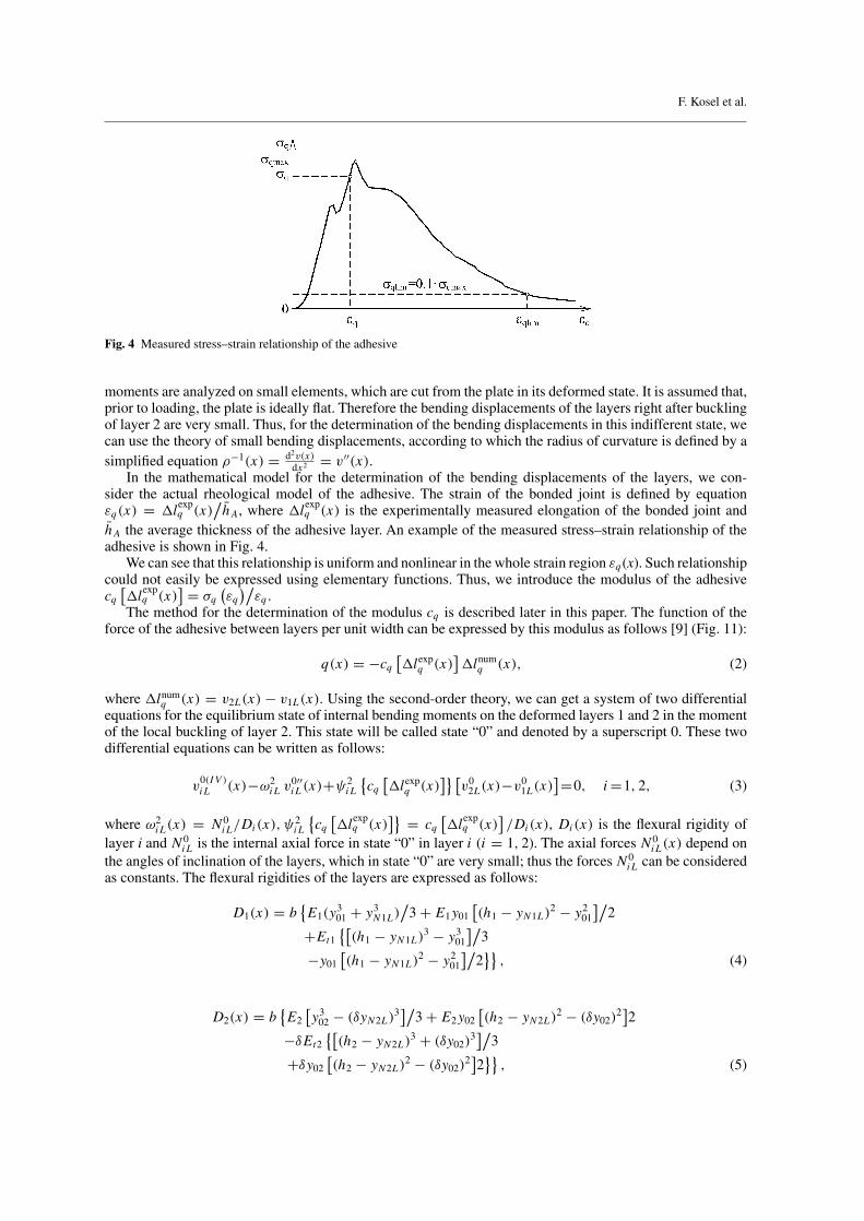
Fig. 4 Measured stress–strain relationship of the adhesive

moments are analyzed on small elements, which are cut from the plate in its deformed state. It is assumed that,prior to loading, the plate is ideally flat. Therefore the bending displacements of the layers right after bucklingof layer 2 are very small. Thus, for the determination of the bending displacements in this indifferent state, wecan use the theory of small bending displacements, according to which the radius of curvature is defined by asimplified equation ρ−1(x) = d2v(x)

dx2 = v′′(x).In the mathematical model for the determination of the bending displacements of the layers, we con-

sider the actual rheological model of the adhesive. The strain of the bonded joint is defined by equationεq(x) = �l

expq (x)

/hA, where �lexp

q (x) is the experimentally measured elongation of the bonded joint andhA the average thickness of the adhesive layer. An example of the measured stress–strain relationship of theadhesive is shown in Fig. 4.

We can see that this relationship is uniform and nonlinear in the whole strain region εq(x). Such relationshipcould not easily be expressed using elementary functions. Thus, we introduce the modulus of the adhesivecq[�l

expq (x)

] = σq(εq)/εq .

The method for the determination of the modulus cq is described later in this paper. The function of theforce of the adhesive between layers per unit width can be expressed by this modulus as follows [9] (Fig. 11):

q(x) = −cq[�lexp

q (x)]�lnum

q (x), (2)

where �lnumq (x) = v2L(x) − v1L(x). Using the second-order theory, we can get a system of two differential

equations for the equilibrium state of internal bending moments on the deformed layers 1 and 2 in the momentof the local buckling of layer 2. This state will be called state “0” and denoted by a superscript 0. These twodifferential equations can be written as follows:

v0(IV )iL (x)−ω2

iL v0′′iL(x)+ψ2

iL

{cq[�lexp

q (x)]} [

v02L(x)−v0

1L(x)]=0, i=1, 2, (3)

where ω2iL(x) = N0

iL/Di(x), ψ2iL

{cq[�l

expq (x)

]} = cq[�l

expq (x)

]/Di(x), Di(x) is the flexural rigidity of

layer i and N0iL is the internal axial force in state “0” in layer i (i = 1, 2). The axial forces N0

iL(x) depend onthe angles of inclination of the layers, which in state “0” are very small; thus the forces N0

iL can be consideredas constants. The flexural rigidities of the layers are expressed as follows:

D1(x) = b{E1(y

301 + y3

N1L)/

3 + E1y01[(h1 − yN1L)

2 − y201

]/2

+Et1{[(h1 − yN1L)

3 − y301

]/3

−y01[(h1 − yN1L)

2 − y201

]/2}}, (4)

D2(x) = b{E2

[y3

02 − (δyN2L)3]/

3 + E2y02[(h2 − yN2L)

2 − (δy02)2]2

−δEt2{[(h2 − yN2L)

3 + (δy02)3]/

3

+δy02[(h2 − yN2L)

2 − (δy02)2]2}}, (5)


where δ = 1 for 0 ≤ |x| < LP/2 and δ = −1 for LP/2 < |x| ≤ L0/2. According to Fig. 2, we can write thefollowing nonhomogeneous boundary conditions:

1. v01L(0) = 0; 2. v0′

1L(0) = 0; 3. v0′2L(0) = 0

4. v01L (L0/2) = v0

2L (L0/2) ; 5. v0′1L (L0/2) = v0′

2L (L0/2)6. M0

1L (L0/2) = D1 (L0/2) v0′′1L (L0/2)

= M0 (1 − b1/L1)−MBL − F0v01L (L0/2)

−N2BL[v0

2L(0)− v01L (L0/2)

]

7. M02L (L0/2)=D2 (L0/2) v0′′

2L (L0/2)=−MBL−N2BL[v0

2L(0)−v02L (L0/2)

]

8. Q01L (L0/2) = D1 (L0/2) v0′′′

1L (L0/2) = − (N2BL − F0) v0′1L (L0/2) .

(6)

Applying the second-order theory, we can accept the following simplified expression for the shear forceQ0

1L (L0/2) in the boundary conditions (6):

Q01L (L0/2) = − (N2BL − F0) sin α0

1L (L0/2) ≈ − (N2BL − F0) v0′1L (L0/2) .

The set of equations (3) is nonlinear. An analytical solution would be very difficult to obtain, thus, we will tryto get a numerical solution. Using the method of finite differences, we divide the length (L0/2) into n = 100intervals of equal length. In this way, considering the boundary conditions (6), we can transform solving ofthe set (3) into solving a system of (2n + 8) nonhomogeneous linear equations and solve it numerically byusing the Gaussian elimination method [10]. The set of nonlinear equation (3) can be solved successively. Inthe first step, we choose cq

[�l

expq (x)

]=0 and determine the deflections v0

iL(x) of the layer i (i = 1, 2) and�lnum

q (x) = v2L(x)−v1L(x). From the diagram of cq(�l

expq

)(Fig. 19), we determine the modulus cq

(�lnum

q

).

The described procedure is repeated until the following condition is fulfilled:∣∣�lnum

q (j)−�lnumq (j − 1)

∣∣ ≤ ε.The chosen accuracy ε = 10−5 mm is reached after eight steps. Thus, we obtain the bending displacementsv0iL(x) of layer i (i = 1, 2) in the domain 0 ≤ |x| ≤ L0/2 in the state “0”.

3.2 The force at which an unstable state in layer 2 occurs and the critical external bending moment

In the described model for the determination of the bending displacements of layers in the moment rightafter local buckling of layer 2, the internal axial force N2BL in layer 2 and the external bending moment M0(Fig. 2) are treated as unknowns. Layer 2 buckles locally in the moment at which the compressive axial forcein the layer reaches the critical value, N cr

2L. Furthermore, it is assumed that layer 2 is bonded to layer 1 withan adhesive whose rigidity is represented by the modulus cq . The bending moment in layer 2 at point C isM0

2L (L0/2) = k v0′2L (L0/2), where k is expressed by the equation: k = 2L1Deq (L0/2) /L0 (L1 − L0). Here,

the flexural rigidity is

Deq(x) = b{T1(x) h1

[h2

1 − 3h1 yNL + 3y2NL

]+ T2(x) h2[h2

2 + 3h1 (h1 + h2)

−3 (2 h1 + h2) yNL + 3 y2NL

]} /3 , (7)

where Ti(x) = Di(x)/Izi , Izi = bh3

i

/12 is the second moment of area of layer i (i = 1, 2), and yNL= yNL( x)

is the distance of the neutral axis from the bottom plane of the plate (Fig. 5).

Fig. 5 Normal stress in the plate due to F0 and M0

F. Kosel et al.

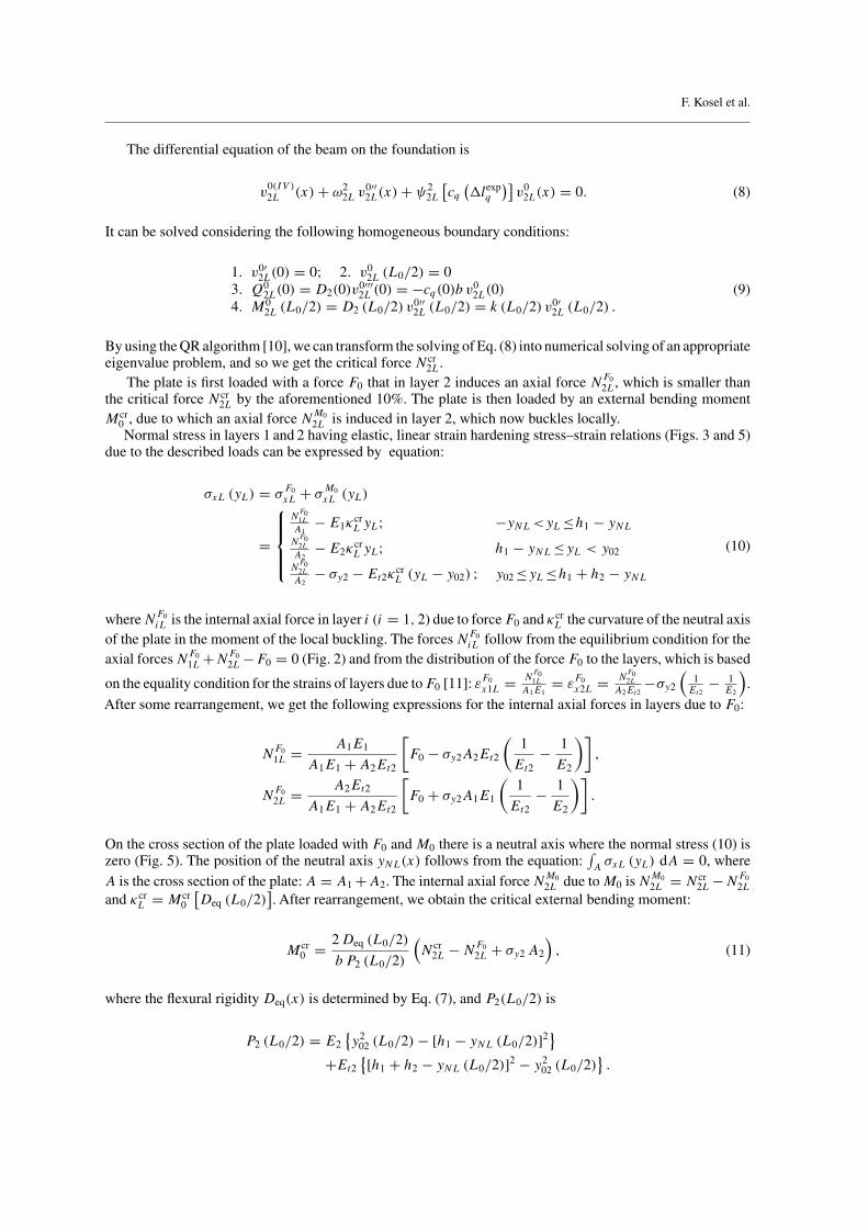
The differential equation of the beam on the foundation is

v0(IV )2L (x)+ ω2

2L v0′′2L(x)+ ψ2

2L

[cq(�lexp

q

)]v0

2L(x) = 0. (8)

It can be solved considering the following homogeneous boundary conditions:

1. v0′2L(0) = 0; 2. v0

2L (L0/2) = 03. Q0

2L(0) = D2(0)v0′′′2L (0) = −cq(0)b v0

2L(0)4. M0

2L (L0/2) = D2 (L0/2) v0′′2L (L0/2) = k (L0/2) v0′

2L (L0/2) .(9)

By using the QR algorithm [10], we can transform the solving of Eq. (8) into numerical solving of an appropriateeigenvalue problem, and so we get the critical force N cr

2L.The plate is first loaded with a force F0 that in layer 2 induces an axial force NF0

2L, which is smaller thanthe critical force N cr

2L by the aforementioned 10%. The plate is then loaded by an external bending momentMcr

0 , due to which an axial force NM02L is induced in layer 2, which now buckles locally.

Normal stress in layers 1 and 2 having elastic, linear strain hardening stress–strain relations (Figs. 3 and 5)due to the described loads can be expressed by equation:

σxL (yL) = σF0xL + σ

M0xL (yL)

=

NF01LA1

− E1κcrL yL; −yNL<yL≤h1 − yNL

NF02LA2

− E2κcrL yL; h1 − yNL≤yL < y02

NF02LA2

− σy2 − Et2κcrL (yL − y02) ; y02 ≤yL≤h1 + h2 − yNL

(10)

whereNF0iL is the internal axial force in layer i (i = 1, 2) due to forceF0 and κcr

L the curvature of the neutral axisof the plate in the moment of the local buckling. The forces NF0

iL follow from the equilibrium condition for theaxial forcesNF0

1L+NF02L−F0 = 0 (Fig. 2) and from the distribution of the force F0 to the layers, which is based

on the equality condition for the strains of layers due toF0 [11]: εF0x1L = N

F01L

A1E1= ε

F0x2L = N

F02L

A2Et2−σy2

(1Et2

− 1E2

).

After some rearrangement, we get the following expressions for the internal axial forces in layers due to F0:

NF01L = A1E1

A1E1 + A2Et2

[F0 − σy2A2Et2

(1

Et2− 1

E2

)],

NF02L = A2Et2

A1E1 + A2Et2

[F0 + σy2A1E1

(1

Et2− 1

E2

)].

On the cross section of the plate loaded with F0 and M0 there is a neutral axis where the normal stress (10) iszero (Fig. 5). The position of the neutral axis yNL(x) follows from the equation:

∫AσxL (yL) dA = 0, where

A is the cross section of the plate:A = A1 +A2. The internal axial forceNM02L due toM0 isNM0

2L = N cr2L−NF0

2Land κcr

L = Mcr0

[Deq (L0/2)

]. After rearrangement, we obtain the critical external bending moment:

Mcr0 = 2Deq (L0/2)

b P2 (L0/2)

(N cr

2L −NF02L + σy2 A2

), (11)

where the flexural rigidity Deq(x) is determined by Eq. (7), and P2(L0/2) is

P2 (L0/2) = E2{y2

02 (L0/2)− [h1 − yNL (L0/2)]2}

+Et2{[h1 + h2 − yNL (L0/2)]

2 − y202 (L0/2)

}.


Fig. 6 Normal stress in layer 1

3.3 Stresses and bending displacement states of the debonded part of the platein the postbuckled state—Phase 2

After the local buckling process of layer 2 has been completed, the plate is in the postbuckled state. In themoment right after layer 2 has locally buckled (state “0”), the plate is loaded with axial force F0 and criticalbending moment Mcr

0 . From the previously derived bending displacement states in state “0”, the curvatures

of layers κ0iL

(Mcr

0 , F0, x) = v0′′

iL(x){1+[v0′

iL(x)]2}3/2 , i=1, 2, the stresses, internal axial forces and internal bending

moments in the layers are obtained.The stress in layer 1 (Fig. 6) due to the axial force and bending moment, considering Eq. (1), is expressed

as follows:

σx1L (y1L) = σF0x1L + σ

M0x1L (y1L)

={

− σy1

y01y1L; −yN1L ≤ y1L ≤ y01

−σy1 − Et1E1

σy1

y01(y1L − y01) ; y01 < y1L ≤ h1 − yN1L

(12)

The depth of the plastified domain of the cross section can be expressed at the point between the elastic andplastic domain of the cross section of layer 1: y01(x) = σy1

/[E1κ

01L(x)

]. The radius of curvature κ−1

1L (x)refers to the neutral axis. Considering Eq. (12), we obtain the internal axial force and bending moment fromequilibrium conditions for the internal axial forces and bending moments:

N01L(x) = −

∫

A1

σx1L (y1L) dA1 (y1L)

= −b{

σy1

(y2

01 − y2N1L

)

(2y01)+ σy1 (h1 − yN1L − y01)

(1 − Et1

E1

)

+Et1κ01L

[(h1 − yN1L)

2 − y201

] /2

}

(13)

M01L(x) = −

∫

A1

σx1 (y1L) y1L dA1 (y1L)

= −b {σy1(y3

01 + y3N1L

)/ (3y01)

+σy1[(h1 − yN1L)

2 − y201

] (1 − Et1

/E1) /

2

+Et1κ01L

[(h1 − yN1L)

3 − y301

] /3}, (14)

where dA1(y1L) = bdy1L. From Fig. 2, we can see that on the bending displacements curve of layer 2 afterlocal buckling an inflection point at |x| = LP/2 exists where the curvature κ0

2L changes its sign. At this pointonly the stress due to the internal axial force N0

2L exists. Hence, we consider two domains of layer 2 in whichwe analyze the stress, internal axial force and bending moment.

F. Kosel et al.

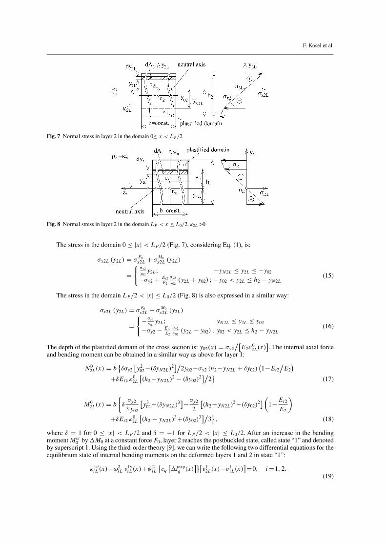
Fig. 7 Normal stress in layer 2 in the domain 0≤ x < LP /2

Fig. 8 Normal stress in layer 2 in the domain LP < x ≤ L0/2, κ2L >0

The stress in the domain 0 ≤ |x| < LP/2 (Fig. 7), considering Eq. (1), is:


M0x2L (y2L)

={σy2

y02y2L; −yN2L ≤ y2L ≤ −y02

−σy2 + Et2E2

σy2

y02(y2L + y02) ; −y02 < y2L ≤ h2 − yN2L

(15)

The stress in the domain LP/2 < |x| ≤ L0/2 (Fig. 8) is also expressed in a similar way:


M0x2L (y2L)

={

− σy2

y02y2L; yN2L ≤ y2L ≤ y02

−σy2 − Et2E2

σy2

y02(y2L − y02) ; y02 < y2L ≤ h2 − yN2L

(16)

The depth of the plastified domain of the cross section is: y02(x) = σy2/[E2κ

02L(x)

]. The internal axial force

and bending moment can be obtained in a similar way as above for layer 1:

N02L(x) = b

{δσy2

[y2

02−(δyN2L)2]/

2y02−σy2 (h2−yN2L + δy02)(1−Et2

/E2)

+δEt2 κ02L

[(h2−yN2L)

2 − (δy02)2]/

2}

(17)

M02L(x) = b

{δσy2

3 y02

[y3

02−(δyN2L)3]− σy2

2

[(h2−yN2L)

2−(δy02)2] (

1−Et2E2

)

+δEt2 κ02L

[(h2 − yN2L)

3+(δy02)3]/

3}, (18)

where δ = 1 for 0 ≤ |x| < LP/2 and δ = −1 for LP/2 < |x| ≤ L0/2. After an increase in the bendingmomentMcr

0 by�M0 at a constant force F0, layer 2 reaches the postbuckled state, called state “1” and denotedby superscript 1. Using the third-order theory [9], we can write the following two differential equations for theequilibrium state of internal bending moments on the deformed layers 1 and 2 in state “1”:

κ1′′iL (x)−ω2

iL v1′′iL(x)+ψ2

iL

{cq[�lexp

q (x)]}[v1

2L(x)−v11L(x)

]=0, i=1, 2.(19)


The curvature κ1iL(x) of layer i in state “1” is:

κ1′′iL (x) =

v1′′iL(x){

1 + [v1′iL(x)

]2}3/2

′′

, i = 1, 2, 0 ≤ x ≤ L0/2. (20)

According to Fig. 2, we can write the following nonhomogeneous boundary conditions:

1. v11L(0)=0; 2. v1′

1L(0)=0; 3. v1′2L(0)=0

4. v11L (L0/2)=v1

2L (L0/2) ; 5. v1′1L (L0/2) = v1′

2L (L0/2)6. M1

1L (L0/2)=D1 (L0/2) v1′′1L (L0/2)

= M0(1 − b1

/L1)−MBL + F0

[v0T L − v1

1L (L0/2)]

−N2BL[v1

2L(0)− v11L (L0/2)

]

7. M12L (L0/2)=D2 (L0/2) v1′′

2L (L0/2)=−MBL−N2BL[v1

2L(0)−v12L (L0/2)

]

8. Q11L (L0/2)=D1 (L0/2) v1′′′

1L (L0/2)=− (N2BL − F0) sin α11L (L0/2) .

(21)

In the boundary condition for M11L (L0/2) in equation (21), we consider the bending deflection v0

T L in thepreceding step of loading, that is, in state “0”. In the jth step of loading, we consider the deflection vj−1

T L in the(j − 1)th step of loading.

Using the method of finite differences, we transform the solving of the set of equations (19), consideringthe boundary conditions (21), into solving a system of (2n + 8) nonhomogeneous nonlinear equations. Wesolve it numerically by using the modified Powell’s algorithm [12]. As the initial bending displacements weuse those which were determined in state “0”: v0

1L(x) and v02L(x). Thus, we obtain the bending displacements

v1iL(x) and curvatures κ1

iL(x) of layer i (i = 1, 2) in the domain 0 ≤ |x| ≤ L0/2 in state “1”. The internal axialforces and bending moments follow from Eqs. (13), (14), (17) and (18) with the replacement of the superscript“0” with “1”. The described procedure is repeated during the entire process of increasing bending momentM0by �M0 at a constant force F0.

3.4 Bonded part of the plate—Phases 1 and 2

If the plate is cut through in the bonded domain in the very vicinity of point C (Fig. 9), the domain C–T canbe treated as a cantilever beam bonded of two layers having certain mechanical properties. We can replace theinfluence of the left part cut off on its right by the external force F0 and the bending moments MCL and MTL.

For the equilibrium state of internal bending moment, we can obtain a differential equation for the deter-mination of the bending displacements of the bonded part:

κ ′′L(x)+ ω2

L

[v′′CL(x)+ v′′

L(x)] = 0, (22)

where κL(x) is the curvature of the bonded part and ω2L = F0

/[Deq (L0/2)

]. The second derivative of κL(x) is

determined by Eq. (20) and the flexural rigidityDeq(x) by Eq. (7). Considering the nonhomogeneous boundary

Fig. 9 Bonded part of the plate

F. Kosel et al.

Fig. 10 Normal stress in the bonded part of the plate

conditions (Fig. 9)

1. vL (L0/2) = vCL; 3. v′L (L1/2) = 0

2. v′L (L0/2) = tan αCL; 4. v′′

L (L0/2) = v′′CL = MCL

/[Deq (L0/2)

] (23)

and by using the method of finite differences, we transform the solving of the differential equation (22) intonumerical solving of a system of (n+ 4) nonlinear equations. This is solved in the way described above withn = 100 intervals. Thus we obtain the bending displacements vL(x) of the bonded part in all states during theentire process of increasing the external loading.

Considering the stress–strain relations (1) of both layers and according to Fig. 10, we can determine thenormal stress in the bonded part due to the loading with the axial force and bending moment:

σxL (yL) =

−σy1 + Et1E1

σy1

y0(y0 + yL) ; −yNL ≤ yL < −y0

σy1

y0yL; −y0 ≤ yL ≤ h1 − yNL

E2E1

σy1

y0yL; h1 − yNL ≤ yL ≤ h1 + h2 − yNL

(24)

From the way of loading and chosen materials of both layers it is shown that plastification first takes place inlayer 1. Therefore, the depth of the plastified domain can be determined in the point between the elastic andplastic domain of the cross section of layer 1: y0(x) = σy1

/[E1κL(x)]. The internal axial force and bending

moment follow from the equilibrium conditions, considering Eq. (24):

NL(x) = −∫

A

σxL (yL) dA (yL)

= −b σy1

{(yNL − y0)+ Et1

E1

1

y0

[y0 (y0 − yNL)− 1

2

(y2

0 − y2NL

)]

− 1

2y0

[(h1 − yNL)

2 − y20

]− E2

E1

h2

2y0[h2 + 2 (h1 − yNL)]

}(25)

ML(x) = −∫

A

σxL (yL) yL dA (yL)

= −b σy1

{1

2

(y2

0 − y2NL

)− Et1

E1

1

y0

[y0

2

(y2

0 − y2N

)+ 1

3

(y3NL − y3

0

)]

− 1

3y0

[(h1 − yNL)

3 + y30

]

−E2

E1

1

3y0

[(h1 + h2 − yN)

3 − (h1 − yNL)3]}

(26)

3.5 Mechanism of growth of the debonded area

In the initial phase of the process, external loads are small and strains in both layers are equal. When theexternal loads increase, the stress and strain in the adhesive increase too. At the moment of local buckling of


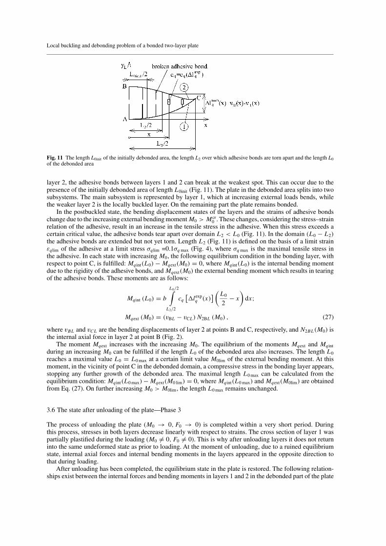
Fig. 11 The length L0init of the initially debonded area, the length L2 over which adhesive bonds are torn apart and the length L0of the debonded area

layer 2, the adhesive bonds between layers 1 and 2 can break at the weakest spot. This can occur due to thepresence of the initially debonded area of length L0init (Fig. 11). The plate in the debonded area splits into twosubsystems. The main subsystem is represented by layer 1, which at increasing external loads bends, whilethe weaker layer 2 is the locally buckled layer. On the remaining part the plate remains bonded.

In the postbuckled state, the bending displacement states of the layers and the strains of adhesive bondschange due to the increasing external bending momentM0 > Mcr

0 . These changes, considering the stress–strainrelation of the adhesive, result in an increase in the tensile stress in the adhesive. When this stress exceeds acertain critical value, the adhesive bonds tear apart over domain L2 < L0 (Fig. 11). In the domain (L0 − L2)the adhesive bonds are extended but not yet torn. Length L2 (Fig. 11) is defined on the basis of a limit strainεqlim of the adhesive at a limit stress σqlim =0.1σq max (Fig. 4), where σq max is the maximal tensile stress inthe adhesive. In each state with increasing M0, the following equilibrium condition in the bonding layer, withrespect to point C, is fulfilled: Mqint(L0)−Mqext(M0) = 0, where Mqint(L0) is the internal bending momentdue to the rigidity of the adhesive bonds, andMqext(M0) the external bending moment which results in tearingof the adhesive bonds. These moments are as follows:

Mqint (L0) = b

L0/2∫

L2/2

cq[�lexp

q (x)] (L0

2− x

)dx;

Mqext (M0) = (vBL − vCL)N2BL (M0) , (27)

where vBL and vCL are the bending displacements of layer 2 at points B and C, respectively, and N2BL(M0) isthe internal axial force in layer 2 at point B (Fig. 2).

The moment Mqext increases with the increasing M0. The equilibrium of the moments Mqext and Mqintduring an increasing M0 can be fulfilled if the length L0 of the debonded area also increases. The length L0reaches a maximal value L0 = L0 max at a certain limit value M0lim of the external bending moment. At thismoment, in the vicinity of point C in the debonded domain, a compressive stress in the bonding layer appears,stopping any further growth of the debonded area. The maximal length L0 max can be calculated from theequilibrium condition:Mqint(L0 max)−Mqext(M0 lim) = 0, whereMqint(L0 max) andMqext(M0lim) are obtainedfrom Eq. (27). On further increasing M0 > M0lim, the length L0 max remains unchanged.

3.6 The state after unloading of the plate—Phase 3

The process of unloading the plate (M0 → 0, F0 → 0) is completed within a very short period. Duringthis process, stresses in both layers decrease linearly with respect to strains. The cross section of layer 1 waspartially plastified during the loading (M0 �= 0, F0 �= 0). This is why after unloading layers it does not returninto the same undeformed state as prior to loading. At the moment of unloading, due to a ruined equilibriumstate, internal axial forces and internal bending moments in the layers appeared in the opposite direction tothat during loading.

After unloading has been completed, the equilibrium state in the plate is restored. The following relation-ships exist between the internal forces and bending moments in layers 1 and 2 in the debonded part of the plate

F. Kosel et al.

Fig. 12 Normal stresses in layer 1 in all three phases of the process

in all three phases of the process, that is, during the process of loading, during the process of unloading and inthe state after unloading:

NiR(x) = NiL(x)+NiU(x), QiR(x) = QiL(x)+QiU(x)MiR(x) = MiL(x)+MiU(x), i = 1, 2, 0 ≤ |x| ≤ L0/2 .

(28)

The bending displacement states of layers 1 and 2 in the debonded part of the plate in all phases of the processmust satisfy the following conditions [13]:

viR(x) = viL(x)+ viU (x), i = 1, 2, 0 ≤ |x| ≤ L0/2, (29)

or in terms of curvatures:

κiR(x) = κiL(x)+ κiU (x), i = 1, 2, 0 ≤ |x| ≤ L0/2. (30)

In layer 1 (Fig. 12), the process of unloading follows a straight line in the σ–ε diagram. The neutral axis duringunloading coincides with the centroid c1 of the cross section and thus the curvature κ1U during unloading is:

κ1U(x) = −εM1Ux1U (x)

η1(x)= −σM1U

x1U (η1)

[E1 η1(x)], (31)

where η1 = η1(x) is the distance from the centroid (Fig. 12).The bending stress σM1U

x1U (η1) during unloading can be obtained by introducing Eq. (31) into Eq. (30)and considering the following relationship between the coordinates η1, y1U and � yN1U (Fig. 12): η1(x) =y1U(x)−�yN1U(x). After some rearrangement, we get:

σM1Ux1U (y1U) = (y1U −�yN1U)

(σy1/y01 − E1 κ1R

). (32)

The stress σN1Ux1U due to the axial force N1U during unloading can be expressed by the force N1U and the cross

section A1. From Fig. 12 we can also see that between the stress σN1Ux1U , the curvature κ1U and the distance�yN1U ,

the following relationship exists: σN1Ux1U = −E1κ1U�yN1U . Introducing Eqs. (31) and (32) and expression for

η1(x) into the mentioned relationship, we get:

σN1Ux1U = N1U

/A1 = const. = −E1 κ1U �yN1U = �yN1U

(σy1

/y01 − E1 κ1R

).

(33)

The stress during the unloading is the sum of Eqs. (32) and (33):

σx1U (y1U) = σN1Ux1U (y1U)+ σ

M1Ux1U (y1U) = y1U

(σy1

/y01 − E1 κ1R

). (34)

The axial force during unloading can be obtained from the equilibrium condition in the cross section of thelayer for internal axial forces:

N1U = −∫

A1

σx1U (y1U) dA1 (y1U) = − b h1�yN1U(σy1

/y01 − E1 κ1R

), (35)


where is dA1(y1U) = bdy1U . The internal bending moment during unloading acts at the centroid and followsfrom the equilibrium condition in the cross section of the layer for bending moments:

M1U = −∫

A1

σx1U (y1U) y1U dA1 (y1U)

= −b h1(σy1

/y01 − E1 κ1R

) (h2

1 + 12�y2N1U

)/12. (36)

By introducing Eqs. (13), (14), (35) and (36) into Eq. (28), we get the resulting internal axial force and bendingmoment in layer 1 in the state after unloading:

N1R = N1L +N1U for 0 ≤ |x| ≤ L0/2

N1R = −b{σy1

2y01

(y2

01 − y2N1L

)+ σy1 (h1 − yN1L − y01)

(1 − Et1

E1

)

+Et1 κ1L

2

[(h1 − yN1L)

2 − y201

]}

− b h1�yN1U

(σy1

y01− E1 κ1R

)

(37)

M1R = M1L +M1U for 0 ≤ |x| ≤ L0/2

M1R = −b{σy1

3y01

(y3

01 + y3N1L

)+ σy1

2

[(h1 − yN1L)

2 − y201

](

1 − Et1

E1

)

+ Et1 κ1L

3

[(h1 − yN1L)

3 − y301

]}

−b h1

12

(σy1

y01− E1 κ1R

) (h2

1 + 12�y2N1U

). (38)

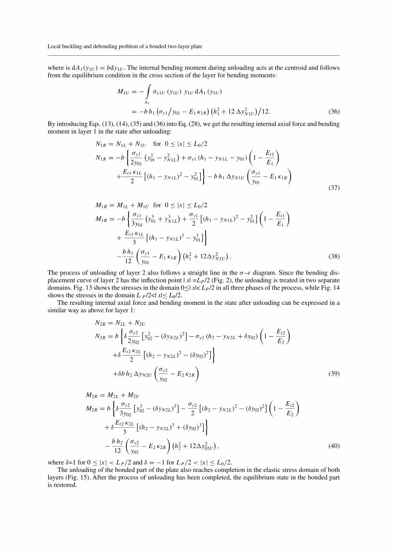
The process of unloading of layer 2 also follows a straight line in the σ–ε diagram. Since the bending dis-placement curve of layer 2 has the inflection point | x| =LP /2 (Fig. 2), the unloading is treated in two separatedomains. Fig. 13 shows the stresses in the domain 0≤| x|< LP /2 in all three phases of the process, while Fig. 14shows the stresses in the domain L P /2<| x|≤ L0/2.

The resulting internal axial force and bending moment in the state after unloading can be expressed in asimilar way as above for layer 1:

N2R = N2L +N2U

N2R = b

{δσy2

2y02

[y2

02 − (δyN2L)2]− σy2 (h2 − yN2L + δy02)

(1 − Et2

E2

)

+δEt2 κ2L

2

[(h2 − yN2L)

2 − (δy02)2]}

+δb h2�yN2U

(σy2

y02− E2 κ2R

)(39)

M2R = M2L +M2U

M2R = b

{δσy2

3y02

[y3

02 − (δyN2L)3]− σy2

2

[(h2 − yN2L)

2 − (δy02)2] (

1 − Et2

E2

)

+ δEt2 κ2L

3

[(h2 − yN2L)

3 + (δy02)3]}

− b h2

12

(σy2

y02− E2 κ2R

) (h2

2 + 12�y202U

), (40)

where δ=1 for 0 ≤ |x| < LP/2 and δ = −1 for LP/2 < |x| ≤ L0/2.The unloading of the bonded part of the plate also reaches completion in the elastic stress domain of both

layers (Fig. 15). After the process of unloading has been completed, the equilibrium state in the bonded partis restored.

F. Kosel et al.

Fig. 13 Normal stresses in layer 2 in the domain 0≤| x|< LP /2 in all three phases of the process

Fig. 14 Normal stresses in layer 2 in the domain LP /2<| x|≤ L0/2 in all three phases of the process

Fig. 15 Normal stresses in the bonded part of the plate in all three phases of the process

The following relationships exist between the internal forces and bending moments in the bonded partduring loading, unloading and in the state after unloading:

NR(x) = NL(x)+NU(x), QR(x) = QL(x)+QU(x)

MR(x) = ML(x)+MU(x), L0/2 ≤ |x| ≤ L1/2 . (41)

The bending displacements and curvatures in all phases of the process must satisfy the following condition [13]:

vR(x) = vL(x)+ vU(x), κR(x) = κL(x)+ κU(x), L0/2 ≤ |x| ≤ L1/2.(42)

The curvature κU during unloading refers to the neutral axis nU during unloading and has the opposite sign tothat during loading. It can be expressed by the coordinate η(x):

κU(x) = −σMU

x1U(η)

E1 η(x). (43)

The bending stress σMU

x1U(η) in layer 1 of the bonded part during unloading can be obtained by introduc-ing Eq. (43) into Eq. (42) and considering the relationship between the coordinates η and yU (Fig. 15):�yNU(x) = η(x)−yU(x). We also consider the relationship between the bending stresses in the layers during


unloading: σMU

x2U/σMU

x1U = E2/E1. After rearrangement, we get:

σMU

x1U (yU) = (yU +�yNU)(σy1/y01 − E1 κR

) ;σMU

x2U (yU) = E2/E1σMU

x1U (yU) (44)

The stresses in the layers due to the axial force during unloading follow by considering the relations: σNUx1U =NU

/A1 = −MU �yNU

/Iz1 = constant, and σNUx2U

/σNUx1U = E2

/E1:

σNUx1U (yU) = −�yNU

(σy1

/y01 − E1 κR

) ;σNUx2U (yU) = −E2

/E1σ

NUx1U (yU) . (45)

The normal stress in the bonded part during unloading is the sum of Eqs. (44) and (45):

σxU (yU) = yU

(σy1

y0− E1 κR

){1; −yNU ≤ yU ≤ h1 − yNUE2/E1; h1 − yNU ≤ yU ≤ h1 + h2 − yNU

(46)

The internal axial force and bending moment in the bonded part during unloading can be obtained from theequilibrium condition for the axial forces and bending moments:

NU = −∫

A

σxU (yU) dA (yU)

= b [E1 h1 (h1 − 2yNU)+ E2 (2 h1 + h2 − 2yNU)]

× [κR − σy1

/(E1 y0)

] /2 (47)

MU = −∫

A

σxU (yU) yU dA (yU)

= b

2

{E2

E1

[(h1 + h2 − yNU)

3 − (h1 − yNU)3]+ (h1 − yNU)

3 − y3NU

}

×(E1 κR − σy1

y0

), (48)

where dA(yU) = bdyU . The resulting internal axial force and bending moment after unloading follow byintroducing Eqs. (25), (26), (47) and (48) into Eq. (41):

NR = NL +NU for L0/2 ≤ |x| ≤ L1/2

NR = −b σy1

{(yNL − y0)+ Et1

E1

1

y0

[y0 (y0 − yNL)− 1

2

(y2

0 − y2NL

)]

− 1

2 y0

[(h1 − yNL)

2 − y20

]− E2

E1

h2

2y0[h2 + 2 (h1 − yNL)]

}

+b2

[E1h1 (h1 − 2yNU)+ E2 (2h1 + h2 − 2yNU)]

(κR − σy1

E1 y0

)(49)

MR = ML(x)+MU(x) for L0/2 ≤ |x| ≤ L1/2

MR = −b σy1

{1

2

(y2

0 − y2NL

)− Et1

E1

1

y0

[y0

2

(y2

0 − y2NU

)+ 1

3

(y3NL − y3

0

)]

− 1

3y0

[(h1 − yNL)

3 + y30

]− E2

E1

1

3y0

[(h1 + h2 − yN)

3 − (h1 − yNL)3]}

+b2

{E2

E1

[(h1 + h2 − yNU)

3 − (h1 − yNU)3]+ (h1 − yNU)

3 − y3NU

}

×(E1 κR − σy1

y0

). (50)

F. Kosel et al.

4 Experimental work

For experimental evaluation of the mathematical model, we chose a bonded two-layer plate-strip. The layersare made of isotropic materials, while the bonding material is Neoprene adhesive having a certain rheolog-ical model. Experimental work was performed using a Zwick Z050 electronic measurement device (EMD)equipped with Multisens extensometers, nominal force 50 kN, crosshead travel resolution of 0.5 µm and mea-surement range error 0.5% from 1/50 of the nominal force. The EMD makes it possible to load test pieces ina combined way with tensile and compressive axial forces. In our experimental work, we first determined themechanical properties of the chosen materials of the layers and adhesive, and then experimentally verified themathematical model.

4.1 Mechanical properties of chosen materials

According to the standard [14], tensile tests were performed in order to measure the mechanical propertiesof materials of the plate-strip layers. For the thicker layer, we chose Peral AlMg3, Impol Slovenska Bistrica,Slovenia. For the weaker layer, we chose cold-reduced grain-oriented transformer steel Unisil-M 103-27P,Orb Electrical Steel Ltd., Newport, South Wales, UK. The selection of the mentioned materials was based onthe observations during tensile tests, which showed that the stress–strain relationships of both materials wereelastic, linear and strain hardening (Fig. 16).

The following mechanical properties in the tensile stress domain were determined: Young’s modulus E inthe elastic domain, yield stress σy , strain εy at the yield stress and tangent modulus Et in the plastic domain,see Table 1. We estimate that the measured mechanical properties of both materials can also be accepted in thecompressive stress domain.

For bonding the layers, Neoprene adhesive Neostik SK-101, Belinka Kemostik, Slovenia, was chosen.According to the standard [15], the stress–strain relationship of the adhesive was measured on the series of 25test pieces bonded from steel and Peral, see Fig.17.

Test pieces were loaded with the increasing tensile force F. The criterion for stopping the test was a pre-scribed limit elongation of the bonded joint �lexp

q lim=3 mm at which adhesive bonds were to be torn apart. Themeasured stress–strain relationships are shown in Fig.19.

Using the definition cq[�l

expq (x)

] = σq(εq)/εq , we tabulated the average modulus of the adhesive

cq[�l

expq (x)

]with respect to the experimentally measured elongation�lexp

q (x) (Fig.19 right). The strain of thebonded joint is defined by equation εq(x) = �l

expq (x)

/hA, where hA=0.077 mm is the average thickness of the

adhesive layer. The modulus c q in the singular point �lexpq = 0 was calculated by interpolating the tabulated

values. The mechanical properties of the materials of the layers and the average modulus cq were used asinputs to compute the bending displacements of layers.

Fig. 16 Measured stress–strain relations for Peral AlMg3 (left) and Unisil-M 103-27P (right)

Table 1 Average values of mechanical properties of the materials of layers 1 and 2

Material E (N/mm2 ) σy (N/mm2 ) εy Et (N/mm2 )

Peral AlMg3 0.656×105 188.12 4.37×10−3 0.62×104

Unisil-M 103-27P steel 2.048×105 337.33 3.6×10−3 1×104


Fig. 17 Standard test piece for determination of stress–strain relationship of the adhesive [15]

Fig. 18 Principle of compressive-bending experiment

4.2 Experimental verification of the mathematical model

Compressive-bending experiments were performed in order to see how the presented mathematical modelsuited the real conditions. We chose a rigidly fixed plate-strip of width b = 10 mm. The average length oftest pieces was L1= 88.882 mm (Fig.18). The thickness of the layer made of Peral AlMg3 was h1=2 mm andthe thickness of the weaker layer made of Unisil-M 103-27P steel was h2=0.27 mm. A symmetrical initialdebonding was caused over a length L0init =15 mm (Fig.18) by inserting a d=0.19 mm thick wire into the plate(Fig.21).

Due to the vertical orientation of the workplace, it would be very difficult to exert the bending load using acouple of bending moments in the way proposed in the mathematical model. A bending load with a couple ofshear forces F exp

g was applied to the test pieces, which was made possible by a specially designed device thatwas mounted onto the EMD. The method of determination of the forces F exp

g and distance a is explained inFig.20. In case a, the beam is loaded with bending moment M0, while in case b with a couple of forces F exp

g .From the diagrams of bending moments in Fig.20, we can see that the described ways of bending loads arenot comparable with each other.

To obtain correct experimental results in the region of maximal length of debonded area the following threeconditions must be fulfilled:

1. The distance bM between the external moments M0 must be much larger than the maximal length of thedebonded area L0 max of the beam;

2. The maximal bending displacements vD of the beam at point D in cases a and b must be equal;

F. Kosel et al.

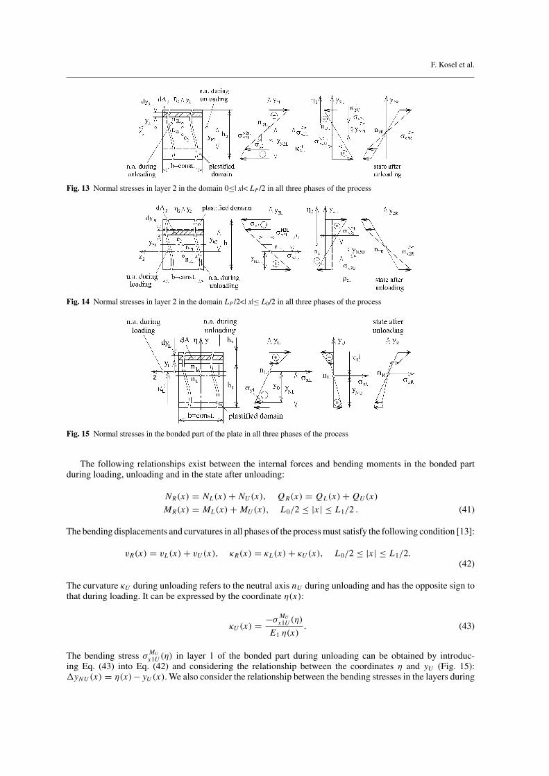
Fig. 19 Measured stress–strain relationships (left) and average modulus cq of the chosen adhesive with respect to elongation�l

expq (right)

Fig. 20 Method of determination of the shear force F expg

3. The maximal internal bending moment at the same point D in cases a and b must be equal. The force F expg

and distance a are as follows:

F expg = 2M0

b1

a21

; a =(3 bM − L1

)

2. (51)

The internal bending moments over the length a > L0 max in both cases a and b are constant and equal:Ma

max = Mbmax = Mmax. The differences between the bending displacements and relative differences between

internal bending moments at points G, E and D in both cases a and b are as follows:

�vG = vaG − vb

G = −3.867M0/(E Iz);

(Ma

G −MbG

)/Mmax = −0.1711

�vE = vaE − vb

E = 1.294 · 10−3M0/(E Iz);

(Ma

E −MbE

)/Mmax = 0

�vD = vaD − vb

D = 0; (Ma

D −MbD

)/Mmax = 0,

(52)

where Iz = bh3/

12 is the second moment of area, b is the width, h is the thickness of the beam, E is theYoung’smodulus, va

i and vbi are the bending displacements at point i, i = G, E, D in case a and b, respectively. Before


Fig. 21 Method of measurement of the external height hZ and length L0 of the debonded area

loading, a wire of diameter d was inserted between the layers on the initially debonded area of length L0init(Fig. 21). The diameter d was equal to the previously calculated initial internal height hN init of the debondedarea right after local buckling (state “0”).

Using a couple of weightsF expg acting on the distance a, the bending load was applied to the test pieces. The

plate-strip was then loaded by increasing the compressive axial forceF exp0 . After the axial force had reached the

critical value F exp0 = F

exp01 , the weaker layer entered the postbuckled state (state “1”). Bending displacements

of the layers exceeded the initial value d = hN init=0.19 mm. We measured the compressive axial forces F exp01

in the mentioned state “1”. The axial force F0 was further increasing at a constant shear force F expg until it

reached the prescribed value F exp02 = −685 N (state “2”). We measured the external height hexp

Z2 and lengthL

exp02 of the debonded area. The force F0 was further increasing at a constant force F exp

g until it reached theprescribed maximal value F exp

03 = Fexp0 max (Fig.22).

In this state, called state “3”, we measured the external height hexpZ3 and lengthLexp

03 . As the criterion for stop-ping the loading, we chose the axial compressive forceF exp

0 max that had previously been numerically determined.In the state after unloading (state “4”), we measured the external height hexp

Z4 and length Lexp04 .

The experiments were performed using 17 test pieces. Based on the measured results, we calculated theaverage values of the length L 1, critical force F exp

01 for local buckling, external height hexpZ and length L

exp0 of

the debonded area, see Table 2.

Fig. 22 State “3” at maximal axial force F exp0 max at a constant shear force F exp

g

F. Kosel et al.

Table 2 Average values of the measured results of compressive-bending experiments

State “0” State “1” State “2” State “3” State “4”

L 1 (mm) Fexp01 (N) h

expZ2 (mm) L

exp02 (mm) h

expZ3 (mm) L

exp03 (mm) h

expZ4 (mm)

88.882 −438.824 2.793 17.059 3.424 20.353 2.715

5 Numerical example

Based on the presented mathematical model a computer program was developed. It enables the determinationof the critical force Nnum

2Lcr and critical external moment Mnum0cr at which the weaker layer buckles locally, the

computation of the displacement states of the layers in the moment after local buckling, during increasingexternal loading and in the state after unloading. A numerical example was set up to see how the physicalmodel corresponded to the real conditions. A rigidly fixed plate-strip of width b = 10 mm, thickness of layer 1,h1=2 mm, and thickness of layer 2, h2=0.27 mm, was chosen. Other dimensions were as shown in Fig.18. Theaverage values of the measured mechanical properties of the layers (Table 1), the modulus of the adhesivecq(�l

expq

)and the length of L0init = 15 mm over which the layers were initially debonded were considered.

Based on a chosen distance bM and length L1, the distance a=45.559 mm (Fig.20) was calculated.The loading model was chosen so that the axial force F0 performed 90% of the compressive force for

local buckling of layer 2 while the remaining part was contributed by the bending moment M0. This is inaccordance with the assumption made in the mathematical model. In the moment of local buckling of layer 2the following values were computed: critical force for local buckling: Nnum

2Lcr = −588.04 N; critical axialforce: F num

0cr = Nnum2Lcr/0.9 = −653.38 N; critical bending moment:Mnum

0cr =304.14 N mm; the necessary weight:F numgcr =24.525 N; internal and external height of debonded area: hN init=0.19 mm and hnum

Z1 = 1.325 mm; initiallength of debonded area: L0init =15 mm.

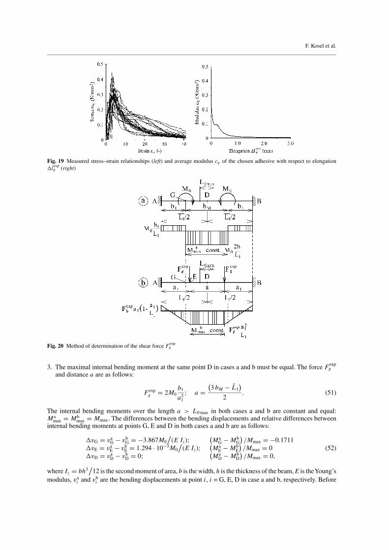
The bending displacements v(x) in the following states of the loading process and in the state after unloadingwere computed, see Fig.23:

– State “1”: Loading with F exp01 = F num

0cr = −653.38 N and F expg = 24.525 N.

– State “2”: Loading with F exp02 = −685 N at a constant value F exp

g = 24.525 N.– State “3”: Loading with F exp

03 = −1433 N at a constant value F expg = 24.525 N.

– State “4”: State after unloading: F exp04 = 0, F exp

g = 0.

From Fig. 23, we can see that the bending displacements increase with increasing axial force F exp0 at a constant

weight F expg . The bending displacements of the bonded part of the plate-strip during increasing F exp

0 (states“1”, “2” and “3”) were determined with an assumed rigid support of the plate-strip at point T, Fig. 2. Afterunloading, i.e. in state “4”, the plate-strip flattens. Due to stresses in the elasto-plastic domain in state “3”, thetangent to the bonded part of the plate-strip at the same point T is no longer parallel to the x-axis, Fig. 23.

Figure 24 presents the length Lnum0 of the debonded area with respect to the bending moment Mnum

0 at aconstant force F exp

03 =−1433 N. The length of the debonded area suddenly increases from L0init =15.0 mm toLnum

0 =16.6 mm at a constant bending moment Mnum0cr =304.14 N mm. This is a consequence of using the sec-

ond-order theory. The lengthL0 then increases with increasing bending moment and reaches its maximal valueLnum

0 max=20.6 mm at the maximal bending momentMnum0 max=404.54 N mm. After unloading of the plate-strip, the

length Lnum0 max remains unchanged.

6 Discussion

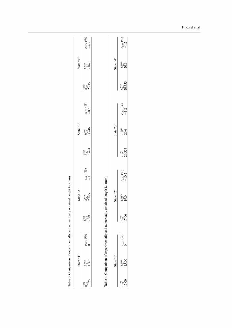
The physical adequacy of the presented mathematical model was evaluated by comparing the numerically andexperimentally obtained results for the external height hZ and lengthL0 of the debonded area. The experimen-tally obtained results in the three states of loading and in the state after unloading were compared by determiningrelative differences with respect to numerically obtained values. Table 3 shows the relative differences ehZibetween the experimentally and numerically obtained results for external height hZ , where i = 1, 2, 3, 4 is thenumber of the state. Table 4 shows the relative differences eL0i between the experimentally and numericallyobtained results for the length L0.

From Table 3, we can see that the maximal relative difference in the external height hZ occurs in state “3”.The relative difference ehZ1 in state “2” is −1.1% and in state “4” is −4.5%, whereas the relative differences


Fig. 23 Bending displacement states of plate-strip in the four states of the process

Fig. 24 Debonded length Lnum0 with respect to the external bending moment Mnum

0

eL0 in states “3” and “4” are the same, i.e. −1.2% (Table 4). These tables show very good agreement betweenthe results obtained in both ways. This is, in our opinion, thanks to the use of the third-order theory in thedevelopment of the mathematical model for the determination of the displacement states of the plate. In thenumerical example, the measured mechanical properties of the chosen materials of layers and adhesive wereconsidered.

All experimentally obtained results are slightly below the numerically obtained ones, which shows thepresence of certain nonidealities. We estimate that the existing differences between the results obtained in bothways can be explained by the assumptions made in the mathematical model, which were the following:

1. The plate was taken to be ideally flat prior to loading.2. In the numerical model, average mechanical properties of materials were considered. During measurement

of mechanical properties of the adhesive a certain scatter of results was observed, which is shown in thedescription of the experimental work.

3. In the mathematical model, the bending load was considered to be performed by a couple of bendingmoments while in the experiments, the bending load was performed by a couple of shear forces.

7 Conclusions

The problem of local buckling of the weaker layer of a two-layer plate loaded with external compressive forceand bending moment is treated. The conditions for the growth of the debonded area in the plate have beenstudied. On the basis of the experiments it can be concluded that the axial force should be slightly lower thanthe buckling force of the weaker layer. Instability and the local buckling process can appear when an additionalbending moment is applied to the plate. The numerical model also confirms this. To see how the presentedmathematical model suited the real conditions, a numerical example has been set up in which experimentallyobtained results were considered.

F. Kosel et al.

Tabl

e3

Com

pari

son

ofex

peri

men

tally

and

num

eric

ally

obta

ined

heig

hth Z

(mm

)

Stat

e“1

”St

ate

“2”

Stat

e“3

”St

ate

“4”

hex

pZ

1h

num

Z1

e hZ

1(%

)h

exp

Z2

hnu

mZ

2e hZ

2(%

)h

exp

Z3

hnu

mZ

3e hZ

3(%

)h

exp

Z4

hnu

mZ

4e hZ

4(%

)1.

325

1.32

50

2.79

32.

825

−1.1

3.42

43.

746

−8.6

2.71

52.

843

−4.5

Tabl

e4

Com

pari

son

ofex

peri

men

tally

and

num

eric

ally

obta

ined

leng

thL

0(m

m)

Stat

e“1

”St

ate

“2”

Stat

e“3

”St

ate

“4”

Lex

p01

Lnu

m01

e L01

(%)

Lex

p02

Lnu

m02

e L02

(%)

Lex

p03

Lnu

m03

e L03

(%)

Lex

p04

Lnu

m04

e L04

(%)

15.0

015

.00

017

.06

19.0

−10.

220

.353

20.6

−1.2

20.3

5320

.6−1

.2


The main subsystem bends due to the proposed external loads, while the remaining subsystem buckleslocally into a shape for which a minimal potential energy is needed. This shape is symmetric with respect tothe symmetric axis of the debonded area. Both subsystems remain bonded over a certain domain. From thegraphs it is shown that the length of the debonded area increases with increasing bending moment at a constantaxial force up to a certain limit value.

The physical adequacy of the mathematical model is evaluated by a comparison of experimentally andnumerically obtained results for the external height and length of the debonded area. The mentioned resultswere compared in the three states of loading process and in the unloaded state by determining the relativedifferences with respect to numerically obtained values. The maximum difference between the results for thelength of the debonded area is −10.2%. The maximum difference for the external height of the debonded areais −8.6%. From these values it can be concluded that results obtained from the two methods are in sufficientagreement.

References

1. Whitcomb, J.D.: Mechanics of instability-related delamination growth. In: Garbo, S.P. (ed.) Composite materials: testingand design, vol 9. ASTM STP 1059. American Society for Testing and Materials, Philadelphia pp. 215–230 (1990)

2. Kardomateas, G.A.: The initial post-buckling and growth behavior of internal delaminations in composite plates. TransASME J Appl Mech 60, 903–910 (1993)

3. Simitses, G.J., Sallam, S., Yin, W.L.: Effect of delamination on axially loaded homogeneous laminated plates. AIAA J 23,1437–1444 (1985)

4. Chai, H.: Three-dimensional analysis of thin film debonding. Int J Fracture 46, 237–256 (1990)5. Whitcomb, J.D.: Finite element analysis of instability related delamination growth. J Comp Mat 15, 403–426 (1981)6. Bruno, D., Grimaldi,A.: Delamination failure of layered composite plates loaded in compression. Int J Sol Struct 26, 313–330

(1990)7. Kosel, F., Kuselj, B., Batista, M.: Delamination of two-layer plate-strip. In: Proceedings of the third international conference

design to manufacture in modern industry, 8–9 September. Portoroz (1997)8. Kuselj, B., Kosel, F.: The growth of debonded area in a bonded two-layer plate-strip. Zangew Math Mech 81(Suppl 2),

313–314 (2001)9. Timoshenko, S.P., Gere, J.M.: Theory of elastic stability, 2nd edn. McGraw-Hill, New York (1961)

10. Gerald, C.F., Wheatley, P.O.: Applied numerical analysis, 6th edn. Addison Wesley/Longman, Reading/London (1999)11. Gere, J.M.: Mechanics of materials, 5th edn. Brooks/Cole, Pacific Grove (2001)12. IMSL.: Fortran subroutines for mathematical applications, Visual Numerics (1997)13. Kosel, F., Borstnik, I.: Bending of the beams of constant cross-section in the elasto-plastic domain. J Mech Eng 9–10 205–208

(1979)14. DIN EN 10002.: Metallic materials; tensile testing; Part 1: method of testing (at ambient temperature). German Version EN

10002–1: 1990 + AC1:1990 (1990)15. ASTM D 897-95a.: Standard test method for tensile properties of bonded joints. American Society for Testing and Materials,

Philadelphia (1995)

local buckling and debonding problem of a bonded...

Documents