Local Group See S&G ch 4•  Our galactic neighborhood consists

of one more 'giant' spiral (M31, Andromeda), a smaller spiral M33 and lots of (>35 galaxies), most of which are dwarf ellipticals and irregulars with low mass; most are satellites of MW, M31 or M33

•  The gravitational interaction between these systems is complex but the local group is apparently bound.

•  Major advantages–  close and bright- all nearby

enough that individual stars can be well measured as well as HI, H2, IR, x-ray sources and even γ-rays

–  wider sample of universe than MW (e.g. range of metallicities, star formation rate etc etc) to be studied in detail

– allows study of dark matter on larger scales and first glimpse at galaxy formation– calibration of Cepheid distance scale

MBW fig 2.31

ARA&A1999, V 9, pp 273-318 The local group of galaxies S. van den BerghStar formation histories in local group dwarf galaxies Skillman, Evan D.New Astronomy Reviews, v. 49, iss. 7-9 p. 453-460.

1

https://sciencesprings.wordpress.com/tag/milky-way/Local Group. Andrew Z. Colvin 3 March 2011

2

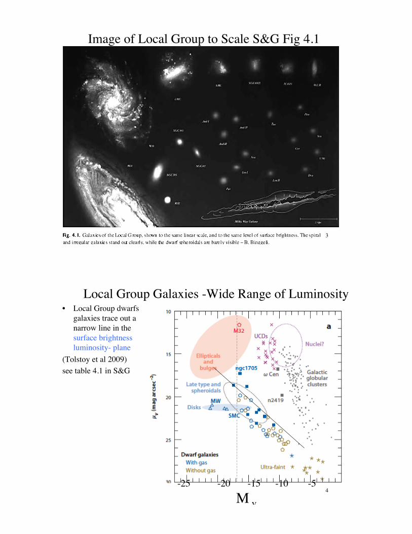
Image of Local Group to Scale S&G Fig 4.1

3

Local Group Galaxies -Wide Range of Luminosity •  Local Group dwarfs

galaxies trace out a narrow line in the surface brightness luminosity- plane

(Tolstoy et al 2009)see table 4.1 in S&G

-25 -20 -15 -10 -5M v

4

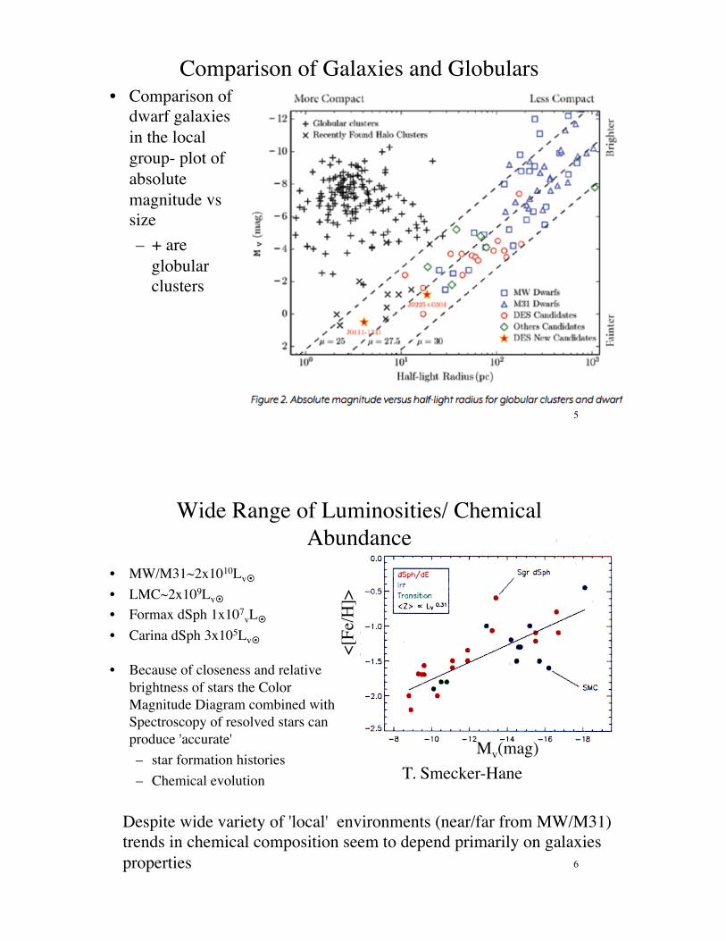
Comparison of Galaxies and Globulars•  Comparison of

dwarf galaxies in the local group- plot of absolute magnitude vs size –  + are

globular clusters

5

•  MW/M31~2x1010Lv¤

•  LMC~2x109Lv¤

•  Formax dSph 1x107vL¤

•  Carina dSph 3x105Lv¤

•  Because of closeness and relative brightness of stars the Color Magnitude Diagram combined with Spectroscopy of resolved stars can produce 'accurate'–  star formation histories–  Chemical evolution T. Smecker-Hane

Mv(mag)

<[Fe

/H]>

Despite wide variety of 'local' environments (near/far from MW/M31)trends in chemical composition seem to depend primarily on galaxiesproperties 6

Wide Range of Luminosities/ Chemical Abundance

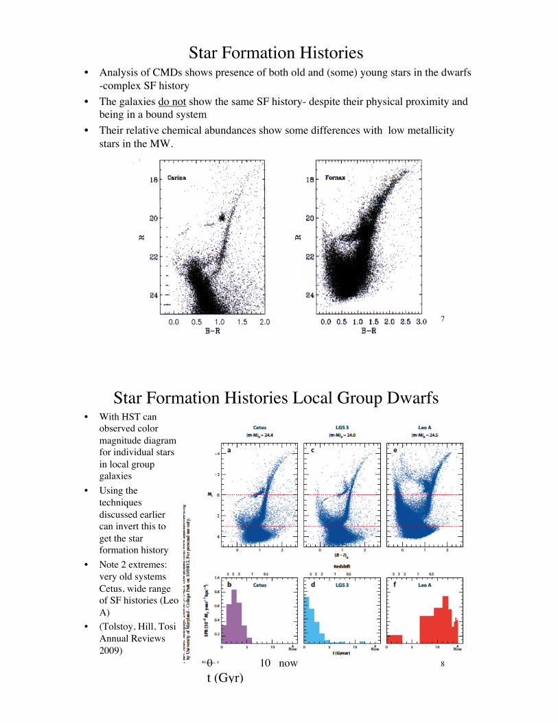
Star Formation Histories •  Analysis of CMDs shows presence of both old and (some) young stars in the dwarfs

-complex SF history•  The galaxies do not show the same SF history- despite their physical proximity and

being in a bound system •  Their relative chemical abundances show some differences with low metallicity

stars in the MW.

7

Star Formation Histories Local Group Dwarfs •  With HST can

observed color magnitude diagram for individual stars in local group galaxies

•  Using the techniques discussed earlier can invert this to get the star formation history

•  Note 2 extremes: very old systems Cetus, wide range of SF histories (Leo A)

•  (Tolstoy, Hill, Tosi Annual Reviews 2009)

0 10 nowt (Gyr)

8

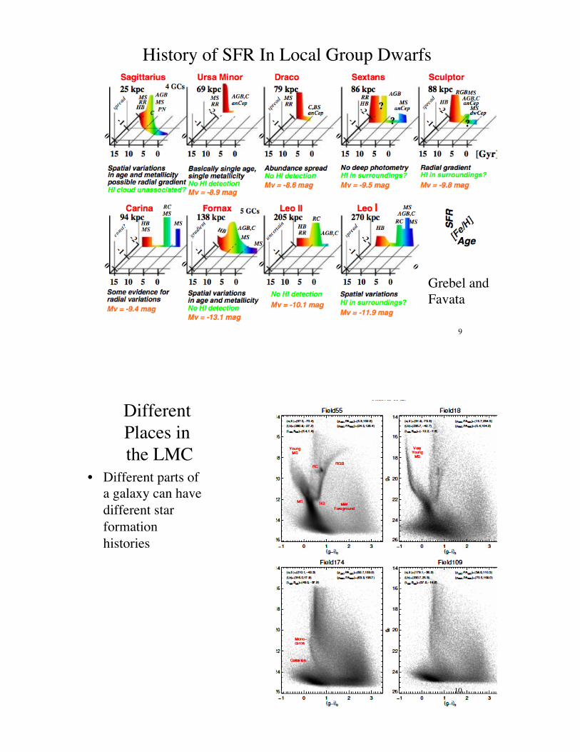
History of SFR In Local Group Dwarfs

Grebel andFavata

9

Different Places in the LMC

•  Different parts of a galaxy can have different star formation histories

10

Abundances in Local Group Dwarfs

•  Clear difference in metal generation compared to MW–  Fe from type I SN–  "α" from type II

•  "α" elements is O,Ne,Mg,Ar,Si,S,

Hill 2008

Sculptor stars in red, MWstars in black

11

Metallicities In LG Dwarfs Vs MW•  Overall metallicity of LG dwarfs is low :patterns but different to stars in MW (black dots- Tolstoy et al 2009)-

•  How to reconcile their low observed metallicity with the fairly high SFR of the most metal-poor systems many of which are actively star-forming

•  best answer metal-rich gas outflows, e.g. galactic winds, triggered by supernova explosions in systems with shallow potential wells, efficiently remove the metal-enriched gas from the system.

•  In Local Group wind models be well constrained by chemical abundance observations (later in lecture).

12

13

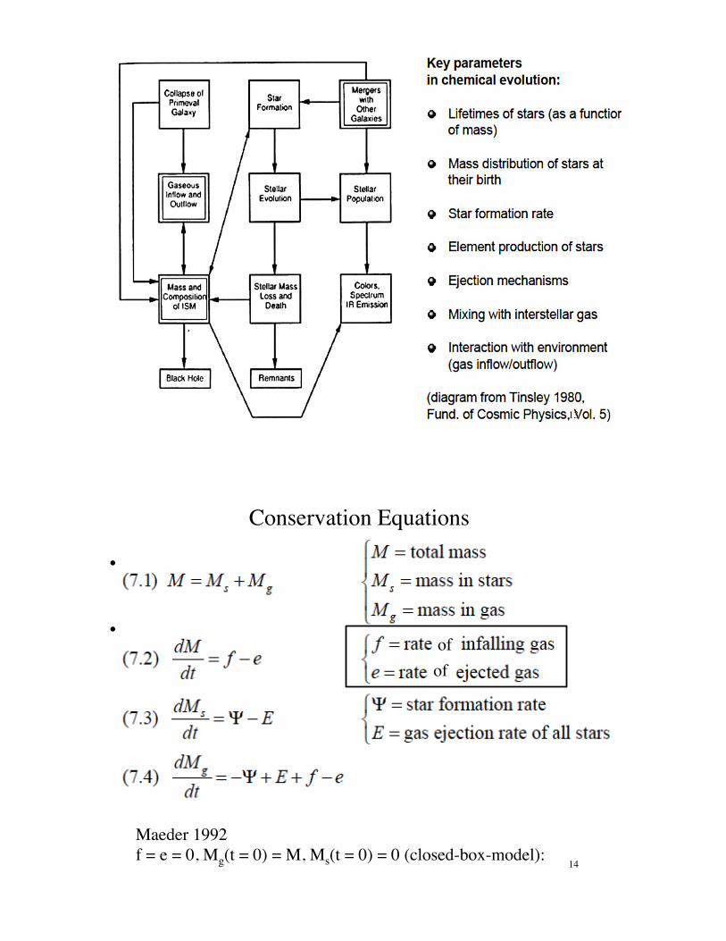
Conservation Equations

•  If we assume that the yield y is independent of time and metallicity ( Z) then

•  Z(t)= Z(0)-y ln Mg(t)/Mg(0)= Z(0)=yln µ

14

Maeder 1992f = e = 0, Mg(t = 0) = M, Ms(t = 0) = 0 (closed-box-model):

ofof

Closed Box Approximation-Tinsley 1980, Fund. Of Cosmic

Physics, 5, 287-388 Read S&G 4.3•  To get a feel for how chemical evolution and SF are related (S+G eqs

4.13-4.17)-

•  at time t, mass ΔMtotal of stars formed, after the massive stars die left with ΔMlow mass which live 'forever'

•  massive stars inject into ISM a mass pΔMtotal of heavy elements (p depends on the IMF and the yield of SN- normalized to total mass of stars).

•  Assumptions: galaxies gas is well mixed, no infall or outflow, high mass stars return metals to ISM faster than time to form new stars)

15

Formation of Elements ala S&G •  Mg(t) the mass of gas in the

galaxy at time t •  M*(t) the mass in low-mass

stars and the white dwarfs, neutron stars and black the matter in these objects remains locked within them throughout the galaxy’s lifetime)

•  Mh(t) is the total mass of elements heavier than helium in the gas;

•  The metal abundance in the gas is then Z(t) =Mh(t)/Mg(t).

16

When the massive stars end their lives, they leave behind a mass ΔM*(t) of low-mass stars and remnants, and return gas to the interstellar medium which includes a mass pΔM*(t) of heavy elements.

The yield is p

So The mass Mh(t) of heavy elements in the interstellar gas changes as the metals produced by massive stars are returned to the gas phase

•  while a mass Z ΔM*(t) of these elements is locked into low-mass stars and remnants.

•  Taking all these terms •  We have•  ΔMh(t)��ΔM*(t) ���ΔM*(t)��������ΔM*(t)

As the stars evolve the metallicity of the gas increases by ΔZ=(Mh(t)/M(t)g)=pΔM*(t)-Z([ΔM*(t)+ΔMg(t)]/Mg(t) eq 4.14Closed box approximation- no gas enters or leaves the system sosum of mass remains constant e.g. ΔM*(t)+ΔMg(t)= 0 (e.g. sum of changes in gas and stellar mass balance)

Integrate eq. 4.14 to get Z(t)=Z(t=0)+pln[Mg(t=0)/Mg(t)] 17

•  Metallicity grows with time as stars form and gas is used up

•  The mass of stars formed before time t is Mg(0)-Mg(t)•  These stars have a metallicity <Z(t) and so •  M*(<Z))=Mg(0)[(1-exp[Z-Z(0)/p)] eq 4.16

•  The mass M*(<Z) of slowly evolving stars that have abundances below the given level Z depends only on the quantity of gas remaining in the galaxy when its metal abundance has reached that value.

•  Once all the gas is gone, this model predicts that the mass of stars with metallicity between Z and Z + Z should be

•  [�*����/dZ] Δ���������������������� ����Δ�� 18

Closed Box- continued •  Net change in metal content of gas•  dMh=p dMstar - Z dMstar=(p- Z) dMstar

•  Change in Z since dMg= -dMstar and Z=Mh/Mg then•  dZ=dMh/Mg -Mh dMg/M2

g =(p- Z) dMstar/Mg +(Mh/Mg)(dMstar/Mg ) =pdMstar /Mg

•  d Z/dt=-p(dMg/dt) Mg

•  If we assume that the yield y is independent of time and metallicity (Z) then

•  Z(t)= Z(0)-p ln Mg(t)/Mg(0) metallicity of gas grows with time logarithmically 4.15

19

Closed Box- continued •  metallicity of gas grows with time logarithmically mass of stars that have a metallicity less than Z(t) is Mstar[< Z(t)]=Mstar(t)=Mg(0)-Mg(t) or Mstar[< Z(t)]=Mg(0)*[1-exp(( Z(t)- Z(0))/p]

when all the gas is gone, mass of stars with metallicity Z, Z+d Z is Mstar[ Z] α exp(( Z(t)- Z(0))/p) d Z- we use this to derive the yield from

data Z(today)~ Z(0-pln[Mg(today)/Mg(0)]; Z(today)~0.7 Zsun

since initial mass of gas was sum of gas today and stars today Mg(0)=Mg(today)+Ms(today) with for MW Mg(today)~10M¤/pc2

Mstars(today)~40M¤/pc2

get p=0.43 Zsun go to pg 180 in text to see sensitivity to average metallicity of stars 20

Closed Box- Problems

21

•  Problem is that closed box connects todays gas and stars yet have systems like globulars with no gas and more or less uniform abundance.

•  Also need to tweak yields and/or assumptions to get good fits to different systems like local group dwarfs.

•  'G dwarf' problem in MW (S+G pg 180-181) nearly half of all stars in the local disk should have less than a quarter of the Sun’s metal content. BUT less than 25% have such low abundances

•  Go to more complex models - leaky box (e.g inflow/outflow);–  assume outflow of metal enriched material

g(t) which is proportional to star formation rate g(t)=cdMs/dt;

–  solution is Z(t)= Z(0)-[(p/(1+c))*ln[Mg(t)/Mg(0)]- reduces effective yield but does not change relative abundances

Green is closed box modelred is observations of local stars

22

in this and the following slides the yield is y

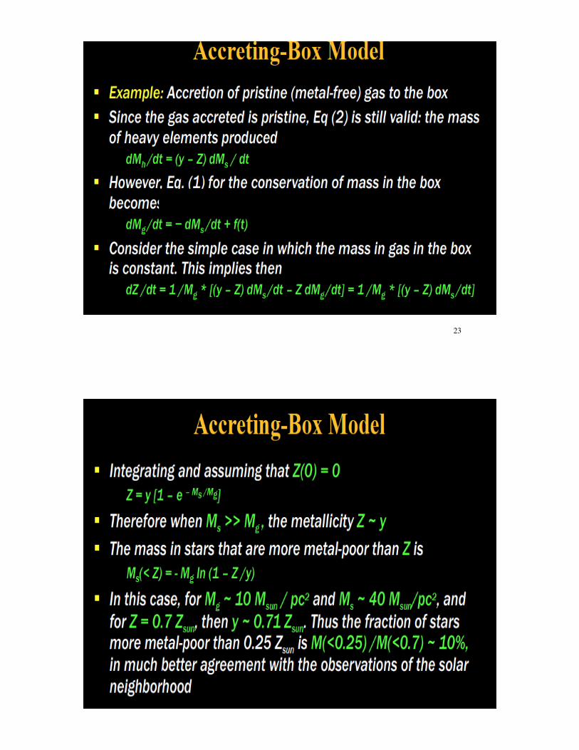
23

24

•  Simple closed-box model works well for bulge of Milky Way

•  Outflow and/or accretion is needed to explain

Metallicity distribution of stars in Milky Way diskMass-metallicity relation of local star-forming galaxies Metallicity-radius relation in disk galaxies Merger-induced starburst galaxiesMass-metallicity relation in distant star-forming galaxies

25

Galactic bulge metallicity distributions of stars S&G fig 4.16- solid line is closed box model

Leaky box Outflow and/or accretion is needed to

explain•  Metallicity distribution of stars in

Milky Way disk•  Mass-metallicity relation of local star-

forming galaxies

•  In a growing universe (remember galaxy masses increase with time) expect gas inflow

•  Gas outflow could be caused by the effects of star formation (supernova) and active galaxies injecting huge amounts of energy

26

27

28

29

30

31

Optical Image of LMC and SMC

Magellanic Clouds •  Satellites of the MW: potentially

dynamics of SMC and LMC and the Magellanic stream can allow detailed measurement of mass of the MW.

•  LMC D~50kpc Mgas ~ 0.6x109 M¤ (~10% of Milky Way)Supernova rate ~0.2 of Milky Way

R.C. Bruens

Magellanic stream-tidally removed gas??

Position of LMC and SMC over time- in full up dynamical model;no merger with MW in 2 Gyrs ?

32

Dynamical Friction •  Transfer of energy of the forward motion of the galaxies into internal

energy (e.g. motion of test particles inside the galaxies)•  this drag force, is called dynamical friction, which transfers energy

and momentum from the subject mass to the field particles. •  Intuitively, this can be understood from the fact that two-body

encounters cause particles to exchange energies in such a way that the system evolves towards thermodynamic equilibrium.

•  The set-up is an infalling galaxy of mass Ms moves into a large collisionless object whose constituents have mass m<< Ms

•  Thus, in a system with multiple populations, each with a different particle mass mi, two-body encounters drive the system towards equipartition, in which the mean kinetic energy per particle is locally the same for each population: m1<v1

2> = m2<v22>

33

Dynamical Friction Derivation pg 285 S&G•  As M moves past it gets a change in

velocity in the perpendicular direction δV=2Gm/bV (in the limit that b

>>2G(M+m)/V2

momentum is conserved so change in kinetic energy in the perpendicular direction is

δ(KE)=(M/2)(2Gm/bV)2+(m/2)(2GM/bV)2=

2G2mM(M+m)/b2V2 (eq 7.5 S&G)δV~[2G2m(M+m)/b2V3]and dV/dt~4πG2[(M+m)/V2]

notice that the smaller object acquires the most energy- which can only come from the forward motion of galaxy M

34

Dynamical Friction-cont•  basically this process allows the exchange of energy between a smaller 'incoming'

mass and the larger host galaxy •  The smaller object acquires more energy

–  -removes energy from the directed motion small particles (e.g. stars) and transfers it to random motion (heat) - incoming galaxy 'bloats' and it loses stars.

•  It is not identical to hydrodynamic drag:–  in the low velocity limit the force is ~velocity, while in the high limit is goes as

v-2 •  independent of the mass of the particles but depends on their total density- e.g.

massive satellite slowed more quickly than a small one

35

Analytic Estimate How Fast Will Local Group Merge?•  Dynamical friction (S+G 7.1.1 )-occurs when an object has a relative

velocity wrt to a stationary set of masses. The moving stars are deflected slightly, producing a higher density 'downstream'- producing a net drag on the moving particles

•  Net force =Mdv/dt~ 4π G2M+m)nm/V2 (eq 7.8) for particles of equal mass m and number n-so time to 'lose' significant energy-timescale for dynamical friction-slower galaxy moves, larger its deacceleration a more massive satellite is slowed more quickly

•  tfriction~V/(dv/dt)~V3/4πG2Mmρ/lnΛ (in previous lecture)Μ∼1010 Μ;m=1Μ; ρ∼3x10�4 Μ/pc3 Galactic density at distance of LMC (problem 7.6)

putting in typical values for LMC

tfriction~3Gyrs

36

•  Accurate estimates of the effects of dynamical friction and the timescale for an orbiting satellite to lose its energy and angular momentum to merge with a host are essential for many astrophysical problems.

•  the growth of galaxies depends on their dynamical evolution within larger dark matter halos.

•  dynamical friction provides a critical link between dark matter halo mergers and the galaxy mergers that determine, e.g., stellar masses, supermassive black hole masses, galaxy colors, and galaxy morphologies. (Boylan-Kolchin et al 2007)

37

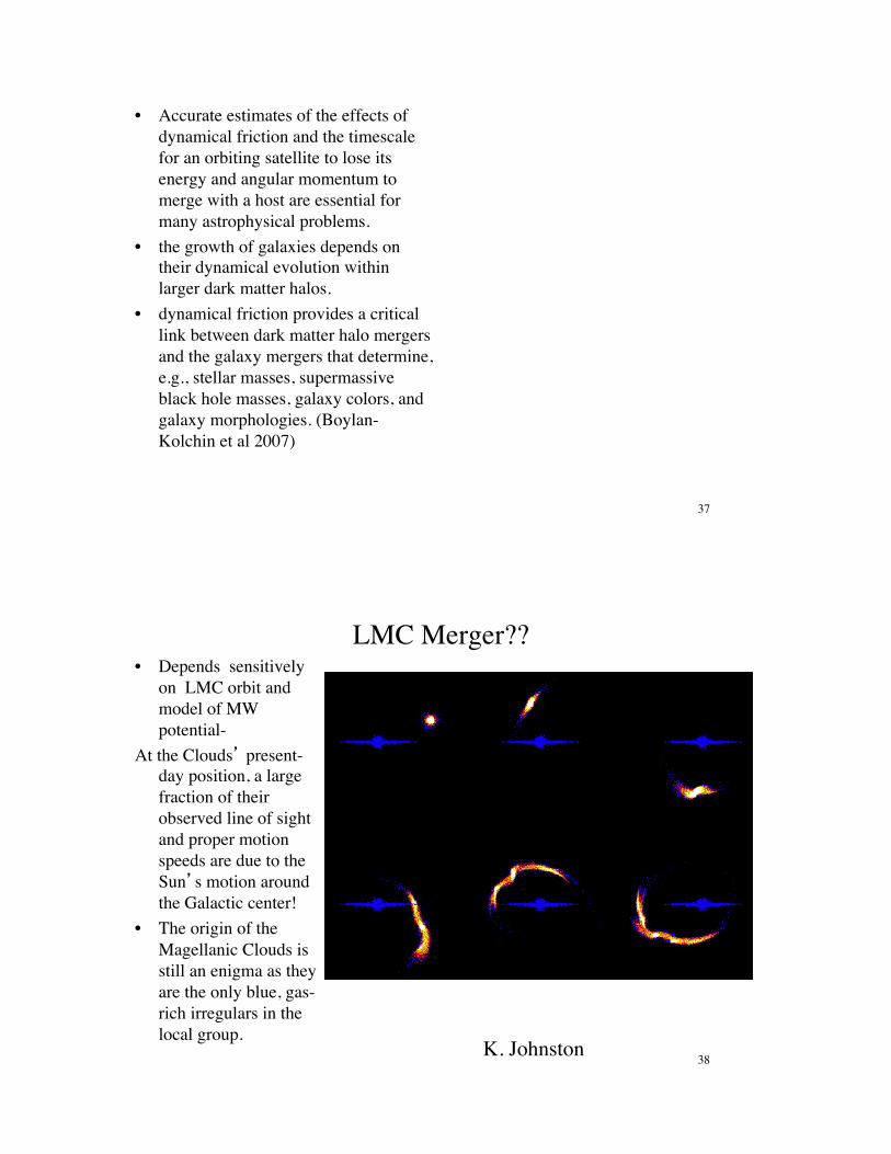
LMC Merger??•  Depends sensitively

on LMC orbit and model of MW potential-

At the Clouds� present-day position, a large fraction of their observed line of sight and proper motion speeds are due to the Sun�s motion around the Galactic center!

•  The origin of the Magellanic Clouds is still an enigma as they are the only blue, gas-rich irregulars in the local group.

K. Johnston 38

To get orbit to MCs need all 6 quantitites (x,y,z) and vx,vy,vzmeasure positon and radial velocity easytangent velocity is hard recent results differ a lovx,vy,vz[km/s] 41±44, -200±31, 169±37Kroupa & Bastian (1997)vx,vy,vz[km/s] -56±39, -219±23, 186±35

van der Marel et al. (2002)

Need distance to convert angular coordinatesto physical units

Dynamical friction vectors-depend on shape and size of MW dark halo!

39

Distance to LMC•  LMC is unique in that many Cepheids

can be detected in a galaxy with rather different metallicity with no effect of crowding

distance modulus, µ,(log d=1+µ/5) pc LMC µ= 18.48 ± 0.04 mag; (49.65 Kpc)

This sets the distance scale for comparison with Cepheids in nearbygalaxies (Freedman+Madore 2010)

LMC Distance Modulus

log Period (days)

abso

lute

mag

in e

ach

band

Rela

tive

prob

abili

ty

40

Rotation of the LMC New result from Gaia•  Each vector shows motion of stars

over next 7.2Myr•  Big vector is overall motion of LMC

(van den Marel and Sahlmann 2017)•  Proper motion is ~ 1mas/yr and

velocities are in km/sec to connect the 2 need distance.

•  Fit gives m-M=18.54 mag or D= 51 kpc

41

3D Map of LMC/SMC•  Data so precise get 3D 'map' of LMC/SMC

42

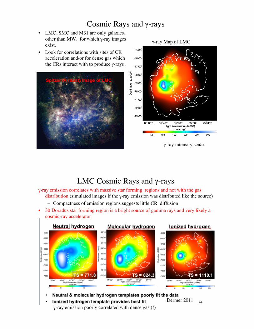
Cosmic Rays and γ-rays•  LMC, SMC and M31 are only galaxies,

other than MW, for which γ-ray images exist.

•  Look for correlations with sites of CR acceleration and/or for dense gas which the CRs interact with to produce γ-rays .

Spitzer IR (dust) Image of LMC

γ-ray Map of LMC

γ-ray intensity scale 43

LMC Cosmic Rays and γ-raysγ-ray emission correlates with massive star forming regions and not with the gas

distribution (simulated images if the γ-ray emission was distributed like the source) –  Compactness of emission regions suggests little CR diffusion

•  30 Doradus star forming region is a bright source of gamma rays and very likely a cosmic-ray accelerator

Dermer 2011γ-ray emission poorly correlated with dense gas (!)

44