location theory and strategic supply chain management ws 0809... · facility location and strategic...

Facility Location and Strategic Supply Chain Management

Prof. Dr. Stefan Nickel

Location Theory and Strategic Supply Chain Management

Structure

I. Location ConceptsChapter 1 – IntroductionChapter 2 – Economic and Descriptive Facility

Location Models



Location Concepts

Chapter 2 – Economic and Descriptive Facility Location Models

Contents

• Economical Facility Location Models- Theory of Land Values- Home Location Decisions with Minimal Costs- Theory of Land Utilization

• Descriptive Interplant Facility Location Models

• Competitive Facility Location Planning



Theory of land values

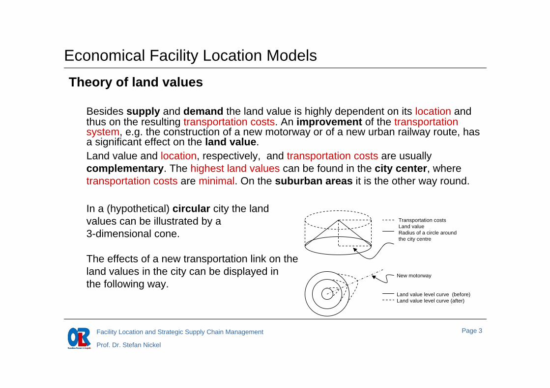
Besides supply and demand the land value is highly dependent on its location and thus on the resulting transportation costs. An improvement of the transportation system, e.g. the construction of a new motorway or of a new urban railway route, has a significant effect on the land value.Land value and location, respectively, and transportation costs are usually complementary. The highest land values can be found in the city center, where transportation costs are minimal. On the suburban areas it is the other way round.

In a (hypothetical) circular city the landvalues can be illustrated by a3-dimensional cone.

The effects of a new transportation link on theland values in the city can be displayed inthe following way.

Economical Facility Location Models

Transportation costsLand valueRadius of a circle around the city centre

New motorway

Land value level curve (before) Land value level curve (after)



Home location decisions with minimal costs

Typically, households try to find a location which minimizes rent and transportation costs.

Simplified, these location costs can be described as

where • d denotes the distance from the location to the city center• C(d) denotes the total location costs• Q denotes the given size of living space• p(d) denotes the location-dependent rent per unit of living space, e.g. per sqm• V denotes the number of trips to the city center, e.g. for work, for shopping• k(d) denotes the location-dependent transportation costs

Economical Facility Location Models



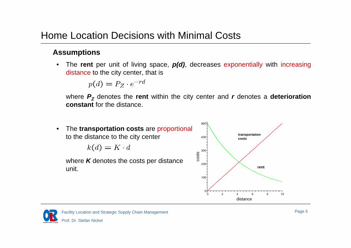
Assumptions• The rent per unit of living space, p(d), decreases exponentially with increasing

distance to the city center, that is

where PZ denotes the rent within the city center and r denotes a deterioration constant for the distance.

• The transportation costs are proportionalto the distance to the city center

where K denotes the costs per distanceunit.

Home Location Decisions with Minimal Costs

transportation costs

rent

distanceco

sts



Under these assumptions the minimum cost location can be found by minimizing the function C(d).

After differentiating the function C with respect to d and setting the differentiated function to zero one receives the optimal distance d* with

ExampleConsider a household with thefollowing parameters• Q = 50 m2, PZ = 10 €, r = 0.2• V = 100, K = 0.5 €

The minimum isd* = 3.47 and C(d*) = 423.29

Home Location Decisions with Minimal Costs

(3.47, 423.29)

distance

cost

s



Economical Approaches

Theory of land utilization

Whereas the question of facility location theory is:

„Where should a certain activity be located?“

the theory of land utilization asks

„Which activity should be established at a certain location?“

Examples for activities are • Buildings and facilities• Types of cultivation of land• Production of goods• Offering a service



Theory of Land Utilization

Von Thünen‘s Model

Von Thünen made the following assumptions for his model• The area of interest is a circular, "Isolated State“ with steady productivity.• The city is located centrally within this state. • All transportation link are of similar quality.• One can produce goods everywhere at the same costs.• Transportation costs increase in proportion to the distance.• A set of production activities and their outputs are given.

According to profit maximization, the main question is: “Which goods should be produced in which distance to the market?”




Example with two production activitiesAssume that

• p1 and p2 denote the prices of products P1 and P2, minus all the production costs• d denotes the distance from the chosen location to the market in the center • k1 and k2 denote the transportation costs per distance unit of P1 and P2.

The profit R1(d) achieved by the production of good 1 in distance d is given by the function

As a consequence the production of P1becomes unprofitable if the distance increasesbeyond .

d

R(d)

R1(d) = p1 - k1d

d1max

p1



Theory of Land UtilizationOther interpretations of R(d)

R(d) is the maximum price that a producer is willing to pay for a property in distance d to the center. So this is the producer’s maximum bid at an auction.In this context R(d) is called „bid-rent“.

Now we examine the second good and its profit function.

There are two different cases • Producing one good is everywhere

at least as profitable as the production ofthe other one

that is good 1 „dominates“ good 2.

Therefore only P1 would be producedwithin the interval . d

R1(d)

R1(d)

p1

p2

R2(d)

Good 1d1

max



Theory of Land Utilization• There is no domination of the goods. Which means that there are distance areas

for both goods where the production of one good is more profitable than that of the other one.From this it follows that there is a distance d12 where the production of both goodshave the same profitability.

For example

To maximize the profit one would producegood 1 only in the circle from the center tod12 and in the circle from d12 to dmax onlygood 2.

d

R(d)

R1(d)p1

p2

R2(d)

d12

Good 1

Good 2 d2max



Theory of Land UtilizationThe distance d12, where both goods, P1 and P2, have the same profit, results from the intersection (d12, R1/2(d12 )) of the profit functions

If d12 ≤ 0 or d12 ≥ min {d1max, d2

max} then one good is dominated by the other.

d

R(d)

R1(d)

p1

p2R2(d)

d12Good 1

d1max

d2max

d

R(d)

R1(d)

p1

p2

R2(d)

Good 1d12



Theory of Land UtilizationThe general case

n different activities i, i = 1,…, n, with different prices pi and different transportationcosts ki are given.

The maximum profit for a certain distance d from the center is defined as

The maximum distance for a profitable production is defined as

Now we are looking for a profit maximizing layout of activities in a distance between 0 and dmax to the center.



Theory of Land UtilizationIf one determines the distance interval where the production of Pi is more profitable than the one of any other good, that means

it follows directly the considered profit maximizing layout .

To calculate these distance intervals one has to determine the intersections of the profit functions of Pi and Pj , for which the following assumption holds

That means intersections whichyield to a maximally possible profitfor this distance without beingdominated by other more profitableproduction activities.

d

R(d)

p1

p2

max. profit

dominated




Method (for computing the upper envelope)1. Formulate the corresponding profit function for every production activity.

Set d‘ = 0 and I = {1,…,n}.

2. Determine Ri*(0) = maxj=1,…,n Rj(0), that is the most profitable activity in the center Pi*.If there is no unique maximum, choose that one among the most profitable activities with the lowest kj. Set I = I \ {i*} and store i* in a list L.

3. Intersect Ri*(·) with all Rj(·), j ∈ I, and determine the intersection pointSi*,j = (di*,j , Ri*/j(di*,j )) with the lowest value di*,j > d‘.Set d‘ = di*,j , i* = j and I = I \ {i*}. Add d‘ and i* at the end of list L.

4. Repeat step 3 until there are no further intersections or I = {}.Add dmax at the end of L.

List L contains now the desired distance intervals and the respective profitable production activities.



Theory of Land UtilizationExample

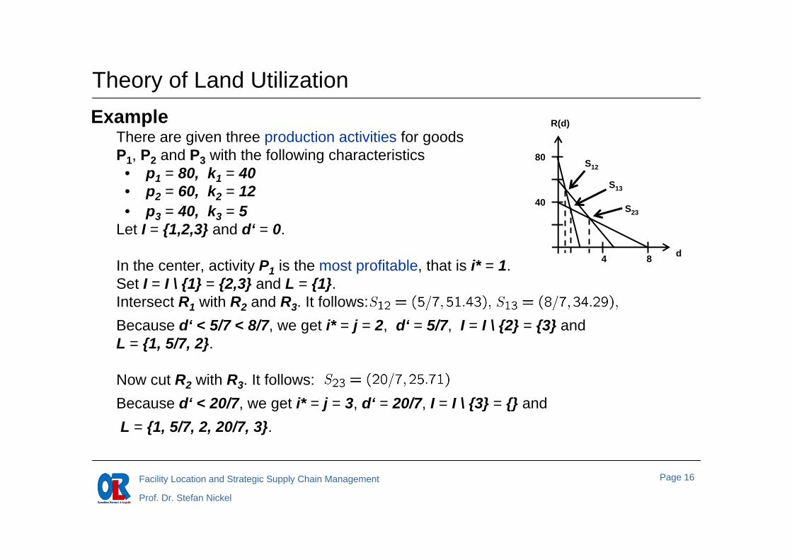
There are given three production activities for goodsP1, P2 and P3 with the following characteristics

• p1 = 80, k1 = 40• p2 = 60, k2 = 12• p3 = 40, k3 = 5

Let I = {1,2,3} and d‘ = 0.

In the center, activity P1 is the most profitable, that is i* = 1. Set I = I \ {1} = {2,3} and L = {1}.Intersect R1 with R2 and R3. It follows:Because d‘ < 5/7 < 8/7, we get i* = j = 2, d‘ = 5/7, I = I \ {2} = {3} and L = {1, 5/7, 2}.

Now cut R2 with R3. It follows:Because d‘ < 20/7, we get i* = j = 3, d‘ = 20/7, I = I \ {3} = {} andL = {1, 5/7, 2, 20/7, 3}.

d

R(d)

80

40

4 8

S12

S13

S23



Theory of Land Utilization: ExampleBecause I = {}, add dmax = 8 to L and stop.

Result: L = {1, 5/7, 2, 20/7, 3, 8}.

That’s why in circle [0, 5/7] good 1 is the most profitable one. After that P2 earns the highest profit, R(d) = R2(d), d ∈ [5/7, 20/7]. And good 3 is in circle [20/7, 8] most profitable.

NoteThe method can be extended to more complex, non-linear productionsand transportation cost functions.

d

R(d)

80

40

4 8

S12

S13

S23



Location Concepts


Contents

• Economical Facility Location Models

• Descriptive Interplant Facility Location Models- Checklist Method

- Scoring Method

• Competitive Facility Location Planning



Chapter 2 – Economical and Descriptive Facility Location Models

Descriptive Interplant Facility Location Models

Both checklist and scoring methods determine the best location for a new facility based on location factors.

The methods assume • a limited number of location alternatives• a user-defined number of location factors

Checklist MethodProcedure

• Combination of adequate location factors that are relevant for the problem. Thereby, one has to be very careful.

• For every relevant location factor, one has to check and mark (e.g. with a cross) which location will fulfill the factor best.



In this procedure some locations may get multiple marks and therefore seem to be very advantageous whereas others will get nothing.

ExampleThere are given 6 locations, A – F, and 6 relevant factors, I – VI. For each relevant location factor, the best alternatives are marked with a cross.

Checklist Method

location relevant location factorsI II III IV V VI

A XB X XC XDE XF X

Location B is most suitable



Checklist MethodAdvantages

The checklist method provides a qualitative basis for a systematical analysis of facility location problems and restricts the decision space. It forces to a requires a careful consideration of the problem and leads to the elimination of “impossible” locations or to the accentuation of “advantageous” alternatives.

DisadvantagesThe checklist method doesn’t provide a basis for a unique facility location decisionfor different reasons:

• First of all the selection of relevant location factors will always be subjective; moreover, the chosen location factors will neither describe the problem completely nor will they be independent.

• Furthermore one has to criticize the marking technique because subjective moments and uncertain future expectations have a great influence on the decision.

• At least the lack of differentiation between different degrees of performance for the location factors is a great shortcoming.



Descriptive interplant facility location models

Scoring Method

This method uses some quantifications.

Steps of the method• Identification of suitable location factors.• Determination of a weight for every location factor which represents the relative

importance in comparison with the other location factors.• It has to be checked how much of the relevant location factors will be satisfied at

a location. The result is expressed by numbers that represent rankings or point scores. In this connection a high rank is related to a high degree of performance.

• The ranks are multiplied by the according weights to get ratings. The sum of all ratings leads to a total rating for every location.

The location with the highest total rating is called optimal.



Scoring MethodExample

There are given 6 locations, A - F, and 2 location factors, I and II, in combination with the according weights, rankings and the resulting ratings.

Location D, which offers the highest total rating, is optimal.

LocationLocation Factor I Location Factor II

Total RatingRank Weight Rating Rank Weight Rating

A 2 0.3 0.6 4 0.7 2.8 3.4B 1 0.3 0.3 2 0.7 1.4 1.7C 3 0.3 0.9 1 0.7 0.7 1.6D 4 0.3 1.2 6 0.7 4.2 5.4E 5 0.3 1.5 5 0.7 3.5 5.0F 6 0.3 1.8 3 0.7 2.1 3.9



Scoring MethodAdvantages

The scoring method comprises from the analysis of a facility location problem to the facility location decision. The usage of weights and rankings makes the method widely transparent.The method divides the decision process into several steps, reduces the subjectivity concerning the decision and uses the given information as good as possible.

DisadvantagesDespite of the better quantification, in comparison with the checklist method, a little subjectivity remains.Furthermore the determination of relevant location factors is still problematic.

Because the method can be generally applied and is easy to handle, it has a great importance in practice.

In both methods the difficulties basically result from several, partially non-quantifiable location factors.



Location Concepts


Contents



• Competitive Facility Location Planning- Single Sourcing- Models with Partitioning

- Leader – Follower Models



Economic and Descriptive Facility Location ModelsCompetitive Facility Location Planning

The objective of Competitive Facility Location Planning is to locate one or several new facilities so that the market share and the profit of the own company will be maximized.

Typical examples are the location of• Retail stores or branches of a bank• Department stores• Movie theatres

The computation of the market share achieved by the own facilities plays a very important role in these models.

Most relevant is the correct description of customer behaviors, that means how the customer demand (e.g. buying power, number of habitants, demand for a special good) is distributed among the competing facilities.



Competitive Facility Location PlanningConcerning the customer behavior one basically distinguishes two models.

Models with single sourcing allocation: „All or nothing“The demand of a customer is completely satisfied by exactly one facility.

One will, for example, always go to the branch bank around the corner whether at home or at work.

Models with partial allocationThe customers distribute their demand pro rata on several facilities.

For instance one buys small quantities of food in the closest shop, but one drives to the next supermarket in order to buy in bulk.



Competitive Facility Location Planning

Single Sourcing Allocation

In these models one can exactly decide which facility is the best or most attractive for a customer.

Vice versa the market area of a facility is exactly determined. The market area is that part of the whole market that is completely served by one facility.

The market areas represent a (disjoint and completely covering) partition of the whole market.

Most models to predict the best facility location are based on:• Distance between customer and facility, e.g. in km.• Costs, for satisfying the demand, e.g. transportation and product costs.• Utility of the different facilities for the customer.



Single Sourcing

Market Areas Based on Euclidean Distance Consider the plane IR2 as the market area and two companies A and B each with one store at the location xA and xB respectively.

What do the market areas MAA and MAB of the two stores look like?

A customer in x ∈ IR2 will always satisfy his demand at the nearest store. Hence, he will visit xA of company A, if the distance between x and xA is smaller than the one between x and xB

Therefore, the market area MAA of the store at the location xA contains all the points which are closer to xA than to xB

Analogously for MAB.



Market Areas Based on Euclidean Distance If the customer lives equidistant to both stores,

then the customer will be indifferent towards both.

The set of all points that are equidistant to both locations, xA and xB ,is called indifference set ISAB.

The indifference set is the boundary between the set of all points closer to xA thanto xB, and the set of all points closer to xB than to xA.

In case of the Euclidean Distance the indifference set is theperpendicular bisector of theline segment connecting xA and xB.

xA

xB



Market Areas Based on Euclidean Distance

xA

xB

xC

If we add a third competitor C with a storelocated in xC, the partition of the market wouldchange as follows

This type of partition is called Voronoi-Partition and the figurewhich describes the borderlines between the market areas is called Voronoi-Diagram.



Single Sourcing

Market Areas Based on CostsAlready in 1882 Launhardt dealt with the structure of market areas in the case oftwo competing companies in the plane.

The basis of his analysis was the assumption that the customer buys the desired good in that store which charges the lowest price.

The lowest price p(x) at location x is computed in the following way

where- pA/B denotes the product costs and- kA/B denotes the transportation costs per distance unit.



Illustration for two stores located in xA and xB

The iso-price lines for the stores, that is the set of all points with identical prices, are concentric circles around the respective locations.

Thereby it holds that with increasingtransportation costs, the iso-price linesbecome more dense.

The indifference set, that is the set of allpoints with identical costs, is given by the solution of the equation

In case of kA ≠ kB the indifference setis a closed curve.

Thereby the market area of the company with the higher transportation costs will always be bounded.

Market Areas Based on Costs

indifference curve

xA xB



If one illustrates the price levels in the market areaone can see that the indifference set is describedby the intersection of two cones, the so called Launhardt Cones.

If the transportation costs of both companies areidentical, kA = kB, then the respective market areas are unbounded.

If additionally holds pA = pB, then the costs could be reduced to the distance and one gets the case of distance-based market areas.

Market areas based on costs

indifference curve

xA xB



Single Sourcing

Hotelling’s Model

The first acknowledged modern approach about Competitive Facility Location Planning is the paper of Hotelling, 1929. He studied the case of two competing companies on a restricted, linear market.

He made the following assumptions- The considered market is a closed interval [c, d ]- The demand (buying power) is constant and evenly distributed over the interval- The cost factors of both companies are identical- Customers always satisfy their demand at the nearest facility- Both competitors can replace their facility as often as they want to, but they

can’t choose the same location simultaneously

A classic example is the case of two ice-crème vendors that compete for the costumers on a beach.



Hotelling’s Model

ProcedureThe first candidate, e.g. company A,that locates his facility wins the complete market.

The market area of company A is the complete interval and the market share is D (d – c).

Next, company B will locate itsfacility such, that it gains an asbig as possible market share.

The borderline, that is the indifference set ISAB, between the two market areas is a single point.

The according market areas are [c, ISAB ] and [ISAB , d].

xA

MAA

c d

xA

MAA

c dxB

MAB

ISAB



Hotelling‘s ModelThe market share MSA and MSB respectively for both competitors is calculated as the product of the constant demand and the size of the respective market area.

To maximize the market area and in that way the market share MSB, company Bwill locate its new facility xB directly on the left or on the right side of facility location xA of the first competitor. The side depends on which partial interval is bigger. In our example, the best location is directly on the right side.

After locating the facility of company B, A can relocate its facility. To maximize its market share it follows the same considerations as for company B in the step before. In the example A locates its facility directly on the right side of xB.

xA

MAA

c dxB

MAB

xA

MAB

c dxB

MAA



Hotelling’s ModelThis game will be repeated as long as one of the competitors can still improve its market share.

An equilibrium-state is reached, when both competitors are directly placed on theleft and on the right side of the center of the interval, respectively.In this case both companies divide the market in equal shares among each other.

Further replacements would only reduce their market shares.

Over the years, the basic model of Hotelling has been extended and adjusted to the reality, i.e.

- different company-dependent cost types- variable demand, that is dependent on the distance between the customer and

the next facility

xB

MAA

c dxA

MAB



Location Concepts


Contents



• Competitive Facility Location Planning- Single Sourcing

- Models with Partitioning- Leader – Follower Models




Models with partitioningIn these models the customers distribute their demand pro rata on several facilities.

Gravity ModelsThese models consider the gravitational pull, that means the attraction that acertain location has for a customer. Based on that gravity the probability that a customer will visit the facility and how much demand he will satisfy there is calculated.For this reason a customer will normally not satisfy his total demand at one single facility, but will proportionally distribute his demand on several facilities.As a consequence, the market areas of different facilities are overlapping and can’t be clearly differentiated.



Gravity-ModelsGravity-Models are applied in situations, where the premise of clear assignment, e.g. to the next or cheapest facility, can not be justified.

The gravity is normally positively affected by the attractiveness of a facility at a location and negatively by the distance to the customer.

Criteria for the attractiveness are classified as

• Location dependent criteria- Size of the parking lot- Location and accessibility- Connection to public transport

• Facility dependent criteria- Size of the sales area- Prices- Size and quality of the range of goods



Gravity-Models

Huff’s ModelHuff was the first author who considered gravity models in detail.

He proposed that every facility at a location exerts a gravity on a customer and this gravity is

- proportional to the size of the sales area of the facility and - reciprocally proportional to a potency of the distance between both locations

Thus:

where- A(E, K) denotes the gravity of the facility E on a customer K- wE denotes the size of the facility E at this location- d (K, E ) denotes the distance from customer K to the location of facility E- r denotes a potency (deterioration factor) for the distance



Huff’s Model

Note:If the locations of customer K and facility E are identical the facility’s gravity is “infinite”. As a result the demand of the customer will be satisfied totally by the facility.

Illustration of the gravity function asa function of the distance betweenthe customer and a facility locationin point (5, 5).

Due to this formulation, which is identical to the formulation for the calculation of the gravitational pull between two planets, the name gravity model is derived.



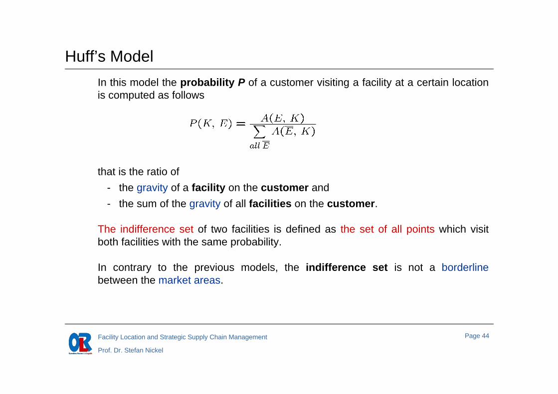
Huff’s ModelIn this model the probability P of a customer visiting a facility at a certain location is computed as follows

that is the ratio of - the gravity of a facility on the customer and - the sum of the gravity of all facilities on the customer.

The indifference set of two facilities is defined as the set of all points which visit both facilities with the same probability.

In contrary to the previous models, the indifference set is not a borderline between the market areas.



Huff’s ModelThe demand share of a customer that is satisfied at a certain facility results from the product of the total demand of the customer and the probability of visiting:

Assuming that there is just a discrete number of customer locations, the total demand of a facility is the sum of all shares of customer demand which are satisfied at this facility:

Therefore, the total market share of the facility is:



Huff’s ModelIf a new facility has to be located within the market, one will choose a location that maximizes the ratio of the sum of the market shares of the own existingfacilities plus the new facility and the sum of all customer demands:



Huff’s Model

Example for a linear restricted market

Consider the market [0, 10] and two companies A and B located in xA = 2 and xB = 7 respectively as well as the sizes of the sales areas wA = 5 and wB = 7. Let the deterioration factor be constantly 2, which means that the gravity is decreasing quadratically with the distance.

The probabilities resulting from the customer location x = 4 are as follows

Illustration of the probabilities for both facilitiesas functions subject to the customer location x.

and

xA xB



Gravity ModelsOver the years Huff’s model has been extended and adjusted step by step to practice.

One of the amjor extensions considers the size of the sales area as a measure for the attractiveness. It has been replaced by complex combinations of criteria for the attractiveness.

E.g. in the „multiplicative competitive interaction“ (Nakanishi und Cooper, 1974) the total attractiveness of a facility at a location is computed by the product of several attractiveness-factors where every factor is additionally raised to a higher power.

Because of their flexibility these models are extensively applied in practice.



Location Concepts


Contents



• Competitive Facility Location Planning- Single Sourcing

- Models with Partitioning

- Leader – Follower Models




Leader – Follower Models

In these models two competitors are locating new facilities one after the other in a new (unexplored) market.

Thereby leader L is first to choose the locations for all his facilities and then it is the follower’s F turn.

The facility location choices of L and F are interacting.

Followerdoes not have to choose his facility location strategy untill the leader L has made his facility location choice.

Leaderhas the problem that he does not know the facility location strategy of F.



Leader – Follower ModelsTypical strategies for F

AggressiveLocate new facilities in a way that L loses as much market share as possible.(thus the own market share is subordinate)

Profit – MaximizingLocate new facilities in a way that the own market share is maximized.

NeutralLocate new facilities according to other criteria.



Leader – Follower ModelsUnder this point of view there are several strategies for L.

Maxi – MinL locates new facilities such that he maximizes his market share when F applies an aggressive strategy, that is that F aims on minimizing the market share of L.

Min – Regret L locates new facilities such that the gain of market share with a possible replacement of facilities (after the choice of F) becomes minimal whatever the location choice of F will be.

Max – Profit (Van Stackelberg)L locates new facilities in such a way that his market share is maximized when Falso applies a profit-maximizing strategy.



Leader – Follower ModelsExamples in Plastria, Vanhaverbeke, 2004

Consider a quadratic 10x10 market with two demand-clusters.

The demand is uniformly distributedin the first cluster [30, 50] andthe second [80, 100], respectively .

Catchment area: 2.5 distance unitsThat means that the market areas have the following shape



ExamplesAssumption

L has the budget for two new facilities, F just for one.

Optimal locations, that means market share-maximizing ones if L is alone on the market.

Achieved market share: 3130



ExamplesSeveral strategies and achieved market shares

Note to Min – RegretThe follower-location is the one with maximal regret.

Maxi – Min Min – Regret Van Stackelberg

Leader: 2341Follower: 876





ExamplesFlandern

PopulationInhabitants: 6 653 780

Land pricesAverage: 149 € / m2



ExamplesVan Stackelberg

Leader: Budget is sufficient for 4 facilitiesAchieved market share:

3 316 010 (50%)

Follower: just one facilityAchieved market share:

2 416 820 (36%)

location theory and strategic supply chain management ws 0809... · facility location and strategic...

Documents