arX

iv:0

811.

2690

v1 [

nlin

.CG

] 1

7 N

ov 2

008

A framework for the local information dynamics of distributed computation in

complex systems

Joseph T. Lizier,1, 2, ∗ Mikhail Prokopenko,1 and Albert Y. Zomaya2

1CSIRO Information and Communications Technology Centre,Locked Bag 17, North Ryde, NSW 1670, Australia

2School of Information Technologies, The University of Sydney, NSW 2006, Australia(Dated: November 17, 2008)

The nature of distributed computation has often been described in terms of the component op-erations of universal computation: information storage, transfer and modification. We introducethe first complete framework that quantifies each of these individual information dynamics on alocal scale within a system, and describes the manner in which they interact to create non-trivialcomputation where “the whole is greater than the sum of the parts”. We apply the framework tocellular automata, a simple yet powerful model of distributed computation. In this application, theframework is demonstrated to be the first to provide quantitative evidence for several importantconjectures about distributed computation in cellular automata: that blinkers embody informationstorage, particles are information transfer agents, and particle collisions are information modifica-tion events. The framework is also used to investigate and contrast the computations conductedby several well-known cellular automata, highlighting the importance of information coherence incomplex computation. Our results provide important quantitative insights into the fundamentalnature of distributed computation and the dynamics of complex systems, as well as impetus for theframework to be applied to the analysis and design of other systems.

PACS numbers: 89.75.Fb, 89.75.Kd, 89.70.Cf, 05.65.+bKeywords: distributed computation, information storage, information transfer, information modification,information theory, complex systems, self-organization, cellular automata, particles, gliders, domains

I. INTRODUCTION

The nature of distributed computation has long beena topic of interest in complex systems science, physics,artificial life and bioinformatics. In particular, emergentcomplex behavior has often been described from the per-spective of computation within the system [1, 2] and hasbeen postulated to be associated with the capability tosupport universal computation [3, 4, 5].

In all of these relevant fields, distributed computationis generally discussed in terms of “memory”, “commu-nication”, and “processing”. Memory refers to the stor-age of information by an agent or process to be used inits future. It has been investigated in coordinated mo-tion in modular robots [6], in the dynamics of inter-eventdistribution times [7], and in synchronization betweencoupled systems [8]. Communication refers to the trans-fer of information between one agent or process and an-other; it has been shown to be of relevance to biologicalsystems (e.g. dipole-dipole interaction in microtubules[9], and in signal transduction by calcium ions [10]), so-cial animals (e.g. schooling behavior in fish [11]), andagent-based systems (e.g. the influence of agents overtheir environments [12], and in inducing emergent neuralstructure [13]). Processing refers to the combination ofstored and/or transmitted information into a new form;it has been discussed in particular for biological neural

∗jlizier@it.usyd.edu.au

networks and models thereof [14, 15, 16, 17] (where ithas been suggested as a potential biological driver), andalso regarding collision-based computing (e.g. [18, 19],and including soliton dynamics and collisions [20]).

Significantly, these terms correspond to the compo-nent operations of Turing universal computation: infor-

mation storage, information transfer (or transmission)and information modification. Yet despite the obviousimportance of these information dynamics, we have noframework for either quantifying them individually or un-derstanding how they interact to give rise to distributedcomputation. Here, we present the first complete frame-work which quantifies each of the information dynam-ics or component operations of computation on a localscale and describes how they inter-relate to produce dis-tributed computation. Our focus on the local scale withinthe system is an important one. Several authors havesuggested that a complex system is better characterizedby studies of its local dynamics than by averaged or over-all measures (e.g. [21, 22]), and indeed here we believethat quantifying and understanding distributed compu-tation will necessitate studying the information dynam-ics and their interplay on a local scale in space and time.Additionally, we suggest that the quantification of the in-dividual information dynamics of computation providesthree axes of complexity within which to investigate andclassify complex systems, allowing deeper insights intothe variety of computation taking place in different sys-tems.

An important focus for discussions on the nature of dis-tributed computation have been cellular automata (CAs)

2

as model systems offering a range of dynamical behav-ior, including supporting complex computations and theability to model complex systems in nature [1]. We se-lect CAs for experimentation here because there is veryclear qualitative observation of emergent structures rep-resenting information storage, transfer and modificationtherein (e.g. [1, 3]). CAs are a critical proving groundfor any theory on the nature of distributed computation:significantly, Von Neumann was known to be a strong be-liever that “a general theory of computation in ‘complexnetworks of automata’ such as cellular automata wouldbe essential both for understanding complex systems innature and for designing artificial complex systems” ([1]describing [23]).

Information theory provides the logical platform forour investigation, and we begin with a summary of themain information-theoretic concepts required. We pro-vide additional background on the qualitative nature ofdistributed computation in CAs, highlighting the oppor-tunity for our framework to provide quantitative insightshere. Subsequently, we consider each component opera-tion of universal computation in turn, and describe howto quantify it locally in a spatiotemporal system. As anapplication, we measure each of these information dy-namics at every point in space-time in several importantCAs. Our framework provides the first complete quan-titative evidence for a well-known set of conjectures onthe emergent structures dominating distributed compu-tation in CAs: that blinkers provide information storage,particles provide information transfer, and particle col-lisions facilitate information modification. Furthermore,our results imply that the coherence of information maybe a defining feature of complex distributed computation.Our findings are significant because these emergent struc-tures of computation in CAs have known analogues inmany physical systems (e.g. solitons and biological pat-tern formation processes), and as such this work will con-tribute to our fundamental understanding of the natureof distributed computation and the dynamics of complexsystems.

II. INFORMATION-THEORETICAL

PRELIMINARIES

Information theory is an obvious tool for quantifyingthe information dynamics involved in distributed com-putation. In fact, information theory has already provento be a useful framework for the design and analysis ofcomplex self-organized systems [24]. Here, we will ex-tend this success to describing distributed computationin complex systems.

We begin by reviewing several necessary informationtheoretic quantities (generally following the formulationin [25]). The fundamental quantity is the Shannon en-

tropy, which represents the uncertainty associated withany measurement x of a random variable X (units in

bits):

HX = −∑

x

p(x) log2 p(x). (1)

The joint entropy of two (or more) random variablesX and Y is a generalization to quantify the uncertaintyof the joint distribution of X and Y :

HX,Y = −∑

x,y

p(x, y) log2 p(x, y). (2)

The conditional entropy of X given Y is the averageuncertainty that remains about x when y is known:

HX|Y = −∑

x,y

p(x, y) log2 p(x|y). (3)

The mutual information between X and Y measuresthe average reduction in uncertainty about x that resultsfrom learning the value of y, or vice versa:

IX;Y =∑

x,y

p(x, y) log2

p(x, y)

p(x)p(y). (4)

IX;Y = HX − HX|Y = HY − HY |X . (5)

The conditional mutual information between X andY given Z is the mutual information between X and Ywhen Z is known:

IX;Y |Z = HX|Z − HX|Y,Z (6)

= HY |Z − HY |X,Z . (7)

The entropy rate is the limiting value of the rate ofchange of the joint entropy over k consecutive states ofX , (i.e. measurements x(k) of the random variable X(k)),as k increases [26]:

HµX = limk→∞

HX(k)

k= lim

k→∞H ′

µX(k), (8)

H ′µX(k) =

HX(k)

k. (9)

The entropy rate can also be expressed as the limitingvalue of the conditional entropy of the next state of X(i.e. measurements xn+1 of the random variable X ′)given knowledge of the previous k states of X (i.e. mea-

surements x(k)n , up to and including time step n, of the

random variable X(k)):

HµX = limk→∞

HX′|X(k) = limk→∞

HµX(k), (10)

HµX(k) = HX(k+1) − HX(k) . (11)

Grassberger [27] first noticed that a slow approachof the entropy rate to its limiting value was a sign ofcomplexity. Formally, Crutchfield and Feldman [26] usethe conditional entropy form of the entropy rate (10)[69]to observe that at a finite block size k, the difference

3

HµX(k) − HµX represents the information carrying ca-pacity in size k-blocks that is due to correlations. Thesum over all k gives the total amount of structure in thesystem, quantified as excess entropy (measured in bits):

EX =

∞∑

k=0

[HµX(k) − HµX ] . (12)

The excess entropy can also be formulated as the mu-tual information between the semi-infinite past and semi-infinite future of the system:

EX = limk→∞

IX(k);X(k+) , (13)

where X(k+) is the random variable (with measurements

x(k+)n+1 ) referring to the k future states of X (from time

step n + 1 onwards). This interpretation is known asthe predictive information [28], as it highlights that theexcess entropy captures the information in a system’spast which is relevant to predicting its future.

III. CELLULAR AUTOMATA

A. Introduction to Cellular Automata

Cellular automata (CA) are discrete dynamical sys-tems consisting of an array of cells which each syn-chronously update their discrete state as a function ofthe states of a fixed number of spatially neighboring cellsusing a uniform rule. Although the behavior of each in-dividual cell is very simple, the (non-linear) interactionsbetween all cells can lead to very intricate global behav-ior meaning CAs have become a classic example of self-organized complex behavior. Of particular importance,CAs have been used to model real-world spatial dynam-ical processes, including fluid flow, earthquakes and bio-logical pattern formation [1].

The neighborhood of a cell used as inputs to its updaterule at each time step is usually some regular configura-tion. In 1D CAs, this means the same range r of cells oneach side and including the current state of the updatingcell. One of the simplest variety of CAs – 1D CAs usingbinary states, deterministic rules and one neighbor on ei-ther side – are known as the Elementary CAs, or ECAs.Example evolutions of ECAs from random initial condi-tions may be seen in Fig. 2(a) and Fig. 6(a). For morecomplete definitions of CAs, including the definition ofthe Wolfram rule number convention for specifying up-date rules, see [29].

Wolfram [4, 29] sought to classify the asymptoticbehavior of CA rules into four classes: I. Homoge-neous state; II. Simple stable or periodic structures; III.Chaotic aperiodic behavior; IV. Complicated localizedstructures, some propagating. Much conjecture remainsas to whether these classes are quantitatively distinguish-able (e.g. see [30]), however they do provide an interest-ing analogy (for discrete state and time) to our knowledge

of dynamical systems, with classes I and II representingordered behavior, class III representing chaotic behavior,and class IV representing complex behavior and consid-ered as lying between the ordered and chaotic classes.

More importantly, the approach seeks to character-ize complex behavior in terms of emergent structure inCAs, surrounding gliders, particles and domains. Quali-tatively, a domain may described as a set of backgroundconfigurations in a CA, for which any given configura-tion will update to another such configuration in the setin the absence of any disturbance. Domains are formallydefined within the framework of computational mechan-ics [22] as spatial process languages in the CA. Particlesare qualitatively considered to be moving elements of co-herent spatiotemporal structure. Gliders are particleswhich repeat periodically in time while moving spatially(repetitive non-moving structures are known as blinkers).Formally, particles are defined within the framework ofcomputational mechanics as a boundary between two do-mains [22]; as such, they can also be termed as domainwalls, though this is typically used with reference to ape-riodic particles.

These emergent structures are more clearly visiblewhen the CA is filtered in some way, using for example ǫ-machines [22], input entropy [31], local information [32],or local statistical complexity [21]. All of these filteringtechniques produce a single filtered view of the structuresin the CA: our measures of local information dynamicswill present several filtered views of the distributed com-putation in a CA. The ECA examples analyzed in thispaper are introduced in Section III C.

B. Computation in Cellular Automata

CAs can be interpreted as undertaking distributedcomputation: it seems fairly clear that “data representedby initial configurations is processed by time evolution”[4]. As such, computation in CAs has been a populartopic for study (see [1]), with a particular focus in ob-serving or constructing (Turing) universal computationin certain CAs. An ability for universal computation isdefined to be where “suitable initial configurations canspecify arbitrary algorithm procedures” in the computingentity, which is capable of “evaluating any (computable)function” [4]. Wolfram conjectured that all class IV com-plex CAs were capable of universal computation [4, 33].He went on to state that prediction in systems exhibitinguniversal computation is limited to explicit simulation ofthe system, as opposed to the availability of any simpleformula or “short-cut”, drawing parallels to the haltingproblem for universal Turing machines [4, 33] which areechoed by Langton [3] and Casti [5]. (Casti extended theanalogy to undecidable statements in formal systems, i.e.Godel’s Theorem). The capability for universal compu-tation has been proven for several CA rules, through thedesign of rules generating elements to (or by identifyingelements which) specifically provide the component op-

4

erations required for universal computation: informationstorage, transmission and modification. Examples hereinclude most notably the Game of Life [34] and ECA rule110 [35]; also see [36] and discussions in [1].

The focus on elements providing information storage,transmission and modification pervades discussion of alltypes of computation in CAs (e.g. also see [19, 37]).Wolfram claimed that in class III CAs information prop-agates over an infinite distance at a finite speed, whilein class IV CAs information propagates irregularly overan infinite range [33]. Langton [3] hypothesized thatcomplex behavior in CAs exhibited the three componentoperations required for universal computation. He sug-gested that the more chaotic a system becomes the moreinformation transmission increases, and the more ordereda system becomes the more information it stores. Com-plex behavior was said to occur at a phase transitionbetween these extremes requiring an intermediate levelof both information storage and transmission: if infor-mation propagates too well, coherent information decaysinto noise. Langton elaborates that transmission of infor-mation means that the “dynamics must provide for thepropagation of information in the form of signals over ar-bitrarily long distances”, and suggests that particles inCAs form the basis of these signals. To complete thequalitative identification of the elements of computationin CAs, he also suggested that blinkers formed the basisof information storage, and collisions between propagat-ing (particles) and static structures (blinkers) “can mod-ify either stored or transmitted information in the sup-port of an overall computation”. Rudimentary attemptswere made at quantifying the average information trans-fer (and to some extent information storage), via mutualinformation (although as discussed later this is a sym-metric measure not capturing directional transfer). Rec-ognizing the importance of the emergent structures tocomputation, several examples exist of attempts to au-tomatically identify CA rules which give rise to particlesand gliders, e.g. [31, 38], suggesting these to be the mostinteresting and complex CA rules.

Several authors however criticize the aforementionedapproaches of attempting to classify CAs in terms oftheir generic behavior or “bulk statistical properties”,suggesting that the wide range of differing dynamics tak-ing place across the CA makes this problematic [1, 22].Gray suggests that there there may indeed be classes ofCAs capable of more complex computation than univer-sal computation alone [30]. More importantly, Hansonand Crutchfield [22] criticize the focus on universal com-putational ability as drawing away from the ability toidentify “generic computational properties”, i.e. a lackof ability for universal computation does not mean a CAis not undertaking any computation at all. Alternatively,these studies suggest that analyzing the rich space-timedynamics within the CA is a more appropriate focus.As such, these and other studies have analyzed the lo-

cal dynamics of intrinsic or other specific computation,focusing on particles facilitating the transfer of informa-

tion and collisions facilitating the information processing.Noteworthy examples here include: the method of apply-ing filters from the domain of computational mechanicsby Hanson and Crutchfield [22]; and analysis using suchcomputational mechanics filters of CA rules selected viaevolutionary computation to perform classification tasksby Mitchell et al [39, 40]. Related are studies whichdeeply investigate the nature of particles and their in-teractions (e.g. particle types and their interaction prod-ucts identified for particular CAs in [40, 41, 42], and rulesestablished for their interaction products in [43]).

Despite such interest, there is no complete frameworkthat locally quantifies the individual information dynam-ics of distributed computation within CAs or other sys-tems. In this study, we outline how the information dy-namics can be locally quantified within the spatiotem-poral structure of a CA. In particular, we describe thedynamics of how information storage and informationtransfer interact to give rise to information processing.Our approach is not to quantify computation or overallcomplexity, nor to identify universal computation or de-termine what is being computed; it is simply intended toquantify the component operations in space-time.

C. Examples of distributed computation in CAs

In this paper, we will examine the computation carriedout by several important ECA rules:

• Class IV complex rules 110 and 54 [29] (see Fig. 4(a)and Fig. 2(a)), both of which exhibit a number ofglider types and collisions. ECA rule 110 is the onlyproven computationally universal ECA rule [35].

• Rules 22 and 30 as representative class III chaoticrules [29] (see rule 22 in Fig. 7(a));

• Rules 18 as a class III rule which contains domainwalls against a chaotic background domain [22, 44].

These CAs each carry out an intrinsic computation ofthe evolution to their ultimate attractor and phase on it(see [31] for a discussion of attractors and state space infinite-sized CAs).

We also examine a CA carrying out a “human-understandable” computational task. φpar is a 1DCA with range r = 3 (Wolfram rule number0xfeedffdec1aaeec0eef000a0e1a020a0) that was evolvedby Mitchell et al [39, 40] to classify whether the initialCA configuration had a majority of 1’s or 0’s by reachinga fixed-point configuration of all 1’s for the former or all0’s for the latter. This CA rule achieved a success rateabove 70% in its task. An example evolution of this CAcan be seen in Fig. 5(a). The CA appears to carry outthis computation using blinkers and domains for informa-tion storage, gliders for information transfer and glidercollisions for information modification. The CA exhibitsan initial emergence of domain regions of all 1’s or all 0’sstoring information about local high densities of either

5

state. Where these domains meet, a checkerboard do-main propagates slowly (1 cell per time step) in both di-rections, transferring information of a soft uncertainty inthis part of the CA. Some “certainty” is provided wherethe checkerboard encounters a blinker boundary between0 and 1 domains, which stores information about a hard

uncertainty in that region of the CA. This results in aninformation modification event where the domain on theopposite side of the blinker to the incoming checkerboardis concluded to represent the higher density state, and isallowed to propagate over the checkerboard. Because ofthe greater certainty attached to this decision, this newinformation transfer occurs at a faster speed (3 cells pertime step); it can overrun checkerboard regions, and infact collisions of opposing types of this strong propaga-tion give rise to the (hard uncertainty) blinker boundariesin the first place. The final configuration is therefore theresult of this distributed computation.

Quantification of the local information dynamics viathese three axes of complexity (information storage,transfer and modification) will provide quite detailed in-sights into the distributed computation carried out in asystem. In all of these CAs we expect local measuresof information storage to highlight blinkers and domainregions, local measures of information transfer to high-light particles (including gliders and domain walls), andlocal measures of information modification to highlightparticle collisions.

This will provide a deeper understanding of computa-tion than single or generic measures of bulk statisticalbehavior, from which conflict often arises in attempts toprovide classification of complex behavior. In particular,we seek clarification on the long-standing debate regard-ing the nature of computation in ECA rule 22. Sugges-tions that rule 22 is complex include the difficulty in es-timating the metric entropy (i.e. temporal entropy rate)for rule 22 in [27], due to “complex long-range effects,similar to a critical phenomenon” [45]. This effectivelycorresponds to an implication that rule 22 has containsan infinite amount of memory (see Section IVA). Also,from an initial condition of only a single “on” cell, rule22 forms a pattern known as the “Sierpinski Gasket” [29]which exhibits clear self-similar structure. Furthermore,rule 22 is a 1D mapping of the 2D Game of Life CA(known to have the capability for universal computation[34]) and in this sense is referred to as “life in one dimen-sion” [46], and complex structure in the language gener-ated by iterations of rule 22 has been identified [47]. Also,we report here that we have investigated the C1 complex-ity measure [48] (an enhanced version of the variance ofthe input entropy [31]) for all ECAs, and found rule 22 toclearly exhibit the largest value of this metric (0.78 bitsto rule 110’s 0.085 bits). On the other hand, suggestionsthat rule 22 is not complex include its high sensitivityto initial conditions leading to Wolfram classifying it asclass III chaotic [29]. Gutowitz and Domain [49] claimthis renders it as chaotic despite the subtle long-rangeeffects it displays, further identifying its fast statistical

convergence, and exponentially long and thin transientsin state space (see [31]). Importantly, no coherent struc-ture (particles, collisions, etc.) is found for rule 22 usinga number of known filters for such structure (e.g. localstatistical complexity [21]): this reflects the paradigmshift to an examination of local dynamics rather thangeneric, overall or averaged analysis. In our approach,we seek to combine this local viewpoint of the dynamicswith a quantitative breakdown of the individual elementsof computation, and will investigate rule 22 in this light.

IV. INFORMATION STORAGE

In this section we outline methods to quantify informa-tion storage. We describe how total information storageis captured by excess entropy, and introduce active in-formation storage to capture the amount of informationstorage that is currently in use. We present the firstapplication of local profiles of both measures to cellularautomata.

A. Excess entropy as total information storage

Although discussion of information storage or memoryin CAs has often focused on periodic structures (par-ticularly in construction of universal Turing machines),information storage does not necessarily entail periodic-ity. The excess entropy (Eq. (12,13)) more broadly en-compasses all types of structure and memory by captur-ing correlations across all lengths of time, including non-linear correlations. It is quite clear from the predictiveinformation formulation of the excess entropy Eq. (13) –as the information from a system’s past that is relevantto predicting its future – that it is a measure of the totalinformation storage in a system.

We use the term single-agent excess entropy to referto measuring the excess entropy for individual agentsor cells using their one-dimensional time series of states.This is a measure of the average memory for each agent.Furthermore, we use the term collective excess entropy torefer to measuring the temporal excess entropy for a col-lective of agents (e.g. a set of neighboring cells in a CA)using their two-dimensional time series of states. Consid-ered as the mutual information between their joint pastand future (i.e. a joint temporal predictive information),this is a measure of the average total memory stored inthe collective (i.e. stored collectively by a set of cells in aCA). Collective excess entropy could be used for exam-ple to quantify the “undiscovered collective memory thatmay present in certain fish schools” [11].

Grassberger studied temporal entropy rate estimatesfor several ECAs in [27, 45] in order to gain insights intotheir excess entropies. These studies estimated temporalentropy rates Hµ,N (k) for spatial blocks of size N as N isincreased. Estimated values of Hµ,N (k) (for N = 1 andin the limit as N → ∞) were cataloged for most ECAs

6

in a table of statistical properties in [50]. Using theseestimates, the studies focused on inferring the collectiveexcess entropies rather than the single-agent excess en-tropies (N = 1). For several rules (including rule 22,studied with Monte Carlo estimates), the temporal en-tropy rate estimates Hµ,N (k) (for N > 1) were concludedto follow a power law decay to their asymptote Hµ,N :

Hµ,N (k) = Hµ,N + C/kα, (14)

with exponent α ≤ 1 (C is a constant). This is signif-icant because with α ≤ 1 the collective excess entropy(known as effective measure complexity in [27]) is diver-gent, implying a highly complex process. This case hasbeen described as “a phenomenon which can occur inmore complex environments”, as with strong long-rangecorrelations a semi-infinite sequence “could store an infi-nite amount of information about its continuation” [51](as per the predictive information form of the excess en-tropy Eq. (13)). Rule 22 was inferred to have Hµ,N = 0and infinite excess entropy, which can be interpreted as aprocess requiring an infinite amount of memory to main-tain an aperiodicity [26]. Alternative methods for com-puting two-dimensional excess entropies, which would beapplicable for computing the collective excess entropy inCAs, were presented by Feldman and Crutchfield in [52].

In attempting to quantify local information dynamicsof distributed computation here, our focus is on infor-mation storage for single agents or cells rather than thejoint information storage across the collective. Were suchpower-law trends to exist for the single-agent case, theymay be more significant than for the collective case: di-vergent collective excess entropy implies that the collec-tive is at least trivially utilizing all of its available mem-ory (and even the chaotic rule 30 exhibits this), whereasdivergent single-agent excess entropy implies that allagents are individually highly utilizing the resources ofthe collective in a highly complex process. One could goon to study the entropy rate convergence for single agents(N = 1)[70], however any findings would be subject tothe problems with overall or averaged measures describedearlier. Again, we emphasize that our focus is on localmeasures in time as well as space, which we present inthe next section.

First though we note that with respect to CAs, whereeach cell has only a finite number of states b and takesdirect influence from only its single past state and thestates of a finite number of neighbors, the meaning of (ei-ther average or local) information storage being greaterlog2 b bits (let alone infinite) in the state “process” of asingle cell is not immediately obvious. Clearly, a cell inan ECA cannot store more than 1 bit of information inisolation. However, the bidirectional communication inCAs effectively allows a cell to store extra information inneighbors (even beyond the immediate neighbors), and tosubsequently retrieve that information from those neigh-bors at a later point in time. While measurement ofthe excess entropy does not explicitly look for such self-influence communicated through neighbors, it is indeed

the method by which a significant portion of informationis channeled. Considering the predictive information in-terpretation in Eq. (13), it is easy to picture self-influencebetween semi-infinite past and future blocks being con-veyed via neighbors (see Fig. 1(a)). This is akin to theuse of stigmergy (indirect communication through theenvironment, e.g. see [53]) to communicate with oneself.

A measurement of more than log2 b bits stored by a cellon average, or indeed an infinite information storage, isthen a perfectly valid result: in an infinite CA, each cellhas access to an infinite amount of neighbors in which tostore information which can later be used to influence itsown future. Note however, that since the storage mediumis shared by all cells, one should not think about the totalmemory as the total number of cells multiplied by thisaverage. The total memory would be properly measuredby the collective excess entropy, which takes into accountthe inherent redundancy here.

B. Local excess entropy

As discussed previously, we now shift focus to localmeasures of information storage, which have the poten-tial to provide more detailed insights into informationstorage structures and their involvement in computationthan single ensemble measures.

The local excess entropy is a measure of how muchinformation a given agent is currently storing at a par-ticular point in time. To derive it, note that the excessentropy of a process is actually the expectation value ofthe local excess entropy for the process at every time step[54].[71] The local excess entropy eX(n+1) of a process issimply the log term from inside the mutual informationexpansion (as per Eq. (4)) of the predictive informationformulation of excess entropy in Eq. (13), evaluated forthe semi-infinite past and future at the given time stepn + 1:

eX(n + 1) = limk→∞

log2

p(x(k)n , x

(k+)n+1 )

p(x(k)n )p(x

(k+)n+1 )

. (15)

Note that the excess entropy is the average of the lo-cal values, EX = 〈eX(n)〉, and that by convention weuse lower-case symbols to denote local values. The limitk → ∞ is an important part of this definition, since cor-relations at all time scales should be included in the com-putation of information storage. Since this is not com-putationally feasible in general, we retain the notationeX(n + 1, k) to denote finite-k estimates of eX(n + 1).

The notation is generalized for lattice systems (such asCAs) with spatially-ordered agents to represent the localexcess entropy for cell Xi at time n + 1 as:

e(i, n + 1) = limk→∞

log2

p(x(k)i,n , x

(k+)i,n+1)

p(x(k)i,n)p(x

(k+)i,n+1)

. (16)

7

(a)Excess Entropy (b)Active Information Storage

FIG. 1: Measures of single-agent information storage in distributed systems. (a) Excess Entropy: total information from thecell’s past that is relevant to predicting its future. (b) Active Information storage: the information storage that is currentlyin use in determining the next state of the cell. The stored information can be conveyed directly through the cell itself or vianeighboring cells.

Again, e(i, n+1, k) is used to denote finite-k estimates ofe(i, n + 1). Local excess entropy is defined for every spa-tiotemporal point (i, n) in the system. (Alternatively, thecollective excess entropy can only be localized in time).

While the average excess entropy is always positive, thelocal excess entropy may in fact be positive or negative,meaning the past history of the cell can either positivelyinform us or actually misinform us about its future. Anobserver is misinformed where the semi-infinite past andfuture are relatively unlikely to be observed together ascompared to their independent likelihoods.

C. Active information storage

The excess entropy measures the total stored informa-tion which will be used at some point in the future ofthe state process of an agent, possibly but not necessar-ily at the next time step n + 1. In examining the localinformation dynamics of computation, we are interestedin how much of the stored information is actually in use

at the next time step. As we will see in Section VI, thisis particularly important in understanding how storedinformation interacts with information transfer in infor-mation processing. As such, we derive active information

storage AX as the average mutual information betweenthe semi-infinite past of the process and its next state,as opposed to its whole (semi-infinite) future:

AX = limk→∞

I(X(k); X ′). (17)

The local active information storage is then a measure ofthe amount of information storage in use by the process

at a particular time-step n + 1:

aX(n + 1) = limk→∞

log2

p(x(k)n , xn+1)

p(x(k)n )p(xn+1)

, (18)

and we have AX = 〈aX(n)〉. We retain the notationaX(n + 1, k) for finite-k estimates. Again, we generalizethe measure for agent Xi in a lattice system as:

a(i, n + 1) = limk→∞

log2

p(x(k)i,n , xi,n+1)

p(x(k)i,n )p(xi,n+1)

, (19)

and use a(i, n + 1, k) to denote finite-k estimates there,noting that the local active information storage is definedfor every spatiotemporal point (i, n) in the lattice system.

The average active information storage will always bepositive (as for the excess entropy), but is bounded aboveby log2 b bits where the agent only takes b discrete states.The local active information storage is not bound in thismanner however, with values larger than log2 b indicatingthat the particular past of an agent provides strong pos-itive information about its next state. Furthermore, thelocal active information storage can be negative, wherethe past history of the agent is actually misinformativeabout its next state. An observer is misinformed wherethe past history and observed next state are relativelyunlikely to occur together as compared to their separateoccurrence.

D. Local information storage results

In order to evaluate the local measures within sampleCA runs, we estimate the required probability distribu-

8

tion functions from CA runs of 10 000 cells, initializedfrom random states, with 600 time steps retained (afterthe first 30 time steps were eliminated to allow the CAto settle). Alternatively, for φpar we used 1000 cells with1000 time steps retained. Periodic boundary conditionswere used. Observations taken at every spatiotemporalpoint in the CA were used in estimating the requiredprobability distribution functions, since the cells in theCA are homogeneous agents. All results were confirmedby at least 10 runs from different initial states.

We make estimates of the measures with finite valuesof k, noting that the insights described here could notbe attained unless a reasonably large value of k was usedin order to capture a large proportion of the correlations.Determination of an appropriate value of k was discussedin [55] for the related transfer entropy measure, presentedin Section V. As a rule of thumb, k should at least belarger than the period of any regular background domainin order to capture the information storage underpinningits continuation.

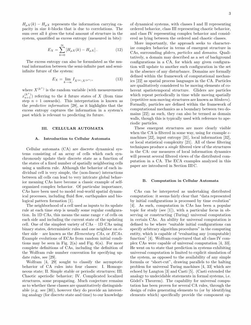
We begin by examining the results for rules 54 and110, which contain regular gliders against periodic back-ground domains. For the CA evolutions in Fig. 2(a)and Fig. 4(a), the local profiles of e(i, n, k = 8) gener-ated are displayed in Fig. 2(b) and Fig. 4(b) (positivevalues only), and the local profiles of a(i, n, k = 16) inFig. 2(c) and Fig. 4(c) (positive values only). It is quiteclear that positive information storage is concentrated inthe vertical gliders or blinkers, and the domain regions.As expected, these results provide quantitative evidencethat the blinkers are the dominant information storageentities. That the domain regions contain significant in-formation storage should not be surprising, since as aperiodic sequence its past does indeed store informationabout its future. In fact, the local values for each mea-sure form spatially and temporally periodic patterns inthe domains, due to the spatial and temporal periodici-ties exhibited there. While the local active informationstorage indicates a similar amount of stored informationin use to compute each space-time point in both the do-main and blinker areas, the local excess entropy reveals alarger total amount of information is stored in the blink-ers. For the blinkers known as α and β in rule 54 [43] thisis because the temporal sequences of the center columnsof the blinkers (0-0-0-1, with e(i, n, k = 8) in the range5.01 to 5.32 bits) are more complex than those in thedomain (0-0-1-1 and 0-1, with e(i, n, k = 8) in the range1.94 to 3.22 bits), even where they are of the same pe-riod. We have e(i, n, k = 8) > 1 bit here due to the dis-tributed information storage supported by bidirectionalcommunication (as discussed earlier): this also supportsthe period-7 domain in rule 110. Another area of stronginformation storage appears to be the “wake” of the morecomplex gliders in rule 110 (see the glider at top left ofFig. 4(b) and Fig. 4(c)). This result aligns well withour observation in [55] that the dynamics following theleading edge of regular gliders consists largely of “non-traveling” information. The presence of the information

storage is shown by both measures, although the relativestrength of the total information storage is again revealedonly by the local excess entropy.

Negative values of a(i, n, k = 16) for rules 54 and 110are displayed in Fig. 2(d) and Fig. 4(d). Interestingly,negative local components of local active informationstorage measure are concentrated in the traveling gliderareas (e.g. γ+ and γ− for rule 54 [43]), providing a goodspatiotemporal filter the glider structure. This is becausewhen a traveling glider is encountered at a given cell, thepast history of that cell (being part of the background do-main) is misinformative about the next state, since thedomain sequence was more likely to continue than be in-terrupted. For example, see the marked positions of the

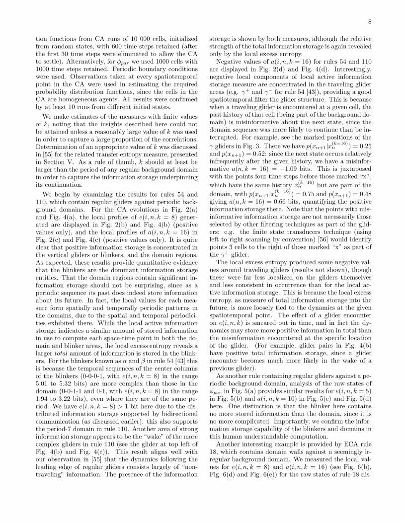
γ gliders in Fig. 3. There we have p(xn+1|x(k=16)n ) = 0.25

and p(xn+1) = 0.52: since the next state occurs relativelyinfrequently after the given history, we have a misinfor-mative a(n, k = 16) = −1.09 bits. This is juxtaposedwith the points four time steps before those marked “x”,

which have the same history x(k=16)n but are part of the

domain, with p(xn+1|x(k=16)n ) = 0.75 and p(xn+1) = 0.48

giving a(n, k = 16) = 0.66 bits, quantifying the positiveinformation storage there. Note that the points with mis-informative information storage are not necessarily thoseselected by other filtering techniques as part of the glid-ers: e.g. the finite state transducers technique (usingleft to right scanning by convention) [56] would identifypoints 3 cells to the right of those marked “x” as part ofthe γ+ glider.

The local excess entropy produced some negative val-ues around traveling gliders (results not shown), thoughthese were far less localized on the gliders themselvesand less consistent in occurrence than for the local ac-tive information storage. This is because the local excessentropy, as measure of total information storage into thefuture, is more loosely tied to the dynamics at the givenspatiotemporal point. The effect of a glider encounteron e(i, n, k) is smeared out in time, and in fact the dy-namics may store more positive information in total thanthe misinformation encountered at the specific locationof the glider. (For example, glider pairs in Fig. 4(b)have positive total information storage, since a gliderencounter becomes much more likely in the wake of aprevious glider).

As another rule containing regular gliders against a pe-riodic background domain, analysis of the raw states ofφpar in Fig. 5(a) provides similar results for e(i, n, k = 5)in Fig. 5(b) and a(i, n, k = 10) in Fig. 5(c) and Fig. 5(d)here. One distinction is that the blinker here containsno more stored information than the domain, since it isno more complicated. Importantly, we confirm the infor-mation storage capability of the blinkers and domains inthis human understandable computation.

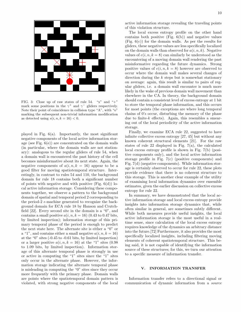
Another interesting example is provided by ECA rule18, which contains domain walls against a seemingly ir-regular background domain. We measured the local val-ues for e(i, n, k = 8) and a(i, n, k = 16) (see Fig. 6(b),Fig. 6(d) and Fig. 6(e)) for the raw states of rule 18 dis-

9

(a)Raw CA (b)e(i, n, k = 8) (c)a(i, n, k = 16) : +ve

(d)a(i, n, k = 16) : −ve (e)t(i, j = 1, n, k = 16) : +ve (f)t(i, j = 1, n, k = 16) : −ve

(g)s(i, n, k = 16) : +ve (h)s(i, n, k = 16) : −ve (i)Collision points

FIG. 2: Local information dynamics in rule 54: (35 time steps displayed for 35 cells, time increases down the page for allCA plots): (b) Local excess entropy, positive values only, (all figures gray-scale with 16 levels) with max. 11.79 bits (black),min. 0.00 bits (white); Local active information: (c) positive values only, max. 1.07 bits (black), min. 0.00 bits (white), (d)negative values only, max. 0.00 bits (white), min. -12.27 bits (black); Local apparent transfer entropy (one cell to the right):(e) positive values only, max. 7.93 bits (black), min. 0.00 bits (white), (f) negative values only, max. 0.00 bits (white), min.-4.04 bits (black); Local separable information: (g) positive values only, max. 8.40 bits (black), min. 0.00 bits (white), (h)negative values only, max. 0.00 bits (white), min. -5.27 bits (black); (i) Positions of s(i, n, k = 16) < 0 marked against thelocal collective transfer entropy profile t(i, n, k = 16).

10

FIG. 3: Close up of raw states of rule 54. “x” and “+”mark some positions in the γ+ and γ− gliders respectively.Note their point of coincidence in collision type “A”, with “o”marking the subsequent non-trivial information modificationas detected using s(i, n, k = 16) < 0.

played in Fig. 6(a). Importantly, the most significantnegative components of the local active information stor-age (see Fig. 6(e)) are concentrated on the domain walls(in particular, where the domain walls are not station-ary): analogous to the regular gliders of rule 54, whena domain wall is encountered the past history of the cellbecomes misinformative about its next state. Again, thenegative components of a(i, n, k = 16) appear to be agood filter for moving spatiotemporal structure. Inter-estingly, in contrast to rules 54 and 110, the backgrounddomain for rule 18 contains both a significant numberof points with negative and with positive (Fig. 6(d)) lo-cal active information storage. Considering these compo-nents together, we observe a pattern to the backgrounddomain of spatial and temporal period 2 corresponding tothe period-2 ǫ-machine generated to recognize the back-ground domain for ECA rule 18 by Hanson and Crutch-field [22]. Every second site in the domain is a “0”, andcontains a small positive a(i, n, k = 16) (0.43 to 0.47 bits,by limited inspection); information storage of this pri-mary temporal phase of the period is enough to predictthe next state here. The alternate site is either a “0” ora “1”, and contains either a small negative a(i, n, k = 16)at the “0” sites (-0.45 to -0.61 bits, by limited inspection)or a larger positive a(i, n, k = 16) at the “1” sites (0.98to 1.09 bits, by limited inspection). Information stor-age of this alternate temporal phase is strongly in useor active in computing the “1” sites since the “1” sitesonly occur in the alternate phase. However, the infor-mation storage indicating the alternate temporal phaseis misleading in computing the “0” sites since they occurmore frequently with the primary phase. Domain wallsare points where the spatiotemporal domain pattern isviolated, with strong negative components of the local

active information storage revealing the traveling pointsof this violation structure.

The local excess entropy profile on the other handcontains both positive (Fig. 6(b)) and negative values(Fig. 6(c)) for the domain walls. As per the results forgliders, these negative values are less specifically localizedon the domain walls than observed for a(i, n, k). Negativevalues of e(i, n, k = 8) can similarly be understood as theencountering of a moving domain wall rendering the pastmisinformative regarding the future dynamics. Strongpositive values of e(i, n, k = 8) however are observed tooccur where the domain wall makes several changes ofdirection during the k steps but is somewhat stationaryon average: again, this result is similar to pairs of reg-ular gliders, i.e. a domain wall encounter is much morelikely in the wake of previous domain wall movement thanelsewhere in the CA. In theory, the background domainshould contain a consistent level of excess entropy at 1 bitto store the temporal phase information, and this occursfor most points (the exceptions are where long temporalchains of 0’s occur, disturbing the memory of the phasedue to finite-k effects). Again, this resembles a smear-ing out of the local periodicity of the active informationstorage.

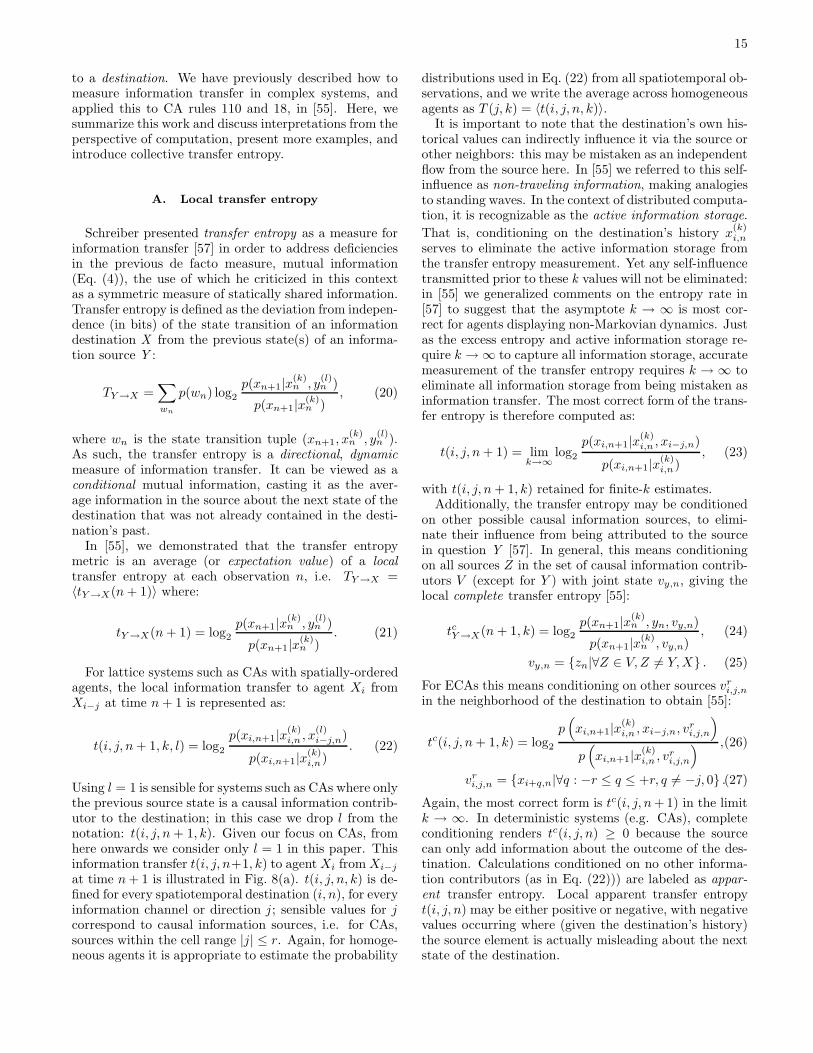
Finally, we examine ECA rule 22, suggested to haveinfinite collective excess entropy [27, 45] but without anyknown coherent structural elements [21]. For the rawstates of rule 22 displayed in Fig. 7(a), the calculatedlocal excess entropy profile is shown in Fig. 7(b) (posi-tive components only), and the local active informationstorage profile in Fig. 7(c) (positive components) andFig. 7(d) (negative components). While information stor-age is certainly observed to occur for rule 22, these plotsprovide evidence that there is no coherent structure tothis storage. This is another clear example of the utilityof examining local information dynamics over ensembleestimates, given the earlier discussion on collective excessentropy for rule 22.

In summary, we have demonstrated that the local ac-tive information storage and local excess entropy provideinsights into information storage dynamics that, whileoften similar in general, are sometimes subtly different.While both measures provide useful insights, the localactive information storage is the most useful in a real-time sense, since calculation of the local excess entropyrequires knowledge of the dynamics an arbitrary distanceinto the future.[72] Furthermore, it also provides the mostspecifically localized insights, including filtering movingelements of coherent spatiotemporal structure. This be-ing said, it is not capable of identifying the informationsource of these structures; for this, we turn our attentionto a specific measure of information transfer.

V. INFORMATION TRANSFER

Information transfer refers to a directional signal orcommunication of dynamic information from a source

11

(a)Raw CA (b)e(i, n, k = 8) (c)a(i, n, k = 16) : +ve

(d)a(i, n, k = 16) : −ve (e)t(i, j = −1, n, k = 16) : +ve (f)t(i, j = −1, n, k = 16) : −ve

(g)hµ(i, n, k = 16) (h)s(i, n, k = 16) : +ve (i)s(i, n, k = 16) : −ve

FIG. 4: Local information dynamics in rule 110: (55 time steps displayed for 55 cells): (b) Local excess entropy, positive valuesonly, max. 10.01 bits (black), min. 0.00 bits (white); Local active information: (c) positive values only, max. 1.22 bits (black),min. 0.00 bits (white), (d) negative values only, max. 0.00 bits (white), min. -9.21 bits (black); Local apparent transfer entropy(one cell to the left): (e) positive values only, max. 10.43 bits (black), min. 0.00 bits (white), (f) negative values only, max.0.00 bits (white), min. -6.01 bits (black); (g) Local temporal entropy rate, max. 10.43 bits (black), min. 0.00 bits (white);Local separable information: (h) positive values only, max. 5.47 bits (black), min. 0.00 bits (white), (i) negative values only,max. 0.00 bits (white), min. -5.20 bits (black).

12

(a)Raw CA (b)e(i, n, k = 5) (c)a(i, n, k = 10) : +ve

(d)a(i, n, k = 10) : −ve (e)t(i, j = 1, n, k = 10) : +ve (f)t(i, j = 3, n, k = 10) : +ve

(g)hµ(i, n, k = 10) (h)s(i, n, k = 10) : +ve (i)s(i, n, k = 10) : −ve

FIG. 5: Local information dynamics in r = 3 rule φpar: (86 time steps displayed for 86 cells): (b) Local excess entropy, positivevalues only, max. 11.76 bits (black), min. 0.00 bits (white); Local active information: (c) positive values only, max. 1.52bits (black), min. 0.00 bits (white), (d) negative values only, max. 0.00 bits (white), min. -9.41 bits (black); Local apparenttransfer entropy: (e) one cell to the right, positive values only, max. 10.45 bits (black), min. 0.00 bits (white), (f) three cell tothe right, positive values only, max. 9.24 bits (black), min. 0.00 bits (white); (g) Local temporal entropy rate, max. 10.92 bits(black), min. 0.00 bits (white); Local separable information: (h) positive values only, max. 29.26 bits (black), min. 0.00 bits(white), (i) negative values only, max. 0.00 bits (white), min. -18.68 bits (black).

13

(a)Raw CA (b)e(i, n, k = 8) : +ve (c)e(i, n, k = 8) : −ve

(d)a(i, n, k = 16) : +ve (e)a(i, n, k = 16) : −ve (f)t(i, j = 1, n, k = 16) : +ve

(g)hµ(i, n, k = 16) (h)s(i, n, k = 16) : +ve (i)s(i, n, k = 16) : −ve

FIG. 6: Local information dynamics in rule 18: (67 time steps displayed for 67 cells): Local excess entropy: (c) negative valuesonly, max. 0.00 bits (black), min. -8.65 bits (black); Local active information: (d) positive values only, max. 1.98 bits (black),min. 0.00 bits (white), (e) negative values only, max. 0.00 bits (white), min. -9.92 bits (black); (f) Local apparent transferentropy (one cell to the right), positive values only, max. 11.90 bits (black), min. 0.00 bits (white); (g) Local temporal entropyrate, max. 11.90 bits (black), min. 0.00 bits (white); Local separable information: (h) positive values only, max. 1.98 bits(black), min. 0.00 bits (white), (i) negative values only, max. 0.00 bits (white), min. -14.37 bits (black).

14

(a)Raw CA (b)e(i, n, k = 8) (c)a(i, n, k = 16) : +ve

(d)a(i, n, k = 16) : −ve (e)t(i, j = 1, n, k = 16) : +ve (f)t(i, j = 1, n, k = 16) : −ve

(g)hµ(i, n, k = 16) (h)s(i, n, k = 16) : +ve (i)s(i, n, k = 16) : −ve

FIG. 7: Local information dynamics in rule 22: (67 time steps displayed for 67 cells): (b) Local excess entropy, positive valuesonly, max. 4.49 bits (black), min. 0.00 bits (white); Local active information: (c) positive values only, max. 1.51 bits (black),min. 0.00 bits (white), (d) negative values only, max. 0.00 bits (white), min. -8.17 bits (black); Local apparent transfer entropy(one cell to the right): (e) positive values only, max. 9.68 bits (black), min. 0.00 bits (white), (f) negative values only, max.0.00 bits (white), min. -7.05 bits (black); (g) Local temporal entropy rate, max. 9.68 bits (black), min. 0.00 bits (white); Localseparable information: (h) positive values only, max. 5.03 bits (black), min. 0.00 bits (white), (i) negative values only, max.0.00 bits (white), min. -14.44 bits (black).

15

to a destination. We have previously described how tomeasure information transfer in complex systems, andapplied this to CA rules 110 and 18, in [55]. Here, wesummarize this work and discuss interpretations from theperspective of computation, present more examples, andintroduce collective transfer entropy.

A. Local transfer entropy

Schreiber presented transfer entropy as a measure forinformation transfer [57] in order to address deficienciesin the previous de facto measure, mutual information(Eq. (4)), the use of which he criticized in this contextas a symmetric measure of statically shared information.Transfer entropy is defined as the deviation from indepen-dence (in bits) of the state transition of an informationdestination X from the previous state(s) of an informa-tion source Y :

TY →X =∑

wn

p(wn) log2

p(xn+1|x(k)n , y

(l)n )

p(xn+1|x(k)n )

, (20)

where wn is the state transition tuple (xn+1, x(k)n , y

(l)n ).

As such, the transfer entropy is a directional, dynamic

measure of information transfer. It can be viewed as aconditional mutual information, casting it as the aver-age information in the source about the next state of thedestination that was not already contained in the desti-nation’s past.

In [55], we demonstrated that the transfer entropymetric is an average (or expectation value) of a local

transfer entropy at each observation n, i.e. TY →X =〈tY →X(n + 1)〉 where:

tY →X(n + 1) = log2

p(xn+1|x(k)n , y

(l)n )

p(xn+1|x(k)n )

. (21)

For lattice systems such as CAs with spatially-orderedagents, the local information transfer to agent Xi fromXi−j at time n + 1 is represented as:

t(i, j, n + 1, k, l) = log2

p(xi,n+1|x(k)i,n , x

(l)i−j,n)

p(xi,n+1|x(k)i,n)

. (22)

Using l = 1 is sensible for systems such as CAs where onlythe previous source state is a causal information contrib-utor to the destination; in this case we drop l from thenotation: t(i, j, n + 1, k). Given our focus on CAs, fromhere onwards we consider only l = 1 in this paper. Thisinformation transfer t(i, j, n+1, k) to agent Xi from Xi−j

at time n + 1 is illustrated in Fig. 8(a). t(i, j, n, k) is de-fined for every spatiotemporal destination (i, n), for everyinformation channel or direction j ; sensible values for jcorrespond to causal information sources, i.e. for CAs,sources within the cell range |j| ≤ r. Again, for homoge-neous agents it is appropriate to estimate the probability

distributions used in Eq. (22) from all spatiotemporal ob-servations, and we write the average across homogeneousagents as T (j, k) = 〈t(i, j, n, k)〉.

It is important to note that the destination’s own his-torical values can indirectly influence it via the source orother neighbors: this may be mistaken as an independentflow from the source here. In [55] we referred to this self-influence as non-traveling information, making analogiesto standing waves. In the context of distributed computa-tion, it is recognizable as the active information storage.

That is, conditioning on the destination’s history x(k)i,n

serves to eliminate the active information storage fromthe transfer entropy measurement. Yet any self-influencetransmitted prior to these k values will not be eliminated:in [55] we generalized comments on the entropy rate in[57] to suggest that the asymptote k → ∞ is most cor-rect for agents displaying non-Markovian dynamics. Justas the excess entropy and active information storage re-quire k → ∞ to capture all information storage, accuratemeasurement of the transfer entropy requires k → ∞ toeliminate all information storage from being mistaken asinformation transfer. The most correct form of the trans-fer entropy is therefore computed as:

t(i, j, n + 1) = limk→∞

log2

p(xi,n+1|x(k)i,n , xi−j,n)

p(xi,n+1|x(k)i,n)

, (23)

with t(i, j, n + 1, k) retained for finite-k estimates.Additionally, the transfer entropy may be conditioned

on other possible causal information sources, to elimi-nate their influence from being attributed to the sourcein question Y [57]. In general, this means conditioningon all sources Z in the set of causal information contrib-utors V (except for Y ) with joint state vy,n, giving thelocal complete transfer entropy [55]:

tcY →X(n + 1, k) = log2

p(xn+1|x(k)n , yn, vy,n)

p(xn+1|x(k)n , vy,n)

, (24)

vy,n = {zn|∀Z ∈ V, Z 6= Y, X} . (25)

For ECAs this means conditioning on other sources vri,j,n

in the neighborhood of the destination to obtain [55]:

tc(i, j, n + 1, k) = log2

p(

xi,n+1|x(k)i,n , xi−j,n, vr

i,j,n

)

p(

xi,n+1|x(k)i,n , vr

i,j,n

) ,(26)

vri,j,n = {xi+q,n|∀q : −r ≤ q ≤ +r, q 6= −j, 0} .(27)

Again, the most correct form is tc(i, j, n + 1) in the limitk → ∞. In deterministic systems (e.g. CAs), completeconditioning renders tc(i, j, n) ≥ 0 because the sourcecan only add information about the outcome of the des-tination. Calculations conditioned on no other informa-tion contributors (as in Eq. (22))) are labeled as appar-ent transfer entropy. Local apparent transfer entropyt(i, j, n) may be either positive or negative, with negativevalues occurring where (given the destination’s history)the source element is actually misleading about the nextstate of the destination.

16

(a)Transfer Entropy (b)Separable Information

FIG. 8: (a) Transfer Entropy t(i, j, n+1, k): information contained in the source cell Xi−j about the next state of the destinationcell Xi at time time n+1 that was not contained in the destination’s past. (b) Separable information s(i, n+1, k): informationgained about the next state of the destination from separately examining each causal information source in the context of thedestination’s past. For ECAs these causal sources are within the cell range r.

B. Total information, entropy rate and collective

information transfer

The total information required to predict the nextstate of any agent i is the local entropy h(i, n + 1),where the entropy is the average of these local values:H(Xi) = 〈h(i, n + 1)〉. Similarly, the local temporal en-

tropy rate hµ(i, n + 1, k) is the information to predictthe next state of agent i given that agent’s past, andthe entropy rate is the average of these local values:Hµ(Xi, k) = 〈hµ(i, n + 1, k)〉. As demonstrated in Ap-pendix A, the local entropy can be considered as the sumof the local active information storage a(i, n + 1, k) andlocal temporal entropy rate:

h(i, n + 1) = a(i, n + 1, k) + hµ(i, n + 1, k). (28)

For deterministic systems (e.g. CAs) there is no intrinsicuncertainty, so the local temporal entropy rate is equalto the local collective transfer entropy (see Appendix A)and represents a collective information transfer: the in-formation about the next state of the destination jointlyadded by the causal information sources that was notcontained in the past of the destination. Also, AppendixA shows that (via a sum of incrementally conditionedmutual information terms) for ECAs we have:

h(i, n + 1) = a(i, n + 1, k) + t(i, j = −1, n + 1, k) +

tc(i, j = 1, n + 1, k), (29)

(and vice-versa in j = 1,−1).Clearly, this total information is not simply a simple

sum of the active information transfer and the appar-ent transfer entropy from each source, nor the sum of

the active information transfer and the complete trans-fer entropy from each source. In earlier work [55], wedemonstrated that the sum of transfer entropies fromeach source (either apparent or complete) formed a use-ful single spatiotemporal filter for emergent structure inCAs, whereas the transfer entropy from each source dis-plays information transfer in one given direction only.Given Eq. (28), we suggest that the local collective trans-fer entropy (or simply the local temporal entropy ratehµ(i, n, k) for deterministic systems) is likely to be a moremeaningful measure and filter for this purpose.

C. Local information transfer results

Local complete and apparent transfer entropy were ap-plied to ECA rules 110 and 18 in [55]. Here we revisitthese and present further examples, focusing on the localapparent transfer entropy: profiles of the positive valuesof t(i, j = 1, n, k = 16) are plotted for rules 54 (Fig. 2(e)),φpar (Fig. 5(e)), 18 (Fig. 6(f)) and 22 (Fig. 7(e)), witht(i, j = −1, n, k = 16) plotted for rule 110 (Fig. 4(e)). Wealso measure the profiles of the local temporal entropyrate hµ(i, n + 1, k) (which is equal to the local collectivetransfer entropy in these deterministic systems) here inFig. 4(g) for rule 110, Fig. 5(g) for φpar , and Fig. 6(g)for rule 18.

Both the local apparent and complete transfer en-tropy highlight particles (including gliders and domainwalls) as strong positive information transfer againstbackground domains. Importantly, the particles are mea-sured as information transfer in their direction of macro-scopic motion, as expected. For example, at the “x”

17

marks in Fig. 3 which denote parts of the right-moving

γ+ gliders, we have p(xi,n+1|x(k=16)i,n , xi−1,n) = 1.00 and

p(xi,n+1|x(k=16)i,n ) = 0.25: there is a strong information

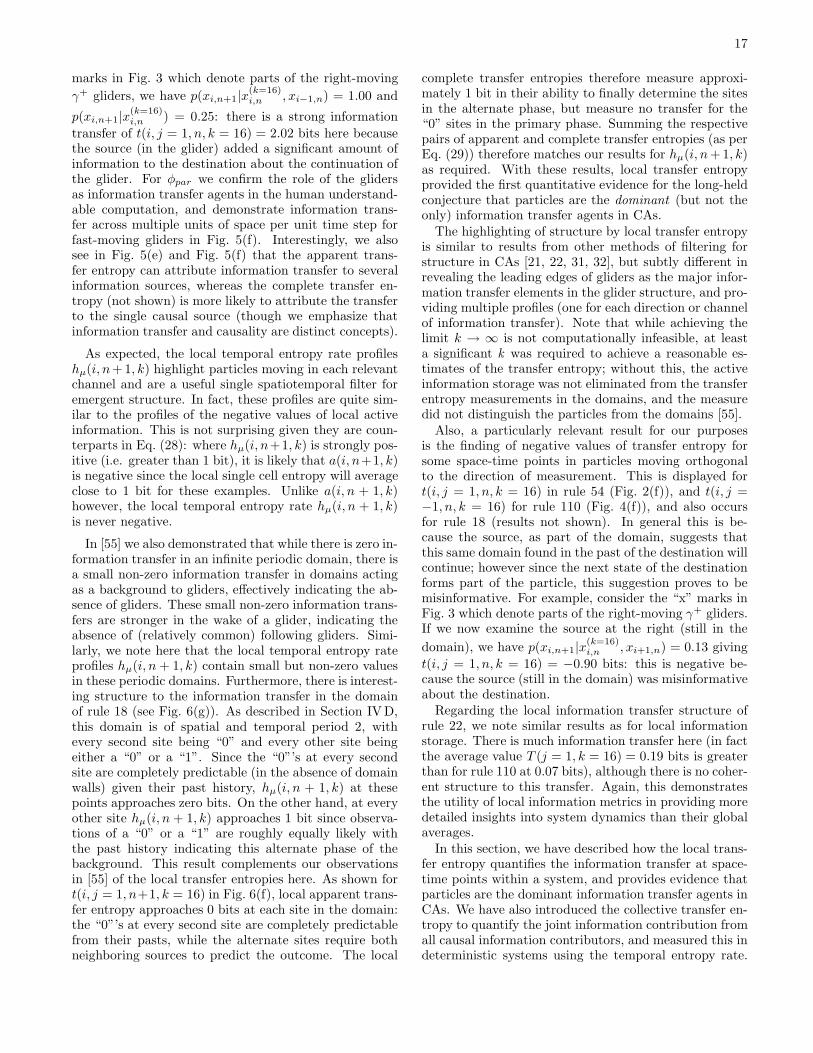
transfer of t(i, j = 1, n, k = 16) = 2.02 bits here becausethe source (in the glider) added a significant amount ofinformation to the destination about the continuation ofthe glider. For φpar we confirm the role of the glidersas information transfer agents in the human understand-able computation, and demonstrate information trans-fer across multiple units of space per unit time step forfast-moving gliders in Fig. 5(f). Interestingly, we alsosee in Fig. 5(e) and Fig. 5(f) that the apparent trans-fer entropy can attribute information transfer to severalinformation sources, whereas the complete transfer en-tropy (not shown) is more likely to attribute the transferto the single causal source (though we emphasize thatinformation transfer and causality are distinct concepts).

As expected, the local temporal entropy rate profileshµ(i, n+1, k) highlight particles moving in each relevantchannel and are a useful single spatiotemporal filter foremergent structure. In fact, these profiles are quite sim-ilar to the profiles of the negative values of local activeinformation. This is not surprising given they are coun-terparts in Eq. (28): where hµ(i, n+1, k) is strongly pos-itive (i.e. greater than 1 bit), it is likely that a(i, n+1, k)is negative since the local single cell entropy will averageclose to 1 bit for these examples. Unlike a(i, n + 1, k)however, the local temporal entropy rate hµ(i, n + 1, k)is never negative.

In [55] we also demonstrated that while there is zero in-formation transfer in an infinite periodic domain, there isa small non-zero information transfer in domains actingas a background to gliders, effectively indicating the ab-sence of gliders. These small non-zero information trans-fers are stronger in the wake of a glider, indicating theabsence of (relatively common) following gliders. Simi-larly, we note here that the local temporal entropy rateprofiles hµ(i, n + 1, k) contain small but non-zero valuesin these periodic domains. Furthermore, there is interest-ing structure to the information transfer in the domainof rule 18 (see Fig. 6(g)). As described in Section IVD,this domain is of spatial and temporal period 2, withevery second site being “0” and every other site beingeither a “0” or a “1”. Since the “0”’s at every secondsite are completely predictable (in the absence of domainwalls) given their past history, hµ(i, n + 1, k) at thesepoints approaches zero bits. On the other hand, at everyother site hµ(i, n + 1, k) approaches 1 bit since observa-tions of a “0” or a “1” are roughly equally likely withthe past history indicating this alternate phase of thebackground. This result complements our observationsin [55] of the local transfer entropies here. As shown fort(i, j = 1, n+1, k = 16) in Fig. 6(f), local apparent trans-fer entropy approaches 0 bits at each site in the domain:the “0”’s at every second site are completely predictablefrom their pasts, while the alternate sites require bothneighboring sources to predict the outcome. The local

complete transfer entropies therefore measure approxi-mately 1 bit in their ability to finally determine the sitesin the alternate phase, but measure no transfer for the“0” sites in the primary phase. Summing the respectivepairs of apparent and complete transfer entropies (as perEq. (29)) therefore matches our results for hµ(i, n + 1, k)as required. With these results, local transfer entropyprovided the first quantitative evidence for the long-heldconjecture that particles are the dominant (but not theonly) information transfer agents in CAs.

The highlighting of structure by local transfer entropyis similar to results from other methods of filtering forstructure in CAs [21, 22, 31, 32], but subtly different inrevealing the leading edges of gliders as the major infor-mation transfer elements in the glider structure, and pro-viding multiple profiles (one for each direction or channelof information transfer). Note that while achieving thelimit k → ∞ is not computationally infeasible, at leasta significant k was required to achieve a reasonable es-timates of the transfer entropy; without this, the activeinformation storage was not eliminated from the transferentropy measurements in the domains, and the measuredid not distinguish the particles from the domains [55].

Also, a particularly relevant result for our purposesis the finding of negative values of transfer entropy forsome space-time points in particles moving orthogonalto the direction of measurement. This is displayed fort(i, j = 1, n, k = 16) in rule 54 (Fig. 2(f)), and t(i, j =−1, n, k = 16) for rule 110 (Fig. 4(f)), and also occursfor rule 18 (results not shown). In general this is be-cause the source, as part of the domain, suggests thatthis same domain found in the past of the destination willcontinue; however since the next state of the destinationforms part of the particle, this suggestion proves to bemisinformative. For example, consider the “x” marks inFig. 3 which denote parts of the right-moving γ+ gliders.If we now examine the source at the right (still in the

domain), we have p(xi,n+1|x(k=16)i,n , xi+1,n) = 0.13 giving

t(i, j = 1, n, k = 16) = −0.90 bits: this is negative be-cause the source (still in the domain) was misinformativeabout the destination.

Regarding the local information transfer structure ofrule 22, we note similar results as for local informationstorage. There is much information transfer here (in factthe average value T (j = 1, k = 16) = 0.19 bits is greaterthan for rule 110 at 0.07 bits), although there is no coher-ent structure to this transfer. Again, this demonstratesthe utility of local information metrics in providing moredetailed insights into system dynamics than their globalaverages.

In this section, we have described how the local trans-fer entropy quantifies the information transfer at space-time points within a system, and provides evidence thatparticles are the dominant information transfer agents inCAs. We have also introduced the collective transfer en-tropy to quantify the joint information contribution fromall causal information contributors, and measured this indeterministic systems using the temporal entropy rate.

18

However, we have not yet separately identified collisionevents in CAs: to complete our exploration of the infor-mation dynamics of computation, we now consider thenature of information modification.

VI. INFORMATION MODIFICATION

Langton interpreted information modification as in-teractions between transmitted and/or stored informa-tion which resulted in a modification of one or the other[3]. CAs provide an illustrative example, where the terminteractions is generally interpreted to mean collisionsof particles (including blinkers as information storage),with the resulting dynamics involving something otherthan the incoming particles continuing unperturbed. Theresulting dynamics could involve zero or more particles(with an annihilation leaving only a background domain),and perhaps even some of the incoming particles. Thenumber of particles resulting from a collision has beenstudied elsewhere [43]. Given the focus on perturbationsin the definition here, it is logical to associate a collisionevent with the modification of transmitted and/or storedinformation, and to see it as an information processingor decision event. Indeed, as an information processingevent the important role of collisions in determining thedynamics of the system is widely acknowledged [43], e.g.in the φpar density classification.

Attempts have previously been made to quantify in-formation modification or processing in a system [14, 16,17]. However, these have either been too specific to al-low portability across system types (e.g. by focusing onthe capability of a system to solve a known problem,or measuring properties related to the particular type ofsystem being examined), focus on general processing asmovement or interpretation of information rather thanspecifically the modification of information, or are notamenable to measuring information modification at localspace-time points within a distributed system. In thissection, we present the separable information as a tool todetect non-trivial information modification events, anddemonstrate it as the first measure to identify collisionsin CAs as such.

A. Local separable information

We begin by considering what it means for a particleto be modified. For the simple case of a glider, a modifi-cation is simply an alteration to the predictable periodicpattern of the glider’s dynamics. At such points, an ob-server would be surprised or misinformed about the nextstate of the glider, having not taken account of the en-tity about to perturb it. This interpretation is a clear re-minder of our earlier comments that local apparent trans-fer entropy t(i, j, n) and local active information storagea(i, n) were negative where the respective informationsources were misinformative about the next state of the

information destination (in the context of the destina-tion’s past for transfer entropy). Local active informationstorage was misinformative at gliders, and local apparenttransfer entropy was misinformative at gliders travelingin the orthogonal direction to the measurement. Thisbeing said, one expects that the local apparent transferentropy measured in the direction of glider motion will bemore informative about its evolution than any misinfor-mation conveyed from other sources. However, where theglider is modified by a collision with another glider, wecan no longer expect the local apparent transfer entropyin its macroscopic direction of motion to remain infor-mative about its evolution. Assuming that the incidentglider is also be perturbed, the local apparent transfer en-tropy in its macroscopic direction of motion will also notbe informative about its evolution at this collision point.We expect the same argument to be true for irregularparticles, or domain walls.

As such, we make the hypothesis that at the spatiotem-poral location of a local information modification event orcollision, separate inspection of each information sourcewill misinform an observer overall about the next state ofthe modified information destination. More specifically,the information sources referred to here are the past his-tory of the destination (via the local active informationstorage) and each other causal information contributor(examined in the context of the past history of the des-tination, via their local apparent transfer entropies).

We quantify the total information gained from separateobservation of the information storage and informationtransfer contributors as the local separable information

sX(n):

sX(n) = aX(n) +∑

Y ∈V,Y 6=X

tY →X(n), (30)

with the subscripts indicating the destination and sourcevariables. Again, the separable information SX denotesthe average SX = 〈sX(n)〉. For CAs, where the causalinformation contributors are homogeneously within theneighborhood r, we write the local separable informationin lattice notation as:

s(i, n) = a(i, n) ++r∑

j=−r,j 6=0

t(i, j, n). (31)

We use s(i, n, k) to represent finite-k estimates, and shows(i, n, k) diagrammatically in Fig. 8(b).[73]

As inferred earlier, we expect the local separable infor-mation to be positive or highly separable where separateobservations of the information contributors are informa-tive overall regarding the next state of the destination.This may be interpreted as a trivial information mod-ification, because information storage and transfer arenot interacting in any significant manner. More impor-tantly, we expect the local separable information to benegative at spatiotemporal points where an informationmodification event or collision takes place. Here, sepa-rate observations are misleading overall because a non-trivial information modification is taking place (i.e. the

19

information storage and transfer are interacting. It isthus clear how we can understand information modifica-tion as the interaction between information storage andinformation transfer.

Importantly, this formulation of non-trivial informa-tion modification aligns with the descriptions of complexsystems as consisting of (a large number of) elements in-teracting in a non-trivial fashion [24], and of emergenceas where “the whole is greater than the sum of its parts”.Here, we quantify the sum of the parts in s(i, n), and “thewhole” refers to examining all information sources to-gether; the whole is greater where all information sourcesmust be examined together in order to receive positive in-formation on the next state of the examined entity. Thatbeing said, there is no quantity representing “the whole”as such, simply the indication that the sources must beexamined together. We emphasize that s(i, n) is not thetotal information an observer needs to predict the stateof the destination; this is measured by the single-site en-tropy h(i, n) (see Section A).

Finally, we introduce the notation S+(k) and S−(k)as the averages of positive and negative local values ofs(i, n, k) in contributing to the average S(k). We havefor example S+(k) = 〈s+(i, n, k)〉, where:

s+(i, n, k) =

{

s(i, n, k) if s(i, n, k) ≥ 00 if s(i, n, k) < 0

, (32)

while S−(k) = 〈s−(i, n, k)〉 is defined in the oppositemanner.

B. Local separable information results

The simple gliders in ECA rule 54 give rise to relativelysimple collisions which we focus on in our discussion here.The positive values of s(i, n, k = 16) for rule 54 are dis-played in Fig. 2(g); notice that these are concentratedin the domain regions and at the stationary gliders (αand β). As expected, these regions are undertaking triv-ial computations only. Fig. 2(h) displays the negativevalues of s(i, n, k = 16), with their positions marked inFig. 2(i). The dominant negative values are clearly con-centrated around the areas of collisions between the glid-ers, including collisions between the traveling gliders only(marked by “A”) and between the traveling gliders andthe stationary gliders (marked by “B”, “C” and “D”).

Collision “A” involves the γ+ and γ− particles inter-acting to produce a β particle (γ+ + γ− → β [43]).The only information modification point highlighted isone time step below the point at which the glidersnaively appear to collide (see close-up of raw states inFig. 3). The periodic pattern in the past of the desti-nation breaks there, however the neighboring sources arestill able to support separate prediction of the state (i.e.a(i, n, k = 16) = −1.09 bits, t(i, j = 1, n, k = 16) = 2.02bits and t(i, j = −1, n, k = 16) = 2.02 bits, givings(i, n, k = 16) = 2.95 bits). This is no longer the case

however where our metric has successfully identified themodification point; there we have a(i, n, k = 16) = −3.00bits, t(i, j = 1, n, k = 16) = 0.91 bits and t(i, j =−1, n, k = 16) = 0.90 bits, with s(i, n, k = 16) = −1.19bits suggesting a non-trivial information modification. Adelay is also observed before the identified informationmodification points of collision types “B” (γ+ +β → γ−,or vice-versa in γ-types), “C” (γ− + α → γ− + α + 2γ+,or vice-versa) and “D” (2γ+ + α + 2γ− → α); possiblythese delays represent a time-lag of information process-ing. Not surprisingly, the results for these other collisiontypes imply that the information modification points areassociated with the creation of new behavior: in “B” and“C” these occur along the newly created γ gliders, andfor “C” and “D” in the new α blinkers.

Importantly, weaker information modification pointscontinue to be identified at every second point along allthe γ+ and γ− particles after the initial collisions (theseare too weak to appear in Fig. 2(h) but can be seen fora similar glider in rule 110 in Fig. 4(i)). This was un-expected from our earlier hypothesis. However, theseevents can be understood as non-trivial computations ofthe continuation of the glider in the absence of a colli-sion; in effect they are virtual collisions between the realglider and the absence of an incident glider. These weakcollision events are more significant in the wake of realcollisions, since incident gliders are relatively more likelyin these areas. Interestingly, this finding is analogous tothe small but non-zero information transfer in periodicdomains indicating the absence of gliders.

We also note that measurements of local independentlyobserved information must be performed with a reason-ably large value of k. Earlier, we observed that for appro-priate measurement of information storage and transferk should be selected to be as large as possible for accu-racy, at least larger than the scale of the period of theregular background domain for filtering purposes. Here,using k < 4 could not distinguish any information mod-ification points clearly from the domains and particles,and even k < 8 could not distinguish all the modifica-tion points (results not shown). Correct quantification ofinformation modification requires satisfactory estimatesof information storage and transfer, and accurate distinc-tion between the two.

We observe similar results in the profile of s(i, n, k =10) for φpar, confirming that the particle collisions hereas non-trivial information modification events, and there-fore completing the evidence for all of the conjecturesabout this human understandable computation.

The results for s(i, n, k = 16) for ECA rule 110 (seeFig. 4(h) and Fig. 4(i)) are also similar to those for rule54. Here, we have collisions “A” and “B” which shownon-trivial information modification points slightly de-layed from the collision in a similar fashion to those forrule 54. We note that collisions between some of themore complex glider structures in rule 110 (not shown)exhibit non-trivial information modification points whichare more difficult to interpret, and which are even more

20

delayed from the initiation of the collision. The largerdelay is perhaps this is a reflection of the more complexgliders requiring more time steps for the processing totake place. An interesting result not seen for rule 54 is acollision where an incident glider is absorbed by a blinker(see label “C”), without any modification to the absorb-ing glider. No information modification is detected forthis absorption event by s(i, n, k = 16): this is as ex-pected because the information storage for the absorbingblinker is sufficient to predict the dynamics at this inter-action.

As a further test of the measure, we examine collisionsbetween the domain walls of rule 18. As displayed inFig. 6(i), the collision between the domain walls is quiteclearly highlighted as the dominant information modifi-cation event for this rule. The initial information modi-fication event is clearly where one would naively identifythe collision point, yet it is followed by two secondaryinformation modification points separated by two timesteps. At the raw states of these three collision points inFig. 6(a), the outer domains have effectively coalesced,however the observer cannot be certain that the new do-main has taken hold at this particular cell until observinga “1” at the alternate phase. As such, information mod-ification events are observed at each point in the newalternate phase until a “1” confirms the outer domainshave joined. This could provide a parallel to the obser-vation of delays in information processing observed ear-lier. Importantly, this result provides evidence that col-lision of irregular particles are information modificationevents, as expected. It is also worth noting that thesecollisions always result in the destruction of the domainwalls (and the inner domain), indicating that our methodcaptures destruction events as well as creation. (This isalso true for the γ+ + γ− + β → ⊘ event in rule 54, notshown). Also, as displayed in Fig. 6(h) and Fig. 6(i),the background domain takes values of s(i, n, k = 16)as either positive or negative with a(i, n, k = 16), sincet(i, j = 1, n, k = 16) and t(i, j = −1, n, k = 16) vanishat these points. This indicates that some minor infor-mation processing is required to compute the “0” sitesin the alternate phase (whereas the “0” sites for everysecond point and the “1”’s in the alternate phase aretrivial computations dominated by information storage).Finally, the domain walls here appear to give rise to onlypositive values of s(i, n, k = 16). This indicates that thedomains walls contain only trivial information modifica-tion, in contrast with the gliders in rule 54 which requireda small amount of non-trivial information processing inorder to compute their continuation. This is perhapsakin to the observation in [21] that the domain walls inrule 146 are largely determined by the dynamics on eitherside, i.e. they are not the result of any interaction per sebut of dominance from a single source at each time step.

We also apply s(i, n, k = 16) to ECA rule 22, as dis-played in Fig. 7(i) and Fig. 7(i). As could be expectedfrom our earlier results, there are many points of bothpositive and negative local separable information here.

The presence of negative values implies the occurance ofnon-trivial information modification, yet there does notappear to be any structure to these profiles. Again, thisaligns well with the lack of coherent structure found us-ing the other measures in this framework and from thelocal statistical complexity profile of rule 22 [21].

Here, we have introduced the local separable informa-tion to quantify information modification at each spa-tiotemporal point in a complex system. Informationmodification events occur where the separable informa-tion is negative, indicating that separate or independentinspection of the causal information sources (in the con-text of the destination’s past) is misleading because ofnon-trivial interaction between these sources. The lo-cal separable information was demonstrated to providethe first quantitative evidence that particle collisions inCAs are the dominant information modification eventstherein. The measure is capable of identifying events in-volving both creation and destruction, and interestinglythe location of an information modification event oftenappears delayed perhaps due to a time-lag in informationprocessing.

VII. IMPORTANCE OF COHERENT

COMPUTATION

Our framework has proven successful in locally iden-tifying the component operations of distributed compu-tation. We now consider whether this framework canprovide any insights into the overall complexity of com-putation. In other words, what can our results say aboutthe difference in the complex computations of rules 110and 54 as compared to rule 22 and others?

We observe that the coherence of local computationalstructure appears to be the most significant differentiatorhere. “Coherence” implies a property of sticking togetheror a logical relationship [58]: in this context we use theterm to describe a logical spatiotemporal relationship be-tween values in local information dynamics profiles. Forexample, the manner in which particles give rise to simi-lar values of local transfer entropy amongst spatiotempo-ral neighbors is coherent. From the spatiotemporal pro-files presented here, we note that rules 54 and 110 exhibitthe largest amount of coherent computational structure,with rule 18 containing a smaller amount of less coher-ent structure. Rules 22 and 30 (results for rule 30 notshown) certainly exhibit all of the elementary functionsof computation, but do not appear to contain any co-herent structure to their computations. This aligns wellwith similar explorations of local information structurefor these rules, e.g. [21]. Using language reminiscent ofLangton’s analysis [3], we suggest that complex systemsexhibit very highly-structured coherent computation incomparison to ordered systems (which exhibit coherencebut minimal structure in a computation dominated byinformation storage) and chaotic systems (whose compu-tations are dominated by rampant information transfer

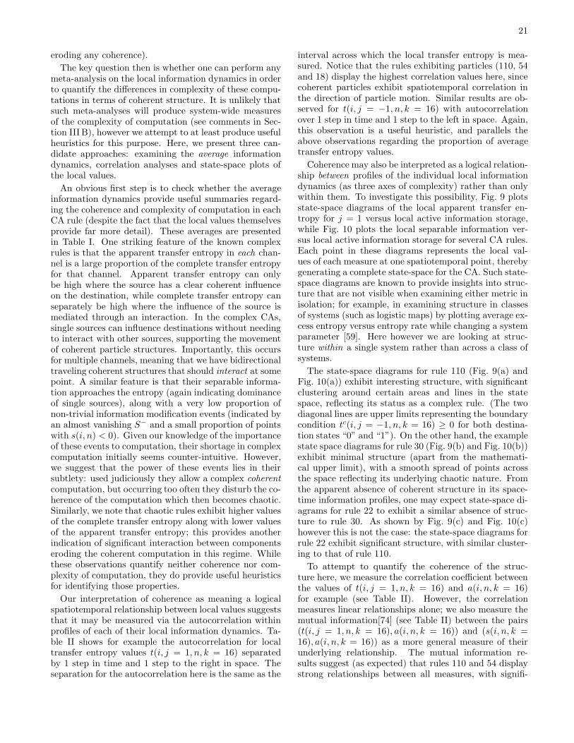
21

eroding any coherence).

The key question then is whether one can perform anymeta-analysis on the local information dynamics in orderto quantify the differences in complexity of these compu-tations in terms of coherent structure. It is unlikely thatsuch meta-analyses will produce system-wide measuresof the complexity of computation (see comments in Sec-tion III B), however we attempt to at least produce usefulheuristics for this purpose. Here, we present three can-didate approaches: examining the average informationdynamics, correlation analyses and state-space plots ofthe local values.

An obvious first step is to check whether the averageinformation dynamics provide useful summaries regard-ing the coherence and complexity of computation in eachCA rule (despite the fact that the local values themselvesprovide far more detail). These averages are presentedin Table I. One striking feature of the known complexrules is that the apparent transfer entropy in each chan-nel is a large proportion of the complete transfer entropyfor that channel. Apparent transfer entropy can onlybe high where the source has a clear coherent influenceon the destination, while complete transfer entropy canseparately be high where the influence of the source ismediated through an interaction. In the complex CAs,single sources can influence destinations without needingto interact with other sources, supporting the movementof coherent particle structures. Importantly, this occursfor multiple channels, meaning that we have bidirectionaltraveling coherent structures that should interact at somepoint. A similar feature is that their separable informa-tion approaches the entropy (again indicating dominanceof single sources), along with a very low proportion ofnon-trivial information modification events (indicated byan almost vanishing S− and a small proportion of pointswith s(i, n) < 0). Given our knowledge of the importanceof these events to computation, their shortage in complexcomputation initially seems counter-intuitive. However,we suggest that the power of these events lies in theirsubtlety: used judiciously they allow a complex coherent

computation, but occurring too often they disturb the co-herence of the computation which then becomes chaotic.Similarly, we note that chaotic rules exhibit higher valuesof the complete transfer entropy along with lower valuesof the apparent transfer entropy; this provides anotherindication of significant interaction between componentseroding the coherent computation in this regime. Whilethese observations quantify neither coherence nor com-plexity of computation, they do provide useful heuristicsfor identifying those properties.

Our interpretation of coherence as meaning a logicalspatiotemporal relationship between local values suggeststhat it may be measured via the autocorrelation withinprofiles of each of their local information dynamics. Ta-ble II shows for example the autocorrelation for localtransfer entropy values t(i, j = 1, n, k = 16) separatedby 1 step in time and 1 step to the right in space. Theseparation for the autocorrelation here is the same as the

interval across which the local transfer entropy is mea-sured. Notice that the rules exhibiting particles (110, 54and 18) display the highest correlation values here, sincecoherent particles exhibit spatiotemporal correlation inthe direction of particle motion. Similar results are ob-served for t(i, j = −1, n, k = 16) with autocorrelationover 1 step in time and 1 step to the left in space. Again,this observation is a useful heuristic, and parallels theabove observations regarding the proportion of averagetransfer entropy values.

Coherence may also be interpreted as a logical relation-ship between profiles of the individual local informationdynamics (as three axes of complexity) rather than onlywithin them. To investigate this possibility, Fig. 9 plotsstate-space diagrams of the local apparent transfer en-tropy for j = 1 versus local active information storage,while Fig. 10 plots the local separable information ver-sus local active information storage for several CA rules.Each point in these diagrams represents the local val-ues of each measure at one spatiotemporal point, therebygenerating a complete state-space for the CA. Such state-space diagrams are known to provide insights into struc-ture that are not visible when examining either metric inisolation; for example, in examining structure in classesof systems (such as logistic maps) by plotting average ex-cess entropy versus entropy rate while changing a systemparameter [59]. Here however we are looking at struc-ture within a single system rather than across a class ofsystems.

The state-space diagrams for rule 110 (Fig. 9(a) andFig. 10(a)) exhibit interesting structure, with significantclustering around certain areas and lines in the statespace, reflecting its status as a complex rule. (The twodiagonal lines are upper limits representing the boundarycondition tc(i, j = −1, n, k = 16) ≥ 0 for both destina-tion states “0” and “1”). On the other hand, the examplestate space diagrams for rule 30 (Fig. 9(b) and Fig. 10(b))exhibit minimal structure (apart from the mathemati-cal upper limit), with a smooth spread of points acrossthe space reflecting its underlying chaotic nature. Fromthe apparent absence of coherent structure in its space-time information profiles, one may expect state-space di-agrams for rule 22 to exhibit a similar absence of struc-ture to rule 30. As shown by Fig. 9(c) and Fig. 10(c)however this is not the case: the state-space diagrams forrule 22 exhibit significant structure, with similar cluster-ing to that of rule 110.

To attempt to quantify the coherence of the struc-ture here, we measure the correlation coefficient betweenthe values of t(i, j = 1, n, k = 16) and a(i, n, k = 16)for example (see Table II). However, the correlationmeasures linear relationships alone; we also measure themutual information[74] (see Table II) between the pairs(t(i, j = 1, n, k = 16), a(i, n, k = 16)) and (s(i, n, k =16), a(i, n, k = 16)) as a more general measure of theirunderlying relationship. The mutual information re-sults suggest (as expected) that rules 110 and 54 displaystrong relationships between all measures, with signifi-

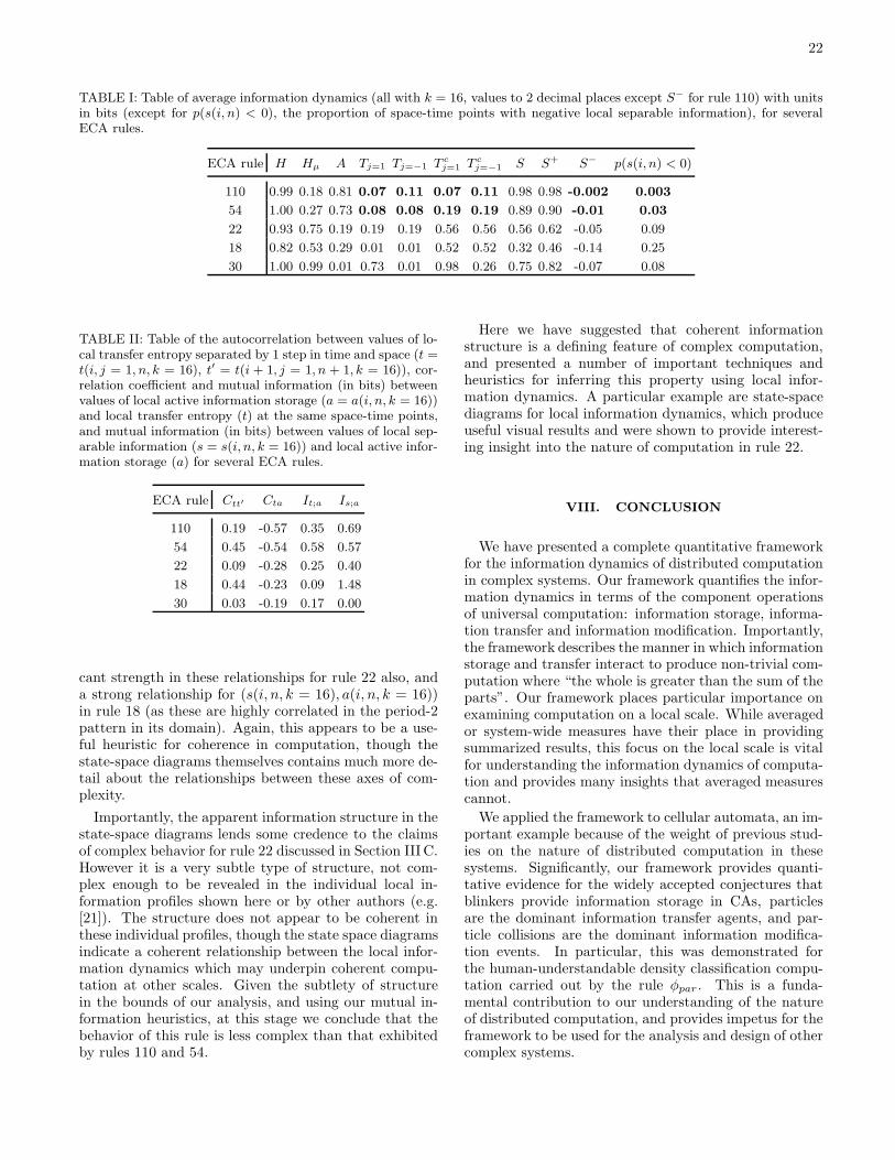
22

TABLE I: Table of average information dynamics (all with k = 16, values to 2 decimal places except S− for rule 110) with unitsin bits (except for p(s(i, n) < 0), the proportion of space-time points with negative local separable information), for severalECA rules.

ECA rule H Hµ A Tj=1 Tj=−1 T cj=1 T c

j=−1 S S+ S− p(s(i, n) < 0)

110 0.99 0.18 0.81 0.07 0.11 0.07 0.11 0.98 0.98 -0.002 0.003

54 1.00 0.27 0.73 0.08 0.08 0.19 0.19 0.89 0.90 -0.01 0.03

22 0.93 0.75 0.19 0.19 0.19 0.56 0.56 0.56 0.62 -0.05 0.09

18 0.82 0.53 0.29 0.01 0.01 0.52 0.52 0.32 0.46 -0.14 0.25

30 1.00 0.99 0.01 0.73 0.01 0.98 0.26 0.75 0.82 -0.07 0.08

TABLE II: Table of the autocorrelation between values of lo-cal transfer entropy separated by 1 step in time and space (t =t(i, j = 1, n, k = 16), t′ = t(i + 1, j = 1, n + 1, k = 16)), cor-relation coefficient and mutual information (in bits) betweenvalues of local active information storage (a = a(i, n, k = 16))and local transfer entropy (t) at the same space-time points,and mutual information (in bits) between values of local sep-arable information (s = s(i, n, k = 16)) and local active infor-mation storage (a) for several ECA rules.

ECA rule Ctt′ Cta It;a Is;a

110 0.19 -0.57 0.35 0.69

54 0.45 -0.54 0.58 0.57

22 0.09 -0.28 0.25 0.40

18 0.44 -0.23 0.09 1.48

30 0.03 -0.19 0.17 0.00

cant strength in these relationships for rule 22 also, anda strong relationship for (s(i, n, k = 16), a(i, n, k = 16))in rule 18 (as these are highly correlated in the period-2pattern in its domain). Again, this appears to be a use-ful heuristic for coherence in computation, though thestate-space diagrams themselves contains much more de-tail about the relationships between these axes of com-plexity.

Importantly, the apparent information structure in thestate-space diagrams lends some credence to the claimsof complex behavior for rule 22 discussed in Section III C.However it is a very subtle type of structure, not com-plex enough to be revealed in the individual local in-formation profiles shown here or by other authors (e.g.[21]). The structure does not appear to be coherent inthese individual profiles, though the state space diagramsindicate a coherent relationship between the local infor-mation dynamics which may underpin coherent compu-tation at other scales. Given the subtlety of structurein the bounds of our analysis, and using our mutual in-formation heuristics, at this stage we conclude that thebehavior of this rule is less complex than that exhibitedby rules 110 and 54.

Here we have suggested that coherent informationstructure is a defining feature of complex computation,and presented a number of important techniques andheuristics for inferring this property using local infor-mation dynamics. A particular example are state-spacediagrams for local information dynamics, which produceuseful visual results and were shown to provide interest-ing insight into the nature of computation in rule 22.

VIII. CONCLUSION

We have presented a complete quantitative frameworkfor the information dynamics of distributed computationin complex systems. Our framework quantifies the infor-mation dynamics in terms of the component operationsof universal computation: information storage, informa-tion transfer and information modification. Importantly,the framework describes the manner in which informationstorage and transfer interact to produce non-trivial com-putation where “the whole is greater than the sum of theparts”. Our framework places particular importance onexamining computation on a local scale. While averagedor system-wide measures have their place in providingsummarized results, this focus on the local scale is vitalfor understanding the information dynamics of computa-tion and provides many insights that averaged measurescannot.

We applied the framework to cellular automata, an im-portant example because of the weight of previous stud-ies on the nature of distributed computation in thesesystems. Significantly, our framework provides quanti-tative evidence for the widely accepted conjectures thatblinkers provide information storage in CAs, particlesare the dominant information transfer agents, and par-ticle collisions are the dominant information modifica-tion events. In particular, this was demonstrated forthe human-understandable density classification compu-tation carried out by the rule φpar . This is a funda-mental contribution to our understanding of the natureof distributed computation, and provides impetus for theframework to be used for the analysis and design of othercomplex systems.

23

(a)110

(b)30

(c)22

FIG. 9: State space diagrams of local transfer entropy (onestep to the right) t(i, j = 1, n, k = 16) versus local activeinformation a(i, n, k = 16) at the same space-time point (i, n)for several ECA rules: (a) 110, (b) 30 and (c) 22.

(a)110

(b)30

(c)22

FIG. 10: State space diagrams of local separable informations(i, n, k = 16) versus local active information a(i, n, k = 16)at the same space-time point (i, n) for several ECA rules: (a)110, (b) 30 and (c) 22.

24

The application to CAs aligned well with other meth-ods of filtering for complex structure in CAs. However,our work is distinct in that it provides several differentviews of the system corresponding to each type of com-putational structure. In particular, the results align wellwith the insights of computational mechanics, providinga strong connection between this field and the local in-formation dynamics of computation.

From our results, we also observed that coherent lo-cal information structure is a defining feature of com-plex distributed computation, and presented a numberof techniques to meta-analyze local information dynam-ics in order to infer coherent complex computation. Here,our framework provides further insight into the natureof computation in rule 22 with respect to the acceptedcomplex rules 54 and 110. Certainly rule 22 exhibitsall of the elementary functions of computation, yet (inline with [21]) there is no apparent coherent structure tothe profiles of its local information dynamics. On theother hand, state space views of the interplay betweenthese local information dynamics reveal otherwise hid-den structure. Our framework is unique in its ability toresolve both of these aspects. We conclude that rule 22exhibits more structure than chaotic rules, yet the sub-tlety of this structure prevent it from being consideredas complex than rules 110 and 54.

The major thrust of our future work is to apply thisframework to other systems, e.g. we are examining com-putation in random Boolean networks as models of generegulatory networks [60] and in modular robotics [61].Given the information-theoretic basis of this framework,it is readily applicable to other systems. Furthermore,we intend to explore the relationship between the infor-mation dynamics description of distributed computationand other perspectives of computation, for example de-scriptions of collective computation (e.g. in the light-conemodel of computational mechanics [21]) and of computa-tional complexity [62].

Acknowledgments

A brief exposition of the local active information andlocal separable information were previously published as[63]. The authors thank Melanie Mitchell for helpful com-ments and suggestions regarding an early version of thismanuscript. The CA diagrams were generated using en-hancements to [64].

APPENDIX A: TOTAL INFORMATION

COMPOSITION

Here, we demonstrate the mathematical arrangementof information storage and transfer for prediction ofthe next state at any given space-time point in thesystem.[75]

First, note that the average information required topredict the state at any spatiotemporal point is simplythe single cell entropy HX (Eq. (1)). We use the mutualinformation expansion of Eq. (5) to express this entropyin terms of the active information storage and entropyrate estimates[76]:

HX′ = IX′;X(k) + HX′|X(k) . (A1)

For convenience, we switch to local notation with thelocal entropy and local temporal entropy rate estimaterepresented as h(n+1) and hµ(n+1, k) = h(xi,n+1|xi+r,n)respectively, and as h(i, n+1) and hµ(i, n+1, k) in locallattice notation:

h(n + 1) = a(n + 1, k) + hµ(n + 1, k), (A2)

h(i, n + 1) = a(i, n + 1, k) + hµ(i, n + 1, k). (A3)

Logically, we can restate this as: the information to pre-dict a given cell site is the amount predictable from itspast (the active memory) plus the remaining uncertaintyafter examining this memory.

We then consider the composition of this remaining un-certainty, tailoring our notation to CAs. In doing so, wealter Eq. (27) to represent a consecutive group of neigh-bors:

vs,fi,n = {xi+q,n|∀q : s ≤ q ≤ f, q 6= 0} . (A4)

We systematically expand the entropy rate estimateterm in Eq. (A3) by incrementally taking account ofthe contribution of each other information source. Asa first step we identify the contribution from sourcei+ r, the local apparent transfer entropy t(i,−r, n+1, k)represented as a local conditional mutual information

m(xi+r,n; xi,n+1|x(k)i,n) (see [55]):

h(i, n + 1) = a(i, n + 1, k) + m(xi+r,n; xi,n+1|x(k)i,n) +

h(xi,n+1|xi+r,n, x(k)i,n). (A5)

The systemic expansion is performed by using Eq. (7)iteratively on the rightmost conditional entropy term toproduce:

h(i, n + 1) = a(i, n + 1, k) ++r∑

j=−r,j 6=0

m(xi−j,n; xi,n+1|v−j+1,ri,n , x

(k)i,n ) +

h(xi,n+1|v−r,ri,n , x

(k)i,n ). (A6)

The sum of incrementally conditioned mutual informa-tion terms is a sum of transfer entropies from each ele-ment, incrementally conditioned on the previously con-sidered sources in the neighborhood. The first such termin Eq. (A5) is an apparent transfer entropy, and the lastterm of the sum in Eq. (A6) is a complete transfer en-tropy. The order in which these causal information con-tributors are removed is arbitrary; the form of the result

25

will be the same. This sum is a collective transfer entropyfrom the set of all causal sources V to the destination:IV ;X′|X(k) , i.e. the average information about the nextstate of the destination jointly added by the causal infor-mation sources that was not contained in the past of thedestination. In local lattice notation, we have the local

collective transfer entropy t(i, n + 1, k):

t(i, n + 1, k) =

+r∑

j=−r

m(xi+j,n; xi,n+1|v−r,j−1i,n , x

(k)i,n).(A7)

= log2

p(

xi,n+1|x(k)i,n , v−r,r

i,n

)

p(

xi,n+1|x(k)i,n

) (A8)

As before, t(i, n + 1) represents the most correct form inthe limit k → ∞.

Also, we note that the final term in Eq. (A6) is the re-maining local intrinsic uncertainty in the destination af-ter its past and all causal information contributors havebeen considered; we label this as u(i, n + 1) (noting thatit is independent of k). As such, Eq. (A6) logically dis-plays the information to predict the destination at any

space-time point as the sum of the amount predictablefrom its past (active information storage), the amountthen collectively predictable from its causal contributors(collective transfer entropy), and remaining intrinsic un-certainty:

h(i, n + 1) = a(i, n + 1, k) + t(i, n + 1, k) +

u(i, n + 1). (A9)

In a deterministic system, note that there is no remainingintrinsic uncertainty u(i, n + 1). As such, for determin-istic systems (such as CAs) the temporal entropy ratehµ(i, n + 1, k) is equal to the collective transfer entropyt(i, n + 1, k).

As an example, the total information to predict thenext state of any destination in an ECA can be repre-sented as:

h(i, n + 1) = a(i, n + 1, k) + t(i, j = −1, n + 1, k) +

tc(i, j = 1, n + 1, k), (A10)

or vice-versa in j = −1, 1.

[1] M. Mitchell, in Non-Standard Computation, edited byT. Gramss, S. Bornholdt, M. Gross, M. Mitchell, andT. Pellizzari (VCH Verlagsgesellschaft, Weinheim, 1998),pp. 95–140.

[2] M. Mitchell, in 20th Annual Conference of the CognitiveScience Society (Cogsci98), edited by M. A. Gernsbacherand S. J. Derry (Madison, Wisconsin, 1998), pp. 710–715.

[3] C. G. Langton, Physica D 42, 12 (1990).[4] S. Wolfram, Physica D 10, 1 (1984).[5] J. L. Casti, in Beyond belief: randomness, prediction and

explanation in science, edited by J. L. Casti and A. Kar-lqvist (CRC Press, Boca Raton, 1991), pp. 280–327.

[6] M. Prokopenko, V. Gerasimov, and I. Tanev, in NinthInternational Conference on the Simulation of AdaptiveBehavior (SAB’06), edited by S. Nolfi, G. Baldassarre,R. Calabretta, J. Hallam, D. Marocco, J.-A. Meyer, andD. Parisi (Springer Verlag, Rome, 2006), vol. 4095 of Lec-ture Notes in Artificial Intelligence, pp. 548–559.

[7] K. I. Goh and A. L. Barabasi, Europhysics Letters 81,48002 (2008).

[8] R. Morgado, M. Ciesla, L. Longa, and F. A. Oliveira,Europhysics Letters 79, 10002 (2007).

[9] J. A. Brown and J. A. Tuszynski, Ferroelectrics 220,141156 (1999).

[10] J. Pahle, A. K. Green, C. J. Dixon, and U. Kummer,BMC Bioinformatics 9, 139 (2008).

[11] I. Couzin, R. James, D. Croft, and J. Krause, in FishCognition and Behavior, edited by B. C., K. Laland, andJ. Krause (Blackwell Publishing, 2006), Fish and AquaticResources, pp. 166–185.

[12] A. S. Klyubin, D. Polani, and C. L. Nehaniv, in 8th Euro-pean Conference on Artificial Life (ECAL 2005), editedby M. S. Capcarrere, A. A. Freitas, P. J. Bentley, C. G.Johnson, and J. Timmis (Springer Berlin / Heidelberg,

Kent, UK, 2005), vol. 3630 of Lecture Notes in ComputerScience, pp. 744–753.

[13] M. Lungarella and O. Sporns, PLoS Computational Bi-ology 2, e144 (2006).

[14] O. Kinouchi and M. Copelli, Nature Physics 2, 348(2006).

[15] J. J. Atick, Network: Computation in Neural Systems 3,213 (1992).

[16] M. A. Sanchez-Montanes and F. J. Corbacho, in Pro-ceedings of the International Conference on ArtificialNeural Networks (ICANN 2002), Madrid, Spain, editedby J. Dorronsoro (Springer-Verlag, Berlin/Heidelberg,2002), vol. 2415 of Lecture Notes in Computer Science,pp. 141–141.

[17] T. Yamada and K. Aihara, in IEEE Symposium onEmerging Technologies and Factory Automation (ETFA’94) (IEEE, Tokyo, 1994), pp. 239–244.

[18] M. H. Jakubowski, K. Steiglitz, and R. Squier, Phys.Rev. E 56, 7267 (1997).

[19] A. Adamatzky, ed., Collision-Based Computing(Springer-Verlag, Berlin, 2002).

[20] D. E. Edmundson and R. H. Enns, Opt. Lett. 18, 1609(1993).

[21] C. R. Shalizi, R. Haslinger, J.-B. Rouquier, K. L.Klinkner, and C. Moore, Phys. Rev. E 73, 036104 (2006).

[22] J. E. Hanson and J. P. Crutchfield, J. Stat. Phys. 66,1415 (1992).

[23] J. Von Neumann, Theory of self-reproducing automata(University of Illinois Press, Urbana, 1966), edited andcompleted by Arthur W. Burks.

[24] M. Prokopenko, F. Boschetti, and A. J. Ryan (2008),Unpublished.

[25] D. J. MacKay, Information Theory, Inference, andLearning Algorithms (Cambridge University Press, Cam-

26

bridge, 2003).[26] J. P. Crutchfield and D. P. Feldman, Chaos 13, 25 (2003).[27] P. Grassberger, International Journal of Theoretical

Physics 25, 907 (1986).[28] W. Bialek, I. Nemenman, and N. Tishby, Physica A 302,

89 (2001).[29] S. Wolfram, A New Kind of Science (Wolfram Media,

Champaign, IL, USA, 2002).[30] L. Gray, Notices of the American Mathematical Society

50, 200 (2003).[31] A. Wuensche, Complexity 4, 47 (1999).[32] T. Helvik, K. Lindgren, and M. G. Nordahl, in Inter-

national Conference on Cellular Automata for Researchand Industry, edited by P. M. Sloot, B. Chopard, andA. G. Hoekstra (Springer, Berlin/Heidelberg, Amster-dam, 2004), vol. 3305 of Lecture Notes in Computer Sci-ence, pp. 121–130.

[33] S. Wolfram, Nature 311, 419 (1984).[34] J. H. Conway, in Winning ways for your mathematical

plays, edited by E. Berlekamp, J. H. Conway, and R. Guy(Academic Press, New York, 1982), vol. 2, ch. 25, pp.927–962.

[35] M. Cook, Comp. Sys. 15, 1 (2004).[36] K. Lindgren and M. G. Nordahl, Comp. Sys. 4, 299

(1990).[37] M. H. Jakubowski, K. Steiglitz, and R. K. Squier,

Multiple-Valued Logic 6, 439 (2001).[38] D. Eppstein, in More Games of No Chance, edited by

R. J. Nowakowski (Cambridge Univ. Press, 2002), vol. 42of MSRI Publications, pp. 433–453.

[39] M. Mitchell, J. P. Crutchfield, and P. T. Hraber, PhysicaD 75, 361 (1994).

[40] M. Mitchell, J. P. Crutchfield, and R. Das, in First Inter-national Conference on Evolutionary Computation andIts Applications, edited by E. D. Goodman, W. Punch,and V. Uskov (Russian Academy of Sciences, Russia,Moscow, 1996).

[41] N. Boccara, J. Nasser, and M. Roger, Phys. Rev. A 44,866 (1991).

[42] G. J. Martinez, A. Adamatzky, and H. V. McIntosh,Chaos, Solitons and Fractals 28, 100 (2006).

[43] W. Hordijk, C. R. Shalizi, and J. P. Crutchfield, PhysicaD 154, 240 (2001).

[44] S. Wolfram, Comm. Math. Phys. 96, 15 (1984).[45] P. Grassberger, J. Stat. Phys. 45, 27 (1986).[46] H. V. McIntosh, Linear Cellular Automata (Universidad

Autonoma de Puebla, Puebla, Mexico, 1990).[47] R. Badii and A. Politi, Phys. Rev. Lett. 78, 444 (1997).[48] A. Lafusa and T. Bossomaier, in The 2005 IEEE

Congress on Evolutionary Computation (IEEE Press,Edinburgh, 2005), vol. 1, pp. 844–849.

[49] H. Gutowitz and C. Domain, Physica D 103, 155 (1997).[50] P. Grassberger, in Theory and Applications of Cellular

Automata, edited by S. Wolfram (World Scientific Pub-lishing Co. Ltd., Singapore, 1986).

[51] K. Lindgren and M. G. Nordahl, Comp. Sys. 2, 409(1988).

[52] D. P. Feldman and J. P. Crutchfield, Phys. Rev. E 67,051104 (2003).

[53] A. S. Klyubin, D. Polani, and C. L. Nehaniv, in Proceed-ings of the Ninth International Conference on the Simula-tion and Synthesis of Living Systems (ALife IX), Boston,edited by J. Pollack, M. Bedau, P. Husbands, T. Ikegami,and R. A. Watson (MIT Press, 2004), pp. 563–568.

[54] C. R. Shalizi, Ph.D. thesis, University of Wisconsin-Madison (2001).

[55] J. T. Lizier, M. Prokopenko, and A. Y. Zomaya, Phys.Rev. E 77, 026110 (2008).

[56] J. E. Hanson and J. P. Crutchfield, Physica D 103, 169(1997).

[57] T. Schreiber, Phys. Rev. Lett. 85, 461 (2000).[58] Oxford English Dictionary (2008), accessed 8/5/2008,

URL http://www.oed.com/.[59] D. P. Feldman, C. S. McTague, and J. P. Crutchfield,

The organization of intrinsic computation: Complexity-entropy diagrams and the diversity of natural infor-mation processing (2008), arXiv:0806.4789v1 [nlin.CD],URL http://arxiv.org/abs/0806.4789.

[60] J. T. Lizier, M. Prokopenko, and A. Y. Zomaya, in Pro-ceedings of the Eleventh International Conference on theSimulation and Synthesis of Living Systems (ALife XI),Winchester, UK, edited by S. Bullock, J. Noble, R. Wat-son, and M. A. Bedau (MIT Press, Cambridge, MA,2008), pp. 374–381.

[61] J. T. Lizier, M. Prokopenko, I. Tanev, and A. Y. Zomaya,in Proceedings of the Eleventh International Conferenceon the Simulation and Synthesis of Living Systems (ALifeXI), Winchester, UK, edited by S. Bullock, J. Noble,R. Watson, and M. A. Bedau (MIT Press, Cambridge,MA, 2008), pp. 366–373.

[62] J. P. Crutchfield, Physica D 75, 11 (1994).[63] J. T. Lizier, M. Prokopenko, and A. Y. Zomaya, in Ad-

vances in Artificial Life - 9th European Conference onArtificial Life (ECAL 2007), Lisbon, Portugal, edited byF. Almeida e Costa, L. M. Rocha, E. Costa, I. Harvey,and A. Coutinho (Springer, Berlin / Heidelberg, 2007),vol. 4648 of Lecture Notes in Artificial Intelligence, pp.895–904.

[64] M. Wojtowicz, Java cellebrationv.1.50 (2002), online Software, URLhttp://psoup.math.wisc.edu/mcell/mjcell/mjcell.html.

[65] A. Clauset, C. R. Shalizi, and M. E. J.Newman, Power-law distributions in empir-ical data (2007), arXiv:0706.1062v1, URLhttp://arxiv.org/abs/0706.1062v1 .

[66] C. D. Manning and H. Schutze, Foundations of Statisti-cal Natural Language Processing (MIT Press, Cambridge,MA, USA, 1999).

[67] N. Ludtke, S. Panzeri, M. Brown, D. S. Broomhead,J. Knowles, M. A. Montemurro, and D. B. Kell, Jour-nal of The Royal Society Interface (2007).

[68] H. Kantz and T. Schreiber, Nonlinear Time Series Analy-sis (Cambridge University Press, Cambridge, MA, 1997).

[69] HµX(k) here is equivalent to hµ(k + 1) in [26].[70] In doing so, one should use proper quantitative tech-

niques for establishing the presence or otherwise ofpower-laws, similar to [65] but tailored to study mea-surements of general functions rather than distributionsonly.

[71] This is as per Shalizi’s original formulation of the localexcess entropy in [54], however our presentation is fora single time-series rather than the light-cone formula-tion used there. For a detailed description on why suchaverage information-theoretical measures are the expec-tation value of local measures, and why the local mea-sure can simply be taken as the log term within the av-erages measure, the reader is referred to the presenta-tion of local transfer entropy in [55]. Also note that “lo-

27

cal” information-theoretic measures are known as “point-wise” measures elsewhere [66].

[72] Calculation of e(i, n, k) using local block entropies anal-ogous to Eq. (12) would also require block entropies tobe taken into the future to compute the same local in-formation storage values. Without taking account of thedynamics into the future, we will not measure the in-formation storage that will be used in the future of theprocess, but the information storage that is likely to beused in the future.

[73] The separable information has parallels to the sum of“first order terms” (the apparent contribution of eachsource without considering interactions) in the total in-formation of a destination in [67]. The local separableinformation however is distinguished in considering thecontributions in the context of the destination’s past, andevaluating these on a local scale – both features are crit-

ical for an understanding of distributed computation.[74] The mutual information is measured over 200 000 sample

points via kernel estimation of the underlying entropies[68], using a step kernel with precision r = 0.3 and max-imum distance norms.

[75] Similarly motivated is the decomposition of the totalinformation for a destination presented in [67]. Thatapproach however decomposes the total information interms of a sum of mutual information terms of increas-ing size, rather than incrementally conditioned mutualinformation terms. Our presentation in the context of thedestination’s history, and using local terms, is critical foran understanding of computation.

[76] These equations are correct not only in the limit k → ∞

but for estimates with any value of k.