long-term evolution of orbits about a precessing...
TRANSCRIPT
Celestial Mech Dyn Astr (2007) 99:261–292DOI 10.1007/s10569-007-9099-0
ORIGINAL ARTICLE
Long-term evolution of orbits about a precessing oblateplanet: 3. A semianalytical and a purely numericalapproach
Pini Gurfil · Valéry Lainey · Michael Efroimsky
Received: 12 January 2006 / Revised: 31 July 2007 / Accepted: 14 September 2007 /Published online: 21 November 2007© Springer Science+Business Media B.V 2007
Abstract Construction of an accurate theory of orbits about a precessing and nutating oblateplanet, in terms of osculating elements defined in a frame associated with the equator of date,was started in Efroimsky and Goldreich (2004) and Efroimsky (2004, 2005, 2006a, b). Herewe continue this line of research by combining that analytical machinery with numericaltools. Our model includes three factors: the J2 of the planet, its nonuniform equinoctial pre-cession described by the Colombo formalism, and the gravitational pull of the Sun. Thissemianalytical and seminumerical theory, based on the Lagrange planetary equations forthe Keplerian elements, is then applied to Deimos on very long time scales (up to 1 billionyears). In parallel with the said semianalytical theory for the Keplerian elements definedin the co-precessing equatorial frame, we have also carried out a completely independent,purely numerical, integration in a quasi-inertial Cartesian frame. The results agree to withinfractions of a percent, thus demonstrating the applicability of our semianalytical model overlong timescales. Another goal of this work was to make an independent check of whetherthe equinoctial-precession variations predicted for a rigid Mars by the Colombo model could
We use the term “precession” in its general meaning, which includes any change of the instantaneous spinaxis. So generally defined precession embraces the entire spectrum of spin-axis variations—from the polarwander and nutations through the Chandler wobble through the equinoctial precession.
P. GurfilFaculty of Aerospace Engineering, Technion, Haifa 32000, Israele-mail: [email protected]
V. LaineyIMCCE/Observatoire de Paris, UMR 8028 du CNRS, 77 Avenue Denfert-Rochereau,Paris 75014, Francee-mail: [email protected]
V. LaineyObservatoire Royal de Belgique, Avenue Circulaire 3, Brussels 1180, Belgium
M. Efroimsky (B)US Naval Observatory, Washington, DC 20392, USAe-mail: [email protected]
123
262 P. Gurfil et al.
have been sufficient to repel its moons away from the equator. An answer to this question, incombination with our knowledge of the current position of Phobos and Deimos, will help usto understand whether the Martian obliquity could have undergone the large changes ensuingfrom the said model (Ward 1973; Touma and Wisdom 1993, 1994; Laskar and Robutel 1993),or whether the changes ought to have been less intensive (Bills 2006; Paige et al. 2007). It hasturned out that, for low initial inclinations, the orbit inclination reckoned from the precess-ing equator of date is subject only to small variations. This is an extension, to non-uniformequinoctial precession given by the Colombo model, of an old result obtained by Goldreich(1965) for the case of uniform precession and a low initial inclination. However, near-polarinitial inclinations may exhibit considerable variations for up to ±10 deg in magnitude. Thisresult is accentuated when the obliquity is large. Nevertheless, the analysis confirms that anoblate planet can, indeed, afford large variations of the equinoctial precession over hundredsof millions of years, without repelling its near-equatorial satellites away from the equator ofdate: the satellite inclination oscillates but does not show a secular increase. Nor does it showsecular decrease, a fact that is relevant to the discussion of the possibility of high-inclinationcapture of Phobos and Deimos.
Keywords Orbital elements · Osculating elements · Mars · Natural satellites ·Natural satellites’ orbits · Deimos · Equinoctial precession · The Goldreich lock
1 Introduction
1.1 Statement of purpose
The goal of this paper is to explore, by two very different methods, inclination variations of asolar-gravity-perturbed satellite orbiting an oblate planet subject to nonuniform equinoctialprecession. This nonuniformity of precession is caused by the presence of the other planets.Their gravitational pull entails precession of the circumsolar orbit of our planet; this entailsvariations of the solar torque acting on it; these torque variations make the planet’s equinoctialprecession nonuniform; and this nonuniformity, in its turn, influences the behaviour of theplanet’s satellites. This influence is feeble, and we trace with a high accuracy whether it results,over aeons, in purely periodic changes in inclination or can accumulate to secular changes.
This work is but a small part of a larger project whose eventual goal is to build up acomprehensive tool for computation of long-term orbital evolution of satellites. Building thistool, block by block, we are beginning with only three components—the planet’s oblateness,the direct pull of the Sun on the satellite, and the planet’s precession. These phenomenabare a marked effect on the evolution of the orbit. In our subsequent publications, we shallincorporate more effects into our model—the triaxiality, and the bodily tides.
1.2 Motivation
One motivation for this work stems from our intention to carry out an independent checkof whether the equinoctial-precession changes predicted for a rigid Mars by the Colombomodel could have been sufficient to repel its moons away from the equator. An answer to thisquestion, in combination with our knowledge of the current position of Phobos and Deimos,will help us to understand whether the Martian obliquity variations could indeed have under-gone the large variations resulting from the Colombo model, or whether the actual variationsought to have smaller magnitude. Such a check is desirable because the current, Colombo-model-based theory of equinoctial precession (Ward 1973; Touma and Wisdom 1993, 1994;
123
Long-term evolution of orbits 263
Laskar and Robutel 1993), incorporates several approximations. First, the Colombo equa-tion is derived under the assertion that the planet is rigid and is always in its principal spinstate, the angular-momentum vector staying parallel to the angular-velocity one. Second, thisdescription, being only a model, ignores the possibility of planetary catastrophes that mighthave altered the planet’s spin mode. Third, this description ignores that sometimes even weakdissipation (caused, for example, by tides) may be sufficient to quell chaos and regularisethe motion, which may be the case of Mars (Bills 2006). Fourth, it still remains a matter ofcontroversy as to whether the observed pattern of small craters on Mars confirms (Hartmann2007) or disproves (Paige et al. 2007) the strong climatic variations predicted in Ward (1974,1979). All this motivates us to come up with a test based on the necessity to reconcile thevariations of spin with the present near-equatorial positions of Phobos and Deimos. The factthat both moons found themselves on near-equatorial orbits, in all likelihood, billions ofyears ago,1 and that both are currently located within less than 2 degrees from the equator, issurely more than a mere coincidence. An elegant but sketchy calculation by Goldreich (1965)demonstrated that the orbits of initially near-equatorial satellites remain close to the equatorof date for as long as some simplifying assumptions remain valid. As explained in Efroimsky(2004, 2005), these assumptions are valid over time scales not exceeding 100 million years,while at longer times a more careful analysis is required. Its goal will be to explore the limitsfor the possible secular drift of the satellite orbits away from the evolving equator of date.Through comparison of these limits with the present location of the Martian satellites, weshall be able to impose restrictions upon the long-term spin variations of Mars. If, however, itturns out that near-equatorial satellites can, in the face of large equinoctial-precession varia-tions, remain for billions of years close to the moving equator of date, then we shall admit thatMars’ equator could indeed have precessed through billions of years in the manner predictedby the Colombo approximation.
The second motivation for our study comes from the ongoing discussion of whether theMartian satellites might have been captured at high inclinations, their orbits having graduallyapproached the equator afterwards. While a comprehensive check of this hypothesis will needa more detailed model—one that will include Mars’ triaxiality, the tidal forces (Lainey et al.2008), and perhaps other perturbations—the first, rough sketch of this test can be carried outwith only J2, the Sun, and the equinoctial precession taken into account. We perform such arough check for a hypothetical satellite that has all the parameters of Deimos, except that itsinitial inclination is 89.
1 Phobos and Deimos give every appearance of being captured asteroids of the carbonaceous chondritic type,with cratered surfaces older than ∼109 years (Veverka 1977; Pang et al. 1978; Pollack et al. 1979; Tolson et al.1978). If they were captured by gas drag (Burns 1972, 1978), this must have occurred early in the history of thesolar system while the gas disk was substantial enough. Kilgore, Burns, and Pollack (1978) have demonstratednumerically that a gas envelope extending to about ten Martian radii, with a density of 5 × 10⁻⁵ g/cm3 at theMartian surface, could have been capable of capturing satellites of radii about 10 km. At that stage of planetaryformation, the spin of the forming planet would be perpendicular to the planet’s orbit about the Sun—i.e., theobliquity would be small and the gas disk would be nearly coplanar with the planetary orbit. Energetically, acapture would likely be equatorial. This is most easily seen in the context of the restricted three-body problem.The surfaces of zero velocity constrain any reasonable capture to occur from directions near the inner andouter collinear Lagrange points (Szebehely 1967; Murison 1988), which lie in the equatorial plane. Also, asomewhat inclined capture would quickly be equatorialised by the gas disk. If the capture inclination is toohigh, the orbital energy is then too high to allow a long enough temporary capture, and the object wouldhence not encounter enough drag over a long enough time to effect a permanent capture (Murison 1988).Thus, Phobos and Deimos were likely (in as much as we can even use that term) to have been captured intonear-equatorial orbits.
123
264 P. Gurfil et al.
1.3 Mathematical tools
The first steps toward the analytical theory of orbits about a precessing and nutating Earth wereundertaken almost half a century ago by Brouwer (1959), Proskurin and Batrakov (1960),and Kozai (1960). The problem was considered, in application to the Martian satellites, byGoldreich (1965) and, in regard to a circumlunar orbiter, by Brumberg et al. (1971). Thelatter two publications addressed the dynamics as seen in a non-inertial frame co-precessingwith the planet’s equator of date. The analysis was carried out in terms of the so-called“contact” Kepler elements, i.e., in terms of the Kepler elements satisfying a condition differ-ent from that of osculation. Modeling of perturbed trajectories by sequences of instantaneousellipses (or hyperbolae) parameterised with such elements is sometimes very convenientmathematically (Efroimsky 2006c). However, the physical interpretation of such solutionsis problematic, because instantaneous conics defined by nonosculating elements are non-tangent to the trajectory. Though over restricted time scales the secular parts of the contactelements may well approximate the secular parts of their osculating counterparts (Efroimsky2004, 2005), the cleavage between them may grow at longer time scales. This is the reasonwhy a practically applicable treatment of the problem must be performed in the language ofosculating variables.
1.4 The plan
The analytical theory of orbits about a precessing oblate primary, in terms of the Kepler ele-ments defined in a co-precessing (i.e., related to the equator of date) frame, was formulated inEfroimsky (2006a, b) where the planetary equations were approximated by neglecting somehigh-order terms and averaging the others. This way, from the exact equations for osculatingelements, approximate equations for their secular parts were obtained. We shall borrow thoseaveraged Lagrange-type planetary equations, shall incorporate into them the pull of the Sun,and shall numerically explore their solutions. This will give us a method that will be semi-analytical and seminumerical. We shall then apply it to a particular setting—evolution of aMartian satellite and its reaction to the long-term variations of the spin state of Mars. Ourgoal will be to explore whether the spin-axis variations predicted for a rigid Mars permit itssatellites to remain close to the equator of date for hundreds of millions through billions ofyears. In case the answer to this question turns out to be negative, it will compel us to seeknonrigidity-caused restrictions upon the spin variations. Otherwise, the calculations of therigid-Mars inclination variations will remain in force (and so will the subsequent calculationsof Mars obliquity variations); this way, the theory of Ward (1973, 1974, 1979, 1982), Toumaand Wisdom (1993, 1994), and Laskar and Robutel (1993) will get a model-independentconfirmation.
2 Semianalytical treatment of the problem
To understand the evolution of a satellite orbit about a precessing planet, it is natural to modelit with elements defined in a coordinate system associated with the equator of date, i.e., ina frame co-precessing (but not co-rotating) with the planet. A transition from an inertialframe to the co-precessing one is a perturbation that depends not only upon the instantaneousposition but also upon the instantaneous velocity of the satellite. It has been demonstratedby Efroimsky and Goldreich (2004) that such perturbations enter the planetary equationsin a nontrivial way: not only do they alter the disturbing function (which is the negative
123
Long-term evolution of orbits 265
Hamiltonian perturbation) but also they endow the equations with several extra terms that arenot parts of the disturbing function. Some of these nontrivial terms are linear in the planet’sprecession rate µ, some are quadratic in it; the rest are linear in its time derivative µ. Theinertial-forces-caused addition to the disturbing function (i.e., to the negative Hamiltonianperturbation) consists of a term linear and a term quadratic in µ. (See formulae (53–54)in Efroimsky (2004, 2005) or formulae (1) and (6) in Efroimsky (2006a, b).) The essenceof approximation elaborated in Ibid. was to neglect the quadratic terms and to substitutethe terms linear in µ and µ with their secular parts calculated with precision up to e3,inclusively.
2.1 Equations for the secular parts of osculating elements defined in a co-precessingreference frame
We shall begin with five Lagrange-type planetary equations for the secular parts of the orbitalelements defined in a frame co-precessing with the equator of date. These equations, derivedin Efroimsky (2004, 2005), have the following form:
da
dt= −2
µ⊥n
a(1 − e2)1/2
, (1)
de
dt= 5
2
µ⊥n
e(1 − e2)1/2
, (2)
dω
dt= 3
2
n J2(1 − e2
)2
(ρe
a
)2(
5
2cos2 i − 1
2
)− µ⊥ + µn cot i
− cos i
na2(1 − e2)1/2 sin i
⟨µ
(−f × ∂f
∂i
)⟩, (3)
di
dt= −µ1 cos − µ2 sin + cos i
na2(1 − e2)1/2 sin i
⟨µ
(−f × ∂f
∂ω
)⟩
− 1
na2 (1 − e2)1/2 sin i
⟨µ
(−f × ∂f
∂
)⟩, (4)
d
dt= −3
2n J2
(ρe
a
)2 cos i(1 − e2
)2 − µn
sin i
+ 1
n a2(1 − e2)1/2 sin i
⟨µ
(−f × ∂f
∂i
)⟩, (5)
The number of equations is five, because one element, Mo, was excluded by averagingof the Hamiltonian perturbation and of the inertial terms emerging in the right-hand sides.
In the equations, n ≡√
G(mprimary + msecondary
)/a3, while f(t; a, e, i, ω,,Mo) is the
implicit function that expresses the unperturbed two-body dependence of the position uponthe time and Keplerian elements. Vector µ denotes the total precession rate of the plane-tary equator (including all spin variations—from the polar wander and nutations through theChandler wobble through the equinoctial precession through the longest-scale spin varia-tions caused by the other planets’ pull), while µ1, µ2, µ3 stand for the components of µ in
123
266 P. Gurfil et al.
a co-precessing coordinate system x, y, z, the axes x and y belonging to the equator-of-dateplane, and the longitude of the node, , being reckoned from x:
µ = µ1x + µ2y + µ3z, where µ1 = Ip, µ2 = hp sin Ip, µ3 = hp cos Ip, (6)
Ip, hp being the inclination and the longitude of the node of the equator of date relative tothat of epoch, and a dot standing for a time derivative. The quantity µ⊥ is a component of µ
directed along the instantaneous orbital momentum of the satellite, i.e., perpendicular to theinstantaneous osculating Keplerian ellipse. This component is expressed with
µ⊥ ≡ µ · w = µ1 sin i sin − µ2 sin i cos + µ3 cos i, (7)
the unit vector
w = x sin i sin − y sin i cos + z cos i (8)
standing for the unit normal to the instantaneous osculating ellipse. Be mindful that µ⊥ isdefined not as d(µ · w)/dt but as
µ⊥ ≡ µ · w = µ1 sin i sin − µ2 sin i cos + µ3 cos i. (9)
The quantity µn is a component pointing within the satellite’s orbital plane, in a directionorthogonal to the line of nodes of the satellite orbit relative to the equator of date:
µn = −µ1 sin cos i + µ2 cos cos i + µ3 sin i
= −Ip sin cos i + hp sin Ip cos cos i + hp cos Ip sin i. (10)
Its time derivative taken in the frame of reference co-precessing with the equator of date is:
µn = −µ1 sin cos i + µ2 cos cos i + µ3 sin i
= −Ip sin cos i + (hp sin Ip + hpIp cos Ip
)cos cos i
+ (hp cos Ip − hpIp sin Ip
)sin i. (11)
As shown in Efroimsky (2006a, b), the µ-dependent terms, emerging in Eqs. 1–5, areexpressed with⟨µ ·
(−f × ∂f
∂i
)⟩= a2
4
µ1
[−(2+3 e2) cos +5 e2 (cos cos 2ω −sin sin 2ω cos i)
]
+ µ2[− (
2 + 3 e2) sin + 5 e2 (sin cos 2ω + cos sin 2ω cos i)]
+ µ3[5e2 sin 2ω sin i
](12)
⟨µ ·
(−f × ∂f
∂ω
)⟩= −a2
2
(2 + 3e2) (µ1 sin i sin − µ2 sin i cos + µ3 cos i), (13)
⟨µ ·
(−f × ∂f
∂
)⟩= a2
4
µ1 sin i
[− (2 + 3 e2) sin cos i
+ 5e2 (cos sin 2ω + sin cos 2ω cos i)]
+ µ2 sin i[(
2 + 3 e2) cos cos i
+ 5 e2 (sin sin 2ω − cos cos 2ω cos i)]
− µ3[(
2 + 3 e2) (2 − sin2 i
) + 5 e2 sin2 i cos 2ω]
(14)
123
Long-term evolution of orbits 267
To integrate Eqs. 1–5, with expressions (12–14) inserted therein, we shall need to know, ateach step of integration, the components of µ and µ.
2.2 Calculation of the components of µ and µ
At each step of our integration, the components of µ and µ will be calculated in the Colomboapproximation. Physically, the essence of this approximation is two-fold: first, the solar torqueacting on the planet is replaced by its average over the year; and, second, the precessing planetis assumed to be always in its principal spin state. While a detailed development (based onthe work by Colombo 1966) may be found in the Appendix to Efroimsky (2006a, b), herewe shall provide a concise list of resulting formulae to be used.
The components of µ are connected, through the medium of (6), with the inclination andthe longitude of the node of the moving planetary equator, Ip and hp , relative to some equatorof epoch. These quantities and their time derivatives are connected with the unit vector kaimed in the direction of the major-inertia axis of the planet:
k = (sin Ip sin hp, − sin Ip cos hp, cos Ip
)T
. (15)
This unit vector and its time derivative
dkdt
= (Ip cos Ip sin hp + hp sin Ip cos hp,
−Ip cos Ip cos hp + hp sin Ip sin hp, −Ip sin Ip
)T
, (16)
depend, through the Colombo equation
dkdt
= α(
n · k) (
k × n)
, (17)
upon the unit normal to the planetary orbit,
n = (sin Iorb sin orb, − sin Iorb cos orb, cos Iorb)T
, (18)
orb and Iorb being the node and inclination of the orbit relative to some fiducial fixed plane,and α being a parameter proportional to the oblateness factor J2. In our computations, weemployed the present-day2 value of α—see Table 5 below. We chose this value because it wasthe one used by Ward (1973, 1974), and we wanted to make sure that our plot for obliquityevolution, Fig. 3, coincided with that of Ward (1974).
To find the components of µ, one must know the time evolution of hp and Ip , which canbe determined by solving a system of three differential equations (17), with orb and Iorb
being some known functions of time. These functions may be computed via the auxiliaryvariables
q = sin Iorb sin orb, p = sin Iorb cos orb, (19)
2 An accurate treatment shows that due to the precession of the Martian orbit α exhibits quasi-periodicvariations of about 3% over long time scales. Neglecting this detail in the current work, we shall take it intoaccount at the further stage of our project (Lainey et al. 2008).
123
268 P. Gurfil et al.
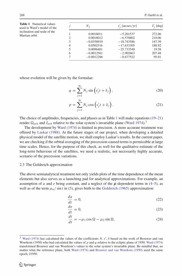
Table 1 Numerical valuesused in Ward’s model of theinclination and node of theMartian orbit
j Nj s′j
[arcsec/yr] δ′j
[deg]
1 0.0018011 −5.201537 272.062 0.0018012 −6.570802 210.063 −0.0358910 −18.743586 147.394 0.0502516 −17.633305 188.925 0.0096481 −25.733549 19.586 −0.0012561 −2.902663 207.487 −0.0012286 −0.677522 95.01
whose evolution will be given by the formulae:
q =∞∑
j=1
Nj sin(s′j t + δj
), (20)
p =∞∑
j=1
Nj cos(s′j t + δj
). (21)
The choice of amplitudes, frequencies, and phases as in Table 1 will make equations (19–21)render orb and Iorb relative to the solar system’s invariable plane (Ward 1974).3
The development by Ward (1974) is limited in precision. A more accurate treatment wasoffered by Laskar (1988). At the future stages of our project, when developing a detailedphysical model of the satellite motion, we shall employ Laskar’s results. In the current paper,we are checking if the orbital averaging of the precession-caused terms is permissible at largetime scales. Hence, for the purpose of this check, as well for the qualitative estimate of thelong-term behaviour of the satellites, we need a realistic, not necessarily highly accurate,scenario of the precession variations.
2.3 The Goldreich approximation
The above semianalytical treatment not only yields plots of the time dependence of the meanelements but also serves as a launching pad for analytical approximations. For example, anassumption of a and e being constant, and a neglect of the µ-dependent terms in (4–5), aswell as of the term µn/ sin i in (5), gives birth to the Goldreich (1965) approximation:
da
dt= 0, (22)
de
dt= 0, (23)
di
dt= −µ1 cos − µ2 sin , (24)
3 Ward (1974) has calculated the values of the coefficients N, s′, δ based on the work of Brouwer and vanWoerkom (1950) who had calculated the values of p and q relative to the ecliptic plane of 1950. Ward (1974)transformed Brouwer and van Woerkom’s values to the solar system’s invariable plane. Be mindful that, nomatter what the reference plane, both Ward (1974) and Brouwer and van Woerkom (1950) used the sameepoch, J1950.
123
Long-term evolution of orbits 269
d
dt= −3
2nJ2
(ρe
a
)2 cos i
(1 − e2)2 , (25)
dω
dt= 3
4n J2
(ρe
a
)2 5 cos2 i − 1
(1 − e2)2 + µn cos i
sin i− µ⊥, (26)
the equinoctial precession being assumed uniform:
Ip = 0 (27)
hp = −α cos Ip (28)
µ1 = 0 (29)
µ2 = hp sin Ip (30)
µ3 = hp cos Ip. (31)
For the details of Goldreich’s approximation see also Subsect. 3.3 in Efroimsky (2005).
2.4 The gravitational pull of the Sun
Reaction of a satellite on the planetary-equator precession is, in a way, an indirect reactionof the satellite on the presence of the Sun and the other planets. Indeed, the pull of the otherplanets makes the orbit of our planet precess, which entails variations in the Sun-producedgravitational torque acting on the planet. These variations of the torque, in their turn, lead tothe variable equinoctial precession of the equator, precession “felt” by the satellite. It wouldbe unphysical to consider this, indirect effect of the Sun and the planets upon the satellite,without taking into account their direct gravitational pull. In this subsection, we shall takeinto account the pull of the Sun, which greatly dominates that of the planets other than theprimary.
In what follows, m and m′ will be the masses of the satellite and the Sun, correspondingly,r and r′ will stand for the planetocentric positions of the satellite and the Sun, S will signifythe angle between these vectors. Then the Sun-caused perturbing potential RS , acting on thesatellite, will assume the form of
RS = Gm′(
1
|r′ − r| − r′ · rr ′3
)= Gm′
r ′
(r ′
|r′ − r| − r cos S
r ′
)(32)
This can be expanded in a usual manner over the Legendre polynomials of the first kind.Since r ′ r , we shall take only the first term in the series:4
RS ≈ Gm′
r ′
[1 + r
r ′ P1(cos S) +( r
r ′)2
P2(cos S) − r cos S
r ′
](33)
As the term Gm′/r ′ is not dependent of the satellite’s elements, one has only to considerthe restricted potential
R1S = Gm′
r ′
[( r
r ′)2
P2(cos S)
]≈ n′2a2
2
(a′
r ′
)3
(3 cos2 S − 1), (34)
n′ and a′ being the mean motion and the semi-major axis of the Sun.To obtain the Lagrange-type equations for the third-body perturbation, we must first
derive an expression for the angle S. To that end, define the directional cosines ξ ≡ P · r′ and
4 This is justified since the next term in the Legendre series is about 2 orders of magnitude smaller than thepotential variations generated by the precession.
123
270 P. Gurfil et al.
θ ≡ Q · r′, where r′ is a unit vector pointing from the planet toward the Sun, while P and Qare unit vectors of a perifocal coordinate system associated with the osculating orbital planeof the satellite, with P pointing to the instantaneous periapse and Q being orthogonal to P.Assuming that the planet’s orbit about the Sun is circular, we arrive at
ξ = cos ω cos( − M ′) − cos i sin ω sin( − M ′), (35)
θ = − sin ω cos( − M ′) − cos i cos ω sin( − M ′), (36)
where M ′ is the mean anomaly of the Sun in the planetocentric frame. With aid of theserelations, the angle S may be written down as
cos S = ξ cos ν + θ sin ν, (37)
ν being the true anomaly of the satellite in the planetocentric coordinate system. Substituting(35) and (36) into (37), and averaging over the satellite’s mean anomaly, we arrive at theLagrange-type equations:
da
dτ= 0 (38a)
de
dτ= 10 e
√1 − e2
[sin2 i sin 2ω + (2 − sin2 i) sin 2ω cos 2
+ 2 cos i cos 2ω sin 2]
(38b)
di
dτ= − 2 sin i√
1 − e2
5e2 cos i sin 2ω(1 − cos 2)
− [2 + e2(3 + 5 cos 2ω)
]sin 2
(38c)
dω
dτ= 2√
1 − e2
4 + e2 − 5 sin2 i + 5(sin2 i − e2) cos 2ω + 5(e2 − 2)
× cos i sin 2ω sin 2 + [5(2 − e2 − sin2 i) cos 2ω − 2 − 3 e2 + 5 sin2 i
]
× cos 2
(38d)
d
dτ= −κ − 2√
1 − e2
[2 + e2(3 − 5 cos 2ω)
](1 − cos 2) cos i
−5e2 sin 2ω sin 2
(38e)
where we used the following set of notations:
τ ≡ βn(t − t0), β = 3 m′a3
16 M a′3 (39)
κ ≡ 16 n
3 n′
(1 + M
m′
)(40)
123
Long-term evolution of orbits 271
≡ − λ′, (41)
λ′ being the mean longitude of the Sun in the planet’s frame, and M being the massof Mars.
An additional averaging can be performed over the motion of the planet about the Sun.Mathematically, this is the same as averaging over the motion of the Sun about the planet—inboth cases averaging over λ′ is implied. This averaging (Innanen et al. 1997) will simplify(38) into
da
dt= 0 (42a)
de
dt= 10e
√1 − e2βn sin2 i sin 2ω (42b)
di
dt= −10e2 sin i√
1 − e2βn cos i sin 2ω (42c)
dω
dt= 2√
1 − e2βn
[4 + e2 − 5 sin2 i + 5(sin2 i − e2) cos 2ω
](42d)
d
dt= − 2√
1 − e2βn
[2 + e2(3 − 5 cos 2ω)
]cos i (42e)
It is important to note that the calculations leading to equations (38), and to their double-averaged version, (42), were performed in the Martian-orbital, and not Martian-equatorialframe, without taking either the Martian obliquity or precession into consideration. Had wetaken into account the precession, we would get, on the right-hand side of (42) resonancesbetween the motion of the Sun relative to the planet and the equinoctial precession. Since thetime scale of the former exceeds, by orders of magnitude, the time scale of the latter, we maysafely omit such resonances. This justifies our neglect of the frame precession in the abovecalculation.
However, the omission of the obliquity may have a serious effect on the results. Thus, weshall generalize equations (38) so as to include the effect of the solar inclination and nodein a Martian-centric frame. This generalized model based on the celebrated works by Kozai(1959) and Cook (1962) gives us:
da
dt= 0 (43a)
de
dt= −15n′2e
√1 − e2
4n
[2AB cos(2ω) − (A2 − B2) sin(2ω)
](43b)
di
dt= 3n′2C
4n√
1 − e2
A
[2 + 3e2 + 5e2 cos(2ω)
] + 5Be2 sin(2ω)
(43c)
dω
dt= − cos i + 3n′2√1 − e2
2n
×[
5AB sin(2ω) + 5
2(A2 − B2) cos(2ω) − 1 + 3(A2 + B2)
2
]
+15n′2a(A cos ω + B sin ω)
4nea′
[1 − 5
4(A2 + B2)
](43d)
d
dt= 3n′2C
4n√
1 − e2 sin i
5Ae2 sin(2ω) + B
[2 + 3e2 − 5e2 cos(2ω)
](43e)
123
272 P. Gurfil et al.
where
A = cos( − ′) cos(λ′) + cos(i′) sin(λ′) sin( − ′) (44a)
B = cos i[− sin( − ′) cos(λ′) + cos(i′) sin(λ′) cos( − ′)
]
+ sin i sin(i′) sin(λ′) (44b)
C = sin i[cos λ′ sin( − ′) − cos(i′) sin(λ′) cos( − ′)
]
+ cos i sin i′ sin λ′ (44c)
Here, i′ and ′ are the inclination and right ascension of the ascending node of the Solarorbit in the Martian equatorial frame, respectively. The doubly averaged equations, obtainedafter averaging over the Sun’s mean anomaly for a single period, are given by
da
dt= 0 (45a)
de
dt= −15n′2e
√1 − e2
4n
[2AB cos(2ω) − (A2 − B2) sin(2ω)
](45b)
di
dt= 3n′2
4n√
1 − e2
CA
[2 + 3e2 + 5e2 cos(2ω)
] + 5CBe2 sin(2ω)
(45c)
dω
dt= − cos i + 3n′2√1 − e2
2n
×[
5AB sin(2ω) + 5
2(A2 − B2) cos(2ω) − 1 + 3(A2 + B2)
2
]
(45d)
d
dt= 3n′2
4n√
1 − e2 sin i
5CAe2 sin(2ω) + CB
[2 + 3e2 − 5e2 cos(2ω)
](45e)
the averaged quantities A2, B2, AB,AC,BC being given by
A2 = [s2i′c
2′ − 0.5 s2
i′]
c2 + s2
i′s′s′sc′c + 0.5 − 0.5s2i′c
2′ (46a)
B2 = (s2i′c
2′ + 0.5s2
i′)
c2 − s′s2
i′sc′c + 0.5s2i′c
2′ − 0.5 + c2
i′
c2i
+ (ci′cc′ + ci′ss′) si′sici + 0.5s2i′ (46b)
AB = s2i′s′c′c2
+ [−s2i′sc2
′ + 0.5s2i′s
]c − 0.5s2
i′s′c′
ci
+ 0.5ci′ (sc′ − cs′) si′si (46c)
AC = 0.5 ci′ (sc′ − cs′) si′ci
+ −s2i′s′c′c2
+ [−s2i′((s)2c2
′)]
c + 0.5s2i′s′c′
si (46d)
BC = (ci′cc′ + ci′ss′) si′c2i
+ [s2i′ (c′)2 − 0.5 (si′)
2] c2 − s2
i′s′sc′c + −0.5s2i′c
2′ − c2
i′ + 0.5
sici
− 0.5 (ci′ss′ + ci′cc′) si′ (46e)
where we have used the compact notation c(·) = cos(·), s(·) = sin(·). To calculate the trig-onometric functions of ′ and i′ appearing in equations (46), we shall utilise the geometryrendered Fig. 1. The figure depicts the Martian spin axis, k, that is perpendicular to the equa-tor of date, and the normal to the orbital plane (ecliptic of date), n. The Martian obliquity, ε,is the angle between these two vectors, and is calculated based on the Colombo formalism:
cos ε = k · n = q sx + p sy + F sz (47)
123
Long-term evolution of orbits 273
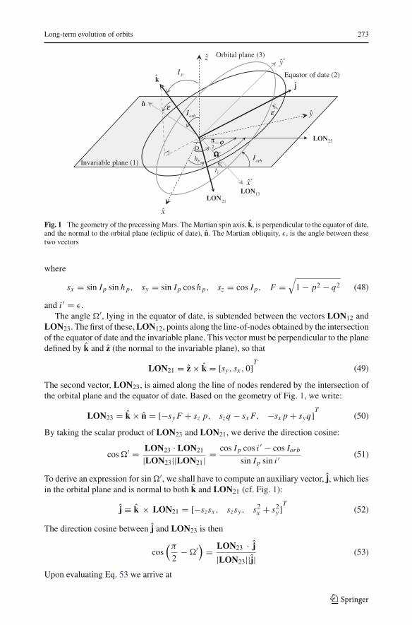
Fig. 1 The geometry of the precessing Mars. The Martian spin axis, k, is perpendicular to the equator of date,and the normal to the orbital plane (ecliptic of date), n. The Martian obliquity, ε, is the angle between thesetwo vectors
where
sx = sin Ip sin hp, sy = sin Ip cos hp, sz = cos Ip, F =√
1 − p2 − q2 (48)
and i′ = ε.The angle ′, lying in the equator of date, is subtended between the vectors LON12 and
LON23. The first of these, LON12, points along the line-of-nodes obtained by the intersectionof the equator of date and the invariable plane. This vector must be perpendicular to the planedefined by k and z (the normal to the invariable plane), so that
LON21 = z × k = [sy, sx, 0]T (49)
The second vector, LON23, is aimed along the line of nodes rendered by the intersection ofthe orbital plane and the equator of date. Based on the geometry of Fig. 1, we write:
LON23 = k × n = [−syF + sz p, szq − sxF, −sxp + syq]T (50)
By taking the scalar product of LON23 and LON21, we derive the direction cosine:
cos ′ = LON23 · LON21
|LON23||LON21| = cos Ip cos i′ − cos Iorb
sin Ip sin i′(51)
To derive an expression for sin ′, we shall have to compute an auxiliary vector, j, which liesin the orbital plane and is normal to both k and LON21 (cf. Fig. 1):
j ≡ k × LON21 = [−szsx, szsy, s2x + s2
y ]T (52)
The direction cosine between j and LON23 is then
cos(π
2− ′) = LON23 · j
|LON23||j|(53)
Upon evaluating Eq. 53 we arrive at
123
274 P. Gurfil et al.
sin ′ = q cos hp − p sin hp
sin i′(54)
Finally, the calculation of the orbital-elements’ evolution is performed via Lagrange-typeplanetary equations, whose right-hand sides combine those of (1)–(5) and (45).
2.5 The higher-order harmonics, the gravitational pull of the planets,the Yarkovsky effect, and the bodily tides
In the current paper, we pursue a limited goal of taking into account the oblateness of theplanet, its nonuniform equinoctial precession, and the gravitational pull of the Sun. Thesethree items certainly do not exhaust the list of factors influencing the orbit evolution of asatellite.
Among the factors that we intend to include into the model at the further stage of its devel-opment are the high-order zonal (J3, J4, J
22 ) and tesseral (C22) harmonics of the planet’s
gravity field, as well as the gravitational pull of the other planets—factors whose role wascomprehensively discussed, for example, by Waz (2004). We also intend to include the bodilytides (Efroimsky and Lainey 2007) and the Yarkovsky effect (Nesvorný and Vokrouhlický2007)—factors whose importance increases at long time scales.
3 Comparison of a purely numerical and a semianalytical treatmentof the problem
One of our goals is to check the applicability limits (both in terms of the initial conditions andthe permissible time scales) of our semianalytical model written for the osculating elementsintroduced in a frame co-precessing with the equator of date. This check will be performed byan independent, purely numerical, computation that will be free from whatever simplifyingassumptions (all terms kept, no averaging performed.) The straightforward simulation will becarried out in terms of Cartesian coordinates and velocities defined in an inertial frame of ref-erence. Both the semianalytical calculation of the elements in a co-precessing frame and thestraightforward numerical integration in inertial Cartesian axes will be carried out for Deimos.
3.1 Integration by a purely numerical approach
The numerical integration of Deimos’ orbit can be performed using Cartesian coordinatesdefined relatively to the Solar system invariable plane. As we also have to compute theMartian polar axis motion, there are two vector differential equations to integrate simulta-neously. One is the Newton gravity law:
r = −G(M + m)rr3 + Gm′
(r′ − r
|r′ − r|3 − r′
r ′3
)+ G(M + m)∇U, (55)
where ∇U has components⎧⎪⎪⎪⎪⎪⎪⎪⎨
⎪⎪⎪⎪⎪⎪⎪⎩
∂xU = ρ2e J2
r4
[x
r
(15
2sin2 φ − 3
2
)− 3 sin φ sin Ip sin hp
]
∂yU = ρ2e J2
r4
[y
r
(15
2sin2 φ − 3
2
)+ 3 sin φ sin Ip cos hp
]
∂zU = ρ2e J2
r4
[z
r
(15
2sin2 φ − 3
2
)− 3 sin φ cos Ip
].
(56)
123
Long-term evolution of orbits 275
Here φ and r = (x, y, z) denote, correspondingly, the latitude of Deimos relative to theMartian equator and the position vector of Deimos related to the Martian center of mass; ρe
is the Martian equatorial radius; M and m stand for the masses of Mars and Deimos, respec-tively. Angles hp and Ip are the longitude of the node and the inclination of the planet’sequator of date relative to the invariable plane (see Sect. 2.2). Integration in this, inertial,frame offers the obvious advantage of nullifying the inertial forces.
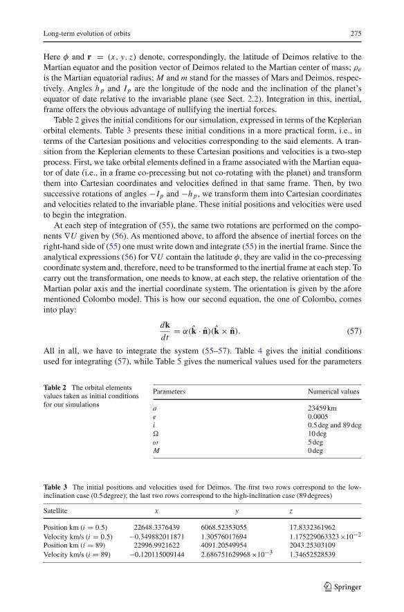
Table 2 gives the initial conditions for our simulation, expressed in terms of the Keplerianorbital elements. Table 3 presents these initial conditions in a more practical form, i.e., interms of the Cartesian positions and velocities corresponding to the said elements. A tran-sition from the Keplerian elements to these Cartesian positions and velocities is a two-stepprocess. First, we take orbital elements defined in a frame associated with the Martian equa-tor of date (i.e., in a frame co-precessing but not co-rotating with the planet) and transformthem into Cartesian coordinates and velocities defined in that same frame. Then, by twosuccessive rotations of angles −Ip and −hp , we transform them into Cartesian coordinatesand velocities related to the invariable plane. These initial positions and velocities were usedto begin the integration.
At each step of integration of (55), the same two rotations are performed on the compo-nents ∇U given by (56). As mentioned above, to afford the absence of inertial forces on theright-hand side of (55) one must write down and integrate (55) in the inertial frame. Since theanalytical expressions (56) for ∇U contain the latitude φ, they are valid in the co-precessingcoordinate system and, therefore, need to be transformed to the inertial frame at each step. Tocarry out the transformation, one needs to know, at each step, the relative orientation of theMartian polar axis and the inertial coordinate system. The orientation is given by the aforementioned Colombo model. This is how our second equation, the one of Colombo, comesinto play:
dkdt
= α(k · n)(k × n). (57)
All in all, we have to integrate the system (55–57). Table 4 gives the initial conditionsused for integrating (57), while Table 5 gives the numerical values used for the parameters
Table 2 The orbital elementsvalues taken as initial conditionsfor our simulations
Parameters Numerical values
a 23459 kme 0.0005i 0.5 deg and 89 deg 10 degω 5 degM 0 deg
Table 3 The initial positions and velocities used for Deimos. The first two rows correspond to the low-inclination case (0.5 degree); the last two rows correspond to the high-inclination case (89 degrees)
Satellite x y z
Position km (i = 0.5) 22648.3376439 6068.52353055 17.8332361962Velocity km/s (i = 0.5) −0.349882011871 1.30576017694 1.175229063323×10⁻²
Position km (i = 89) 22996.9921622 4091.20549954 2043.25303109Velocity km/s (i = 89) −0.120115009144 2.686751629968×10⁻³ 1.34652528539
123
276 P. Gurfil et al.
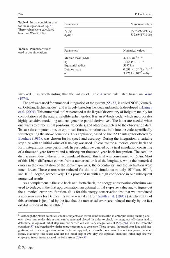
Table 4 Initial conditions usedfor the integration of Eq. 57.These values were calculatedbased on Ward (1974)
Parameters Numerical values
Ip(t0) 25.25797549 deghp(t0) 332.6841708 deg
Table 5 Parameter valuesused in our simulations
Parameters Numerical values
Martian mass (GM) 42830 km3 s−2
J2 1960.45 × 10−6
Equatorial radius 3397 kmDeimos mass 0.091 × 10⁻³ km3 s−2
α 3.9735 × 10⁻⁵ rad/yr
involved. It is worth noting that the values of Table 4 were calculated based on Ward(1974).
The software used for numerical integration of the system (55–57) is called NOE (Numeri-cal Orbit and Ephemerides), and is largely based on the ideas and methods developed in Laineyet al. (2004). This numerical tool was created at the Royal Observatory of Belgium mainly forcomputations of the natural satellite ephemerides. It is an N -body code, which incorporateshighly sensitive modelling and can generate partial derivatives. The latter are needed whenone wants to fit the initial positions, velocities, and other parameters to the observation data.To save the computer time, an optimised force subroutine was built into the code, specificallyfor integrating the above equations. This appliance, based on the RA15 integrator offered byEverhart (1985), was chosen for its speed and accuracy. During the integration, a variablestep size with an initial value of 0.04 day was used. To control the numerical error, back andforth integrations were performed. In particular, we carried out a trial simulation consistingof a thousand-year forward and a subsequent thousand-year back integration. The satellitedisplacement due to the error accumulated through this trial was constrained to 150 m. Mostof this 150 m difference comes from a numerical drift of the longitude, while the numericalerrors in the computation of the semi-major axis, the eccentricity, and the inclination weremuch lower. These errors were reduced for this trial simulation to only 10−5 km, 10−10,and 10−10 degree, respectively. This provided us with a high confidence in our subsequentnumerical results.
As a complement to the said back-and-forth check, the energy-conservation criterium wasused to deduce, in the first approximation, an optimal initial step-size value and to figure outthe numerical error proliferation. (It is for this energy-conservation test that we introduceda non-zero mass for Deimos. Its value was taken from Smith et al. (1995).) Applicability ofthis criterium is justified by the fact that the numerical errors are induced mostly by the fastorbital motion of the satellite.5
5 Although the planet-satellite system is subject to an external influence (the solar torque acting on the planet),over short time scales this system can be assumed closed. In order to check the integrator efficiency and todetermine an optimal initial step size, we carried out auxiliary integrations of (55)–(56), with the Colomboequation (57) neglected and with the energy presumed to conserve. These several-thousand-year-long trial inte-grations, with the energy-conservation criterium applied, led us to the conclusion that our integrator remainedsteady over long time scales and that the initial step of 0.04 day was optimal. Then this initial step size wasemployed in our integration of the full system (55)–(57).
123
Long-term evolution of orbits 277
3.2 Integration by the semianalytical approach
The theory of satellite-orbit evolution, based on the planetary equations whose right-handsides combine those of (1–5) and (45), is semianalytical. This means that these equations forthe elements’ secular parts are derived analytically, but their integration is to be performednumerically. This integration was carried out using an 8th-order Runge-Kutta scheme withrelative and absolute tolerances of 10−12. Kilograms, years, and kilometers were taken asthe mass, time, and length units, correspondingly.
3.2.1 Technicalities
To integrate the planetary equations, one should know, at each time step, the values of Ip andhp, which are the time derivatives of the inclination and of the longitude of the node of theequator of date with respect to the equator of epoch. These derivatives will be rendered bythe Colombo equation (17), after formulae (15–16) get inserted therein:
Ip = −α
(q2 sin Ip sin hp cos hp − qp sin Ip + 2pq sin Ip cos2 hp
−p2 sin Ip cos hp sin hp + q
√1 − q2 − p2 cos Ip cos hp
− p
√1 − q2 − p2 cos Ip sin hp
), (58)
and
hp = −α
[(p − 2p cos2 Ip
)cos hp +
(−q + 2q cos2 Ip
)cos2 hp − 2q cos2 Ip + q
sin hp
]
×√
1 − p2 − q2
sin Ip
+ (q2 − p2) cos Ip cos2 hp + (−p2 − 2q2 + 1
)cos Ip
+ 2qp cos Ip cos3 hp − 2pq cos hp cos Ip
sin hp
. (59)
Equations (58) and (59) are then integrated (with the initial conditions Ip(t0) and hp(t0) bor-rowed from Table 4) simultaneously with the planetary equations (1–5). Through formulae(6), the above expressions for Ip and hp yield the expressions for the components of µ. Ascan be seen from (12–14), integration of the planetary equations also requires the knowledgeof the derivatives µ1 , µ2, and µ3 at each integration step. These can be readily obtainedby differentiating (6). The resulting closed-formed expressions for µ1, µ2, µ3 are listed inAppendix A. The final step required for numerical integration of the planetary equations issubstitution of formulae (9–11), with the initial conditions from Table 2.
3.2.2 The plots and their interpretation
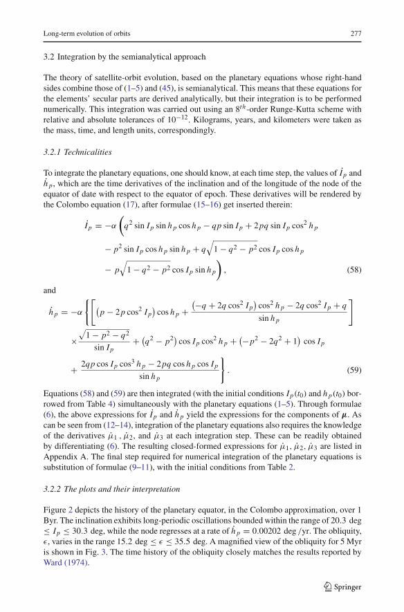
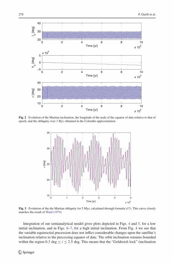
Figure 2 depicts the history of the planetary equator, in the Colombo approximation, over 1Byr. The inclination exhibits long-periodic oscillations bounded within the range of 20.3 deg≤ Ip ≤ 30.3 deg, while the node regresses at a rate of hp = 0.00202 deg /yr. The obliquity,ε, varies in the range 15.2 deg ≤ ε ≤ 35.5 deg. A magnified view of the obliquity for 5 Myris shown in Fig. 3. The time history of the obliquity closely matches the results reported byWard (1974).
123
278 P. Gurfil et al.
0 2 4 6 8 10
x 108
20
30
40
Time [yr]
I p [deg
]
0 2 4 6 8 10
x 108
−5
0
5x 10
6
Time [yr]
h p [deg
]
0 2 4 6 8 10
x 108
10
20
30
40
Time [yr]
ε [d
eg]
Fig. 2 Evolution of the Martian inclination, the longitude of the node of the equator of date relative to that ofepoch, and the obliquity over 1 Byr, obtained in the Colombo approximation
0 1 2 3 4 5
x 106
15
20
25
30
35
Time [yr]
ε [d
eg]
Fig. 3 Evolution of the the Martian obliquity for 5 Myr, calculated through formula (47). This curve closelymatches the result of Ward (1974)
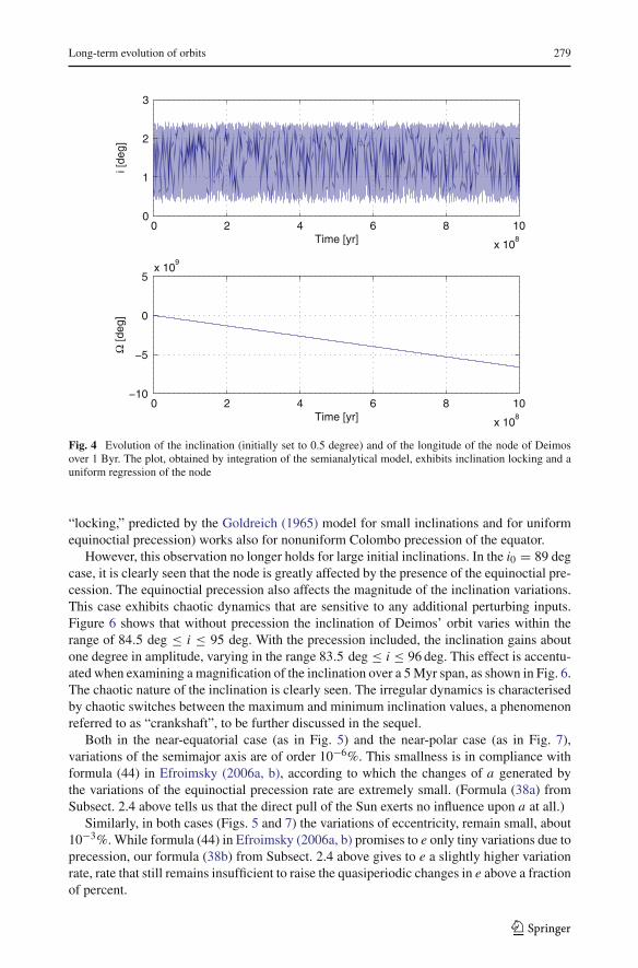
Integration of our semianalytical model gives plots depicted in Figs. 4 and 5, for a lowinitial inclination, and in Figs. 6–7, for a high initial inclination. From Fig. 4 we see thatthe variable equinoctial precession does not inflict considerable changes upon the satellite’sinclination relative to the precessing equator of date. The orbit inclination remains boundedwithin the region 0.3 deg ≤ i ≤ 2.5 deg. This means that the “Goldreich lock” (inclination
123
Long-term evolution of orbits 279
0 2 4 6 8 10
x 108
0
1
2
3
Time [yr]
i [de
g]
0 2 4 6 8 10
x 108
−10
−5
0
5x 10
9
Time [yr]
Ω [d
eg]
Fig. 4 Evolution of the inclination (initially set to 0.5 degree) and of the longitude of the node of Deimosover 1 Byr. The plot, obtained by integration of the semianalytical model, exhibits inclination locking and auniform regression of the node
“locking,” predicted by the Goldreich (1965) model for small inclinations and for uniformequinoctial precession) works also for nonuniform Colombo precession of the equator.
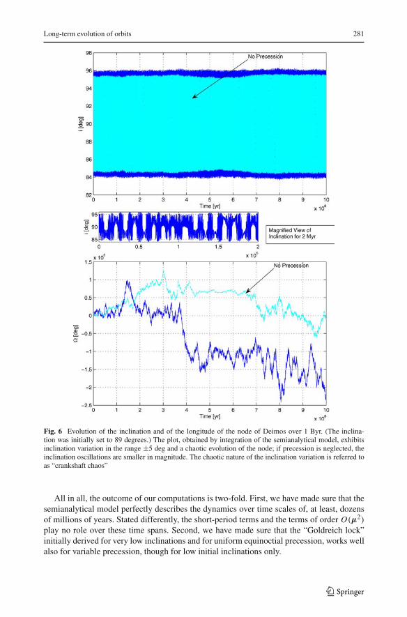
However, this observation no longer holds for large initial inclinations. In the i0 = 89 degcase, it is clearly seen that the node is greatly affected by the presence of the equinoctial pre-cession. The equinoctial precession also affects the magnitude of the inclination variations.This case exhibits chaotic dynamics that are sensitive to any additional perturbing inputs.Figure 6 shows that without precession the inclination of Deimos’ orbit varies within therange of 84.5 deg ≤ i ≤ 95 deg. With the precession included, the inclination gains aboutone degree in amplitude, varying in the range 83.5 deg ≤ i ≤ 96 deg. This effect is accentu-ated when examining a magnification of the inclination over a 5 Myr span, as shown in Fig. 6.The chaotic nature of the inclination is clearly seen. The irregular dynamics is characterisedby chaotic switches between the maximum and minimum inclination values, a phenomenonreferred to as “crankshaft”, to be further discussed in the sequel.
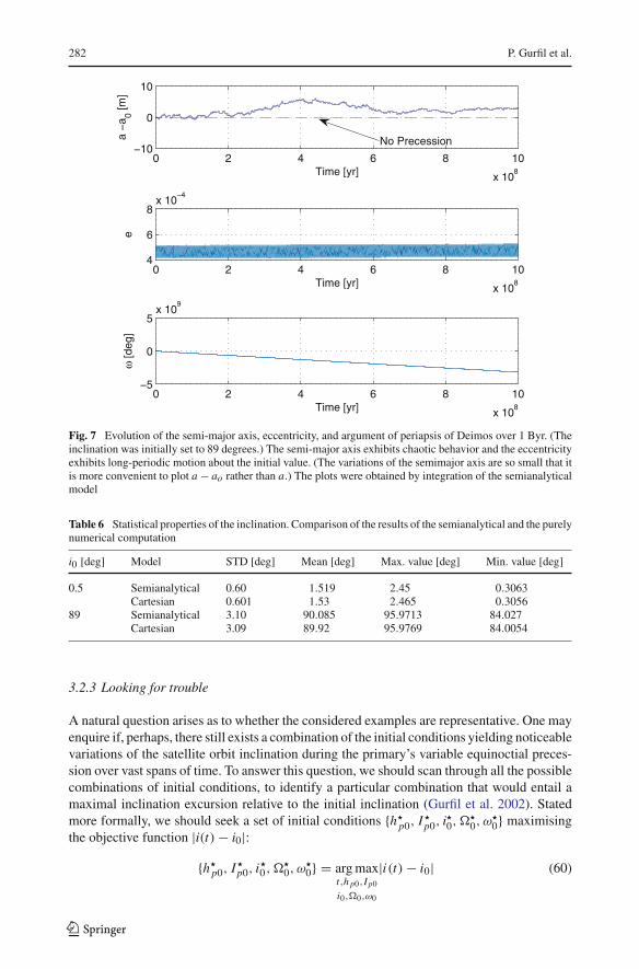
Both in the near-equatorial case (as in Fig. 5) and the near-polar case (as in Fig. 7),variations of the semimajor axis are of order 10−6%. This smallness is in compliance withformula (44) in Efroimsky (2006a, b), according to which the changes of a generated bythe variations of the equinoctial precession rate are extremely small. (Formula (38a) fromSubsect. 2.4 above tells us that the direct pull of the Sun exerts no influence upon a at all.)
Similarly, in both cases (Figs. 5 and 7) the variations of eccentricity, remain small, about10−3%. While formula (44) in Efroimsky (2006a, b) promises to e only tiny variations due toprecession, our formula (38b) from Subsect. 2.4 above gives to e a slightly higher variationrate, rate that still remains insufficient to raise the quasiperiodic changes in e above a fractionof percent.
123
280 P. Gurfil et al.
Fig. 5 Evolution of the semimajor axis, eccentricity, and argument of periapsis of Deimos over 1 Byr. (Theinclination was initially set to 0.5 degree.) Both the semimajor axis and eccentricity exhibit quasiperiodicmotion about their initial values. (The variations of the semimajor axis and eccentricity are so small that itis more convenient to plot a − a0 and e − e0.) The plots were obtained by integration of the semianalyticalmodel
The plots in Figs. 5 and 7 depict also the time evolution of ω. The line of apsides steadilyregresses in the near-polar case and steadily advances in the near-equatorial case.
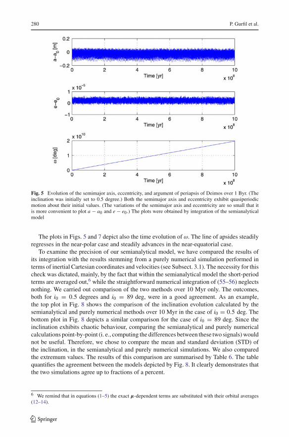
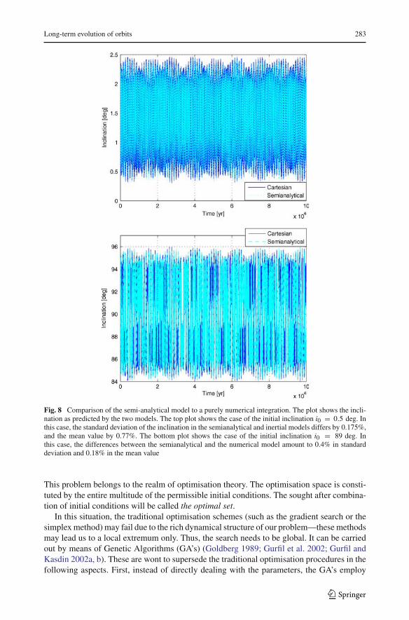
To examine the precision of our semianalytical model, we have compared the results ofits integration with the results stemming from a purely numerical simulation performed interms of inertial Cartesian coordinates and velocities (see Subsect. 3.1). The necessity for thischeck was dictated, mainly, by the fact that within the semianalytical model the short-periodterms are averaged out,6 while the straightforward numerical integration of (55–56) neglectsnothing. We carried out comparison of the two methods over 10 Myr only. The outcomes,both for i0 = 0.5 degrees and i0 = 89 deg, were in a good agreement. As an example,the top plot in Fig. 8 shows the comparison of the inclination evolution calculated by thesemianalytical and purely numerical methods over 10 Myr in the case of i0 = 0.5 deg. Thebottom plot in Fig. 8 depicts a similar comparison for the case of i0 = 89 deg. Since theinclination exhibits chaotic behaviour, comparing the semianalytical and purely numericalcalculations point-by-point (i. e., computing the differences between these two signals) wouldnot be useful. Therefore, we chose to compare the mean and standard deviation (STD) ofthe inclination, in the semianalytical and purely numerical simulations. We also comparedthe extremum values. The results of this comparison are summarised by Table 6. The tablequantifies the agreement between the models depicted by Fig. 8. It clearly demonstrates thatthe two simulations agree up to fractions of a percent.
6 We remind that in equations (1–5) the exact µ-dependent terms are substituted with their orbital averages(12–14).
123
Long-term evolution of orbits 281
Fig. 6 Evolution of the inclination and of the longitude of the node of Deimos over 1 Byr. (The inclina-tion was initially set to 89 degrees.) The plot, obtained by integration of the semianalytical model, exhibitsinclination variation in the range ±5 deg and a chaotic evolution of the node; if precession is neglected, theinclination oscillations are smaller in magnitude. The chaotic nature of the inclination variation is referred toas “crankshaft chaos”
All in all, the outcome of our computations is two-fold. First, we have made sure that thesemianalytical model perfectly describes the dynamics over time scales of, at least, dozensof millions of years. Stated differently, the short-period terms and the terms of order O(µ2)
play no role over these time spans. Second, we have made sure that the “Goldreich lock”initially derived for very low inclinations and for uniform equinoctial precession, works wellalso for variable precession, though for low initial inclinations only.
123
282 P. Gurfil et al.
0 2 4 6 8 10
x 108
−10
0
10
Time [yr]
a −
a 0 [m]
0 2 4 6 8 10
x 108
4
6
8x 10
−4
Time [yr]
e
0 2 4 6 8 10
x 108
−5
0
5x 10
9
Time [yr]
ω [d
eg]
No Precession
Fig. 7 Evolution of the semi-major axis, eccentricity, and argument of periapsis of Deimos over 1 Byr. (Theinclination was initially set to 89 degrees.) The semi-major axis exhibits chaotic behavior and the eccentricityexhibits long-periodic motion about the initial value. (The variations of the semimajor axis are so small that itis more convenient to plot a − ao rather than a.) The plots were obtained by integration of the semianalyticalmodel
Table 6 Statistical properties of the inclination. Comparison of the results of the semianalytical and the purelynumerical computation
i0 [deg] Model STD [deg] Mean [deg] Max. value [deg] Min. value [deg]
0.5 Semianalytical 0.60 1.519 2.45 0.3063Cartesian 0.601 1.53 2.465 0.3056
89 Semianalytical 3.10 90.085 95.9713 84.027Cartesian 3.09 89.92 95.9769 84.0054
3.2.3 Looking for trouble
A natural question arises as to whether the considered examples are representative. One mayenquire if, perhaps, there still exists a combination of the initial conditions yielding noticeablevariations of the satellite orbit inclination during the primary’s variable equinoctial preces-sion over vast spans of time. To answer this question, we should scan through all the possiblecombinations of initial conditions, to identify a particular combination that would entail amaximal inclination excursion relative to the initial inclination (Gurfil et al. 2002). Statedmore formally, we should seek a set of initial conditions h
p0, Ip0, i0,
0, ω
0 maximising
the objective function |i(t) − i0|:h
p0, Ip0, i
0,
0, ω0 = arg max
t,hp0,Ip0
i0,0,ω0
|i(t) − i0| (60)
123
Long-term evolution of orbits 283
Fig. 8 Comparison of the semi-analytical model to a purely numerical integration. The plot shows the incli-nation as predicted by the two models. The top plot shows the case of the initial inclination i0 = 0.5 deg. Inthis case, the standard deviation of the inclination in the semianalytical and inertial models differs by 0.175%,and the mean value by 0.77%. The bottom plot shows the case of the initial inclination i0 = 89 deg. Inthis case, the differences between the semianalytical and the numerical model amount to 0.4% in standarddeviation and 0.18% in the mean value
This problem belongs to the realm of optimisation theory. The optimisation space is consti-tuted by the entire multitude of the permissible initial conditions. The sought after combina-tion of initial conditions will be called the optimal set.
In this situation, the traditional optimisation schemes (such as the gradient search or thesimplex method) may fail due to the rich dynamical structure of our problem—these methodsmay lead us to a local extremum only. Thus, the search needs to be global. It can be carriedout by means of Genetic Algorithms (GA’s) (Goldberg 1989; Gurfil et al. 2002; Gurfil andKasdin 2002a, b). These are wont to supersede the traditional optimisation procedures in thefollowing aspects. First, instead of directly dealing with the parameters, the GA’s employ
123
284 P. Gurfil et al.
Table 7 Parameter values usedfor the GA optimization
Parameters Numerical values
Population size 30Number of generations 100String length 16 bitProbability of crossover 0.99Probability of mutation 0.02
codings (usually, binary) of the parameter set (“strings,” in the GA terminology). Second,instead of addressing a single point of the optimisation space, the GAs perform a search insidea population of the initial conditions. Third, instead of processing derivatives or whateverother auxiliary information, the GAs use only objective-function evaluations (“fitness eval-uations”). Fourth, instead of deterministic rules to reiterate, the GAs rely upon probabilistictransition rules. Additional details on the particular GA mechanism used herein can be foundin Appendix B.
A GA optimisation was implemented using the parameter values given in Table 7.The search for the inclination-maximising initial conditions resulted in the following set:
I p0 = 72.5 deg, h
p0 = 211.324 deg, i0 = 100.543 deg,
0 = 111.538 deg, ω
0 = 234.913 deg . (61)
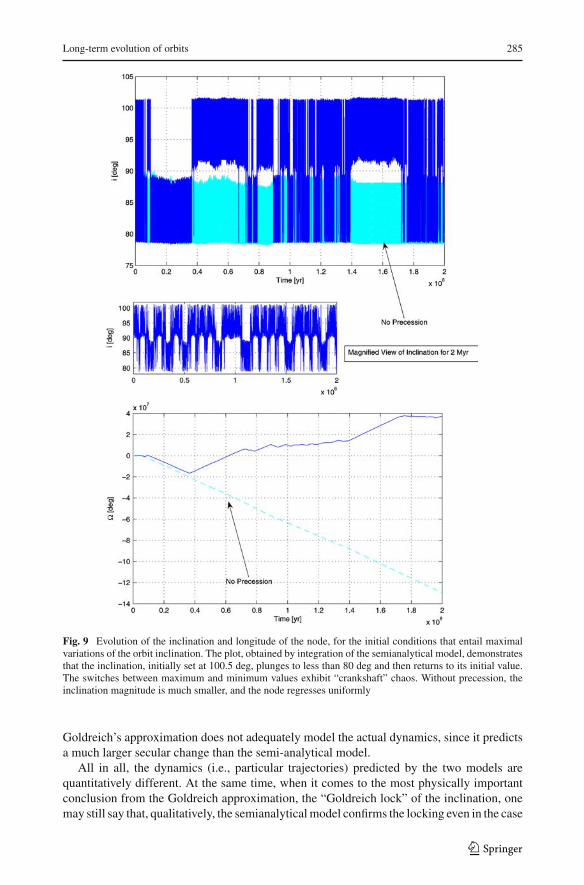
Thus, the initial orbit is retrograde and, not surprisingly, near-polar. The resulting time his-tories for a 0.2 Byr integration are depicted in Fig. 9, for i and . In both cases the inclinationamplitude is relatively large: The inclination varies within the range of 79 deg < i < 102 deg.
This example clearly shows that the equinoctial precession is an important effect forevolution of satellite orbits. As shown in the upper pane of Fig. 9, had we neglected theprecession, the magnitude of the oscillations would be about twice smaller. The inclusionof the precession in the model qualitatively modifies the behavior, inducing large-magnitudechaotic variations of the inclination, a phenomenon that cannot be detected without includingthe precession alongside the oblateness and solar gravity.
4 Comparison of the semianalytical results with those renderedby Goldreich’s model
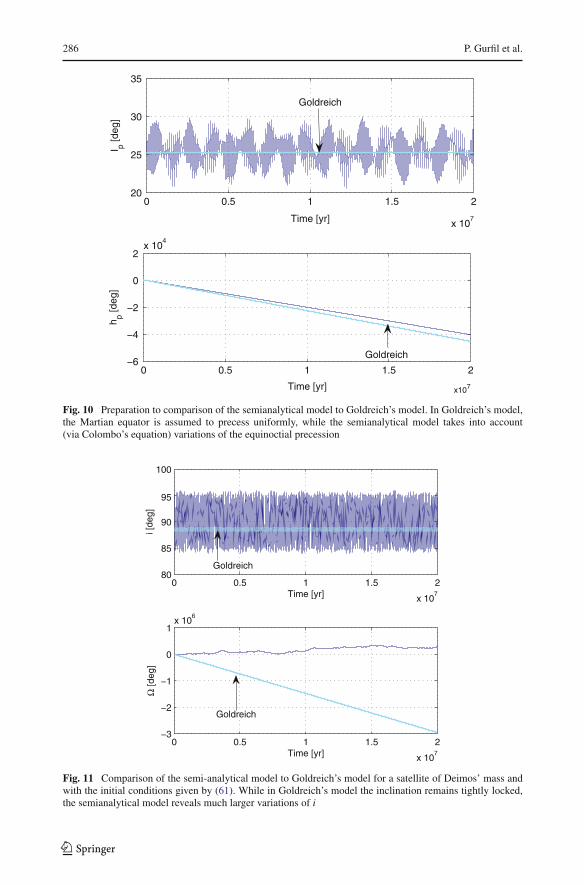
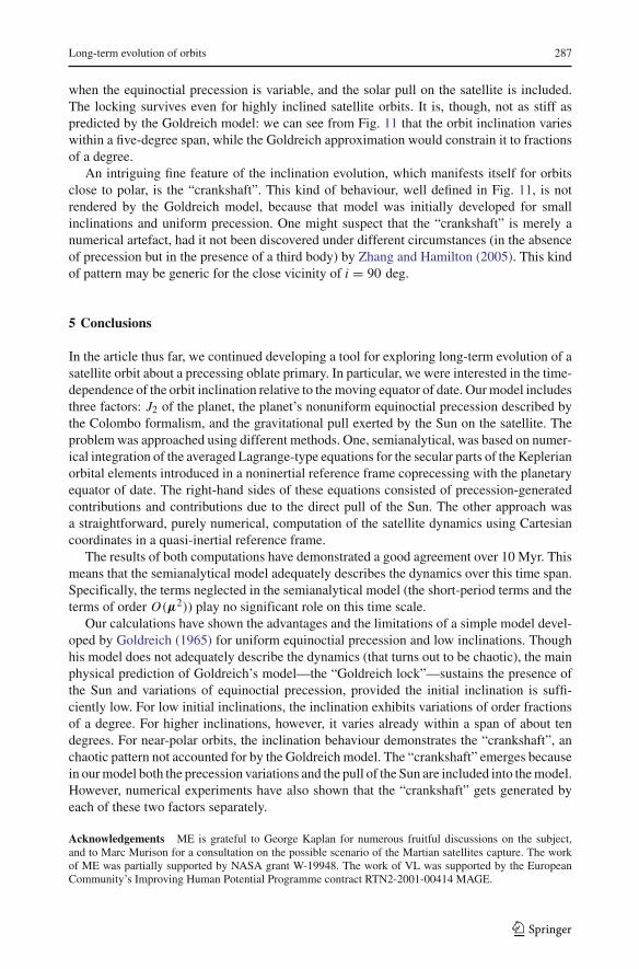
The final step in our study will be to compare the semianalytical model to Goldreich’s approx-imation (22–26). To that end, we integrate our semianalytical model for 20 Myr, using theinitial conditions from Table 2 with i0 = 89 deg; and compare the outcome with that resultingfrom Goldreich’s approximation simulated with the same initial conditions. The results of thiscomparison are depicted in Figs. 10 and 11. Specifically, Fig. 10 compares the time histories ofIp and hp . There are noticeable differences in the dynamics of Ip . While Goldreich’s approx-imation assumes a constant Ip , the semianalytical model is based on the Colombo calculationof the equinoctial precession, calculation that predicts considerable oscillations within therange 21 deg ≤ Ip ≤ 30 deg. Beside this, in our semianalytical model we take into accountthe direct gravitational pull exerted by the Sun on the satellite. All this entails differencesbetween the dynamics predicted by our semianalytical model and the dynamics stemmingfrom the Goldreich approximation. These differences, for i and , are depicted in Fig. 11.In Goldreich’s model, i stays very close to the initial value: 88.27 deg ≤ i ≤ 89.01 deg,a behaviour that makes the essence of the Goldreich lock. However, in the more accurate,semianalytical model we have 84 deg ≤ i ≤ 96 deg. The time history of , too, reveals that
123
Long-term evolution of orbits 285
Fig. 9 Evolution of the inclination and longitude of the node, for the initial conditions that entail maximalvariations of the orbit inclination. The plot, obtained by integration of the semianalytical model, demonstratesthat the inclination, initially set at 100.5 deg, plunges to less than 80 deg and then returns to its initial value.The switches between maximum and minimum values exhibit “crankshaft” chaos. Without precession, theinclination magnitude is much smaller, and the node regresses uniformly
Goldreich’s approximation does not adequately model the actual dynamics, since it predictsa much larger secular change than the semi-analytical model.
All in all, the dynamics (i.e., particular trajectories) predicted by the two models arequantitatively different. At the same time, when it comes to the most physically importantconclusion from the Goldreich approximation, the “Goldreich lock” of the inclination, onemay still say that, qualitatively, the semianalytical model confirms the locking even in the case
123
286 P. Gurfil et al.
0 0.5 1 1.5 2
x 107
20
25
30
35
Time [yr]
I p [deg
]
0 0.5 1 1.5 2
x107
−6
−4
−2
0
2x 10
4
Time [yr]
h p [deg
]Goldreich
Goldreich
Fig. 10 Preparation to comparison of the semianalytical model to Goldreich’s model. In Goldreich’s model,the Martian equator is assumed to precess uniformly, while the semianalytical model takes into account(via Colombo’s equation) variations of the equinoctial precession
0 0.5 1 1.5 2
x 107
80
85
90
95
100
Time [yr]
i [de
g]
0 0.5 1 1.5 2
x 107
−3
−2
−1
0
1x 10
6
Time [yr]
Ω [d
eg]
Goldreich
Goldreich
Fig. 11 Comparison of the semi-analytical model to Goldreich’s model for a satellite of Deimos’ mass andwith the initial conditions given by (61). While in Goldreich’s model the inclination remains tightly locked,the semianalytical model reveals much larger variations of i
123
Long-term evolution of orbits 287
when the equinoctial precession is variable, and the solar pull on the satellite is included.The locking survives even for highly inclined satellite orbits. It is, though, not as stiff aspredicted by the Goldreich model: we can see from Fig. 11 that the orbit inclination varieswithin a five-degree span, while the Goldreich approximation would constrain it to fractionsof a degree.
An intriguing fine feature of the inclination evolution, which manifests itself for orbitsclose to polar, is the “crankshaft”. This kind of behaviour, well defined in Fig. 11, is notrendered by the Goldreich model, because that model was initially developed for smallinclinations and uniform precession. One might suspect that the “crankshaft” is merely anumerical artefact, had it not been discovered under different circumstances (in the absenceof precession but in the presence of a third body) by Zhang and Hamilton (2005). This kindof pattern may be generic for the close vicinity of i = 90 deg.
5 Conclusions
In the article thus far, we continued developing a tool for exploring long-term evolution of asatellite orbit about a precessing oblate primary. In particular, we were interested in the time-dependence of the orbit inclination relative to the moving equator of date. Our model includesthree factors: J2 of the planet, the planet’s nonuniform equinoctial precession described bythe Colombo formalism, and the gravitational pull exerted by the Sun on the satellite. Theproblem was approached using different methods. One, semianalytical, was based on numer-ical integration of the averaged Lagrange-type equations for the secular parts of the Keplerianorbital elements introduced in a noninertial reference frame coprecessing with the planetaryequator of date. The right-hand sides of these equations consisted of precession-generatedcontributions and contributions due to the direct pull of the Sun. The other approach wasa straightforward, purely numerical, computation of the satellite dynamics using Cartesiancoordinates in a quasi-inertial reference frame.
The results of both computations have demonstrated a good agreement over 10 Myr. Thismeans that the semianalytical model adequately describes the dynamics over this time span.Specifically, the terms neglected in the semianalytical model (the short-period terms and theterms of order O(µ2)) play no significant role on this time scale.
Our calculations have shown the advantages and the limitations of a simple model devel-oped by Goldreich (1965) for uniform equinoctial precession and low inclinations. Thoughhis model does not adequately describe the dynamics (that turns out to be chaotic), the mainphysical prediction of Goldreich’s model—the “Goldreich lock”—sustains the presence ofthe Sun and variations of equinoctial precession, provided the initial inclination is suffi-ciently low. For low initial inclinations, the inclination exhibits variations of order fractionsof a degree. For higher inclinations, however, it varies already within a span of about tendegrees. For near-polar orbits, the inclination behaviour demonstrates the “crankshaft”, anchaotic pattern not accounted for by the Goldreich model. The “crankshaft” emerges becausein our model both the precession variations and the pull of the Sun are included into the model.However, numerical experiments have also shown that the “crankshaft” gets generated byeach of these two factors separately.
Acknowledgements ME is grateful to George Kaplan for numerous fruitful discussions on the subject,and to Marc Murison for a consultation on the possible scenario of the Martian satellites capture. The workof ME was partially supported by NASA grant W-19948. The work of VL was supported by the EuropeanCommunity’s Improving Human Potential Programme contract RTN2-2001-00414 MAGE.
123
288 P. Gurfil et al.
Appendix A: Closed-form expressions for µ1, µ2, µ3
Using the compact notation c(·) ≡ cos(·) and s(·) ≡ sin(·), and conforming to the proceduredescribed in the text, we obtain the following expressions for µ1, µ2, µ3:
µ1 = (((6 p2q2 − p4 − q4)(cIp )3 + (−6 p2q2 + p4 + q4)cIp )(chp )4
+ ((−3 p4 − 6 p2q2 − 3 q2 + 3 p2 + 5 q4)(cIp )3
+ (2 p4 − 4 q4 + 6 p2q2 − 2 p2 + 2 q2)cIp ) · (c(hp))2
+ (3 q2 − 3 p2q2 − 4 q4)(cIp )3 + (3 q4 − 2 q2 + 2 p2q2)cIp
+ (((4 qp3 − 4 q3p)(cIp )3 + (4 q3p − 4 qp3)cIp )(chp )5
+ ((2 qp3 − 6 qp + 14 q3p)(cIp )3
+ (−12 q3p + 4 qp)cIp )(chp )3 + ((6 qp − 10 q3p − 6 qp3)(cIp )3
+ (4 qp3 + 8 q3p − 4 qp)cIp )chp ) · (shp )−1)(sIp )−1
+ ((−9 pq2 + 9 pq4 − 3 p5 + 3 p3 + 6 p3q2)(cIp )2 + 3 pq2 − 2 p3q2 + p5
− 3pq4 − p3)(c3hp
+ ((−11 p3q2 − p5 − 10 pq4 − p + 2 p3 + 11 pq2)(c(Ip))2
+ 3pq4 + 3 p3q2 − 3pq2)chp + (((−9 p2q + 6 p2q3 + 9 p4q − 3 q5 + 3 q3)(cIp )2
− 3p4q + 3 p2q − 2 p2q3
− q3 + q5)(c4hp
+ ((7 p2q − p2q3 − 8 q3 − 8 p4q + 7 q5 + q)(cIp )2
− 2q5 + p2q3 + 2 q3
+ 3p4q − 3 p2q)(c(hp))2 + (5 q3 − 4 q5 − q − 5 p2q3 − p4q + 2 p2q)(cIp )2
− q3 + q5 + p2q3) ·(
s(hp))−1)
[√1 − p2 − q2
]−1)
α2
−α
(
(((−2 qp − 2 q p)(cIp )2 + 2 qp + 2 q p)(chp )2
+ (q p + qp)(cIp )2 − q p − qp + (((−2 pp + 2 qq)(cIp )2 + 2 pp − 2 qq)(chp )3
+ ((2 pp − 2 qq)(cIp )2 − 2 pp + 2 qq)chp )(s(hp))−1)(s(Ip))−1
+(
(−q p2 − 2 q2q + q − qpp)cIp chp
+ (p − 2 p2p − pqq − p q2)cIp (chp )2 + (−p + p q2 + 2 p2p + pqq)cIp
shp
)
[√1 − p2 − q2
]−1)
, (62)
µ2 =(
((4 q3p − 4 qp3)(cIp )2 + 4 qp3 − 4 q3p)(chp )4
+ ((qp3 − 7 q3p + 2 qp)(cIp )2 − 3 qp3 + 5 q3p)(chp )2
+ (2 q3p − qp + qp3)(cIp )2 − q3p + (((6 p2q2 − p4 − q4)(cIp )2
123
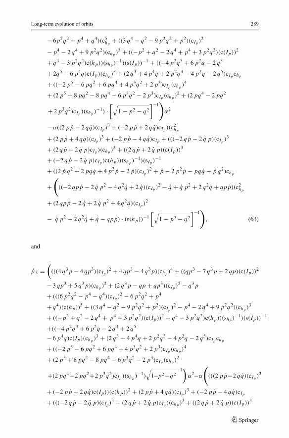
Long-term evolution of orbits 289
− 6p2q2 + p4 + q4)(c5hp
+ ((3 q4 − q2 − 9 p2q2 + p2)(cIp )2
−p4 − 2 q4 + 9 p2q2)(chp )3 + ((−p2 + q2 − 2 q4 + p4 + 3 p2q2)(c(Ip))2
+ q4 − 3 p2q2)c(hp))(shp )−1)(s(Ip))−1 + ((−4 p2q3 + 6 p2q − 2 q3
+ 2q5 − 6 p4q)c(Ip)(chp )3 + (2 q3 + 4 p4q + 2 p2q3 − 4 p2q − 2 q5)cIp chp
+ ((−2 p5 − 6 pq2 + 6 pq4 + 4 p3q2 + 2 p3)cIp (chp )4
+ (2 p5 + 8 pq2 − 8 pq4 − 6 p3q2 − 2 p3)cIp (chp )2 + (2 pq4 − 2 pq2
+ 2 p3q2)cIp )(shp )−1) ·[√
1 − p2 − q2
]−1)
α2
−α((2 pp − 2 qq)(cIp )3 + (−2 pp + 2 qq)cIp )(c2hp
+ (2 pp + 4 qq)(cIp )3 + (−2 pp − 4 qq)cIp + (((−2 qp − 2 q p)(cIp )3
+ (2 qp + 2 q p)cIp )(chp )3 + ((2 qp + 2 q p)(c(Ip))3
+ (−2 qp − 2 q p)cIp )c(hp))(shp )−1)(sIp )−1
+ ((2 p q2 + 2 pqq + 4 p2p − 2 p)(cIp )2 + p − 2 p2p − pqq − p q2)chp
+(
((−2 qpp − 2 q p2 − 4 q2q + 2 q)(cIp )2 − q + q p2 + 2 q2q + qpp)(c2hp
+ (2 qpp − 2 q + 2 q p2 + 4 q2q)(cIp )2
− q p2 − 2 q2q + q − qpp) · (s(hp))−1[√
1 − p2 − q2
]−1)
, (63)
and
µ3 =(
(((4 q3p − 4 qp3)(cIp )2 + 4 qp3 − 4 q3p)(chp )4 + ((qp3 − 7 q3p + 2 qp)(c(Ip))2
− 3 qp3 + 5 q3p)(chp )2 + (2 q3p − qp + qp3)(cIp )2 − q3p
+ (((6 p2q2 − p4 − q4)(cIp )2 − 6 p2q2 + p4
+ q4)(c(hp))5 + ((3 q4 − q2 − 9 p2q2 + p2)(cIp )2 − p4 − 2 q4 + 9 p2q2)(chp )3
+ ((−p2 + q2 − 2 q4 + p4 + 3 p2q2)(c(Ip))2 + q4 − 3 p2q2)c(hp))(shp )−1)(s(Ip))−1
+((−4 p2q3 + 6 p2q − 2 q3 + 2 q5
− 6 p4q)c(Ip)(chp )3 + (2 q3 + 4 p4q + 2 p2q3 − 4 p2q − 2 q5)cIp chp
+ ((−2 p5 − 6 pq2 + 6 pq4 + 4 p3q2 + 2 p3)cIp (chp )4
+ (2 p5 + 8 pq2 − 8 pq4 − 6 p3q2 − 2 p3)cIp (chp )2
+(2 pq4−2 pq2+2 p3q2)cIp )(shp )−1)
√1−p2−q2
−1)α2−α
(
(((2 pp−2 qq)(cIp )3
+ (−2 pp + 2 qq)c(Ip))(c(hp))2 + (2 pp + 4 qq)(cIp )3 + (−2 pp − 4 qq)cIp
+ (((−2 qp − 2 q p)(cIp )3 + (2 qp + 2 q p)cIp )(chp )3 + ((2 qp + 2 q p)(c(Ip))3
123
290 P. Gurfil et al.
+ (−2 qp − 2 q p)cIp )c(hp))(shp )−1)(sIp )−1 + (((2 p q2 + 2 pqq + 4 p2p
− 2p)(cIp )2 + p − 2p2p−pqq
− pq2)chp +(((−2 qpp−2 q p2−4 q2q+2 q)(c(Ip))2−q+q p2+2 q2q
+ qpp)(chp )2+(2 qpp−2 q+2 q p2+4 q2q)(cIp )2−q p2
−2 q2q+q−qpp)(shp )−1) ·[√
1 − p2 − q2
]−1)
(64)
Appendix B: Niching genetic algorithms
The most commonly used Genetic Algorithm (GA) is the so-called “Simple GA” (Goldberg1989). To perform an evolutionary search, the Simple GA uses the operators of crossover,reproduction, and mutation. A crossover is used to create new solution strings (“children”or “offspring”) from the existing strings (“parents”). Reproduction copies individual stringsaccording to the objective function values. Mutation is an occasional random alteration ofthe value of a string position, used to promote diversity of solutions.
Although Simple GA’s are capable of detecting the global optimum, they suffer fromtwo main drawbacks. First, convergence to a local optimum is possible due to the effect ofpremature convergence, where all individuals in a population become nearly identical beforethe optima has been located. Second, convergence to a single optimum does not revealother optima, which may exhibit attractive features. To overcome these problems, modifi-cations of Simple GA’s were considered. These modifications are called niching methods,and are aimed at promoting a diversity of solutions for multi-modal optimisation problems.In other words, instead of converging to a single (possibly local) optimum, niching allowsfor a number of optimal solutions to co-exist, and it lets the designer choose the appropri-ate one. The niching method used throughout this study is that of Deterministic Crowding.According to this method, individuals are first randomly grouped into parent pairs. Each pairgenerates two children by application of the standard genetic operators. Every child thencompetes against one of his parents. The winner of the competition moves on to the nextgeneration. By using the notation Pi for a parent, Ci for a child, f (·) for a fitness, and d(·)for a distance, a pseudo-code for the two possible parent-child tournaments can be writtenas follows (Gurfil and Kasdin 2002a, b):
If [d(P1, C1) + d(P2, C2) = d(P1, C2) + d(P2, C1)]If f (C1) ≥ f (P1) replace P1 with C1
If f (C2) ≥ f (P2) replace P2 with C2
ElseIf f (C1) ≥ f (P2) replace P2 with C1
If f (C2) ≥ f (P1) replace P1 with C2
In addition to applying the Deterministic Crowding niching method, we used a two-pointcrossover instead of a single-point one. In the Simple GA, the crossover operator breaksthe binary string of parameters, the “chromosome,” at a random point and exchanges thetwo pieces to create a new “chromosome.” In a two-point crossover, the “chromosome” isrepresented with a ring. The string between the two-crossover points is then exchanged. Thetwo-point crossover or other multiple-point crossover schemes have preferable propertieswhen optimisation highly nonlinear functions is performed.
123
Long-term evolution of orbits 291
References
Bills, B.G.: Non-chaotic obliquity variations of Mars. The 37th Annual Lunar and Planetary Science Confer-ence, pp. 13–17, March 2006, League City, TX (2006)
Brouwer, D.: Solution of the problem of artificial satellite theory without drag. Astron. J. 64, 378–397 (1959)Brouwer, D., van Woerkom, A.J.J.: The secular variations of the orbital elements of the principal planets.
Astronomical papers prepared for the use of the American Ephemeris and Nautical Almanac, vol. 13,Part 2, pp. 81–107. US Government Printing Office, Washington, DC (1950)
Brumberg, V.A., Evdokimova, L.S., Kochina, N.G.: Analytical methods for the orbits of artificial satellites ofthe moon. Celestial Mech. 3, 197–221 (1971)
Burns, J.: Dynamical characteristics of phobos and deimos. Rev. Geophys. Space Phys. 6, 463–483 (1972)Burns, J.: The dynamical evolution and origin of the Martian moons. Vistas Astron. 22, 193–210 (1978)Colombo, G.: Cassini’s second and third laws. Astron. J. 71, 891–896 (1966)Cook, G.E.: Luni-solar perturbations of the orbit of an earth satellite. Geophys. J. 6(3), 271–291 (1962)Efroimsky, M., Goldreich, P.: Gauge freedom in the N-body problem of celestial mechanics. Astron. Astrophys.
415, 1187–1199, astro-ph/0307130 (2004)Efroimsky, M.: Long-term evolution of orbits about a precessing oblate planet. 1. The case of uniform
precession. astro-ph/0408168 (2004) [This preprint is a very extended version of Efroimsky (2005)]Efroimsky, M.: Long-term evolution of orbits about a precessing oblate planet: 1. The case of uniform pre-
cession. Celestial Mech. Dynam. Astron. 91, 75–108 (2005)Efroimsky, M.: Long-term evolution of orbits about a precessing oblate planet: 2. The case of variable
precession. Celestial Mech. Dynam. Astron. 96, 259–288 (2006a)Efroimsky, M.: Long-term evolution of orbits about a precessing oblate planet: 2. The case of variable
precession. astro-ph/0607522 (2006b) [This preprint is a very extended version of Efroimsky (2006a)]Efroimsky, M.: Gauge freedom in orbital mechanics. Ann. N. Y. Academy Sci. 1065, 346–374, astro-
ph/0603092 (2006c)Efroimsky, M., Lainey, V.: The physics of bodily tides in terrestrial planets, and the appropriate scales of
dynamical evolution. J. Geophys. Res.—Planets (2007, in press)Everhart, E.: An efficient integrator that uses Gauss-Radau spacings. Dynamics of comets: their origin and
evolution. In: Carusi, A., Valsecchi, G.B. (eds.) Proceedings of IAU Colloquium 83 held in Rome on11–15 June 1984. vol. 115, p. 185. Astrophysics and Space Science Library, Dordrecht, Reidel (1985)
Goldberg, D.E.: Genetic Algorithms in Search, Optimization and Machine Learning. Addison-Wesley,Reading, MA (1989)
Goldreich, P.: Inclination of satellite orbits about an oblate precessing planet. Astron. J. 70, 5–9 (1965)Gurfil, P., Kasdin, N.J., Arrell, R.J., Seager, S., Nissanke, S.: Infrared space observatories: How to mitigate
zodiacal dust interference. Astrophys. J. 567, 1250–1261 (2002)Gurfil, P., Kasdin, N.J.: Characterization and design of out-of-ecliptic trajectories using deterministic crowding
genetic algorithms. Comput. Methods Appl. Mech. Eng. 191, 2169–2186 (2002a)Gurfil, P., Kasdin, N.J.: Niching genetic algorithms-based characterization of geocentric orbits in the 3D
elliptic restricted three-body problem. Comput. Methods Appl. Mech. Eng. 191, 5673–5696 (2002b)Hartmann, W.K.: Martian cratering 9: toward resolution of the controversy about small craters. Icarus 189,
274–278 (2007)Innanen, K.A., Zheng, J.Q., Mikkola, S., Valtonen, M.J.: The Kozai Mechanism and the stability of planetary
orbits in binary star systems. Astron. J. 113, 1915–1919 (1997)Kilgore, T.R., Burns, J.A., Pollack, J.B.: Orbital evolution of “Phobos” following its “capture”. Bull. Am.
Astron. Soc. 10, 593 (1978)Kozai, Y.: On the effects of the Sun and the Moon upon the motion of a close Earth satellite. SAO Special
Report 22, 7–10 (1959)Kozai, Y.: Effect of precession and nutation on the orbital elements of a close earth satellite. Astron. J. 65,
621–623 (1960)Lainey, V., Duriez, L., Vienne, A.: New accurate ephemerides for the Galilean satellites of Jupiter. I. Numerical
integration of elaborated equations of motion. Astron. Astrophys. 420, 1171–1183 (2004)Lainey, V., Gurfil, P., Efroimsky, M.: Long-term evolution of orbits about a precessing oblate planet: 4.
A comprehensive model (2008 in preparation)Laskar, J.: Secular evolution of the solar system over 10 million years. Astron. Astrophys. 198, 341–362 (1988)Laskar, J., Robutel, J.: The chaotic obliquity of the planets. Nature 361, 608–612 (1993)Murison, M.: Satellite Capture and the Restricted Three-Body Problem. Ph.D. Thesis, University of Wisconsin,
Madison (1988)Nesvorný, D., Vokrouhlický, D.: Analytic theory of the YORP effect for near-spherical objects. Astron.
J. 134, 1750–1768 (2007)
123
292 P. Gurfil et al.
Paige, D.A., Golombek, M.P., Maki, J.N., Parker, T.J., Crumpler, L.S., Grant, J.A., Williams, J.P.: MER small-crater statistics: evidence against recent quasi-periodic climate variations. Seventh Int. Conference Mars,9–13 July 2007, Caltech, Pasadena, CA (2007)
Pang, K.D., Pollack, J.B., Veverka, J., Lane, A.L., Ajello, J.M.: The composition of phobos: evidence forcarbonateous chondrite surface from spectral analysis. Science 199, 64 (1978)
Pollack, J.B., Burns, J.A., Tauber, M.E.: Gas drag in primordial circumplanetary envelopes. a mechanism forsatellite capture. Icarus 37, 587 (1979)
Proskurin, V.F., Batrakov, Y.V.: Perturbations of the motion of artificial satellites, caused by the earth oblate-ness. Bull. Inst. Theor. Astro. 7, 537–548 (1960)
Smith, D.E., Lemoine, F.G., Zuber, M.T.: Simultaneous estimation of the masses of mars, phobos, and deimosusing spacecraft distant encounters. Geophys. Res. Lett. 22, 2171–2174 (1995)
Szebehely, V.: Theory of Orbits. Academic Press, NY (1967)Tolson, R.H., 15, collaborators.: Viking first encounter of phobos. Preliminary results. Science 199, 61 (1978)Touma, J., Wisdom, J.: The chaotic obliquity of Mars. Science 259, 1294–1297 (1993)Touma, J., Wisdom, J.: Lie-Poisson integrators for rigid body dynamics in the solar system. Astron.
J. 107, 1189–1202 (1994)Veverka, J.: Phobos and deimos. Sci. Am. 236, 30 (1977)Ward, W.: Large-scale variations in the obliquity of Mars. Science 181, 260–262 (1973)Ward, W.: Climatic variations of Mars. Astronomical theory of insolation. J. Geophys. Res. 79, 3375–
3386 (1974)Ward, W.: Present obliquity oscillations of Mars—Fourth-order accuracy in orbital e and i. J. Geophys.
Res. 84, 237–241 (1979)Ward, W.: Comments on the long-term stability of the earth’s obliquity. Icarus 50, 444–448 (1982)Zhang K., Hamilton, D.P.: Dynamics of inner neptunian satellites. Abstracts of the 37th DPS Meeting of the
Americal Astronomical Society. In: AAS Bulletin, 37, 667–668 (2005)Waz, P.: Analytical theory of the motion of phobos: a comparison with numerical integration. Astron. Astro-
phys. 416, 1187–1192 (2004)
123