longer-run evidence on whether building energy codes...

Longer-Run Evidence on Whether Building

Energy Codes Reduce Residential

Energy Consumption

Matthew J. Kotchen

Abstract: This paper provides an ex post evaluation of how changes to a buildingenergy code affect energy consumption. Using residential billing data for electricity andnatural gas over 11 years, the analysis is based on comparisons between residences con-structed just before and just after a building code change in Florida. While an earlierstudy using 3 years of data for the same residences showed savings for both electricityand natural gas, new results show an enduring savings for natural gas only. These find-ings underscore the importance of accounting for all sources of energy consumptionwhen conducting evaluations of building codes. More broadly, the results provide acounterpoint to the growing literature casting doubt on whether ex ante forecasts ofenergy efficiency policies and investments can provide useful information about actualenergy savings. Indeed, more than a decade after Florida’s energy code change, the mea-sured energy savings still meets or exceeds the forecasted amount.

JEL Codes: Q47, Q48

Keywords: Building codes, Energy, Evaluation, Regulation

ARE BUILDING ENERGY CODES effective at saving energy? The answer to this ques-tion is important given the growing reliance on building codes as a central part of energyand climate policy in the United States and abroad. The promotion of building energycodes is a priority at the US Department of Energy, which estimates energy expendi-ture savings in the hundreds of billions of dollars by 2030, with emission reductionsequivalent to taking millions of vehicles off the road (US DOE 2011). In the Euro-pean Union, all member countries must comply with the revised Energy Performance

Matthew Kotchen is at Yale University and the National Bureau of Economic Research([email protected]). Without implicating them for any errors or omissions, I amgrateful to Grant Jacobsen, Arik Levinson, Erin Mansur, and Joe Shapiro for helpful commentsand discussion. I also thank two anonymous reviewers and the editor Stephen Holland for con-structive suggestions on an earlier version of the paper.

Received February 15, 2016; Accepted June 1, 2016; Published online January 25, 2017.

JAERE, volume 4, number 1. © 2017 by The Association of Environmental and Resource Economists.All rights reserved. 2333-5955/2017/0401-0004$10.00 http://dx.doi.org/10.1086/689703

135

This content downloaded from 130.132.173.190 on September 12, 2017 09:22:33 AMAll use subject to University of Chicago Press Terms and Conditions (http://www.journals.uchicago.edu/t-and-c).

136 Journal of the Association of Environmental and Resource Economists March 2017

of Buildings Directive that seeks to promote energy efficiency and help meet the EU’sgreenhouse gas emissions targets (EuropeanUnion 2012). Despite the growing empha-sis on building codes as a regulatory instrument, our understanding of the actual im-pacts on energy consumption remains thin. There are only a handful of peer reviewedstudies that seek to evaluate the extent to which building energy codes affect construc-tion practices and energy consumption, and among these studies the results are quitemixed.1

In one of the more recent papers, Jacobsen and Kotchen (2013) study the effectsof a change in Florida’s building code using residential billing data for electricity andnatural gas. Their study is based on a comparison between residences in Gainesville,Florida, that were constructed just before and just after an increase in the stringencyof Florida’s energy code in 2002. Jacobsen and Kotchen find that the code change causeda 4% decrease in electricity consumption and a 6% decrease in natural gas consump-tion, and these savings were close to those predicted ex ante for the code change. Theyalso find that energy consumption in post-code change residences is less responsiveto weather shocks in ways consistent with greater energy efficiency and that the socialand private payback periods for code compliance range between 3.5 and 6.4 years, re-spectively.

Even more recently, Levinson (2014) studies the effect of building energy codes onelectricity consumption in California. Despite the fact that California is often perceivedas a model state promoting energy-efficient buildings, Levinson (2014) finds little ev-idence that building codes have anything close to the anticipated effect on residentialelectricity consumption.2 An important aspect of Levinson’s contribution is the carefulattention given to building age as a distinct feature from building vintage with respectto codes. He shows that newer homes consume less electricity simply because they arenew, and this observation can be problematic for reliably estimating the effect of build-ing codes. Hence careful methods are needed to separate age from vintage effects, thatis, older and newer homes from those built before or after a building code change.

The potential importance of a newness effect raises questions about Jacobsen andKotchen’s research design and findings in Florida. Did the post-code-change residencesconsume less energy simply because they were new? And, over time, will the energy con-sumption of post-code-change residences more closely resemble the pre-code-changeresidences as the differences in age reflect less of a newness effect? Indeed, Levinson(2014, 8) writes, “I suspect if we revisited those Gainesville homes today, 10 years later,

1. Studies that focus explicitly on the effects of regulatory building codes include Horowitzand Haeri (1990), Jaffe and Stavins (1995), Aroonruengsawat et al. (2012), Costa and Kahn(2010), Jacobsen and Kotchen (2013), and Levinson (2014).

2. Levinson’s (2014) paper has received a substantial amount of media attention given its coun-terintuitive finding. Readers may find of interest a 30-minute Freakonomics podcast dedicated tothe paper at http://freakonomics.com/tag/arik-levinson/.


Building Energy Codes and Residential Consumption Kotchen 137

we would find no difference in energy use for households built before and after the 2002code change.”

This conjecture is the starting point for the present paper. I test whether Jacobsenand Kotchen’s findings still hold 11 years after the building code change. This is im-portant for at least two reasons. First, Jacobsen and Kotchen’s approach provides a clearidentification strategy for estimating building code effects, and their results are some ofthe very few that find an effect. Knowing whether the results endure is therefore highlypolicy relevant. Second, regarding energy efficiency investments more generally, a grow-ing literature finds that ex ante engineering studies significantly overestimate realized sav-ings in ex post evaluations.3 Yet Jacobsen and Kotchen’s study provides a counterpointin the important context of building codes. Because they find that the engineering fore-casts are in line with the estimated savings, the question is whether or not the resultshold up.

This paper also contributes with new insight about the effect of building codes onenergy consumption over time and how future studies should approach ex post eval-uations. The results do not yield a simple yes or no to an enduring building code effect.There are differences between the results for electricity and natural gas. While the ini-tial estimates of the building code effect on electricity consumption diminish over time,the original results for natural gas underestimate the longer-term energy savings. Never-theless, the overall net effect on energy consumption in a combined measure of millionBritish thermal units indicates a rather consistent level of code-induced energy savingsover the 11-year period. Together, the results highlight the importance of not focusingexclusively on electricity consumption—as most studies have done—and for waiting afew years after an energy code change to begin evaluation.

1. EMPIRICAL SETTING AND DATA COLLECTION

Florida’s residential building code that took effect in March 2002 included provisionsto strengthen the energy efficiency of newly constructed houses. The new requirementsfocused on energy used for space heating, space cooling, and water heating.4 To eval-uate the effect of the code on residential energy consumption, Jacobsen and Kotchenuse monthly billing data on electricity and natural gas consumption for residences inGainesville, Florida. They focus on residences constructed 3 years before and 3 yearsafter the building code change. A unique feature of their data set is that billing data werecombined with information about the physical characteristics of each residence, in addi-tion to monthly weather data.

3. Examples include Dubin, Meidema, and Chandran (1986), Metcalf and Hassett (1999),and Fowlie, Greenstone, and Wolfram (2015). The general issues are also reviewed in Allcottand Greenstone (2012), Gillingham and Palmer (2014), and Gerarden et al. (2015).

4. See Jacobsen and Kotchen (2013) for a detailed description of specific changes to the2002 code and methods of compliance.



Figure 1 illustrates the basic research design, the original data set, and the ex-panded data set used in the present paper. Before code change residences (BCCRs)were built in the years 1999–2001, and after code change residences (ACCRs) werebuilt in the years 2003–5.5 Unless otherwise indicated, residences built in 2002 areexcluded from the analysis because they cannot be clearly identified as having been sub-ject to the before or after code change requirements. Jacobsen and Kotchen used billingdata for the years 2004–6 to test for differences in energy consumption between thebefore and after code change residences. In this paper, I use an expanded data set thatincludes billing and weather data for the additional years 2007–14, yielding a totalof 11 years of energy consumption data after the building code change. Importantly,the additional billing data are for the identical set of before and after code change res-idences.

Most of the expanded data are from the same sources. Billing data were obtainedfrom Gainesville-green.com, and weather data on monthly average cooling degree days(ACDD) and average heating degree days (AHDD) were obtained for the weather sta-tion located at the Gainesville Regional Airport.6 The new data were merged with theoriginal to form a monthly panel from January 2004 through December 2014 for 2,239

Figure 1. Before and after code change residences, and the original and expanded data set

5. Residences are partitioned as BCCRs or ACCRs based on the observed effective year built(EYB) as it relates to the timing of energy code compliance at the time the residence received itspermits (for further details, see Jacobsen and Kotchen 2013). To ensure that only newly con-structed residences are included, any residence is dropped from the analysis if it had a utility billon record prior to the EYB, as this would indicate remodeling rather than new construction.

6. One difference in the source of data was necessary because natural gas data were not fullyup to date at Gainesville-green.com. I obtained natural gas billing data from October 2013through December 2014 directly from the Gainesville Regional Utilities (GRU), which makesall billing data publicly available for the two most recent years and ultimately provides thesource for updating Gainesville-green.com.


7. Two areas of missing billing data are for the majority of residences between April 2007and February 2008, and natural gas data for all residences in July 2014. Attempts to obtain themissing data from GRU have been unsuccessful. In what follows, I include all of the availabledata in the analysis, but all results are robust to dropping the months where there are missingdata.

8. Summary statistics for residence characteristics remain unchanged from Jacobsen andKotchen’s original analysis (see Jacobsen and Kotchen 2013, tables 1, 2). The only differencewith a potentially meaningful magnitude and statistical significance is that ACCRs are 4.5%smaller.


This content downloaded from 130.132.173.190 on September 12, 2017 09:22:33 AMAll use subject to University of Chicago Press Terms and Conditions (http://www.journals.uchicago.

residences, of which there are 1,293 BCCRs and 946 ACCRs.7 The time-invariantvariables on the physical characteristics of each residence are square footage; numberof bathrooms, bedrooms, and floors; and indicators for central air conditioning and ashingled roof.8

The top panel of figure 2 shows the average monthly electricity and natural gas con-sumption for all residences from January 2004 through December 2014. The hottermonths of the year—May through October—are shaded in the figure. There is a clearpattern where electricity consumption is higher during the summer months when de-

Figure 2. Average monthly electricity and natural gas consumption and cooling and heatingdegree days from 2004 to 2014, with months May–October shaded each year.

edu/t-and-c).


mand for air conditioning is greater, and natural gas consumption is higher duringwinter months when demand for heating is greater. The bottom panel of figure 2shows the patterns of monthly ACDD and AHDD based on the standard 65° Fahr-enheit threshold. Comparisons between the panels of figure 2 reveal how electricitydemand closely follows cooling degree days, while natural gas follows heating degreedays.

2. BEFORE AND AFTER CODE CHANGE COMPARISONS

2.1. Overall Differences

The key estimates from Jacobsen and Kotchen are regression-based, average differ-ences in electricity and natural gas consumption between before and after code changeresidences. The preferred specification is

Yijt 5 dCodeChangei 1 bXi 1 vjt 1 εijt, (1)

where the dependent variable represents consumption of either electricity (kilowatthours, kWhs) or natural gas (therms) in residence i, zip code j, and month t; CodeChangeiis an indicator for whether a residence was built after the code change; Xi is a vectorof the observable residence characteristics; vjt represents zip code by month-year fixedeffects; and εijt is an error term. The residence characteristics included in the model arethe natural log of square footage, an indicator for central air conditioning, an indi-cator for a shingled roof, and categorical variables for the number of bathrooms, bed-rooms, and stories.9 When reporting results for this model, and all others throughoutthe paper, I use standard errors that are clustered at the residence level.10

Table 1 reproduces Jacobsen and Kotchen’s results with the original 2004–6 datafor electricity and natural gas in the first column. I report the coefficients of interest,the δ’s, along with the mean monthly consumption and percentage difference betweenbefore- and after-code-change residences. Jacobsen and Kotchen found that ACCRsconsumed 4.27% less electricity and 6.67% less natural gas. The second column of ta-ble 1 reports analogous results using the expanded data set through 2014. With thelonger span of data, the difference in electricity consumption between before- and after-code-change residences is no longer statistically significant and has a point estimatevery close to zero. Levinson’s (2014) conjecture is therefore consistent with the datafor electricity; however, the pattern is very different for natural gas. The difference innatural gas consumption between before- and after-code-change residences for the ini-

9. Jacobsen and Kotchen also estimate models that include simply month-year fixed effects.Unless otherwise indicated, I focus throughout this paper on models with zip code by month-year fixed effects because they are less restrictive and therefore preferred.

10. In an appendix, available online, I discuss alternative specifications to estimate overallbuilding code differences that account explicitly for residence age. I report selected results andexplain why the models are not the preferred specifications for this particular analysis.



tial 2004–6 period provides an underestimate of the difference over the whole periodthrough 2014. Using the full series of data, I find that ACCRs use 13.5% less nat-ural gas on average—double the initial estimate, and with a high level of statistical sig-nificance.

The bottom panel of table 1 reports the results of new models that combine elec-tricity and natural gas into a single measure of overall energy consumption, quantifiedas millions of British thermal units (mmBtu).11 Combining electricity and natural gasinto a single measure of energy consumption has the advantage of estimating an over-all effect that accounts for potential substitution between energy sources. The focuson overall energy use is also more appropriate for a performance-based code, such asFlorida’s, where builders can trade off among different energy options. Because com-

11. The

All use subj

Table 1. Average Differences in Energy Consumption between Before-and After-Code-Change Residences

Original 2004–6 All Data 2004–14

Electricity:Code change –48.922*** –.502

(20.295) (15.651)Mean kWh/month 1,146.4 1,049.1Percent difference –4.27% –.05%Observations 64,471 256,635

Natural gas:Code change –1.572** –2.875***

(.704) (.537)Mean therms/month 23.6 21.3Percent difference –6.67% –13.5%Observations 64,471 254,467

Combined mmBtu:Code change –.324*** –.290***

(.109) (.080)Mean mmBtu/month 6.3 5.7Percent difference –5.14% –5.09%Observations 64,471 254,467

exact conversion is based on

This content downloaded fromect to University of Chicago Pre

mmBtu 5 0.0034121

130.132.173.190 on Sess Terms and Condition

Note. Each coefficient is from a different regression model that includes res-idence characteristics and zip code × month-year fixed effects. Standard errors inparentheses are clustered at the residence level.

* p < .10.** p < .05.*** p < .01.

416 × kWhs 1 0.1 × therms.

ptember 12, 2017 09:22:33 AMs (http://www.journals.uchicago.edu/t-and-c).


pliance is based on an overall rating, rather than conforming to specific requirements,there is no reason to expect that consumption of both electricity and natural gaswould necessarily decrease. These results indicate that for the initial period of 2004–6,ACCRs consume 5.14% less energy overall, and the difference is highly statisticallysignificant. Then, when using all the data through 2014, the average difference remainsnearly identical, at 5.09% with the same level of statistical significance.

The focus here is on energy consumption because building energy codes have sav-ing energy as the primary objective. But other outcomes are of interest as well, such ascost savings and carbon dioxide (CO2) emissions. Combining electricity and natural gasconsumption into mmBTUs is essentially a weighting between the two sources of res-idential energy use. Combining consumption into monthly energy expenditures and CO2

are alternative approaches that I consider to estimate overall average differences be-tween BCCRs and ACCRs.12

Table 2 reports the key coefficients from estimating (1) with the different depen-dent variables and all of the data from 2004 to 2014. The percentage changes in ex-penditures for electricity and natural gas are very close to the estimates for the changein consumption. They differ only because the rate schedules are nonlinear. The CO2

emissions are, however, a linear function of consumption, so these percentage changesare identical to those in table 1. The combined estimates for expenditures and emis-sions have a lower magnitude than those for consumption and are not statistically dif-ferent from zero. This difference occurs because the expenditure and emission weight-ing places relatively more weight on electricity than the weighting for mmBTU. Hence,while there is statistically significant evidence of energy savings, the evidence is weakerfor savings on utility bills and reducing CO2 emissions.

2.2. Differences by Effective Year Built

The previous estimates are for overall differences in energy consumption between BCCRsand ACCRs. As shown in figure 1, residences are partitioned into the two groups bytheir effective year built (EYB). The overall estimate can therefore be decomposed fur-ther into average differences by EYB. This is useful for examining potential differences

12. Expenditures are estimated based on GRU’s variable, pre-tax price schedules in 2014.After several attempts, I was not able to obtain price schedules for all years, but I have beenassured that prices did not change significantly over the 10-year period. Hence using 2014prices should provide reasonable estimates. For electricity, the increasing block rate is$0.031 for 0–250 kWh, $0.042 for 251–750 kWh, and $0.084 for over 750 kWh, along with$0.078 for all kWh as a fuel adjustment charge. For natural gas, the rate is $.502 per therm,plus a gas plant recovery charge of $0.0556 and a $0.46 fuel adjustment per therm. CO2 emis-sions for electricity are based on the marginal emission rate of electricity from Graff Zivin,Kotchen, and Mansur (2014) of 1.29 lbs/kWh for the FRCCNERC region, while for naturalgas it is the physical relationship of 11.7 lbs/therm.



in energy consumption by the age of residences within and between the two groups.Specifically, the model is

Yijt 5 dEYBi 1 bXi 1 vjt 1 εijt, (2)

which differs from (1) because EYBi is a categorical variable for each effective yearbuilt from 1999 through 2005. Jacobsen and Kotchen estimate the same model, andas in the original analysis, I include residences built in 2002 as the omitted category.

Figure 3 illustrates the estimated δ’s graphically for electricity, natural gas, and com-bined energy consumption. There is no trend in electricity consumption by effectiveyear built. This result is consistent with no observable, enduring effect of the energycode change on electricity consumption. With natural gas, however, the results are againdifferent. While there is no trend for the BCCRs, consumption is declining for theACCRs. Yet it appears that it may take a year or so for the decline to begin after thecode change, raising the possibility that residences with an effective year built in 2003(and maybe some in 2004) might still have been subject to the before-code-change

TAll use subject

Table 2. Average Differences in Variable Energy Expendituresand CO2 Emissions between Before- and After-Code-ChangeResidences

Expenditures CO2 Emissions

Electricity:Code change –.066 –.648

(2.433) (20.190)Monthly mean 140.1 1,353.4Percent difference –.05% –.05%

Natural gas:Code change –2.926*** –33.636***

(.547) (6.288)Monthly mean 21.7 249.0Percent difference –13.4% –13.5%

Combined:Code change –3.022 –34.545

(2.553) (21.811)Monthly mean 161.3 1,599.2Percent difference –1.87% –2.2%

his content downloaded from 1 to University of Chicago Press

30.132.173.190 on Se Terms and Conditions

Note. Each coefficient is from a different regression model that in-cludes residence characteristics and zip code × month-year fixed effects.Models have the same number of observations as those indicated in table 1.Standard errors in parentheses are clustered at the residence level.

* p < .10.** p < .05.*** p < .01.

ptember 12, 2017 09:22:33 AM (http://www.journals.uchicago.edu/t-and-c).

13. Jacobsen and Kotchen’s figures 3 and 4 present results for electricity and natural gas us-ing only the first 3 years of consumption data. Those reported here differ by clearly showing nocode change effect on electricity, but a more clear effect on natural gas. Jacobsen and Kotchendid not provide separate estimates for combined energy consumption.



requirements. The results for combined energy consumption, which is effectively aweighted average of electricity and natural gas, more closely resemble those for nat-ural gas. The important takeaway from the figure is that the trend in energy consump-tion appears to break around the time of the energy code change, suggesting that thecode change had an effect on energy consumption, rather than the estimates simplycapturing an age effect.13

2.3. Yearly Differences

While the energy code change is associated with lower energy consumption overall,as measured with mmBtu, the results in table 1 clearly indicate that something differ-ent is happening over time with electricity compared to natural gas. This motivatescloser scrutiny of how the estimated building code effects differ over time. Accord-ingly, I estimate additional models of the form

Figure 3. Overall differences in electricity, natural gas, and combined energy consumptionamong residences by effective year built, relative to those built in 2002, with 95% confidenceintervals.

edu/t-and-c).


Yijt 5 dCodeChangei × Yeart 1 bXi 1 vjt 1 εijt, (3)

where Yeart is a categorical variable for each year in the sample. Estimation of thismodel yields distinct energy code effects for each year, where the δ’s capture differ-ences in the annual averages between BCCRs and ACCRs. I estimate separate mod-els for electricity, natural gas, and mmBtu and report the results graphically.

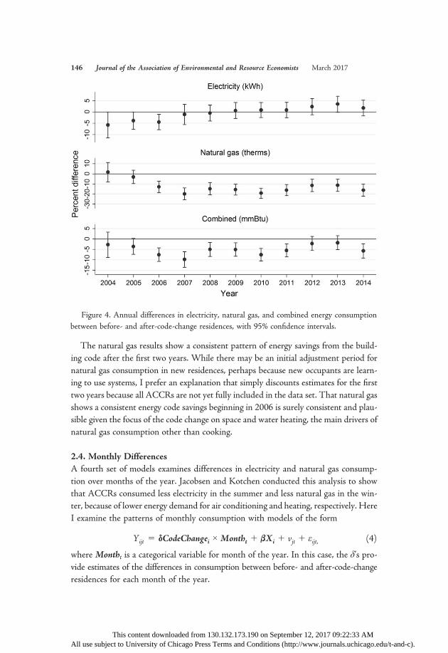
Figure 4 includes all three sets of results. The δ’s are scaled as a percentage dif-ference from average consumption for the corresponding energy measure and year. Itis worth keeping in mind that when the estimates are based on annual differences, thereis less statistical power, yet the trend in point estimates is of primary concern here. Theresults for electricity illustrate an upward trend and clearly show how focusing on thefirst three years of data provides an overestimate of the electricity savings.14 Indeed,ACCRs appear to consume even more electricity in the more recent years, despite ini-tially consuming less. But the trend clearly differs for natural gas. After the first twoyears, the ACCRs consume significantly less natural gas, with point estimates rangingbetween 10% and 20% less, and the difference endures over time. Finally, the resultsfor overall energy consumption indicate that ACCRs uniformly consume less energy,but the differences vary from year to year, with point estimates ranging between 2%and 10% less. In this case, we can see visually how the short-run estimate over threeyears is actually quite close to the 11-year estimate.

What might explain the pattern of differences for electricity and natural gas overthe 11-year period?With respect to electricity, Levinson (2014) posits that such a pat-tern might arise because ACCRs are simply newer, and the newness effect might dis-sipate over time. Although better insulated when newly constructed, residences mayquickly lose some of the tight envelope that increases initial efficiency. New heatingand cooling systems are more likely to have clean and efficient air filters that are sub-sequently changed less regularly. It may also take the occupants of new residences timeto fully move in and acquire the same set of appliances as those in older residences.

An alternative explanation for the electricity results is that, despite the small dif-ferences in the effective year built between BCCRs and ACCRs, occupants of theACCRs may be different, perhaps younger and more likely to add members to a grow-ing family. Younger families may also have relatively increasing demands for goods thatuse electricity in ways unaffected by the building code (e.g., televisions and electronics).In this case, however, the relative increase in electricity consumption in ACCRs overtime would not mean the code change had no effect. Instead, it would raise questionsabout the identification assumption underlying the regression models for estimatingaverage differences, a topic to which I return in section 3.

14. Recall that ACCRs are continuously entering the data set in 2004 and 2005. Estimatesfor these years are therefore based on a smaller set of ACCRs with monthly observations notuniformly spread over months of the year.




The natural gas results show a consistent pattern of energy savings from the build-ing code after the first two years. While there may be an initial adjustment period fornatural gas consumption in new residences, perhaps because new occupants are learn-ing to use systems, I prefer an explanation that simply discounts estimates for the firsttwo years because all ACCRs are not yet fully included in the data set. That natural gasshows a consistent energy code savings beginning in 2006 is surely consistent and plau-sible given the focus of the code change on space and water heating, the main drivers ofnatural gas consumption other than cooking.

2.4. Monthly Differences

A fourth set of models examines differences in electricity and natural gas consump-tion over months of the year. Jacobsen and Kotchen conducted this analysis to showthat ACCRs consumed less electricity in the summer and less natural gas in the win-ter, because of lower energy demand for air conditioning and heating, respectively. HereI examine the patterns of monthly consumption with models of the form

Yijt 5 dCodeChangei × Montht 1 bXi 1 vjt 1 εijt, (4)

where Montht is a categorical variable for month of the year. In this case, the δ’s pro-vide estimates of the differences in consumption between before- and after-code-changeresidences for each month of the year.

Figure 4. Annual differences in electricity, natural gas, and combined energy consumptionbetween before- and after-code-change residences, with 95% confidence intervals.

edu/t-and-c).


Figure 5 illustrates the results graphically for electricity and natural gas.15 I reportresults using the original 2004–6 data and the full set of data through 2014. The toppanel shows the pattern for electricity described by Jacobsen and Kotchen: using data3 years after the code change, there are no differences in electricity consumption be-tween before- and after-code-change residences during the colder and winter months,but the ACCRs consume less electricity during the hotter and summer months whendemand for air conditioning is greater.16 When using all the data through 2014, theprofile of electricity consumption remains the same, yet the difference between before-and after-code-change residences tends to be greater across all months of the year. Wehave already established in figure 4 that electricity consumption is increasing overtime in the ACCRs compared to the BCCRs, and figure 5 shows that the increase

Figure 5. Monthly differences in electricity and natural gas consumption between beforeand after code change residences, 2004–6 and all data through 2014, with 95% confidence in-tervals.

15. I do not report the results for mmBtu because the reason for estimating monthly differ-ences is to gain insight into the seasonal patterns of consumption for the original sources of en-ergy demand, electricity and natural gas. But, of course, similarly formatted results for mmBtuare available upon request.

16. The results presented here are based on models with zip code by month-year fixed ef-fects rather than simply month-year fixed effects as shown in Jacobsen and Kotchen’s figures 1and 2.



occurs because of greater baseline demand rather than a seasonal effect.17 The naturalgas results in the bottom panel reveal lower consumption of natural gas in ACCRsin the colder and winter months, indicating greater efficiency with heating. With nat-ural gas, however, there does not appear to be an increasing or decreasing trend overmonths of the year when using the full set of data, and this is consistent with theACCRs consuming uniformly less natural gas in figure 4.

3. DIFFERENCES IN WEATHER RESPONSIVENESS

An advantage of the analysis in the previous section is that it yields an estimate ofthe average effect of the building code change on residential energy consumption. A dis-advantage of the approach is potential vulnerability to omitted variable bias. If there issome unobserved variable that is correlated with energy consumption and the BCCR-ACCR categorization, for reasons unrelated to the building code change, then the esti-mates could be biased. As discussed previously, examples include differences in familiesthat purchased homes in Gainesville a few years later, and differences in the stock ofappliances in newer residences.

To address these concerns, I estimate models to test for differences in the wayBCCRs and ACCRs adjust energy consumption in response to weather shocks. Theapproach is essentially a difference-in-differences strategy that takes account of unob-servable, time-invariant heterogeneity with the inclusion of residence fixed effects.While Jacobsen and Kotchen estimate similarly specified fixed effects models for elec-tricity and natural gas consumption separately, I focus here on the combined measureof mmBtu.18 The combined measure is preferable because, as mentioned previously,it yields an overall effect that accounts for potential substitution between electricity andnatural gas.

The first model takes the form

Yit 5 dCodeChangei × ACDDt,AHDDt½ � 1 b ACDDt,AHDDt½ �1 Montht 1 Yeart 1 mi 1 εit,

(5)

where the dependent variable is monthly mmBtu consumption, the code change in-dicator is interacted with the weather variables,Montht is a set of month of year dum-

(5)

17. Although I do not find evidence for it here, a seasonal effect of comparatively increasingdemand for electricity in the summer by ACCRs would be consistent with an air conditioningrebound effect.

18. Though not reported here, I also estimated separate models for electricity and naturalgas. The specifications are identical to those in J&K’s analysis but with the expanded data setthrough 2014. The main results continue to hold, whereby ACCRs are less responsive in elec-tricity due to ACDD and less responsive in natural gas due to AHDD. These results are avail-able upon request.



mies, Yeart is a set of year dummies, and mi is a residence fixed effect. The model pro-vides estimates of how temperature variation affects monthly energy consumption inthe BCCRs (the b ’s) and how the estimates differ in the ACCRs (the δ’s).

Two other specifications provides alternative estimates of the difference in differ-ences—that is, the δ’s—but control for the direct weather effects more flexibly. Onespecification is

Yit 5 dCodeChangei × ACDDt,AHDDt½ � 1 vt 1 mi 1 εit, (6)

where vt represents month-year fixed effects. Note that the weather variables do notenter on their own because with one weather station, they are not separately identifiedfrom the month-year fixed effects. The other specification is the same except for the in-clusion of zip code by month-year fixed effects,, as specified in previous models.

Table 3 reports the results of all three models using all of the data through 2014.The results of specification (5), reported in the first column, show the unsurprisingresult that greater ACDD and AHDD in a month increases energy consumption.This is reflected in the positive and statistically significant estimates of bACDD and

All use

Table 3. Difference-In-Differences Estimates of Energy Consumption due toWeather Variability, 2004–14

mmBtu

(1) (2) (3)

Code change × ACDD (dACDD) –.014*** –.013*** –.009**(.004) (.004) (.004)

Code change × AHDD (dAHDD) –.118*** –.112*** –.093***(.011) (.011) (.010)

ACDD (bACDD) .115*** . . . . . .(.004)

AHDD (dAHDD) .403*** . . . . . .(.007)

Month dummies Yes No NoYear dummies Yes No NoMonth-year dummies No Yes NoZip code × month-year dummies No No YesResidence fixed effects Yes Yes YesR-squared (within) .273 .286 .331Observations 254,467 254,467 245,467

This content downloaded from 130.1 subject to University of Chicago Press Ter

32.173.190 on Sms and Conditio

eptember 12, 20ns (http://www.j

Note. Standard errors are clustered at the residence level.* p < .10.** p < .05.*** p < .01.

17 09:22:33 AMournals.uchicago.edu/t-and-c).


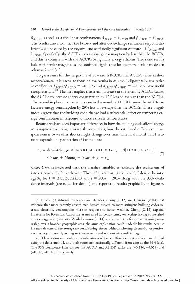
bAHDD, as well as a the linear combinations bACDD 1 dACDD and bAHDD 1 dAHDD.The results also show that the before- and after-code-change residences respond dif-ferently, as indicated by the negative and statistically significant estimates of dACDD anddAHDD. Specifically, the ACCRs increase energy consumption by less than the BCCRs,and this is consistent with the ACCRs being more energy efficient. The same resultshold with similar magnitudes and statistical significance for the more flexible models incolumns 2 and 3.19

To get a sense for the magnitude of how much BCCRs and ACCRs differ in theirresponsiveness, it is useful to focus on the results in column 1. Specifically, the ratiosof coefficients dACDD/bACDD 5 –0 : 123 and dAHDD/bAHDD 5 –0 : 292 have usefulinterpretations.20 The first implies that a unit increase in the monthly ACDD causesthe ACCRs to increase energy consumption by 12% less on average than the BCCRs.The second implies that a unit increase in the monthly AHDD causes the ACCRs toincrease energy consumption by 29% less on average than the BCCRs. These magni-tudes suggest that the building code change had a substantial effect on tempering en-ergy consumption in response to more extreme temperatures.

Because we have seen important differences in how the building code affects energyconsumption over time, it is worth considering how the estimated differences in re-sponsiveness to weather shocks might change over time. The final model that I esti-mate expands on specification (5) as follows:

Yit 5 dCodeChangei × ACDDt,AHDDt½ � × Yeart 1 b ACDDt,AHDDt½ �× Yeart 1 Montht 1 Yeart 1 mi 1 εit,

(7)

where Yeart is interacted with the weather variables to estimate the coefficients ofinterest separately for each year. Then, after estimating the model, I derive the ratiodkt/bkt for k 5 ACDD,AHDD and t 5 2004 ::: 2014 along with the 95% confi-dence intervals (see n. 20 for details) and report the results graphically in figure 6.

(7)

19. Studying California residences over decades, Chong (2012) and Levinson (2014) findevidence that more recently constructed houses subject to more stringent building codes in-crease electricity consumption more in response to hotter weather. Chong (2012) explainshis results for Riverside, California, as increased air conditioning ownership having outweighedother energy-saving impacts. While Levinson (2014) is able to control for air conditioning own-ership over a broader geographic area, the same explanation could underlie his results becausehis models control for average air conditioning effects without allowing electricity responsive-ness to vary differently among residences with and without air conditioning.

20. These ratios are nonlinear combinations of two coefficients. Test statistics are derivedusing the delta method, and both ratios are statistically different from zero at the 99% level.The 95% confidence intervals for the ACDD and AHDD ratios are (–0.186, –0.059) and(–0.340, –0.243), respectively.


21. The large confidence interval for the point estimate in 2007 is most likely the result ohaving fewer observations to estimate an effect for that year. Recall the missing data mentionedin n. 7.



Despite the very different empirical strategy from that in section 2, there is a nowfamiliar pattern to the results. Soon after the building code change, ACCRs increaseenergy consumption significantly less in response to more ACDD, and this suggestsgreater efficiency with air conditioning.21 But the difference between before- and after-code-change residences appears to dissipate over time, until there is no evidence ofan energy code affect about 8 years later. This pattern is clearly consistent with a relativenewness effect in ACCRs that is not enduring. In contrast, the difference in responsive-ness to AHDD appears roughly constant over the 11 years and is always statisticallydifferent from zero, with point estimates ranging between 20% and 30%. This result sug-gests that the energy code had real effects on the efficiency of residences for heating,and this tracks the previous findings for natural gas.

4. CONCLUSION

This paper considers the question of whether building energy codes actually save en-ergy. Using more than a decade’s worth of billing data for residences in Gainesville,

Figure 6. Annual difference in differences in energy consumption responsiveness betweenbefore- and after-code-change residences due to weather variability, with 95% confidence inter-vals.

f

edu/t-and-c).


Florida, the answer is yes, but the results differ for electricity and natural gas. De-spite what appears to be an initial code change effect that reduces electricity con-sumption, the difference between before- and after-code-change residences disap-pears after a few years. In contrast, the code change has a significant and enduringeffect on natural gas consumption, causing a reduction of more than 10%. Both theelectricity and natural gas results are consistent with the way before- and after-code-change residences respond to weather shocks. In particular, ACCRs increase naturalgas consumption by nearly 30% less than BCCRs in response to marginally colderweather.

Comparison of results from the present paper to those in Jacobsen and Kotchen’soriginal study yields two important methodological insights. First, future studies thattake advantage of the discontinuity design of comparing before- and after-code-changeresidences should wait several years after the code change before using billing datafor analysis. Second, evaluation of building codes should not focus exclusively on elec-tricity consumption, which has been the case in most previous studies. Energy codesseek to improve the efficiency of space heating, space cooling, and water heating.While natural gas is used primarily for these purposes, a growing share of residentialelectricity consumption is for other uses, including appliances, electronics, and televi-sions. There is also the potential for substitution among energy sources for home heatingand many appliances (e.g., clothes dryers and hot water heaters). Unfortunately dataon energy sources for different uses are not available for this study, but the estimates ofcombined energy consumption seek to account for such substitution. In addition to es-timating the overall energy effect, I consider the effect on energy expenditures and CO2

emissions, which are effectively different weighting approaches that place more empha-sis on electricity than natural gas. While there is statistically significant evidence of over-all energy savings, the evidence is weaker for savings on utility bills and reducing CO2

emissions.Finally, the results of this study have broader implications for the evaluation of en-

ergy efficiency policies. While a growing number of studies find that engineering fore-casts significantly overestimate realized savings of efficiency investments, this does notappear to be the case with Florida’s building code. Forecasts predicted that the 2002code change would translate into a 2% increase in residential energy efficiency. Therevised estimate here is very close to the forecast: a 2.9% savings in overall energyuse. Nevertheless, this savings does not necessarily imply that building codes are anefficient or even desirable policy. Following the same approach outlined by Jacobsenand Kotchen, the revised estimates imply social and private payback rates of about10 and 16 years (up from 4 to 6), respectively. Whether Florida homeowners wouldfind this private payback rate desirable, and how the social net benefits from buildingcodes might compare to other policy instruments to promote energy efficiency areopen and important questions for future research.



REFERENCES

Allcott, Hunt, and Michael Greenstone. 2012. Is there an energy efficiency gap? Journal of Economic Per-

spectives 6:3–28.

Aroonruengsawat, Anin, Maximilian Auffhammer, and Alan Sanstad. 2012. The impact of state level

building codes on residential electricity consumption. Energy Journal 33:31–52.

Chong, Howard. 2012. Building vintage and electricity use: Old homes use less electricity in hot weather.

European Economic Review 56:906–30.

Costa, Dora L., and Matthew E. Kahn. 2010. Why has California’s residential electricity consumption been

so flat since the 1980s? A microeconometric approach. NBERWorking paper 15978, National Bureau

of Economic Research, Cambridge, MA.

Dubin, Jeffrey, Allen K. Meidema, and Ram V. Chandran. 1986. Price effects of energy-efficient technol-

ogies: A study of residential demand for heating and cooling. RAND Journal of Economics 17:310–25.

European Union. 2012. Directive 2012/27/EU of the European Parliament and of the Council. Official

Journal of the European Union 55:1–56.

Fowlie, Meredith, Michael Greenstone, and Catherine Wolfram. 2015. Do energy efficiency investments

deliver? Evidence from the weatherization assistance program. NBERWorking paper 21331, National

Bureau of Economic Research, Cambridge, MA.

Gerarden, Todd D., Richard G. Newell, Robert N. Stavins, and Robert C. Stowe. 2015. An assessment of

the energy-efficiency gap and its implications for climate-change policy. NBER Working paper 20905,

National Bureau of Economic Research, Cambridge, MA.

Gillingham, Kenneth, and Karen Palmer. 2014. Bridging the energy efficiency gap: Policy insights from eco-

nomic theory and empirical evidence. Review of Environmental Economics and Policy 8:18–38.

Graff Zivin, Josh S., Matthew J. Kotchen, and Erin T. Mansur. 2014. Spatial and temporal heterogeneity of

marginal emissions: Implications for electric cars and other electricity-shifting policies. Journal of Eco-

nomic Behavior and Organization 107:248–68.

Horowitz, Marvin J., and Hossein Haeri. 1990. Economic efficiency v. energy efficiency: Do model conser-

vation standards make good sense? Energy Economics 12:122–31.

Jacobsen, Grant D., and Matthew J. Kotchen. 2013. Are building codes effective at saving energy? Evidence

from residential billing data in Florida. Review of Economics and Statistics 95:34–49.

Jaffe, Adam B., and Robert N. Stavins. 1995. Dynamic incentives in environmental regulations: The effects

of alternative policy instruments on technology diffusion. Journal of Environmental Economics and Man-

agement 29:43–63.

Levinson, Arik. 2014. How much energy do building energy codes really save? Evidence from California.

NBER Working paper 20797, National Bureau of Economic Research, Cambridge, MA.

Metcalf, Gilbert E., and Kevin A. Hassett. 1999. Measuring the energy savings from home improvement

investments: Evidence from monthly billing data. Review of Economics and Statistics 81:516–28.

US DOE (US Department of Energy). 2011. Building energy codes resource guide for policy makers. Re-

port PNNL-SA-81023.


http://www.journals.uchicago.edu/action/showLinks?crossref=10.2307%2F2555713

http://www.journals.uchicago.edu/action/showLinks?crossref=10.1093%2Freep%2Fret021

http://www.journals.uchicago.edu/action/showLinks?crossref=10.1006%2Fjeem.1995.1060

http://www.journals.uchicago.edu/action/showLinks?crossref=10.1006%2Fjeem.1995.1060

http://www.journals.uchicago.edu/action/showLinks?crossref=10.5547%2FISSN0195-6574-EJ-Vol33-No1-2

http://www.journals.uchicago.edu/action/showLinks?crossref=10.1016%2Fj.jebo.2014.03.010

http://www.journals.uchicago.edu/action/showLinks?crossref=10.1016%2Fj.jebo.2014.03.010

http://www.journals.uchicago.edu/action/showLinks?crossref=10.1016%2Fj.euroecorev.2012.02.009

http://www.journals.uchicago.edu/action/showLinks?crossref=10.1016%2F0140-9883%2890%2990046-I

http://www.journals.uchicago.edu/action/showLinks?crossref=10.1162%2F003465399558274

http://www.journals.uchicago.edu/action/showLinks?crossref=10.1162%2FREST_a_00243

http://www.journals.uchicago.edu/action/showLinks?crossref=10.1257%2Fjep.26.1.3

http://www.journals.uchicago.edu/action/showLinks?crossref=10.1257%2Fjep.26.1.3

longer-run evidence on whether building energy codes...

Documents