Look Ahead Cruise Control:Road Slope Estimation and

Control Sensitivity

E R M I N K O Z I C A

Master's Degree ProjectStockholm, Sweden 2005

IR-RT-EX-0524

Abstract

Look ahead cruise control is a relatively new concept. It deals with the possi-bility of making use of recorded road slope data in combination with GPS, inorder to improve vehicle cruise control. This thesis explores the possibility ofestimating road slope as well as investigating the sensitivity of two look aheadcontrollers, with respect to errors in estimation of mass, wheel radius and roadslope.

A filter using GPS and standard vehicle sensors is used for estimation ofroad slope. The filter is robust to losses in data since redundant information isavailable. Possible errors in estimation caused by the filter are identified.

Two previously published look ahead controllers using different strategies tocontrol a heavy vehicle are investigated. A description of controller behaviourin perfect conditions is presented. Sensitivity analysis is performed identifyingerroneous control behaviour inflicted by errors in the used vehicle model androad slope. Further, effects on controllers caused by errors in road slope estima-tion estimation are detected. Conclusions about the two look ahead strategiesare drawn.

i

Acknowledgments

This thesis finalizes my undergraduate studies at the Royal Institute of Tech-nology. Many persons have helped me in completing the masters project and Iwould hereby like to extend my thanks to all of them.

The project was conducted at Scania CV AB, where my supervisors havebeen Per Salholm and Henrik Jansson. I want to thank you for your continuoussupervision and shown enthusiasm. You have guided me through the project ina superb fashion.

I would like to thank Michael Blackenfelt considering the employment po-sition of the master’s project, which was appointed to me. It has given me atruly appreciated insight into the affairs of a successful company like Scania.

I owe my gratitude to Karl-Henrik Johansson for your views on the problem—providing with a different approach and a more mature thinking of my own.Your comments on report writing are unequaled.

Anna Wingren och Erik Hellstrom have developed the algorithms that a partof this thesis is based on. Your work is entitled to acknowledgment and I thankyou for sharing it with me.

I am grateful to Dino Kapetanovic for valuable comments on the thesismanuscript.

Employees at Scania like Dino Kapetanovic, Jon Andersson, Jonny Ander-sson, Ola Larses, Erik Brakenhielm and several others, have all made my stayvery memorable, whether our encounters have dealt with work or not: Thankyou most sincerely!

Special thanks go to my family for your never ending support and commit-ment. I truly appreciate you.

ii

Contents

Abstract i

Acknowledgments ii

Contents iv

1 Introduction 11.1 Look Ahead Cruise Control . . . . . . . . . . . . . . . . . . . . . 11.2 System Overview . . . . . . . . . . . . . . . . . . . . . . . . . . . 21.3 Thesis Objectives and Outline . . . . . . . . . . . . . . . . . . . . 3

2 Vehicle Modeling 52.1 Powertrain . . . . . . . . . . . . . . . . . . . . . . . . . . . . . . 52.2 SHTL Model . . . . . . . . . . . . . . . . . . . . . . . . . . . . . 92.3 Basic Model . . . . . . . . . . . . . . . . . . . . . . . . . . . . . . 11

3 Road Slope Estimation 133.1 Kalman Filter . . . . . . . . . . . . . . . . . . . . . . . . . . . . . 143.2 Vehicle and Environment Model . . . . . . . . . . . . . . . . . . 153.3 Filter Design and Results . . . . . . . . . . . . . . . . . . . . . . 16

3.3.1 Steady Driving . . . . . . . . . . . . . . . . . . . . . . . . 173.3.2 Satellite Availability . . . . . . . . . . . . . . . . . . . . . 183.3.3 Shifting Gears and Braking . . . . . . . . . . . . . . . . . 20

3.4 Conclusions . . . . . . . . . . . . . . . . . . . . . . . . . . . . . . 21

4 Look Ahead Control 224.1 Optimal Look Ahead . . . . . . . . . . . . . . . . . . . . . . . . . 224.2 Expert Cruise Control . . . . . . . . . . . . . . . . . . . . . . . . 24

4.2.1 Control Algorithm . . . . . . . . . . . . . . . . . . . . . . 244.2.2 Simulation Results . . . . . . . . . . . . . . . . . . . . . . 25

4.3 Model Predictive Cruise Control . . . . . . . . . . . . . . . . . . 284.3.1 Control Algorithm . . . . . . . . . . . . . . . . . . . . . . 284.3.2 Simulation Results . . . . . . . . . . . . . . . . . . . . . . 29

4.4 Conclusions . . . . . . . . . . . . . . . . . . . . . . . . . . . . . . 32

5 Sensitivity Analysis 335.1 Sources of Disturbances . . . . . . . . . . . . . . . . . . . . . . . 33

5.1.1 Model Inflicted Errors . . . . . . . . . . . . . . . . . . . . 345.1.2 Road Slope Inflicted Errors . . . . . . . . . . . . . . . . . 35

iii

5.2 Simulation Results . . . . . . . . . . . . . . . . . . . . . . . . . . 355.2.1 Expert Cruise Control . . . . . . . . . . . . . . . . . . . . 355.2.2 Model Predictive Cruise Control . . . . . . . . . . . . . . 38

5.3 Conclusions . . . . . . . . . . . . . . . . . . . . . . . . . . . . . . 41

6 Conclusions 42

7 Future Work and Extensions 43

Bibliography 44

iv

Chapter 1

Introduction

Computerized control systems for vehicles have increased rapidly over the lasttwo decades. The existence of embedded controllers has provided a solid groundfor implementation of ideas that in theory have existed for a long time, but notbeen implementable due to performance limitations of mechanical and analogrealizations. Systems such as fuel injection, ABS (Anti-lock Braking System)and cruise control are today a matter of course. ESP (Electronic StabilityProgram) has been around for a while and is becoming a standard feature onnew vehicles.

New systems that are designed to assist the driver in various situationsare under development. Functions such as Adaptive Cruise Control (AiCC)and Look Ahead Cruise Control (LACC) are investigating the possibility ofcontrolling vehicle behaviour on a higher level, mimicking commands that agood driver would implement. AiCC is among other things designed to keepappropriate distance to vehicles ahead. LACC uses information about the roadahead, e.g. topography and speed limits, in order to improve vehicle behaviourand reduce fuel consumption.

Motivation for implementing control systems in vehicles is hardly needed.Issues as safety and environmental awareness have been driving functionalityin new cars for a long time. Emission requirements are more strict as timepasses and to keep up with the competition new solutions have to be found.One obvious approach to the problem of reducing emissions and preserving theenvironment is reducing fuel consumption itself. This solution has, besides theenvironmental effects, the huge advantage of reducing vehicle ownership costs.

1.1 Look Ahead Cruise Control

Cruise controllers (CC) used in heavy truck vehicles today are mostly based onPID control designed to maintain a reference velocity. An extension to basicPID is that the CC allows the vehicle to travel with certain velocities up to amaximum value before braking. This design has been made in order to preservekinetic energy when driving downhill. However, since only velocity error is fedback to the CC, it can never control the vehicle as cleverly as a human driver.One example is speeding up before uphill slopes in order to make use of themomentum that is significant for heavy vehicles.

1

Look ahead controllers use, as the name suggests, extra information aboutthe situation ahead of the vehicle. This information has in most cases beenroad slope. With the knowledge of what the road slope ahead of the vehiclewill be, look ahead controllers should be able to outperform standard cruisecontrollers. Two main aspects that to some extent are correlated are taken intoconsideration. These are mimicking behaviour of a skilled driver with respectto adjacent slopes and reducing fuel consumption.

Predictive Cruise Control (PCC), see [1], is a system that Daimler Chryslerhas developed. It uses road topography information to calculate an optimal ve-locity profile for the vehicle up to a certain horizon. Fuel consumption, time anddeviation from reference velocity are weighed together in a cost function that isminimized over the horizon. The velocity profile is communicated to the vehiclevia a standard cruise controller. A reduction of 5 % has been demonstrated forselected vehicle and road.

An algorithm for calculating a velocity profile has been studied at Scania,see [2], and will in this report be referred to as Expert Cruise Control (ECC). Themain idea in ECC is dividing the road into several sections, describing uphill anddownhill slopes along the road. Different control strategies are implemented fordifferent section types. Up to 3.4 % lower fuel consumption has been obtainedin simulations.

Model predictive control (MPC) has been used in [3] for calculation of ve-locity profiles. It resembles PCC to some extent. A cost function consisting ofseveral addends is minimized over a horizon and desired fuel injection amount,gear and brake level are obtained. Fuel savings of 2.5 % on a chosen road arethe results of simulations.

The mentioned works give promising results. Fuel savings of several per-cent mean a great deal to haulage contractors in terms of expenses as well asreputation for environmental thinking. However, implementation of look aheadcontrol involves among other things the assumption of knowledge of the roadslope ahead. Since no such information is available today, there are certainissues that have to be dealt with before look ahead control is possible.

1.2 System Overview

The general system in which a look ahead cruise controller operates is assumed toconsist of three separate subsystems. These are controller C, vehicle S and filterF that estimates environment variables. These three subsystems are assumedto be dependent of vehicle position s along a road. Disturbance to the system isintroduced with environment variable e. Figure 1.1 illustrates the general lookahead system.

Variable e represents the surrounding environment of the vehicle. It consistsof variables that are position dependent. Examples of such variables are altitudez and road slope α. For each position s there is a vector e(s) representing thecurrent vehicle environment, hence

e(s) = [z(s), α(s), . . . ]T . (1.1)

Filter F predicts what the environment variables will be over a horizoninterval, reaching from current position s to a prediction horizon sh. This

2

�

�

�

�

� �

��u

δ

v

vref

e

e

q

F

C S

�

Figure 1.1: Look ahead controller system overview.

interval is quantized in steps of Δs. Filter F uses environment variables e(s) asinput and produces the estimate e as

[e(s), e(s + Δs), . . . , e(s + sh)]T = F (e(s)). (1.2)

The vehicle is represented by a dynamic system denoted S. Inputs to thesystem are environment variables e and a control signal u. The meaning of u candiffer depending on what vehicle model is used. One example is a set velocitythat the vehicle should try to keep. The system output states are velocity v,representing velocity of the vehicle, and current fuel injection amount δ. Hencea general representation is

[v(s), δ(s)]T = S(u(s), e(s)) (1.3)

Controller C calculates a control signal u from current velocity v, referencevelocity vref and predicted environment variables e as

u(s) = C(v(s), vref (s), e(s), e(s + Δs), . . . , e(s + sh), q). (1.4)

Vehicle parameters that in reality have to be estimated are denoted q and areassumed to be known to the controller. Examples are vehicle mass and wheelradius.

1.3 Thesis Objectives and Outline

ECC and MPC are two look ahead cruise controllers that use road slope data andhave been developed at Scania, [2], and Linkoping University, [3], respectively.

3

This thesis defines a general look ahead problem and describes how mentionedcontrollers attempt to solve it. Further, the thesis addresses two problems prob-able in an implementation of a look ahead system, namely road slope estimationand control sensitivity. Road slope estimation is based on GPS data and sensorsthat are available in a Scania truck and is designed to perform well even whenunexpected events, such as satellite loss, occur. Control sensitivity is investi-gated with respect to probable errors in estimated vehicle parameters and roadslope. Models of errors are presented and controller behaviour caused by theseerrors are detected. Results of control sensitivity are based on simulations andnot actual implementation.

Chapter 2 presents models for different parts of a vehicle and describes thevehicle models that are used in the thesis. Road slope estimation is introducedin Chapter 3 and a method for estimating road slope is presented. Road slopeestimation results are presented. Chapter 4 defines the optimal look aheadproblem and describes two controllers that attempt to solve it, ECC and MPC.A detailed explanation of the controllers is left out, being out of the scope ofthis thesis. Instead, the strategy of each controller is described, giving a thereader the background needed for comprehension of coming chapters. Simula-tion results of the controllers are presented. In Chapter 5 sources of error in animplementation are identified and their impact on the two controllers is investi-gated. Conclusions from the sensitivity analysis are drawn. Thesis conclusionsare presented in Chapter 6, while Chapter 7 discusses future work.

4

Chapter 2

Vehicle Modeling

As stated in thesis objectives, two different solutions to an optimal look aheadproblem will be investigated. These two solutions use different models for vehicleS in the general look ahead system, see Figure 1.1. Modeling of the vehicle ispresented in this chapter and has the following outline.

A general time dependent model for a vehicle powertrain is presented inSection 2.1. Sections 2.2 and 2.3 use the general model as background anddescribe subsystem S as it is implemented in mentioned solutions.

2.1 Powertrain

For the purposes of keeping track of velocity changes in the vehicle, its power-train needs to be modeled. General powertrain modeling can be found in [4].The model described here is restricted to modeling vehicle functionality that isused in this thesis.

A powertrain consists of a number of vehicle components that provide differ-ent functionality. The components that are considered are depicted in Figure 2.1and described below.

�

�

�

�

�

�

�

�Engine

Clutch Retarder

Transmission

Final drive

Wheel

Propeller shaft

Drive shaft

Figure 2.1: Vehicle engine and drivetrain.

5

Engine: The powertrain of a vehicle starts with the engine that is modeled asdynamic and described as

Jeϑe = T − Tloss − Tc. (2.1)

Combustion results in an engine torque T—where engine friction is included—that drives the system with engine angle ϑe, mass moment of inertia Je

and output torques Tloss and Tc. Engine torque,

T = Tmap(δ, ϑe), (2.2)

is looked up in an engine map, Tmap, which depends on engine fueling δand current engine speed ϑe. Figure 2.2 illustrates a typical Scania enginemap.

050

100150

200250

500

1000

1500

2000

2500−500

0

500

1000

1500

2000

2500

Fueling [mg/stroke]

Engine torque map

Engine speed [rpm]

Eng

ine

torq

ue [N

m]

Figure 2.2: Fueling and engine speed mapped to engine torque.

Fueling δ is an input from a controller and is limited to δmax, which inturn is looked up in a map dependent of engine speed. This yields

δ ∈ [0, δmax] (2.3)δmax = δmap

max(ϑe). (2.4)

Clutch: It is assumed that the clutch is engaged and stiff at all times. Neutralgear is not modeled. Hence, torque Tt passed to transmission equals clutchtorque Tc, according to

Tt = Tc (2.5)ϑe = ϑc. (2.6)

6

Transmission: Inertia of transmission is not modeled. A gear number G ismapped to a conversion ratio it and an efficiency ηt giving

Tp = itηtTt (2.7)ϑc = itϑt. (2.8)

Propeller shaft: The propeller shaft is assumed stiff and has a retarder con-nected that consumes torque Tr according to

Tf = Tp − Tr (2.9)ϑt = ϑp = ϑr. (2.10)

Final drive: The final drive is modeled as the transmission with constant con-version ratio if and efficiency ηf . This yields

Td = ifηfTf (2.11)ϑp = ifϑf . (2.12)

Drive shafts: The vehicle is assumed to be traveling fairly straight forward,having equal velocity on both wheels. With this assumption, the driveshafts can be modeled as one stiff drive shaft with equations

Tw = Td (2.13)ϑf = ϑd. (2.14)

Wheel: Wheels are modeled as

Jwϑw = Tw − Tb − rwFw, (2.15)

where Jw denotes mass moment of inertia, ϑw denotes wheel angle, rw

denotes wheel radius, Tb denotes foundation brake torque and Fw denotesresulting friction force.

The vehicle is affected by longitudinal forces acting on it. These are depictedin Figure 2.3 and modeled as follows.

m

α

Fw

Fa

Fr

Fg

��

�� �

�

�

�

Figure 2.3: Longitudinal forces acting on the vehicle.

7

Air resistance: Air resistance, Fa, is modeled as proportional to the front areaAa and the square of vehicle velocity v with a proportionality constant cw.The model equation is

Fa =12cwAaρav2, (2.16)

where ρa denotes air density.

Rolling resistance: Rolling resistance, Fr, is modeled with a rolling resistancecoefficient cr, vehicle mass m and road slope α as

Fr = crmg cos α. (2.17)

Gravitational force: Longitudinal component Fg of the gravitational force isdefined as

Fg = mg sin α. (2.18)

Vehicle velocity is directly connected to engine speed via wheel radius rw

and conversion ratios it and if according to

v =rw

itifϑe. (2.19)

Using Equations (2.1–2.19) and Newton’s second law for vehicle propulsion,

mv = Fw − Fa − Fr − Fg, (2.20)

a state evolution equation for vehicle velocity is obtained as

v =rw

Jw + mr2w + ηti2t ηf i2fJe

(ηtitηf if (T (v, δ) − Tloss) − itifTr − Tb−

− 12rwcwAaρav2 − rwcrmg cos α − rwmg sin α

). (2.21)

As shown, the powertrain is affected by several vehicle parameters and en-vironment variables. Vehicle mass m, wheel radius rw and road slope α are inmost cases estimated with a great uncertainty. For this reason, the followingequalities

q = [m, rw]T

e = α,

will be assumed throughout the rest of the report.Equation (2.21) is time dependent. Since road slope α is assumed to be

position dependent, as described in the introduction, position dependent vehiclemodels are desired. A rewrite of velocity differentiation yields

dv

dt=

dv

ds

ds

dt=

dv

dsv,

givingdv

ds=

1v

dv

dt.

8

2.2 Scania Heavy Truck Library Model

Scania Heavy Truck Library (SHTL) is a model library for heavy trucks devel-oped at Scania. SHTL is used for testing of different vehicle configurations andin development of new vehicle functionality. A summary of the SHTL basedmodel of S is presented below. More information can be found in [5] and [6].

The SHTL model of vehicle S is depicted in Figure 2.4. As can be seen, acruise controller SCC controls the vehicle powertrain Spt by means of fuelingδ, gear number G and braking signal B. The environment variable that isconsidered is road slope α, while considered vehicle parameters are mass m andwheel radius rw.

Differences from the general powertrain in the previous section are describedbelow, followed by a short presentation of the cruise controller SCC .

�

�

�

�

��

��

�

�

���

�S

SptSCC

α

e

m, rw

q

δ

δGB

vvuvset

δcut

�

Figure 2.4: Subsystem S as modeled in the SHTL model.

Engine: SHTL models the engine as static, hence

Je = 0.

Tloss is used to model an exhaust brake Texh and auxiliary units Taux.This gives

0 = T − Texh − Taux − Tc,

where Texh is looked up in a map and activated by SCC via a booleancontrol signal βexh according to

Texh = βexhTmapexh (ϑe).

9

Taux represents torque loss to auxiliary units such as air condition andservo steering and is assumed to be constant.

Retarder: Retarder torque Tr depends on propeller shaft speed ϑp, which isdirectly dependent of vehicle velocity v. A map is used for lookup of Tr,

Tr = βrTmapr (ϑp),

which is activated by SCC via another boolean variable βr.

Wheel: Foundation brake torque Tb is calculated with cruise controller signalβb and brake constant kb as

Tb = βbkb.

Rolling resistance: The rolling resistance cr is in SHTL dependent of vehiclevelocity, giving

Fr = cr(v, v2)mg cos α

With these differences from Section 2.1 identified, the state evolution equa-tion changes to

v =rw

Jw + mr2w

(ηtitηf if

(T (v, δ) − Texh(v, βexh) − Taux

)− itifTr(v, βr)−

− Tb(βb) − 12rwcwAaρav2 − rwcr(v, v2)mg cos α − rwmg sin α

). (2.22)

SHTL includes a model of the cruise controller implemented in Scania trucks.SCC represents this controller—based on PID control—and controls fueling δ,gears G and braking B = [βexh, βr, βb]. A general description is given as

[δ,G, B] = SCC(u, v). (2.23)

Constraints on control signals are

δ ∈ [0, δmax]G ∈ {1, 2, . . . , 12}

βexh ∈ {0, 1}βr ∈ {0, 1}βb ∈ [0, 1].

Input u to SCC from controller C in Figure 1.1 is a set velocity vset and a binaryfueling signal δcut that cuts all fueling when set to one.

u = [vset, δcut]T (2.24)

Constraints on u are

vset > 0δcut ∈ {0, 1}.

10

2.3 Basic Model

Modeling of a more basic vehicle model is obtained if cruise controller SCC andsome powertrain components are neglected or assumed inactive. This is donein [3] and is summarized here.

An overview of subsystem S for the basic model is depicted in Figure 2.5. Ascan be seen, input u contains three signals that correspond to cruise controllersignals in the SHTL model.

�

�

�

�

��

�

�

�

��

S

Spt

α

e

m, rw

q

PGB

uδ

v

�

Figure 2.5: Subsystem S as modeled in the basic model.

Engine: The basic model engine is modeled as dynamic, but Tloss has beenneglected. This gives

Jeϑe = T − Tc.

Fueling is modeled with a control signal P ∈ [0, 1] such that

δ = Pδmapmax(ϑe),

where δmax, as earlier, is looked up in a map.

Retarder: The basic model assumes that the vehicle does not have a retarderor does not use it. This means that propeller shaft torque equals finaldrive torque as

Tf = Tp

Wheel: Foundation brake torque Tb is calculated with input signal B and brakeconstant kb according to

Tb = Bkb

11

Rolling resistance: The rolling resistance cr is modeled as constant, giving

Fr = crmg cos α.

The basic model has the state evolution equation

v =rw

Jw + mr2w + ηti2t ηf i2fJe

(ηtitηf ifT (v, P ) − Tb(B)−

− 12rwcwAaρav2 − rwcrmg cos α − rwmg sin α

). (2.25)

There is no cruise controller for the basic model in the sense of SCC . Instead,look ahead controller C has to calculate inputs to powertrain in terms of fuelingP , gear G and braking B. This means that input signal u to subsystem S is avector, expressed as

u = [P,G, B]T .

Constraints on input signal u are

P ∈ [0, 1]G ∈ {1, 2, . . . , 12}B ∈ [0, 1].

12

Chapter 3

Road Slope Estimation

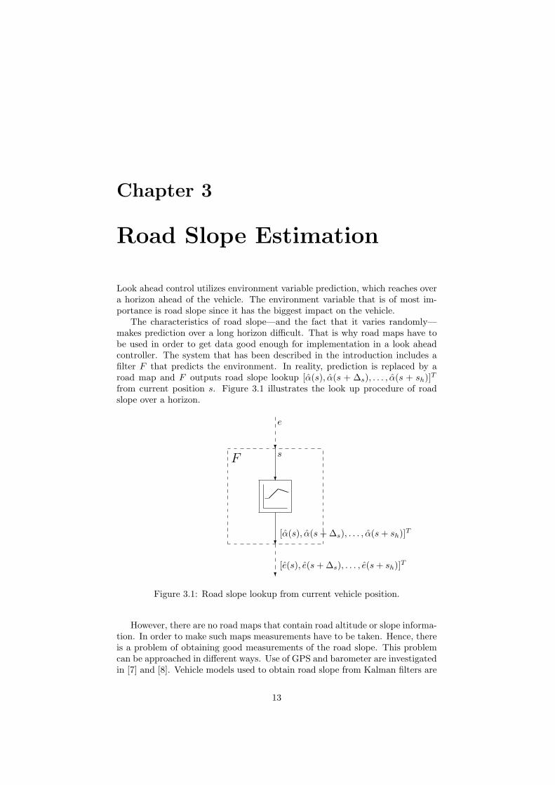
Look ahead control utilizes environment variable prediction, which reaches overa horizon ahead of the vehicle. The environment variable that is of most im-portance is road slope since it has the biggest impact on the vehicle.

The characteristics of road slope—and the fact that it varies randomly—makes prediction over a long horizon difficult. That is why road maps have tobe used in order to get data good enough for implementation in a look aheadcontroller. The system that has been described in the introduction includes afilter F that predicts the environment. In reality, prediction is replaced by aroad map and F outputs road slope lookup [α(s), α(s + Δs), . . . , α(s + sh)]T

from current position s. Figure 3.1 illustrates the look up procedure of roadslope over a horizon.

�

�

�

�

F

e

s

[α(s), α(s + Δs), . . . , α(s + sh)]T

[e(s), e(s + Δs), . . . , e(s + sh)]T

����

Figure 3.1: Road slope lookup from current vehicle position.

However, there are no road maps that contain road altitude or slope informa-tion. In order to make such maps measurements have to be taken. Hence, thereis a problem of obtaining good measurements of the road slope. This problemcan be approached in different ways. Use of GPS and barometer are investigatedin [7] and [8]. Vehicle models used to obtain road slope from Kalman filters are

13

described in [9] and [8]. Laser scanning is another method, presented in [10].This chapter discusses one approach to road slope estimation. The method

used is described and estimation results of a road segment are presented. Prob-able errors when estimating road slope are discussed and will later be used insensitivity analysis in Chapter 5 providing realistic road slope noise.

3.1 Kalman Filter

Assume there is a time discrete system with states x described by

xk = f(xk−1, ωk−1)yk = h(xk, wk),

where xk is equivalent to x(k). Inputs to the system are zero mean whiteprocess noise ω and measurement noise w. The noise sources have time varyingcovariance matrices Qk and Rk.

An observer of the system is given in

xk = f(xk−1, 0) + K(yk − h(xk−1, 0)),

with gain K weighing difference between measurement yk and prediction of themeasurement h(xk−1, 0).

The linear Kalman filter, see [11], assumes that evolution function f andobservation function h are linear in states x and in noise ω and w. Gain K isthen chosen such that it minimizes

E[(xk − xk)2].

However, evolution function f in road slope estimation is non-linear andthe linear Kalman filter cannot be applied. Instead, there is an extension tothe linear Kalman filter that handles non-linearities in the system. This is theextended Kalman filter (EKF) and is described in detail in [8]. EKF stateobservation can be described in two steps.

First a time update is calculated with estimate xk|k−1 and estimate errorcovariance Pk|k−1 as

xk|k−1 = f(xk−1, 0)

Pk|k−1 = FkPkFTk + ΩkQkΩT

k ,

where Fk and Ωk are the partial derivative matrices of f with respect to x andω respectively, defined as

Fk =∂f

∂x(xk−1, 0)

Ωk =∂f

∂ω(xk−1, 0).

The second step in EKF is the measurement update with gain Kk, estimatexk and estimate error covariance Pk according to

Kk = Pk|k−1HTk

(HkPk|k−1H

Tk + WkRkWT

k

)−1

xk = xk|k−1 + Kk

(yk − h(xk|k−1, 0)

)

Pk =(I − KkHk

)Pk|k−1,

14

where Hk and Wk are partial derivative matrices of h with respect to x and w,defined as

Hk =∂h

∂x(xk−1, 0)

Wk =∂h

∂w(xk−1, 0).

3.2 Vehicle and Environment Model

When estimating road slope, a time discrete state space model representingvehicle and environment is used, characterized by

xk = f(xk−1, ωk−1)yk = h(xk, wk). (3.1)

Process noise ω and measurement noise w are assumed zero mean and whitewith diagonal covariance matrices Qk and Rk. State vector x is defined as

x = [ Te Tf α v s z pw pz ]T

and contains eight states representing vehicle and environment.States of the vehicle are engine torque Te, engine friction torque Tf and

velocity v. Environment states represent position s, altitude z, road slope αand the outside pressure, which is divided into two components. pz is the partof the outside pressure which changes with altitude, while pw represents pressurecaused by weather changes.

The states in (3.1) are assumed to evolve in discrete time according to thefollowing equations, where T is sampling time.

Te,k+1 = Te,k + ω1

Tf,k+1 = Tf,k + ω2

αk+1 = αk + ω3

vk+1 = vk + Tc1(c3(Te,k + Tf,k) − c2v2k − c6 sin(αk + c7)) + ω4

sk+1 = sk + Tvk + ω5

zk+1 = zk + Δzk + w6 = zk + Tvk sin(αk) + ω6

pw,k+1 = pw,k + ω7

pz,k+1 = pz,k + μ1Δzk + μ2Δzk(2zk + Δzk) + ω8

Both engine torque and engine friction torque are hard to model and are forthat reason assumed to be white processes. The reason for having both states isthat they have different noise variance, especially when the driving conditionschange e.g. when braking.

Road slope α is assumed to be constant with additive white noise as input.Vehicle velocity state evolution is the same as in the basic vehicle model

except for the brake torque which has been omitted. Brake torque is hard toestimate and for that reason a model that is valid only when not braking hasbeen chosen. Note that the constants c1, . . . , c7 have replaced natural vehicleconstants for easier overview. As vehicle constants should, they change withdifferent gears.

15

Position on road is an integration of the velocity state.Altitude evolution is also an integration where Δzk equals the distance trav-

eled in height last T seconds.Pressure is divided into two parts. Weather caused pressure is assumed to

vary slowly and is modeled as constant with small noise variance. Altitudecaused pressure is affected by the altitude change Δzk, according to a secondorder approximation of the standard altitude pressure function.

Observation vector y in (3.1) is

y = [ Te Tf vGPS vtacho vABS sGPS stacho zGPS p ]T ,

containing engine torque Te, engine friction torque Tf , GPS velocity signal vGPS ,tachometer velocity measurement vtacho, ABS velocity signal vABS , GPS dis-tance signal sGPS , tachometer distance measurement stacho and GPS altitudesignal zGPS .

Observation function h(xk, wk) describes how states xs and measurementvariance wk produce a measurement yk. The relationships are

Te,k =100

TmaxTe,k + w1

Tf,k =100

TmaxTf,k + w2

vGPS,k = 3.6 vk + w3

vtacho,k = 3.6 vk + w4

vABS,k = 3.6 vk + w5

sGPS,k = sk − sGPS(0) + w6

stacho,k = sk − stacho(0) + w7

zGPS,k = zk + w8

pk = pw,k + pz,k + w9.

As can be seen in the equations, engine torque and engine friction torque aremeasured in percent of maximum torque Tmax. All three velocity measurementsare obtained in the unit m/s. Further, distance measurements are corrected withtheir initial value so that the starting point equals position zero. GPS altitudedata is mapped to the altitude state directly, while barometer pressure datacorresponds to the sum of weather and altitude caused pressure.

3.3 Filter Design and Results

Road slope estimation is performed by applying the extended Kalman filter inSection 3.1 to the vehicle and environment system in Section 3.2. The imple-mentation is straight forward, with the exception of choosing noise covariance.As described earlier, covariance matrices Qk and Rk are designed to get desiredfilter behaviour. The design procedure of noise covariance is described below.Also corresponding results are presented. The correctness of the results is hardto establish since the true road slope is not known. Instead, focus is put ongetting the same results even when unexpected events occur.

The first step in designing covariance matrices is to assume that they arediagonal, which simplifies the relation between input noise and output. The

16

covariance matrices are

Qk =

⎛⎜⎜⎜⎝

σ2ω1,k

0 0 00 σ2

ω2,k0 0

0 0 σ2ω3,k

0...

......

. . .

⎞⎟⎟⎟⎠ , Rk =

⎛⎜⎜⎜⎝

σ2w1,k

0 0 00 σ2

w2,k0 0

0 0 σ2w3,k

0...

......

. . .

⎞⎟⎟⎟⎠ ,

where diagonal elements σ2i represent noise variance of each noise source i. Next,

events that occur in the system, e.g. satellite loss, have to be handled. This isdone by making the covariance matrices dependent of such events. Each possibleevent is described below.

3.3.1 Steady Driving

From the system equations in Section 3.2 it is realized that there are threedifferent ways of obtaining road slope estimation. The GPS and the barometerboth provide altitude estimates that can be differentiated in order to obtainroad slope. Also, the velocity evolution equation implicitly gives a value of roadslope. These three sources of information have to be weighed so that the mostaccurate information shows in the estimate.

When driving at a steady pace and all sensors are active, Qk and Rk arechosen so that road altitude and slope vary smoothly. Values of covariancematrices are chosen with variances

σ2ωk

=[5 × 102, 5 × 103, 1 × 10−5, 1, 1, 1 × 10−3, 1 × 10−4, 1 × 10−1

]T

σ2wk

=[1, 1 × 103,

1 × 103

γsats, 1, 1,

1 × 103

γsats, 1,

1 × 103

γsats, 1 × 10−4

]T

,

where γsats denotes number of available satellites. As seen, more satellites giveless measurement variance.

Estimation on Swedish road E20 from Strangnas to Kjula gives the resultsdepicted in Figure 3.2.

17

0 0.5 1 1.5 2 2.5 3

x 104

20

40

60

80

Alti

tude

[m]

0 0.5 1 1.5 2 2.5 3

x 104

−10

0

10

Slo

pe [%

]

0 0.5 1 1.5 2 2.5 3

x 104

20

40

60

80

Vel

ocity

[km

/h]

0 0.5 1 1.5 2 2.5 3

x 104

0

5

10

Sat

ellit

es

Position [m]

Steady est.

Figure 3.2: Road E20, Strangnas - Kjula. Steady driving most part of the roadwith all sensors enabled.

3.3.2 Satellite Availability

At least four satellites are needed for the GPS data to be valid. When thereare less than four satellites available, measurement variance of GPS signals isincreased to a large value. Road slope has to be obtained from other sensorsand covariance values are changed to

σ2ωk

=[5 × 102, 5 × 103, 5 × 10−7, 0, 1, 1 × 10−3, 0, 1 × 10−5

]T

σ2wk

=[1, 1 × 103, 1 × 1012, 1, 1, 1 × 1012, 1, 1 × 1012, 1 × 10−3

]T.

Figure 3.3 depicts simulated GPS data loss in position interval 10 − 20 km.

18

0 0.5 1 1.5 2 2.5 3

x 104

20

30

40

50

60

70

80

90

Alti

tude

[m]

0 0.5 1 1.5 2 2.5 3

x 104

−10

−5

0

5

10

Slo

pe [%

]

Position [m]

Steady est.No GPS est.

Figure 3.3: Road E20, Strangnas - Kjula. No GPS data is used in the interval10 - 20 km, simulating satellite connection loss. Barometer data is relied on toa greater extent giving a more quantized estimation of road altitude.

One can argue that the barometer does not provide much information aboutroad slope since it outputs a quantized signal. Figure 3.4 shows estimationresult when both GPS and barometer data are neglected. It is obvious thatroad altitude and slope are estimated lower than they are when barometer datais used.

19

0 0.5 1 1.5 2 2.5 3

x 104

−20

0

20

40

60

80

Alti

tude

[m]

0 0.5 1 1.5 2 2.5 3

x 104

−10

−5

0

5

10

Slo

pe [%

]

Position [m]

Steady est.No GPS & bar est.

Figure 3.4: Road E20, Strangnas - Kjula. No GPS or barometer data usedin the interval 10 - 20 km. Estimation results illustrate the importance of abarometer in the case when satellite connection is lost. Road altitude and slopeestimates differ from true values significantly.

3.3.3 Shifting Gears and Braking

No torque is delivered to the wheels when shifting gears. This event is handledby simply setting a very high variance on engine torque and engine frictiontorque noise. Also variance of road slope is reduced to assure that it does notchange too much while shifting. When a gear is in place again, process varianceis restored to its initial value and constants c1, . . . , c7 are updated to appropriatevalues.

Braking adds another torque to the velocity evolution equation, and is veryhard to estimate correctly. That is why brake torque has not been modeledand why the equation is not valid when braking. Hence, all braking is handledexactly the same way as when shifting gears.

The covariance values used when shifting gears or braking are

σ2ωk

=[1 × 1015, 1 × 1015, 1 × 10−5, 1, 1, 1 × 10−3, 1 × 10−4, 1 × 10−1

]T

σ2wk

=[1, 1 × 103,

1 × 103

γsats, 1, 1,

1 × 103

γsats, 1,

1 × 103

γsats, 1 × 10−4

]T

.

To obtain realistic gear shifts and braking jerky drive data were recorded onthe same road as previously. Figure 3.5 depicts how the estimation changed.

20

0 0.5 1 1.5 2 2.5 3

x 104

20

40

60

80

Alti

tude

[m]

0 0.5 1 1.5 2 2.5 3

x 104

−10

0

10

Slo

pe [%

]

0 0.5 1 1.5 2 2.5 3

x 104

20

40

60

80

Vel

ocity

[km

/h]

0 0.5 1 1.5 2 2.5 3

x 104

0

5

10

Gea

r nu

mbe

r

Position [m]

Steady est.Jerky est.

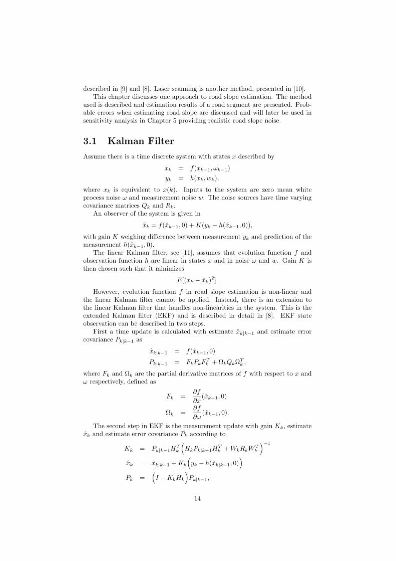
Figure 3.5: Road E20, Strangnas - Kjula. Jerky driving is detected in gearchanges and swift velocity changes. The effects of jerky driving are seen in roadaltitude and slope estimation.

3.4 Conclusions

The road slope estimation filter that has been designed uses data from standardvehicle sensors and GPS. Road altitude and slope have been estimated for aSwedish road segment and results look satisfying. Noise covariances are used asfilter design parameters adjusted so that the filter gives a good estimate evenwhen parts of input data are not available. However, full confidence in thefilter will be gained only when there is a true road profile available and filterperformance can be evaluated more rigorously.

21

Chapter 4

Look Ahead Control

The look ahead control problem is discussed in this chapter. Section 4.1 definesthe optimal look ahead problem in a general way. Solutions to approximateproblems are presented in Sections 4.2 and 4.3. Also, simulations are presentedfor chosen roads that illustrate controller behaviour and fuel consumption sav-ings.

4.1 Optimal Look Ahead

Look ahead control is studied in order to improve the cruise controller. For thatreason one should expect that its performance is at least as good as that of itspredecessor. How to verify this is not straight forward. There is a questionof driver approval of control behaviour, e.g. no jerky control. A more easy todefine requirement is reduced fuel consumption compared to a cruise controller.These two controller properties are discussed below.

Consider the general look ahead system in Figure 1.1. Assume that theenvironment is fully represented by road slope α and that the road slope isknown. Also assume that vehicle parameters m and rw are estimated perfectly.The system changes to that in Figure 4.1 and an optimization problem can beformulated as follows. Find a controller

u = C(v, vref , α,m, rw),

that minimizes the cost function

minu

J = minu

∫ s+sh

s

δ ds, (4.1)

for the following system

[v δ]T = S(u, α)

t =1v, (4.2)

with initial conditions

v(0) = vref

t(0) = t0 (4.3)

22

��

�

� �

��u

δ

v

vref

α

m, rw

C S

�

Figure 4.1: Look ahead controller system assuming that road slope is known.

and constraints

s ∈ [0, sh]v(s) ∈ [vmin, vmax]

v(s + sh) > 0

t(s + sh) =sh

vref− t0. (4.4)

A solution to this optimal control problem results in a velocity profile vthat the vehicle represented by system S should hold in order to minimize fuelconsumption J while respecting the time constraint t(s + sh) and set minimumand maximum velocities, vmin and vmax. However, there are cases when asolution to the problem does not exit, e.g. an uphill slope steep and long enoughthat vmin cannot be respected. Note that system S that represents the vehiclecan be chosen freely.

The optimal look ahead controller will, by solving the optimal problem for arealistic vehicle model S, fulfill the following requirements when there exists asolution. These requirements are such that if a controller fulfills them, the driverhas no reason not to trust it. Hence, they are a must for an implementation.

1. Vehicle speed must not be greater than vmax.

2. Vehicle speed must not be lower than vmin.

3. Vehicle velocity is vref , unless some smart control is implemented to han-dle altitude variations.

4. Driving a distance on a typical road takes an amount of time that iscomparable to that of a cruise controller.

23

5. Fuel consumption is better than that of a cruise controller, at worst com-parable.

4.2 Expert Cruise Control

Expert cruise control (ECC), is a control strategy which relies on logical reason-ing of how a driver should control the vehicle in order to solve the optimizationproblem. It is thoroughly described in [2].

4.2.1 Control Algorithm

Assume that a vehicle

[v(s), δ(s)]T = S(u(s), α(s))

is modeled with the SHTL model in Section 2.2 with control signal

u(s) = [vset(s), δcut(s)]T .

From experience it is known that fuel savings can be made when drivingup or down slopes that are steep and long. For this reason, driving is dividedinto three main states. These are driving on a fairly plain road and driving upand down hills. Distinction between the three states is made with precalculatedvehicle and mass specific values for road slope.

Plain road: When driving on a flat road much cannot be done to save fuel.Hence the vehicle cruise controller SCC is allowed to control the vehicle.

u = (vref , 0)

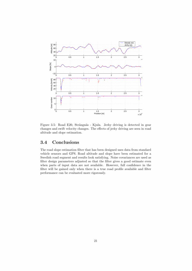
Uphill slope: An uphill slope is defined such that it causes the vehicle to losespeed, even though maximum fueling is applied. This means that if theslope is long enough, velocity drops below vmin. A good driver counteractsthis behaviour by increasing the speed before the slope. ECC applies thesame strategy.

u = (vref , 0)

u = (vmax, 0)

u = (vref , 0)

Figure 4.2: Two distinct positions are calculated when approaching an uphillslope. The control signal changes at these positions.

A position before the slope is calculated, at which ECC starts to acceleratethe vehicle by requesting vmax as set speed for the cruise controller. This

24

position is such that vmax is reached in the beginning of the slope. vmax iskept as set velocity until the slope ends, from where the reference velocityis used again.

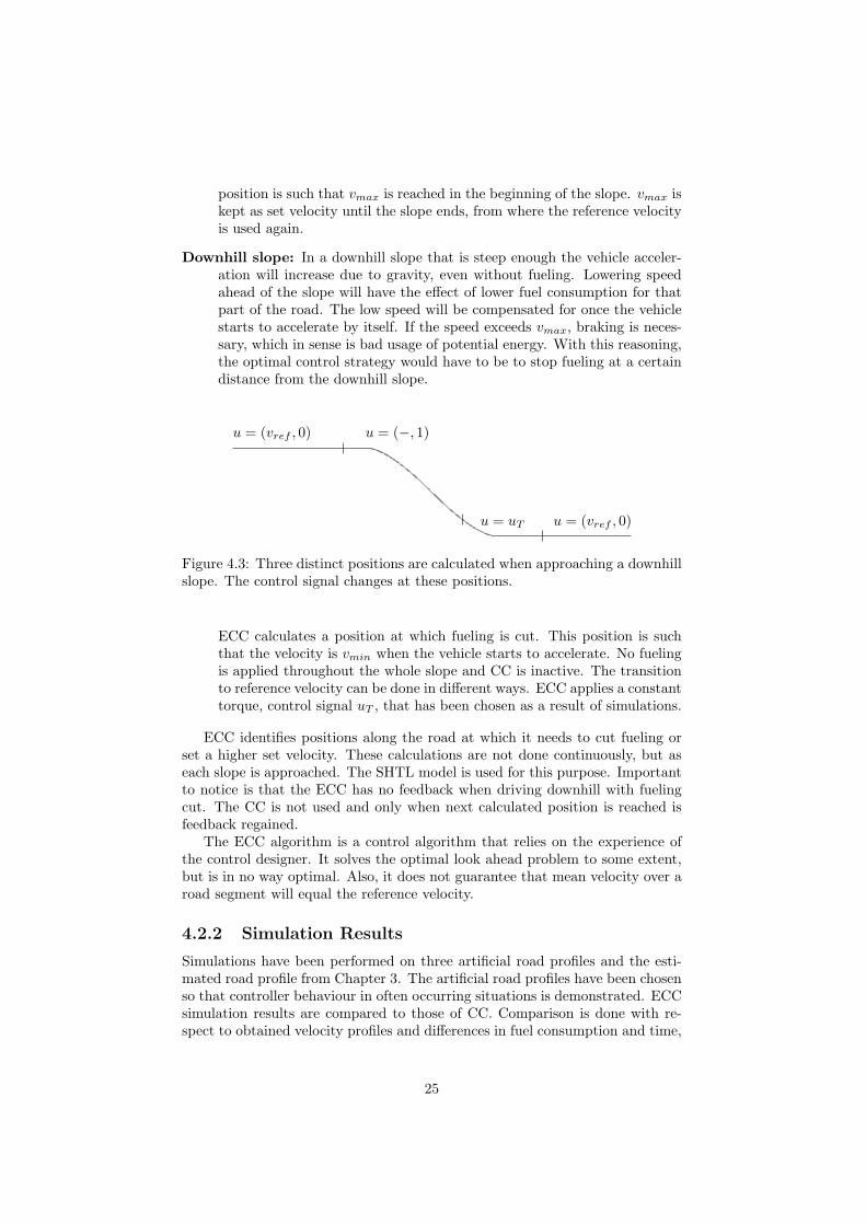
Downhill slope: In a downhill slope that is steep enough the vehicle acceler-ation will increase due to gravity, even without fueling. Lowering speedahead of the slope will have the effect of lower fuel consumption for thatpart of the road. The low speed will be compensated for once the vehiclestarts to accelerate by itself. If the speed exceeds vmax, braking is neces-sary, which in sense is bad usage of potential energy. With this reasoning,the optimal control strategy would have to be to stop fueling at a certaindistance from the downhill slope.

u = (vref , 0) u = (−, 1)

u = uT u = (vref , 0)

Figure 4.3: Three distinct positions are calculated when approaching a downhillslope. The control signal changes at these positions.

ECC calculates a position at which fueling is cut. This position is suchthat the velocity is vmin when the vehicle starts to accelerate. No fuelingis applied throughout the whole slope and CC is inactive. The transitionto reference velocity can be done in different ways. ECC applies a constanttorque, control signal uT , that has been chosen as a result of simulations.

ECC identifies positions along the road at which it needs to cut fueling orset a higher set velocity. These calculations are not done continuously, but aseach slope is approached. The SHTL model is used for this purpose. Importantto notice is that the ECC has no feedback when driving downhill with fuelingcut. The CC is not used and only when next calculated position is reached isfeedback regained.

The ECC algorithm is a control algorithm that relies on the experience ofthe control designer. It solves the optimal look ahead problem to some extent,but is in no way optimal. Also, it does not guarantee that mean velocity over aroad segment will equal the reference velocity.

4.2.2 Simulation Results

Simulations have been performed on three artificial road profiles and the esti-mated road profile from Chapter 3. The artificial road profiles have been chosenso that controller behaviour in often occurring situations is demonstrated. ECCsimulation results are compared to those of CC. Comparison is done with re-spect to obtained velocity profiles and differences in fuel consumption and time,

25

defined as

Δfuel =fuelECC − fuelCC

fuelCC

Δtime =timeECC − timeCC

timeCC.

A plain road is characterized by zero road slope. The controller of a vehicleshould at all times hold set reference velocity, even look ahead controllers.

When driving on a plain road the ECC will use the CC, meaning that thevehicle will hold the reference speed. An illustration of such a simulation isomitted because of its simplicity.

A 500 m uphill slope of 3 % is simulated with results in Figure 4.4. Asdescribed earlier, the ECC accelerates the vehicle at a distinct position givingthe desired behaviour. More fuel than with CC is actually used, but the meanvelocity is higher and overall closer to the reference.

0 500 1000 1500 2000 25000

5

10

15

Alti

tude

[m]

Δfuel: 0.67 %Δtime: −1.15 %

0 500 1000 1500 2000 2500

80

85

90

Vel

ocity

[km

/h]

−− vref

0 500 1000 1500 2000 25000

50

100

150

200

250

Fue

ling

[mg/

stro

ke]

Position [m]

ECCCC

ECCCC

Figure 4.4: Simulation of ECC algorithm on road with a 500 m 3 % uphill slopeand a 40 ton SHTL model vehicle.

Simulations on a road with a 500 m 3 % downhill slope give the resultsdepicted in Figure 4.5. A position where fueling is cut is calculated and no fuelis injected until the end of the slope. A transition period of 300 meters is seenand then the vehicle cruise controller retains control. 12.21 % of fuel is savedover a distance of 3 km with a negligible difference in time.

A simulation of a drive on the estimated road segment from Strangnas toKjula gives the results depicted in Figure 4.6. It can be seen that the ECCidentifies five slope segments where a strategy different from CC is applied.Fuel savings are 1.43 %.

26

0 500 1000 1500 2000 2500−15

−10

−5

0A

ltitu

de [m

]

Δfuel: −12.21 %Δtime: 0.91 %

0 500 1000 1500 2000 2500

80

85

90

Vel

ocity

[km

/h]

−− vref

0 500 1000 1500 2000 25000

50

100

150

Fue

ling

[mg/

stro

ke]

Position [m]

ECCCC

ECCCC

Figure 4.5: Simulation of ECC algorithm on road with a 500 m 3 % downhillslope and a 40 ton SHTL model vehicle.

0 0.5 1 1.5 2 2.5

x 104

0

20

40

Alti

tude

[m]

Δfuel = −1.43 %Δtime = 0.07 %

0 0.5 1 1.5 2 2.5

x 104

−5

0

5

Slo

pe [%

]

0 0.5 1 1.5 2 2.5

x 104

80

85

90

Vel

ocity

[km

/h]

0 0.5 1 1.5 2 2.5

x 104

0

100

200

Fue

ling

[mg/

stro

ke]

Position [m]

ECCCC

ECCCC

Figure 4.6: Road E20, Strangnas - Kjula. Simulation of ECC algorithm with a40 ton SHTL vehicle.

27

4.3 Model Predictive Cruise Control

Model predictive control (MPC) is a control strategy that solves optimal controlproblems. A controller based on MPC has been implemented in [3] in an attemptto solve the optimal look ahead problem. The control algorithm and simulationresults are described below.

4.3.1 Control Algorithm

Assume that a vehicle

[v(s), δ(s)]T = S(u(s), α(s))

is modeled with the basic model in Section 2.3 with control signal

u(s) = [P (s), G(s), B(s)]T .

A cost function J is defined as

J(s) =

s+shΔs∑

k=s

Q1δk + Q2κ(ek)e2k + Q3|vk − vk+1| + Q4κ(|Gk − Gk+1|) + Q5Bk

where ek = vk − vref,k and κ is a step function

κ(x) ={

1 x > 00 x ≤ 0

and xk = x(k).For each position step s of Δs meters, the MPC algorithm

1. Finds the optimal control signal u∗(s), u∗(s+Δs), ..., u∗(s+ sh) that min-imizes the cost function J(s). Optimization is handled with dynamicprogramming and is described in detail in [3]. Important to know is thatit includes many simulations of vehicle model S.

2. Implements the control signal u∗(s) for Δs meters.

3. Starts from 1 when position s + Δs is reached.

Since prediction of output of vehicle model S has to be done for a big numberof possible control signals, the model has to be simplified. A great deal of timecan be saved if engine and fueling maps can be approximated by functions. Anapproximation S of the vehicle model is obtained with function approximationsof Tmap and δmap and is used in the MPC algorithm.

[v(s), δ(s)]T = S(u(s), α(s))

The strategy of MPC is to use the control signal that minimizes a cost func-tion depending on all possible future control signals and corresponding predictedsystem outputs. An optimization problem is in fact solved each Δs meters.However, this optimization problem is different from the general optimizationproblem defined in Section 4.1 in several points. There are no constraints onfinal velocity and time states, as in (4.4), meaning that mean velocity doesnot necessarily have to equal the reference velocity. Also, the cost function isdifferent giving the controller a behaviour that is not always desired.

28

4.3.2 Simulation Results

Simulation results of the MPC algorithm are performed on the same roads asfor the ECC. Comparison of MPC results is done with those of a PI controllerimplemented on the basic vehicle model. Comparison is as earlier done withrespect to obtained velocity profiles and differences in fuel consumption andtime, this time defined as

Δfuel =fuelMPC − fuelPI

fuelPI

Δtime =timeMPC − timePI

timePI.

Simulation results with the MPC algorithm on a plain road are shown inFigure 4.7. Clearly the MPC algorithm does not manage to keep the referencevelocity of 85 km/h. This is a result of the approximation of engine and fuelingmaps. A somewhat higher mean velocity is held and the control is not constant.This results in higher fuel consumption (0.70 %) and faster travel time (0.19%).

0 200 400 600 800 1000 1200 1400 1600 1800−1

−0.5

0

0.5

1

Alti

tude

[m]

Δfuel = 0.70 %Δtime = −0.19 %

0 200 400 600 800 1000 1200 1400 1600 180084

84.5

85

85.5

86

Vel

ocity

[km

/h]

−− vref

0 200 400 600 800 1000 1200 1400 1600 18000

50

100

Ped

al le

vel [

%]

Position [m]

MPCPI

MPCPI

Figure 4.7: Simulation of MPC algorithm on plain road with a 40 ton basicmodel vehicle.

29

Simulations on a road with a 500 m uphill slope of 3 % have been carriedout. Results are shown in Figure 4.8. The MPC algorithm increases the fuelingamount ahead of the slope in order to get a greater velocity when reaching it.This behaviour resembles the one of an experienced driver and is expected fromlook ahead controllers. The fueling amount is held at a high level throughoutthe slope. The controller does not manage to restore vehicle velocity to thereference one kilometer after the slope, but stabilizes at a lower velocity.

0 500 1000 1500 2000 25000

5

10

15

Alti

tude

[m]

Δfuel = −0.39 %Δtime = −0.69 %

0 500 1000 1500 2000 2500

80

85

90

Vel

ocity

[km

/h]

−− vref

0 500 1000 1500 2000 25000

50

100

Ped

al le

vel [

%]

Position [m]

MPCPI

MPCPI

Figure 4.8: Simulation of MPC algorithm on road with a 500 m 3 % uphill slopeand a 40 ton basic model vehicle.

30

Simulations with a 500 m downhill slope of 3 % have been performed. Theresults are presented in Figure 4.9. A decrease in velocity is noted ahead ofthe downhill slope. The MPC algorithm behaves correctly, reacting on theapproaching slope. Fuel savings compared to a PI controller are 8.61 %.

0 500 1000 1500 2000 2500−15

−10

−5

0

Alti

tude

[m]

Δfuel = −8.61 %Δtime = 0.52 %

0 500 1000 1500 2000 250080

85

90

Vel

ocity

[km

/h]

−− vref

0 500 1000 1500 2000 25000

50

100

Ped

al le

vel [

%]

Position [m]

MPCPI

MPCPI

Figure 4.9: Simulation of MPC algorithm on road with a 500 m 3 % downhillslope and a 40 ton basic model vehicle.

31

The MPC algorithm has been simulated on the same estimated road segmentas ECC. Results are shown in Figure 4.10 and it is clear that controller behaviourseen in previous simulations is present even here. However, the MPC algorithmdoes not manage to save any fuel for this particular road segment, but uses 2.10% more than a PI controller. The reasons for this have not been investigatedsince they fall out of the scope of this thesis.

0 0.5 1 1.5 2 2.5

x 104

0

20

40

Alti

tude

[m]

Δfuel = 2.10 %Δtime = −0.04 %

0 0.5 1 1.5 2 2.5

x 104

−5

0

5

Slo

pe [%

]

0 0.5 1 1.5 2 2.5

x 104

75

80

85

90

Vel

ocity

[km

/h]

−− vref

0 0.5 1 1.5 2 2.5

x 104

0

50

100

Ped

al le

vel [

%]

Position [m]

MPCPI

MPCPI

Figure 4.10: Road E20, Strangnas - Kjula. Simulation of MPC algorithm witha 40 ton basic model vehicle.

4.4 Conclusions

Two different strategies implemented in order to solve a problem that resemblesthe optimal look ahead problem have been described. Both have demonstratedfuel savings when simulations on isolated slopes have been performed in theirrespective simulation environments. However, when simulations on an estimatedroad slope are performed the MPC algorithm fails to reduce fuel consumption.It is important to notice that fuel savings figures cannot be compared betweenthe two environments since they use different vehicle models.

Even though the strategies differ it is clear that obtained velocity profilesin the two implementations are alike. This gives a confidence in the presentedsolution. A disadvantage that the MPC algorithm has is that it fails in keepinga reference velocity on a plain road and takes long to recover after uphill slopes.The ECC on the other hand sometimes totally lacks feedback, which shows inthe sensitivity analysis presented in the following chapter.

32

Chapter 5

Sensitivity Analysis

Performance of the presented controllers in perfect conditions has been thor-oughly described in [2] and [3]. Good controller behaviour and fuel savingshave been demonstrated. The sensitivity analysis in this chapter is a naturalstep before actual implementation of a look ahead controller that is based oneither strategy.

Sources of disturbances in a look ahead implementation are identified andrealistic values of their magnitude are given in Section 5.1. Effects on controllerbehaviour caused by disturbances are presented and discussed in Section 5.2.Finally, conclusions are drawn in Section 5.3 in the light of the results.

5.1 Sources of Disturbances

Reality is not perfect and there is no such thing as perfect conditions. The aimof the sensitivity analysis is to identify realistic disturbances which have a bigimpact on the system and how the impact shows. Several disturbances will bea factor in an implementation. These can be divided into two types, differencesbetween vehicle model and vehicle and errors in available road slope data. Thesetwo types are discussed in this chapter and procedures of testing their impacton the results are described.

Figure 5.1 provides an illustration of the system with possible error sources.It is good to refer to in order to get a more intuitive understanding.

33

��

�

� �

��

�� �α

α

���

m, rw m, rw

uδ

v

vref

α

m, rw

C S

�

Figure 5.1: Look ahead controller system overview with error sources.

5.1.1 Model Inflicted Errors

Differences between the model that a controller uses and the real system causemodel inflicted erroneous behaviour. Look ahead controllers described in Chap-ter 4 assume that vehicle mass and wheel radius are known parameters. How-ever, in reality they cannot be estimated precisely and are for this reason obvioussources for errors.

Several papers discuss mass estimation, e.g. [9], and the general understand-ing is that mass is hard to estimate if road slope is not known, and vice versa.This is a result of the fact that it is hard to distinguish mass from slope inestimation. A look at the gravity force equation reveals the reason.

Fg = mg sin α = (m + m)g sin α = (1 + Δ)mg sin α

As seen, a relative error Δ in mass might as well be a relative error in sin α,which for small slopes approximates to α. Thus, an error in mass might as wellbe considered as an error in road slope. Mass estimation can be off by as muchas ten percent. ∣∣∣∣mm

∣∣∣∣ ≤ 10%

Another error that is highly probable, is error in wheel radius. A truck tyrehas an approximate wheel radius of 50 cm. An error of two percent, or onecentimeter, is analyzed. ∣∣∣∣ rw

rw

∣∣∣∣ ≤ 2%

34

5.1.2 Road Slope Inflicted Errors

Look ahead controllers have the advantage of having information about theroad slope ahead. If that information is not correct it inflicts errors. There areseveral reasons why this information could be wrong. When performing analysisa model for the error is needed. Assuming the error is additive,

α = α + α,

α can be modeled in several ways.The most obvious model for α is white Gaussian noise with different vari-

ances. Motivation for this model is simply that it excites all frequencies in thesystem. Its impact will be tested on a plain road, a constant uphill slope and aconstant downhill slope for different noise variances.

α ∈ N(0, σ2α)

σα = 0.005 rad

Lags and errors in GPS data can result in wrong position parameters, whichreflects in road slope. If the controller gets an input on position saying that thevehicle is 50 meters further down the road, control will be implemented with alag of 50 meters. These types of errors can be seen as a delay in road slope data,either positive or negative. Simulations will be done on a plain road, a constantuphill slope and a constant downhill slope with delays up to 50 meters.

α(s) = α(s + Δs)Δs ∈ {−50,−25, 0, 25, 50}

Braking and jerky driving is known to cause bad estimation of road slope. Inparticular, there is sometimes a question of whether velocity decrease is causedby braking or an uphill slope. For this reason, the impact of bad estimation dueto jerky driving will be simulated, using the estimated road slope in Chapter 3.

5.2 Simulation Results

Simulations with disturbances stated above have been performed. Main differ-ences from behaviour of the controllers in perfect conditions are presented belowwith corresponding plots.

5.2.1 Expert Cruise Control

Expert cruise control is made up in two steps. The first is identification ofslopes where some other strategy than maintaining the reference velocity willbe used. The other is calculation of positions along the road where anothercontrol signal will be applied. Simulations with disturbances mentioned aboveaffect both steps in the controller.

If the road slope at a certain point along the road has such a value that itlies close to the limit deciding whether a slope will be treated or not, a smallerror in road slope will have a big effect on the controller. This is illustrated inFigure 5.2 where two simulations are compared. A simulation of a drive on aroad estimated with data from a steady drive is compared to a drive on the same

35

road with the exception that the controller has access to road slope estimatedfrom data of a jerky drive. It is obvious that different strategies are chosen atseveral points along the road, as an effect of different road slope estimation. Forexample, the jerky drive slope estimate around position 15 km is higher thanthe steady drive estimate, why the ECC decides to keep a higher velocity whenapproaching the slope.

0 0.5 1 1.5 2 2.5

x 104

0

20

40

Alti

tude

[m]

ECC

0 0.5 1 1.5 2 2.5

x 104

−5

0

5

Slo

pe [%

]

0 0.5 1 1.5 2 2.5

x 104

80

85

90

Vel

ocity

[km

/h]

0 0.5 1 1.5 2 2.5

x 104

0

100

200

Fue

ling

[mg/

stro

ke]

Position [m]

Steady est.Jerky est.

Figure 5.2: Road E20, Strangnas - Kjula. Comparison between simulations ofECC when road slope is estimated from a steady drive and a jerky drive. Smalldifferences in road slope lead to big differences in control strategy.

36

When a slope where strategy change will be implemented has been located,simulations with the SHTL model are performed in order to decide where toswitch control. Incorrect data on vehicle mass and/or road slope will make thesesimulations inaccurate giving points that are not where they should be. Theeffect is most visible in a simulation plot of a drive on a downhill slope. Figure 5.3illustrates how the strategy switch points are moved when the position valueis 50 meters off in either direction. Two effects that are not acceptable can beseen. If the controller changes control signal too early the limit on minimumvelocity is not respected, since no feedback is present in this controller state. Ifthe control signal is changed too late the velocity of the vehicle will be lowerwhen returning to the reference and a jerky behaviour is obtained, characterizedby an impulse in fueling.

0 500 1000 1500 2000 2500−15

−10

−5

0

Alti

tude

[m]

ECC

0 500 1000 1500 2000 2500

80

85

90

Vel

ocity

[km

/h]

0 500 1000 1500 2000 25000

100

200

Fue

ling

[mg/

stro

ke]

Position [m]

Δs = 0mΔs = 50mΔs=−50m

Δs = 0mΔs = 50mΔs=−50m

Figure 5.3: Comparison of three simulations of ECC algorithm on road with a500 m 3 % downhill slope and a 40 ton SHTL model vehicle. Road slopes inthe simulations are shifted in position by 50 meters in each direction, causingunwanted controller behaviour.

37

5.2.2 Model Predictive Cruise Control

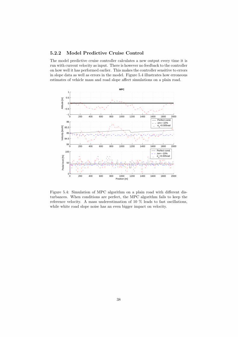
The model predictive cruise controller calculates a new output every time it isrun with current velocity as input. There is however no feedback to the controlleron how well it has performed earlier. This makes the controller sensitive to errorsin slope data as well as errors in the model. Figure 5.4 illustrates how erroneousestimates of vehicle mass and road slope affect simulations on a plain road.

0 200 400 600 800 1000 1200 1400 1600 1800 2000−1

−0.5

0

0.5

1

Alti

tude

[m]

MPC

0 200 400 600 800 1000 1200 1400 1600 1800 200084

84.5

85

85.5

86

Vel

ocity

[km

/h]

0 200 400 600 800 1000 1200 1400 1600 1800 20000

50

100

Ped

al le

vel [

%]

Position [m]

Perfect cond.Δm=−10%σα=0.005rad

Perfect cond.Δm=−10%σα=0.005rad

Figure 5.4: Simulation of MPC algorithm on a plain road with different dis-turbances. When conditions are perfect, the MPC algorithm fails to keep thereference velocity. A mass underestimation of 10 % leads to fast oscillations,while white road slope noise has an even bigger impact on velocity.

38

No feedback in form of earlier performance also leads to the possibility ofstabilizing at another solution than what is intended. Figure 5.5 shows how anerror in mass or position can lead to a stable solution with a velocity other thanthe reference when the road ahead is plain.

0 500 1000 1500 2000 25000

5

10

15

Alti

tude

[m]

MPC

0 500 1000 1500 2000 2500

80

85

90

Vel

ocity

[km

/h]

0 500 1000 1500 2000 25000

50

100

Ped

al le

vel [

%]

Position [m]

Perfect cond.Δm=−10%Δs=50m

Perfect cond.Δm=−10%Δs=50m

Figure 5.5: The MPC algorithm has problems returning to reference velocityafter an uphill slope. When an underestimation in mass of 10 % or a miscal-culation in position of 50 meters is present, the velocity settles 2 km/h belowreference.

39

As with the ECC, the MPC makes distinctions between different slopes andapplies different strategies. However, the MPC does not commit to a decisionbut has the ability to alter the control signal every new iteration. The effect ofthis is that strategy changes due to erroneous road slope estimation are moreseldom as can be seen in Figure 5.6.

0 0.5 1 1.5 2 2.5

x 104

0

20

40

Alti

tude

[m]

MPC

0 0.5 1 1.5 2 2.5

x 104

−5

0

5

Slo

pe [%

]

0 0.5 1 1.5 2 2.5

x 104

75

80

85

90

Vel

ocity

[km

/h]

−− vref

0 0.5 1 1.5 2 2.5

x 104

0

50

100

Ped

al le

vel [

%]

Position [m]

Steady est.Jerky est.

Figure 5.6: Road E20, Strangnas - Kjula. Comparison between simulations ofMPC when road slope is estimated from a steady drive and a jerky drive. Smalldifferences in road slope lead to difficulties in following the reference as well asdifferences in strategy.

40

5.3 Conclusions

The results from the sensitivity analysis show that both investigated controllersare in a pre development state and that a lot of work needs to be done in orderto make them worthy of an implementation. Besides this enlightenment, thesensitivity analysis has resulted in a number of interesting conclusions aboutthe strategies that the controllers implement.

Feedback is important in all control systems. It is also important to beaware of what type of feedback that is necessary. The ECC has no feedback oncertain road segments and this leads to violation of problem constraints. TheMPC gets feedback all the time. However, it is not used to correct the previouscontrol signal, why unwanted settling points can occur.

Errors in estimated vehicle mass and road slope affect control performance.Expected vehicle behaviour is not true and control that is not suited for theroad is implemented. This is shown in clear strategy changes for both ECC andMPC.

41

Chapter 6

Conclusions

This thesis has looked into two implementation aspects of look ahead cruisecontrollers. These are road slope information and control sensitivity.

Road slope estimation is an important part of look ahead since there cur-rently are no road maps containing such information. A road slope estimationfilter using standard heavy vehicle sensors and GPS data has been designed.Importance has been attached to designing a robust filter that can deal withlosses in input data as well as events giving an invalid model. Satisfying resultshave been obtained. The filter has also been used as a realistic noise source, dif-ferences in estimations have been considered as probable road slope estimationerrors.

Sensitivity analysis of look ahead cruise controllers is an important stepbefore an implementation. Two controllers that use different control strategieshave been tested with errors in estimated vehicle parameters and road slope.The differences in control strategy give control errors that are direct results ofchosen approaches.

Designing a controller based on experience has proven to work well, althoughtwo main design aspects have shown to be sensitive. Lack of feedback whendriving down a hill gives velocities that do not respect given bounds and evenjerky fuel injection. Small differences in slope that lie around certain limit valuesgive distinct differences in control. Such vehicle behaviour is not desirable sincedrivers might experience it as indecisive.

Look ahead cruise control based on model prediction has advantages as wellas disadvantages. Constant feedback giving updated control signals is a featurethat is essential for several reasons. Primarily, interaction with other systemsthat might have inputs like time dependent reference or maximum velocities. Adrawback with the considered version is that feedback is not used in order tocorrect previous control signals as much as it could, making the controller verysensitive to vehicle model and road slope errors. Consequences caused by thisare oscillating velocity and stabilization on speeds other than the reference.

42

Chapter 7

Future Work andExtensions

The developed filter has been tuned so that the road estimation is preservedwhen partial data is not available. A tuning with respect to a true road profilewould give confidence in the presented solution. The Swedish Road Adminis-tration is performing measurements on a number of selected roads in Sweden.This data could provide a base for tuning and a more rigorous validation of thefilter.

The investigated controllers clearly need to be improved before an implemen-tation is carried out. One topic that is important is the interface between thecontroller and the vehicle. Using a simple cruise controller that is controlled bya look ahead algorithm is preferable out of several reasons. Most importantly,it gives a clear limit between different levels of control in the system.

Integration of Look Ahead Cruise Control with Adaptive Cruise Controlis the next step in vehicle cruise control. Using the knowledge of presence ofvehicles ahead and their velocity is a source of information that needs to beincluded in the calculation in order to get a cruise controller that behaves asgood as any skilled driver.

43

Bibliography

[1] Lattemann. F et al. (2004). The Predictive Cruise Control - A System toReduce Fuel Consumption of Heavy Duty Trucks. SAE Paper, 2004-01-2616.

[2] Wingren, A. (2005). Fordonsreglering med framforhallning. M.Sc. Thesis.Linkoping, Linkoping University.

[3] Hellstrom, E. (2005). Explicit use of road topography for model predictivecruise control in heavy trucks. M.Sc. Thesis. Linkoping, Linkoping Univer-sity.

[4] Kiencke, U. & Nielsen, L. (2005). Automotive Control Systems - For En-gine, Driveline, and Vehicle. Berlin: Springer-Verlag.

[5] Bengtsson, P. (2004). Simulation of Models Intended for Complete VehicleSimulation. M.Sc. Thesis. Uppsala, Uppsala University.

[6] Sandberg, T. (2001). Heavy Truck Modeling for Fuel Consumption Simu-lations and Measurements. Lic. Thesis. Linkoping, Linkoping University.

[7] Seo, J., Lee, J. G. & Park, C. G. (2004). Bias Suppression of GPS Mea-surement in Inertial Navigation System Vertical Channel. Position Locationand Navigation Symposium, pp. 143-147.

[8] Johansson, K. (2005). Road Slope Estimation with Standard Truck Sensors.M.Sc. Thesis. Stockholm, Royal Institute of Technology.

[9] Lingman, P. & Schmidtbauer, B. (2002). Road Slope and Vehicle MassEstimation Using Kalman Filtering. Vehicle System Dynamics Supplement,37, pp. 12-23.

[10] Ahlin, K., Granlund J. & Lindstrom F. (2004). Comparing Road Profileswith Vehicle Perceived Roughness. International Journal of Vehicle Design.Vol. 36, No. 2/3.

[11] Hjalmarsson H. & Ottersten B. (2002). Lecture Notes in Adaptive SignalProcessing. Course material. Stockholm, Royal Insitute of Technology.

44