los alamos space weather summer school research reports€¦ · 2015 los alamos space weather...

2015 Los Alamos Space Weather Summer School

Research Reports

Misa M. Cowee (Editor)

Cover image: SOHO EIT image (sohowww.nascom.nasa.gov)


Research Reports

Misa M. Cowee (Editor)


Research Reports

i

Preface

The fifth Los Alamos Space Weather Summer School was held June 1st – July 24th, 2015, at Los Alamos National Laboratory (LANL). With renewed support from the Institute of Geophysics, Planetary Physics, and Signatures (IGPPS) and additional support from the National Aeronautics and Space Administration (NASA) and the Department of Energy (DOE) Office of Science, we hosted a new class of five students from various U.S. and foreign research institutions. The summer school curriculum includes a series of structured lectures as well as mentored research and practicum opportunities. Lecture topics including general and specialized topics in the field of space weather were given by a number of researchers affiliated with LANL.

Students were given the opportunity to engage in research projects through a mentored practicum experience. Each student works with one or more LANL-affiliated mentors to execute a collaborative research project, typically linked with a larger on-going research effort at LANL and/or the student’s PhD thesis research. This model provides a valuable learning experience for the student while developing the opportunity for future collaboration.

This report includes a summary of the research efforts fostered and facilitated by the Space Weather Summer School. These reports should be viewed as work-in-progress as the short session typically only offers sufficient time for preliminary results. At the close of the summer school session, students present a summary of their research efforts.

It has been a pleasure for me to be the director of the Los Alamos Space Weather Summer School this year. I am very proud of the work done by the students, mentors and lecturers—your dedicated effort and professionalism are key to a successful program. I am grateful for all the administrative and logistical help I have received in organizing the program. Los Alamos, NM Dr. Misa Cowee November 2015 Summer School Director


Research Reports

ii

New students Yuxi Chen University of Michigan Ravindra Desai University College London, UK Ehab Hassan University of Texas at Austin Nadine Kalmoni University College London, UK Dong Lin Virginia Polytechnic Institute and State University

Returning students Sebastian De Pascuale University of Iowa R. Scott Hughes University of Southern California Hong Zhao University of Colorado Boulder


Research Reports

iii

Project Reports New Students Full Particle-in-Cell (PIC) Simulation of Whistler Wave Generation Mentors: Gian Luca Delzanno and Yiqun Yu Student: Yuxi Chen …………….……………………………………………………………….. 1 Hybrid simulations of the right-hand ion cyclotron anisotropy instability in a sub-Alfvénic plasma flow Mentor: Misa Cowee Student: Ravindra Desai ………...……………………………………………………….......... 9 A Statistical Ensemble for Solar Wind Measurements Mentors: Steven Morley and John Steinberg Student: Ehab Hassan ……………………...………………………………………………….. 17 Observations and Models of Substorm Injection Dispersion Patterns Mentor: Michael Henderson Student: Nadine Kalmoni ……………………...…………………………………………….... 32 Heavy Ion Effects on Kelvin-Helmholtz Instability: Hybrid Study Mentors: Misa Cowee and Xiangrong Fu Student: Dong Lin ……………………...………………………………………………………. 44 Returning Students Simulating Plasmaspheric Electron Densities with a Two-Component Electric Field Model Mentor: Vania Jordanova Student: Sebastian De Pascuale…………………………………………………………….... 52


Research Reports

iv

Ion and Electron Heating by Whistler Turbulence: Parametric Studies via Particle-In-Cell Simulation Mentor: S. Peter Gary and Misa Cowee Student: R. Scott Hughes………………………………………………………………….….... 64 The statistics of relativistic electron pitch angle distribution in the Earth’s radiation belt based on the Van Allen Probes measurements Mentor: Reiner Friedel Student: Hong Zhao ..…………………………………………………………..........................73


Research Reports

v

Pictures

Class of 2015 Students and Mentors (Students indicated in bold. Left to right, back row: John Steinberg, Reiner Friedel, Steve Morley, Mike Henderson, Xiangrong Fu; middle row: Sebastian DePascaule, Ehab Hassan, Hong Zhao, Dong Lin, Yuxi Chen, R. Scott Hughes; front row: Ravi Desai, Josefina Salazar, Misa Cowee, Nadine Kalmoni, Vania Jordanova. Not pictured: Gian Luca Delzanno, Yiqun Yu, and Peter Gary.


Research Reports

vi

Lectures

• Python Tutorial ............................................................................ Steve Morley • Introduction to the Solar Wind ................................................... Joe Borovsky • Introduction to Detectors for High Energy Particles, X-rays, and Gamma rays

....................................................................................................... Richard Schirato • A Magnetospheric Overview ........................................................ Geoff Reeves • Adiabatic particle motion, Drift shells, and Radiation belt ....... Mike Henderson • Geomagnetic Storms, Ring Current, and Plasmasphere ........... Vania Jordanova • Magnetosphere-Ionosphere Coupling .......................................... Yiqun Yu • Space Plasma Instrument Design ............................................... Brian Larsen • Introduction to Plasma Waves ..................................................... Peter Gary • Kinetic Plasma Instabilities ......................................................... Peter Gary • Statistics for Space Science ......................................................... Steve Morley • PIC Simulation Technique ........................................................... Xiangrong Fu • Magnetic Reconnection ................................................................ Bill Daughton • Energetic Particles in the Solar System .................................... Fan Guo • Hazards to Satellites from the Space Environment ................... Heather Quinn • Data Assimilation ........................................................................ Humberto Godinez • Electromagnetic Waves ................................................................ Max Light


Research Reports

vii

Sponsors

• Institute of Geophysics, Planetary Physics, and Signatures (IGPPS) • National Aeronautics and Space Administration (NASA) • Department of Energy - Office of Science (DOE-OSC)

Contact Information Dr. Misa Cowee Los Alamos Space Weather Summer School P.O. Box 1663, MS D466 Los Alamos National Lab, NM 87545 http://www.swx-school.lanl.gov/

Publication Release LA-UR 15-29127

Full Particle-in-Cell(PIC) Simulation of Whistler Wave Generation

Yuxi Chen

Center for Space Environment Modeling, University of Michigan, Ann Arbor, Michigan, USA

Yiqun Yu

Beihang University, Beijing, China

Gian Luca Delzanno

Los Alamos National Laboratory, New Mexico, USA

Abstract

Whistler waves are considered as an important mechanism for both electrons acceleration and precipitation in the

radiation belts. The generation and propagation of whistler waves have drawn great attention in the space physics

field. As a preliminary study to understand the development of electron temperature anisotropy, the generation and

propagation of whistler waves, and the influence of inhomogeneous magnetic field, we performed a series of one-

dimensional and two-dimensional simulations using the implicit particle-in-cell (iPIC3D) code. Both initial conditions

and boundary conditions are explored. A one-dimensional system with a uniform background magnetic field and

either a uniform or localized plasma distribution is studied. For the localized plasma distribution the wave packets

propagation is affected by the presence of the edge density gradient. A two-dimensional self-consistent simulation

with curved magnetic field and localized plasma distribution is performed and analyzed. After the development of

the whistler instability and the propagation of transmitted and reflected wave packets, at a later time the frequency

spectrum shifts to higher frequencies due to wave-wave interaction of wave-packets that are artificially reflected from

the boundary of the system.

Keywords: particle-in-cell, whistler wave

1. Introduction

Whistler mode waves are electromagnetic emissions frequently observed in the inner magnetosphere. The fre-

quency of whistler waves is between ion gyro-frequency and electron gyro-frequency. The whistler waves with narrow

band of frequency-time spectrum are called chorus waves, which are often observed outside the plasmapause in the

dawn sector ((Meredith et al., 2001)).

Chorus waves are important for both electrons acceleration and precipitation in radiation belt. It has been observed

that chorus waves can accelerate electrons to relativistic speed in the outer radiation belt (Horne and Thorne, 1998;

Horne et al., 2005; Thorne et al., 2013). Chorus wave can also scatter energetic particles into loss cone, and cause

the electrons’ precipitation to the ionosphere, which is an important source of aurora (Thorne et al., 2010). It has

been generally accepted that the chorus waves are generated by the temperature anisotropy of electrons (Omura et al.,

2008), which may be introduced by the injections of plasma sheet electrons from the tail of magnetosphere (Horne

and Thorne, 2003; Jordanova et al., 2010).

Several numerical models have been developed to study the generation and evolution of chorus waves. The

Vlasov-hybrid simulation has been used to generate both rising-tone and falling-tone successfully (Nunn, 1990; Nunn

Email addresses: [email protected] (Yuxi Chen), [email protected] (Yiqun Yu), [email protected] (Gian Luca

Delzanno)

2015 Los Alamos Space Weather Summer School Research Reports 1

and Omura, 2012). Katoh and Omura (2007) used a 1D electron hybrid code, in which the background cold electrons

are described as a fluid while the energetic electrons are treated as particles, to generate rising-tone chorus. This

one-dimensional code assumes an azimuthal symmetric parabolic field to represent the spatial inhomogeneity of

Earth’s dipole field. Using the same field configuration, Hikishima et al. (2009) performed a full particle-in-cell

(PIC) simulation, and Tao (2014) used a hybrid code, DAWN, studied the wave intensity variation of chorus waves.

However, all these models are one-dimensional, and they are not fully self-consistent when dealing with a spatially

varying magnetic field. To get more self-consistent results, Wu et al. (2015) used a two-dimensional hybrid code to

study the generation and propagation of chorus waves on a generalized coordinate system.

During the geomagnetic active times, the energetic particles injected from the tail to the ring current may be-

come anisotropic because of the inhomogeneity of the background magnetic field. These electrons with temperature

anisotropy can generate chorus waves due to the whistler anisotropy instability (Gary and Wang, 1996). The waves

are generated and propagates on the dipole field, and the non-uniform background field leads to the rising-tone chorus

waves (Katoh and Omura, 2007). Our final goal is to understand the development of the electron anisotropy, the role

of inhomogeneous magnetic field, the generation and propagation of whistler wave. As a preliminary study, we use

the implicit particle-in-cell (iPIC3D) code (Markidis et al., 2010) to learn about the generation and propagation of the

chorus wave on both uniform and spatially varying background magnetic field.

In the next section, the iPIC3D code is briefly introduced. Section 3 describes the simulation setup, and discusses

the simulation results. Finally the conclusion is presented in section 4.

2. The implicit particle-in-cell (iPIC3D) code

∇ · E = 4πρ (1)

∇ · B = 0 (2)

∂B∂t= −c∇ × E (3)

∂E∂t= c∇ × B − 4π J (4)

dpdt= q(E +

V × Bc

) (5)

The particle-in-cell (PIC) method has been extensively used in the plasma physics field. It directly solves the

Maxwell’s equations (eq. (1) to eq. (4)) to update electromagnetic field, and moves particles via Newton’s equa-

tion (eq. (5)). The basic idea of PIC is not difficult. Super-particles1 are moving around on the grid following the

Newton’s equation, and the fields are updated based on the charge density and current, which are determined by super-

particles. The disadvantage of PIC is that it is very time consuming because most computational time is used to move

super-particles and many super-particles are needed to suppress the statistical noise. Explicit methods are widely used

to solve these time-evolution equations. However, the explicit particle-in-cell method is suffering from the stability

constraints (Lapenta, 2012):

• The Courant - Friedrichs - Lewy (CFL) condition: Δt < Δxc .

• Time step should be small enough to resolve the highest frequency motion, which is plasma frequency here:

Δt < 2ωpe

.

• Finite grid instability: Δx < c0λDe, c0 ∼ π.These constrains limit both spatial resolution (Δx) and time step (Δt), so it is very difficult for explicit particle-in-

cell code to simulate large scale system. To break down these constrains, we need to solve the time-evolution equations

1A super particle is a computational particle that represents many real particles

Y. Chen, PIC Simulation of Whistler Wave Generation


in a implicit manner. Markidis et al. (2010) developed the iPIC3D code, it transforms the Maxwell’s equations into a

second order derivative form:

∂2 E∂t2= c2∇2 E − 4π

∂ J∂t− 4πc2∇ρ (6)

and update the electric field with an implicit solver. Particles are also moved implicitly. So, the iPIC3D code is

unconditionally stable and not limited by the constrains we discussed above, and large grid size and time step can be

used, which is important for large scale simulations. In practice, the iPIC3D code still needs to satisfy the accuracy

constraint: Δt < Δx/vth, where vth is the thermal velocity of particles, in order to get accurate results. Since the time

step is not limited by the stability constrains, it can be larger than particle gyro-period. To ensure the gyro-motion is

resolved, the sub-cycling technique is used (Peng et al., 2015) in iPIC3D.

3. Simulation setup and Results

We want to simulate how the chorus waves develop when anisotropic energetic electrons are injected into the

ring current. But it is not trivial to get the background equilibrium distribution as initial condition nor to set proper

boundary conditions. Non-equilibrium initial condition may drive instabilities, and the boundary conditions are also

crucial for PIC simulations (Naitou et al., 1979). As a preliminary study, we focus on the injected anisotropic electrons

and ignore the background cold electrons. Since the injected electrons are concentrated on the Earth’s equator, we only

initialize the anisotropic particles in a small region near the center of the simulation domain. These simplifications

avoid the difficulty of setting initial equilibrium initial condition for background plasma. We also use some simple

boundary conditions, like periodic boundary or Neumann boundary. We will explore the role of boundary conditions

in the future.

3.1. 1D simulation with uniform backgroundWe started from a 1D simulation with uniform background density and magnetic field. Because it is easy to

setup and can give us some basic knowledge about both numerical parameters and physics of whistler waves. The

simulation is initialized with uniform background magnetic field B = (0, 0, 150)nT on a domain with LZ = 500c/ωpe.

The electrons are initialized with uniform density ne = 6cm−3, and anisotropy temperature T‖ = 1kev and T⊥ = 4kev.

Cold ions with the same number density are used to keep charge neutrality. Based on our numerical experiments, we

choose Δz = 0.05c/ωpe, Δt = 0.13ω−1pe and 1000 super-particles in each cell. Periodic boundary conditions are used

for both fields and particles.

The simulation results at t = 248/Ωce2 is shown in Figure 1. The whistler waves generate the fields perpendicular

to the propagation direction, and the non-zero parallel electric filed Ez is caused by statistic noise. We can see that the

disturbed perpendicular fields form several wave packets. The wave observed at the middle point of the simulation

domain is shown in Figure 2. We can see the chorus wave develops from uniform background and forms several wave

packets. The frequency of the waves are about 0.4Ωce or 0.45Ωce (bottom of Figure 2), which is the frequency of

a typically chorus wave. Further analysis shows that different frequencies corresponding to different wave-packets.

We also analyze the dominant wave mode in the simulation domain, and found it shifts from large wavenumber

(kdominant ∼ 1.2ωpe/c at t = 50Ω−1ce ) to small wavenumber (kdominant ∼ 0.8ωpe/c at t = 125Ω−1

ce ), which is consistent

with previous studies (Lu et al., 2010).

3.2. 1D simulation with localized plasma distributionUsing the same background magnetic field and numerical parameters, we only distribute particles uniformly in

the middle (200 < z < 300) of the domain. Since electrons have larger thermal velocity than ions, we may expect the

charge separation at the edges of the plasma distribution.

The results at t = 248/Ωce are shown in Figure 3. As we expected, the charge separation appears and builds

localized electric field in z direction, which is the same order as the noise. Figure 4 shows the By wave in a time-space

plane. The waves grow and propagate toward both sides. When the wave reach the shape density gradient locations,

part of the wave is transmitted and part of the wave is reflected. The reflected wave may interact with other waves.

2Time is normalized by ωpe in the code, but we show the results in terms of Ωce in this report.



Figure 1: The generation of whister wave on 1D grid with uniform background magnetic field. Results at t = 248Ω−1ce are shown. The unit of length

is c/ωpe. Note that all the values are in normilized units.

0 50 100 150 200 250 300 350

tΩce

−0.20

−0.15

−0.10

−0.05

0.00

0.05

0.10

0.15

0.20

By/B0

0.0 0.2 0.4 0.6 0.8 1.0

ωΩce

0

5

10

15

20

25

30

35

Power

Figure 2: Top: the wave observed at the middle of the simulation domain. Bottom: The frequency spectrum.



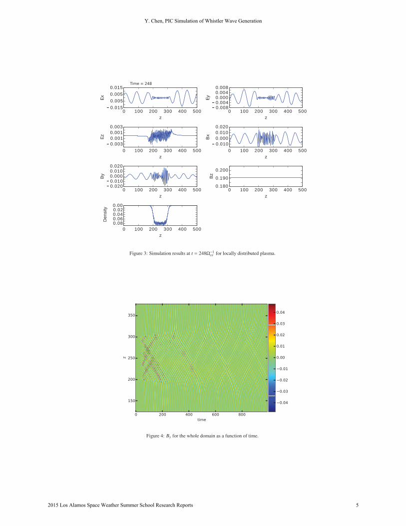
Figure 3: Simulation results at t = 248Ω−1ce for locally distributed plasma.

0 200 400 600 800

time

150

200

250

300

350

z

−0.04

−0.03

−0.02

−0.01

0.00

0.01

0.02

0.03

0.04

Figure 4: By for the whole domain as a function of time.



Figure 5: The initial condition for the 2D simulation with curved magnetic field.

3.3. 2D curved magnetic field

A 2D simulation with curved background magnetic field, which mimics the dipole field of Earth, is conducted.

The simulation domain is (x, z) ∈ [0, 4]× [0, 500]. The initial condition is shown in Figure 5, and the background field

is

Bx = 2c0x(250 − z)B0

By = 0

Bz = (1 + c0(z − 250)2)B0

where B0 = 250nT and c0 = 1.6 × 10−5c−2Ω2ce. The background field is similar to the one used by Katoh and Omura

(2007), except that By is always zero here. The plasma is only uniformly distributed between z = 200 and z = 300.

Since the background magnetic field does not change too much for (x, z) ∈ [0, 4] × [200, 300], this initial distribution

will not cause significant instability during the simulation. In z direction, Neumann boundary is applied for disturbed

fields and open boundary is used for particles. Other simulation parameters are the same as these 1D simulations.

The wave observed at x = 2c/ωpe and z = 260c/ωpe is shown in Figure 6, where we can also see the formation of

chorus wave packets. Interestingly, the frequency shifts from about 0.6Ωce at t ∼ 80Ω−1ce to 1.3Ωce at t ∼ 220Ω−1

ce . This

turns out to be related to the boundaries and caused by the wave-wave interaction, which can be seen from Figure 7.

Figure 7 shows By along z direction as a function of time. Similar to the 1D case, waves can be reflected when density

gradient becomes large. At t ∼ 220Ω−1ce and z ∼ 260c/ωpe. The reflected waves create the wave observed at z ∼ 260

with very high frequency.



0 50 100 150 200 250 300 350 400

tΩce

−0.06

−0.04

−0.02

0.00

0.02

0.04

0.06

By/B0

0.0 0.2 0.4 0.6 0.8 1.0 1.2 1.4

ωΩce

0.00

0.01

0.02

0.03

0.04

0.05

0.06

0.07

0.08

Power

Figure 6: Top: By ovserved at x = 0 and z = 260. Bottom: the spectral power of By.

0 50 100 150 200 250 300 350

time

0

100

200

300

400

500

z

−0.020

−0.015

−0.010

−0.005

0.000

0.005

0.010

0.015

0.020

Figure 7: The wave By in the 2D simulation along z direciton as a function of time.



4. Conclusion

As the first step to study the development of anisotropy, the role of inhomogeneous magnetic field, and the genera-

tion and propagation of whistler waves, we conducted a series of one-dimensional and two-dimensional particle-in-cell

simulations that start from a bi-Maxwellian plasma with a predefined level of temperature anisotropy. The whistler

instability then develops and chorus wave packets are observed.

We explored the influence of the initial and boundary conditions of the system. In particular, we have studied a

one-dimensional system with a uniform background magnetic field and either a uniform or localized plasma distri-

bution. The early behavior of the system is similar in both cases, but for the localized plasma distribution the wave

packets propagation is affected by the presence of the edge density gradient and transmitted and reflected wave packets

develop. A two-dimensional self-consistent simulation with inhomogeneous background magnetic field and localized

plasma distribution is performed, showing the importance of the boundary conditions in the system. After the de-

velopment of the whistler instability and the propagation of transmitted and reflected wave packets, at a later time

the frequency spectrum shifts to higher frequencies due to wave-wave interaction of wave-packets that are artificially

reflected from the boundary of the system.

Future work will focus on characterizing the transmitted/reflected wave packets and the role of the inhomogeneous

magnetic field.

References

Gary, S.P., Wang, J., 1996. Whistler instability: Electron anisotropy upper bound. Journal of Geophysical Research: Space Physics (1978–2012)

101, 10749–10754.

Hikishima, M., Yagitani, S., Omura, Y., Nagano, I., 2009. Full particle simulation of whistler-mode rising chorus emissions in the magnetosphere.

Journal of Geophysical Research: Space Physics (1978–2012) 114.

Horne, R., Thorne, R., 2003. Relativistic electron acceleration and precipitation during resonant interactions with whistler-mode chorus. Geophys-

ical research letters 30.

Horne, R.B., Thorne, R.M., 1998. Potential waves for relativistic electron scattering and stochastic acceleration during magnetic storms. Geophys-

ical Research Letters 25, 3011–3014.

Horne, R.B., Thorne, R.M., Shprits, Y.Y., Meredith, N.P., Glauert, S.A., Smith, A.J., Kanekal, S.G., Baker, D.N., Engebretson, M.J., Posch, J.L.,

et al., 2005. Wave acceleration of electrons in the van allen radiation belts. Nature 437, 227–230.

Jordanova, V., Thorne, R., Li, W., Miyoshi, Y., 2010. Excitation of whistler mode chorus from global ring current simulations. Journal of

Geophysical Research: Space Physics (1978–2012) 115.

Katoh, Y., Omura, Y., 2007. Computer simulation of chorus wave generation in the earth’s inner magnetosphere. Geophysical research letters 34.

Lapenta, G., 2012. Particle simulations of space weather. Journal of Computational Physics 231, 795–821.

Lu, Q., Zhou, L., Wang, S., 2010. Particle-in-cell simulations of whistler waves excited by an electron κ distribution in space plasma. Journal of

Geophysical Research: Space Physics (1978–2012) 115.

Markidis, S., Lapenta, G., Rizwan-Uddin, 2010. Multi-scale simulations of plasma with ipic3d. Mathematics and Computers in Simulation 80,

1509–1519.

Meredith, N.P., Horne, R.B., Anderson, R.R., 2001. Substorm dependence of chorus amplitudes- implications for the acceleration of electrons to

relativistic energies. Journal of geophysical research 106.

Naitou, H., Tokuda, S., Kamimura, T., 1979. On boundary conditions for a simulation plasma in a magnetic field. Journal of Computational Physics

33, 86–101.

Nunn, D., 1990. The numerical simulation of vlf nonlinear wave-particle interactions in collision-free plasmas using the vlasov hybrid simulation

technique. Computer Physics Communications 60, 1–25.

Nunn, D., Omura, Y., 2012. A computational and theoretical analysis of falling frequency vlf emissions. Journal of Geophysical Research: Space

Physics (1978–2012) 117.

Omura, Y., Katoh, Y., Summers, D., 2008. Theory and simulation of the generation of whistler-mode chorus. Journal of Geophysical Research:

Space Physics (1978–2012) 113.

Peng, I.B., Markidis, S., Vaivads, A., Vencels, J., Amaya, J., Divin, A., Laure, E., Lapenta, G., 2015. The formation of a magnetosphere with

implicit particle-in-cell simulations. Procedia Computer Science 51, 1178–1187.

Tao, X., 2014. A numerical study of chorus generation and the related variation of wave intensity using the dawn code. Journal of Geophysical

Research: Space Physics 119, 3362–3372.

Thorne, R., Li, W., Ni, B., Ma, Q., Bortnik, J., Chen, L., Baker, D., Spence, H.E., Reeves, G., Henderson, M., et al., 2013. Rapid local acceleration

of relativistic radiation-belt electrons by magnetospheric chorus. Nature 504, 411–414.

Thorne, R.M., Ni, B., Tao, X., Horne, R.B., Meredith, N.P., 2010. Scattering by chorus waves as the dominant cause of diffuse auroral precipitation.

Nature 467, 943–946.

Wu, S., Denton, R., Liu, K., Hudson, M., 2015. One-and two-dimensional hybrid simulations of whistler mode waves in a dipole field. Journal of

Geophysical Research: Space Physics 120, 1908–1923.



Hybrid simulations of the right-hand ion cyclotron anisotropy instability in a

sub-Alfvénic plasma flow

Ravindra T. Desai

Mullard Space Science Laboratory, University College London, Holmbury St Mary, RH5 6NT, UK

Misa M. Cowee

Los Alamos National Laboratory, Los Alamos, New Mexico, 87545, USA

Abstract

This report outlines a study of the right-hand ion cyclotron anisotropy instability driven by negatively charged ions in

a sub-Alfvénic plasma flow. A set of hybrid Particle-In-Cell simulations are performed on a multi-ion plasma

consisting of anisotropic ring and maxwellian distributions of positive and negative ions. It was found that the right-

hand instability acts in an analogous manner to the left-hand instability with comparable growth and saturation rates

as predicted by linear dispersion theory. Comparable fluctuations in the electromagnetic fields were also observed

indicating equivalent wave-particle interactions. A number of complexities arose when both instabilities were

generated within the same system. The resultant waves displayed a combination of left and right-hand polarisations

and gyrophase bunching was identified as introducing electrostatic effects which resulted in significant and periodic

magnetic field oscillations and wave amplitudes > 50% greater than expected. Simulated scaling of the wave energy

with ring densities and anisotropies was consequently shown to provide a potential method for diagnosing plasma

conditions in environments containing both positive and negative ions.

Keywords: Sub-Alfvénic flow, Ion Cyclotron Wave, Wave Polarisation

1. Introduction

The electromagnetic ion cyclotron anisotropy instability is driven by a 𝑇⊥ > 𝑇∥ anisotropy in the distribution

function of an ion species. Anisotropic ion populations can be created by the ionisation of neutral atoms where the

newly formed ions are accelerated orthogonally to ambient electric and magnetic fields. The ions are thus energised

and, for a sufficiently high plasma beta, generate a number of electromagnetic instabilities (Gary et al, 1987). The left-

hand ion cyclotron instability has been studied extensively for the cases of single and multi, light and heavy-ion

plasmas (Gary et al, 1989; Cowee et al, 2012; Omidi et al, 2010), and has been observed in-situ in a number of space

environments (Huddleston et al. 1997; Leisner et al. 2006). This paper reports a study on the properties of the left and

right-hand ion cyclotron instabilities in a multi-ion sub-Alfvénic plasma flow consisting of anisotropic distributions

of both positive and negative ions.

In the Solar Wind the ion cyclotron instability is a ubiquitous feature (Jian et al. 2010; Volwerk et al. 2013). Solar

wind ions can possess large supra-Alfvénic velocity components parallel to the interplanetary magnetic field which

results in a Doppler shift between the plasma frame and the observing spacecraft. This frequency shift can cause the

waves to be observed as right-handed polarised although they are left-hand polarised in the plasma frame.

In the Earth’s magnetosphere, anisotropic ring current ions are unstable to the generation of ion cyclotron waves

(Horne and Thorne, 1993). The anisotropies involved in this process however are significantly lower than when the


instability is generated by the ionisation of neutrals. These waves are at the outset left-hand polarised but can undergo

polarisation reversals if they pass through the crossover frequency of the multi-ion plasma in which they are generated

(Hu and Denton 2009). As they propagate outwards from the equatorial regions right-hand polarised waves can thus

be observed.

In Jupiter’s and Saturn’s magnetospheres, ion cyclotron waves are generated by the ionisation of neutral material

(Huddleston et al. 1997; Leisner et al. 2006). The predominantly dipolar magnetic field configurations and corotational

electric fields result in a ‘perpendicular’ sub-Alfvénic pickup geometry. The anisotropic ions form rings in velocity

space unstable to the generation of left-handed ion cyclotron waves which act to scatter and diffuse the ion pitch angle

distributions, restoring thermal equilibrium.

In the vicinity of the Jovian moon Europa, Galileo wave observations displayed bursty characteristics at the

gyrofrequency of a number of species including O2, 𝑆𝑂2, K, 𝑁a and Cl, (Volwerk et al, 2001). At the gyrofrequency

of chlorine the wave ellipticity alternated between negative and positive values, the waves displaying both left and

right-hand polarisations. The absence of polarisation reversals at the gyrofrequency of other elements led to this

phenomena being attributed to the presence of both positive and negative chlorine ion populations. This inference is

supported by the high electron affinity and stable configuration of the chlorine anion, 𝐶𝑙−, the additional electron

filling the atoms outer d-shell. Negatively charged halogens, including chlorine, are also known to be abundant in the

Earth’s D region (Kopp and Fritzenwallner, 1997).

This paper outlines a study investigating the behaviour of the ion cyclotron anisotropy instability driven by heavy

positive and negative ion rings in the Europan plasma environment. Using a hybrid simulation code and drawing

comparisons to linear dispersion theory we answer the following questions: Do anisotropic negative ion distributions

generate the right-hand ion cyclotron instability? Does this instability have fundamentally differently properties to the

left-hand cyclotron instability other than the wave polarisation? Is there any interaction between the left and right-

hand instabilities when they are generated in the same system? Following this we examine whether it is possible to

estimate ion densities at Europa from the wave amplitudes observed by the Galileo spacecraft, using simulated scaling

of the wave energy with ring densities and anisotropies.

2. Methodology

Linear dispersion theory is able to predict the frequencies and growth rates of the ion cyclotron anisotropy

instability but is unable to predict wave-particle interactions (Huddlestone et al, 1998). To capture these effects

Particle-In-Cell (PIC) simulations are employed, a simulation technique which has extensively been applied to the

study of positive ion rings generating left-handed ion cyclotron waves (Cowee et al, 2006, 2009, 2010, 2012). The

hypothesis in this investigation is that negative ion rings will conversely generate right-handed waves, as was the

inference in Volwerk et al, 2001.

The hybrid code developed by Winske & Omidi, 1993, is used in this analysis and has been successfully

shown to reproduce the ion cyclotron anisotropy instability in a number of plasma environments (Gary et al, 1989;

Omidi et al, 2010; Cowee et al, 2012). Ions are specified kinetically with electrons approximated as a massless

neutralising fluid, an approach suited to capturing phenomena at the ion spatial and temporal scales. In this study the

particle positions are resolved along one spatial dimension aligned with the magnetic field, 𝐵0, and the electromagnetic

fields are resolved in three dimensions. This approach is justified as linear dispersion theory predicts main wave power

at parallel propagation (Gary and Madland, 1988). Simulating three dimensions would capture more modes but it has

been shown that in one dimension the physical relation between relative changes in wave amplitudes and growth rates

will remain unchanged with respect to varying background plasma conditions (Cowee et al, 2006).

In the PIC simulations, particles properties are collectively approximated by between 107 − 108

superparticles upon 512 grid cells specified across ~40 proton inertial length scales, 𝑐/𝜔, and timesteps specified as

a function of the ion cyclotron frequency, Ω𝑗 , where 𝑗 denotes the ion species. These interpolated ion properties are

subsequently used as inputs to Darwin’s approximation of the field equations.

R. Desai, Hybrid simulations of the right-hand ion cyclotron anisotropy instability in a sub-Alfvénic plasma flow


In this analysis the plasma considered consists of multiple ion species, either in a zero drift maxwellian

distribution or a ring distribution with 𝑇⊥ > 𝑇∥. Each species has mass, 𝑚𝑗 , and charge state, 𝑍𝑗, normalised to the

proton scale with perpendicular and parallel velocities defined as 𝑉∥𝑗 = (2𝑘𝐵𝑇∥𝑗/𝑚𝑗)1/2, and 𝑉⊥𝑗 = (2𝑘𝐵𝑇⊥𝑗/𝑚𝑗)1/2.

The temperature anisotropy, 𝐴𝑗 = 𝑇⊥𝑗/𝑇∥𝑗, is specified according to the corotational plasma velocity of the Jovian

magnetodisk at ~10𝑅𝐽. Further plasma parameters specified are the plasma beta, 𝛽𝑗 = 2𝜇0𝑛0𝑇∥𝑗/𝐵02,, and the Alfven

velocity, 𝑉𝑎 = 𝐵0/√𝜇0𝑛𝑜𝑚𝑗.

Table 1 and 2 shows the simulation and plasma parameters defined to be characteristic of the sub-Alfvénic

Europan plasma interaction as observed by Galileo. The background plasma species, densities and bulk velocities are

based upon values taken from Paterson, 1999, Kivelson et al, 2009, and Bagenal et al, 2015, and are not expected to

play a significant role in the generation of the ion cyclotron instabilities. Three different simulations are carried out in

this study to examine the growth of this instability under varying conditions. In run I a positive maxwellian chlorine

core and anisotropic chlorine ring are initialised to examine the growth of the left-handed instability in an isotropic

background plasma. In run II a negative chlorine core and ring are initialised to examine the growth of the right-

handed instability. In run III a combination of these two are then simulated to explore the effects associated with these

two instabilities growing side by side within the same system.

3. Results

Figures 1-5 show the simulation results corresponding to the three different simulation cases outlined in table 1.

Figure 1 shows the full 𝜔-𝑘 spectrum normalised to the gyrofrequency of the heavy ion species. In each case the

wave power is concentrated at the heavy ion’s gyrofrequency demonstrating growth of the ion cyclotron instability as

predicted by linear dispersion theory. At this frequency range the right-hand magnetosonic mode is also apparent

although the main wave power is concentrated at the cyclotron wave branch. Run I and run II show similar behaviour,

thus demonstrating that an anisotropic negative ion distribution will generate the ion cyclotron instability in a

comparable manner to an anisotropic positive ion distribution. Run III displays stronger wave power which is expected

as there is twice as much free energy within the system.

Figure 2 tracks the temperature evolution of the various species. In each run the chlorine ring ions scatter, their

energy reducing in the perpendicular direction and increasing in the parallel direction. The chlorine core species acts

to damp the growth of the instability and are consequently heated in the perpendicular direction by a factor of ~4. The

background core population is not expected to undergo any heating unless it has a gyroperiod which allows it to

resonantly interact with the ring species (Huddlestone et al, 1998). In run I this effect is evident in that the similarly

charged background species has a mass/charge ratio of a third of the ring species and is consequently heated by a few

percent. In run II the oppositely charged ring species does not interact with this background population, the only

temperature change of the background species being due to interaction with noise level waves. It is noticeable in run

III that the temperature of the background and chlorine core species oscillate strongly. This effect is not predicted by

linear dispersion analysis or reported in previous hybrid simulations of the ion cyclotron instability in planetary

environments (Cowee et al. 2006, 2009, 2010).

Figure 3 displays the energy-history of the instability as it grows from the noise level and reaches saturation at

time equal to ~50Ω𝑡. Run I and run II have similar growth rates, the slight interaction of the positive chlorine ring

with the background species not appearing to significantly dampen the growth of the instability. Run III shows a

growth rate greater than in run I and run II which is in-line with expectations that an increased ring density should

produce stronger wave growth (Huddlestone et al. 1998). The expectation of run III is then that the growth of the wave

amplitudes will cease at the combined values of runs I and II. Strong oscillations however are observed throughout

run III which significantly increase once the instability has saturated. These oscillations result in energies being

reached which are significantly larger than expected, in this instance an increase of > 50%. These oscillations appear

at twice the chlorine cyclotron frequency and are consequently identified as the half-length electrostatic mode

identified in Omidi et al, 2010, and Bortnik et al, 2010.



Figure 4 shows the helical components of the waveform along the simulation axis stacked in time as the

simulations progresses. The magnetic field oscillations are decomposed into their positive and negative helical

components to display the rotation of the wave with respect to the wave vector, 𝑘. The striations in these plots represent

transverse waves which can be seen to increase in magnitude as they move both parallel and anti-parallel to the

magnetic field. In run I the waves move towards -𝑥 for the positive helical components and towards +𝑥 for the negative

components, thus displaying left-handed wave polarisations. In run II this motion is reversed, indicating right-handed

wave polarisations. Run III shows striations leaning towards both +𝑥 and –𝑥 which can be seen to intersect one another.

This can be taken as evidence that both left-handed and right-handed waves are growing within the system, generated

by the positive and negative ion rings respectively. The precise resultant ellipticity however cannot be determined

from this analysis and the resultant wave’s characteristics therefore require further analysis to determine whether the

left and right-handed components combine to form a linearly polarised wave form or whether both left and right-hand

polarised waves are periodically present.

Figure 5 displays the phase-space of run III at four times within the simulation run. Gyrophase bunching is

evident in this figure with particles being trapped in the parallel direction. This introduces electrostatic effects at twice

the anisotropic ion’s gyrofrequency as ions possessing opposing helical components intersect one another’s path twice

within each gyro-orbit. In Omidi et al, 2010, a half-length electrostatic mode was attributed to oppositely directed

helical components being produced by waves propagating both parallel and anti-parallel to the magnetic field. This

effect appears to be particularly enhanced in a system containing both positive and negative ions with the two

instabilities, the left and right-hand ion cyclotron anisotropy instability, growing simultaneously and producing both

right and left handed wave propagating in both directions along the field lines.

Figure 6 represents a further study where the ion densities and anisotropies were varied in order to constrain the

parameter space within which the ion cyclotron waves were generated at Europa. The growth and saturation of the

right-hand ion cyclotron anisotropy instability was found to scale similarly to the left-hand instability with respect to

varying ion densities, pickup velocities and anisotropies. This study can be seen to provide a method for diagnosing

local plasma conditions from observed wave amplitudes, although further analysis is required to understand the

complexities involved in a system containing both positive and negative ions.

4. Conclusions

1D hybrid simulations of positive and negative anisotropic ion distributions were shown to reproduce the left and

right-hand cyclotron instability and to reproduce wave-particle interactions which linear dispersion theory does not

account for. Spectral analysis of the resultant waves showed left and right-handed ion cyclotron waves were indeed

generated by positive and negatively charged anisotropic ion populations. The growing waves were shown to be

analogous to one another the difference being the wave polarisation. Significant complexities resulted in simulations

which contained both positive and negative ions with the multitude of waves generated not displaying a clear resultant

polarisation.

Significant effects were also observed in the interaction between the left and right-handed ion cyclotron

anisotropy instabilities. An electrostatic half-length mode was identified as acting at twice the cyclotron frequency

which resulted in significantly larger magnetic field amplitudes than anticipated. A scaling study on the effects of

varying ion densities and anisotropies was also performed to understand how these changes affected the resultant wave

amplitudes once the instability had saturated. This parametric study demonstrated how it was possible to use this

simulation technique to constrain the local plasma conditions at Europa, although further analysis is required to

understand the electrostatic effects and spectral properties associated with the generation of both the left and right-

handed waves within the same system.

References

Bagenal, F, E S, R J. Wilson, T A. Cassidy, V Dols, F. J. Crary, A J. Steffl, P A. Delamere, W S. Kurth, and W R. Paterson. 2015. “Plasma

Conditions at Europa’s Orbit.” Icarus 261: 1–13. doi:10.1016/j.icarus.2015.07.036.



Bortnik, J., R. M. Thorne, and N. Omidi. 2010. “Nonlinear Evolution of EMIC Waves in a Uniform Magnetic Field: 2. Test-Particle Scattering.”

Journal of Geophysical Research 115 (A12): A12242. doi:10.1029/2010JA015603.

Cowee, M M, S P Gary, and H Y Wei. 2012. “Pickup Ions and Ion Cyclotron Wave Amplitudes Upstream of Mars: First Results from the 1D

Hybrid Simulation.” Geophysical Research Letters 39 (8): L08104–L08104. doi:10.1029/2012GL051313.

Cowee, M M, R J Strangeway, C T Russell, and D Winske. 2006. “One-Dimensional Hybrid Simulations of Planetary Ion Pickup : Techniques

and Verification.” Journal of Geophysical Research 111: 1–9. doi:10.1029/2006JA011996.

Cowee, M. M., and S. P. Gary. 2012. “Electromagnetic Ion Cyclotron Wave Generation by Planetary Pickup Ions: One-Dimensional Hybrid

Simulations at Sub-Alfvénic Pickup Velocities.” Journal of Geophysical Research 117 (A6): A06215. doi:10.1029/2012JA017568.

Cowee, M. M., S. P. Gary, H. Y. Wei, R. L. Tokar, and C. T. Russell. 2010. “An Explanation for the Lack of Ion Cyclotron Wave Generation by

Pickup Ions at Titan: 1-D Hybrid Simulation Results.” Journal of Geophysical Research: Space Physics 115 (July): 1–12. doi:10.1029/2010JA015769.

Cowee, M. M., N. Omidi, C. T. Russell, X. Blanco-Cano, and R. L. Tokar. 2009. “Determining Ion Production Rates near Saturn’s Extended Neutral Cloud from Ion Cyclotron Wave Amplitudes.” Journal of Geophysical Research: Space Physics 114: 1–10.

doi:10.1029/2008JA013664.

Gary, S. P., and C. D. Madland. 1988. “Electromagnetic Ion Instabilities in a Cometary Environment.” Journal of Geophysical Research 93: 235–

41.

Gary, S. Peter, Kazuhiro Akimoto, and Dan Winske. 1989. “Computer Simulations of Cometary-Ion/ion Instabilities and Wave Growth.” Journal

of Geophysical Research 94 (A4): 3513. doi:10.1029/JA094iA04p03513.

Gary, S. P. Shriver, D. 1987. “The Electromagnetic Ion Cyclotron Beam Anisotropy Instability.” Planetary and Space Science 35 (1): 51–59.

Horne, Richard B., and Richard M. Thorne. 1993. “On the Preferred Source Location for the Convective Amplification of Ion Cyclotron Waves.” Journal of Geophysical Research 98: 9233–47. doi:10.1029/92JA02972.

Hu, Y., and R. E. Denton. 2009. “Two-Dimensional Hybrid Code Simulation of Electromagnetic Ion Cyclotron Waves in a Dipole Magnetic Field.” Journal of Geophysical Research 114 (A12): A12217. doi:10.1029/2009JA014570.

Huddleston, D. E., R. J. Strangeway, J. Warnecke, C. T. Russell, M. G. Kivelson, and F. Bagenal. 1997. “Ion Cyclotron Waves in the Io Torus during the Galileo Encounter: Warm Plasma Dispersion Analysis.” Geophysical Research Letters 24 (17): 2143–46.

doi:10.1029/97GL01203.

Huddlestone, D E, R. J. Strangeway, J Wamecke, C T Russell, and M G Kivelson. 1998. “Ion Cyclotron Wave in the Io Torus: Wave Dispersion

Analysis and SO2+ Source Rate Estimates.” Journal of Geophysical Research 103: 887–99.

Jian, L. K., C. T. Russell, J. G. Luhmann, B. J. Anderson, S. a. Boardsen, R. J. Strangeway, M. M. Cowee, and a. Wennmacher. 2010.

“Observations of Ion Cyclotron Waves in the Solar Wind near 0.3 AU.” Journal of Geophysical Research: Space Physics 115 (May): 1–11. doi:10.1029/2010JA015737.

Kivelson, M. G., K. K. Khurana, and M. Volwerk. 2009. “Europa’s Interaction with the Jovian Magnetosphere.” Europa, 545–70.

Kopp, Ernest, and J Fritzenwallner. 1997. “Chlorine and Bromine Ions in the D-Region.” Advances in Space Research 20 (ll): 2111–15.

Leisner, J. S., C. T. Russell, M. K. Dougherty, X. Blanco-Cano, R. J. Strangeway, and C. Bertucci. 2006. “Ion Cyclotron Waves in Saturn’s E

Ring: Initial Cassini Observations.” Geophysical Research Letters 33 (11): L11101. doi:10.1029/2005GL024875.

Omidi, N., R. M. Thorne, and J. Bortnik. 2010. “Nonlinear Evolution of EMIC Waves in a Uniform Magnetic Field: 1. Hybrid Simulations.”

Journal of Geophysical Research 115 (A12): A12241. doi:10.1029/2010JA015607.

Paterson, W. R., L. a. Frank, and K. L. Ackerson. 1999. “Galileo Plasma Observations at Europa: Ion Energy Spectra and Moments.” Journal of

Geophysical Research 104 (A10): 22779. doi:10.1029/1999JA900191.

Volwerk, M, M G Kivelson, and K K Khurana. 2001. “Wave Activity in Europa’s Wake: Implications for Ion Pickup” 106 (A11).

doi:10.1029/2000JA000347.

Volwerk, M., C. Koenders, M. Delva, I. Richter, K. Schwingenschuh, M. S. Bentley, and K.-H. Glassmeier. 2013. “Ion Cyclotron Waves during

the Rosetta Approach Phase: A Magnetic Estimate of Cometary Outgassing.” Annales Geophysicae 31 (12): 2201–6. doi:10.5194/angeo-

31-2201-2013.

Winske, D., and N Omidi. 1993. “Hybrid Codes: Methods and Application.” Computer Space Plasma Physics: Simulation Techniques and

Software.

Table 1: Simulation parameters

c/vA

xmax

(km)

nx

(km)

Superparticles

per cell

B0

(nT)

n0

(1/cc)

344.0 911.115 512 50 400 100

Table 2. Plasma input parameters

𝒋 𝒎𝒋/𝒎𝒑 Zj/Zp 𝜷𝒋 𝑨𝒋 Run I 𝒏𝒋/𝒏𝟎 Run II 𝒏𝒋/𝒏𝟎 Run III 𝒏𝒋/𝒏𝟎

Background 18.5 1.5 0.021427 1 0.80 0.80 0.60

𝑪𝒍+ core 36 1 0.021427 1 0.15 - 0.15

𝑪𝒍+ ring 36 1 0.000126 3656 0.05 - 0.15

𝑪𝒍− core 36 -1 0.021427 1 - 0.15 0.05

𝑪𝒍− ring 36 -1 0.000126 3656 - 0.05 0.05



Figure 1: 𝜔 − 𝑘 spectrum for (left) Run I, (centre) Run II and (right) Run III

normalised to the chlorine cyclotron frequency

Figure 2: Temperature evolution of (top-left) Run I, (top-right) Run II and (bottom) Run III



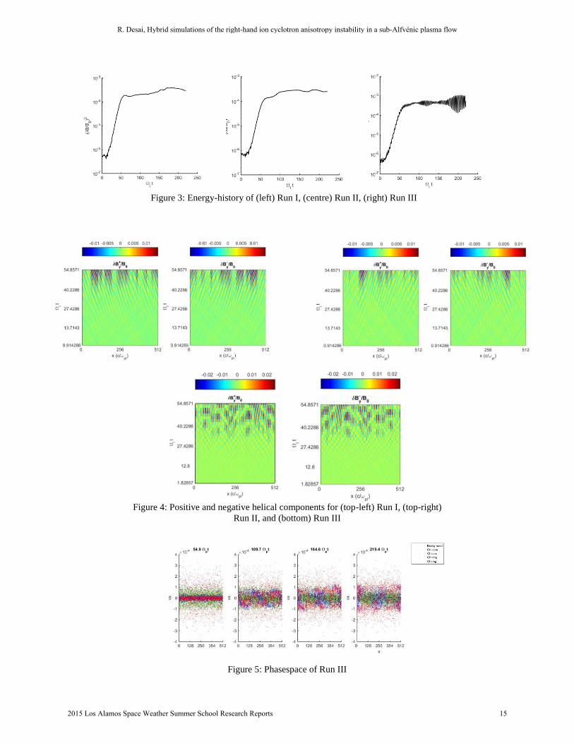
Figure 3: Energy-history of (left) Run I, (centre) Run II, (right) Run III

Figure 4: Positive and negative helical components for (top-left) Run I, (top-right)

Run II, and (bottom) Run III

Figure 5: Phasespace of Run III



Figure 6: Parametric study of the saturation energy dependence of the instability with respect to

variations in the pickup velocity and ring density



Abstract

Introduction


E. Hassan, A Statistical Ensemble for Solar Wind Measurement


Figure 1: Four Categories of Solar Wind origins in the Solar Corona. Adapted after Xu and Borovsky [2015]

Solar Wind Categorization Scheme

log10(υA) > 0.277log10(Sp) + 0.055log10(Texp/Tp) + 1.83

log10(Sp) > −0.525log10(Texp/Tp)− 0.676log10(υp) + 1.74

log10(Sp) < −0.658log10(υA)− 0.125log10(Texp/Tp) + 1.04



(a) Solar Maximum (2003)

(b) Solar Minimum (2008)

Figure 2: Testing solar wind data in OMNI dataset against 4-categorization scheme during (a) solar maximum and (b) solarminimum conditions. The wind categorizations are indicated in the figure legend.

Sp =Tp

n2/3p

, υA =B

(4πmpnp)1/2 , Texp = (υp

258)3.113

Solar Wind Advection



Figure 3: (a) Parker spiral model for the advection of magnetized plasma parcels in the solar wind, and (b) the probabilitydistribution function of the solar wind speed dependence on arrival angle at 1 AU.

tadv =(rs2 − rs2) · n

υsw · n(2)



.

Data Sources, Limitations, and Conditioning



Advected Solar Wind Parameters



(a) Data measured on July 21, 1998.

(b) Data measured on June 8, 2000.



Solar Wind Ensemble

∈



Figure 7: Uncategorized Kernel Density Estimation (KDE) functions of solar wind wind that are measured at IMP8 spacecraftbased on three years of advected measurements from ACE spacecraft to the IMP8 location using the flat-delay method.The vertical blue lines represent the interval of solar wind speeds measured at ACE.



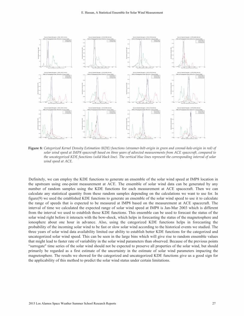
Figure 8: Categorized Kernel Density Estimation (KDE) functions (streamer-belt-origin in green and coronal-hole-origin in red) ofsolar wind speed at IMP8 spacecraft based on three years of advected measurements from ACE spacecraft, compared tothe uncategorized KDE functions (solid black line). The vertical blue lines represent the corresponding interval of solarwind speed at ACE.



Figure 9: An ensemble of solar wind speed at IMP8 location based on one-point of measurements at ACE spacecraft on Jan-Mar2003 by using the KDE functions generated for the solar wind data in 1998 - 2000.

Summary and Conclusions



Future Work

∈——————————————————

References

[1] MH Acuña, KW Ogilvie, DN Baker, SA Curtis, DH Fairfield, and WH Mish. The global geospacescience program and its investigations. Space Science Reviews, 71(1-4):5–21, 1995.

[2] Daniel N Baker. The occurrence of operational anomalies in spacecraft and their relationship to spaceweather. Plasma Science, IEEE Transactions on, 28(6):2007–2016, 2000.

[3] C Balch, B Murtagh, D Zezula, L Combs, G Nelson, K Tegnell, M Crown, and B McGehan. Serviceassessment: Intense space weather storms october 19–november 07, 2003. NOAA Silver Spring, Md,2004.

[4] EE Benevolenskaya and IG Kostuchenko. The total solar irradiance, uv emission and magnetic fluxduring the last solar cycle minimum. Journal of Astrophysics, 2013, 2013.



[5] RK Burton, RL McPherron, and CT Russell. An empirical relationship between interplanetary conditionsand dst. Journal of geophysical research, 80(31):4204–4214, 1975.

[6] Richard C Carrington. Description of a singular appearance seen in the sun on september 1, 1859.Monthly Notices of the Royal Astronomical Society, 20:13–15, 1859.

[7] Anthea Coster, John Foster, and Philip Erickson. Innovation-monitoring the ionosphere with gps-space weather-large gradients in the ionospheric and plasmapheric total electron content affects gpsobservations and measurements. gps data. GPS World, 14(5):42–49, 2003.

[8] James W Dungey. Interplanetary magnetic field and the auroral zones. Physical Review Letters, 6(2):47,1961.

[9] CJ Farrugia, FT Gratton, VK Jordanova, H Matsui, S Mühlbachler, RB Torbert, KW Ogilvie, andHJ Singer. Tenuous solar winds: Insights on solar wind–magnetosphere interactions. Journal ofAtmospheric and Solar-Terrestrial Physics, 70(2):371–376, 2008.

[10] HU Frey, TD Phan, SA Fuselier, and SB Mende. Continuous magnetic reconnection at earth’s magne-topause. Nature, 426(6966):533–537, 2003.

[11] SA Fuselier, KJ Trattner, and SM Petrinec. Antiparallel and component reconnection at the daysidemagnetopause. Journal of Geophysical Research: Space Physics (1978–2012), 116(A10), 2011.

[12] DK Haggerty, EC Roelof, CW Smith, NF Ness, RL Tokar, and RM Skoug. Interplanetary magneticfield connection to the l1 lagrangian orbit during upstream energetic ion events. Journal of GeophysicalResearch: Space Physics (1978–2012), 105(A11):25123–25131, 2000.

[13] TS Horbury, D Burgess, M Fränz, and CJ Owen. Prediction of earth arrival times of interplane-tary southward magnetic field turnings. Journal of Geophysical Research: Space Physics (1978–2012),106(A12):30001–30009, 2001.

[14] Michael C Kelley, Jonathan J Makela, Jorge L Chau, and Michael J Nicolls. Penetration of the solarwind electric field into the magnetosphere/ionosphere system. Geophysical Research Letters, 30(4), 2003.

[15] Margaret G Kivelson and Christopher T Russell. Introduction to space physics. Cambridge universitypress, 1995.

[16] Jeffrey J Love. Magnetic monitoring of earth and space. Physics Today, 61(2):31, 2008.

[17] B Mailyan, C Munteanu, and S Haaland. What is the best method to calculate the solar windpropagation delay? In Annales Geophysicae, volume 26, pages 2383–2394. Copernicus GmbH, 2008.

[18] Robert L McPherron, James M Weygand, and Tung-Shin Hsu. Response of the earth’s magnetosphereto changes in the solar wind. Journal of Atmospheric and Solar-Terrestrial Physics, 70(2):303–315, 2008.

[19] SE Milan, G Provan, and Benoît Hubert. Magnetic flux transport in the dungey cycle: A survey ofdayside and nightside reconnection rates. Journal of Geophysical Research: Space Physics (1978–2012),112(A1), 2007.

[20] Keith W Ogilvie, A Durney, and TT von Rosenvinge. Description of experimental investigations andinstruments for the isee spacecraft. IEEE Transactions on Geoscience Electronics, 16:151–153, 1978.

[21] Shinichi Ohtani, Teiji Uozumi, Hideaki Kawano, Akimasa Yoshikawa, Hisashi Utada, Tsutomu Nagat-suma, and Kiyohumi Yumoto. The response of the dayside equatorial electrojet to step-like changes ofimf bz. Journal of Geophysical Research: Space Physics, 118(6):3637–3646, 2013.



[22] Matt J Owens and Robert J Forsyth. The heliospheric magnetic field. Living Reviews in Solar Physics,10(5), 2013.

[23] Eugene N Parker. Dynamics of the interplanetary gas and magnetic fields. The Astrophysical Journal,128:664, 1958.

[24] KI Paularena and JH King. NasaâAZs imp 8 spacecraft. In Interball in the ISTP Program, pages 145–154.Springer, 1999.

[25] TI Pulkkinen, M Palmroth, EI Tanskanen, N Yu Ganushkina, MA Shukhtina, and NP Dmitrieva. SolarwindâATmagnetosphere coupling: a review of recent results. Journal of Atmospheric and Solar-TerrestrialPhysics, 69(3):256–264, 2007.

[26] IG Richardson, EW Cliver, and HV Cane. Sources of geomagnetic activity over the solar cycle: Relativeimportance of coronal mass ejections, high-speed streams, and slow solar wind. JOURNAL OFGEOPHYSICAL RESEARCH-ALL SERIES-, 105(A8):18–203, 2000.

[27] IG Richardson, EW Cliver, and HV Cane. Sources of geomagnetic storms for solar minimum andmaximum conditions during 1972–2000. Geophys. Res. Lett, 28(13):2569–2572, 2001.

[28] AJ Ridley. Estimations of the uncertainty in timing the relationship between magnetospheric and solarwind processes. Journal of Atmospheric and Solar-Terrestrial Physics, 62(9):757–771, 2000.

[29] CT Russell. Solar wind and interplanetary magnetic field: A tutorial. Space Weather, pages 73–89, 2001.

[30] CT Russell, JG Luhmann, and LK Jian. How unprecedented a solar minimum? Reviews of Geophysics,48(2), 2010.

[31] R Schwenn. Solar wind sources and their variations over the solar cycle. In Solar Dynamics and ItsEffects on the Heliosphere and Earth, pages 51–76. Springer, 2007.

[32] EC Stone, AM Frandsen, RA Mewaldt, ER Christian, D Margolies, JF Ormes, and F Snow. The advancedcomposition explorer. In The Advanced Composition Explorer Mission, pages 1–22. Springer, 1998.

[33] Daniel R Weimer and Joseph H King. Improved calculations of interplanetary magnetic field phasefront angles and propagation time delays. Journal of Geophysical Research: Space Physics (1978–2012),113(A1), 2008.

[34] DR Weimer, DM Ober, NC Maynard, WJ Burke, MR Collier, DJ McComas, NF Ness, and CW Smith.Variable time delays in the propagation of the interplanetary magnetic field. Journal of GeophysicalResearch: Space Physics (1978–2012), 107(A8):SMP–29, 2002.

[35] DR Weimer, DM Ober, NC Maynard, MR Collier, DJ McComas, NF Ness, CW Smith, and J Watermann.Predicting interplanetary magnetic field (imf) propagation delay times using the minimum variancetechnique. Journal of Geophysical Research: Space Physics (1978–2012), 108(A1), 2003.

[36] DT Welling. The long-term effects of space weather on satellite operations. In Annales Geophysicae,volume 28, pages 1361–1367. Copernicus GmbH, 2010.

[37] Daniel S Wilks. Statistical methods in the atmospheric sciences, volume 100. Academic press, 2011.

[38] Thomas N Woods. Irradiance variations during this solar cycle minimum. arXiv preprint arXiv:1003.4524,2010.

[39] Fei Xu and Joseph E Borovsky. A new four-plasma categorization scheme for the solar wind. Journal ofGeophysical Research: Space Physics, 120(1):70–100, 2015.

[40] L Zhao, TH Zurbuchen, and LA Fisk. Global distribution of the solar wind during solar cycle 23: Aceobservations. Geophysical Research Letters, 36(14), 2009.



Observations and Models of Substorm Injection Dispersion Patterns

Nadine M. E. Kalmoni

Mullard Space Science Laboratory, University College London, Dorking, RH5 6NT, UK

Michael G. Henderson

Los Alamos National Laboratory, New Mexico, US

Abstract

We present observations and models of a dispersionless substorm injection observed by Van Allen Probe A as it was

approaching apogee on 23 June 2013 at 05:24 UT. The injection was also observed from multiple geostationary Los

Alamos National Laboratory satellites. We compare enhancements in differential energy flux observed by multiple

spacecraft with dispersion signatures predicted by the Injection Boundary Model. By tracing particles backward in

time in steady state conditions we show whether or not a flux enhancement due to an injection is expected and if so,

what MLT location the particle originates from. This allows us localise the injection region radially as well as in MLT.

Keywords: substorm injections, dispersionless, dispersed, injection boundary model, Van Allen Probes, LANL

1. Introduction to Particle Motion in the Inner Magnetosphere

1.1. Single particle motion and particle drifts

Charged particles under the influence of electric and magnetic fields feel both the Coulomb force (due to the

electric field) and Lorentz force (due to the magnetic field). This gives the equation of motion for a charged particle

with charge q:

mdvdt= q(E + v × B) (1)

Gyro Motion

The Lorentz force acts perpendicular to the particle velocity, causing it to gyrate around a magnetic field line. If

the particle has a velocity component parallel to the magnetic field, then the particle will gyrate along the field line in

a helical trajectory. This allows us to define the particle pitch angle, α:

α = tan−1

(v⊥v‖

)(2)

where v⊥ and v‖ are the velocity components perpendicular and parallel to the magnetic field direction respectively.

The magnetic moment of a particle is given by the ratio between perpendicular energy and magnetic field strength. It

is also known as the first adiabatic invariant and is conserved over timescales longer than the particle gyro period.

μ =W⊥B=

mv2⊥2B=

mv2sin2α

2B(3)

Email addresses: [email protected] (Nadine M. E. Kalmoni), [email protected] (Michael G. Henderson)


Bounce Motion

If there is an increasing magnetic field strength along the field line, the parallel particle velocity component

decreases as the particle moves into a higher field strength. This corresponds to an increasing pitch angle. However

as no work is done on the particle the energy is conserved. This means that W⊥ increases and W‖ decreases. As μ is

conserved:

μ1 = μ2 =mv2sin2α1

2B1

=mv2sin2α2

2B2

(4)

sin2α2

sin2α1

=B2

B1

(5)

When the pitch angle becomes α = 90 the particle has no parallel energy and is reflected at its mirror point, Bm.

The magnetic mirroring of particles as they gyrate along the dipolar field lines in the Earth’s inner magnetosphere is

the cause of bounce motion.

Drift motion

If an electric field is present this introduces an additional particle drift across magnetic field lines. This is also

known as E × B drift and is perpendicular to both the electric and magnetic field and acts in the same direction for

both ions and electrons.

vE =E × B

B2

There are also particle drifts associated with a magnetic gradient or curvature of magnetic field lines.

A magnetic gradient leads to a drift perpendicular to both the magnetic field and its gradient.

v∇ =v2⊥

2qB3(B × ∇B)

The curvature of magnetic field lines causes a drift perpendicular to the radius of curvature and magnetic field.

vR =mv2‖

qRc × BR2

c B2

Equatorially mirroring particles do not feel the curvature drift as they do not have a velocity component parallel to

the magnetic field. Both the gradient and curvature drifts cause electrons to drift eastward and ions to drift westward.

This results in the ring current.

1.2. Adiabatic Invariants

The adiabatic invariants are treated as characteristic constants of particles, however they can change over long

time scales. Each of the particle motions outlined above has an adiabatic invariant associated with it:

• The first adiabatic invariant:

The magnetic moment, μ, is associated with gyration about the magnetic field.

• The second adiabatic invariant:

The longitudinal invariant, J, is associated with the motion along the magnetic field.

• The third adiabatic invariant:

Φ is associated with the drift motion perpendicular to the magnetic field.

N. Kalmoni, Observations and Models of Substorm Injection Dispersion Patterns


Figure 1: Particle drift paths for a) γμ = 0. Low energy particles of both species are dominated by electric field drifts. They have the stagnation

point at dusk. b) electrons with γμ = 0.05keV/γ. c) protons with γμ = 0.05keV/γ. (where γ = 1 × 10−9 T) (Kavanagh et al., 1968).

1.3. Drift Paths & Alfven layers

We have seen how electric and magnetic fields affect the particle trajectories. The magnetic field drifts are stronger

closer to Earth as the total magnetic field strength is higher. There are two different electric fields which also affect

particle motion due to E × B drift. This drift is not charge dependent and acts in the same direction for both ions and

electrons.

• Convection Electric Field

This dawn-dusk electric field is observed from the fixed frame of reference from the Earth due to solar wind

draping around the magnetosphere. The electric field is enhanced during a southward interplanetary magnetic

field (IMF) when the magnetosphere is in an ‘open’ configuration. The convection electric field dominates in

the tail, causing Earthward flow of plasma due to E × B drift.

• Corotation Electric Field

The corotation electric field is due to the rotation of the Earth and associated magnetic field lines which drag

the plasma with it due to the frozen- in condition. This is equivalent to an inward pointing electric field which

dominates over the convection electric field in the inner magnetosphere.

Taking into account all the electric and magnetic field drifts we can calculate the particle trajectories. These are

the same for zero energy particles of both species as the electric field drifts are not charge dependent. However for

non-zero energies the magnetic field drifts which are both energy and charge dependent cause differences between

electron and proton drift paths.

The overall particle drift is given by the following equation:

vd = vEcor + vEconv + v∇ + vR

This results in species and energy dependent particle trajectories. Particles which are far enough away from Earth

whose trajectories are dominated by the convection electric field are on open drift paths. Particles closer to Earth are

dominated by the corotation electric field and lie on closed drift paths. The boundary between the two region is called

the Alfven layer. Drift paths for different energy particles are shown in Figure 1. Figure 1a shows drift paths for low

energy electrons and protons. The Alfven layer stagnation point is located at dusk as this is whether the corotation and

convection drifts act in opposite directions and cancel out. Any particles inside the Alfven layer are stuck on closed

drift paths. For higher energy electrons the Alfven layer moves outwards. Higher energy protons have a stagnation

point on the dawn side as magnetic drifts act in the opposite direction to corotation.



Figure 2: a) Proposed double spiral injection boundary behind which all particles are energised at the time of injection (Mauk and Meng, 1983).

b) Injection boundary with colour coded MLT sections. The colours indicated are used to show the location of particle origin. If the initial particle

position in local time is: 18:00-20:00 yellow, 20:00-22:00 orange, 22:00-00:00 red, 00:00-02:00 green, 02:00- 04:00 light blue, 04:00-06:00 dark

blue (adapted from Mauk and Meng (1983)).

2. Introduction to Substorm Injections

Magnetospheric substorms are associated with multiple global and local signatures observed from the ground and

space. One signature of the substorm expansion phase is a sudden increase in particle fluxes over a wide energy range

observed from the nightside magnetosphere, usually from geosynchronous orbit (Konradi, 1967; Lanzerotti et al.,

1971; Belian et al., 1981). This is known as a substorm injection.

Substorm injections can be observed when the particles fluxes for multiple energy channels increase at the same

time i.e. dispersionless injections. If a satellite is in the injection region then the substorm injection will be disper-

sionless. However if the satellite is not in the injection region the particle fluxes will increase at different times. This

can be explained by particle drifts. Faster moving particles (higher energy) will arrive at the satellite earlier than low

energy particles. Arrival time also depends on the particle species and the location of the satellite in relation to the

injection region. Drift echoes can also be observed after injections if particles of certain energies lie on closed drift

paths at the satellite location.

The injection boundary model, is a phenomenological model used to predict the injection dispersion signatures

observed by satellites at geosynchronous orbit (McIlwain, 1974; Mauk and Meng, 1983). The model describes a

stationary boundary with the shape of a double spiral behind which protons and electrons of all energies are energised

at the same time. The boundary is shown in Figure 2a. If a satellite is located behind this boundary at the time

of injection a dispersionless injection is observed. A satellite which is not in the injection region will observed a

dispersed signature due to the different drift times and paths the energised particles follow after the injection.

In this study we investigate whether the injection boundary model and 90 pitch angle particle drifts due to a

Volland-Stern electric field and dipole magnetic field can explain substorm injection patterns observed by a satellite

in an eliptical orbit, e.g. Van Allen Probes. We investigate how the shape and orientation of the boundary affects

dispersion patterns and whether using multi-spacecraft measurements at geostationary orbit and the Van Allen Probes

allows us to localise the injection region in local time.



3. Instrumentation

3.1. Los Alamos National Laboratory Geostationary SatellitesThe Los Alamos National Laboratory (LANL) satellites are in a geostationary orbit.

The Magnetospheric Plasma Analyzer (MPA) consists of a single electrostatic analyser coupled to an array of channel

electro multipliers. It measures ion and electron energies in the range ∼ 1 eV/q to greater than 40 keV/q (Bame et al.,

1993).

The Synchronous Orbit Particle Analyzer (SOPA) consists of 3 solid state detector telescopes pointing at 30, 90 and

120 to the satellite’s spin axis. Differential fluxes of protons can be measured with energies from 50 keV to 50 MeV

and electrons from 50 keV to 1.5 MeV (Belian et al., 1992).

3.2. Van Allen ProbesFor this study we also use data from the Van Allen Probes Energetic Particle, Composition, and Thermal Plasma

Suite (ECT) . The Van Allen Probes mission consist of two probes, A and B, in elliptical orbits to study the radiation

belts with an apogee of 5.8 RE and orbital period of ∼ 9 hours.

The instruments used for this study are:

• Helium Oxygen Proton Electrion (HOPE) is an electrostatic top-hat analyser which measures electrons and ions

from below 20 eV (or spacecraft potential) to greater than 45 keV.

• Magnetic Electron Ion Spectrometer (MagEIS) measures electrons from 30 keV to 4 MeV and ions from 20

keV to 1MeV.

• Relativistic Electron Proton Telelscope (REPT) measures electrons from 4-10 MeV and protons from 20-75

MeV.

4. Observations

We present observations of a dispersionless substorm injection as observed at 05:24 UT by Van Allen Probe A

in Figure 3 on 23 June 2013. The top panel shows differential electron flux from the HOPE, MagEIS and REPT

instruments with increasing particle energy upwards on the y-axis. The second panel is the HOPE differential proton

flux with increasing particle energy downwards. This is so that the zero energy electrons and protons which follow

the same drift paths share a common axis. The third panel shows the MagEIS and REPT differential proton flux with

increasing particle energy downwards on the y-axis. In this plot the background flux has been removed in order to

show flux enhancements. Electrons and protons are energised up to 2 MeV in both species. Clear drift echoes are

then observed in the proton observations. This injection is shortly followed by a second injection at ∼ 06:00 UT. The

locations of the Van Allen Probes and geostationary LANL satellites at the time of the first injection are shown in

Figure 4.

5. Models of Substorm Injections based on the Injection Boundary Model

In order to investigate whether the injection boundary model can be used to explain the injection dispersion

pattern at multiple satellite locations, we trace protons and electrons with energies of 0 - 500 keV. This is done

from the satellite location at a time after the injection tracing backward to the injection time to find the particle

position of origin. If the location of the particle at the time of injection is on or tail ward of the injection boundary

then it is possible that the particle was energised due in the substorm injection. The particle tracing was done by

numerically solving the equation of motion (backwards in time) for equatorially mirroring particles in the guiding

centre approximation as given in Buzulukova et al. (2002):

drdt=

1

B · r ·[μ · ∂B∂φ

∣∣∣r +∂Φ

∂φ

∣∣∣r

](6)

dφdt= − 1

B · r ·[μ · ∂B∂r

∣∣∣φ+∂Φ

∂r

∣∣∣r

](7)



Figure 3: Dispersionless injection observed by Van Allen Probe A on 23 June 2013 at 05:24 UT. Top panel- detrended differential electron flux

observed form HOPE, MagEIS and REPT instruments. Middle two panels- detrended differential proton flux observed form HOPE, MagEIS and

REPT instruments. Note unconventional plot axes- electron energy increasing upwards and proton energy increasing downwards. Bottom panel-

satellite L-shell.



Figure 4: Locations of the LANL and Van Allen Probe satellites at the time of the substorm injection at 05:24 UT witha) an almost circular injection

boundary symmetric round 00:00 MLT, b) a more pronounced double spiral boundary rotated by π/4

where r and φ are the particle coordinates in the equatorial plane, μ is the particle magnetic moment divided by q, and

B is the dipole magnetic field strength in the equatorial plane. The electric potential is given by

Φ = −91.5 keV

r+ ΦCONV

where ΦCONV is the Volland-Stern electric field and is given in Ejiri (1978).

ΦCONV = ARγsinφ

where

A =0.045

(1 − 0.159Kp + 0.0093Kp2)3kV/R2

E

and the shielding factor, γ = 2 as proposed by Volland (1973) and Stern (1975).

If the particle traces back to the injection boundary it is colour coded depending on its MLT at the time of injec-

tion. The colours used are shown in Figure 2b.

Electrons and protons with energies 0 - 500 keV are traced back to the time of injection. If they originate from

behind the injection boundary they are coloured according to the MLT of their initial location. This is done for the

dispersion less injection observed by Van Allen Probe (VAP) A and is shown in Figure 5. At the time of injection VAP

A is located at ∼ 21:00 MLT. The models give a direct comparison with the observations, allowing us to determine

whether there are flux enhancements as expected due to an injection region spanning from dawn to dusk, or otherwise

a more localised injection region. The model shows that there is an instantaneous enhancement in particle flux from

the 20:00-22:00 MLT (orange) region at the time of the injection. This is because the satellite is in the injection

region at the time of injection. Shortly after high energy electrons from 18:00-20:00 MLT (yellow) are observed at

the satellite and high energy protons from 22:00-00:00 MLT (red) and 00:00-02:00 MLT (green). Drift echoes are

also predicted, but only clearly visible from observations in the proton data. The patterns observed as the satellite

travels back out to apogee on subsequent orbits is also visible. These are very similar to the structures observed in

the differential flux spectogram where protons with 10s keV arrive at the satellite before lower energy protons and

electrons, followed by electrons of a similar energy. This type of dispersion is visible in the observational data on the

second orbit after the injection. The first and second injection boundary topology gives very similar results for the

model, however the flux enhancement for the more rotated boundary lasts for a much longer time as the satellite is

located further tail ward of the boundary in this case.

The injection was also observed by other spacecraft located behind the injection region as shown in Figure 4.

The LANL-01A spacecraft which was located at ∼ 18:30 MLT also observed a dispersion less injection as shown in



Figure 6. This suggests that this satellite is also in the injection region, meaning that it spans at least form ∼ 18:30-

21:00 MLT. Again the flux enhancements in Figure 6e last longer than in c as the satellite is located further from the

boundary in this case. The two modelled dispersion patterns do not differ enough from each other to be able to deduce

whether the first or second injection boundary is more realistic.

Spacecraft 1994-084 was located at ∼ 02:00 MLT at the time of the injection. At this satellite no obvious flux

enhancement is observed, however according to Figure 7b the satellite is located behind the injection boundary and

therefore is expected to see a dispersionless injection. Even if the satellite is Earthward of the injection region we

would still expect to see a slightly dispersed signature shortly after the injection. From the data there is a flux

enhancement visible around the 100 keV electrons, however nothing at lower energies or in the proton data. The

model from the first injection boundary predicts a dispersion less injection at 05:24 UT from the 02:00-04:00 MLT

(light blue) region. This is clearly not visible in the observations. However the flux enhancement in high energy

electrons originates from the pre midnight 22:00-00:00 region. This suggests that particles in the post midnight region

behind the injection boundary are not energised. In order to test this the boundary was rotated in such a way that the

satellite was not behind the boundary at the time of injection. However the complex signature expected to be observed

at a later time in both electrons and ions from the 02:00-04:00 MLT region is not observed. This suggests that the

injection region in this case does not span from dawn to dusk and is more localised in MLT towards the pre-midnight

sector.

6. Conclusions & Further Work

From this study we can see that the patterns observed in low energy electron and proton Van Allen Probe data

in orbits after a substorm injection can be explained by simple particle drifts. The patterns observed differ from the

models due to the steady-state conditions used to run the model. In reality the strength of the convection electric field

changes on shorter timescales. In our example the influence of a substorm injection can be measured in the inner

magnetosphere up to two orbits later.

Using measurements from multiple spacecraft it is possible to narrow down the MLT width of the injection region

for individual events and compare the differential flux enhancements and dispersion patterns with those predicted by

particle drifts. These methods can also allow future investigations into the shape of the injection region, whether it

is centred around midnight, and how far behind the injection region the particles are energised. Future work on this

subject includes:

• Investigating the shape of the injection boundary and the effect on the expected dispersion pattern. This can

include how important a rounded/spiral injection boundary is to reproduce observations.

• It is unclear how much the width of the energisation behind the injection boundary affects dispersion patterns.

• The effect of rotating the boundary on the dispersion patterns

• Testing the consistency between observations of injections and the results from the model.

References

Bame, S.J., McComas, D.J., Thomsen, M.F., Barraclough, B.L., Elphic, R.C., Glore, J.P., Gosling, J.T., Chavez, J.C., Evans, E.P., Wymer, F.J.,

1993. Magnetospheric plasma analyzer for spacecraft with constrained resources. Review of Scientific Instruments 64, 1026–1033.

Belian, R.D., Baker, D.N., Hones, E.W., Higbie, P.R., Bame, S.J., Asbridge, J.R., 1981. Timing of energetic proton enhancements relative to

magnetospheric substorm activity and its implication for substorm theories. Journal of Geophysical Research: Space Physics 86, 1415–1421.

Belian, R.D., Gisler, G.R., Cayton, T., Christensen, R., 1992. High-z energetic particles at geosynchronous orbit during the great solar proton event

series of october 1989. Journal of Geophysical Research: Space Physics 97, 16897–16906.

Buzulukova, N.Y., Galperin, Y.I., Kovrazhkin, R.A., Glazunov, A.L., Vladimirova, G.A., Stenuit, H., Sauvaud, J.A., Delcourt, D.C., 2002. Two

types of ion spectral gaps in the quiet inner magnetosphere: Interball-2 observations and modeling. Annales Geophysicae 20, 349–364.

Ejiri, M., 1978. Trajectory traces of charged particles in the magnetosphere. Journal of Geophysical Research: Space Physics 83, 4798–4810.

Kavanagh, L.D., Freeman, J.W., Chen, A.J., 1968. Plasma flow in the magnetosphere. Journal of Geophysical Research 73, 5511–5519.

Konradi, A., 1967. Proton events in the magnetosphere associated with magnetic bays. Journal of Geophysical Research 72, 3829–3841.

Lanzerotti, L.J., Maclennan, C.G., Robbins, M.F., 1971. Proton drift echoes in the magnetosphere. Journal of Geophysical Research 76, 259–263.

Mauk, B.H., Meng, C.I., 1983. Characterization of geostationary particle signatures based on the injection boundary model. Journal of Geophysical

Research: Space Physics 88, 3055–3071.



McIlwain, C.E., 1974. Substorm injection boundaries, in: McCormac, B.M. (Ed.), Magnetospheric Physics, pp. 143–154.

Stern, D.P., 1975. The motion of a proton in the equatorial magnetosphere. Journal of Geophysical Research: Space Physics 80, 595–599.

Volland, H., 1973. A semiempirical model of large-scale magnetospheric electric fields. Journal of Geophysical Research: Space Physics 78,

171–180.



Figure 5: a) Detrended differential electron and proton flux on 23 June 2013 for Van Allen Probe A which is at ∼ 21:00 MLT at the time of injection. The dispersionless injection is visible at 05:24UT. b) The injection boundary used for the modelled dispersion pattern in c). c) The modelled dispersion pattern where the colours indicate whether a particle from the injection region has access to the satellite at a particular time and if so, the MLT sector from which the particle originates. d) The double spiral rotated by π/4 injection boundary used in e) for the modelled dispersion pattern. e) The modelled dispersion pattern using a rotated injection boundary. The axes for the observations and models are in the same layout as Figure 3.



Figure 6: a) Detrended differential electron and proton flux on 23 June 2013 for LANL-01A which is at ∼ 18:30 MLT at the time of injection. At this satellite a dispersionless injection is also observed at 05:24 UT. b) The injection boundary used for the modelled dispersion pattern in c). c) The modelled dispersion pattern where the colours indicate whether a particle from the injection region has access to the satellite at a particular time and if so, the MLT sector from which the particle originates. d) The double spiral rotated by π/4 injection boundary used in e) for the modelled dispersion pattern. e) The modelled dispersion pattern using a rotated injection boundary. The axes for the observations and models are in the same layout as Figure 3.



Figure 7: a) Detrended differential electron and proton flux on 23 June 2013 for 1994-084 which is located at ∼ 02:00 MLT at the time of injection. At this satellite no obvious flux enhancement is observed at the time of injection even though the spacecraft is located behind the injection boundary dispersion less injection is expected. b) The injection boundary used for the modelled dispersion pattern in c). c) The modelled dispersion pattern where the colours indicate whether a particle from the injection region has access to the satellite at a particular time and if so, the MLT sector from which the particle originates. d) The double spiral rotated by π/4 injection boundary used in e) for the modelled dispersion pattern. e) The modelled dispersion pattern using a rotated injection boundary. The axes for the observations and models are in the same layout as Figure 3.



Heavy Ion Effects on Kelvin-Helmholtz Instability: Hybrid Study

Dong Lin

Department of Electrical & Computer Engineering, Virginia Polytechnic Institute and State University, Blacksburg, VA.

Misa Cowee, Dan Winske, Xiangrong Fu

Los Alamos National Laboratory, Los Alamos, NM

Abstract

We investigated the effects of heavy ions on the Kelvin-Helmholtz instability (KHI) via hybrid simulation. In a two-

dimensional setup, the density and temperature is uniform across the shear layer. The magnetic field is also uniform

and perpendicular to the simulation plane. The heavy ion effects are explored by varying the mass number of the

ion species while keeping the mass density constant for four simulation runs. The mass numbers involved are 1,

4, 8 and 16. By doing spatial Fourier analysis for the perpendicular velocity disturbance on the central line of the

simulation box, we characterized the growth rate of the KH instability for different wave mode numbers. The wave

mode dependent growth rate is compared with theoretical predictions and good agreement is found. Comparison of

growth rates for different ion species shows the instability grows slower with a heavier ion species. Possible influences

of shear layer thickness, system size, and grid spacing are discussed.

Keywords: Kelvin-Helmholtz Instabiltiy, Heavy Ion, Hybrid Simulation

1. Introduction

KHI is also called the “wind-blow-water instability” in fluid dynamics, which occurs on the interface of two fluids

when there is a strong velocity shear. Such a strongly sheared interface is also present in space plasma, which is

often characterized by magnetohydrodynamics (MHD). KHI is suggested as a candidate mechanism in solar wind-

magnetosphere coupling and contributes to the transport of solar wind mass, momentum and energy into the magneto-

sphere (Hasegawa et al., 2004). An early estimation by Pu and Kivelson (1983) shows that the energy power supplied

to the magnetosphere by KHI is only next to that by magnetic reconnection and preponderates over other mechanisms

like diffusion, injection, etc.

The linear MHD theory of Chandrasekhar (1961) gives the unstable criteria:

[k · (V1 − V2)]2 >ρ1 + ρ2

μ0ρ1ρ2

[(k · B1)2 + k · B2)2] (1)

and the growth rate on an infinitely thin shear layer:

γ =

√ρ1ρ2

(ρ1 + ρ2)2[k · (V1 − V2)]2 − ρ1

ρ1 + ρ2

(k · VA1)2 − ρ2

ρ1 + ρ2

(k · VA2)2 (2)

where the subscripts “1” and “2” denote the velocity, mass density, and magnetic field at the two sides of the shear

layer. From the unstable criteria we see that the most unstable condition is when the magnetic field is perpendicular

to the velocity shear. Based on the frame work of MHD, Miura and Pritchett (1982) did eigen-mode analysis for

the instability growth rate dependence on the wave number. Figure 1 gives the result for the case of magnetic field

Email address: [email protected] (Dong Lin)


Figure 1: Normalized growth rate dependence on the normalized wavenumber for inverse magnetosonic Mach numbers ranging from 0.6 to ∞from the eigen-mode analysis of Miura and Pritchett (1982).

Table 1: Parameters of the hybrid simulation

n0 B0 Ti = Te βi = βe ω−1ci l0 = c/ωci VA

5cm−3 20 nT 10 eV 0.05 0.5 s 101 km 195 km/s

Grids NPPC Size η dt 2a V0

5122 200 (160l0)2 10−4 0.05 ω−1ci 2.0l0 1.0VA

perpendicular to the velocity with different magnetosonic Mach numbers. The fastest growing mode generally falls in

the range of

0.5 < k · 2a < 1.0 (3)

where k · 2a is the wavenumber k normalized by the initial shear width 2a. The growth rate γ is normalized by 2a/V0,

where V0 is the total velocity shear.

The KHI has been frequently seen in the observations of diverse spacecraft. The statistical study of Lin et al.(2014) shows the occurrence of KHI on the magnetopause from the dayside to the nightside. At the same time, heavy

ions are also reported to dominate the magnetopause for as much as 30% of the time on the dusk side (Bouhram etal., 2005). Possible sources of these heavy ions include O+ from the ionospheric outflow, He++ and other ion species

from the solar wind, and so on.

The MHD theory does not include any ion effects and the growth rate appears to be the same for different ion

species. Previous studies on the possible influences of heavy ions have not yet come to an agreement. On one hand,

the heavy ions will contribute to a higher mass density, and thus lower the Alfven speed and reduce the magnetic

tension effects. The instability threshold is supposed to decrease (e.g., Johnson et al., 2009; Yu and Ridley, 2013).

On the other hand, heavy ions have stronger inertial effects as single particles. They are thought to be able to stream

through the KH vortices and break them down. Consequently, the instability is likely to be suppressed and mixing

reduced (e.g., Delamere et al., 2011; Merkin, 2011). With these competing hypotheses, it naturally raises the question:

do heavy ions promote or inhibit the KH instability?

2. Methodology

Since we are interested in the potential ion effects, the hybrid model in which ions are treated as particles and

electrons as massless fluid (Winske et al., 2003) would be an appropriate method. The hybrid simulation could study

phenomena on the spatial scale of ion inertial length and gyro-radius with a low frequency approximation for the

D. Lin, Heavy Ion Effects on Kelvin-Helmholtz Instability: Hybrid Study


electromagnetic fields. Here are the basic equations for the hybrid model (Winske and Omidi, 1993):

∇ × B = 4π

cJ (4)

∇ × E = −1

c∂B∂t

(5)

∇ · B = 0 (6)

∂

∂tnemeVe = 0 = −ene(E +

Ve × Bc

) − ∇· ↔Pe +ene↔R · J (7)

dxi

dt= vi (8)

midvi

dt= qi(E +

vi × Bc

) − qiη J (9)

The pressure and resistivity tensor are simplified as isotropic. The electron and ion number density are connected by

the charge neutrality condition, namely we do not solve the Poisson’s equation in this hybrid model. Thus we have

the following additional equations:

↔Pe= neTe

↔I (10)

↔R= η

↔I (11)

niqi = neqe (12)

J = neqe(Vi − Ve) (13)

In this summer program, we started with the simplest situation of two-dimensions with only one ion species

involved in each run. The mass density is uniform across the shear layer and kept as a constant for different runs. The

magnetic field is set to be perpendicular to the simulation plane, which is the most unstable configuration as discussed

before. The boundary is periodic in the flow direction Y and reflecting in the other direction X. Typical values in

spacecraft observations are adopted for the plasma and magnetic field, as shown in Table 1. The simulation system

size is 160l0 × 160l0, where l0 is the ion inertial length, with 512 × 512 grid cells. The number of super particles per

cell is 200. We use a numerical resistivity of η = 10−4 and time step of 0.05ω−1ci , where ω−1

ci is the inverse of ion gyro

frequency. The shear width is 2l0 and velocity shear is 1.0VA, where VA is the plasma Alfven speed. In the shear layer,

the transition of shear velocity is proscribed by the typical hyperbolic tangent function:

VY =V0

2tanh(

Xa

) (14)

Figure 2: Velocity profile at the initial time.



3. Results

3.1. The case of protonsWe started with the most fundamental ion species: protons. Figure 2 shows the flow velocity profile in the

beginning of the simulation. The dash lines denote the nominal width of the shear layer. Figure 3 gives the simulation

Figure 3: Density contour and flow field at t = 150ω−1ci .

result of KHI for protons. The top left panel gives the density contour and flow field at t = 150ω−1ci for ions initially

located at the left side of the shear layer, and top right panel for ions initially at the right. The bottom panel plots

the total density and velocity distribution. About eight KH vortices can been seen from the density contour. The

coalescence of vortices to larger ones is also evident. In order to quantify the growth rate of the instability, a spatial

Figure 4: Temporal evolution of the spatial Fourier spectrum of perpendicular velocity disturbance at X = 0.

Fourier transform is performed for the perpendicular velocity disturbance on the central line of the simulation domain.



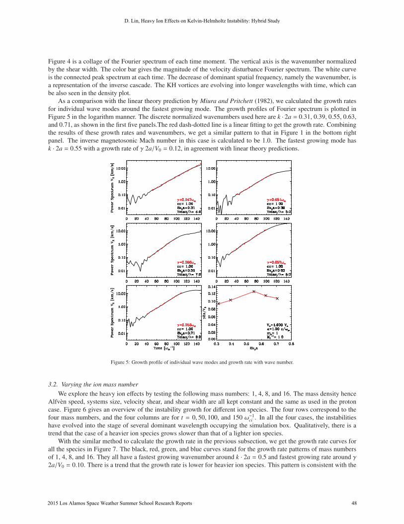
Figure 4 is a collage of the Fourier spectrum of each time moment. The vertical axis is the wavenumber normalized

by the shear width. The color bar gives the magnitude of the velocity disturbance Fourier spectrum. The white curve

is the connected peak spectrum at each time. The decrease of dominant spatial frequency, namely the wavenumber, is

a representation of the inverse cascade. The KH vortices are evolving into longer wavelengths with time, which can

be also seen in the density plot.

As a comparison with the linear theory prediction by Miura and Pritchett (1982), we calculated the growth rates

for individual wave modes around the fastest growing mode. The growth profiles of Fourier spectrum is plotted in

Figure 5 in the logarithm manner. The discrete normalized wavenumbers used here are k · 2a = 0.31, 0.39, 0.55, 0.63,

and 0.71, as shown in the first five panels.The red dash-dotted line is a linear fitting to get the growth rate. Combining

the results of these growth rates and wavenumbers, we get a similar pattern to that in Figure 1 in the bottom right

panel. The inverse magnetosonic Mach number in this case is calculated to be 1.0. The fastest growing mode has

k · 2a = 0.55 with a growth rate of γ 2a/V0 = 0.12, in agreement with linear theory predictions.

Figure 5: Growth profile of individual wave modes and growth rate with wave number.

3.2. Varying the ion mass numberWe explore the heavy ion effects by testing the following mass numbers: 1, 4, 8, and 16. The mass density hence

Alfven speed, systems size, velocity shear, and shear width are all kept constant and the same as used in the proton

case. Figure 6 gives an overview of the instability growth for different ion species. The four rows correspond to the

four mass numbers, and the four columns are for t = 0, 50, 100, and 150 ω−1ci . In all the four cases, the instabilities

have evolved into the stage of several dominant wavelength occupying the simulation box. Qualitatively, there is a

trend that the case of a heavier ion species grows slower than that of a lighter ion species.

With the similar method to calculate the growth rate in the previous subsection, we get the growth rate curves for

all the species in Figure 7. The black, red, green, and blue curves stand for the growth rate patterns of mass numbers

of 1, 4, 8, and 16. They all have a fastest growing wavenumber around k · 2a = 0.5 and fastest growing rate around γ2a/V0 = 0.10. There is a trend that the growth rate is lower for heavier ion species. This pattern is consistent with the



Figure 6: KHI growth for different ion species: mass number M = 1, 4, 8, 16.

result of Case 3 in Delamere et al. (2011) although the dependence of growth rate on wavenumber is not discussed in

that study.

3.3. Additional sensitivity tests

Before we attempt to find a physical explanation for the growth rate pattern found above, we did several more

sensitivity tests of growth rate to the shear width, grid spacing, and system size. In a simulation box of 80l0 × 80l0,

we vary the shear width 2a among 0.32, 0.62, 1.24, 2.00, to 4.00. The corresponding growth rate curves are shown

in Figure 8 with black, red, green, blue, and yellow, respectively. Note the legend in Figure 8 is for half shear width

a. Only when 2a = 1.24, 2.00 can we see a growth rate curve close to the prediction. For too wide or too narrow

shear width, the fastest growing mode and growth rate are much deviated from the predicted value. For the too narrow

case, for example 2a = 0.32, the shear width is just around one grid cell. The transition of shear velocity would be

too abrupt on the grids. For too wide shear width in a given system size, the limiting effects of the boundaries in the

perpendicular direction may come out. Thus it is necessary to find out the appropriate range of shear width given the

system size of a simulation box.



Figure 7: KHI growth rate with wavenumber for different ion species: mass number M = 1, 4, 8, 16.

Figure 8: KHI growth rate with wavenumber

for different shear widths: a = 0.16 (black),

0.31 (red), 0.62 (green), 1.00 (blue), and 2.00

(yellow).

Figure 9: KHI growth rate with wavenum-

ber for different grid spacings: dx = 0.6250

(black), 0.3125 (red), and 0.1562 (green).

Figure 10: KHI growth rate with wavenum-

ber for different system sizes: Xmax = 40 l0(black), 80 l0 (red), and 160 l0 (green).

The grid spacing and system size give the lower and upper limit of wavelength that could be resolved. In a system

size of 80 l0 × 80 l0, we tested the effects of grid spacing by varying the number of grid cells from 1282, 2562 to 5122,

shown by the black, red, and green curves, respectively in Figure 9. The black and green dashed lines are when the

number of super particles per cell is 400 for dx = 0.6250 and 100 for dx = 0.1562 so that the total number of super

particles is all the same for three grid spacings. It is found that the growth rate for a larger grid spacing is relatively

lower. The number of super particles per cell does not produce significant changes. This could result from that more

short wavelength modes are cut off by a larger grid cell, thus reducing the number of seeds for the instability growth,

or could be due to numerical effects associated with the initial conditions.

In another sensitivity test, the system size Xmax is the only variable: 40 l0 × 40 l0, 80 l0 × 80 l0, 160 l0 × 160 l0.

The growth rate curves are basically unchanged, which maybe because the instability has not evolved to a wavelength

comparable to the system size by the time the growth rate is calculated.



4. Summary

In this study, we use the hybrid model to simulate the KHI for different ion species. The growth rate dependence

on wavenumber is in good agreement with the linear theory prediction of Miura and Pritchett (1982). As the mass

number of the ions increases to 4, 8, and 16, the growth rate appears to decrease. The test runnings show that instability

growth is also sensitive to the shear width, grid spacing. Although variations of growth rate caused by shear width

and/or grid spacing may be attributed to numerical effects, it is necessary to have more tests to validate the outcomes

for further study.

The linear theory of Miura and Pritchett (1982) is essentially based on the frame work of MHD. It is important to

derive the linear theory for kinetic KHI in the future research. Full particle simulations of Nakamura et al. (2010) have

shown that the shear layer is prone to broaden if the initial width is comparable to or less than one ion gyro-radius

when the vorticity of shear flow is anti-parallel to the magnetic field. It is thus noteworthy if these broadening effects

are strengthened by the presence of a heavier ion species, whose gyro-radius is larger. We have not considered the

magnetic shear in this study. When the instability is stabilized by the parallel magnetic tension, the difference between

ion species may stand out. Thus runs with a finite magnetic shear are suggested for future work to provide helpful

hints for the investigation of heavy ion effects on the Kelvin-Helmholtz instability.

5. References

Bouhram, M., B. Klecker, G. Paschmann, and et al. (2005), Survey of energetic O+ ions near the dayside mid-latitude magnetopause with Cluster,

Ann. Geophys., 23, 1281–1294

Chandrasekhar, S. (Ed.) (1961), Hydrodynamic and Hydromagnetic Stability, Oxford Univ. Press, New York.

Delamere, P. A., R.J.Wilson, A. Masters, Kelvin-Helmholtz instability at Saturn’s magnetopause: hybrid simulations, J. Geophys. Res., 116, 10222,

doi:10.1029/2011JA016724.

Hasegawa, H., M. Fujimoto, T. D. Phan, and et al. (2004), Transport of solar wind into Earth’s magnetosphere through rolled-up Kelvin-Helmholtz

vortices, Nature, 430(7001), 755–758, doi:10.1038/nature02799.

Johnson, J., A. Otto, Y. Lin, and et al. (2009), Heavy ion effects on magnetopause transport, AGU FallMeeting Abstracts, 2

Lin, D., C. Wang, W. Li, and et al. (2014), Properties of Kelvin-Helmholtz waves at the magnetopause under northward interplanetary magnetic

field: Statistical study, J. Geophys. Res., 119, 7485–7494, doi:10.1002/2014JA020379.

Merkin, V. G., Effects of ionospheric O+ on the magnetopause boundary wave activity, American Institute of Physics Conference Series, ed. by D.

Vassiliadis et al., 1320, 208–212, doi:10.1063/1.3544326.

Miura, A., and P. L. Pritchett (1982), Nonlocal stability analysis of the MHD Kelvin-Helmholtz instability in a compressible plasma, J. Geophys.Res., 87(A9), 7431–7444, doi:10.1029/JA087iA09p07431.

Nakamura, T. K. M., H. Hasegawa, I. Shinohara (2010), Kinetic effects on the Kelvin-Helmholtz instability in ion-to-magnetohydrodynamic scale

transverse velocity shear layers: particle simulations, Phys. Plasmas, 17(4), 042119. doi:10.1063/1.3385445.

Pu, Z. Y., and M. G. Kivelson (1983), Kelvin-Helmholtz instability at the magnetopause: Solution for compressible plasmas, J. Geophys. Res.,88(A2), 841–852, doi:10.1029/JA088iA02p00841.

Winske, D., and N. Omidi (1993), Hybrid codes. Computer space plasma physics: Simulation techniques and software, 103–160.

Winske, D., L. Yin, N. Omidi, and et al. (2003), Hybrid simulation codes: past, present and future-a tutorial, Space Plasma Simulation, 136–165,

Springer Berlin Heidelberg.

Yu, Y., and A.J. Ridley (2013), Exploring the influence of ionospheric O+ outflow on magnetospheric dynamics: the effect of outflow intensity, J.Geophys. Res., 118, 5522–5531, doi:10.1002/jgra.50528.



Simulating Plasmaspheric Electron Densities with a Two-Component

Electric Field Model

Sebastian De Pascuale

Department of Physics & Astronomy, University of Iowa, Iowa City, IA, 52242

Vania Jordanova

Los Alamos National Laboratory, Los Alamos, NM 87545

Abstract

We simulate equatorial plasmaspheric electron densities in the inner-magnetosphere with a fluid-physics model

(RAM-CPL) based on empirical parameters governing the source and loss processes of refilling and erosion. A virtual

plasmasphere is compared with Van Allen Probe (RBSP-A) EMFISIS density measurements along the orbital track

of the satellite on 15 - 20 January, 2013. The evolution of the simulation is driven by a combined Volland-Stern

and SAPS electric potential, parameterized by solar wind measurements and the Kp index respectively to account

for the convection of plasma in the inner-magnetosphere. Globally, the simulations indicate the compression of the

plasmapause boundary, defined as a low-density threshold of 20 cm−3, to L = 4 and the narrowing of a plume-

like structure of plasma during the onset of geomagnetic activity, which is consistent with other modeling efforts.

Locally, the RAM-CPL simulation achieves favorable agreement within an order of magnitude of EMFISIS density

measurements and a mean model-observation difference in plasmapause detections of ΔLAVG = 0.52 ± 0.15RE . We

discuss further the effects of EMFISIS density determinations and the parameterization of the convection electric field

on this reported disagreement.

Keywords: plasmaspheric erosion & refilling, convection electric field, Van Allen Probes, RBSP, EMFISIS, EFW

1. Introduction

Entrained by Earth’s dipolar magnetic field and subsequently corotating with the planet, the plasmasphere is a

toroidal interface of cold, dense plasma (≤ 20 eV, 10 − 104 cm−3, and primarily H+) coupled to the ionosphere and

inner-magnetosphere (Lemaire and Gringauz, 1998). Dayside magnetic reconnection at the the magnetopause drives

the sunward convection of near-Earth plasma caused by a duskward electric field, which contributes to the erosion of

the plasmasphere and related dynamics on the order of hours during periods of geomagnetic activity (Carpenter and

Lemaire, 1997). The time history of a geomagnetic storm further influences the formation of plume-like structures and

other morphological features of the plasmasphere (Goldstein and Sandel, 2005; Darrouzet et al., 2009). Plasmaspheric

drainage plumes, in particular, can interact with and modify regions of magnetic reconnection as they channel escaping

plasma towards the magnetopause (Walsh et al., 2014). Nonetheless, the origin of plasma sustaining long-lived

plumes is unknown, requiring full-scale simulations and further work to uncover the role of the plasmasphere on inner

magnetospheric processes (Borovsky et al., 2014).

During periods of extended geomagnetic inactivity (Kp < 2), the plasmasphere refills more effectively from the

continual supply of particles escaping from the dayside ionosphere (Darrouzet et al., 2009). Outflow along co-rotating

flux tubes, dominated by the charge exchange reaction liberating H+ protons, returns the plasmasphere to an extended

state on a timescale of days that is dependent inversely on ionospheric latitude or inner-magnetospheric L-shell (Ras-

mussen et al., 1993). The outer boundary of the plasmasphere, the plasmapause, is identified as a discontinuity in the

Email addresses: [email protected] (Sebastian De Pascuale), [email protected] (Vania Jordanova)


radially decaying profile describing equatorial densities, and its location (from 3 < L < 8 ) is inversely dependent on

geomagnetic activity and well described by E x B convection models (Carpenter and Anderson, 1992; Goldstein et

al., 2005). Specification of the forcing electric field can include modifications to simple convection from electromag-

netically coupled plasma and particle populations in the ionosphere and inner-magnetosphere.

The subauroral polarization stream (SAPS) phenomenon, for example, arises from a global electrical circuit be-

tween the partial ring current during disturbance times and field-aligned and poleward Pedersen currents in the iono-

sphere. When this feedback effect is mapped from ionospheric latitudes to the inner-magnetosphere, SAPS accounts

for radial electric fields producing westward flows in the plasmasphere (Goldstein et al., 2005). Thermal plasma

density content in the plasmasphere is responsible for the collisional loss of ions and host to the plasma waves that

scatter electrons from the surrounding hot (>1 keV) ring current and (>1 meV) radiation belts (Lyons, et al. 1998;

Fok, et al. 1991; and Jordanova et al., 1996). The advanced ring-current atmosphere interaction and radiation belt

model (RAM-SCB) is coupled to a time-dependent equatorial plasmaspheric density model (RAM-CPL; cold plasma)

to study the acceleration, transport, and loss of energetic electrons and ions in the inner magnetosphere, a prime sci-

entific objective of the recently completed main Van Allen Probes mission (Jordanova and Miyoshi 2005; Jordanova

et al., 2010a, 2010b).

Formerly known as the Radiation Belt Storm Probes (and hereafter as RBSP-A & -B), the presently orbiting Van

Allen Probes mission is providing a detailed perspective of the relationship between the plasma populations of the

radiation belts, ring current, and plasmasphere. At near equatorial ( 10) geostationary transfer orbits (period 9h), the

two lapping satellites extend from a perigee of 600 km to an apogee of 5.8 RE . Measurements of the electromagnetic

environment allow direct contextualization of particle observations and associated plasma waves. The Electric Field

and Waves (EFW) instrument (Wygant et al., 2013) measures three-axis electric fields driving the system and the

spacecraft potential that serves as a proxy of the ambient plasma density. A reliable determination of the electron

number density is obtained from frequency signatures in spectral data captured by the Electric and Magnetic Field

Instrument Suite and Integrated Science (EMFISIS) suite (Kletzing et al., 2013; Kurth et al., 2015). These local in situ

measurements can be compared to global models of the equatorial plasmasphere in order to constrain the dependence

of its behavior on key variables.

Promoted by a host of specialized missions (multipoint, sounding, and imaging), the last decade of plasmaspheric

research has focused on developing better understanding of the influence of geomagnetic events on the plasmasphere

as a two-way coupling problem between the magnetosphere-plasmasphere and plasmasphere-ionosphere (Ganguli et

al., 2000). Early empirical work utilized the identification of the plasma oscillation frequency, similar to the EMFISIS

method (Kurth et al., 2015), to determine electron density profiles of half (00-15 hrs; Carpenter and Anderson, 1992)

and full (00-24 hrs; Sheeley et al., 2001) MLT coverage. Recent analysis demonstrates that conventional empirical

models fall short of reproducing observations when compared to direct in situ measurements, indicating that the

ambient electron density of the plasmasphere is a critical parameter to theoretical wave and particle investigations (Ni

et al., 2013; Thorne et al., 2013).

In this paper we assess the performance of equatorial plasmaspheric electron density simulations produced by

RAM-CPL (cold plasma), a coupled component of the newly-developed RAM-SCB (eg. Jordanova et al., 2006). We

consider two geomagnetic events on 15 - 20 January and 31 May - 5 June, 2013 during Van Allen Probes observations

separated by a quarter sector in MLT from pre- to post-midnight regions. Although the initial and steady-state con-

ditions of this study are static, the simulations are driven by an empirical description of the convection electric field

chosen to reflect two distinct processes: magnetospheric dayside reconnection and sub global current system feed-

back in the ionosphere. We use the Kp geomagnetic activity index to parameterize the evolution of the plasmasphere

and define a plasmapause boundary to systematically contextualize actual and virtual observations. For both events,

the agreement in plasmapause location of the encounters was reproduced to within 0.50 Re. As the mean separation

between spacecraft during both of these events is ∼ .5 L, we present simulation comparisons at a resolution of .5 hr

MLT by 0.25 L bins against RBSP-A only, and for brevity will discuss only the results from the 15 - 20 January, 2013

event.

The subsequent sections of this paper are organized in the following manner: we describe the RAM-CPL modeling

scheme used in this study and the representations for the source and loss processes of refilling and erosion, then

we highlight density features of the EMFISIS observations captured by the simulation, and close by presenting an

assessment of using RAM-CPL to provide plasmapause locations as a threshold in density. Future work will be

discussed following a summary of the results of this study.

S. De Pascuale, Simulating Plasmaspheric Electron Densities with a Two-Component Electric Field Model


2. Modeling Framework

We ran two simulations of the ring-current atmosphere interaction cold plasma (RAM-CPL) in order to validate

empirical models describing convective erosion and ionospheric refilling of the plasmasphere when compared to

measurements obtained by the Van Allen Probes. A series of similar studies carried out by Liemohn et al. (2004,

2005, and 2006) linked RAM to the Dynamic Global Core Plasma Model (DGCPM; Ober et al. 1997) and found

that coupling to the ring current and ionosphere for calculation of a self-consistent inner magnetospheric electric field

better reproduced plasmapause locations as extracted from IMAGE EUV observations. DGCPM, while solving for

total magnetic flux tube density content by a continuity equation in the same manner as RAM-CPL, is developed

separately to be integrated with arbitrary magnetic and electric field specifications as well as to be coupled to other

codes (Chen and Wolf, 1972; Rasmussen et al., 1993). We study RAM-CPL, which can also specify an arbitrary

electric field, as a subroutine of the existing RAM suite to assess its utility in describing inner-magnetospheric cold

plasma.

The two-dimensional equatorial plasmaspheric electron density model of RAM-CPL (illustrated in Figure 1)

incorporates a parametric function of particle refilling due to ionosphere-magnetosphere coupling during E x B plas-

maspheric evolution (Rasmussen et al., 1993). Two empirically derived components, a static refilling rate and a

time-dependent driver, are utilized to dynamically progress the simulated configuration of plasma through the ob-

served history of a geomagnetic event. The simulation will be compared to RBSP-A EMFISIS measurements by

flying a virtual satellite through its orbit in the model plasmasphere output to record electric field and electron density

values. A detailed examination of the role of a duskward electric field on ring current and plasmasphere formation

for the 31 May - 5 June, 2013 storm is carried out by the work Thaller et al., 2015, which indicates that the EFW

measured enhanced electric field is coincident with plasmasphere erosion. As an additional metric of comparison,

the plasmapause will be defined as a low-density threshold of 20 cm−3 for the outermost occurrence (in L) of the

number density level. This value is chosen to correspond to the same signatures identified in Goldstein et al., 2014’s

plasmapause test particle (PTP) E x B study of the 15 - 20 January, 2013 event, which reports a 0.40 ± 0.05 RE mean

model-data difference in radial plasmapause location.



V-S, SAPS, and Corotation Electric Potential, Kp = 6

-10. -5. 0. 5. 10.L-value (dawn)

-10.

-5.

0.

5.

10.

L-va

lue

(mid

nigh

t)

-80.

-60.

-40.

-20.

0.

20.

2 kV Contours

Static Refilling Rate

-10. -5. 0. 5. 10.L-value (dawn)

-10.

-5.

0.

5.

10.

L-va

lue

(mid

nigh

t)

100.

200.

300.

400.

500.

Timescale, sec

Initial Plasmasphere, Kp = 2

-10. -5. 0. 5. 10.L-value (dawn)

-10.

-5.

0.

5.

10.

L-va

lue

(mid

nigh

t)

102

103Electron D

ensity, cm-3

Van Allen Probe A Observations

-10. -5. 0. 5. 10.L-value (dawn)

-10.

-5.

0.

5.

10.

L-va

lue

(mid

nigh

t)

102

103

Electron Density, cm

-3(a) (c)

(d) (b)

Figure 1: Overview of the equatorial plasmaspheric electron density model, RAM-CPL, used in this study with each plot presented

in SM-equatorial coordinates with the sun to the right and earth at center and circles drawn at 4, 6, 6.6, and 10 RE . The simulations

are initialized at a resolution of .25 L by .5 MLT with an extended plasmasphere (b) that is specified by refilling the system to

saturation during gemagnetically quite conditions (Kp < 2). Empirical models of outgoing particle flux from the ionosphere yield

the diurnally dependent rate of refilling (a), which is effective on the dayside. The evolution of plasmaspheric densities driven

by E x B convective erosion is described by a Volland-Stern and Subauroral Polarization Stream (SAP) electric potential (c)

parameterized by the solar wind and Kp. Simulations are restricted from 1.75 < L < 6.5 to compare with the limits of Van Allen

Probes EMFISIS density observations shown for RBSP-A in panel (d) where 31 May - 5 June, 2013 observations occur in the

pre-midnight magnetic local time sector while 15 - 20 January, 2013 observations fall in the post-midnight sector. A low-density

threshold (20 cm−3) plasmapause is indicated by the broken magenta line surrounding (b) the initial two-dimensional plasmasphere

for illustration.

2.1. Approximating Ionospheric Refilling

RAM-CPL accounts for the ionospheric origin of particles in the plasmasphere contained by Earth’s corotating

magnetic field. Outward flow along closed magnetic field lines into the refilling plasmasphere is balanced by the

transport of plasma. While connected to the ionosphere, a magnetic flux tube element can change in volume and

density content. Convective motion, nevertheless, separates this plasma source from the plasmasphere by venting in

the content of a flux tube open at the magnetopause of the magnetosphere into interplanetary space (Rasmussen et al.,

1993). The predominant ion population in the plasmasphere is composed of H+, which is balanced by an equal number

of electrons assuming the quasi-neutrality of the plasma. This plasma species is produced diurnally on the dayside



ionosphere through the charge exchange reaction with oxygen, contributing to a limited upward flux of particles

that sustains the plasmasphere. In the simplest scenario, plasma freely exits downward on the nightside back into

the ionosphere at an equal rate unless electric fields convect plasma across magnetic field lines during geomagnetic

storms (Gordon et al., 1978).

A conservation equation describing the total number of ions due to outflow in a flux tube is obtained by integration

of the continuity equation along a field line such that the evolution of average plasma density is given by:

∂n∂t=

FN + FS

BiV(1)

assuming no perpendicular transport, where FN and FS (positive upward) are the contribution of ionospheric fluxes

for the northern and southern hemispheres, respectively. We define a curvilinear magnetic dipole coordinate system

(φ, θ, L) using the GMXX model, where Bi is the magnetic field at the conjugate ionosphere. Here we have applied

the simplification that

n =N

V(L)and n neq (2)

for the total content N in a volume, V , per unit magnetic flux of a tube of plasma and the equatorial density neq (at

θ = π/2) as argued by Rasmussen et al., 1993.

This formulation describes a simple model where the number of ions in a flux tube remains constant, except for

the difference in flux accounted for at ionospheric boundaries. An empirical timescale, τs, for refilling, can then be

obtained by assuming that the approach to equilibrium densities depends on the variation from hemispheric saturation

levels, nN and nS , according to:FN + FS

BiV=∑

s=N,S

ns(L, φ) − neq(L, φ)τs

(3)

Under these approximations, at the time when a flux tube is completely empty (neq = 0) the upward ionospheric fluxes

are maximum (no loss) such that the refilling timescale can be written as:

τs =ns(L, φ)BiV

Fls(4)

In the RAM-CPL scheme, the limiting particle fluxes Fls from the ionosphere are calculated analytically (Richards

and Torr, 1985) and further parameterized by empirical models for neutral temperatures and densities (MSIS-86;

Hedin, 1987) as well as charged particle temperatures (IRI; Bilitza, 1986). We further take the simplification that τs

is calculated for a time-independent plasmaspheric density saturation profile (Carpenter and Anderson, 1992):

nsat = 10(−0.3145L+3.9043) (5)

and produce a diurnally calculated map from low geomagnetic activity, τ0(L, φ) in Figure 1a, which is not averaged

like the treatment in DGCPM of Ober et al., 1997. RAM-CPL thus models the evolution of plasmaspheric equatorial

density for each magnetic flux tube by specifying a constant rate of refilling:

∂neq

∂t=

nsat(L) − neq(L, φ)τ0(L, φ)

(6)

2.2. Specifying the Inner-Magnetospheric Electric FieldDuring geomagnetically active conditions, a time-variable convection electric field in conjunction with the coro-

tation electric field of Earth will also change the distribution of density in the plasmasphere. The process of erosion

begins on the scale of hours as a new mapping of the trajectories of magnetic flux tube of plasma on open (closed)

trajectories from the tail (Earth) to closed (open) ones such that refilling (venting can now occur on the scale of days

(Nishida, 1966; Chen and Wolf, 1972). As a consequence, the outer boundary of the plasmasphere (the plasmapause)

becomes distorted with time and can assume a variety of configurations (e.g. plumes) depending on the history of

erosion and refilling. We take a two-component approach validated by Goldstein et al., 2014 for specifying the inner-

magnetospheric electric field responsible for erosion. A shielded Volland-Stern electric potential (Volland, 1973;



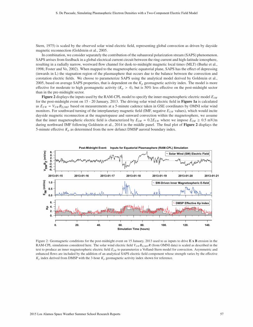
Stern, 1975) is scaled by the observed solar wind electric field, representing global convection as driven by dayside

magnetic reconnection (Goldstein et al., 2005.

In combination, we consider separately the contribution of the subauroral polarization stream (SAPS) phenomenon.

SAPS arrises from feedback in a global electrical current circuit between the ring current and high-latitude ionosphere,

resulting in a radially narrow, westward flow channel for dusk-to-midnight magnetic local times (MLT) (Burke et al.,

1998; Foster and Vo, 2002). When mapped to the magnetospheric equatorial plane, SAPS has the effect of depressing

(inwards in L) the stagnation region of the plasmasphere that occurs due to the balance between the convection and

corotation electric fields. We choose to parameterize SAPS using the analytical model derived by Goldstein et al.,

2005, based on average SAPS properties, that is dependent on the Kp geomagnetic activity index. The model is more

effective for moderate to high geomagnetic activity (Kp > 4), but is 50% less effective on the post-midnight sector

than in the pre-midnight sector.

Figure 2 displays the inputs used by the RAM-CPL model to specify the inner-magnetospheric electric model EIM

for the post-midnight event on 15 - 20 January, 2013. The driving solar wind electric field in Figure 1a is calculated

as ES W = VS W BZ,IMF based on measurements at a 5-minute cadence taken in GSE coordinates by OMNI solar wind

monitors. For southward turning of the interplanetary magnetic field (IMF, negative ES W values), which would incite

dayside magnetic reconnection at the magnetopause and sunward convection within the magnetosphere, we assume

that the inner magnetospheric electric field is characterized by EIM = 0.2ES W where we impose EIM ≥ 0.5 mV/m

during northward IMF following Goldstein et al., 2014 in the middle panel. The final plot of Figure 2 displays the

5-minute effective Kp as determined from the now defunct DMSP auroral boundary index.

Post-Midnight Event: Inputs for Equatorial Plasmasphere (RAM-CPL) Simulation

Solar Wind (SW) Electric Field

SW-Driven Inner Magnetospheric E-field

DMSP Effective Kp Index

2013-01-15 2013-01-16 2013-01-17 2013-01-18 2013-01-19 2013-01-20 2013-01-21

-6.-4.-2.0.2.4.6.

V SWB

Z (mV/

m)

0.0

0.5

1.0

E IM (m

V/m

)

0.2.4.6.

Kp

0. 20. 40. 60. 80. 100. 120. 140.Simulation Time (hours)

Figure 2: Geomagnetic conditions for the post-midnight event on 15 January, 2013 used to as inputs to drive E x B erosion in the

RAM-CPL simulations considered here. The solar wind electric field VS W BZ,IMFR (from OMNI data) is scaled as described in the

text to produce an inner magnetospheric electric field EIM to parameterize a Volland-Stern model for convection. Asymmetric and

enhanced flows are included by the addition of an analytical SAPS electric field component whose strength varies by the effective

Kp index derived from DMSP with the 3-hour Kp geomagnetic activity index shown for reference.



3. Plasmasphere Dynamics on 15-20 January, 2013

Simulated equatorial plasmaspheric densities are produced at the 5-minute cadence of the input parameters shown

in Figure 2. Proceeding from the 15 of January, 2013 onwards over the next few days we see the formation of a

narrowly extended plasmapause suggestive of a plume of plasma whose evolution is expressed in Figure 3. This

geomagnetic event, observed by Van Allen Probes A in the post-midnight magnetic local time sector is moderate in

strength yet still compresses part of the plasmasphere within L = 4 as seen 75 hours into the simulation by the indicated

20 cm−3 low-density threshold plasmapause. We find good agreement with the behavior of the plasmasphere for this

same time interval as that reported for a plasmapause test particle model in Goldstein et al., 2014. This work, however,

expands the previous investigation by also comparing simulated density values of a virtual satellite pass through the

RAM-CPL produced equatorial plasmasphere and the actual density measurements reported by EMFISIS. Figure4 highlights from 12:00 UT on the 15th to 00:00 UT on 18th of January, 2013. RAM-CPL shows less than an

order of magnitude difference fidelity with EMFISIS densities, lending support that it is a useful tool to study the

plasmasphere. Although the actual identified plasmapause locations do not always correspond to steepest density

gradients in the observations or simulations, there is still a close proximity between the two that we will investigate

further in this paper. It is worth noting that regions in which EMFISIS density has been extracted from continuum

radiation at the low-frequency cutoff of the plasma frequency provide only an upper limit to the expected electron

density (Kurth et al., 2015). Thus, the strictly defined low-density (20 cm−3) threshold of the plasmapause located at

21:00 UT on 17 January, 2013 constitute perhaps a misidentification.



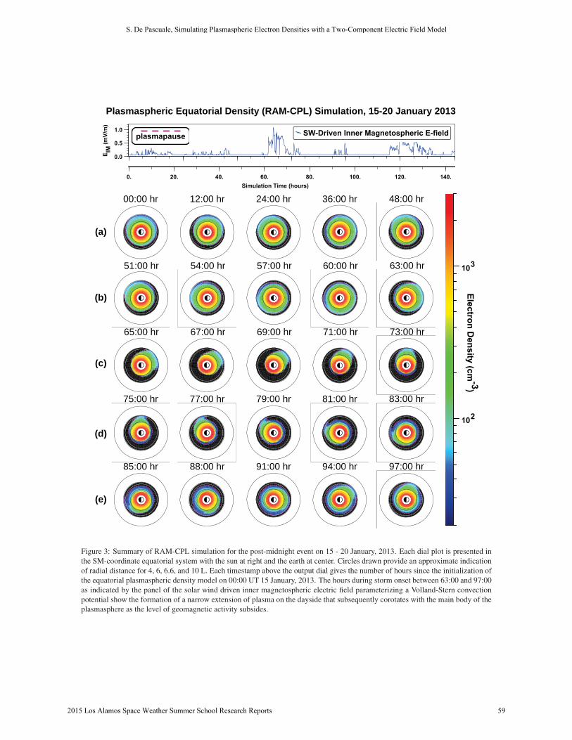
00:00 hr 12:00 hr 24:00 hr 36:00 hr 48:00 hr

51:00 hr 54:00 hr 57:00 hr 60:00 hr 63:00 hr

65:00 hr 67:00 hr 69:00 hr 71:00 hr 73:00 hr

75:00 hr 77:00 hr 79:00 hr 81:00 hr 83:00 hr

85:00 hr 88:00 hr 91:00 hr 94:00 hr 97:00 hr

102

103

Electron Density (cm

-3)


0.0

0.5

1.0

E IM (m

V/m

)

SW-Driven Inner Magnetospheric E-fieldplasmapause

0. 20. 40. 60. 80. 100. 120. 140.Simulation Time (hours)Simulation Time (hours)

(a)

(b)

(c)

(d)

(e)

Plasmaspheric Equatorial Density (RAM-CPL) Simulation, 15-20 January 2013

Figure 3: Summary of RAM-CPL simulation for the post-midnight event on 15 - 20 January, 2013. Each dial plot is presented in

the SM-coordinate equatorial system with the sun at right and the earth at center. Circles drawn provide an approximate indication

of radial distance for 4, 6, 6.6, and 10 L. Each timestamp above the output dial gives the number of hours since the initialization of

the equatorial plasmaspheric density model on 00:00 UT 15 January, 2013. The hours during storm onset between 63:00 and 97:00

as indicated by the panel of the solar wind driven inner magnetospheric electric field parameterizing a Volland-Stern convection

potential show the formation of a narrow extension of plasma on the dayside that subsequently corotates with the main body of the

plasmasphere as the level of geomagnetic activity subsides.



Figure 4: Highlight of EMFISIS RBSP-A in situ density measurements (black) compared to virtual observations (green) through

the equatorial plasmaspheric density model RAM-CPL from 12:00 UT on 15th to 00:00 UT on the 18th of January, 2013. Light

vertical bars correspond to actual plasmapause crossings of the RBSP-A spacecraft as determined by a low-density (20 cm3)

threshold. As described in the text, a region in which continuum radiation was used to identify the upper limit of the local plasma

density is labeled.

4. Determining Plasmapause Encounters

We further investigate the correspondence between actual plasmapause crossings from EMFISIS measurements

and virtual plasmapause crossings from the RAM-CPL simulation. For this post-midnight event on 15 - 20 January,

2013 we find a mean agreement between the model and observations of ΔLAVG = 0.52 ± 0.15RE as shown in Figure5 and Figure 6a. The case in which continuum radiation was used to provide a density measurement does affect

this analysis slightly, but only 1 case out of the 28 total palsmapause crossings had this caveat. Moreover, the model

plasmapause locations only contained 2 false positives, demonstrating the validity of RAM-CPL. When this compar-

ison is expressed in terms of the driving inner magnetospheric electric field conditions we see that the largest range

of errors is correlated with quiet levels of geomagnetic activity at the defined EIM ≥ 0.5 mV/m. The pre-midnight

31 May - 5 June, 2013 event was deliberately excluded from this paper because this effect was more pronounced for

that storm and inhibited a sufficient analysis. But, Figure 6b does imply, at least super superficially, that the spec-

ified level of viscous solar wind interaction with the magnetosphere during northward turning of the interplanetary

magnetic field does regulate to some degree the RAM-CPL modeled extent of the plasmasphere.



Post-Midnight Event: RAM-CPL vs. RBSP A EMFISIS Plasmapause Locations


Actual Plasmapause CrossingsVirtual Plasmapause Crossings

Difference: Model - Observed

2013-01-15 2013-01-16 2013-01-17 2013-01-18 2013-01-19 2013-01-20 2013-01-210.00.20.40.60.81.01.2

E IM (m

V/m

)

3.

4.

5.

6.

7.

L-va

lue

-3.-2.-1.0.1.

L M -

L O

0. 20. 40. 60. 80. 100. 120. 140.Simulation Time (hours)

Delta LAVG = 0.52

Figure 5: Simulated plasmapause locations from RAM-CPL vs RBSP-A EMFISIS density identifications on 15 - 20 January, 2013.

The inner magnetospheric electric field (top panel) controls the extent of the plasmasphere in these simulations and also, to some

degree, corresponds to the geomagnetic activity level affecting the actual plasmasphere. Both the actual crossings (black line) and

virtual crossings (magenta line) show the relationship between inward plasmapause movement and convection (increased EIM).

The mean difference between both actual and virtual detections is ΔLAVG = 0.52 ± 0.15RE as presented in the bottom panel.

3.5 4.0 4.5 5.0 5.5 6.0 6.5 7.0LRBSP-A

3.5

4.0

4.5

5.0

5.5

6.0

6.5

7.0

L RA

M-C

PL

0.0 0.2 0.4 0.6EIM (mV/m)

-4.

-3.

-2.

-1.

0.

1.

2.

Del

ta L

-val

ue

(a) Model vs. RBSP A (b) Difference vs. E-field

Figure 6: Simulated plasmapause locations versus actual plasmapause locations on 15 - 20 January, 2013 with respect to their

correspondence (a) and correlation (b) with the driving inner magnetospheric electric field, EIM . Greater disagreement was found

during quieter conditions.



5. Summary and Conclusions

This paper demonstrates the applicability of a two-component electric field model driving convective erosion in the

plasmasphere during 15 - 20 January, 2013. A combined Volland-Stern and SAPS electric potential, driven separately

by the solar wind and Kp index respectively, produced favorable agreement between the equatorial plasmaspheric

density simulations and RBSP-A EMFISIS observations. The virtual satellite pass encountered electron densities

within an order of magnitude of RBSP-A measurements and all 28 plasmapause crossings during the post-midnight

event with only 2 false positives. This reliability is further bolstered by valid identification of the plasmapause, as

defined by a low-density threshold of 20 cm−3, for a mean model-observation difference of ΔLAVG = 0.52 ± 0.15RE .

It is suggested that the noted correlation between greater disagreement and quieter geomagnetic conditions should be

further inspected with other case studies. A detailed comparison with the pre-midnight 31 May - 5 June, 3013 event

will help to identify this source of error as a physical or analytical consequence.

References

Bilitza, D. (1986). International Reference Ionosphere: recent developments. Radio Sci 21, 343, 1986.

Borovsky, J.E., D.T Welling, M.F. Thomsen, M.H. Denton (2014). Long-lived plasmaspheric drainage plumes: Where does the plasma come from?

J Geophys Res 119, 6496-6520.

Burke, W.J., et al. (1998). Electrodynamics of the inner magnetosphere observed in the dusk sector by CRRES and DMSP during the magnetic

storm of June 4-6, 1991. J of Geophys Res 105, 18, 391.

Carpenter, D.L. (1963). Whistler evidence of a ”Knee” in the magnetospheric ionization density profile. J of Geophys Res 68, 1675 - 1682.

Carpenter, D.L. and Anderson, R.R. (1992). An ISEE/Whistler model of equatorial electron density in the magnetosphere. J of Geophys Res 97,

A2, 1097-1108.

Carpenter, D.L. and Lemaire, J. (1997) Erosion and recovery of the plasmasphere in the plasmapause region. Space Sci Rev 80, 153-179.

Chappell, Cr., Harris, K.K., Sharp, G.W. (1970). The morphology of the bulge region of the plasmasphere. J of Geophys Res 75, 19, 3848-3861.

Chen, A.J., and Wolf, R.A. (1971). Effects on the plasmasphere of a time-varying convection electric field. Planet Space Sci 20, 483-509.

Darrouzet, F. et al. (2009). Plasmaspheric density structures and dynamics: Properties observed by the CLUSTER and IMAGE missions. Space

Sci Rev 14, 55-106.

Foster, J.C., and Burke, W.J. (2002). SAPS: A new categorization for sub-auroral electric fields, Eos Trans AGU 83, 36, 393.

Foster, J.C., and Vo, H.B. (2002). Average characteristics and activity dependence of the sub auroral polarization stream. J of Geophys Res 107.

A12), 1475.

Fok, M.C., Kozyra, J.U., Nagy, A.F., Cravens, T.E. (1991). Lifetime of ring current particles due to Coulomb collisions in the plasmasphere. J of

Geophys Res 96, 7861-7867.

Ganguli, G., Reynold, M.A., Liemohn, M.W., 2000. The plasmasphere and advances in plasmaspheric research. J of Atmos and Solar-Terrestrial

Physics 62, 1647-1657.

Goldstein, J. Burch, J.L., and Sandel, B.R. (2005). Magnetospheric model of sub auroral polarization stream. J of Geophys Res 110, A09222.

Goldstein, J., De Pascuale, S., Kletzing, C., Kurth, W., Genestreti, K.J., Skoug, R.M., Larsen, B.A., Kistler, L.M., Mouikis, C., Spence, H. (2014).

Simulation of Van Allen Probes plasmapause encounters. J of Geophys Res, doi:10.1029/2014JA020252, in press.

Gordon, C.W., Canuto, V., and Axford, W.I. (1978). The Earth, 1: The Upper Atmosphere, Ionosphere, and Magnetosphere. Gordon and Breach

Science Publishers. 40.

Hedin, A.E. (1987). MSIS-86 thermospheric model. J Geophys Res 92, 4649.

Jordanova, V.K., Kistler, L.M., Kozyra, J.U., Khazanov, G.V., Nagy, A.F. (1996). Collisional losses of ring current ions. J of Geophys Res 101,

A1, 111-126.

Jordanova, V.K. and Miyoshi, Y. (2005). Relativistic model of ring current and radiation belt ions and electrons: initial results. Geophys Res Lett

32.

Jordanova, V.K., Miyoshi, Y.S., Zaharia, S., Thomsen, M.F., Reeves, G.D., Evans, D.S., Mouikis, C.G., and Fennell, J.F. (2006). Kinetic simula-

tions of ring current evolution during the Geospace Environment Modeling challenge events. J of Geophys Res 111, A11S10.

Jordanova, V.K., Thorn, R.M., Miyoshi, Y. (2010a). Excitation of whistler-mode chorus from global ring current simulations. J Geophys Res 115.

Jordanova, V.K., Zaharia, S., Welling, D.T. (2010b) Comparative study of ring current development using empirical dipolar, and self-consistent

magnetic field simulations. J Geophys Res 115 (2010b).

Kletzing, C.A. et al. (2013). The Electric and Magnetic Field Instrument Suite and Integrated Science (EMFISIS) on RBSP. Space Sci Rev 179,

127-181.



Kurth, W.S. et al. (2015). Electron densities inferred from plasma wave spectra obtained by the Waves instrument on Van Allen Probes. J Geophys

Res 120, 904-914.

Liemohn, M.W., Ridley, A.J., Gallagher, D.L., Ober, D.M., and Kozyra, J.U. (2004). Dependence of plasmaspheric morphology on the electric

field description during the recovery phase of the 17 April 2002 magnetic storm. J Geophys Res 109, A03209.

Liemohn, et al. (2005). Parametric analysis of nightside conductance effects on inner magnetospheric dynamics for the 17 April 2002 storm. J

Geophys Res 110, A12S22.

Liemohn, et al. (2006). Analyzing electric field morphology through data-model comparisons of the GEM Storm Assessment Challenge events. J

Geophys Res 111, A11S11.

Lemaire, J.F., and Gringauz, K.I. (1998). The Earth’s Plasmasphere. Cambridge University Press, New York.

Lyons, L.R., Thorn, R.M., Kennel, C.F. (1972). Pitch-angle diffusion of radiation belt electrons within the plasmasphere. J Geophys Res 77, 19,

3455.

Maynard, N.C., and Chen, A.J. (1975). Isolated cold plasma regions: Observations and their relation to possible production mechanisms. J of

Geophys Res 80, 1009.

Moldwin, M.B. et al. (2002). A new model of the location of the plasmapause: CRRES results. J Geophys Res 107, A11, 1339-1348.

Nishida, A. (1966). Formation of plasmapause by the combined action of magnetospheric convection and plasma escape from the tail. J of Geophys

Res 71, 23, 5669-5679.

Ni, B., et al. (2013). Resonant scattering and resultant pitch angle evolution of relativistic electrons by plasmaspheric hiss. J Geophys Res 118,

7740-7751.

Ober, D.M., et al. (1997). Formation of density troughs embedded in the outer plasmasphere by sub auroral ion drift events. J Geophys Res 102,

A7, 14595-14602.

O’Brien, T.P. and Moldwin, M.B. (2003). Empirical plasmapause models from magnetic indices. Geophys Res Letters 30, 4, 1152-1156

Rasmussen, C.E., Guiter, S.M., and Thomas, S.G. (1993) A two-dimensional model of the plasmasphere: refilling time constants. Planet Space Sci

41, 1, 35-43.

Richards, P.G., and Torr, D.G. (1985). Seasonal, Diurnal, and Solar Cyclical Variations of the Limiting H+ Flux in the Earth’s Topside Ionosphere.

J of Geopphys Res 90, A6, 5216-5268

Singh, A.K., Singh, R.P., Siingh, D. (2011). State studies of Earth’s plasmasphere: A review. Planet Space Sci 59, 810-834.

Stern, D.P. (1975). The motion of a proton in the equatorial magnetosphere. J of Geophys Res 80, 595.

Thaller, S.A. et al. (2015). Van Allen Probes investigation of the large-scale dusk ward electric field and its role in ring current formation and

plasmasphere erosion in the 1 June 2013 storm. J of Geophys Res 120, 4531-4543.

Thorne, R.M. et al. (2013). Rapid local acceleration of relativistic radiation-belt electrons by magnetospheric chorus. Nature 504, 411-414.

Volland, H. (1973). A semi empirical model of large-scale magnetospheric electric fields. J of Geophys Res 78, 171.

Walsh, B.M., et al. (2014). Simultaneous ground- and space-based observations of the plasmaspheric plume and reconnection. Science 343, 6175,

1122-1125.

Weimer, D.R. (2005). Improved ionospheric electrodynamic models and application to calculating Joule heating rates. J of Geophys Res 110,

A05306.

Wygant, J.R., et al. (2013). The Electric Field and Waves Instruments on the Radiation Belt Storm Probes Mission. Space Sci Rev 179, 183-220.



Ion and Electron Heating by Whistler Turbulence: Parametric Studies via Particle-In-Cell Simulation

R. Scott Hughes University of Southern California, Los Angeles, CA 90089

S. Peter Gary Space Science Institute, Boulder, CO 80301

Joseph Wang University of Southern California, Los Angeles, CA 90089

Abstract Wave-particle interactions are studied in a 3D Particle-In-Cell (PIC) model of a homogeneous, collisionless magnetized plasma subjected to an initially narrowband isotropic spectrum of relatively long wavelength whistler fluctuations. A series of simulations is carried out in order to determine the manner in which the heating rate of each population scales with initial fluctuating magnetic energy density εo. In each simulation the plasma β is held fixed at β e=β i= 0.25 within a simulation domain of length Lωpi/c = 5.12, where ωpi denotes the ion plasma frequency, and εo is varied as εo = 0.01, 0.025, 0.05, 0.1, 0.25. As the initial spectrum undergoes a forward cascade to shorter wavelengths with a preference to propagate at highly oblique angles relative to the background magnetic field, the fluctuations resonate with both the electron and ion populations resulting in heating of each respective species. While the electrons are heated primarily along the mean magnetic field lines, the ions experience enhanced heating primarily in the perpendicular direction. These temperature anisotropies are amplified for each species with increasing εo. Furthermore, the spectral anisotropy factor of the cascaded magnetic fluctuation energy grows larger with increasing initial amplitude signifying an increasing preference for propagation across the background magnetic field. The primary result of this study is given by the scaling of maximum particle heating rate as a function of εo. It is shown that the electron heating rate maintains a proportional relationship, while the ion heating rate increases according to a power law εo

σ with σ>1. This suggests that ion heating may become the primary mode of whistler turbulence dissipation at sufficiently high fluctuation amplitudes.

Keywords: Solar Wind, Turbulence, Whistler, Heating, Ion Heating

1. Introduction

Solar wind turbulence near 1 AU is observed as large-amplitude, broadband energy spectra of magnetic field fluctuations with a dependence on the observed frequency f of f -5/3 and the inferred wavenumber (by Taylor’s frozen in flow hypothesis [Taylor, 1938]) k -5/3 over more than three orders of magnitude variation [Alexandrova et al., 2013]. This regime, termed the inertial range, is understood as a nonlinear forward cascade of fluctuations from very long wavelength sources down to a spectral break near 0.2 Hz < f < 0.5 Hz which corresponds approximately to either kc/ωpp ~1 or kρp ~1 1 [Chen et al., 2014]. These two wavenumbers, which are equivalent at βp = 2, are characteristic scale-lengths of the proton population in a proton-electron plasma. 1 Here ωpj represents the jth species plasma frequency, ρj represents the jth species thermal gyroradius. j = i, p and e denotes ions, protons and electrons respectively.


At higher frequencies and shorter wavelengths solar wind magnetic spectra are observed to have steeper wavenumber dependences, following a power law ∝ 𝑘𝑘−𝛼𝛼 with α > 2 [Alexandrova et al., 2013], and strong wavevector anisotropies with 𝑘𝑘⊥ >> 𝑘𝑘∥ 2 [Sahraoui et al., 2009, 2010, 2013; Narita et al., 2011]. A number of solar wind observations indicate that turbulent fluctuations in the wavenumber range 1 < kc/ωpp < 10 consist primarily of incompressible kinetic Alfvén waves [Sahraoui et al., 2009, 2010; Salem et al., 2012; Podesta, 2013; Kiyani et al., 2013; Chen et al., 2013; Roberts et al. 2013]. This short-wavelength regime is frequently called the dissipation range under the assumption that the spectral break corresponds to the onset of dissipation as fluctuation wavelengths become shorter. A minority view is that this regime should be called the dispersion range [Stawicki et al., 2001] because the inertial range break approximately corresponds to the onset of dispersion in magnetosonic-whistler waves. However, observational evidence for the presence of magnetosonic-whistler turbulence at such short wavelengths is weaker [Gary and Smith, 2009; Narita et al., 2011; Perschke et al., 2013, 2014]. As the relative roles of dissipation and dispersion are not yet well established in this regime, the name for this domain adopted here is the kinetic range.

At even shorter, electron scales corresponding to kc/ωpe ~1 and kρe ~1, magnetic fluctuation spectra observed in the solar wind show still steeper wavenumber dependences. At and beyond these scales, spectra can be fit with either a power-law dependence with α > 3 [Sahraoui et al., 2009, 2010, 2013] or an even more rapid exponential decrease [Alexandrova et al., 2009, 2012, 2013]. An exponential decay in the power spectrum is what would be expected at dissipation scales if parallels are drawn with neutral fluid turbulence [Frisch, 1995].

Explaining kinetic range plasma turbulence requires understanding not only nonlinear processes which drive the field fluctuation cascade, but also linear dispersion (that is, the wavevector dependence of the fluctuation mode frequency) and both linear and nonlinear dissipation processes at short wavelengths. The quasilinear premise [Klein et al., 2012] states that some properties of magnetized plasma turbulence can be understood by modeling that turbulence as a collection of randomly phased linear waves. Computer simulations provide substantial evidence that this premise is valid at short wavelengths [Saito et al., 2008; Howes et al., 2011; Chang et al. 2013]; assuming its validity, the approach taken here is to use linear theory to supply the initial dispersion properties of whistler range modes, and utilize fully nonlinear particle-in-cell (PIC) simulations to address the fundamentally nonlinear properties of turbulent cascade and dissipation.

2. Background

Recent PIC studies of the forward cascade of whistler turbulence in collisionless, homogeneous, magnetized electron-ion plasmas include 2D PIC studies with B0 in the computational plane [Gary et al., 2008; Saito et al., 2008, 2010; Saito and Gary, 2012] and fully 3D PIC studies [Chang et al., 2011, 2013, 2014, 2015; Gary et al., 2012]. In each of these works an ensemble of relatively long-wavelength, approximately isotropic, relatively narrowband whistler fluctuations are imposed at t=0, and the simulations follow the subsequent temporal evolution of the fluctuating fields and particles. For all parameter values studied, the whistler fluctuations undergo a forward cascade to a broadband turbulent spectrum extending to shorter wavelengths with wavevector anisotropies of the type 𝑘𝑘⊥ >> 𝑘𝑘∥. These studies addressed only electron heating, demonstrating

1. Electron heating is substantially stronger in Te∥ than in Te⊥. 2. If the initial electron temperature is β e = 0.10, the late-time electron heating increases with increasing

initial fluctuating magnetic field energy εo [Gary et al., 2012]. 3. Over 0.10 < βe < 1.0 the late-time heated electrons exhibit bi-Maxwellian-like velocity distributions, but at

βe = 0.01 turbulent heating produces extended tails in the suprathermal parts of the electron velocity distribution [Chang et al., 2013].

4. If the initial fluctuation amplitudes and the initial electron temperature are fixed so that β e is varied due to changes in ωpe/Ωe (here Ωe denotes the electron cyclotron frequency), the total late-time electron heating rate normalized to Ωe increases with increasing β e. Furthermore the late-time electron temperature anisotropy Te∥/Te⊥ decreases with increasing β e [Chang et al., 2013].

More recent studies have begun to address how whistler turbulence may heat ions as well as electrons. Saito and Nariyuki [2014] used 2D PIC simulations with B0 in the simulation plane to show that forward cascading whistler fluctuations could heat ions in directions perpendicular to the background magnetic field. Hughes et al. [2014] carried out 3D PIC simulations at β e = 0.05 with computational domains large enough to accommodate both magnetosonic and whistler fluctuations. This study showed 2 The subscripts ⊥ and ∥ denote directions relative to the background magnetic field B0.

R. S. Hughes, Ion and Electron Heating by Whistler Turbulence: Parametric Studies via Particle-In-Cell Simulation


1. Ion heating is stronger in Ti⊥ than in Ti∥. 2. Increasing the simulation domain size (allowing for larger initial fluctuation wavelengths) yields

reduced electron heating. 3. Increasing the simulation domain size yields enhanced ion heating. 4. The late-time heated ions exhibit bi-Maxwellian-like velocity distributions.

Several different calculations have been used to examine plasma species heating by fluctuations in turbulent collisionless plasmas. Markovskii et al. [2010] and Markovskii and Vasquez [2010] carried out 2D hybrid simulations (PIC ions, fluid electrons) of magnetosonic turbulence in collisionless plasmas with B0 in the simulation plane and β i = 0.02 in a simulation domain of size L∥ωpi/c = L⊥ωpi/c = 30π with minimum wavenumber kc/ωpi ≅ 0.067. The forward cascade developed the same 𝑘𝑘⊥ >> 𝑘𝑘∥ wavevector anisotropy as in the whistler turbulence PIC simulations mentioned above. For runs with initial spectra consisting of fluctuations propagating parallel but not antiparallel to B0 the ion heating is preferentially perpendicular to the background magnetic field. For initially isotropic spectra the ion heating changes to be predominantly in the parallel/antiparallel directions, but for initial spectra which are bidirectional but only quasi-perpendicular to B0 the ion heating reverts to T⊥ > T∥.

Howes [2010] used a cascade model for Alfvénic turbulence to calculate the ratio of ion and electron heating rates, Qi/Qe, using damping rates derived from linear gyrokinetic dispersion theory. For typical solar wind parameters, the heating rates are weak functions of Te/Ti. If β i = βe < 1, only the electrons are Landau-resonant with Alfvén waves, and electron heating dominates; at β i = β e ≅ 3 the two heating rates are approximately equal, and as β further increases, ions become Landau resonant and that species gains the stronger heating. Wu et al. [2013] used forward cascading Alfvénic turbulence in a 2D PIC model with B0 oblique to the simulation plane in a β i = βe = 0.1 plasma to show that at relatively weak turbulence amplitudes the electrons are preferentially heated, whereas at larger amplitudes ion heating becomes more important.

The intention of the work presented here is to add to the findings of Hughes et al. [2014] by studying the relative rates of ion and electron heating in a collisionless magnetized plasma subjected to whistler turbulence through the use of large-scale three-dimensional PIC simulations. The focus of this study is to characterize the heating rate of each species as a function of the initial magnetic fluctuation amplitude while the system is constrained to an initial β appropriate to typical solar wind conditions near 1 AU.

3. Methodology

3.1. Simulations The present study is carried out using a three-dimensional electromagnetic particle-in-cell code 3D-EMPIC, as

described in Wang et al. [1995] which has been further modified to run at high parallel efficiency on distributed memory architectures. By this algorithm, ions and electrons are treated as individual entities and their six-dimensional phase space trajectories are tracked through the self consistent solution to Maxwell’s equations along with Newton’s equation of motion. The initial conditions consist of a uniform background magnetic field and each particle species is loaded into the domain with a homogeneous spatial distribution and a Maxwellian velocity distribution. Electromagnetic fluctuations having properties consistent with those of whistler modes are then loaded into the domain. The component relative magnitudes of these modes are derived from the numerical solution to the electromagnetic kinetic linear dispersion relation [Gary, 1993]. In total, 150 normal mode fluctuations possessing relatively long wavelengths and random phases are loaded into the domain at various directions of propagation. These modes form an initially long wavelength isotropic wavevector spectrum.

In order to improve the consistency between the initial electromagnetic fluctuations and the initial phase space configuration of the particles, each particle distribution is formed from the superposition of a thermal Maxwellian distribution and a perturbation velocity distribution associated with the field fluctuations. The latter distribution obtains by perturbing the velocity components of each individual particle according to the fluctuating field magnitudes at the location of that particle. The perturbation velocity component amplitudes for each whistler mode for each species are derived from the numerical solution to the electromagnetic kinetic linear dispersion relation, and the phases are calculated via phase relations with the fluctuating electric fields.

The simulations described here consist of a three dimensional Cartesian domain of shape Lx = Ly = Lz = L with length L = 102.4 c/ωpe = 5.12 c/ωpi. The cell spacing is equal to the Debye length, λD, leading to a total of 10243 cells. The electron thermal velocity is set as vte/c = 0.1 and initially Te = Ti. The mass ratio was chosen as mi/me = 400 in order to accelerate the ion dynamics and reduce the required simulation run time. Here it is assumed that qualitatively the physics is unaffected by this choice of mass ratio as long as mi >> me. In Hughes et al. [2014] the plasma β was set at β e = 0.05. This value is relatively low for realistic conditions in the solar wind near 1 AU



(typically β ~ 1) but allowed for a very clear depiction of ion heating. The current simulations move toward more realistic conditions with a value β e = 0.25. The single parameter allowed to vary in this study was the initial dimensionless magnetic fluctuation energy density, defined as

𝜀𝜀0 = ∑ 𝛿𝛿|𝑩𝑩𝐤𝐤|2/𝐵𝐵02𝐤𝐤 (1) where δ|Bk| is the magnetic fluctuation amplitude of the mode with wavevector k (each initial mode is given equal amplitude) and B0 is the background magnetic field strength. Five simulations were run with values εo = 0.01, 0.025, 0.05, 0.1, 0.25. A point was made to chose values which satisfy the condition εo ≤ β as in the solar wind the thermal pressure is typically greater than the fluctuation energy density on kinetic scales.

3.2. Numerical Validation The particle-in-cell algorithm can introduce nonphysical heating, in part resulting from the use of a discretized

mesh but also due to a limited number of particles per cell. Due to computational memory constraints 32 super-particles of each species (i.e. 32 ions, 32 electrons) per cell were used in this study. In order to quantify the effects of this choice of particle count and the ensuing ”thermal” noise, a run was carried out with no initial fluctuations in the system. All other parameters are the same as those described above. Under these conditions the simulated plasma should remain in an equilibrium condition and no heating should occur. Figure 1 displays the energy density profiles with time for this test run. While zero energy exchange is not achieved the effect of the numerical techniques employed is actually to slightly and gradually cool the particles. The ion cooling is proportional to the electron cooling by the square root of their mass ratio. The source of this cooling can be attributed to the use of a Gaussian filter which is applied to the calculated current density at each time step in order to counteract numerical heating. Figure 1 reveals that the Gaussian filter over-corrects, and the particles are slightly cooled. In any event, the level to which the particles are cooled is, in most cases, well below that of the level to which they are heated when initial fluctuations are present. For example, in comparing with the case of ε0 = 0.05 from figure 3, the electrons are heated to 10 times that by which they are cooled in this test case. Thus, such effects are justifiably neglected in the following results.

Figure 1: Results of a run with no initial fluctuation energy, quantifying the numerical effects on particle heating. The electromagnetic (red),

electron (green) and ion (black) energy densities normalized by the background magnetic field energy density are shown.

3.3. Diagnostics The primary plasma property under investigation here is the temperature of each species, along with the rate of

change in temperature. Previous studies (e.g. Hughes et al., 2014) calculated this property by finding the variance in velocity of each species over the entire domain. This provided a calculation of thermal velocity from which the temperature in each direction can be obtained according to kBTj = mjvtj

2. Calculating the temperature in this way resulted in rapid ion heating followed by large oscillations in the ion temperature time history (see figure 2). The problem was that the measured value was composed of two components: the energy associated with irreversible heating of the population, i.e. the temperature, along with a component attributed to reversible oscillatory motions induced through interactions with the field fluctuations. The latter component is associated with spatial structure and should not be accounted for in the calculation of temperature.

To this end, an improved temperature diagnostic was developed for this investigation. The approach to removing the fluctuation component was to calculate the temperature at each individual cell, rather than throughout the entire domain, then to remove any oscillatory structures in the calculated temperature field. From a Fourier-space perspective this is synonymous with keeping only the k = 0 mode of the temperature wavevector spectrum, which can be calculated more simply as the average temperature across all cells. The improved temperature diagnostic is therefore given as



𝑘𝑘𝐵𝐵𝑇𝑇𝑗𝑗 =1

𝑁𝑁𝑥𝑥𝑁𝑁𝑦𝑦𝑁𝑁𝑧𝑧

12𝑚𝑚𝑗𝑗[< 𝑣𝑣2 >𝑗𝑗𝑗𝑗 −< 𝑣𝑣 >𝑗𝑗𝑗𝑗

2 ]

𝑁𝑁𝑥𝑥𝑁𝑁𝑦𝑦𝑁𝑁𝑧𝑧

𝑗𝑗=1

(2)

Where l is the scan-line coordinate of each cell and j denotes the species. This calculation is carried out for each velocity vector component to obtain a temperature in each orthogonal direction.

As previous work was performed according to a less than ideal method for calculating the temperature, it is appropriate to perform a comparison study in order to understand the consequences in this change in diagnostics. Figure 2 shows the results of this study. The parameters used in this comparison are those as used in Hughes et al. [2014], namely β e = 0.05, εo = 0.1 in a three dimensional domain of size L = 51.2 c/ωpe. Panel (a) of figure 2 shows that there is little difference in diagnostic method for the electrons. The new diagnostic differs from the old at the beginning of the simulation, where the new diagnostic reveals the electron’s attempt to become self consistent with the initial spectrum of fluctuations. Shortly after time t=0, both diagnostics agree well. A much more obvious difference is revealed in panel (b) for the ion population. The temperature profiles are more gradual and smooth under the new diagnostic. The most important feature of figure 2 is that, in the asymptotic limit, both diagnostics agree well, that is, the solutions converge at late simulation times. The new diagnostic is far better suited to studying heating rates as the ion temperature profiles appear to behave more appropriately. However, results from Hughes et al. 2014 remain valid, as heating rates weren’t investigated, rather the important feature there was the total (late time) heating, which converges under the previously used temperature diagnostic.

Figure 2: Comparison of the previously used temperature diagnostic with the improved (new) temperature diagnostic. (a) Electron temperatures (b) ion temperatures normalized by initial temperature. Parallel and perpendicular temperatures are shown.

4. Results

Following the simulation set up described in section 3.1, the results of this study are now presented. Figure 3 shows properties of the fluctuating fields as a function of time at each initial value of εo. Panel (a) illustrates that in each case the fields undergo and exponential-like decay of energy as the plasma constituents resonate with the fluctuations. The fraction of initial fluctuation energy transferred to the particles increases monotonically with increasing initial amplitude. The fluctuation half-life can be fitted to the power law

𝑡𝑡1/2 = 528𝜀𝜀0−0.34 (3) with R2 = 0.95. Panel (b) shows the spectral anisotropy factor over the duration of each run. The spectral anisotropy factor is defined as [Gary et al. 2012]

tan2(θ𝐵𝐵) =∑ 𝑘𝑘⊥2𝒌𝒌 |𝛿𝛿𝑩𝑩(𝑘𝑘⊥,𝑘𝑘∥)|2

∑ 𝑘𝑘∥2𝒌𝒌 |𝛿𝛿𝑩𝑩(𝑘𝑘⊥, 𝑘𝑘∥)|2 (4)

and describes the preferential angle of propagation relative to the background magnetic field. Values greater than 1 correspond to a preferential angle greater than 45° and signify a highly oblique spectrum, that is a spectrum satisfying 𝑘𝑘⊥ >> 𝑘𝑘∥. The results of panel (b) are calculated over the region of wavevector space which excludes the initial fluctuations so as to observe the behavior of the fluctuations generated through the forward cascade process. In all runs the spectrum evolves into a perpendicularly anisotropic state. Early simulation times show a rapid increase of this factor as fluctuation energy flows from the initial spectrum into previously empty regions of wavevector space and establishes the forward cascade. After tωpe ~ 650 the behavior becomes approximately linear, with the lowest values of εo maintaining their degree of anisotropy. The three highest values of εo continue to grow



more anisotropic with time, with a higher rate of growth at larger initial fluctuation amplitude. This behavior is interpreted as follows: at early times fluctuation energy cascades to shorter wavelengths, primarily in the perpendicular direction, at a high rate. After the initial fluctuations have transferred energy to sufficiently short wavelengths, dissipation begins to play a prominent role and acts to prevent the spectrum from becoming more anisotropic by removing energy from the quasi-perpendicular, short wavelength region of the spectrum. However, as εo increases more energy is available to continue to drive the quasi-perpendicular cascade and the transfer rate remains larger than the dissipation rate for a longer period of time, allowing the spectrum to grow more anisotropic.

Figure 3: Temporal evolution of field quantities at β = 0.25 and various values of εo as labeled. (a) Total magnetic plus electric field fluctuation

energy (b) Wavevector anisotropy factor calculated over the cascaded region of wavevector space.

The parallel and perpendicular temperature profiles for each species are shown in figure 4. All four panels give the expected result that the heating rate increases monotonically with increasing εo. The electrons are heated significantly more than the ions and experience greater heating rates at early simulation times, which gradually drop and result in a plateau of the temperature profiles by the end of the simulations. The ion temperature profiles, on the other hand, grow more gradually and steadily maintain nearly linear curves from tωpe ~ 500 through the end of the simulations. While the electrons immediately begin interacting with the fluctuations and provide the primary means by which the forward cascade can proceed, the ions show little interaction until the fluctuation spectrum has had time to become sufficiently anisotropic. Linear theory of whistler modes at quasi-perpendicular propagation _

Figure 4: Temporal evolution of the plasma temperatures, normalized by initial temperature, at β = 0.25 and various values of εo as labeled. (a)

Electron parallel temperature (b) electron perpendicular temperature (c) ion parallel temperature (d) ion perpendicular temperature.



predicts that 0 < |δE∥|2 << |δE⊥|2. This condition, along with the anisotropic character of the fluctuation spectrum, implies that such modes will energize the magnetized electrons in directions parallel to the mean field, while the unmagnetized ions will primarily gain energy perpendicular to B0. This is precisely what is observed, as electrons show preferential parallel temperature gain, while the ions are more greatly heated in perpendicular directions.

The temperature anisotropies are made clearer by figure 5. For both the electron and ion populations, the respective anisotropic character is enhanced as εo is increased. As illustrated in figure 3(b) the fluctuation spectrum becomes more anisotropic with εo. As the modes responsible for preferential parallel heating of the electrons and perpendicular heating of the ions propagate at quasi-perpendicular directions, the more anisotropic spectrum implies an increase in the temperature anisotropy. In comparing figures 3(b), 4(a) and 5(a) at times between tωpe = 0 – 200, the early time decrease in electron parallel temperature, and associated increase in the anisotropy factor appears to be associated with the establishment of the anisotropic cascaded spectrum. While the initial isotropic fluctuations heat electrons in the perpendicular direction, interactions in the parallel direction drive fluctuation energy toward shorter perpendicular wavelengths rather than toward higher parallel electron temperatures. Once these quasi-perpendicular fluctuations are established, the primary mode of dissipation is through parallel heating of the electrons, and the temperature anisotropy rapidly drops below 1.

Figure 5: Plasma temperature anisotropy factors with time. (a) Electron T⊥/T∥ (b) ion T⊥/T∥.

The maximum heating rate of each plasma population as a function of initial fluctuation amplitude is illustrated in figure 6. That is, the maximum value of energy gain at any time after tωpe = 200, when the cascaded spectrum has become established, is determined from the calculated heating rate profiles (not shown) and plotted for each simulation. The dimensionless time rate of energy gain of species j is defined as Qj = [dTj/dt]/[Tj (t=0)ωpj]. The dotted and dashed lines provide linear profiles which aren’t fit to the data, but rather allow for visual comparison with the trends in the data. The electron data points agree well with the dotted line, maintaining a linear _

Figure 6: The maximum values of the dimensionless time rates of change of the perpendicular ion temperature (red dots), the parallel ion temperature (red squares), the total ion temperature (orange diamonds), and the total electron temperature (blue diamonds) as functions of

εo at β = 0.25. The dashed lines represent the equations Qi = 0.00015εo and Qe = 0.002εo drawn to guide the eye.



progression over the range of values of εo. The ion heating trend is rather different. At very low values of εo the trend is nearly linear. However, for εo = 0.05 – 0.25 the values increase at a rate greater than linear, scaling as εo

σ with σ > 1. As the fluctuation amplitudes become larger the ion heating rates approach those of the electron heating rates. This suggests that at sufficiently large amplitude, ion heating may become the primary mode of dissipation.

An important simulation result here is that both species heating rates scale with fluctuating field energy density at small values of εo, consistent with predictions of quasilinear-like second order perturbation theories [Gary and Feldman, 1978]. This suggests that quasilinear-like heating rate calculations such as those of Howes [2010] are likely to be valid for sufficiently weak magnetic field fluctuations. The second important result is that the late-time ion heating rates increase as εo

σ with σ > 1 for sufficiently large εo. This transition to an apparently nonlinear ion heating rate is consistent with the results of Wu et al. [2013] who used two-dimensional PIC simulations in much larger simulation domains to show that at sufficiently large amplitudes of Alfvénic turbulence ion heating dominates electron heating.

5. Conclusions

Three-dimensional particle-in-cell simulations were carried out to examine the temporal evolution of initially narrowband spectra of whistler fluctuations in homogeneous, collisionless plasmas with initial β e = 0.25. The fluctuations undergo a forward cascade to shorter wavelengths, developing a broadband, anisotropic spectrum of turbulence which dissipates energy on both electrons and ions. The simulations confirm earlier results for whistler turbulence that electrons gain energy primarily in the direction parallel/antiparallel to the background magnetic field, but that ions are heated primarily in directions perpendicular to B0. Several simulations at different initial fluctuation energy densities were carried out; the computations show that both the perpendicular ion heating rate and the total electron heating rate scale approximately as εo at εo << 1. The computations further demonstrate that the perpendicular ion heating rate increases more rapidly than εo for sufficiently large values of εo.

Whistler fluctuations are of high frequency compared to the proton cyclotron frequency, so that one expects, and our simulations show, that ion heating by whistler turbulence is relatively weak compared to the heating of electrons. However, our results also show that ion turbulent heating appears as preferential energy gain in directions perpendicular to the background magnetic field. Solar corona and solar wind observations show a strong preference for perpendicular ion heating [Cranmer, 2014, and references therein], but at present there is no consensus as to the source of this energy gain. One possible source of such heating is resonant Alfvén-cyclotron waves with kc/ωpi ~1 [Gary and Saito, 2003; Hollweg and Isenberg, 2002; Cranmer, 2014]; another potential source is “stochastic heating” by nonresonant MHD fluctuations [Chandran, 2010], and a third plausible source is resonant magnetosonic-whistler waves [Markovskii et al, 2010; Markovskii and Vasquez, 2010]. Although relatively weak compared to electron heating, the perpendicular heating of the ions demonstrated in these simulations is consistent with the hypothesis that the obliquely propagating component of magnetosonic-whistler turbulence contributes to the persistent perpendicular heating of protons observed in the solar wind. As Hughes et al. [2014] has shown that the efficacy of ion perpendicular heating by whistler fluctuations substantially increases with increasing simulation domain size, it is important that further PIC simulations of magnetosonic-whistler turbulence be carried out at larger computational systems than those used here in order to quantify ion heating rates for comparison against competing candidates for ion energization in the solar wind.

References

Alexandrova, O., J. Saur, C. Lacombe, A. Mangeney, J. Mitchell, S. J. Schwartz, and P. Robert (2009), Universality of solar-wind turbulent spectrum from MHD to electron scales, Phys. Rev. Lett., 103, 165003.

Alexandrova, O., C. Lacombe, A. Mangeney, R. Grappin, and M. Maksimovic (2012), Solar wind turbulent spectrum at plasma kinetic scales, Ap. J., 760, 121.

Alexandrova, O., C. H. K. Chen, L. Sorriso-Valvo, T. S. Horbury, and S. D. Bale (2013), Solar wind turbulence and the role of ion instabilities, Space Sci. Rev., 178, 101.

Chandran, B. D. G. (2010), Alfven-wave turbulence and perpendicular ion temperatures in coronal holes, Ap. J., 7820, 548. Chang, O., S. P. Gary, and J. Wang (2011), Whistler turbulence forward cascade: Three- dimensional particle-in-cell simulations, Geophys. Res.

Lett., 38, L22102. Chang, O., S. P. Gary, and J. Wang (2013), Whistler turbulence and variable electron beta: Three-dimensional particle-in-cell simulations, J.

Geophys. Res., 118, 2824. Chang, O., S. P. Gary, and J. Wang (2014), Energy dissipation by whistler turbulence: Three-dimensional particle-in-cell simulations, Phys.

Plasmas, 21, 052305.



Chang, O., S. P. Gary, and J. Wang (2015), Whistler turbulence forward cascade versus inverse cascade: Three-dimensional particle-in-cell simulations, Ap. J., 800, 87.

Chen, C. H. K., S. Boldyrev, Q. Xia, and J. C. Perez (2013), Nature of subproton scale turbulence in the solar wind, Phys. Rev. Lett., 110, 225002.

Chen, C. H. K., L. Leung, S. Boldyrev, B. A. Maruca, and S. D. Bale (2014), Ion-scale spectral break of solar wind turbulence at high and low beta, Geophys. Res. Lett., 41, 8081.

Cranmer, S. (2014), Ensemble simulations of proton heating in the solar wind via turbulence and ion cyclotron resonance, Ap. J. Supplement Series, 213, 16.

Frisch, U. (1995), Turbulence: The Legacy of A. N. Kolmogorov, Cambridge University Press, Cambridge. Gary, S. P. and W. C. Feldman (1978), A second-order theory for k || B0 electromagnetic instabilities, Phys. Fluids, 21, 72. Gary, S. P. (1993), Theory of space plasma microinstabilities, Cambridge University Press, New York. Gary, S. P., and S. Saito (2003), Particle-in-cell simulations of Alfven-cyclotron wave scattering: Proton velocity distributions, J. Geophys. Res.,

108, 1194. Gary, S. P., S. Saito, and H. Li (2008), Cascade of whistler turbulence: Particle-in-cell simulations, Geophys. Res. Lett., 35, L02104. Gary, S. P., and C. W. Smith (2009), Short-wavelength turbulence in the solar wind: Linear theory of whistler and kinetic Alfven fluctuations, J.

Geophys. Res., 114, A12105. Gary, S. P., O. Chang, and J. Wang (2012), Forward cascade of whistler turbulence: Three-dimensional particle-in-cell simulations, Ap. J., 755,

142. Hollweg, J., and P. Isenberg (2002), Generation of the fast solar wind: A review with emphasis on the resonant cyclotron interaction, J. Geophys.

Res., 107(A7), 1147. Howes, G. G. (2010), A prescription for the turbulent heating of astrophysical plasmas, Mon. Not. R. Astron. Soc, 409, L104. Howes, G. G., J. M. TenBarge, W. Dorland, E. Quataert, A. A. Schekochihin, R. Numata, and T. Tatsuno (2011), Gyrokinetic simulations of

solar wind turbulence from ion to electron scales, Phys. Rev. Lett., 107, 035004. Hughes, R. S., S. P. Gary, and J. Wang (2014), Electron and ion heating by whistler turbulence: Three-dimensional particle-in-cell simulations,

Geophys. Res. Lett., 41, 8681. Kiyani, K. H., S. C. Chapman, F. Sahraoui, B. Hnat, O. Fauvarque, and Yu. V. Khotyaintsev (2013), Enhanced magnetic compressibility and

isotropic scale- invariance at sub-ion Larmor scales in solar wind turbulence, Ap. J., 763, 10. Klein, K. G., G. G. Howes, J. M. TenBarge, S. D. Bale, C. H. K. Chen, and C. S. Salem (2012), Using synthetic spacecraft data to interpret

compressible fluctuations in solar wind turbulence, Ap. J., 755, 159. Markovskii, S. A., and B. J. Vasquez (2010), The effect of spectral anisotropy of fast magnetosonic turbulence on the plasma heating at the

proton kinetic scales, Phys. Plasmas, 17, 112902. Markovskii, S. A., B. J. Vasquez, and B. D. G. Chandran (2010), Perpendicular proton heating due to energy cascade of fast magnetosonic waves

in the solar corona, Ap. J., 709, 1003. Narita, Y., S. P. Gary, S. Saito, K.-H. Glassmeier, and U. Motschmann (2011), Dispersion relation analysis of solar wind turbulence, Geophys.

Res. Lett., 38, L05101. Perschke, C., Y. Narita, S. P. Gary, U. Motschmann, and K.-H. Glassmeier (2013), Dispersion relation analysis of turbulent magnetic field

fluctuations in fast solar wind, Ann. Geophys., 31, 1949. Perschke, C., Y. Narita, U. Motschmann, and K.-H. Glassmeier (2014), Multi-spacecraft observations of linear modes and sideband waves in ion-

scale solar wind turbulence, Ap. J. Lett., 793, L25. Podesta, J. J. (2013), Evidence of kinetic Alfven waves in the solar wind at 1 AU, Solar Phys., 286, 529. Roberts, O. W., X. Li, and B. Li (2013), Kinetic plasma turbulence in the fast solar wind measured by Cluster, Ap. J., 769, 58. Sahraoui, F., M L. Goldstein, P. Robert, and Yu. V. Khotyaintsev (2009), Evidence of a cascade and dissipation of solar-wind turbulence at the

electron gyroscale, Phys. Rev. Lett., 102, 231102. Sahraoui, F., M L. Goldstein, G. Belmont, P. Canu, and L. Rezeau (2010), Three dimensional anisotropic k spectra of turbulence at subproton

scales in the solar wind, Phys. Rev. Lett., 105, 131101. Sahraoui, F., S. Y. Huang, G. Belmont, M. L. Goldstein, A. Retino, P. Robert, and J. DePatoul (2013), Scaling of the electron dissipation range of

solar wind turbulence, Ap. J., 777, 15. Saito, S., S. P. Gary, H. Li, and Y. Narita (2008), Whistler turbulence: Particle-in-cell simulations, Phys. Plasmas, 15, 102305. Saito, S., S. P. Gary, and Y. Narita (2010), Wavenumber spectrum of whistler turbulence: Particle-in-cell simulation, Phys. Plasmas, 17, 122316. Saito, S., and S. P. Gary (2012), Beta dependence of electron heating in decaying whistler turbulence: Particle-in-cell simulations, Phys. Plasmas,

19, 012312. Saito, S., and Y. Nariyuki (2014), Perpendicular ion acceleration in whistler turbulence, Phys. Plasmas, 21, 042303. Salem, C. S., G. G. Howes, D. Sundkvist, S. D. Bale, C. C. Chaston, C. H. K. Chen, and F. S. Mozer (2012), Identification of kinetic Alfvén

wave turbulence in the solar wind, Ap. J., 745, L9. Stawicki, O., S. P. Gary, and H. Li (2001), Solar wind magnetic fluctuation spectra, J. Geophys. Res., 106, 8273. Taylor, G. I. (1938), The spectrum of turbulence, Proc. R. Soc. Lond. A, 164, 476. Wang, J., P. Liewer, and V. Decyk (1995), 3D electromagnetic plasma particle simulations on a MIMD parallel computer, Comput. Phys.

Commun., 69, 306. Wu, P., M. Wan, W. Matthaeus, M. Shay, and M. Swisdak (2013), von Karman energy decay and heating of protons and electrons in a kinetic

turbulent plasma. Phys. Rev. Lett., 111(12), 121105.



The statistics of relativistic electron pitch angle distribution in the Earth’s radiation belt based on the Van Allen Probes measurements

Hong Zhao Laboratory for Atmospheric and Space Physics and Department of Aerospace Engineering Sciences, University of Colorado at Boulder, Boulder,

CO 80302

Reiner Friedel Los Alamos National Laboratory, Los Alamos, NM 87545

Abstract The relativistic electron pitch angle distribution (PAD) is an important characteristic of radiation belt electrons, which can give information on source or loss processes in a specific region. Using data from MagEIS and REPT instruments onboard the Van Allen Probes and LANL-GEO satellites, a statistical survey of relativistic electron pitch angle distribution (PAD) is performed. By fitting relativistic electron PADs to Legendre polynomials, an empirical model of PADs as a function of L (from 1.4 to 6), MLT, electron energy (~100 keV – 5 MeV), and geomagnetic activity is developed and many intriguing results are found. In the outer radiation belt, an unexpected dawn/dusk asymmetry of ultra-relativistic electrons is found during quiet times, with the asymmetry becoming stronger at higher energies and at higher L shells. This may indicate the existence of physical processes acting on the relativistic electrons on the order of drift period. In the inner belt and slot region, 100s of keV pitch angle distributions with minima at 90° are shown to be persistent in the inner belt and appears in the slot region during storm times. The model also shows clear energy dependence and L shell dependence of 90°-minimum pitch angle distribution. On the other hand, the head-and-shoulder pitch angle distributions are found during quiet times in the slot region, and the energy, L shell and geomagnetic activity dependence of those PADs are consistent with the wave-particle interaction caused by hiss waves.

Keywords: radiation belt electrons, pitch angle distribution, wave-particle interaction

1. Introduction

The relativistic electron pitch angle distribution (PAD) is an important characteristic of radiation belt electrons, which can give valued information on source or loss processes in a specific region. Many previous studies have focused on the characteristics and evolution of electron PADs in the outer radiation belt [e.g., West et al., 1973; Gannon et al., 2007; Chen et al., 2014]. Generally, the electron PADs in the outer radiation belt can be categorized into three types: the normal distribution, butterfly distribution, and flat top distribution. The normal distribution is the most general type of PAD in the outer belt, for which the electron flux peaks at 90° pitch angle (PA) and smoothly decreases at smaller PAs. It is thought to form as a result of the loss to the atmosphere combining with the pitch angle diffusion. Inward radial diffusion can also cause the flux peak around 90°. Due to the conservation of the first and second adiabatic invariant, when an electron moves inward, the perpendicular momentum increases more than the parallel component, which would increase the PA of electron and thus create a more 90° peaked PAD [e.g., Schulz and Lanzerotti, 1974]. The butterfly distribution has a minimum around 90°, which looks like a butterfly in the polar plot (in which PA is the polar angle and flux is the radius). The butterfly distribution is thought to be caused by the drift-shell-splitting effect combining with magnetopause shadowing or strong negative radial flux gradient [e.g., Sibeck et al., 1987; Selesnick and Blake, 2002]. Horne et al. [2005] have also suggested that chorus wave heating could cause butterfly distribution by preferentially heating off-equator electrons. For the flat top


distribution the electron flux is approximately equal at a wide PA range centered around 90°. It can be a transition between the normal distribution and butterfly distribution or can be due to strong wave-particle interactions [Horne et al., 2003]. For tens to hundreds of keV electrons, “cigar” distribution with flux peaking along the direction of local magnetic field has also been found in the outer radiation belt, and it is thought to be related to the tail-like stretching of the nightside magnetic field prior to the substorms and thus could be used as an indicator of likely substorm onset [Baker et al., 1978].

There are also some studies have focused on those in the slot region and inner belt [e.g., Lyons and Williams, 1975a, 1975b; Zhao et al., 2014a, 2014b]. Lyons and Williams [1975a] found “cap” PAD (also called “head-and-shoulder” PAD) in the slot region after electron injections and during geomagnetic quiet times, which looks like a bump around 90° on top of a normal distribution. As for the formation of cap distributions, Lyons and Williams [1975a] shows the comparison between the observation and modeling of wave-particle interaction, and the agreement between the two suggests that the cap distribution forms as a result of pitch angle scattering caused by the plasmaspheric whistler mode waves in the slot region. However, Sibeck et al. [1987] has also found the cap distribution in the outer belt and suggested that this type of PAD in the outer radiation belt can be caused by a combination of the drift-shell-splitting effect and a substorm injection or a sudden magnetospheric compression. Recently, Zhao et al. [2014a] reported a new type of PADs of 100s of keV electrons in the inner belt and slot region using the observation from Van Allen Probes. This PAD type, called “90°-minimum PAD” here, shows as a Gaussian distribution with a small bite out around 90°. It is generally present in the inner belt and occurs in the slot region during storm times. While the wave-particle interaction caused by fast magnetosonic waves is suggested as one possible mechanism, the actual physical processes responsible for the formation of this type of PADs are still under debate.

The electron pitch angle distribution reflects the effects of different physical processes and the competition between them in a specific region. Understanding the evolution of pitch angle distributions can contribute to the identifying and understanding of those processes and thus the understanding of the inner magnetospheric dynamics. In this report, using data from REPT and MagEIS instruments on the Van Allen Probes and LANL GEO satellites, we construct an empirical model of relativistic electron PADs by fitting PADs into Legendre polynomials. Focusing on the MeV electrons in the outer radiation belt and 10s to 100s of keV electrons in the low L region respectively, the averaged PADs as a function of L, MLT, electron energy, and geomagnetic activity are shown and some intriguing results are found.

2. Data

In this study, pitch-angle-resolved electron flux data from REPT [Baker et al., 2013] and MagEIS [Blake et al, 2013] instruments onboard Van Allen Probes are used. The Van Allen Probes, launched on 30 Aug 2012, operate in an elliptical orbit with an inclination of 10° and altitude of ~600 km × 5.8 RE [Kessel et al., 2013]. MagEIS provides high-resolution energetic electron flux measurements with energy range of ~35 – 4000 keV. It contains four independent magnetic electron spectrometers on each spacecraft, one low energy spectrometer (LOW), two medium energy spectrometers (M75 and M35) and a high energy spectrometer (HIGH). The low unit, high unit, and one of the medium units (M75) are mounted with the field of view centered at 75° to the spin axis, while the field of view of another medium unit (M35) is centered at 35° to provide larger PA coverage. REPT provides high-quality measurement of relativistic electrons with energy from ~ 2 MeV to ~20 MeV. However, since the counts for ultra-relativistic electrons are too low to show clear PADs, only data for electrons with energy from 1.8 MeV to 3.6 MeV are used in this study. The MagEIS and REPT data are averaged into 1-min bins and 10° PA bins. For REPT data, to eliminate the influence of background contamination, only PADs with total counts greater than 100 are included. Only those data when Van Allen Probes are near the magnetic equator with magnetic latitude < 10° are used in our study, and the electron PADs are propagated to the magnetic equator using T89D magnetic field model [Tsyganenko, 1989] unless otherwise noted. With the spin axis approximately pointing to the Sun, the spacecraft is spinning with a period of ~12s, which provides good pitch angle coverage during most times and thus provides an ideal data set for pitch angle distribution studies.

Pitch-angle-resolved data from Los Alamos National Laboratory Geosynchronous (LANL-GEO) satellites [Reeves et al., 1997] are also used in this study. The LANL-GEO data are also averaged and binned into 15° PA bins. With measured electron energies up to ~1.5 MeV, LANL-GEO data are used to show the electron PADs at different MLTs at geosynchronous orbit.

H. Zhou, The statistics of relativistic electron pitch angle distribution in the Earth’s radiation belt based on the Van Allen Probes measurements


3. Methodology

To construct a statistical model for relativistic electron PADs, we choose to fit PADs to Legendre polynomials. The electron PADs can be expressed as

𝑗𝑗(𝛼𝛼) = 𝐶𝐶𝑛𝑛𝑃𝑃𝑛𝑛[cos (𝛼𝛼)]∞

𝑛𝑛=0

where 𝑗𝑗(𝛼𝛼) is the flux of electrons with pitch angle α, 𝑃𝑃𝑛𝑛[cos (𝛼𝛼)] is the nth-degree Legendre polynomial, and 𝐶𝐶𝑛𝑛 is the corresponding coefficient. The coefficient of each Legendre polynomial can be calculated using the orthogonal property:

𝐶𝐶𝑛𝑛 =2𝑛𝑛 + 1

2 𝑗𝑗(𝛼𝛼)𝑃𝑃𝑛𝑛[cos(𝛼𝛼)]sin (𝛼𝛼)𝑑𝑑𝛼𝛼𝜋𝜋

0

The coefficients derived using this equation are then normalized as

𝑐𝑐𝑛𝑛 =𝐶𝐶𝑛𝑛𝐶𝐶0

Here 𝐶𝐶0 is the actual directionally averaged flux. Any PAD can be fully represented by a whole set of Legendre polynomials. However, in a statistical model we

can only keep finite number of coefficients and the number of coefficients should be kept as small as possible. Based on the previous study [Chen et al., 2014], 𝐶𝐶𝑛𝑛 decreases quickly with increasing n, and including the Legendre polynomials up to 6th-degree is enough to reproduce most observed PADs in the outer radiation belt. Thus we fit measured PADs in the outer radiation belt to a summation of 0th to 6th degree Legendre polynomials. However, the situation in the inner belt and slot region is very different. The electron PADs in the inner belt and slot region usually have some detailed features, e.g., 90°-minimum PAD and cap PAD, which cannot be well represented by Legendre polynomials up to 6th degree. Thus for PADs in the low L region (L<3.5) we use Legendre polynomials up to 10th degree. In addition, the electron PADs in the radiation belt are expected to be symmetric with respect to 90° pitch angle. In this study, to give a full coverage on all pitch angles, we average PADs measured by Van Allen Probes in bins of 10° PA and force them to be symmetric, and thus the coefficients even-th degree Legendre polynomials are zero.

The accuracy of our model strongly depends on the accuracy of the fitting results, so we use the PADs that can be well represented by the Legendre polynomials to construct the statistical model. Only good fits with root-mean-square-deviation (RMSD)

𝑅𝑅𝑅𝑅𝑅𝑅𝑅𝑅 = ∑ (𝑙𝑙𝑙𝑙𝑙𝑙(𝚥𝚥) − 𝑙𝑙𝑙𝑙𝑙𝑙 (𝑗𝑗))2𝑛𝑛

𝑛𝑛< 0.05

are included in the statistics, where 𝑗𝑗 is the measured flux and 𝚥𝚥 is the fitting results. According to our results, most fits are valid. For example, for REPT E=1.8 MeV electrons, only 10% fits are rejected due to poor fitting. This also validates our fitting method. On the other hand, it is essential to make sure the fitting results represent the real PADs, so only PADs with full PA coverage have been included. PADs with no data points within high PA range [80°, 100°] or low PA range [0°, 20°]/[160°, 180°] are excluded from the statistics.

Based on this fitting method, a statistical relativistic electron equatorial PAD model is constructed as a function of L, MLT, geomagnetic activity and electron energy using data from MagEIS and REPT from Sep 2012 to June 2015. The model includes 26 L bins from L=1 to L=6 with ΔL = 0.2 and 12 MLT bins with ΔMLT = 2. Note that for ~MeV and more energetic electrons our model only includes L shells down to L=3 since in the slot region and inner belt the fluxes of these electrons are usually too low to show clear PAD pattern. The geomagnetic activity, represented by the geomagnetic indices Dst, is divided into three levels. The medians and standard deviations of coefficients are derived and recorded in each L and MLT bin for electrons with a specific energy under a specific geomagnetic condition. The averaged PADs shown in the following section are generated using medians of coefficients at each L shell, MLT, geomagnetic activity level for electrons with a specific energy. The main results are as follows.

4. Results

Using the method described in section 3, we construct a statistical model for electron PADs as a function of L, MLT, geomagnetic activity, and electron energy using data from Van Allen Probes. In this section, we will show the medians of these coefficients and averaged PADs as well as their dependence on L, MLT, geomagnetic activity and



electron energy, mainly focusing on the >MeV electron PADs in the high L region and 10s to 100s of keV electron PADs in the low L region.

4.1. The dawn-dusk asymmetry of ultra-relativistic electron PADs in the high L region Using data from REPT instrument, the relativistic electron PADs are investigated in the outer radiation belt.

One unexpected feature that shows up in the high L region during geomagnetic quiet times is the dawn-dusk asymmetry of ultra-relativistic electron PADs. Figure 1 shows the comparison of averaged PADs of 1.8, 2.1, 2.6 and 3.4 MeV electrons at different L shells and MLTs during geomagnetic quiet times with Dst > -20 nT. It is clear that at lower L (L<5), the electron PADs are similar at all MLTs, which is expected from the dipole-like geomagnetic field close to Earth. At higher L (L>5), day-night asymmetry of electron PADs is also very prominent, which can be well explained by the drift-shell-splitting effect. However, at higher L shells, the relativistic electron PADs are asymmetric at dawn and dusk, with more peaked pancake PADs at dusk compared to those at dawn, and this asymmetry is more significant for electrons with higher energies and at higher L shell.

Figure 1. The averaged PADs of 1.8, 2.1, 2.6, and 3.4 MeV electrons as a function of L and MLT, reconstructed from the statistical relativistic

electron PAD model.

There are some potential explanations for the observed dawn-dusk asymmetry of electron PADs. One possibility is the dawn-dusk asymmetry of geomagnetic field. The Earth’s magnetic field is asymmetric at dawn and dusk due to the existence of partial ring current. However, our model utilizes T89D geomagnetic field model, which is symmetric at dawn and dusk, and this could cause the asymmetry in the PADs. To investigate this possibility, we performed similar analysis using TS04D geomagnetic field model [Tsyganenko and Sitnov, 2005] which



incorporates the partial ring current and is asymmetric at dawn and dusk. Figure 2 shows the averaged PADs of 1.8, 2.1, 2.6 and 3.4 MeV electrons at different MLTs at L=5.8 during geomagnetic quiet times using TS04D model. The dawn-dusk asymmetry is still very clear, which indicates the observed asymmetry is not just due to the asymmetry in the geomagnetic field.

Figure 2. The averaged PADs of 1.8, 2.1, 2.4, and 3.4 MeV electron PADs at MLT=0, 6, 12, and 18 at L=5.8, reconstructed from the empirical

electron PAD model based on TS04D model.

Another possible explanation to the observed dawn-dusk PAD asymmetry is the existence of persistent physical processes which can affect electron PADs on the timescale of relativistic electron drift period. One possibility is EMIC waves, which are mostly present at dusk sector and plumes of plasmasphere. EMIC waves can cause losses of low PA >MeV electrons through pitch-angle scattering, and for electrons with higher energies the wave-particle interaction can occur at higher pitch angles [e.g., Li et al., 2007].

However, it is hard to determine if the dawn-dusk asymmetry we observed is physically real or is just caused by sampling since the Van Allen Probes were at different local time sectors at different times. Thus we also use data from LANL-GEO satellites, which were located at different longitudes at geosynchronous orbit and thus can provide simultaneous measurements at different MLTs, to test the observations from Van Allen Probes. Figure 3 shows the averaged PADs of 0.5, 0.75, 1.1, and 1.5 MeV electrons as a function of MLT measured by LANL-GEO satellites during quiet times (Dst > -20 nT). OP77Q geomagnetic field model is used here. Note that the L shells at different MLTs are different because the LANL-GEO satellites were located at a geocentric distance of ~6.6 RE, which corresponds to different McIlwain L at different MLTs in a non-dipole field. The averaged McIlwain L measured at each MLT is shown in the bottom of each panel. In this Figure, the PADs shown in corresponding MLT sectors (e.g., dawn and dusk, noon and midnight, …) are measured at approximately the same time. It is obvious from this Figure that the averaged PADs observed at both dawn and dusk are butterfly PADs, which is very different from the observations from Van Allen Probes. This may be because of magnetopause shadowing at higher L shells. The observed steeper PADs at dusk than at dawn using Van Allen Probes data are also not visible here. However, this may be due to the fact that the electron energy range measured by LANL-GEO is only up to ~1.5 MeV, while the dawn-dusk asymmetry observed by Van Allen Probes is only significant for ultra-relativistic electrons. As can be seen in Figure 1, at L=5.5 and 5.8, the PADs of 1.8 and 2.1 MeV electrons are almost symmetric at dawn and dusk; the dawn-dusk asymmetry is more significant for 2.6 and 3.4 MeV electrons. Thus to confirm the Van Allen Probes observations, data of electrons with higher energies from LANL-GEO are further required. While another interesting



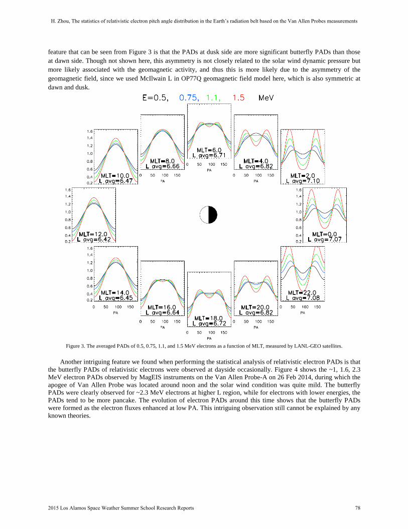
feature that can be seen from Figure 3 is that the PADs at dusk side are more significant butterfly PADs than those at dawn side. Though not shown here, this asymmetry is not closely related to the solar wind dynamic pressure but more likely associated with the geomagnetic activity, and thus this is more likely due to the asymmetry of the geomagnetic field, since we used McIlwain L in OP77Q geomagnetic field model here, which is also symmetric at dawn and dusk.

Figure 3. The averaged PADs of 0.5, 0.75, 1.1, and 1.5 MeV electrons as a function of MLT, measured by LANL-GEO satellites.

Another intriguing feature we found when performing the statistical analysis of relativistic electron PADs is that the butterfly PADs of relativistic electrons were observed at dayside occasionally. Figure 4 shows the ~1, 1.6, 2.3 MeV electron PADs observed by MagEIS instruments on the Van Allen Probe-A on 26 Feb 2014, during which the apogee of Van Allen Probe was located around noon and the solar wind condition was quite mild. The butterfly PADs were clearly observed for ~2.3 MeV electrons at higher L region, while for electrons with lower energies, the PADs tend to be more pancake. The evolution of electron PADs around this time shows that the butterfly PADs were formed as the electron fluxes enhanced at low PA. This intriguing observation still cannot be explained by any known theories.



Figure 4. The PADs of ~2.3, 1.6, and 1 MeV electrons on 26 Feb 2014 measured by MagEIS on the Van Allen Probe-A.

4.2. The empirical model of 10s to 100s of keV electron PADs in the inner radiation belt and slot region MagEIS instruments provide unprecedented clean measurements of 10s to 100s of keV electrons in the low L

region. Using data from MagEIS on the Van Allen Probes, an empirical model of 10s to 100s of keV electron PADs in the low L region is constructed. Figure 5 and Figure 6 show some examples of model results in the low L region with intriguing features. Figure 5 shows the averaged PADs of ~105, 235, and 460 keV electrons as a function of MLT in the inner radiation belt measured by MagEIS instruments during quiet geomagnetic activities (Dst > -20 nT). Note that in the inner belt, as expected, the averaged PADs have no dependence on MLT, indicating an azimuthally symmetric geomagnetic field in the low L region. The newly unveiled 90°-minimum PADs are clearly shown in the Figure 5 for different energy electrons. It is clear from Figure 5 that for electrons with higher energies the minimum at 90° PA tends to be more significant. At L=1.4 and 1.6, the minima at 90° PA are very clear; while as the L shell becomes higher, the minima at 90° gradually disappear. Though not shown here, during storm times with Dst < -20 nT, the averaged PADs in the inner belt have more significant minima at 90° PA. This is consistent with the observations from Zhao et al. [2014a, 2014b]. The wave-particle interaction of fast magnetosonic waves is suggested as a possible mechanism responsible for the formation of this PAD type, while the actual causes are still under debate. Though the formation of such 90°-minimum PADs is still not clear, the disappearance of this type of PADs at higher L shells is likely to be caused by the plasmaspheric hiss wave scattering [Zhao et al., 2014b]. Our model results also support this hypothesis, which shows as the cap PADs appear (indicating the presence of hiss wave scattering, as can be seen in the Figure 6) the minima at 90° disappear.

Figure 6 shows the averaged PADs of ~105, 235, and 460 keV electrons as a function of MLT in the slot region measured by MagEIS instruments during quiet geomagnetic activities (Dst > -20 nT). Similarly, no MLT dependence is observed in the slot region either. The cap PADs clearly show up in Figure 6. At L=2.2, the cap PADs are only present for ~460 keV electrons, while for ~105 and 235 keV electrons the PADs are more like pancake PADs. As L shell increases, the cap PADs can be observed for all energy electrons shown here, but the size of “cap” is smaller for higher energy electrons and larger for lower energy electrons. This is consistent with the theoretically



predicted PADs caused by plasmaspheric hiss wave scattering. It is also worth to mention that during geomagnetic active times (Dst < -20 nT) the averaged PADs in the slot region are mostly pancake PADs. This may indicate during active times, other physical processes, e.g., inward radial diffusion and wave heating, play more important roles on relativistic electron dynamics in the slot region than hiss wave scattering.

Figure 5. The averaged PADs of ~105, 235, and 460 keV electrons at different MLTs in the inner radiation belt, reconstructed from the statistical

relativistic electron PAD model during geomagnetic quiet times (Dst > -20 nT).



Figure 6. Similar format with Figure 5 but for results in the slot region.

5. Conclusions

A statistical study of relativistic electron pitch angle distribution using data from REPT, MagEIS instruments on the Van Allen Probes and LANL-GEO satellites is performed. An empirical model of radiation belt electron pitch angle distribution as a function of L, MLT, electron energy, and geomagnetic activity is developed and some interesting results are found. The conclusions of this study are as follows:

1) An unexpected dawn-dusk asymmetry of ultra-relativistic electron PADs is observed using data from REPT instruments on the Van Allen Probes, which is shown as more peaked pancake PADs at dusk than at dawn. This asymmetry is only observed for ultra-relativistic electrons and is more significant for electrons with higher energies. It is shown that this asymmetry is not just due to the asymmetry of geomagnetic field, and it is possibly related to the physical processes that can affect relativistic electron PADs on a timescale of drift period. Using data from LANL-GEO satellites which give simultaneous measurements at different MLTs at the geosynchronous orbit, this asymmetry cannot be clearly seen, which could be due to the limited energy range in LANL-GEO data.

2) Using LANL-GEO data, electron PADs at the geosynchronous orbit are investigated and a dawn-dusk asymmetry with more significant butterfly PADs at dusk than dawn is observed. This asymmetry, unlike the one observed by Van Allen Probes, is likely due to the asymmetry in the geomagnetic field.

3) Using data from MagEIS instruments, an empirical model of 10s to 100s of keV electron PADs in the inner radiation belt and slot region is constructed. It is shown that during geomagnetic quiet times, the 90°-minimum PADs in the inner belt are always observed, and the minima at 90° PA are more prominent for electrons with higher energies. In the slot region, the cap PADs are generally observed during quiet times and the dependence of the PAD shape on electrons’ energy and L shell is consistent with the theoretical prediction. However, during geomagnetic disturbed times, instead of cap PADs, the pancake PADs are commonly observed, which may indicate the more



important roles of other physical mechanisms, e.g., inward radial diffusion and wave heating, than the hiss wave scattering during geomagnetic storm times.

References

Baker, D. N., P. R. Higbie, E. W. Hones Jr., and R. D. Belian (1978), High-resolution energetic particle measurements at 6.6 Re 3. Low-energy electron anisotropies and short-term substorm predictions, J. Geophys. Res., 83 (A10), 4863-4868, doi:10.1029/JA083iA10p04863.

Baker, D. N., et al. (2013), The Relativistic Electron-Proton Telescope (REPT) Instrument on Board the Radiation Belt Storm Probes (RBSP) Spacecraft: Characterization of Earth’s Radiation Belt High-Energy Particle Populations, Space Science Reviews, doi:10.1007/s11214-012-9950-9.

Blake, J. B., et al. (2013), The magnetic electron ion spectrometer (MagEIS) instruments aboard the radiation belt storm probes (RBSP) spacecraft, Space Sci. Rev., doi:10.1007/s11214-013-9991-8.

Chen, Y., R. H. W. Friedel, M. G. Henderson, S. G. Claudepierre, S. K. Morley, and H. Spence (2014), REPAD: An empirical model of pitch angle distributions for energetic electrons in the Earth’s outer radiation belt, J. Geophys. Res. Space Physics, 119, 1693–1708, doi:10.1002/2013JA019431.

Gannon, J. L., X. Li, and D. Heynderickx (2007), Pitch angle distribution analysis of radiation belt electrons based on Combined Release and Radiation Effects Satellite Medium Electrons A data, J. Geophys. Res., 112, A05212, doi:10.1029/2005JA011565.

Horne, R. B., N. P. Meredith, R. M. Thorne, D. Heynderickx, R. H. A. Iles, and R. R. Anderson (2003), Evolution of energetic electron pitch angle distributions during storm time electron acceleration to megaelectronvolt energies, J. Geophys. Res., 108(A1), 1016, doi:10.1029/2001JA009165.

Horne, R. B., R. M. Thorne, S. A. Glauert, J. M. Albert, N. P. Meredith, and R. R. Anderson (2005), Timescale for radiation belt electron acceleration by whistler mode chorus waves, J. Geophys. Res., 110, A03225, doi:10.1029/2004JA010811.

Kessel, R. L., N. J. Fox, and M. Weiss (2013), The Radiation Belt Storm Probes (RBSP) and space weather, Space Sci. Rev., 179(1-4), 531–543, doi:10.1007/s11214-012-9953-6.

Li, W., Y. Y. Shprits, and R. M. Thorne (2007), Dynamic evolution of energetic outer zone electrons due to wave-particle interactions during storms, J. Geophys. Res., 112, A10220, doi:10.1029/2007JA012368.

Lyons, L. R., and D. J. Williams (1975a), The quiet time structure of energetic (35-560 keV) radiation belt electrons, J. Geophys. Res., 80 (7), 943-950.

Lyons, L. R., and D. J. Williams (1975b), The storm and poststorm evolution of energetic (35-560 keV) radiation belt electron distributions, J. Geophys. Res., 80 (28), 3985-3994.

Reeves, G., R. Belian, T. Cayton, M. Henderson, R. Christensen, P. McLachlan, and J. Ingraham (1997), Using los alamos geosynchronus energetic particle data in support of other missions, in Satellite-Ground Based Coordination Source Book, edited by M. Lockwood and H. Opgenoorth, pp. 263 – 272, Eur. Space Agency, Noordwijk, Netherlands.

Schulz, M., and L. Lanzerotti (1974), Particle Diffusion in the Radiation Belts, Springer, New York. Selesnick, R. S., and J. B. Blake (2002), Relativistic electron drift shell splitting, J. Geophys. Res., 107(A9), 1265, doi:10.1029/2001JA009179. Sibeck, D. G., R. W. McEntire, A. T. Y. Lui, R. E. Lopez, and S. M. Krimigis (1987), Magnetic field drift shell splitting: Cause of unusual

dayside particle pitch angle distributions during storms and substorms, J. Geophys. Res., 92, 13,485–13,497, doi:10.1029/JA092iA12p13485.

Tsyganenko, N. A. (1989), A magnetospheric magnetic field model with a warped tail current sheet, Planet. Space Sci, 37, 5. Tsyganenko, N. A., and M. I. Sitnov (2005), Modeling the dynamics of the inner magnetosphere during strong geomagnetic storms, J. Geophys.

Res., 110, A03208, doi:10.1029/2004JA010798. West, H. I., R. M. Buck, and J. R. Walton (1973), Electron pitch angle distributions through the magnetosphere as observed on Ogo5, J. Geophys.

Res., 78, 1064–1081. Zhao, H., X. Li, J. B. Blake, J. F. Fennell, S. G. Claudepierre, D. N. Baker, A. N. Jaynes, D. M. Malaspina, and S. G. Kanekal (2014a), Peculiar

pitch angle distribution of relativistic electrons in the inner radiation belt and slot region, Geophys. Res. Lett., 41, doi:10.1002/2014GL059725.

Zhao, H., X. Li, J. B. Blake, J. F. Fennell, S. G. Claudepierre, D. N. Baker, A. N. Jaynes, and D. M. Malaspina (2014b), Characteristics of pitch angle distributions of hundreds of keV electrons in the slot region and inner radiation belt, J. Geophys. Res. Space Physics, 119, 9543–9557, doi:10.1002/2014JA020386.



Los Alamos Space Weather Summer School 30 Bikini Atoll Rd, ISR-1, MS D466 Los Alamos, NM 87545 http://swx-school.lanl.gov

los alamos space weather summer school research reports€¦ · 2015 los alamos space weather...

Documents