NASA Technical Memorandum 107006

E,--C)j89 1/ /1;-

Low-Order Nonlinear Dynamic Model of Ie Engine-Variable Pitch Propeller System for General Aviation Aircraft

Jacques C. Richard Lewis Research Center Cleveland, Ohio

July 1995

National Aeronautics and Space Administration

https://ntrs.nasa.gov/search.jsp?R=19950026495 2018-07-23T12:58:14+00:00Z

..

LOW-ORDER NONLINEAR DYNAMIC MODEL OF IC ENGINE-VARIABLE PITCH PROPELLER SYSTEM FOR GENERAL A VIATION AIRCRAFT

by

Jacques C. Richard* NASA Lewis Research Center, Cleveland, Ohio 44135

This paper presents a dynamic model of an internal

combustion engine coupled to a variable pitch propeller. The

low-order, nonlinear time-dependent model is useful for

simulating the propulsion system of general aviation

single-engine light aircraft. This model is suitable for

investigating engine diagnostics and monitoring and for

control design and development. Furthermore, the model may

be extended to provide a tool for the study of engine

emissions, fuel economy, component effects, alternative fuels,

alternative engine cycles, flight simulators, sensors and

actuators. Results presented in this paper show that the model

provides a reasonable representation of the propulsion system

dynamics from zero to 10 Hertz.

Introduction

This paper presents a General Aviation (GA) propulsion system model that is suitable for diagnostics

and engine monitoring, for control and design studies, and for flight simulators. The model is developed

1 Aerospace Engineer

1

by adapting a low-order, nonlinear, dynamic model of an internal combustion (IC) engine produced for the

automotive industryl, 2 to GA use. The GA engine system model is then coupled to a variable-pitch

propeller model to obtain the full GA propulsion system model.

The model presented in this paper is a first step toward advancing the state-of-the-art in GA engine

systems. The GA industry has been producing light aircraft for many years. However, dynamic models of

the relatively simple single-engine propulsion systems are still widely nonexistent. Aerospace research has

tended to focus on the turbojet and turbofan engines used by the larger commercial airlines. This has

allowed many improvements to be made in the engine systems of larger aircraft while almost totally

ignoring the GA industry.

The lighter GA planes typically have internal combustion engines similar to those used in automobiles.

The automobile industry has made many advances in dynamic modeling of these engines, especially in the

study of emissions, efficiency, advanced sensors and controls. However, none of these advances have

made their way into the GA industry. The model presented in this paper is a first attempt to use the

advances in automotive engine modeling to improve GA engine systems.

This paper presents a low-order, nonlinear, dynamic model of an internal combustion engine coupled

to a variable pitch propeller propulsion system for GA aircraft in the following manner. First, a model of

the variable pitch propeller is obtained3. Next, an engine model is developed that is based on low order

engine torque and speed models as applied to automobiles 1, 2. This model of the engine uses a steady-state

engine performance map that contains the end result of the combustion, piston motion, engine cranking

and exhaust rather than model these processes in detail for the simplicity of a preliminary model. Third, a

model of the intake process is developed using low order models of the manifold, throttle and fuel flow

rates1, 2, 4, 5. The intake process is also modeled with an intake map rather than in detail. Conservation of

2

..

mass equations are used to ensure that the simple model obeys conservation principles. One of the inputs

for this propulsion system model is altitude. Therefore, a model of atmospheric variation with altitude is

also presented 6, 7. These models are integrated into the overall GA propulsion system model that is then

placed in state-variable form for implementation.

The mathematical description of the model is followed by the results of simulations with varying model

inputs (blade pitch, throttle angle and fuel to air mixture ratio -- separately and in different combinations).

The first three cases show the result of varying each of the inputs individually. The fourth case presents

results for simultaneous throttle and blade pitch commands to the engine. A final case investigates the

result of combining all three inputs. These last two cases are examples of how a single lever power control

(SPLC) system might be implemented.

Variable Pitch Propeller Model

The model begins with the GA aircraft's variable pitch propeller that moves air backwards to get the

reaction force, the thrust, to move the plane forward. The propeller model assumes3 that the whole

propeller acts as an airfoil, the total area of which is assumed concentrated at a certain distance, r gy' from

the flight or propeller axis. The blade element is at an angle, /3, from the plane of rotation. The net motion

is a combination of an axial translation with velocity, V, and a rotation with angular speed, (i) = 2 1r N /

60. All the blades are thus replaced by one blade element at a distance, rgy from the shaft, (note that this

representation made rgy the radius of gyration, rgy = rprop /"';2 and rprop = 3.5 ft), on which is based a

propeller disk area, Aprop = 1r rgy2. This approach has been called the method of representative blade

element3. This strictly theoretical method yields general information about propeller characteristics. It is

chosen because of the lack of available data for particular propeller behavior -- besides, this propeller

3

model may be said to be more broad and generic this way. The chord line is used to represent the propeller

section. The chord line forms an angle, /3, with the direction of rotational velocity, r x co. The resultant

velocity, which tends an angle, 13 - a, with the chord line, making this angle the blade pitch, has the

magnitude V I sin (13 - a) = rgy rol cos (13 - a). The propeller is then found to provide a thrust3

1 [rOJ)2 r prop ( 13 - a, ro, P a' r) = [ C L COS ( 13 - a) - CD sin ( 13 - a) ] 2: P a A prop CoS( 13 _ a)

(1)

that is also dependent on altitude, H, through the ambient air density, Pa. The propeller torque is similarly

found to be3

1 [rOJ)2 Q proi 13 - a, OJ, P a' r) = [C L sine 13 - a) + CD cos ( 13 - a) ] 2: P a A prop cos ( 13 _ a) r

(2)

where

CL ( 13 - a) = 0.1 (13 - a) (3)

and

CD ( 13 - a) = 0.02 ( 13 - a) + 0.002 ( 13 - a)2 (4)

are empirical lift and drag coefficients, respectively3. When the propeller torque is multiplied by the

angular velocity, OJ, the propeller power, P prop' is obtained.

P prop( 13 - a, co, Pa,r)= Q prop( 13 - a, ro, Pa' r) ro (5)

4

The propeller torque represents the propeller loading on the engine. The propeller power is the amount of

power that the engine needs to be able to supply. Notice that the propeller torque and power both depend

on propeller-engine shaft speed, pitch, and altitude through the air density. The engine torque and power

needed to handle the propeller load will be discussed in the following section on the engine model. The

model of the process by which air and fuel get delivered to the engine to generate the needed torque and

power is also discussed.

Engine Model

In General Aviation, air-cooled, internal combustion, reciprocating piston engines are typically used to

drive the propeller. The model of the engine presented in this paper is kept simple by looking at the engine

as a whole and not looking in detail into the combustion process nor the link between the pistons and the

crankshaft. What helps to keep the model simple and focused on the global behavior of the engine­

propeller system is that engine manufacturers have maps of engine performance characteristics8. This

allows for a macroscopic level of engine modeling. Thus, in this model, the reciprocating engine's internal

combustion cycle is assumed inherent in the engine maps allowing for a simple assumption of engine

dynamic response.

The map used in this work represents the model 10-470 engine made by Teledyne Continental

Motors8. The map is the only engine-specific part of the model, all other terms in the equations that do not

contain the map subscript are generic. The 10-470 engine has six horizontally opposed cylinders (Le., flat

six arrangement) and can go up to 220 BHP at 2550 RPM.

5

Engine Torque and Power

Engine characteristics for piston-engined aircraft are typically arranged in performance maps that relate

important engine variables to parameters representing the environment within which the engine operates 8 ,

9. Therefore, many details of the torque and power process are not modeled. The maps provide a way of

obtaining the torque and power produced by the engines for various air conditions, engine speeds, and

injection system settings. The torque that the engine produces should then balance that which the propeller

requires to move the plane. Thus, the engine can simply be modeled macroscopically as a supplier of a

torque according to a given engine map. The particular engine map used here relates engine brake specific

fuel consumption, engine power, and speed. Using the definition of the brake specific fuel consumption,

torque, engine speed, fuel flow, and engine torque, the torque that the engine can produce according to the

map is

550 WI Qe. map ( wI' N, Qe ) = --:-\---------=Q---:-\--tc-..:..-

BSFC (N ,N 3~ 55~) map 30 N (6)

The engine cannot instantaneously produce Qe. map' as given above. A finite response time is

assumedl,2 for the engine to produce a torque, Qe, to satisfy the propeller needs via Qprop. This response

time may be assumed l , 2 to be related to the cycle as 'Ie = 60/ N. That is to say that the engine cycle, with

its intake, combustion and exhaust processes inherent in the map, may then have a simple first order

response

Qe = + [ Qe. map ( wI' N, Qe) - Qe ]. e

(7)

6

Engine Speed

A torque balance on the short crankshaft, on which the propeller is assumed to be mounted, can supply

the engine speed equation. The dynamics of the crankshaft itself are not significant compared to larger

components like the propeller (lprop = 1C rprop4 12 ). The equation for this balance is

(8)

Fuel Flow

Because controlling fuel flow is important in controlling the engine, the induction process is modeled.

The modeling of this process begins with the fuel injection system. The fuel injection system may be

designed to have the flow rate proportional to an injection pulse width commandl, 2. To maintain the

simplicity of the system, the actual flow rate is assumed to have a first order relation to the commanded

fuel flow rate1, 2.

(9)

The fuel flow time constant is arbitrarily taken to be 'rj = 0.5 sec, a typical value 1,2. The commanded fuel

flow rate on the right hand side of (9) is taken to be the weight flow past the throttle plate multiplied by the

fuel-air mixture ratio commanded by the pilot, (FIA)c, as in

where

(10)

This equation contains the conversion factor, g, to convert mass units from slugs to Ibm. This term also

contains the discharge coefficient, Cdchrg, estimated conservatively to be a low 0.6 although it could be

dependent on other flow parameters (complications not yet of interest). The throttle area through which the

7

flow passes the throttle plate depends on the throttle plate angle commanded by the pilot, 9c and is given

by 6,7

(11)

D2 cos ( 9c + 9s ) • -1 ~ (d ___ C....,....O_S _9s--,-_]2 -- sm 1--2 cos 9 s D cos ( 9 c + 9 s )

This equation shows how throttle flow cross-section varies with throttle angle (and so, shows how the

flow past the throttle plate varies with throttle plate angle). The commanded throttle angle, 90 can range

from a set reference angle taken here as, 9s = 0, up to 70° for the model 10-470 series engine. The

dynamics of the throttle plate are ignored as they are assumed of a higher frequency than the more massive

components whose dynamics are of greater interest. The mass flux through the throttle area is given by 6,7

Pa ( :. r ~ 2r [ 1 _ --L ]-7 , --L > ( 2

) T~I ,J RTa r- 1 Pa Pa r+1

c:p ( P man' P a' T a ) =

~r( )~ ~ ( 2 ) Y~I Pa 2 y-I --L

~ RTa r+1 Pa r+1 (12)

This term shows the dependency on altitude given that Pa and Ta both depend on altitude. If P > P (b then

the flow past the throttle plate is subsonic otherwise that flow is choked. Given (10), (9) may be written as

(13)

8

Intake Manifold Pressure

The manifold pressure is assumed to respond in a first order fashion when changes in torque and

power get requested from the engine, as with other subsystems modeled here. The pressure that the intake

manifold would respond to in this manner is a characteristic of the engine specified by the intake manifold

pressure map for the engine,

Pman. map( Qe , N ) = Pman. map ( Qe * N * 7r / ( 30 * 550 ) , N ) (14)

giving

. 1 P man ( Qe ' N ) = -'t'- [ P man, map ( Qe , N ) - P man ].

man (15)

Intake Manifold Flow

Conservation of the mass within the intake manifold is insured with an equation obtained for a balance

of the mass flowing across a control volume around the manifold. Accumulation of mass in the manifold

is assumed of first order, therefore

1 W man = -- {w f - W man + W th ( e c' P man' P a' Ta) }.

't'man (16)

This equation balances any accumulation of air and fuel in the manifold with the net weight flow rates of

fuel, of the intake manifold and of air past the throttle plate, respectively. In this equation, the time

constant for the intake process is taken to be half the engine time constant, 't'man = 't'e /2 = 60/2 N. This is

because for this macroscopic level of modeling, the complete intake and exhaust are assumed to occur

sequentially, with similar amounts of mass, within the cycle and so share the cycle time. The exhaust

manifold flow is not modeled here because it is assumed to have negligible effects in the simple model.

9

Altitude Effects

The engine model naturally depends on the atmospheric conditions (Pa> Ta and Pa ). Standard air

conditions are assumed for this analysis. Parkinson6, 7 lists the equations that approximate the

characteristics of the U. S. Standard Atmosphere (1962) model in the troposphere.

; = 1 - 6.8729(10-6) H (17)

~ = ;5.25581 (18)

(J'= Pa I Pa, SeaLevel = ~/; (19)

Ta = 530; (R) (20)

Pa = 29.92 ~ (in Hg) (21)

Next, the altitude model is incorporated into the whole GA propulsion system model in state variable

form. This form is one that is merely convenient for this effort.

State Variable Form

The propulsion system model is made easier to implement by putting it in state variable form, a form

useful for control design. The coupling of the various engine and propeller components also becomes

more obvious in this form. By defining

Xl =N

X2= Qe

X3 = Pman

X4 = Wman

X5 = WI

10

equations (7), (8), (14) and (16) can be rewritten as

30 X j = 7r I [ X 2 - Qprop ( X j , f3 - a, P a ) ]

prop

1

[Pman,map(X j , X 2 ) -X 3 ]

(22)

(23)

(24)

(25)

(26)

Figures 1 and 2 show the model in block diagram form. Here, the inputs are blade pitch, in f3 - a,

throttle angle command, Be, fuel to air mixture ratio, (F / A)e, and altitude. The outputs are propeller and

engine power; speed; manifold pressure; mixture ratio; and fuel flow. Using these forms, several cases

are simulated and the results are discussed next.

Simulation Results

The simulation results that follow are from a set of inputs and initial conditions typical of a cruising

GA plane like the T34B equipped with the IO 470 engine modeled here. These simulations follow a

transient to settle to a steady state cruise condition. After reaching a the steady-state condition, some

variations are imposed -- variations in blade pitch, mixture ratio, throttle opening, each separately; then

11

blade pitch and throttle opening together; and finally, all three simultaneously. This is to investigate the

system response to each input and combinations of inputs. Linear analyses of the simulations show a

bandwidth of 0 to 10 Hertz.

A low altitude cruise condition is first simulated. The initial conditions are: X](O) = N(O) = 2000

RPM, X2(0) = QlO) = 304.6 lb-ft, X3(0) = Pman(O) = 24 in Hg, X4(0) = w'man(O) = 913.5 lbmlhr and

Xs(O) = wiO) = 60.9 lbmlhr. The inputs are: f3 - a = 00, Be = 33°, F / A = 1/15 = 0.0667, andH =

6000 ft. The outputs are propeller horsepower, engine horsepower, engine speed, manifold pressure,

mixture ratio, and fuel weight flow rate. The output mixture ratio is calculated as

or

F A

F A

Varying Cruise Inputs

(27)

(28)

Once reaching a steady state cruise condition with the cruise inputs and initial conditions, a step change

in one of the inputs is imposed. A blade pitch step change is the first case simulated.

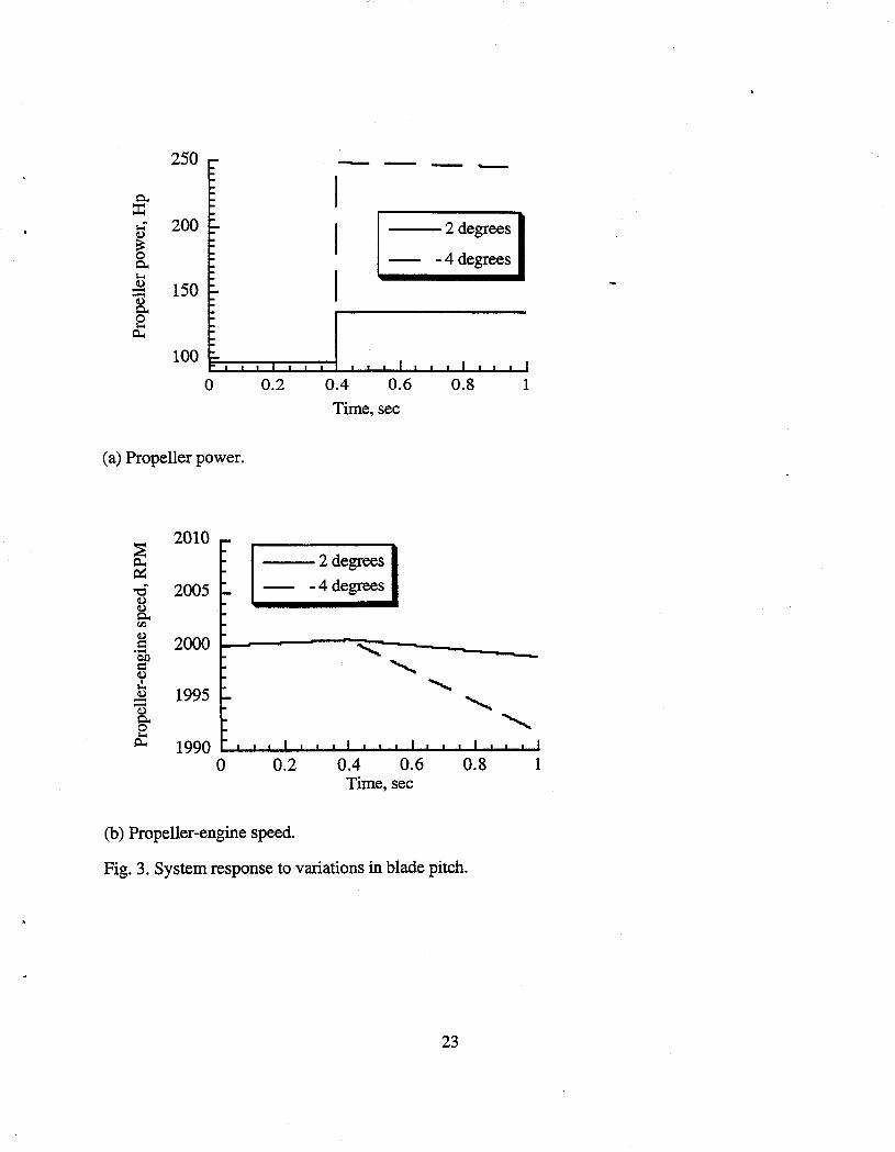
Blade Pitch

The blade pitch is given a step increase from O· to 2° and a step increase from O· to 4· each starting

from steady cruise. The results of each blade pitch step increase are plotted together in Fig. 3. The dashed

curve shows the 4· case. In this case, the propeller horsepower goes quickly to a steady-state after the step

change (Fig. 3(a». Since the engine is not being supplied any fuel to provide the power required, the

propeller-engine speed decreases (Fig. 3(b)). The manifold pressure decreases slightly until it reaches

12

steady state but it is not influenced by the blade pitch (Fig. 3(c)). Meanwhile, the resultant mixture ratio

hardly changes from the steady-state cruise condition (Fig. 3(d», since the other flow rates show little

change. Fuel flow decreases because, as the engine speed decreases, so do the flow requirements (as the

manifold pressure show, Fig. 3(c», it takes longer to change from steady-state cruise and reach a new

steady state (Fig. 3(e».

In the 4° blade pitch case, the same behavior happens but more pronounced since this is a higher blade

pitch. However, since the step is larger, the engine speed takes longer to reach steady state due to the

inertia of the propeller. Again, the other engine parameters simply go to steady state without any influence

of blade pitch. The propeller relationships are mostly quadratic in blade pitch but this case shows the

greater influence of the linear part of these relationships (the coefficient of the quadratic part being very

small).

Fuel to Air Mixture Ratio

The fuel to air mixture ratio is given a step increase from stoichiometric to 0.07667 in this case and a

step increase from stoichiometric to 0.8667, again each starting from steady cruise. Everything increases

in this case except the air flow (Fig. 4). The fuel flow increases before the other flow rates (Fig. 4(e»

since fuel flow has a shorter response time. This causes the resulting mixture ratio to increase (Fig. 4(d».

Increases in fuel cause increases in engine power (Fig. 4(a», consequently, engine speed increases (Fig.

4(b». As a further consequence, manifold pressure increases with engine power and speed (Fig. 4(c».

Throttle Angle

The throttle is opened by stepping the throttle plate angle from 33° to 43° in one subset of this case and

33° to 53° in another subset of this case. The response to the throttle being opened is a higher fuel and air

flow rate into the engine (pressure inside the manifold being lower than outside). As a result, the engine

generates more power (Fig. 5(a». The fact that the 53° case power curve shows a slope different from the

13

43° case implies a nonlinearity in response time. Engine power increases faster than the previous cases.

Engine speed increases (Fig. 5(b)). Manifold pressure increases faster than other cases because it depends

on engine power and speed (Fig. 5(c)). Opening the throttle allows more air and fuel into the engine and

so engine power increases faster with increased fuel flow. However, propeller-engine speed does not

increase that fast because of the propeller inertia. Unlike the others, fuel to air mixture ratio shows a step

(Fig. 5(d)) due to the difference in the response time of the fuel and the manifold flow rates. But the

mixture ratio does eventually return to its initial value, apparently at the slower rate of manifold flow than

that of the fuel flow (Fig. 5(e)). This occurs with the fuel and air flow rates seeming to eventually negate

each other's effects on mixture ratio as mixture ratio reaches the same steady state for both cases. This

implies a nonlinear response in flow rates to throttle changes.

Blade Pitch and Throttle Angle

The previous variations in each of the blade pitch and throttle opening cases are coupled in this case.

The shape of the curves in Fig. 6 shows shapes from the increasing blade pitch curves (Fig. 3) and the

increasing throttle angle curves (Fig. 5). Elements of the individual cases show up in this combined input

case. Propeller and engine power increase due to the increase in blade pitch and throttle angle, respectively

(Fig. 6(a)). Engine speed increases with 43° throttle opening since the increased fuel into the engine is

enough to allow the engine to handle the increased loading of the 2° blade pitch case (Fig. 6(b)). But the

increased fuel that comes with the 53° throttle opening is not enough for the 4° blade pitch case. Manifold

pressure increases as in the previous throttle angle case (Fig. 6( c)) -- not effected by the other input

changes. Fuel to air mixture ratio does not change with blade pitch before but shows some of the dynamic

behavior of the increased throttle angle case in this case with the coupled inputs (Fig. 6(d)). Fuel flow

increases quickly due to the throttle angle increase (Fig. 6(e)).

14

Blade Pitch, Throttle Angle and Fuel to Air Mixture Ratio

A similar type of coupled output from coupled input results here (Fig. 7) as in the previous case but

more pronounced when the effects of mixture ratio are included. This is good since a lot of engine power

is needed to handle the propeller loads via the blade pitch changes -- but even that is not enough for the 4 0

blade pitch load. In the results of the coupled inputs, propeller and engine power increase (Fig. 7(a».

However, engine. speed decreases with the higher throttle opening and mixture ratio because the increased

loading of the higher blade pitch was still too great (Fig. 7(b». Similarly, manifold pressure increases with

the coupled blade pitch, throttle angle and mixture ratio increases (Fig. 7(c». The resulting mixture ratio

increases since it is set to increase and because of opening the throttle (Fig. 7(d». Fuel flow increases with

mostly the rates associated with opening the throttle dominant (Fig. 7(e».

The coupled blade pitch, throttle angle and mixture ratio case shows how engine and propeller power

can increase with simultaneous increases of all three inputs. These last two cases demonstrate that the

model could be used to develop a single lever power control system for GA airplanes. The way they

would be varied depends on the particular aircraft, propulsion system and control design.

Concluding Remarks

A low-order, nonlinear, dynamic model of an internal combustion engine coupled to a variable pitch

propeller is constructed for general aviation (GA) single-engined light aircrafts. The results show that the

model captures internal combustion engine and variable-pitch propeller dynamic behavior as in other

research on automotive reciprocating engines. Linear analyses of the simulations show a bandwidth of 0 to

10 Hertz. The model is suitable for control and design studies. Furthermore, the results show how the

GA airplane propulsion system may respond with a single lever power control system.

The model however is limited to global, low-order dynamic Ie engine-variable pitch propeller system

behavior since that is a major assumption. General Aviation aircraft propulsion system data is limited and

15

therefore a flight-test is needed to validate the model. Aspects of the model requiring validation include the

maps, the propeller relationship, and the response times. More detailed modeling of individual components

and processes should also provide refinements of the maps, propeller relationship, and assumed response

times . Details of the combustion process, intake and exhaust throughout the cycle could provide more

elaborate data on the timing effects as well as on emissions and fuel economy, the effects of various

alternative fuels and even other engine cycles. Such details could also provide a better understanding of the

coupling of power, speed, manifold pressure and flow rates. Details of actuator dynamics, additional

sensor and control mechanisms could also be included in the model.

16

Nomenclature

A Area (sq. ft. or sq. in., specified for appropriate equation).

BHP Brake horsepower from engine maps (hp).

BSFC Brake specific fuel consumption (BSFC = Fuel Flow / BHP , IblBHP hr). Also SFC.

C Coefficient.

D Throttle bore diameter of3.25 in.

d Throttle rod diameter 0.38 in.

F / A Fuel to air mixture ratio.

g Conversion factor for converting slugs to Ibm.

H Altitude (ft).

I Moment of inertia (in4).

N Engine speed (RPM for revolutions per minute).

P Power (lb-ftls).

p Pressure (in Hg).

Q Torque (lb-ft), e.g., Qe, map = BHP * 550/( RPM * 1! /30) = P e, map * 550/( Ne, map * 1C /30 ) .

R Gas constant (ft2 / s2).

RPM Engine speed from engine maps (Revolutions Per Minute).

r Radius (ft).

SFC Specific fuel consumption from engine maps (lbIBHP hr). Also BSFC

T Thrust (lbs).

Ta Ambient air temperature (R).

V Propeller resultant velocity (ftls).

w Weight (lb).

X State variable for a which a subscript specifies a state.

17

Greek characters

a Propeller angle of attack (degrees).

f3 Propeller angle with plane of rotation (degrees).

r Ratio of specific heats of air.

¢> Mass flux (lb/hr/in2).

f) Throttle angle (degrees).

p Density (slugs/ft3).

(J Term used in showing atmospheric variation with altitude.

Time constant (sec).

Angular velocity (rad/s).

~ Term used in showing atmospheric variation with altitude.

, Term used in showing atmospheric variation with altitude.

18

Subscripts

a Ambient air conditions.

c Command as in commanded value.

D Drag.

dchrg Discharge as in discharge coefficient.

e Pertaining to the engine.

f Pertaining to the fuel.

gy Gyration as in radius of gyration.

L Lift.

man Pertaining to the intake manifold.

map Pertaining to the engine maps.

prop Pertaining to the propeller.

th Pertaining to the throttle.

s Set as in set throttle angle.

19

References

lPowell, B. K., "A Simulation Model of an Internal Combustion Engine-Dynamometer System", Ford

Motor Co., Dearborn, MI

zPowell, B. K., "A Dynamic Model for Automotive Engine Control Analysis", IEEE, pp. 120-126, 1979.

-3von Mises, Richard, Theory of Flight, Dover, New York, 1959.

4Moskwa, J. J. and Hedrick, J. K., "Modeling and Validation of Automotive Engines for Control

Algorithm Development", Transactions of the ASME, Vol. 114, pp. 278-285, June 1992.

5Moskwa, John J., "Automotive Engine Modeling for Real Time Control", Ph. D., Thesis, MIT, 1988.

6Parkinson, R. C. H., "An operational Model of Specific Range for Microprocessor Applications in

Piston-Prop General Aviation Airplanes", AIAA 81-2330, 1981.

7Parkinson, Richard C. H., "A Fuel-Efficient Cruise Performance Model for General Aviation Piston

Engine Airplanes", NASA-CR-172188, N83-33891, Ph. D. Thesis, Final Report, Princeton University,

August 1983.

8Teledyne Continental Motors, Corp., "Detail Specification for Continental Aircraft Engines Model 0-470-

4", Teledyne Continental Motors, Corp., Aircraft Engine Division, Muskegon, MI.

9Bent, Ralph D. and McKinley, James L., Aircraft Power plants, 4th ed., McGraw-Hill, NY 1978.

20

r Pilot­Inputs

..." --II Engine

II

" Fuel System uell ~ir II RatIo

F

II

II Air

II Throttle

Throttle 'I" Body c ommandll

Figures

Fuel I Flow Engine Power - & Torque

Torque I Power , Manifold Pressure

~

Inertia IL- - - ~- -- - -Propeller I Toraue I I Propeller ..

Blade I Torque PItch L __ _

Fig. 1. Summary diagram of modeL

21

-r;--I System

I I Outputs

1 II -.....

Fue

.-11 Flo w

- II

,I

+- ITMani fold sure

-

I' Pres

d II Engi I Spe

ne ed

I , Pil ot ges - -I

Ga -

Blade Pitrh ..

Alti tude Propeller - + .. Torque or .. 'l'e, Engine

En gine ~/I p S Time Constant

Speed 60/N .. - Engin e

ue Torg , Fuel FJow ... 1/('l'e s + 1) -

Engine Map ..

r-+- ... BSFC(BHP ,RPM) BSF ~

... Engine Engine

Engine Speed

Speed ,r Speed" ,r 'l'man, Manifold 160/2N I Manifold

Engine Manifold Pressure Time Constant Pressure Map --e. 1 / ('l'man s+l)

Pman(BHP,RPM) 4

Manifold Pressure

L. , Ath(8c )

1 /('l'man s+l) .. Altitude- Throttle + -.. *(/J(Pman,alt)

AirFlow + Manifold Throttle Mass Flo w

Command r Fuel Flow Fuel! Air Ratio 0-+ l/('l'fs+l)

Fig. 2. Detailed diagram of the GA IC engine-variable pitch propulsion system dynamic model.

22

250 - - -0.-:I: ..: 200 2 degrees 11)

~ 0 -4 degrees 0.-I-< 0 150 --11)

0.-0 I-< ~

100

0 0.2 0.4 0.6 0.8 1 Time, sec

(a) Propeller power.

~ 2010

~ --- 2 degrees

-d' 2005 11)

-4 degrees 11)

0.-(I)

11)

2000 c .-bO C 0 I

I-< 1995 11) --11)

0.-

J: 1990 0 0.2 0.4 0.6 0.8 1

Time, sec

(b) Propeller-engine speed.

Fig. 3. System response to variations in blade pitch.

23

30

b1) 2 degrees r= 28 -4 degrees

e ~ 26 CIJ CIJ (!) I-! Q..

24 "0 -t8 '-0

C 22 ~

:E 20

0 0.2 0.4 0.6 0.8 1 Time, sec

(c) Intake manifold pressure.

0.1 2 degrees

0 .~ 0.08 -4 degrees I-!

e .a 0.06 x '8 I-! 0.04 '-0 ~

S - 0.02 (!) ~ ~

0 0 0.2 0.4 0.6 0.8 1

Time, sec

(d) Fuel to air mixture ratio.

Fig. 3. Continued.

24

120

110

'"' ~ 100 .0

90 -'i --2 degrees

-4 degrees

0 SO t;:::: -0 70 ::s ~

60

50 0 0.2 0.4 0.6

Time, sec

(e) Fuel weight flow rate.

Fig. 3. Continued.

240

0- 220 ::t:: 200 .: 0

ISO ::=

--F/A=.07667 - FI A=.OS667

0 0- 160 0 c

140 .-OJ) c ~ 120 --100

0 0.2 0.4 0.6 Time, sec

(a) Engine power.

O.S 1

-- - -

0.8 1

Fig.4. System response to variations in fuel to air mixture ratio.

25

:E 2010 -

~

" '" -d' 2005 -(I.)

--F/A=.07667 - FI A=.08667

(I.) 0.. <Il Q,)

2000 -Q .-b.() Q '" Q,) ;!..

1995 i-Q,) - i--Q,) 0..

£ 1990 I I I I

0 0.2 0.4 0.6 0.8 1 Time, sec

(b ) Propeller-engine speed.

30 b.() F/A=.07667

Et: 28 - FI A=.08667 2i ::s 26 <Il <Il

~ 0..

"0 24 -.E .-Q 22 ~

:E 20

0 0.2 0.4 0.6 0.8 1 Time, sec

(c) Manifold pressure.

Fig.4. Continued.

26

0.1

0 .- O.OS ~ 1-0

----e ::s 0.06 .... >< ·s 1-0 0.04 .-~ .8

--F/A=.07667 - FI A=.OS667

- 0.02 Q) ::s

Il...

0 0 0.2 0.4 0.6

Time, sec

(d) Fuel to air mixture ratio.

120

110 1-0

100 --F/A=.07667 .:e

ell ..0 - 90 ~ 0 SO c -Q)

70 ::s Il...

60

50 0 0.2

(e) Fuel weight flow rate.

FigA. Continued.

- FI A=.OS667

--f A 0.6

Ime, sec

o.S 1

---o.S 1

27

240 43 degrees

0.. 220 - 53 degrees

::I: 200 I-.:' 0

180 ---~ .,.",. 0 0.. 160 0 c:

140 .-b.O c: Q;l 120

100

0 0.2 0.4 0.6 0.8 1 Time, sec

(a) Engine power.

~ 2010

c:.:: -d' 2005 0

--- 43 degrees - 53 degrees

0 Q.. til

0 2000 c: .-b.O

c: 0

I I-<

1995 0 --0 Q..

8 c.. 1990

0 0.2 0.4 0.6 0.8 1 Time, sec

(b) Propeller-engine speed.

Fig. 5. System response to variations in throttle angle.

28

30 43 degrees OJ)

r= 28 - 53 degrees

~ ::l 26 en en e ---0.. ,-'0 24 -~ .-s::: 22 ~

::E 20

0 0.2 0.4 0.6 0.8 1 Time, sec

(c) Manifold pressure.

0.1

0 .- 0.08 ~ I-<

---43 degrees -53 degrees

e ::l 0.06 ..... :< ·8

I-< 0.04 ·ca 0 ..... - 0.02 (1)

~

0 0 0.2 0.4 0.6 0.8 1

Time, sec

(d) Fuel to air mixture ratio.

Fig. 5. Continued.

29

120

110 ~ 43 degrees

-E 100 -- 53 degrees ",-en ....... ,D - 90 ~ 0 80 t;:: -<I) 70 ~

60

50 0 0.2 0.4 0.6 0.8 1

Time, sec

(e) Fuel weight flow rate.

Fig. 5. Continued.

0-::r: ~ <I)

~ 0 ~

-- Propeller, 2 degrees pitch & 43 degrees throttle - Propeller, 4 degrees pitch & 53 degrees throttle

- - - Engine, 2 degrees pitch & 43 degrees throttle - - - - - Engine, 4 degrees pitch & 53 degrees throttle

240

220

200

180

160

140

120

100

0

, I

,-­"I ... ____ fI"

0.2 0.4 0.6 Time, sec

-,.-­~ ,."

0.8 1

(a) Propeller and engine power.

Fig. 6. System response to variations in blade pitch and throttle angle.

30

:E 2010 r-

~ ~ 2 degrees pitch & 43 degrees throttle

'ti 2005 I-- 4 degrees pitch & 53 degrees throttle

Q) Q)

~ 0.. en Q)

2000 s:: ........ .... 0.0 s:: '-Q)

~ """'-. I ~

1995 --Q) I- ---- ~ Q)

e ~ ~

p., 1990 .. i I I I • I I I I

0 0.2 0.4 0.6 0.8 1 Time, sec

(b) Propeller-engine speed.

30

0.0 --- 2 degrees pitch & 43 degrees throttle - 4 degrees pitch & 53 degrees throttle r= 28

e-o 26 en en 2 0..

"t:l 24 -..8 .... s:: 22 ~

:E 20

0

(c) Manifold pressure.

Fig. 6. Continued.

--0.2 0.4 0.6 0.8 1

Time, sec

31

0.1

0 .- 0.08 ..... ~

--2 degrees pitch & 43 degrees throttle - 4 degrees pitch & 53 degrees throttle ..

e :s 0.06 ..... x ·S .. 0.04 .-~ .9 - 0.02 ~

&! 0

0 0.2 0.4 0.6 0.8 1 Time, sec

(d) Fuel to air ratio.

120

110 --2 degrees pitch & 43 degrees throttle

- 4 degrees pitch & 53 degrees throttle .. 100 c:e -Vl ..c 90 -"i

0 80 t+=: -~ 70 tf 60

50 0 0.2 0.4 0.6 0.8 1

Time, sec

(e) Fuel weight flow rate.

Fig. 6. Continued.

32

-- Propeller, 2 degrees pitch, 43 degrees throttle & F/A=.07667 - - Propeller, 4 degrees pitch, 53 degrees throttle & FI A=.08667 - - - Engine, 2 degrees pitch, 43 degrees throttle & F/A=.07667 - - - - - Engine, 4 degrees pitch, 53 degrees throttle & FI A=.08667

;- - - -- --240 :-

I -220 -- .. ---" 200 :- .. -

0.. I .. . :I: - ,.

180 - f'

" .... - , 11,) 160 - I

, ~ - -, -0 I --~ 140 ;;.. • oi-

I ,

120 .... ./ ~----- ".

100 i-• I • I I

0 0.2 0.4 0.6 0.8 1

Time, sec

(a) Propeller and engine power.

2 degrees pitch, 43 degrees throttle & F/A=.07667 - 4 degrees pitch, 53 degrees throttle & F/A=.08667

~ 2010

~ -d' 2005

11,) 11,) 0.. Vl

11,)

2000 s= ""-.-co --s= 11,) -I -- -1-0 11,) 1995 --11,) 0.. 8 ~ 1990

0 . 0.2 0.4 0.6 0.8 1 Time, sec

(b) Propeller-engine speed.

• Fig. 7. System response to variations in blade pitch, throttle angle and fuel to air mixture ratio.

33

-- 2 degrees pitch, 43 degrees throttle & F/A=.07667 - 4 degrees pitch, 53 degrees throttle & FI A=.08667

30

OJ)

~ 28

e ~ 26 ell ell e 0..

"tj 24 -~ .-s:: 22 c<:S

~

20 0

(c) Manifold pressure.

0.2

I

..,.... /

-- -

0.4 0.6 0.8 1 Time, sec

--2 degrees pitch, 43 degrees throttle & F/A=.07667 - 4 degrees pitch, 53 degrees throttle & FI A=.08667

0.1

0 .<= e 0.08

e ~ 0.06 ..->< ·s I-< 0.04 .-c<:S

B Q) 0.02 ~

0 0 0.2

(d) Fuel to air mixture ratio.

Fig. 7. Continued.

:/' /

0.4 0.6 Time, sec

0.8 1

34

"

--- 2 degrees pitch, 43 degrees throttle & FI A=.07667 - 4 degrees pitch, 53 degrees throttle & F/A=.08667

120

110

100

90

80

70

60 1=--------

---

50 ~~~~~~~~~~~~~~ o 0.2

(e) Fuel weight flow rate.

Fig. 7. Continued.

0.4 0.6 Time, sec

0.8 1

35

REPORT DOCUMENTATION PAGE Form Approved

OMS No. 0704-0188 Public reporting burden for this collection of informal ion is estimated to average t hour per response. including the time for reviewing instructions. searching existing data sources. gathering and Inalntalnln~ the data needed. and coltllleting and reviewing the collection 01 Inlormallon. Send oonvnents regarding this burden estimate or any other aspect 01 this collection of Informalion. ncludlng sug~estlons for reducing this burden. to Washington Headquarters Services. Directorate for Information Operations and Reports. 1215 Jefferson Davis Highway. Su"e 1204. Arlington. A 22202-4302, and to the Office of Management and Budget, Paperwork Reduction Project (O7()4.0188). Washington. DC 20503.

1. AGENCY USE ONLY (Leave bJanJ<) r' REPORTDATE la REPORTTYPEANDDATESCOVERED

July 1995 Technical Memorandum 4. TITLE AND SUBTrTLE S. FUNDING NUMBERS

Low-Order Nonlinear Dynamic Model of IC Engine-Variable Pitch Propeller System for General Aviation Aircraft

6. AUTHOR(S) WU-505-62-50

Jacques C. Richard

7. PERFORMING ORGANlZAnON NAME(S) AND ADDRESS(ES) 8. PERFORMING ORGANIZAnON REPORT NUMBER

National Aeronautics and Space Administration Lewis Research Center E-9789 Cleveland, Ohio 44135-3191

9. SPONSORINGIMONITORING AGENCY NAME(S) AND ADDRESS(ES) 10. SPONSORINGIMONITORING AGENCY REPORT NUMBER

National Aeronautics and Space Administration Washington, D.C. 20546-0001 NASA TM-I07006

11. SUPPLEMENTARY NOTES

Responsible person, Jacques C. Richard, organization code 2560, (216) 433-3739.

128. DISTRIBUTION/AVAILABILITY STATEMENT 12b. DISTRIBUTION CODE

Unclassified -Unlimited Subject Category 07

This publication is available from the NASA Center for Aerospace Infonnation, (301) 621-0390.

13. ABSTRACT (Maximum 200 words)

This paper presents a dynamic model of an internal combustion engine coupled to a variable pitch propeller. The low-order, nonlinear time-dependent model is useful for simulating the propulsion system of general aviation single-engine light aircraft This model is suitable for investigating engine diagnostics and monitoring and for control design and development Furthermore, the model may be extended to provide a tool for the study of engine emissions, fuel economy, component effects, alternative fuels, alternative engine cycles, flight simulators, sensors and actuators. Results presented in this paper show that the model provides a reasonable representation of the propulsion system dynamics from zero to 10 Hertz.

14. SUBJECT TERMS Low order; Nonlinear; Dynamic model; Internal combustion; Piston; Variable pitch propeller; General aviation; Aircraft; Simulation; Control design; Diagnostics; Intake manifold; Maps

17. SECURITY CLASSIFICAnON 18. SECURITY CLASSIFICAnON 19. SECURITY CLASSIFICATION OF REPORT OF THIS PAGE OF ABSTRACT

Unclassified Unclassified Unclassified

NSN 7540-01-280-5500

15. NUMBER OF PAGES

37 16. PRICE CODE

A03 20. LIMITATION OF ABSTRACT

Standard Form 298 (Rev. 2-89) Prescribed by ANSI Std. Z39-18 298-102

National Aeronautics and Space Administration

Lewis Research Center 21000 Brookpark Rd. Cleveland, OH 44135-3191

Official Business Penalty for Private Use $300

POSTMASTER: If Undeliverable - Do Not Return