low rossby limiting dynamics for stably stratiﬁed ﬂow with ... · o(1) froude number; after a...

arX

iv:1

102.

1744

v1 [

nlin

.CD

] 8

Feb

201

1

Under consideration for publication in J. Fluid Mech. 1

Low Rossby limiting dynamics for stably stratified flow

with Finite Froude number

B E T H A. W I N G A T E †, P E D R O E M B I D ‡M I R A N D A H O L M E S-C E R F O N ¶ A N D M A R K A. T A Y L O R ‖

(Received 18 September 2018)

In this paper we explore the strong rotation limit of the rotating and stratified Boussinesq equations with

periodic boundary conditions when the stratification is order one ([Rossby number]Ro = ǫ, [Froude number]

Fr = O(1), asǫ→ 0). Using the same framework of Embid & Majda (1998) we show that the slow dynamics

decouples from the fast. Furthermore, we derive equations for the slow dynamics and their conservation laws.

The horizontal momentum equations reduce to the two-dimensional Navier-Stokes equations. The equation

for the vertically averaged vertical velocity includes a term due to the vertical average of the buoyancy.

The buoyancy equation, the only variable to retain its three-dimensionality, is advected by all three two-

dimensional slow velocity components. The conservation laws for the slow dynamics include those for the

two-dimensional Navier Stokes equations and a new conserved quantity that describes dynamics between

the vertical kinetic energy and the buoyancy. The leading order potential enstrophy is slow while the leading

order total energy retains both fast and slow dynamics. We also perform forced numerical simulations of the

rotating Boussinesq equations to demonstrate support for three aspects of the theory in the limitRo → 0:

1) we find the formation and persistence of large-scale columnar Taylor-Proudman flows in the presence of

O(1) Froude number; after a spin-up time 2) the ratio of the slow total energy to the total energy approaches

a constant and that at the smallest Rossby numbers that constant approaches one; and 3) the ratio of the slow

potential enstrophy to the total potential enstrophy also approaches a constant and that at the lowest Rossby

numbers that constant is one. The results of the numerical simulations indicate that even in the presence of

the low wave number white noise forcing the dynamics exhibitcharacteristics of the theory.

† MS D413, Los Alamos National Laboratory, Los Alamos, NM 87544‡ Department of Mathematics and Statistics, the University of New Mexico, Albuquerque, NM 87131

¶ New York University, Courant Institute of Mathematical Sciences, New York, NY 10012

‖ Sandia National Laboratories, Albuquerque, NM 87185

http://arxiv.org/abs/1102.1744v1

2 Beth A. Wingate, Pedro Embid, Miranda Holmes-Cerfon and Mark A. Taylor

1. Introduction

For planetary scale rotating and stratified fluid dynamics Charney (1948) estimated the orders of magnitude

of different terms in the Euler equations by using typical values of large scale atmospheric motion. From

these arguments, which included approximate hydrostatic and geostrophic balance, he derived reduced sets

of equations called the quasi-geostrophic equations (QG) that are widely used in idealized studies of oceanic

and atmospheric dynamics. In addition to finding equations that govern the large scales Charney also points

out that the QG equations ’filtered out’ the inconsequentialfast waves from the large scale motions.

In the work of Embid & Majda (1996, 1998); Majda & Embid (1998)they showed that the QG limit

([Rossby number]Ro → 0, [Froude number]Fr → 0, andFr/Ro = f/N finite), can also be derived

from the rotating Boussinesq equations with periodic boundary conditions, Eqs. (2.8)-(2.9). Their asymptotic

analysis relies on the separation of fast and slow time scales and incorporates the fast waves that were filtered

out in Charney’s analysis. The resulting limiting equations are obtained by averaging over the fast time scale

and accounts for three-waves interactions of fast and slow waves. Moreover, a rigorous justification of this

approach was given by a direct application of Schochet’s method of cancellation of oscillations for hyperbolic

equations, Schochet (1994). In these papers, takingRo → 0 corresponds to geostrophic balance and taking

Fr → 0 corresponds to hydrostatic balance. When both these parameters go to zero the equations for the

slow dynamics decouple from the fast and are Charney’s QG equations.

In addition to the quasi-geostrophic regime described above we consider the dynamics of two other dynam-

ical regimes: 1) the strong stratification limit where the physics is dominated by strong stratification but has

only weak rotational effects and 2) the strong rotation limit where the physics is dominated by fast rotation

but is only weakly stratified.

The first limit, the strong stratification limit, is thought to be important in geophysical fluid dynamics,

see the review by Riley & Lelong (2000), because it describesflows that occur at length scales between the

large, quasi-geostrophic scales and the small scales whereenergy is dissipated. Fluid dynamical theory for

this physical regime has been explored by Riley & Lelong (2000); Riley & deBruynKops (2003); Babinet al.

Low Rossby limiting dynamics 3

(1996, 1997, 1998, 2002); Embid & Majda (1998). Parametrically this regime is described byFr → 0, Ro =

O(1), f/N → 0. Here it has also been found that the slow dynamics decouplesfrom the fast and that it leads

to new equations for the slow dynamics that are not the QG equations derived by Charney.

One way the slow dynamics of the QG limit differs from the slowdynamics of the strong stratification

limit is in the role of the zero frequency dispersive waves. To explore this we examine the eigenfrequencies

of the nondimensional linearized rotating Boussinesq equations, Eqs. (2.8)-(2.9) in the absence of dissipative

effects,

ω(k) = ± (Fr2m2 +Ro2 |kH|2)1/2RoFr|k| , ω(k) = 0 (double), (1.1)

where|kH| = k2 + l2 with k andl the horizontal wave numbers,m the vertical wave number, and|k| =

k2+l2+m2. There are two kinds of eigenfrequencies. The first kind are the slow vortical modes that have zero

frequency for allk, and contribute to the potential vorticity. The second kindare the dispersive waves that have

non-zero frequency but make no contribution to potential vorticity. The latter are the familiar inertia-gravity

waves that are filtered from Charney’s QG equations. In the strong stratification limit (see Embid & Majda

(1998); Babinet al. (1997)) whereFr → 0, Ro = O(1), f/N → 0, the fast eigenfrequencies are,

ωFr(k) = ±|kH||k| , ω(k) = 0 (double). (1.2)

Again there are two kinds of eigenfrequencies, the slow vortical modes and the fast gravity waves. However,

here the fast waves contribute to the slow dynamics whenkH = 0. That is, one of the wave modes, corre-

sponding to horizontal averages with zero potential vorticity, has a slow component that resonates with the

PV bearing vortical modes. This manifests itself in the vertically sheared horizontal dynamics (VSHF) mode

introduced by Embid & Majda (1998) and investigated by Smith& Waleffe (2002); Majda & Grote (1997).

In this work, we look at the strong rotation (low Rossby) limit where geostrophic balance dominates but

the flow is only weakly stratified. These dynamics are parametrically described by the limitRo → 0, F r =

O(1), f/N → ∞.

This physical regime is relevant in regions of the deep oceanwhere stratification is weak but rotational ef-

fects are dominant. For example, Van Harenet al.(2005) observe values ofN = 0± .4f (2.5 < f/N <∞)

in the deep Mediterranean Sea and argue that the dynamics in those regions are driven by both weak strat-


ification and the horizontal components rotation. In fact, they observe nonhydrostatic motions with vertical

velocities of the same order of magnitude as the horizontal.Another region of the world where strong rotation

and weak stratification have been observed is in the deep Arctic Ocean. Measurements in the Beaufort Gyre

by Timmermanset-al. (2007, 2010) showf/N ≈ 2 above 2600 meters andf/N ≈ ∞ between the depths of

2600 and 3600m. One of the reasons these investigators give for studying the deep Arctic is that in their 2002

pilot study they discovered the dynamics to be unexpectedlyactive in the deep ocean. Weak stratification in

the deep ocean at high latitudes has been noted for the North Atlantic and North Pacific in Emeryet al.(1984)

where they compute mean profiles of density and Brunt-Vais¨ala frequency; in the deep waters of the Arctic

Ocean by Joneset al. (1995); and in the Southern Ocean by Heywoodet al. (2002). Furthermore, warm core

eddies with depths of 1000 meters or more have been observed in the Arctic by Woodgateet al. (2001).

In the limit of strong rotation and weak stratification (Ro→ 0, F r = O(1), f/N → ∞) the fast eigenfre-

quencies are,

ωRo(k) = ±|m||k| , ω(k) = 0 (double). (1.3)

Again, there are two kinds of frequencies corresponding to fast inertial waves and slow PV modes. Also, in

this limit the non PV bearing modes make a contribution to theslow dynamics, but this time it occurs when

m = 0, which corresponds to vertically averaged dynamics, whichwe refer to as Taylor-Proudman dynamics.

By using the general framework developed in Embid & Majda (1998) we show that in the low Rossby

number limit the horizontal and vertical dynamics decouple. In the horizontal the slow equations are the two-

dimensional Navier-Stokes equations along with two conservation laws, the horizontal kinetic energy and the

vertical vorticity. In the case where the flow is not stratified this is consistent with other work Chenet al.

(2005). The vertically averaged vertical momentum equation is an advection-diffusion like equation that

couples to the buoyancy through its vertical average. The slow equation for the buoyancy is the only quantity

that remains fully three dimensional and is advected by all 3components of the slow velocity. The slow

equations for the vertical momentum and the buoyancy are coupled and give rise to new conservation laws for

the coupledw− ρ dynamics. We also show that the slow modes evolve independently of the fast and that the

total energy is composed of both slow and fast components, while the potential enstrophy is, to leading order

in the expansion parameter, purely slow. The reduced equations and their conservation laws are supported


by numerical simulations using low wave number forcing. These slow equations are not quasi-geostrophic

because they are nonhydrostatic.

2. Nonlocal form of the Boussinesq equations

The Boussinesq equations for flow moving at a constant rotation about thez axis for vertically stratified

flow is,

D

Dtv + f z× v + ρ−1

0 ρgz+ ρ−10 ∇p = ν∆v, (2.1)

D

Dtρ− bw = κ∆ρ, (2.2)

∇ · v = 0, (2.3)

where DDt =

∂∂t +v ·∇ is the material derivative,v = (u, v, w) is the Eulerian velocity,p is the pressure and

the total densityρ has been decomposed intoρ = ρo − bz + ρ, whereρ0 is a constant background reference

value of the density,b is the density gradient in the vertical, andρ is the density fluctuation. We assumeb > 0

for stable stratification. The parameterf is twice the frame rotation rate,g is the acceleration of gravity,ν is

the kinematic viscosity, andκ the diffusion coefficient.

In order to distinguish the physical mechanisms of fast rotation from weak stratification we use the same

velocity and length scales for all three components of velocity and in all three dimensions. Therefore we

nondimensionalize using the following characteristic scales;L is the length scale for the three spatial coor-

dinatesx = (x, y, z), U is the velocity scale, andL/U is the advective time scale. The scale for the density

fluctuation isbU/N , whereN = (gb/ρo)1/2 is the Brunt-Vaisala frequency. Then we arrive at the following

nondimensional quantities,

Ro =U

fL, Eu =

P

ρU2, Re =

UL

ν, Pr =

ν

κ, Fr =

U

NL, (2.4)

whereRo is the Rossby number,Fr is the Froude number,Eu is the Euler number,Re is the Reynolds

number, andPr is the Prandtl number. Then the non-dimensional Boussinesqequations for rotating and


stratified flow are,

D

Dtv +

1

Roz× v + Eu∇p+

1

Frρz =

1

Re∆v, (2.5)

D

Dtρ− 1

Frw =

1

RePr∆ρ with ∇ · v = 0. (2.6)

It is clear thatv andρ are the evolution variables in Eqs. (2.5)-(2.6) and that therole of the pressure

gradient term in the momentum equation is to enforce the incompressibility condition. By eliminating the

pressure term it is possible to recast the Boussinesq equations exclusively in terms of the evolution variables

and at the same time to incorporate the incompressibility constraint. This equivalent formulation is however in

nonlocal form. To write these equations in their nonlocal form take the divergence of the momentum equation

to find the equation for the pressure,

Eu∇p = ∇∆−1

(1

Roz · ω − 1

Fr

∂ρ

∂z−∇ · (v ·∇v)

), (2.7)

where∆−1 is the inverse Laplacian operator andω = ∇× v = (ξ, η, ω) is the local vorticity. Substitute the

equation for the pressure into Eqs. (2.5)-(2.6) to get the nonlocal form of the Boussinesq equations,

D

Dtv +

1

Roz× v +∇∆−1

(1

Roz · ω − 1

Fr

∂ρ

∂z−∇ · (v ·∇v)

)+

1

Frρz =

1

Re∆v, (2.8)

D

Dtρ− 1

Frw =

1

RePr∆ρ. (2.9)

These equations automatically incorporate the incompressibility condition. Indeed, taking the divergence of

Eq. (2.8) results in∂∂t (∇ ·v) = 1Re∆(∇ ·v), so that if∇ ·v is zero initially, then it remains zero for all time.

A quantity of fundamental importance is the potential vorticity q = ωa ·∇ρ, whereωa = ω+ f z. Clearly

q = q − fb, where the evolution ofq = f ∂ρ∂z − bω + ω ·∇ρ is given by Ertel’s theorem,

Dq

Dt= ν∆ω ·∇ρ+ κ∇(∆ρ) · ωa. (2.10)

If we scaleq with fbFr andω with fRo then the nondimensional form ofq is,

q =∂ρ

∂z− Ro

Frω +Ro (ω ·∇ρ), (2.11)

and the nondimensional form of Ertel’s equation forq is,

Dq

Dt=

1

RePr∆∂ρ

∂z− Ro

FrRe∆ω +

Ro

Re∆ω ·∇ρ+

Ro

RePrω ·∇∆ρ. (2.12)


The equations for the global integrated total energy and potential enstrophy are,

1

2

d

dt

∫

V

(|v|2 + ρ2) dv = − 1

Re

∫

V

|∇v|2 dv − 1

RePr

∫

V

|∇ρ|2 dv, (2.13)

1

2

d

dt

∫

V

q2 dv =

∫

V

q∂q

∂tdv = − 1

RePr

∫

V

∣∣∣∣∇∂ρ

∂z

∣∣∣∣2

dv +O(Ro). (2.14)

The energy equation, Eq. (2.13) is independent of the Rossbyand Froude number but the enstrophy equation

Eq. (2.14) depends on the Rossby number, with a leading dissipative term depending on|∇∂ρ∂z |2 and the

remaining contributions involving powers of the Rossby number.

3. Limiting dynamics for the rapidly rotating Boussinesq equations

Here we formulate the limiting dynamics for the rapidly rotating Boussinesq equations, i.e. in the limit of

Ro→ 0 andFr = O(1). In doing so we will follow the approach developed in in greatgenerality by Embid

and Majda (1998) and which builds upon earlier work of Klainerman & Majda (1981), Majda (1984) and

Schochet (1987, 1994). In fact, the present work complements the work of Embid and Majda which focused

on the cases whereFr → 0 with eitherRo/Fr finite orRo = O(1). The analysis starts with the recasting of

the rotating Boussinesq equations in an abstract setting that reveals its key structure. This is followed with the

asymptotic formulation of the slow dynamics equations in the limit of Ro→ 0 and balanced initial data, i.e.

without fast inertial waves. Finally, we adapt the theory developed by Embid and Majda to formulate limiting

dynamics equations in the limit ofRo→ 0 and with fast inertial waves.

3.1. Abstract framework for the rotating Boussinesq equations

If we introduce the vectoru = (v, ρ) and letRo = ǫ, then the rotating Boussinesq equations, Eqs. (2.8) -

(2.9) become, in abstract operator form,

∂u

∂t+

1

ǫLFu+ LSu+B(u,u) = Du, (3.1)

u|t=0 = u0(x),


with the operatorsLF , LS, B andD given by,

LFu =

z× v +∇∆−1ω

0

(3.2)

LSu = (Fr)−1

ρ z−∇∆−1(∂ρ∂z )

−w

(3.3)

B(u,u) =

v ·∇v −∇∆−1(∇ · (v ·∇v))

v ·∇ρ

(3.4)

Du =

(Re)−1∆v

(Re)−1(Pr)−1∆ρ

. (3.5)

In the equations above the linear operatorL = ǫ−1LF + LS splits into a fast pieceLF associated with the

Rossby numberRo = ǫ and a slow pieceLS associated with the Froude number. It is clear that Eq. (3.1)

becomes singular in the limit ofǫ → 0, and the fast operatorLF will have a dominant role. The remaining

terms in Eq. (3.1) are given by the bilinear advective operatorB(u,u) and the diffusion operatorDu.

As we mentioned before, if the initial datau0 in Eq. (3.1) is divergence free, then the solution remains

divergence free for all time. But in fact more is true, each individual operatorLF , LS , B andD takes

solenoidal fields into solenoidal fields. Therefore a natural setting for Eq. (3.1) is the Hilbert spaceX of

vector fieldsu = (v, ρ) in L2 that are divergence free,∇ · v = 0, and equipped with theL2 – norm,

which is physically equivalent to the total energy,‖u‖2 =∫|v|2 + ρ2 dv. In addition, we assume2π-

periodicity in all the space variables. This choice of boundary conditions considerably simplifies the study of

Eq. (3.1), particularly the analysis of the operatorLF , and the resulting slow limiting dynamics equations,

Eq. (3.13), and the fast wave averaging equations, Eq. (3.32). The reason for this simplification is the fact

that the associated eigenfunctions are given explicitly interms of Fourier modes. In addition, the choice of

periodic boundary conditions is consistent with the numerical simulations presented in Section 4. Changing

the domain and the boundary conditions can make the mathematical analysis quite difficult; for example, for

arbitrary bounded domains it may be impossible to characterize the eigenfunctions ofLF . The choice of an

infinite domain may change drastically the structure of the null space (slow waves) and the range (fast waves)

of the operatorLF .


One key observation is the fact that the operatorLF (andLS) is skew-Hermitian inX : for u1 andu2 in

X ,∫

V

u∗2LFu1 dv = −

∫

V

(LFu2)∗u1 dv, (3.6)

whereu∗ denotes the conjugate transpose ofu. Several important properties follow from this fact. First, Eq.

(3.1) satisfies (in the absence of diffusion) the conservation of energy, Eq. (2.13) . This property is shared

with other important systems in mathematical physics, suchas the Euler and the Maxwell equations. Sec-

ond, according to the Spectral Theorem, skew-Hermitian operators have purely imaginary eigenvalues and an

orthonormal basis of eigenfunctions, see Lax (2002). Physically this means that the basic normal mode solu-

tions of equations represent wave motions. Finally, the null space ofLF , N(LF ), is orthogonal to the range

of LF , R(LF ). This can be thought of a consequence of the Spectral TheorembecauseN(LF ) is spanned

by the eigenfunctions with zero eigenvalue (slow modes) whereasR(LF ) is spanned by the remaining eigen-

functions with non-zero eigenvalues (fast modes). This last property will be exploited later in the derivation

of the slow dynamics equations.

Next we apply the previous observations to the linear equation

∂u

∂t+

1

ǫLFu = 0, (3.7)

and seek normal mode solutions in the form of harmonic plane waves

u(x, t) = r exp[ik · x− iǫ−1ω(k) t

], (3.8)

wherek = (k, l,m) is the wave number,ω(k) is the frequency and the purely imaginary numberλ = iω(k)

is the eigenvalue ofLF associated with the eigenfunctionu = r exp [ik · x]. The four eigenfrequenciesω(k)

are given by the dispersion relations

ω(k) = ±m/|k|, ω(k) = 0 (double). (3.9)

Therefore the equations admit slow modes moving on time scalesO(1) whenω(k) = 0 and fast waves

moving on time scalesO(1/ǫ) whenω(k) 6= 0. The fast waves in this limit aregyroscopic or inertial waves.

They are waves who owe their existence to the presence of the Coriolis force and were originally described

by Kelvin (1880). Descriptions of these waves can be found inLeBlond & Mysak (1978) and Greenspan


(1990). Of course, ifm = 0 in Eq. (3.9) then we only have slow gyroscopic waves. Explicit formulas for the

eigenvectorsr associated with the fast and slow normal modes are given in the appendix.

3.2. Slow limiting dynamics asRo→ 0

Here we consider the limiting dynamics equations asRo→ 0 under the assumption that the solutionuǫ(x, t)

of Eq. (3.1) evolves only on the slow (advective) time scale.The formal derivation in the context of the

abstract operator equation, Eq. (3.1), is straightforward. We start by assuming thatuǫ(x, t) has the asymptotic

expansion

uǫ(x, t) = u

0(x, t) + ǫu1(x, t) +O(ǫ2), (3.10)

asǫ→ 0. Plugginguǫ into Eq. (3.1) and collecting the contribution of orderO(ǫ−1) yields

LFu0 ≡ 0, (3.11)

that is,u0 is inN(LF ) for all time, or equivalently,u0(x, t) is represented exclusively in terms of slow modes.

In particular, the initial datau0(x) = u0(x, 0) is in N(LF ) to leading order inǫ. The next contribution of

orderO(ǫ0) yields

∂u0

∂t+ LFu

1 + LSu0 +B(u0,u0)−Du

0 = 0. (3.12)

The slow limiting dynamics equation is now obtained by projecting Eq. (3.12) ontoN(LF ) as follows. First

apply the orthogonal projectionP of X ontoN(LF ) to both sides of Eq. (3.12). Sinceu0 is in N(LF ) for

all time so is∂u0/∂t, henceP (∂u0/∂t) = ∂u0/∂t. In addition, sinceLFu1 is in R(LF ), andN(LF ) is

orthogonal toR(LF ), thenP (LFu1) = 0 and any contribution fromu1 is eliminated under the projection.

Finally, we eliminate the superscript inu0 and obtain the slow limiting dynamics equations

∂u

∂t+ P (LSu+B(u,u)−Du) = 0, (3.13)

u|t=0 = u0(x) ∈ N(LF ).

Next we notice that, to leading order inǫ, it is enough for the initial datau0(x) to be inN(LF ) to automati-

cally guarantee that the solutionu(x, t) of Eq. (3.13) remains inN(LF ) for all time. Indeed, if we integrate

in time Eq. (3.13) and use the fact thatu0 ∈ N(LF ), we conclude thatu(t) ∈ N(LF ) for all time. Moreover,

we will show shortly that in the context of the rotating Boussinesq equations the null spaceN(LF ) consists


precisely of theTaylor-Proudman columnar flows, Taylor (1921). Therefore we can say that to leading order

in ǫ, if the initial data is a Taylor-Proudman column (i.e. free of fast inertial waves), then the solutionu re-

mains a Taylor-Proudman column for all time and its evolution is described by the slow dynamics equations.

When the initial data is a Taylor-Proudman column to leadingorder inǫwe say that the flow is in approximate

Taylor-Proudman balance. Finally we remark that all these formal considerations can be established with full

mathematical rigor through a direct application of the general theory of singular limits of hyperbolic systems

first developed by Klainerman & Majda (1981), Majda (1984), with later additions by Schochet (1987).

To obtain the concrete formulation of the slow dynamics for the Boussinesq equations, Eqs. (3.1)- (3.5),

we need to determine explicitly the null spaceN(LF ) and its orthogonal projectionP . For this purpose it

is convenient to split vectors and operators into their horizontal and vertical components. Thus, the velocity

v = (vH , w) with vH = (u, v), the gradient∇ = (∇H ,∂∂z ) with ∇H = ( ∂∂x ,

∂∂y ), and the Laplacian

∆ = ∆H + ∂2

∂z2 with ∆H = ∂2

∂x2 + ∂2

∂y2 .

The null spaceN(LF ) of the fast operatorLF in Eq. (3.2) is characterized by,

− v +∂

∂x∆−1ω = 0, (3.14)

u+∂

∂y∆−1ω = 0, (3.15)

∂

∂z∆−1ω = 0, (3.16)

whereω = ∂v∂x − ∂u

∂y is the vertical component of the vorticity andv is incompressible,∇ · v = 0. From

Eq. (3.16) it follows that∆−1ω = ψ is z–independent ofz. Introducingψ back into Eqs. (3.14)–(3.15),

shows thatψ is the streamfunction forvH , vH = (−∂ψ∂y ,

∂ψ∂x ), and thatvH is incompressible,∇H · vH =

∂∂x (−

∂ψ∂y )+

∂∂y (

∂ψ∂x ) = 0. Sincev is incompressible by assumption, then it follows that∂w

∂z = 0, i.e.w is also

z–independent. This shows thatN(LF ) consists of Taylor-Proudman column flows, i.e. statesu = (v, ρ)

with v z–independent andvH incompressible. That no restrictions are imposed uponρ is not surprising since

the fast operatorLF only includes those contributions associated with the Rossby number.


The orthogonal projectionP onto the null spaceN(LF ) is given by,

Pu =

〈vH〉z −∇H∆−1H (∇H · 〈vH〉z)

〈w〉z

ρ

, (3.17)

where〈f〉z = 12π

∫ 2π

0f(x, y, z) dz denotes the average in the vertical direction. Therefore the concrete form

of Eq. (3.13), theslow limiting dynamics equationsfor the rotating Boussinesq equations is,

∂vH∂t

+ vH ·∇HvH +∇Hp =1

Re∆HvH (3.18)

∇H · vH = 0 (3.19)

∂w

∂t+ vH ·∇Hw =

1

Re∆Hw − 1

Fr〈ρ〉z (3.20)

∂ρ

∂t+ v ·∇ρ− 1

Frw =

1

RePr∆ρ, (3.21)

wherev = v(x, y, t), ρ = ρ(x, y, z, t), and∇Hp = ∇H∆−1H [∇H · (vH ·∇HvH)]. For brevity of notation

we omit distinguishing between projected and unprojected variables and instead state that all the variables in

Eqs. (3.18)-(3.21) are the result of applying the projection operator, Eq (3.17).

In the slow dynamics the horizontal component of the velocity vH is governed by the 2D Navier-Stokes

equation. Moreover,vH evolves independently of the vertical velocityw and the densityρ but it influences the

dynamics of these variables through the advection terms in Eqs. (3.20) – (3.21). The dynamics of the vertical

velocity w and the densityρ are strongly coupled. Interestingly, the vertical velocity w evolves according

to a 2D forced advection-diffusion equation, Eq. (3.20), with buoyancy forcing given by〈ρ〉z, the density

average in the vertical direction. On the other hand, the evolution of the densityρ is given by the 3D forced

advection-diffusion equation, Eq. (3.21), and remains thesame as Eq. (2.6) in the Boussinesq approximation.

A consequence of this decoupling of the horizontal velocityfrom the vertical velocity and the density in

Eqs. (3.18) – (3.21) is the appearance of additional globally integrated conservation laws which are not present

in the original Boussinesq equations. First, the 2D Navier-Stokes equation forvH yields the conservation of

horizontal kinetic energy and enstrophy,

1

2

d

dt

∫

A

|vH |2 da= − 1

Re

∫

A

|∇HvH |2 da, (3.22)

1

2

d

dt

∫

A

ω2 da= − 1

Re

∫

A

|∇Hω|2 da, (3.23)


where integration is over the horizontal period squareA = [0, 2π]2. Next, taking the vertical average of the

equation forρ, Eq. (3.21), results in an evolution equation for〈ρ〉z,

∂

∂t〈ρ〉z + vH ·∇H〈ρ〉z −

1

Frw =

1

RePr∆H〈ρ〉z. (3.24)

Combining Eq. (3.20) and Eq. (3.24) results in horizontal conservation laws for the vertical kinetic energy

and the average vertical potential energy,

1

2

d

dt

∫

A

w2 da= − 1

Fr

∫

A

w〈ρ〉z da− 1

Re

∫

A

|∇H w|2 da, (3.25)

1

2

d

dt

∫

A

〈ρ〉2z da=1

Fr

∫

A

w〈ρ〉z da− 1

RePr

∫

A

|∇H〈ρ〉z |2 da, (3.26)

and adding these two equations results in the conservation of vertical energy,

1

2

d

dt

∫

A

(w2 + 〈ρ〉2z) da= − 1

Re

∫

A

|∇H w|2 da− 1

RePr

∫

A

|∇H〈ρ〉z |2 da. (3.27)

Additionally, if we define the density fluctuationρ = ρ − 〈ρ〉z , then from the density equations, Eqs. (3.21)

– (3.24), it follows the conservation of potential energy,

1

2

d

dt

∫

V

ρ2 dv = − 1

RePr

∫

V

|∇ρ|2 dv, (3.28)

where the volume integral is over the period cubeV = [0, 2π]3. Of course, Eq. (2.13) for the conservation

of total energy still holds for the slow dynamics equations,Eqs. (3.18) – (3.21). Finally, define the potential

vorticity q for the slow dynamics equations as the the leading term of theexpansion ofq given by Eq. (2.11)

in powers ofRo = ǫ, q = ∂ρ∂z = ∂ρ

∂z . Then the equation for the conservation of potential enstrophy is

1

2

d

dt

∫

V

q2 dv = − 1

RePr

∫

V

|∇q|2 dv. (3.29)

The conservation laws above were obtained directly from theslow limiting dynamics equations. In the

different limiting regimes of strong stratification and Burger numberBu = (Ro/Fr)2 = 0(1), or strong

stratification and weak rotation, Babinet al. (1997, 1998) showed that conserved quantities for the limiting

equations, like the horizontally averaged buoyancy, correspond to adiabatic invariants for the full Boussinesq

equations.

Finally, we remark that although the abstract derivation ofthe slow limiting dynamics equations, Eq. (3.13),

is completely general, the concrete form of the equations depend on the explicit calculation ofN(LF ),R(LF )

and the projection operatorP of X ontoN(LF ). This calculation is very much dependent on the choice of


the domain and the boundary conditions. For example, if we assume the horizontal variables infinite in extent

and periodicity in the vertical variable, i.e.V = R2 × [0, 2π], thenN(LF ) is still given by Taylor-Proudman

columns, Eqs. (3.14) – (3.16), the projection operator by Eq. (3.17), and the slow limiting dynamics equations

by Eqs. (3.18) – (3.21). On the other hand, if we also assume infinite extent in the vertical variable, i.e.

V = R3, thenN(LF ) only admits flows with zero velocity (this is reasonable because the only velocity field

v that isz-independent and has finite kinetic energy isv = 0) and in this case the slow limiting dynamics

becomes trivial. However, it is arguable whether a fluid of infinite depth constitutes a reasonable assumption

in the present context.

3.3. Fast limiting dynamics asRo→ 0

The derivation of the slow limiting dynamics equations presented in the previous section was based on the

assumption that the solution evolved only on the slow advective time scale. This assumption is warranted if,

to leading order inǫ, the initial data does not include fast inertial waves components. If on the other hand the

initial data contains inertial waves, then the limiting dynamics equations asRo→ 0 must be modified to take

into account the fast inertial waves. The derivation of the fast limiting dynamics for small Rossby number and

finite Froude number is readily obtained by invoking the verygeneral approach developed in the fundamental

work of Embid and Majda (1998) on the limiting dynamics of theBoussinesq equations with small Froude

number and either finite or small Rossby number. In fact, we only have to switch the roles of the fast and

slow operatorsLF andLS and apply their theory in straightforward fashion. For thisreason we are content

with a summary of the main points of their theory and their most relevant conclusions for the present work.

Following Embid & Majda (1998) we assume that the solutionuǫ(x, t) of Eq. (3.1) depends on two sep-

arate time scales, the slow advective time scalet and the fast time scaleτ = t/ǫ associated with the inertial

waves. In addition, we assume that forǫ≪ 1 the solution has the asymptotic expansion,

uǫ(x, t) = u

0(x, t, τ)|τ=t/ǫ + ǫu1(x, t, τ)|τ=t/ǫ +O(ǫ2), (3.30)

and it is also assumed thatu1(x, t, τ) = o(τ), uniformly on0 ≤ τ ≤ T/ǫ, to guarantee the asymptotic

validity of the expansion. The analysis of Embid and Majda then shows that to leading order inǫ the solution


uǫ(x, t) of Eq. (3.1) is given by,

uǫ(x, t) = u

0(x, t, τ)|τ=t/ǫ + o(1) = e−t/ǫLFu(x, t) + o(1), (3.31)

whereu(x, t) solves a reduced equation obtained by averaging over the fast time variableτ ,

∂u

∂t+ limT→∞

1

T

∫ T

0

eτLF

[LS(e

−τLFu) +B(e−τLFu, e−τLFu)−D(e−τLFu)]dτ = 0, (3.32)

u(x, t)|t=0 = u0(x).

The fast wave averaging equation, Eq. (3.32), supersedes the slow dynamics equation, Eq. (3.13), whenever

inertial waves are present. We also remark that the asymptotic analysis of Embid & Majda (1998) can be

justified with complete mathematical rigor via the technique of cancellation of oscillations developed in the

important paper of Schochet (1994).

In practice it may be difficult to evaluate the limit over the fast variableτ in Eq. (3.32). However, this

calculation can be performed in the case of periodic boundary conditions. In this case the fast operatorLF

has an orthonormal basis of periodic eigenfunctions of the form

uαk(x) = eik·xrαk , (3.33)

wherek = (k, l,m) is the wave number,α indicates whether the mode is slow (α = 0) or fast (α = ±1), and

rαk= (vα

k, ρα

k). The associated purely imaginary eigenvalue isλα

k= iωα

k, where the frequencyωα

kis given

by Eq. (3.9), namelyω±1k

= ±m/|k| andω0k= 0. The explicit form of these eigenfunctions is given in the

Appendix. Next, we expandu(x, t) in terms of the eigenfunctions ofLF ,

u(x, t) =∑

k

1∑

α=−1

σαk(t)eik·xrα

k, (3.34)

and introduce this expansion into the fast wave averaging equation, Eq. (3.32). In order to evaluate the fast

time averaging in Eq. (3.32) we observe that

eτLF (eik·xrαk) = eiτωα

k eik·xrαk , (3.35)

and also that

limT→∞

1

T

∫ T

0

eiωτ dτ =

1 if ω = 0

0 if ω 6= 0

. (3.36)

With these observations we can evaluate all the terms in the limiting fast dynamics equation, Eq. (3.32), and


conclude that the Fourier amplitudesσαk(t) satisfy the system of differential equations

dσαk

dt+∑

Rα

k

B(α′,α′′,α)(k′,k′′,k) σ

α′

k′ σα′′

k′′ +∑

Sα

k

L(α′,α)k

σα′

k=

∑

Sα

k

D(α′,α)k

σα′

k. (3.37)

The first sum in Eq. (3.37) comes from averaging the nonlinearadvection termB(u,u) with summation over

the set of three–wave resonant interactionsRαk= {(k′,k′′, α′, α′′)|k′ + k

′′ = k, ωα′

k′ + ωα′′

k′′ = ωαk}. The

second and third sums come from averaging the slow operatorLS and the diffusion operatorD respectively,

with summation over the setSαk

= {α′|ωα′

k= ωα

k}. Formulas for the interaction coefficientsB(α′,α′′,α)

(k′,k′′,k) ,

L(α′,α)k

andD(α′,α)k

are included in the Appendix.

The fast dynamics equations for the Fourier amplitudes in Eq. (3.37) suggest that there is strong interac-

tion of the fast and slow modes through three-waves interactions, via the quadratic interaction coefficients

B(α′,α′′,α)(k′,k′′,k) . However, it is remarkable that the dynamics of the slow modes (α = 0) proceeds independently

of the fast modes (α = ±1), making the system of slow and fast modes only weakly coupled. This is because

all the interaction coefficientsB(±1,±1,0)(k′,k′′,k) corresponding to “fast + fast→ slow” interaction are always zero.

The verification of this fact is given in the Appendix. Of course, the equation for the dynamics of the slow

modes in Eq. (3.37) is nothing more than previously derived slow limiting dynamics equations, Eq. (3.13),

recast in terms of the Fourier modes. Nevertheless, the slowmodes influence the dynamics of the fast modes

in Eq. (3.37) through “fast + slow→ fast ” interactions. These conclusions mirror those previously derived

by Embid and Majda (1998) for the case of small Froude number.

A remarkable consequence of this weak coupling is that in theabsence of dissipation there is conservation

of energy for the slow and the fast modes separately. The reasoning, which was first provided by Embid and

Majda (1998) for the case of small Froude number, is reproduced below. First we observe that the solution

u(x, t) of the fast limiting dynamics, Eq. (3.32), has a unique orthogonal decomposition in terms of slow and

a fast component,

u(x, t) = uS(x, t) + u

F (x, t). (3.38)

In fact,uS(x, t) is given explicitly by Eq. (3.34) withα = 0 anduF (x, t) by Eq. (3.34) withα = ±1. Next

we substituteu(x, t) into Eq. (3.31) and make use of Eq. (3.35) to conclude that to leading order inǫ the


solutionuǫ(x, t) has the form

uǫ(x, t) = u

S(x, t) + e−t/ǫLFuF (x, t) + o(1). (3.39)

Moreover, sinceLF is a skew-Hermitian operator, thenet/ǫLF is an unitary operator, and since the eigen-

functions ofLF are also an orthonormal basis foret/ǫLF (see Lax (2002)), we conclude that

‖u‖2 = ‖uS‖2 + ‖et/ǫLFuF ‖2 = ‖uS‖2 + ‖uF ‖2, (3.40)

where‖u‖2 =∫|v|2 + ρ2 dv is twice the total energy (kinetic plus potential). In the absence of dissipation

Eq. (2.13) shows that the Boussinesq equations conserve energy, so that‖u‖2 is constant in time. On the

other hand, the slow limiting dynamics equations also conserve energy, so that‖uS‖2 is also constant in

time. Combining this two facts with Eq. (3.40), we conclude that ‖uF‖2 is constant in time, thus proving

that the energies ofuS anduF are constant separately. This important physical propertyof the fast limiting

dynamics equations will be exploited later as a diagnostic tool in the numerical simulations.

Finally, we remark that the Fourier basis in Eq. (3.33) can beused to study the dependence of other related

physical quantities on the slow and fast modes. For example,the leading term of the potential vorticityq in

Eq. (2.11) has the eigenfunction expansion

q =∂ρ

∂z= i

∑

k

1∑

α=−1

mραkσαk(t) eik·x, (3.41)

whereραk

is the fourth component of the vectorrαk

in Eq. (3.33). Inspection of these vectors in Eqs. (A. 2)

– (A. 3) in the Appendix reveals thatρ±1k

= 0 and in consequence theq is composed of slow modes even

with the presence of fast inertial waves in the fast limitingdynamics. This fact can be used as the starting

point to prove conservation of potential vorticity, in the weak sense and without dissipation, along the same

lines developed in Embid and Majda (1998). By contrast, the the eigenfunction expansion of the vertical

component of the vorticityω is,

ω =∂v

∂x− ∂u

∂y= i

∑

k

1∑

α=−1

(kvαk− luα

k)σα

k(t) eik·x, (3.42)

with uαk

andvαk

being the first and second components ofrαk

in Eq. (3.33). Another inspection of Eqs. (A. 2)

– (A. 3) in the Appendix reveals thatkv0k− lu0

k= 0 and we conclude thatω is composed exclusively of fast

modes.


Run Number Ro Fr f N kf kd ǫf ktotal T0

1 1.0 1.0 7.0827 7.0827 3 3 1.0 256 20.

2 0.3 1.0 23.6091 7.0827 3 10.0 1.0 256 20.

3 0.2 1.0 35.4136 7.0827 3 15.0 1.0 256 20.

4 0.1 1.0 70.8273 7.0827 3 30.0 1.0 256 20.

5 0.08 1.0 88.5341 7.0827 3 37.5 1.0 256 20.

6 0.05 1.0 141.6546 7.0827 3 60.0 1.0 256 20.

7 0.01 1.0 708.2731 7.0827 3 300.0 1.0 256 60.

TABLE 1. This figure tabulates the parameters used in the simulations at2563 with low wave number forcing.

4. Numerical simulations

The goal of this section is to see if key attributes of theFr ≈ 1, Ro → 0 limiting dynamics can be

reproduced in numerical simulations that use low wave number white noise forcing. The three aspects we

examine are: 1) the columnar structure, 2) the time evolution of the ratio of theERo→0 (slow) total energy

to the total energy,E, 3) the time evolution of the ratio of theQRo→0 (slow) potential enstrophy to the total

potential enstrophy,Q.

For all our simulations, detailed in Table (1), we use the triply periodic, pseudo-spectral LANL/Sandia

Direct Numerical Simulation (DNS) code that solves Eq (2.1)-(2.2) in a rectangular domains (2D[0, 1]2 or

3D [0, 1]3) with a pseudo-spectral method or 4th order finite differences and a RK4 time stepping scheme.

The code allows for an arbitrary number of passive scalars and arbitrary aspect ratio grids. The code uses

MPI for its parallelization along with a 3D domain decomposition (allowing for slab decomposition, pencil

decomposition or cube decomposition). Since its inceptionit has been designed for performance on massively

parallel computers and has excellent scalability, which has been demonstrated on up to 18,000 processors

running problems as large as40963 (64B grid points). All diagnostics and associated I/O are also implemented


with fully scalable algorithms. The parallel FFT at the coreof the model is one of the fastest available. It

uses a custom data transpose algorithm which overlaps inter-process communication with on-processor data

rearrangement allowing the code to rely exclusively on stride 1, on-processor FFTs (for which the code uses

FFTW).

For the code’s configuration we turn to a paper by Smith & Waleffe (2002). In that work they not only stud-

ied the generation of large, slow scales in rotating and stratified flow but they also found that for strongly strat-

ified flows they recovered the sheet-like structures described when Vertically Sheared Horizontal (VSH) dy-

namics dominates which was discussed Embid & Majda (1998); Riley & Lelong (2000); Riley & deBruynKops

(2003); Babinet al. (1997). In the spirit of those simulations we examine some aspects of the low Rossby

number limit by using a similar simulation set-up. The principal difference between the code set-up of

Smith & Waleffe (2002) and this work is that instead of using high wave number white noise forcing we

use low wave number white noise forcing which can be understood by considering the Rossby deformation

radius,Ld,

Ld =N

fLf or kd =

f

Nkf . (4.1)

wherekf is the peak wave number of the forcing andkd is the wave number of the deformation radius. This

equation shows that the important horizontal length scalesdescribed bykd increase with increasing rotation

rate assumingN is held fixed (see Table (1)). Because of limited resolution we choosekf = 3 for all the

simulations presented in this paper.

For the sake of completeness we outline some of the details ofthe Smith & Waleffe (2002) code con-

figuration. First, in order to reduce the effects of viscosity in the intermediate range of scales, a hyper-

viscosity replaces the Laplacian dissipation used in Eq. (2.1). The momentum dissipation is replaced by

(−1)p+1νh(∇2)pv, and the buoyancy by(−1)p+1κh(∇2)pρ, wherep = 8 for all the simulations presented

in this paper. The hyperviscosity,νh, is,

νh = 2.5

(E(km, t)

km

) 1

2

k2−2pm , (4.2)

as in Chasnov (1994), wherekm is the highest available wave number andE(km, t) is the kinetic energy in

the highest available wave number shell. The hyperdiffusivity used for the buoyancy equation is similar. The


random forcing spectrumF (k) is Gaussian with a standard deviations = 1 and energy input rateǫf = 1

given by,

F (k) = ǫfexp(−.5(k − kf )

2/s2)

(2π)1

2 s. (4.3)

In like manner we also use Rossby and Froude numbers based on the energy input rateǫf and the peak wave

numberkf of the forcing,

Fr =(ǫf (2πkf )

2)1/3

Nand Ro =

(ǫf (2πkf )2)1/3

f. (4.4)

The characteristic scales for time, energy, and potential enstrophy are,

T =(ǫf (2πkf )

2)−1/3

, E =(ǫf (2πkf )

−1)2/3

, and Q = ρ2o(ǫf (2πkf )

5)2/3

(4.5)

These scales are used throughout the numerical section to nondimensionalize time, energy, and potential

enstrophy. The factors of2π appear in the above expressions because the code has a domainof [0, 1]3.

Each run is spun up from zero and forced throughout by the low wave number white noise forcing described

by Eq. (4.3). The parametersN andf remain fixed throughout the simulation. For runs where (Ro < 1)

columnar structures form during the spin up period. The columns are dynamic and retain their basic columnar

structure in the quantitiesuz andux throughout the simulation (see Fig. (3)).

The evolution of the kinetic energy, potential energy, and potential enstrophy, nondimensionalized using

the scales in Eq. (4.5), for selected Rossby numbers are showin Fig. (1). Because the flow is forced in the

momentum equations the kinetic energy increases with time.After a spin-up time, comparison of the different

runs shows that the smaller the Rossby number the larger the magnitude of the kinetic energy, and the smaller

the magnitude of the potential energy. The order of magnitude of the potential enstrophy also decreases with

decreasing Rossby number.

4.1. Columnar Taylor-Proudman flows

The classical Taylor-Proudman result is that for constant density flow in geostrophic and hydrostatic balance

the vertical derivatives of the horizontal and vertical velocities are zero, creating columnar flows. Our theory,

described by the projection operator, Eq. (3.17), generalizes the Taylor-Proudman theory to the case when

the density is not constant and the flow is not in hydrostatic balance. We examine the flow characteristics at


KERo = .01

Ro = .05

Ro = .2

Ro = 1

t

Ro = 1

Ro = .2

Ro = .05

PE

Ro = .01

t

Ro = 1

Ro = .2

Ro = .05

Ro = .01

t

Q

0

5

10

15

20

25

30

35

40

45

50

0 20 40 60 80 100 0

0.2

0.4

0.6

0.8

1

0 20 40 60 80 100

1e+09

1e+10

1e+11

1e+12

0 20 40 60 80 100

FIGURE 1. To characterize the numerical simulations, this figure shows the time evolution of the kinetic energy, potential

energy, and potential enstrophy for selected Rossby numbers andFr = 1. Energy, potential enstrophy, and time have

been nondimensionalized using the scales in Eq. (4.5). The kinetic energy grows in time due to the momentum forcing.

After a spin-up time, comparison of the different runs showsthat the smaller the Rossby number the larger the magnitude

of the kinetic energy, and the smaller the magnitude of the potential energy. The order of magnitude of the potential

enstrophy also decreases with decreasing Rossby number. For all the simulations exceptRo = 1 columns appear that

span the depth of the fluid. These columns are dynamic and remain columnar for the duration of the simulation.

different Rossby numbers to see if Taylor-Proudman flows appear. First we define two averages ofu, thex

component of the horizontal velocity,

uz =

∫

L

u(x, y, z, to)2π dz, and ux =

∫

L

u(x, y, z, to)2π dx, (4.6)

whereL = 1 andto is any time after the spin up time. Fig. (2) and Fig. (3) show contour plots ofuz, which we

used to identify large-scale horizontal structures, and contour plots ofux, which we use to identify large-scale

vertical structures. The left panel of each figure shows contours ofuz while the right panel shows contours

of ux. Fig. (2) shows the case whenRo = 1 (not small). The main structures of this flow are consistent with


1

0

0 1

1

0

0 1

0

0

1

1

1

0

0 1

t = 0.1

t = 48.

uz

ux

x

y z

x

y

x

z

x

FIGURE 2. This figure shows vertical (left side) and horizontal (right side) averages of the horizontal component of the

velocities forRo = 1 andFr = 1 simulations of the full Boussinesq equations. Patterns form on length scales consistent

with the low wave number forcing ofkf = 3 but no columns form.

kf = 3 forcing scale but never become columnar flows. On the right ofFig. (3), for the case of a smaller

Rossby number,Ro = .2, the contours reveal a low wave number vortical structure. That this is a columnar

structure becomes evident by examining the lower right panel which shows the contour plot ofux. There is


FIGURE 3. This figure shows vertical (left column) and horizontal (right column) averages of the horizontal component of

the velocities forRo = .2 andFr = 1 simulations of the full Boussinesq equations. By timet = 10 columnar structures

are beginning to form. Att = 20 the dominant columnar structures have formed and remain columnar through the rest of

the simulation.


no similar columnar structure for theRo = 1 run. Therefore, even with low wave number white noise forcing

columnar Taylor-Proudman flowsspontaneously formif the Rossby number is low enough.

Though much is known about the formation and instability of vortices in rotating and stratified flow, this is

the first study that we know of where a constant-in-time whitenoise forcing creates columnar structures that

remain columnar throughout the length of the simulation.

Other studies that discuss the formation of columnar structures in rotating turbulence (with no buoyancy)

can be found in Davidsonet al. (2006); Staplehurstet al. (2008); Sreenivasan & Davidson (2008). These are

studies about the creation and evolution of vortices from aninitial condition, unlike this work which has a

constant-in-time white noise forcing, and they do not consider stratification, while this work considers only

weak stratification. Despite this, the mechanisms they found for columnar vortex formation are relevant to this

study. In Davidsonet al. (2006); Staplehurstet al. (2008) they begin by considering an initial blob of fluid

in a rotating environment. They find that when the rotation isstrong enough linear wave energy propagation

is biased along the axes of rotation and that when the columnar vortex appears it remains contained in the

cylinder that circumscribes the initial blob. When the rotation is weak a centrifugal bursting phenomenon

prevents any columnar vortices from forming. We can see evidence for this in Fig. (3) as the wave number

3 structures elongate and finally form columnar structures.There are two classical laboratory studies of the

formation of columnar vortices and both employ a constant-in-time forcing: the original laboratory studies by

Taylor (1921) and Davies (1972). Both investigators studied the dynamics associated with the slow, steady,

horizontal motion of a solid obstacle through a fluid rotating about a vertical axis. One main difference

between the studies is that Davies (1972) included stratification and Taylor (1921) did not. Both investigators

find the formation of columnar structures above the moving topographic feature. While there are considerable

differences in the kinds of columnar vortices that form, when they did form there was no mention of them

becoming unstable.

There is also a large body of literature on the stability of columnar vortices in rotating and stratified flow.

We restrict this discussion to key work related to this study(strong rotation and weak stratification, i.e.

nonhydrostatic). We first consider the work of Potylitsin & Peltier (1998) in which they use linear stability

analysis to study the stability of columnar vortices to three-dimensional perturbations. They use two initial


distributions of vorticity: Kelvin-Helmholtz-generatedvortices in shear and Kida-like vortices in strain. Their

conclusion is that an isolated anticyclonic vortex column is strongly destabilized by small values of the

background rotation, while rapid rotation stabilizes bothcyclonic and anticyclonic initial conditions. They

explain this phenomenon using the Taylor-Proudman theorem. They also discuss the details of the stability

of anticylonic vortices but since all our columnar vorticesare cyclonic we will not describe their other results

here. The next related paper is Potylitsin & Peltier (2003) where they use direct numerical simulations to

study the evolution of Kelvin-Helmholtz-generated columnar vortices and verify their previous results that

strong rotation stabilizes the columnar vortices. The lastwork we will examine is Otheguyet al. (2006).

This work also uses a linear stability analysis but begins with an initial condition of co-rotating vortices.

When there is no stratification they find, as Potylitsin & Peltier (1998), that the columnar vortex is elliptic

unstable and that stronger stratification causes a zig-zag instability. This work is not directly applicable to our

work because it studies the evolution of an initial condition of co-rotating vortices which our simulations do

not show but it shows that the evolution of columnar vorticesdepends on the rotation, stratification, initial

conditions and forcing.

4.2. Ratio of slow energy to total energy

Our theory states that in the absence of viscosity the total energy is composed of both fast and slow dynamics

but that the ratio of theRo→ 0 (slow) total energy,ERo, to the total energy,E, should go to a constant ( cf.

the discussion following Eq. (3.40))

ERoE

→ C for ν = 0. (4.7)

In this section we examine the time evolution ofERo/E of our numerical simulations for varying Rossby

numbers. The total energy,E, is given by,

E =

∫

V

1

2

(|v|2 + ρ2

)(2π)3 dv, (4.8)

whereV = 1. TheRo→ 0 (slow) component is computed by projecting the full solution vector,(u, v, w, ρ)

onto the null space of the fast operator using Eq. (3.17). Thetotal energy from the slow variables is then

computed by combining the slow horizontal kinetic energy described by Eq. (3.22) and the total vertical


E

EERo

Ro = .05

Ro = .01ERo

ERo = 0.2

Ro = 1.0

t t

Ro = .05

Ro = 0.2

Ro = .01

Ro = 1.0

0

0.2

0.4

0.6

0.8

1

0 20 40 60 80 100 120 140 0

10

20

30

40

50

60

70

0 20 40 60 80 100 120 140 0

10

20

30

40

50

60

70

0 20 40 60 80 100 120 140

FIGURE 4. The panel on the left shows the total energy,E (solid line) and the slow total energy,ERo (dashed line). The

total energy and the slow total energy appear to be on parallel trajectories in time. This is explored more fully in the panel

on the right which shows the time evolution of the ratioERo/E. As the Rossby number decreases a larger fraction of the

total energy is slow. Furthermore, the low Rossby number runs appear to be approaching a constant at late times.

energy described in Eq. (3.27),

ERo =

∫

A

1

2

(|vH |2 + w2 + 〈ρ〉2z

)(2π)2da, (4.9)

whereA = 1 and, as mentioned above, all the variables are the result of projecting the full solution vector

onto the null space of the fast operator. The left panel of Figure (4) shows the evolution of bothE (solid

line) andERo (dashed line) with time. At fixed time, both the slow total energy and the total energy have

larger amplitudes as the Rossby number decreases. The panelalso shows that the total energy and the slow

total energy appear to maintain a similar ratio as time increases. This is explored more fully in the right panel

where we plot the ratioERo/E. We find that whenRo = 1 the ratioERo/E maintains approximately the

same percentage of slow to total energy, but that the slow component is a small fraction of the total. As we

decrease the Rossby number the time evolution ofERo/E shows a gradual increase in the percentage of

energy that is slow relative to the total. For the smallest Rossby numbers we ran, the ratio quickly increases

to a value where a substantial fraction of the total energy isits slow component and then gradually increases

toward a constant close to one. WhileERo/E is not a constant in time, it is nearly so for the smallest Rossby

numbers. This suggests that even when there is dissipation and forcing in the system there is a rapid initial

adjustment ofERo/E toward a value that indicates a significant fraction of the total energy is slow, then a

gradual increase toward a constant close to one.

To examine the explicit dependence ofERo/E on Rossby number we compute its time average,ET

Ro/ET

,


RoE

E QRo

Q

1/Ro

0.001

0.01

0.1

1

10

1 10 100

FIGURE 5. This figure shows the dependence of the time averaged quantitiesET

Ro/ET

andQT

Ro/QT

onRo. As the

Rossby number decreases the simulations show that a larger fraction of the total energy and potential enstrophy is slow.

where we compute the average using,

XT=

1

TF − T0

TF∑

i=T0

Xi dti (4.10)

whereT0 is a time immediately after spin-up andTF is the last time available from the simulation. This

quantity is shown in Fig. (5) where we see the trend that as theRossby number decreases, the ratio of slow

total energy to total energy is approaching a constant and that the constant is close to one. This implies that

at the low Rossby numbers most of the total energy in these simulations is slow.

4.3. Ratio of slow potential enstrophy to total potential enstrophy

Our theory shows that in the limit ofRo → 0 andFr = O(1), the potential enstrophy contains only slow

dynamics (see the discussion below Eq. (3.41). Stated another way, the ratio of the slow potential enstrophy,

QRo, to the total potential enstrophy,Q, goes to one,

QRoQ

→ 1 for ν = 0. (4.11)

Here we examine the time evolution ofQRo/Q for our numerical simulations for a sequence of decreasing

Rossby numbers. We compute the total potential enstrophy as,

Q =

∫

V

1

2q2 dv (4.12)


whereV = (2π)3, andq is the nondimensional potential vorticity described by Eq.(2.11). TheRo → 0

component of potential enstrophy is computed by projectingthe full solution vector onto the null space of the

fast operator, Eq. (3.17). However, since the projection operator does not affectρ, theRo→ 0 component of

the potential enstrophy can be computed by,

QRo =

∫

V

1

2

(∂ρ

∂z

)2

dv. (4.13)

The panel on the left of Figure (6) compares the time evolution ofQ (solid lines) with the time evolution of

QRo (dashed lines). As the Rossby number decreases, the gap between the solid and dashed lines decreases,

indicating that the total enstrophy’s composition has a larger slow component. This is explored further in

the right panel where we show the ratioQRo/Q. As the Rossby number tends to smaller values the slow

component of the potential enstrophy becomes a larger fraction of the total potential enstrophy. This suggests

that even with low wave number white noise forcing the potential enstrophy of this limit is dominated by its

slow component. We also note that as the Rossby number decreases the vorticity is expected to have a larger

fast component (see Section 3.3) which means the potential enstrophy defined by Eq. (4.12) can be replaced

with Eq. (4.13).

Finally, to see the dependence of the ratioQRo/Q on the Rossby number, we plot the quantityQT

Ro/QT

where the averages are computed using Eq. (4.10) and are shown in Fig. (5). This figure shows thatQRo/Q→

1 asRo decreases the ratio is approaching one but more slowly in Rossby number than that of the energy.

Dimensionally this means the globally integrated potential enstrophy is dominated by the vertical gradient of

the buoyancy times the Coriolis parameter while both the vorticity times the Brunt-Vaisala frequency and the

nonlinear terms have lesser influence.

5. Summary

We have examined the fast rotation limit of the rotating and stratified Boussinesq equations using the

framework of Embid & Majda (1998). We have shown that to leading order, the dynamics is composed of

both fast and slow components but that the slow dynamics evolves independently of the fast. We have also

derived new equations for the slow dynamics. These include the two dimensional Navier-Stokes equations for

the slow horizontal velocity, a forced advection-diffusionequation for the vertically averaged vertical velocity,


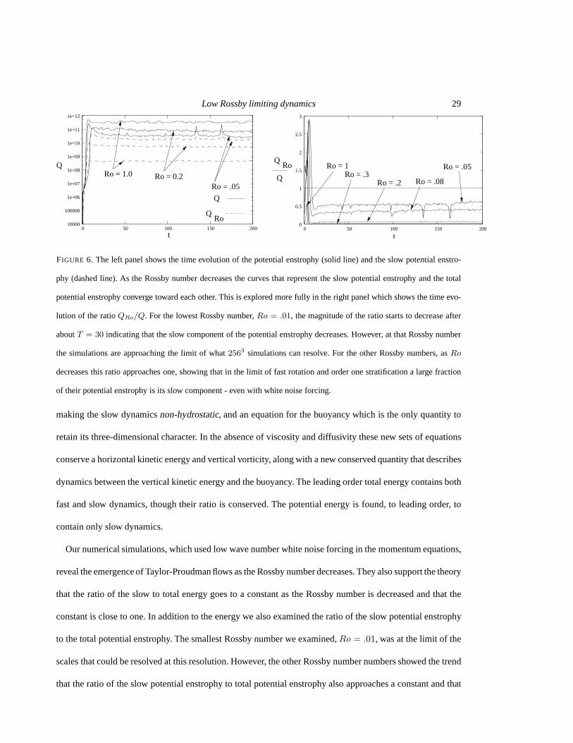
QRo = 1.0 Ro = 0.2

Q

t t

Ro = .2Ro = .3

Ro = 1

Ro = .08

Ro = .05

Q

Q

QRo = .05

Ro

Ro 10000

100000

1e+06

1e+07

1e+08

1e+09

1e+10

1e+11

1e+12

0 50 100 150 200 0

0.5

1

1.5

2

2.5

3

0 50 100 150 200

FIGURE 6. The left panel shows the time evolution of the potential enstrophy (solid line) and the slow potential enstro-

phy (dashed line). As the Rossby number decreases the curvesthat represent the slow potential enstrophy and the total

potential enstrophy converge toward each other. This is explored more fully in the right panel which shows the time evo-

lution of the ratioQRo/Q. For the lowest Rossby number,Ro = .01, the magnitude of the ratio starts to decrease after

aboutT = 30 indicating that the slow component of the potential enstrophy decreases. However, at that Rossby number

the simulations are approaching the limit of what2563 simulations can resolve. For the other Rossby numbers, asRo

decreases this ratio approaches one, showing that in the limit of fast rotation and order one stratification a large fraction

of their potential enstrophy is its slow component - even with white noise forcing.

making the slow dynamicsnon-hydrostatic, and an equation for the buoyancy which is the only quantity to

retain its three-dimensional character. In the absence of viscosity and diffusivity these new sets of equations

conserve a horizontal kinetic energy and vertical vorticity, along with a new conserved quantity that describes

dynamics between the vertical kinetic energy and the buoyancy. The leading order total energy contains both

fast and slow dynamics, though their ratio is conserved. Thepotential energy is found, to leading order, to

contain only slow dynamics.

Our numerical simulations, which used low wave number whitenoise forcing in the momentum equations,

reveal the emergence of Taylor-Proudman flows as the Rossby number decreases. They also support the theory

that the ratio of the slow to total energy goes to a constant asthe Rossby number is decreased and that the

constant is close to one. In addition to the energy we also examined the ratio of the slow potential enstrophy

to the total potential enstrophy. The smallest Rossby number we examined,Ro = .01, was at the limit of the

scales that could be resolved at this resolution. However, the other Rossby number numbers showed the trend

that the ratio of the slow potential enstrophy to total potential enstrophy also approaches a constant and that


constant trends toward one. These numerical simulations indicate that some of the aspects dynamics derived

in this paper exist even in the presence of white noise forcing and hyperviscosity.

Appendix

Analysis of the fast operator

The fast operatorLF is defined on the Hilbert spaceX of 2π-periodic square-integrable vector fieldsu =

(v, ρ) that are divergence free,∇ · v = 0. In the spaceX the eigenfunctions ofLF are given by Fourier

modes of the formuk(x) = eik·xrk wherek = (k, l,m) is the wave number andrk = (vk, ρk) is a

fixed vector. The divergence free condition reduces to the algebraic constraintvk · k = 0. In terms of

the Fourier eigenmodeuk(x) the eigenvalue equationLFuk = λkuk reduces to the algebraic eigenvalue

problemLF (k)rk = λkrk, where the matrix symbolLF (k) is given, fork 6= 0 andk = 0 respectively, by

LF (k) =1

|k|2

−kl −(l2 +m2) 0 0

k2 +m2 kl 0 0

−lm km 0 0

0 0 0 0

, LF (0) =

0 −1 0 0

1 0 0 0

0 0 0 0

0 0 0 0

, (A. 1)

with |k|2 = k2+l2+m2. The algebraic eigenvalue problem has four purely imaginary eigenvalues,λk = iωαk

,

with ω±1k

= ± m|k| corresponding to fast inertial modes and the double eigenvalueω0

k= 0 corresponding to

the slow modes. The associated eigenvectors are given as follows. If |kH | 6= 0 there are three eigenvectors,

r1k =

1√2|kH ||k|

−l|k|+ ikm

k|k|+ ilm

−i|kH |2

0

, r−1k

=1√

2|kH ||k|

l|k| − ikm

−k|k| − ilm

i|kH |2

0

, r0k =

0

0

0

1

. (A. 2)


The fourth eigenvector does not satisfy the incompressibility constraintvk · k = 0. If |kH | = 0 but |k| 6= 0,

thenω±1k

= ±1, ω0k= 0, and there are four eigenvectors,

r1k=

1√2

1

−i

0

0

, r−1k

=1√2

1

i

0

0

, r0k=

0

0

0

1

, r0k=

0

0

1

0

, (A. 3)

but the fourth eigenvector,r0k, violates the incompressibility constraint. Finally, if|k| = 0 then there are

two fast modes associated withω±10

= ±1 and two slow modes associated withω00 = 0, with the four

eigenvectors in Eq. (A. 3) now satisfying the incompressibility constraint. Notice that the eigenfunctions are

normalized and satisfy the symmetry conditionrαk= r

−α−k

, where the bar stands for complex conjugation. For

this reason we require that the amplitudesσαk(t) in Eq. (3.34) satisfy the conditionσα

k= σ−α

−kto ensure that

u(x, t) in Eq. (3.34) is real valued.

Formulas for the interaction coefficients

Here we collect the formulas for the interaction coefficientsB(α′,α′′,α)(k′,k′′,k) ,L(α′,α)

kandD(α′,α)

k, which appear in

Fourier formulation of the limiting fast dynamics equations, Eq. (3.37). The quadratic interaction coefficient

B(α′,α′′,α)(k′,k′′,k) is given by,

B(α′,α′′,α)(k′,k′′,k) =

i

2

[(vα

′

k′ · k′′)rα′′

k′′ + (vα′′

k′′ · k′)rα′

k′

]· rα

k. (A. 4)

With this formula we can verify the claim that the fast limiting dynamics equations for the slow modes is

independent of the fast modes, i.e. that the quadratic interaction coefficients corresponding to “fast + fast→

slow” are zero. Because the formula for the quadratic interaction coefficient in Eq. (A. 4) is invariant under

the permutation ofα′ andα′′, andk′ andk′′, it is sufficient to check thatB(−1,1,0)(k′,k′′,k) is zero. The three-wave

resonance equations for this case is

k′ + k

′′ = k,m′

|k′| −m′′

|k′′| = 0. (A. 5)

There are three cases to consider. First, if|kH | 6= 0 thenr0k

in Eq. (A. 2) is orthogonal tor±1k

in both Eq.

(A. 2) and Eq. (A. 3), andB(−1,1,0)(k′,k′′,k) is zero . Second, if|kH | = 0 but |k| 6= 0 thenr0

kin Eq. (A. 3) coincides

with r0k

in the previous case and the quadratic coefficient is again zero. Finally, if |k| = 0 then thererαk

in


Eq. (A. 3) is eitherr0k

or r0k. In this casek′ = −k

′′ and, by symmetry,r−1−k′ = r1

k′ . Direct calculation then

shows that the third component of(v1k′ · (−k

′))r1k′ + (v1

k′ · k′)r1k′ in Eq. (A. 4) is given by,

(v1k′ · (−k

′))w1k′ + (v1

k′ · k′)w1k′ = i|k′

H |2(v1k′ + v1

k′) · k′

= 2i|k′H |2(−l′|k′|, k′|k′|, 0) · (k′, l′,m′) = 0, (A. 6)

and this implies that the dot product with eitherr0k

or r0k

for the quadratic interaction coefficient in Eq. (A. 4)

is again zero. This proves thatB(−1,1,0)(k′,k′′,k) is always zero.

Next, the linear interaction coefficientL(α′,α)k

in Eq. (3.37) is given by,

L(α′,α)k

= (rαk)∗LS(k)r

α′

k , (A. 7)

where the matrix symbolLS(k) associated with the slow operatorLS is given, fork 6= 0 andk = 0

respectively, by

LS(k) =1

Fr

0 0 0 − km|k|2

0 0 0 − lm|k|2

0 0 0 |kH |2

|k|2

0 0 −1 0

, LS(0) =1

Fr

0 0 0 0

0 0 0 0

0 0 0 1

0 0 −1 0

. (A. 8)

Direct calculation of these coefficients with the eigenvectors given in Eqs. (A. 2) – (A. 3) gives the explicit

values ofL(0,±1)k

= ±i/√2 andL(±1,0)

k= ∓i/

√2 whenk = (k, l, 0), L(0,0)

0= 1, andL(0,0)

0= −1 when

k = 0, and zero otherwise.

Finally, the diffusion coefficientD(α′,α)k

in Eq. (3.37) is given by,

D(α′,α)k

= (rαk)∗D(k)rα

′

k, (A. 9)

whereD(k) is the diagonal matrix

D(k) = diag

(− 1Re |k|2,− 1

Re |k|2,− 1Re |k|2,− 1

RePr |k|2), (A. 10)

and direct calculation with the eigenvectors given in Eqs. (A. 2) – (A. 3) shows that

D(1,1)k

= D(−1,−1)k

= − 1

Re|k|2, D

(0,0)k

= − 1

RePr|k|2, (A. 11)

and zero otherwise.


REFERENCES

AAGAARD , K. & CARMACK , E. C. 1989 The Role of sea ice and other fresh water in the Arctic circulation.Journal of

Geophysical Research94 (C10), 14,485 – 14,498.

BABIN , A., MAHALOV, A., & N ICOLAENKO, B. 1996 Global splitting, integrability and regularity of3D Euler and

Navier-Stokes equations for uniformly rotating fluids.European J. mechanics B/Fluids15 (3), 291–300.

BABIN , A., MAHALOV, A., NICOLAENKO, B. & ZHOU, Y. 1997 On the asymptotic regimes and the strongly stratified

limit of rotating boussinesq equations.Theoretical and Computational Fluid Dynamics9 (3/4), 223 – 51.

BABIN , A., MAHALOV, A.,& N ICOLAENKO 1998 On nonlinear baroclinic waves and adjustment of pancake dynamics.

Theoretical and Computational Fluid Dynamics11 (3/4), 215–235.

BABIN , A., MAHALOV, A., & N ICOLAENKO, B. 2002 Fast singular oscillating limits of stably stratified three-

dimensional Euler and Navier-Stokes equations and ageostrophic fronts, 126–201, inLarge-Scale Atmosphere-

Ocean Dynamics(J. Hunt, J. Norbury, and I. Roulstone, eds.), Cambridge University Press.

CHAPMAN , DAVID C. & HAIDVOGEL , DALE B. 1992 Formation of taylor caps over tall isolated seamountin a stratified

ocean.Geophysical and Astrophysical Fluid Dynamics64, 31–65.

CHARNEY, J. G. 1948 On the scale of atmospheric motions.Geofysiske Publikasjoner17 (2), 3.

CHASNOV, J.R. 1994 Similarity states of passive scalar transport inisotropic turbulence.Phys. Fluids6, 1036–1051.

CHEN, QIAONING , CHEN, SHIYI , EYINK , G. L. & HOLM , D. D. 2005 Resonant interactions in rotating homogeneous

three-dimensional turbulence.Journal of Fluid Mechanics542, 139 – 64.

DAVIDSON, P. A., STAPLEHURST, P. J. & DALZIEL , S. B. 2006 On the evolution of eddies in a rapidly rotating system.

Journal of Fluid Mechanics557, 135 – 144.

DAVIES, P.A. 1972 Experiments on taylor columns in rotating, stratified fluids.Journal of Fluid Mechanics54, 691–718.

EMBID , P. F. & MAJDA, A. J. 1996 Averaging over fast gravity waves for geophysical flows with arbitrary potential

vorticity. Communications in partial differential equations21 (3-4), 619 – 658.

EMBID , P. F. & MAJDA, A. J. 1998 Low Froude number limiting dynamics for stably stratified flow with small or finite

Rossby numbers.Geophysical and astrophysical fluid dynamics87 (1-2), 1 – 50.

EMERY, W. J., LEE, W. G., & MAGAARD , L. 1984 Geographic and Seasonal Distributions of Brunt-Vaisala Frequency

and Rossby Radii in the North Pacific and North Atlantic.Journal of Physical Oceanography14, 294 – 317.

GREENSPAN, H.P. 1990The theory of rotating fluids. Breukelen Press.

HEYWOOD, K. J., GARABATO , A. N. & STEVENS, D. P. 2002 High mixing rates in the abyssal southern ocean.Nature

415, 1011–1014.

HIDE, R. & IBBETSON, A. 1966 An experimental study of taylor columns.Icarus5, 279–290.


HOGG, NELSON G. 1973 On the stratified taylor column.Journal of Fluid Mechanics58, 517–537.

JEFFERY, N. & W INGATE B. 2009 The effect of tilted rotation on shear instabilitiesat low stratifications.Journal of

Physical Oceanography39, 3147–3161.

JONES, E. P., RUDELS, B. & A NDERSON, L. G. 1995 Deep waters of the Arctic Ocean: origins and circulation.Deep-

Sea Research42, 737–760.

KELVIN , LORD W. 1880 Vibrations of a columnar vortex.Philosophy Magazine10, 155 – 168.

KLAINERMAN , S. & MAJDA, A. 1981 Singular limits of quasilinear hyperbolic systemswith large parameters and the

incompressible limit of compressible fluids.Communications on Pure and Applied Math34 (4), 481 – 524.

LAX , P. 2002Functional Analysis. Wiley-Interscience, New York, New York.

LEBLOND, P.H. & MYSAK , L.A. 1978 Waves in the Ocean. Elsevier Oceanography Series 20. Elsevier Scientific

Publishing Company.

MAJDA, A. 1984Compressible Fluid Flow and Systems of Conservation Laws inSeveral Space variables. Springer-

Verlag, New York, New York.

MAJDA, AJ & GROTE, MJ 1997 Model dynamics and vertical collapse in decaying strongly stratified flows.Physics of

fluids9 (10), 2932–2940, times cited: 28.

MAJDA, A. J. & EMBID , P. 1998 Averaging over fast gravity waves for geophysical flows with unbalanced initial data.

Theoretical and Computational Fluid Dynamics11 (3/4), 155 – 69.

MOHN, CHRISTIAN, BARTSCH, JOACHIM & M EINCKE, JENS2002 Observations of the mass and flow field at porcupine

bank.ICES Journal of Marine Science59, 380–392.

OTHEGUY, P., CHOMAZ , J., & BILLANT , P. 2006 Elliptic and zigzag instabilities on co-rotating vertical vortices in a

stratified fluid.Journal of Fluid Mechanics553, 253–272.

POTYLITSIN , P. G. & PELTIER, W. R. 1998 Stratification effects on the stability of columnar vortices on thef -plane.

Journal of Fluid Mechanics355, 45 – 79.

POTYLITSIN , P. G. & PELTIER, W. R. 2003 On the nonlinear evolution of columnar vortices in a rotating environment.

Geophysical and Astrophysical Fluid Dynamics97, 365 – 391.

RILEY, J. J. &DEBRUYNKOPS, S. M. 2003 Dynamics of turbulence strongly influenced by buoyancy.Physics of Fluids

15 (7), 2047 – 59.

RILEY, J. J. & LELONG, M. P. 2000 Fluid motions in the presence of strong stable stratification.Annual Review of Fluid

Mechanics32, 613 – 657.

SCHOCHET, S. 1987 Singular limits in bounded domains for quasilinearsymmetric hyperbolic systems having a vorticity

equation.Journal of Differential Equations68 (3), 400–428.

SCHOCHET, S. 1994 Fast singular limits of hyperbolic pde’s.Journal of Differential Equations114, 476–512.


SMITH , L. M. & WALEFFE, F. 2002 Generation of slow large scales in forced rotating stratified turbulence.Journal of

Fluid Mechanics451, 145 – 68.

SREENIVASAN, B. & DAVIDSON, P. A. 2008 On the formation of cyclones and anticyclones in arotating fluid.Physics

of Fluids20, 085104.

STAPLEHURST, P. J., DAVIDSON, P. A., & DALZIEL , S. B. 2008 Structure formation in homogeneous freely decaying

rotating turbulence.Journal of Fluid Mechanics598, 81 – 105.

TAYLOR , G.I. 1921 Experiments with rotating fluids.Proceedings of the Royal Society of London100, 114–121

TIMMERMANS , M.L. AND MELLING , H. AND RAINVILLE , L. 2007 Dynamics in the deep Canada Basin, Arctic Ocean,

inferred by thermistor-chain time seriesJournal of Physical Oceanography37, 1066 – 1076

TIMMERMANS , M.L. AND RAINVILLE , L. AND THOMAS, L. AND PROSHUTINSKY, A. 2010 Moored observations of

bottom-intensified motions in the deep Canada BasinJournal of Marine Research68, 1, in press

WOODGATE, R., AAGAARD , K., MUENCH, R., GUNN, J., BJORK, G., RUDELS, B., ROACH, A.T., & SCHAUER, U.

2001 The Arctic Ocean Boundary Current along the Eurasian slope and the adjacent Lomonosov Ridge: Water mass

properties, transports and transformations from moored instruments.Deep-Sea Research48, 1757 – 1892.

VAN HAREN, H. AND M ILLOT, C. 2005 Gyroscopic waves in the Mediterranean SeaGeophysical Research Letters32,

24, 1 – 4.

low rossby limiting dynamics for stably stratiﬁed ﬂow with ... · o(1) froude number; after a...

Documents