1

LP-100A

Digital Vector RF Wattmeter

Operations Manual

September 2013 TelePost Incorporated

Rev. G16

Covers LP-100A serial numbers starting at 2020, and firmware beginning at v1.2.3.1

2

Compliance Statements…

Federal Communications Commission Statement (USA)

This device complies with Part 15 of the FCC Rules. Operation is subject to the following two conditions: (1) this device may not cause harmful interference, and (2) this device must accept any interference received, including interference that may cause undesired operation.

European Union Declaration of Conformity

TelePost Inc. declares that the product: Product Name: Digital Vector RF Wattmeter Model Number:LP-100(A) Conforms to the following Product Specifications: EN 55022: 1998 Class B following the provisions of the Electromagnetic Compatibility Directive 89/336/EEC, tested and verified 3-17-2006 at University of Michigan Radiation Laboratory.

Industry Canada Compliance Statement Canada Digital Apparatus EMI Standard This Class B digital apparatus meets all the requirements of the Canadian Interference-Causing Equipment Regulations. Cet appareil numerique de la classe B respecte toutes les exigences du Reglement sur le material brouilleur du Canada.

Copyright and Trademark Disclosures LP-100(A) is a trademark of TelePost Inc. Windows® is a registered trademark of Microsoft Corporation. Teflon® is a registered trademark of E.I. du Pont de Nemours and Company. PICmicro® is a registered trademark of MicroChip Technology Inc. Material in this document copyrighted © 2013 TelePost Inc. All rights reserved. All firmware and software used in the LP-100(A), VCP and Plot programs copyrighted © 2004-2013 TelePost Inc. All rights reserved. MicroCode Loader is a copyrighted program from Mecanique, http://www.mecanique.co.uk/.

3

Table of Contents

Introduction ......................................................................................................... 4

Connections ......................................................................................................... 5 Operation Overview ............................................................................................. 6 Detailed Operation .............................................................................................. 9 Setup Menus ...................................................................................................... 14

Circuit Description ............................................................................................. 16 Schematic .......................................................................................................... 18 Software ........................................................................................................... 20 Specifications .................................................................................................... 26 Warranty ........................................................................................................... 27

Appendix ............................................................................................................ 28 Calibration ......................................................................................................... 31 Note: Calibration info is provided for reference. LP-100A is factory calibrated with NIST traceable instruments.

4

Introduction The LP-100A is designed as an accurate instrument for monitoring station performance. It provides a number of unique features not seen before in a ham radio wattmeter. The most obvious of these is the vector display. This display shows the complex impedance of the load in two ways. The top line of the display shows impedance in polar form… i.e., magnitude and phase of the impedance. The bottom line shows the real and imaginary components of impedance… i.e., R +jX. The parameters are displayed in a range of 0.1 to 999.9 ohms. Phase is displayed in 0.1 degree increments from 0-90 degrees. Features include… Fast, high contrast GVFD display with bargraphs for power and SWR, along with numerical readout for both

Bargraphs customizable for style, decay, behavior and range

Professional dBm / Return Loss display

50 mW to 3000W with three autoranging scales (options for 5 & 10KW)

Power display resolution of 0.01 to 1W depending on scale

Frequency coverage of 1.8-54 MHz, with automatic per-band correction

Z, R, |X| display from 0-999.9 ohms each

Separate coupler with 50 ohm ports for uncluttered desktop

Peak-hold numerical power readout with "hang" characteristic for power and SWR

SWR accuracy < .15 (5%) from about .1W to 3000W, .05 typical

Power accuracy is 3% typical at any rated power level or frequency from 1W to 3000W after calibration, usable to 0.05W

Can be easily matched in the field to external standard to within 0.1% on each band

Power display is Fwd or Net power delivered to the load ( Fwd minus Ref power).

SWR Alarm system with set points for Off, 1.5, 2.0. 2.5, 3.0 and user setting. Includes “snooze” button for tuning, and power threshold.

Windows freeware Virtual Control Panel for software / remote control

Support within TRX-Manager for direct remote monitoring

Advanced automatic charting capability for SWR, RL, Z, R, X , reflection coefficient and Smith Chart

Built-in bootloader to allow for firmware upgrades to be downloaded and installed.

Call sign screen saver to extend life of display, scrolls a full screen call sign across the screen. Call sign is set in Setup screen.

Direct input for bench testing & field strength measurements, -15 to +33 dBm.

Conforms to FCC Part 15 A & B, ICAS and CE radiated emission limits, tested and verified by accredited lab

This manual will address the operation of the LP-100A. For those who are interested, there is also a section on Calibration, even though this is already done at the factory. There is an Appendix with interesting information the user might find useful.

RoHS Statement The EU adopted a set of standards for the “Reduction of Hazardous Substances” in July 2006. LP-100A’s shipped to EU are 100% RoHS compliant in both parts and manufacturing processes. There may be some long term reliability issues associated with RoHS compliant solders and parts, but unlike some industries like aerospace and medical, we are not exempt from these rules. We have seen no indication of reduced performance or longevity.

5

Connections Connections… Power: 11-16 VDC @ 330 mA max., center pin +, 2.5mm ID. The lead with the white stripe on the supplied cable is + PTT: Loop the PTT (amp keying) between your amplifier and rig through the LP-100A using RCA connectors RS-232: Connects to computer… standard M-F straight through DB9 serial cable. See manual for usage. Current/Voltage: Connect to corresponding jacks on the coupler using supplied RG-58U cables.

Note: This guide assumes you are using firmware version 1.2.3.1 or newer.

6

Operation Overview Operation of the LP-100A is straightforward, and designed to require a minimum of input. There are only three buttons which are used in combination to access all the menus on the LP-100A. There are five main modes for the LP-100A, which are accessed by momentarily pressing the “Mode” button. The mode status is saved in non-volatile memory, and the LP-100A will return to the saved mode upon powering up. There is also an automatic three-step screen saver mode which dims the screen after 1 second of inactivity, scrolls your call sign across the screen after a user programmed delay time, and turns the display off after another user programmed delay time. The first step is only active in the Normal (most often used) mode. More on this below.

Mode Button

There are five basic modes, selectable with the Mode button… Normal, Vector, dBm, Field Strength and Peak-to-Average. The mode button is also used to access Setup and Calibrate modes by holding the button for 1 second to access Setup and another 1 second to access Calibration. To return to the normal sequence of mode selections, press Mode button for 1 second from the Calibrate mode. Normal mode is designed to display all the information you normally need on one

screen. It displays power in three auto-ranging scales, and SWR (or Ref Pwr), plus bar graphs for both. A summary of the behavior options for the bargraph and numerical displays is provided below in the Setup section, along with the default settings. There are more details in the manual. For those in a hurry, see the section below on Normal Operation. Vector mode displays magnitude of Z, phase angle of Z, X and R. These values are relative to the “LOAD” connector, not the antenna. There is much more info in the manual on interpreting this screen, as well as using the Plot program to do automatic graphing of a number of parameters. dBm mode uses professional dBm and RL (Return Loss) terminology instead of

watts and SWR to indicate power and load quality. The resolution is 0.1 dB for both. The range is +15 dBm to +64.9 dBm, and RL from 0 to 49.9 dB. Direct/Field Strength mode is similar to dBm mode except that it is calibrated to display power from –15 dBm to +33 dBm. There is no return loss in this mode because it does not utilize the coupler. Power is supplied directly to one of the inputs on the back of the LP-100A. This mode can be used for accurate low power bench measurements, as in checking the output to a transverter or the level of a local oscillator or mixer. It is also very useful for doing antenna field strength measurements, as in plotting a beam pattern. There is more on this in the manual, including the use of VCP (Virtual Control Panel) and a program called PolarPlot to automatically plot antenna patterns. NOTE: The maximum power for the direct inputs is 2W. Peak-to-Average Ratio displays the ratio of the peak signal to average level of the RF envelope. It is used to determine the effectiveness of speech processing and compression equipment in your radio. It requires the use of an audio test tone, available on my website, that I created specifically for this mode. Again, there is more information in the manual. Setup and Calibrate Allows accessing the Setup and Calibrate modes. Hold Mode

button for 1 second to enter Setup mode (top right picture). Hold another second to enter Calibration mode (bottom right picture). Once you are in each of these modes, the Mode button lets you cycle through the choices of that mode. There is more information on the Setup page of this guide. Details for the Calibration mode are in the LP-100A Assembly and Operation manual. Normally, this mode is not used except by kit builders, since the assembled meters are factory calibrated with accuracy traceable to NIST.

7

Operation Overview Cont’d

Alarm (Dn) Button

The Alarm button is used to set the SWR alarm set point. There are 6 choices… OFF, 1.5, 2.0, 2.5, 3.0 & User. The User setting is adjusted in Setup mode, and the programmed value is shown next to the word “User” on the display. Holding the Alarm button wi ll advance the choices every half second or so. Tapping the button will put the Alarm in “snooze” mode for a minute. Tapping again during tuning will reset the function for another minute. The snooze mode allows adjusting an antenna tuner without the alarm going off, but it returns to normal after tuning to protect the amplifier as intended.

Peak/Avg/Tune (Up) Button This button provides two functions. 1) Short Tap (momentary) – Cycles among the three power display modes… Average, Peak Hold and Tune.

----- Power Mode Indicator. W=Average, W=Peak, T=Tune (pulser)

In all cases, the bar graphs remain in fast attack mode, with decay that’s adjustable in Setup. The character after the numerical power readout indicates which mode you are in. A “W” indicates peak mode, a “w” indicates average mode and a “T” indicates tune mode. Average mode is best for taking accurate measurements with steady state signals, or for tuning an antenna tuner. Peak is best for CW or SSB operating. Note: The Peak Mode is VERY fast, and can respond to a lip smack, mic button click, etc. Don’t be alarmed by this… it is normal, and allows the LP-100A to provide an accurate indication of peak power. Unless a lot of compression is used, the peak reading will occasionally be somewhat higher than the indication with a carrier… as much as 30% depending on the ALC attack time in your rig, and power supply regulation of rig or amplifier. Tune mode is similar to Peak mode, except that the peak hold time constant is set to 0.25 sec as opposed to the hold time set in Setup. The Average and Tune modes use the preset bargraph range in the setup section, while the Peak mode shows a fixed 13 dB range. The Tune mode is designed mainly for tuning an amplifier using a pulser, and uses a much longer decay to smooth out the pulses.

Peak/Avg/Tune (Up) Button cont’d 2) Long Tap (1/2 second) - Cycles among the three dual coupler selections… Coupler 1, Coupler 2, Auto-Sense.

The dual coupler option must be installed for the selections to do anything. When in Auto-Sense, the LP-100A will display the data from whichever coupler is receiving the most power. This is especially useful for SO2R operation, or when using a rig with separate HF and 6m outputs. The meter automatically applies the correct calibration table for the active coupler. Coupler models can be intermixed. A little “arrow” next to the “SWR” text indicates which coupler is active (down for coupler 1, up for coupler 2).

8

Operation Overview Cont’d

Normal Operation

The default settings that affect normal operation are supplied set as below… Net/Fwd power… Net Low power range… 15W Mid power range… 100W High power range… 1500W Alarm Pwr Threshold… 0W Alarm Set Point… 2:1 Tuning Range… 12dB Pwr Average samples… 8 SWR Average samples… 2 Peak Hold Time… 2 sec Bargraph Decay… Med Coupler… LPC1 (or other coupler as ordered) SWR Resting Style… - . - - Lower Bargraph Mode… SWR Display Brightness… 6 SS Timers… Scroll=2, Sleep=5 SS Reset… Mode button or RF Power Sensing Optional Mode Display… Optional modes OFF SWR Power Threshold… 0.5W Peak Power Reset Threshold… 50% Dual Coupler Option… Disabled unless you ordered dual couplers

See Setup Mode section for details on setup options. Generally, the LP-100A is left in the Normal mode. For SSB or CW operation, you should use Peak power mode. You can access this mode by tapping the Peak/Avg/Tune button until you see a capital “W” next to the power readout. This mode will show peak power and SWR and hold them for the preset hold time unless a higher peak is detected, at which time the timer resets. Do not use this mode for steady-state power or SWR measurements. The peak power reading can be as much as 30% higher than steady-state power readings taken in the Fast mode. This is because of the ability of the transmitter or amplifier to deliver short bursts of higher power due mainly to power supply regulation issues. This is especially true of older amplifiers with unregulated power supplies, but also is affected by the ALC timing characteristics of modern rigs in both CW and SSB. The peak detector in the LP-100A is very fast, and will grab even the smallest peak. Peak SWR will show values a little higher than steady-state at times due to the wide dynamic range of the LP-100A. There is more about this in the Appendix of the manual. For amplifier tuning with a carrier, you should use the Average mode (small “w”) to see both bargraph and numerical readout change as you tune. You can stay in Peak mode if all you care about is the bargraph. When using a pulser for tuning, switch to Tune mode “capital “T”) for fast update of both bargraph and numerical readout. The bargraph sampling in the LP-100A is about 100 samples/second, and it will display a single dit at 60 wpm, or a string of pulses from a pulser. Full accuracy should be attainable down to about 500 mW for both power and SWR. Good accuracy should still be maintained down to < 100 mW. For antenna tuner adjustment, any mode is good, as both the bargraph and numerical readout update continuously. Use the dBm/RL mode if you prefer peaking rather than dipping. Tapping the Alarm button will temporarily disable the alarm during tuning, then turn it back on after a minute. Normally, the SWR Alarm should be set for 2.0:1 unless you purposely operate with an antenna that is close to 2.0:1 SWR. It is up to you whether to enable the alarm sounder, by using JP1. In any case, it is recommended that you loop your amplifier PTT (keying) through the LP-100A. This helps protect your amplifier.

9

Detailed Operation

Operation of the LP-100A is straightforward, and designed to require a minimum of input once set up and calibrated. There are only three buttons which are used in combination to access all the menus on the LP-100A. There are five main modes for the LP-100A, which are accessed by momentarily pressing the “Mode” button. Pressing the button in mode 4 returns you to mode 1. The mode status is saved in non-volatile memory, and the LP-100A will return to the saved mode upon powering up. There is also an automatic two-step screen saver mode which dims the screen after approx. 30 sec of inactivity, and marches your call sign across the screen after approx. 2 min. of inactivity. This is done to extend the life of the GVFD display.

Mode There are five selectable modes… Normal, Vector, dBm, Field Strength and Compression. A sixth mode which display relative power and phase between phased array elements or stacked beams is in the works as well. Normal mode is designed to display all the information you normally need on one screen. It displays power in three auto-ranging scales, and SWR, plus bar graphs for both. Vector mode displays Z, Phase angle of Z, X and R. These values are relative to the “LOAD” connector, not the antenna. Antenna Z

can be calculated by knowing the feedline length and using a program like TLW, or a Smith Chart. Note: The LP-100A cannot determine the sign of X automatically. dBm mode uses professional dBm and RL (Return Loss) instead of watts and SWR to indicate power and load quality. The resolution

is 0.1 dB for both. The range is +15 dBm to +64 dBm, and RL from 0 to 49.9 dB. Direct/Field Strength mode is similar to dBm mode except that it is calibrated to display power from –15 dBm to +33 dBm. There is no return loss in this mode because it does not utilize the coupler. Power is supplied directly to one of the inputs on the back of the LP-100A. This mode can be used for accurate low power bench measurements, as in checking the output to a transverter or the level of a local oscillator of mixer. It is also very useful for doing antenna field strength measurements, as in checking a beam pattern. This requires feeding a small pickup antenna to one of the inputs. The LP-100A could be set up in a field, connected to a laptop computer with wi-fi, and the results can be read over the wireless LAN back in the shack. This eliminates any wiring that could distort the pattern. NOTE: The maximum power for the direct inputs is 2W.

Peak-to-Average Ratio displays the ratio of the peak signal to average level of the RF envelope. It is used to determine the effectiveness of speech processing and compression equipment in your radio. Alarm

The Alarm button is used to set the SWR alarm set point. There are 6 choices… OFF, 1.5, 2.0, 2.5, 3.0 & User. The User setting is adjusted in Setup/CAL mode, and the programmed value is shown next to the word “User” on the display. Holding the Alarm button will advance the choices every half second or so. Tapping the button will put the Alarm in “snooze” mode for a minute. Tapping again during tuning will reset the function for another minute. This allows adjusting an antenna tuner without the alarm going off, but it returns to normal after tuning to protect the amplifier as intended. If “Avg. During Snooze” is selected for the W Mode SWR Display setting, then entering Snooze mode will also make the SWR display average instead of peak until the timer times out. This makes antenna tuning easier since you can stay in the W mode even during antenna tuning.

10

Detailed Operation Cont’d

Peak/Avg/Tune

This button toggles between a pseudo-average numerical display, a peak-hold display and a tune mode. In all cases, the bar graphs remain in fast mode. The character after the numerical power readout indicates which mode you are in. A “W” indicates peak mode, a “w” indicates average mode and a “T” indicates tune mode. Average mode is best for taking accurate measurements with steady state signals, or for tuning an antenna tuner. Peak is best for CW or SSB operating. Note: The Peak Mode is VERY fast, and can respond to a lip smack, mic button click, etc. Don’t be alarmed by this… it is normal, and allows the LP-100A to provide an accurate indication of peak power. Unless a lot of compression is used, the peak reading will usually be somewhat higher than the indication with a carrier… as much as 30% depending on the ALC attack time in your rig, and power supply regulation of rig and amplifier. Tune mode is similar to Peak mode, except that the peak hold time constant is set to 0.25 sec as opposed to the hold time set in Setup. The Average and Tune modes use the preset bargraph range in the setup section, while the Peak mode shows a fixed 13 dB range. The Tune mode is designed mainly for tuning an amplifier using a pulser. The button also allows selection of couplers if the Dual Coupler Option is installed. Holding the button for a second will display and advance the coupler choice. Choices are “Channel 1”, Channel 2”, “AutoSense”. Press/hold once for each change. A small arrow next to the SWR title indicates which coupler is active. A down arrow indicates CH1, and up arrow CH2.

Setup The Setup/Calibration modes can be accessed with the Mode button. To enter Setup mode, press and hold Mode button for about 1 second. Once in Setup mode, the Mode button is used to cycle through the setup screens. If you hold the button too long, you will advance to the Calibrate mode. Simply hold the button again to return to the main screen and start over. Reference. This screen display the reference voltage from the gain/phase detector, the RSSI output from the counter AGC amplifier and temperature in degrees F & C. It is only mainly for diagnostics. Pressing the Alarm button in this mode resets the PIC, quite useful when flash programming the PIC. The reset does not affect setup/calibration settings. Pressing the Peak/Avg/Tune button toggles the Temp display between degrees C and F. User Alarm Setting. Allows setting a user threshold other than the preset choices. Any setting from 1.0 to 5.0 is permissible.

AL Thresh/Pwr Mode. Allows selection of a power threshold for the SWR alarm. The normal setting is zero, meaning that the alarm will work at any power level. Choices are 0, 0.1, 1.0, 10.0, 100.0W. This is useful for multi-transmitter contest setups where significant energy from a nearby antenna might be present on the output of the LP-100A coupler. If the energy is from another band, the LP-100A will display SWR, which will be high. By setting a power threshold for the alarm, it will keep the alarm from tripping on induced power. The Pwr Mode allows selection of Net or Fwd power. Net is Fwd minus Ref… or delivered power. F+R is the total incident power (including Ref) as displayed on typical wattmeters like a Bird 43. Range. Sets the maximum excursion of the bargraph for the three automatically selected ranges. The choices are… Low – 5, 10, 15, 20, 25W Mid – 50, 75, 100, 125, 150, 175, 200, 225, 250W High – 500, 750, 1000, 1250, 1500, 1750, 2000, 2250, 2500, 3000W Defaults are 15W, 100W and 1500W. Each range allows 10% overhead, so that the 100W selection would extend to 110W, for example. Note: These settings do not affect the numerical readout, which has no limits of any kind. The Dn button selects the range, and the Up button sets the power level, with wraparound to the beginning values.

Bargraph Tuning Range. Sets the width of the bargraph in Average and Tune modes from 3dB to 12dB. This allows tailoring of the bargraph resolution for amplifier tuning to simulate an analog meter. The response is still logarithmic to minimize jitter, and be more like the typical square law analog meter response. The default is 12dB. You can use a narrower range to increase bargraph resolution for amplifier tuning. The default setting of 12dB gives almost 1% bargraph resolution, and the other choices give much better than 1% resolution. Averaging Samples. Sets the number of samples for power averaging, adjustable from 2 to 24 samples. Default is 8 samples. Peak Hold Time. Sets the hold time in Peak mode. Adjustable from 0.25 to 5 seconds. The default setting is 2 seconds for normal SSB or CW operation.

11

Detailed Operation Cont’d

Bargraph Decay. Allows setting the decay time of the power bargraph. The default setting is Fast, and provides a decay of less than

one second. The longest setting is Slow, and provides about a 3 second decay. In all cases, the attack is instantaneous.

Coupler Type. This screen is used to select different maximum power values to be used with custom high power couplers. Use Dn/Up to cycle through the choices. The default is LPC1 (the standard coupler). Current choices are “LPC1 3KW 1.8-54MHz, “LPC2 5KW 1.8-30MHz”, “LPC3 250W 0.1 - 20MHz”, ”, “LPC4 5KW 1.8-54MHz”, “LPC5 10KW 1.8-30MHz” and “LPC6 1KW 0.10 to 10MHz”. Use Dn/Up to cycle through choices. SWR Resting Style. This screen is used to select the way you want SWR displayed when you are not transmitting. The choices are… “-.--“, “1.00”, “. . . .”, blank and hold last SWR reading. If you select Hold Last, it will be reset when you transmit again. Use Dn/Up to cycle through choices. Lower Bargrph Mode. This screen is used to select what parameter is displayed on the lower half of the display. The choices are SWR and Reflected Power. If you select Reflected Power, remember that the reflected power will be referenced to either NET power or Forward Power (F+R) depending on your earlier selection for the power display. F+R is the preferred choice to use with REF pwr. Use Dn/Up to select. Callsign Entry. This screen is used to program your callsign into the screen saver. The Dn button is used to select the position of the letter you want to change… 1 thru 6 from left to right. The Up button is used to scroll through the choices… 0 thru 9, A thru Z, space, / and -. Both buttons wrap around. Step thru the positions, scrolling to the letter you want for each position. The callsign is saved as you see it. Display Brightness. This screen is used set the display brightness. Each step represents a 12.5% change in brightness. The default

setting is 6, which equals a brightness level of 75%. This provides almost full brightness, and provides some measure of added display life. You can use any brightness level you like. The display is rated for 50,000 hours (5.7 years) of continuous display at full brightness before brightness drops to half. With the LP-100A’s screen savers, you can expect much more than that with typical operating habits. Use Dn to reduce brightness, Up to increase. The brightness of the screen changes as you adjust it. Screen Save Timers. This screen is used set the display screen savers. The two timers that can be set are the Scroll timer and the Sleep timer. The Scroll timer sets the time in minutes from the last transmission to the time when your call sign starts scrolling across the screen. The Sleep timer sets the time from the last transmission to the time when the display turns off. The Scroll saver should be set first, since it also affects the Sleep timeout. Each can be adjusted for up to 10 minutes (20 minutes total). The screen saver extends display life, and reduces power consumption and heat when the meter is idle. There is also a third screen saver timer, but it is factory preset. It dims the screen to 25% one second after transmission ends when in the Main Mode. If Peak power mode is selected and the hold time is set for 1 second or more, it dims at the end of the hold period. Calibration Calibration Initial Screen. This screen simply identifies that you are in the Calibration mode. Serial Number. All LP-100As after serial #100 are supplied with RG-58U connecting cables between the coupler and main chassis. Earlier versions used RG-174U. This screen allows selection of the appropriate cable. It selects the proper correction table for the cable loss vs. frequency. On later versions, this screen name was changed to Serial Number to compensate for other hardware changes as well as cable type. Gain Zero Trim. This screen allows band-by-band calibration of the balance of the gain detector. The process simply requires a good

quality dummy load. The Dn/Up buttons are adjusted until the resistance on the screen matches the resistance of your dummy load. The LP-100A automatically saves the Cal constants for each band, indexed to frequency. The built-in frequency counter automatically determines the frequency. Phase Zero Trim. This screen allows band-by-band calibration of the balance of the phase detector. The Dn/Up buttons are adjusted until the phase on the screen reads zero degrees. The LP-100A automatically saves the Cal constants for each band, indexed to frequency. The built-in frequency counter automatically determines the frequency. Gain Slope Trim. Allows setting the slope of the magnitude for proper Z at a value removed from 50 ohms. This can be done with any reasonable known load in the 25 or 75-100 ohm range. I am also working on a calibrator kit to simplify this. Phase Slope Trim. Allows calibrating the phase detector. This requires a delay line of known value. In its simplest form, this can be

done by calculating the electrical length of an existing piece of coax in the 3-10’ range, and matching the readout to the calculated length at the frequency used for the calculation. More on this in the Calibration section. I am also working on a calibrator kit to simplify this.

12

Detailed Operation Cont’d

Offset Trim. Provides for calibrating the low level ADC converter accuracy. The screen shows the output voltage of the detector, and the Trim level is set by adjusting for zero voltage with no RF power applied.

Hi/Lo Trim. This screen allows the matching of the direct and divided inputs to the ADC to account for any slight variations in the precision divider.

Master Trim. Adjusts the overall gain for power readout for all frequencies. Fine Trim. Adjusts gain by band for power readout, indexed by frequency. Frequency is determined automatically by a built-in frequency

counter.

Counter Calibration. Allows synchronizing the LP-100A clock with an external reference. Normal Operation

In normal operation, the LP-100A is left in the Normal mode. You’ll notice that the screen dims to 25% one second after powering up or when transmission ends. If Peak power mode is selected and the hold time is set for 1 second or more, it dims at the end of the hold period. This is part of the screen saver, and is designed to maximize display life. All other modes provide full brightness as preset in Setup, since they are not used nearly as much as the Normal mode. For SSB or CW operation, you should use the Peak mode. This mode will show peak power and SWR and hold them for the preset hold time unless a higher peak is detected, at which time the timer resets. Both the numerical value is held, plus a “sticky bar” in the bargraph. This lets you see your maximum peak, but still allows the bargraph to follow your transmitted power at very high speed. Do not use this mode for steady-state power or SWR measurements, as it will be affected by momentary power fluctuations that many modern rigs have.

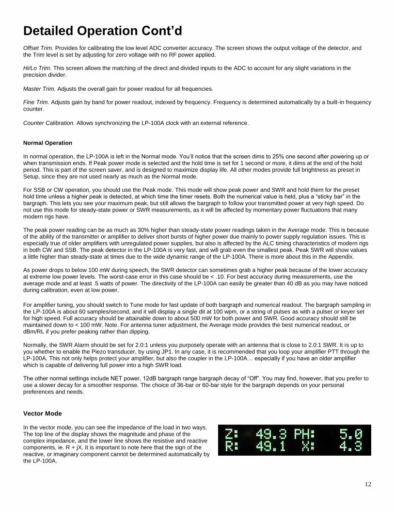
The peak power reading can be as much as 30% higher than steady-state power readings taken in the Average mode. This is because of the ability of the transmitter or amplifier to deliver short bursts of higher power due mainly to power supply regulation issues. This is especially true of older amplifiers with unregulated power supplies, but also is affected by the ALC timing characteristics of modern rigs in both CW and SSB. The peak detector in the LP-100A is very fast, and will grab even the smallest peak. Peak SWR will show values a little higher than steady-state at times due to the wide dynamic range of the LP-100A. There is more about this in the Appendix. As power drops to below 100 mW during speech, the SWR detector can sometimes grab a higher peak because of the lower accuracy at extreme low power levels. The worst-case error in this case should be < .10. For best accuracy during measurements, use the average mode and at least .5 watts of power. The directivity of the LP-100A can easily be greater than 40 dB as you may have noticed during calibration, even at low power. For amplifier tuning, you should switch to Tune mode for fast update of both bargraph and numerical readout. The bargraph sampling in the LP-100A is about 60 samples/second, and it will display a single dit at 100 wpm, or a string of pulses as with a pulser or keyer set for high speed. Full accuracy should be attainable down to about 500 mW for both power and SWR. Good accuracy should still be maintained down to < 100 mW. Note. For antenna tuner adjustment, the Average mode provides the best numerical readout, or dBm/RL if you prefer peaking rather than dipping. Normally, the SWR Alarm should be set for 2.0:1 unless you purposely operate with an antenna that is close to 2.0:1 SWR. It is up to you whether to enable the Piezo transducer, by using JP1. In any case, it is recommended that you loop your amplifier PTT through the LP-100A. This not only helps protect your amplifier, but also the coupler in the LP-100A… especially if you have an older amplifier which is capable of delivering full power into a high SWR load. The other normal settings include NET power, 12dB bargraph range bargraph decay of “Off”. You may find, however, that you prefer to use a slower decay for a smoother response. The choice of 36-bar or 60-bar style for the bargraph depends on your personal preferences and needs. Vector Mode In the vector mode, you can see the impedance of the load in two ways. The top line of the display shows the magnitude and phase of the complex impedance, and the lower line shows the resistive and reactive components, ie. R + jX. It is important to note here that the sign of the reactive, or imaginary component cannot be determined automatically by the LP-100A.

13

Detailed Operation Cont’d

If you QSY up from your current frequency, and the reactance goes up, then the reactance is inductive (sign is “+”), and conversely if it goes down, then the reactance is capacitive (sign is “-“). A suitable distance is QSY is about 100 kHz or more. The LP-Plot program has the ability to determine sign automatically, since it can control your transmitter’s frequency. When it plots a range of frequencies, it uses the slope of the reactance curve to determine sign, and plots the results accordingly. It is important to remember that the impedance displayed on the screen is referenced to the coupler LOAD port. This value is related to actual feedpoint impedance of the antenna by factors relating to the characteristic Z of the line, line length and loss. I plan to add the ability to display actual antenna feedpoint Z into the LP-100A VCP and Plot programs by providing input boxes for feedline type and length. A simple way to provide reasonably accurate antenna Z on the LP-100A display would be to use a feedline which is a multiple of ½ wavelength in electrical length. There would still be some residual error due to feedline loss, but it would give a better representation of feedpoint Z. I am considering adding a CAL screen to allow selection of feedline loss to compensate for this, and I may also allow the future entry of feedline length and Zo data. There will be more info on this and other Impedance related subjects in the upcoming Appendix A. dBm/RL Mode Displays power in dBm from +15 to +64 dBm, and load integrity in dB of return loss from 0 to 49.9 dB. Direct Input/Field Strength Mode

Similar to dBm mode except that it is calibrated to display power from –15 dBm to +33 dBm. There is no return loss in this mode because it does not utilize the coupler. Power is supplied directly to either one of the inputs on the back of the LP-100A. This mode can be used for accurate low power bench measurements, as in checking the output to a transverter or the level of a local oscillator or mixer. It is also very useful for doing antenna field strength measurements, as in checking a beam pattern. This requires feeding a small pickup antenna to one of the inputs. Selecting this mode automatically returns the Peak/Avg/Tune mode to Average. NOTE: The maximum power for the direct inputs is 2W.

Peak-to-Average Mode This mode lets you determine the average power in a signal by taking 40,000 samples/second, and compares this to the peak power in the signal. The result is displayed as a ratio in dB. I provide a couple test tones, which are available on my website at http://www.telepostinc.com/Files/two-level-tone-loop3.zip and http://www.telepostinc.com/Files/loud_tone.zip. The loud tone is used to set the maximum power and proper ALC range (with processing OFF). The two-level tone is used to determine the peak-to-average ratio of the output signal. It can be played back on your PC, or converted to mp3 and played on a portable player. It can be played over a speaker into the microphone, or directly into the mic input. The two-level tone provides alternating loud and soft tones with 20 dB difference in level. This tone should provide the following Peak-to-Average ratios vs. effective compression ratio.

Compression Ratio Peak-to-Average Ratio

0dB 5.2dB

5dB 5.6dB

10dB 3.6dB

15dB 2.2dB

20dB 0dB

I plan more test tones with different characteristics in the future, which is why I decided to keep the display as Peak-to-Average as opposed to Compression, which would only be accurate with one test signal. I will provide additional tables such as the one above with the additional test signals.

14

Setup Menus The Setup mode is accessed by pressing and holding the Mode button for about 1 second until you see the Reference screen shown below. Exiting the Setup mode is done by holding the Mode button for about 2 seconds until you see the Main operating screen. You will pass through the Calibration mode on the way back to Operate.

Reference screen. Displays the reference voltage from the gain/phase detector, as well as the RSSI voltage (Received Signal Strength Indicator) from the AGC chip used in the frequency counter preamp. The screen also shows temperature in Deg F & C. The Dn button resets the microprocessor, and is useful when flash updating the firmware in the LP-100A. The Up button toggles the temperature mode.

This screen is used to set the “User” SWR Alarm setpoint. It can be set between 1.0 and 5.0 in steps of 0.1. Use Dn to lower value, Up to increase it.

This screen allows setting the SWR Alarm power threshold and Power display type. The alarm threshold is used mainly in contesting stations with multiple transmitters to prevent false alarms when energy from another transmitter is picked up by an antenna. The choices are 0,0.1, 1.0 and 10.0 W. The default setting is 0.0W (active at all power levels). The Dn button will allow you to cycle through these choices. Note: This threshold only affects the alarm. Use the SWR threshold Setup screen to limit both the SWR display and alarm below the selected power level. Pwr Mode options are Fwd Power and Net Power (Fwd minus Ref). The Up button toggles these choices. The default is Net.

Range. Allows setting of maximum bargraph scale for the three autoranging scales. The Dn button cycles between Low, Mid & High range. Select a power range, and then set the bargraph maximum range. Bargraph Max Range. The Up button scrolls through the various max power options for each range… Low – 5, 10, 15, 20, 25W … Mid – 50, 75, 100, 125, 150, 175, 200, 225, 250W…High – 500, 750, 1000, 1250, 1500, 1750, 2000, 2250, 2500, 3000W. The displayed range includes 10% above the indicated value. Note: Defaults are 15W, 100W, and 1500W. Note: These ranges are scaled by a factor of x1.67 when using a 5KW coupler, and 3.33 when using a 10KW coupler.

This screen is used to set the width of the bargraph in the Average and Tune modes. The Peak mode is always 13dB. It is useful for optimizing the bargraph resolution for amplifier tuning, for instance. The displayed range goes from the maximum set in the previous screen, to a minimum which is the selected number of dB below that maximum. Default is 12dB Use Dn to lower value, Up to increase it.

This screen allows setting of the number of samples used to average the numerical readout in Average Power mode, and for SWR in all modes. The range is 2 to 24 samples for Power, and 0 to 5 samples for SWR. The default is 8 samples for Power and 2 samples for SWR. Use Dn to cycle through Power settings and Up to cycle through SWR settings. Both wraparound to the beginning.

This screen allows setting the peak hold time in the Peak mode. The range is 0.25 to 5 seconds. The default of 2 seconds is good for normal SSB or CW operation. Use Dn to lower value, Up to increase it.

This screen is used to set the decay rate for the bargraphs. Decay choices are “Fast”, “Med.” and “Slow. The slowest setting corresponds to a decay of about 3 seconds, and smoothes the response considerably for SSB. Default is Med. Try all the settings to see what suits you. Use Dn to lower value, Up to increase it. Note: the attack setting is always fast, and will provide full response to a single dit at 100wpm.

This screen is used to select different maximum power values to be used with custom high power couplers. Use Dn/Up to cycle through the choices. The default is LPC1 (the standard coupler). Current choices are “LPC1 3KW 1.8-54MHz, “LPC2 5KW 1.8-30MHz”, “LPC3 250W 0.1 - 20MHz”, ”, “LPC4 5KW 1.8-54MHz”, “LPC5 10KW 1.8-30MHz” and “LPC6 1KW 0.10 to 10MHz”. Use Dn/Up to cycle through choices.

This screen is used to select the way you want SWR displayed when you are not transmitting. The choices are… “-.--“, “1.00”, “. . . .”, blank and hold last SWR reading. If you select Hold Last, it will be reset when you transmit again. Use Dn/Up to cycle through choices. Default is as shown.

15

Setup Menus Cont’d

This screen is used to select what parameter is displayed on the lower half of the display. The choices are SWR and Reflected Power. If you select Reflected Power, remember that the reflected power will be referenced to either NET power or Forward Power (F+R) depending on your earlier selection for the power display. F+R is the preferred choice to use with REF pwr. Use Dn/Up to select.

This screen is used to program your callsign into the screen saver. The Dn button is used to select the position of the letter you want to change… 1 thru 6 from left to right. The Up button is used to scroll through the choices… 0 thru 9, A thru Z, space, / and -. Both buttons wrap around. Step thru the positions, scrolling to the letter you want for each position. The callsign is saved as you see it.

This screen is used set the display brightness. Each step represents a 12.5% change in brightness. The default setting is 6, which equals a brightness level of 75%. This provides almost full brightness, and provides some measure of added display life. You can use any brightness level you like. The display is rated for 50,000 hours (5.7 years) of continuous display at full brightness before brightness drops to half. With the LP-100A’s screen savers, you can expect much more than that with typical operating habits. Use Dn to reduce brightness, Up to increase. The brightness of the screen changes as you adjust it.

This screen is used set the display screen savers. The two timers that can be set are the Scroll timer and the Sleep timer. The Scroll timer sets the time in minutes from the last transmission to the time when your call sign starts scrolling across the screen. The Sleep timer sets the time from the last transmission to the time when the display turns off. The Scroll saver should be set first, since it also affects the Sleep timeout. Each can be adjusted for up to 10 minutes (20 minutes total). The screen saver extends display life, and reduces power consumption and heat when the meter is idle. There is also a third screen saver timer, but it is factory preset. It dims the screen to 25% one second after transmission ends when in the Main Mode. If Peak power mode is selected and the hold time is set for 1 second or more, it dims at the end of the hold period. The default is as shown.

This screen is used to determine how the meter is waked from ScreenSaver or Sleep modes. The options are… Mode Button or RD Sense, Mode Button Only. The second option is useful in industrial installations where it operation is 24/7 coninuous, and protects the display from excessive wear when the meter is monitored remotely. The default is as shown.

Allows disabling of modes that the user may not use or doesn’t want to scroll through. The optional modes are… dBm/RL, Direct Input (Field Strength) and Peak to Average Ratio. The default is all ON.

Sets the lower limit that the meter will display. The choices are… 0.05W, 0.5W, 2.0W, 5.0W,10.0W. Setting the value higher allows the meter to ignore samples taken during voice pauses. This eliminates some samples taken at the limit of the gain/phase detector accuracy, where SWR readings my be slightly higher. It smooths out the SWR display, and lets SWR adjustments be made while talking, for instance.

This screen sets how far below a peak reading that power must drop before the peak hold timer resets and grabs a new sample. The default is 10%.

This screen allows enabling or disabling of the dual coupler option. This is done so that most users don’t have to see the up/down arrows that show which coupler is active. The choices are “Installed” and “Not Installed”.

16

Circuit Description

Screen Saver

The screen saver works a little differently than it did in the LP-100A due to the different requirements of the GVFD display. It is a three-step process. The first step only works in the Normal mode, while the other two work in all modes and screens. Step 1 is to dim the display to 25% when in Normal mode. Transmitting, even just a dit, will restore full brightness as preset in the Setup screen. One second after transmission it returns to 25%, unless you are in the Peak Hold mode. If you have the hold time set to 1 second or longer, the screen will dim at the end of the hold time for a smoother look. Step 2 scrolls a dimmed, full screen version of your callsign across the display after a preset amount time that you set in Setup (1-10 minutes of inactivity). Step 3 is a “sleep” mode which turns the filaments to the GVFD display off to reduce current draw after a preset amount of time that you set in Setup (1-10 minutes of additional inactivity beyond the scrolling callsign). Transmitting will cancel all three steps. Tapping the Mode button will cancel the second two steps. If you are in the sleep mode, the display will “fade” up as the filaments warm, as opposed to popping back up.

The LP-100A is unique in it’s design in several regards. Refer to the following block diagram during this discussion.

First, instead of using a coupler that produces forward and reflected voltage signals, the LP-100A uses a pair of transformers that sample current in the transmission line and voltage across the load. The samples are split into two paths, which provide signals to both the gain/phase comparator and the power detector. With a 50 ohm non-reactive load, the levels of these two signals will be virtually identical, and the phase between them will be zero degrees. As the load varies from perfect, the relative magnitude and phase of the two samples varies, providing the meter with the information it needs to calculate the complex reflection coefficient, rho, from which SWR and impedance are derived. The combiner adds these two samples vectorially, providing a maximum output of 2x the input power with a perfect load, and proportionately less with less perfect loads. The power sample is rectified in the Schottky diode detector, which uses a special dual diode package to eliminate errors associated with temperature tracking and forward / reverse voltage drop differences. The output of the detector is fed through precision voltage dividers to produce two power ranges, and in combination with a 12-bit A/D converter and precision 2.5V reference chip, provides an effective resolution 12 to 13.6 bits (higher resolution on the lower range). The power sample also feeds an AGC amp which provides a constant, clean sine-wave output signal over a 50dB+ range of input power. This signal is sliced to create a square wave which feeds the frequency counter in the PIC to allow automatic frequency detection at all power levels. This allows for automatic per-band calibration of all calibration parameters in the LP-100A. The AGC amp also provides a DC “Received Signal Strength Indicator” which is used for a number of level detection tasks within the PIC. The A/D converter also receives temperature information from the temp sensor to compensate for any residual temperature related effects in the power detection circuitry.

17

Circuit Description Cont’d

The combiner also provides isolated signals to the gain/phase detector, providing 50dB of isolation between the signals, so that they can be accurately sampled at the input of the gain/phase comparator without affecting each other. The gain/phase comparator produces a DC voltage which is proportional to the log of the magnitude difference between its inputs, and another which is proportional to the phase difference between the inputs. (The sign of phase is not attainable using the present gain/phase detector, but is relatively easy to determine in operation by QSYing up a little and noting the direction of phase movement. I have developed a circuit for sign detection, but it would require a rather substantial change to the PCB. I may change to it in the future, but it wouldn’t be for quite awhile). The phase/gain detector voltages are sampled by the A/D converter and the result is sent to the PIC over a Serial Peripheral Interface. Remaining connections to the PIC include switch inputs for the three front panel switches, interfacing to the GVFD display processor and an SWR alarm relay which is used to kill the PTT to your amplifier to protect both the antenna and amplifier. The SWR alarm also lights a front panel LED, and optionally can be jumpered to sound a piezo transducer. The PIC uses all these signals to calculate all the various displayed parameters. Finally, the PIC provides a standard RS-232 serial interface for remote control and monitoring of the LP-100A. Functions of the LP-100A can be controlled from a Windows® “Virtual Control Panel” program, either locally or over a network connection, including the internet. The PIC’s firmware can also be updated through downloadable hex files which can be “flashed” into the PIC’s memory. A program entitled MicroCode Loader (MCLoader), from Mecanique®, is provided to do this. A Windows® charting program is also provided to allow graphing of any of the LP-100A’s parameters including Z, R, X, SWR and phase angle vs. frequency. The Plot program also offers a Smith Chart display, and I plan to add a translation function to allow for automatic transformation of coupler load Z to antenna feedpoint Z. The programs will provide for inputting feedline length and type for popular types of feedline. More on this is Appendix A.

18

Schematic Page 1

19

Schematic Page 2

Coupler Schematic

20

Software

Connecting to the computer The LP-100A provides a RS-232 serial port. The serial settings are 115,200 baud, 8 bits, no parity, 1 stop bit. The required cable is a straight through (not crossover or null modem), with a male DB9 at one end and a female DB9 at the other. With typical motherboard or bus card provided serial ports, there are no settings required in the computer or driver, just in the application which controls the LP-100A. In the case of the provided software such VCP and Plot, these settings are automatic except for com port selection. Any free com port from 1-15 is acceptable. If your computer doesn’t have a serial port, which is becoming increasingly the case, there is a simple solution as long as the computer has a USB port, which is usually the case. A number of USB to serial adapters are available on the web or at computer/appliance stores. The LP-100A has been successfully used with a number of these. I can personally vouch for the Keyspan USA-19HS, although I don’t know if they have a driver yet for the 64-bit version of Microsoft Vista. An inexpensive converter that some have reported good results with is the Y-105 from ByteRunner, www.byterunner.com. They cost $8.69 plus shipping as of this date, and provide full handshaking (not needed for LP-100A, but useful for some rigs and devices), but no obvious Vista support. This adapter uses the Prolific chipset, which may not be supported in the future. You may need to download a different driver than the one supplied with this unit when using XP. Search the internet for ICUSB232. ByteRunner also sells an adapter which uses the well supported FTDI chipset for about $18, model USB-COM-CBL. Drivers for almost any platform should be downloadable from FTDI. I have been asked about a USB port for the LP-100A, and it would be easy to do, but since all ham software has native RS-232 com support, and older machines don’t have USB ports, I think a RS-232 port with an inexpensive USB adapter where needed is the most flexible choice. The LP-100A has been used successfully over the Internet using serial device servers such as those offered by Lantronix and Digi. I have personally used several of the Lantronix models with no problems.

Virtual Control Panel (VCP) VCP is provided for computer or remote operation of your LP-100A wattmeter. VCP allows you to control the basic functions of the LP-100A, and it also

allows you to monitor the LP-100A parameters remotely.

There are three views for the VCP, selectable under the Style pulldown. The two shown above, plus one which shows all but the setup info. The Menu choices provide the following functionality… Style: Selects among the three views mentioned above Upgrade: Launches the MCLoader program. This program can also be launched manually by adding a shortcut to the program. Help: A work in progress.

The setup controls include Com port selection, callsign entry and a polling rate slider, adjustable from 50 msec to 5 sec. The normal setting is 80 msec, which gives an update rate of 12 samples per second. On slower computers, or over the internet, you can use a slower rate.

21

Software Cont’d

The buttons on the VCP perform the following functions… * Range: Allows switching the maximum power range of the display. Choices are 25, 250, 2500W and Auto for autoranging. * Alarm: Sets the SWR Alarm set point. Choices are Off,1.5,2.0,2.5,3.0. If the alarm on the LP-100A trips, the Alarm button turns red. * Peak/Avg/Tune: Switches between normal and peak-hold modes. The current mode is displayed under the power reading. There are two other versions coming for use with TRX-Manager. The first, called LP-100A VCP Slave, allows the LP-100A to broadcast its data to TRX-Manager for display inside TRX-Manager, either locally or over the internet. The other, LP-100A VCP Master, allows the LP-100A to use TRX-Manager’s remote telnet facility to make a remote connection between the LP-100A and the VCP. In addition to the LP-100A VCP, you can communicate with the LP-100A with a terminal program or your own software using the following commands… A Increments Alarm Set Point selection M Increments Mode selection F Toggles Power Peak/Avg/Tune selection P Poll for data. Example of response… ;1457.00,49.3,005.0,2,N8LP ,0,2,61.6,1.02 From left to right, the comma separated values represent… Power, Z, Phase, SWR Alarm Set Point: 0=off, 1=1.5, 2=2.0, 3=2.5, 4=3.0, Callsign (6 digits with space padding), Power range: 0=High, 1=Mid, 2=Low, Peak Hold Mode: 0=Average, 1= Peak Hold, dBm, SWR Note: The commands for firmware version 1.2.0.0 and above are different than those for earlier versions. I have added an option in the Setup section of VCP, Plot and TRX-Slave to allow use with versions of firmware that are earlier or later than 1.2.0.0. If you need to see the old protocol, or have developed software to work with the LP-100A, you should refer to an older manual to see the differences. The serial settings are 115,200 baud, 8 bits, no parity, 1 stop bit. NOTE: Firmware versions before 1.2.0.0 used a baud rate of 38,400, and before 1.0.3 used a baud rate of 19,200 and did not report dBm or SWR values.

MicroCode Loader Before attempting to flash new firmware, make sure the connection between the LP-100A and PC is solid. You can do this by running the VCP program. MicroCode Loader works with the MCLoader bootstrap loader program installed on your PIC. It allows the user to easily update the firmware in the LP-100A. The correct settings for MicroCode Loader, found under the Options pulldown, are as shown. NOTE: Make sure you settings match these before starting. If you select Program Data, the factory defaults will be loaded into your CAL constant table. All that is required is to download the latest version of the firmware from my website, save it to a convenient folder, such as C:\Program Files\LP-100A-VCP\Updates and then load the file into MCLoader using the File>Open menu. Note: It is important to open the file you want each time you launch MCLoader, or else it will start up with the last used file, and you may forget to open a new file and reprogram your LP-100A with an older version. It is even possible that you might have a file from another device loaded, since MCLoader is used by other manufacturers as well. Once MCLoader is running, and you have the correct firmware file open, you need to set the correct LP-100A com port for the LP-100A. The default baud rate of “Auto” should be fine, but if you experience problems, you may want to try setting baud rate to 19,200 (under Options). When all of this is done, click on Load>Program. You will see a message to Reset the PIC. This is done by cycling the power to the LP-100A. A progress bar in MCLoader will show the progress of the programming, and the LP-100A will start again when programming is finished. The “Splash” screen will now indicate the new version at startup. During programming, the LP-100A displays “PIC Reset” if the software reset is used.

22

Software Cont’d

Plot Plot version 1.01 is available for download on the LP-100A Current Software page at http://www.telepostinc.com/LP-100A-Update.html.

The Plot program is designed to interface between your rig and the LP-100A Digital vector Wattmeter, to enable scanning of antennas or other loads and displaying performance parameters versus frequency. The program is not limited in terms of the frequency range which can be scanned, but of course when an antenna is the load, you must limit the transmit frequencies to bands you are licensed for. The first second plot above is shown in Diagnostic display mode, and the second in Normal mode. These options are chosen in the Setup menu. Control of the rig is provided in two ways. Kenwood and Elecraft radios can be directly controlled by the Plot program. Other rigs can be controlled with linking to several popular CAT/logging programs... TRX-Manager, DXLabs Commander and Ham Radio Deluxe (HRD). Transmit mode is also selectable. For most rigs, FSK is a good choice, but AM and CW are also available. To use CW, you will probably need an interface which uses the RTS or DTR handshaking pins of a serial port for keying, either homebrew or part of a rig interface like RigBlaster. In the case of the Elecraft K2, the "tune" mode is used, since the rig doesn't support FSK or AM modes.

The Plot program can display either raw data, or attempt to determine sign of reactance/phase based on impedance and phase slopes. This works quite well for most antennas, and in the cases where it fails, it's pretty easy to see the bad points. These points can be fixed by clicking on each bad point, which reverses the sign of that point.

Display types are... Linear... points are connected by straight lines Spline... points are connected with a cubic spline function Best Fit... Curve fitting using 4th order polynomial expression

Display modes are... R+jX... Resistance and Reactance Impedance (Z)... Magnitude and phase angle SWR Reflection Coefficient Return Loss Smith Chart

Scanning parameters... Start Freq. Stop Freq. Step Size Sample Time

23

Software Cont’d Basic Operation

When you first launch Plot, you should see something similar to the above, although the default display is R+jX. If you don't see the setup info at the bottom, select Diag in the Setup menu. Select the LP-100A com port number in the far left com port selector, and the firmware range of your LP-100A firmware. You should immediately see a Command string from the LP-100A, similar to the above. The LP-100A must be in Average mode for sweeps. Next, select your method of rig control. If you are using a Kenwood rig, you will be able to control the rig directly. Select Kenwood for Control Program, enter the rig's com port and baud rate in the indicated areas, and select a transmit mode. FSK generally works best for most rigs. If you are using a K2, select K2, select the correct com port and set baud rate to 4800. Mode doesn't matter for K2, as it is permanently set to "tune". If you have another brand/model, you will need to select a CAT/logging program for control. The choices are TRX-Manager, DXLabs Commander and Ham Radio Deluxe (HRD). First make sure that your rig is being controlled by the CAT program. Once you have established that it is, simply select the proper program from the Control Program list. The com port and baud rate are set in the CAT program in this mode, not in Plot. Next, set a start and stop frequency for the scan. Plot automatically adds 1 kHz to the start frequency and subtracts 1 kHz form the stop frequency. This is necessary because some rigs will not transmit at the band edges in all modes. Set a step size. For single band scans of most bands, 50 kHz is a good size. Sometimes larger steps with Spline or Best Fit will give a smoother curve. Select the parameter you wish to display, and click Run. The program will step through the frequencies, and gather the data. The raw data will be displayed as it goes, and the frequency box under the Start Frequency will update. If you have "Sign" checked, at the end of the scan the program will correct the sign of X or phase based on the detection algorithm. If there are a few bad points, which can happen when Z is very flat, you can correct them by clicking on the bad points. They will flip sign. This can be done repeatedly to smooth up the curve. R+jX, Z/Phase and Smith can all be edited this way, and the results will be reflected in any of the other screens. You can change between parameters without affecting the data unless you start another scan or click Reset. I you use a large step size, the curve can be smoothed further by selecting Spline or Best Fit. The Z screen above uses linear interpolation (none selected). The screen below uses Best Fit. Spline looks similar to linear for small step sizes, but is smoother for large step sizes. You can switch between curve types after scanning without affecting data. You can also zoom into the chart vertically. Just click and drag to expand a chart. Right clicking in the chart area cancels zoom.

For future operational input, see Recommended Procedures below.

24

Software Cont’d

SaveAs/Export/Print Dialog

This screen is accessed under the File menu. It allows saving and printing of the plot results in a variety of formats. The basic procedure for its use is to select the file type at the top, select a destination and size, and then click export. If you select Text/Data and File as the destination, a standard Windows explorer type file dialog will appear, where you can navigate to the folder you want and name a file, etc. When you click Export, you be given more options for the file format. This is also the case for ClipBoard destination. When saving pictures, JPG and PNG produce the smallest files. Also, changing the size to 500 x 414 will make smaller picture files. When Printer is selected, the first radio button under Object Size will change to Full Page. Click on Millimeters or Inches to produce a smaller picture. Initially the size will be half size on width and height. You can change dimensions, but you have to keep the ratio the same or the picture will be distorted. Full Page can be useful for Smith charts if you want to add other data manually to them. Generally, half size is better. When you click on Export, you will see a standard Windows Printer Dialog. See Recommended Procedures for more info.

Recommended Procedures * Select 1 sec for sampling unless you have a SteppIR antenna. Longer delays between samples allow a SteppIR to tune before samples are taken. 2-3 seconds are good. If your rig is sluggish when using a CAT program, a longer sample time is also necessary. * If you are plotting R+jX or Z/Phase, I suggest starting with Spline off and running a sweep. If there are any sign detection errors, correct by clicking on the bad points. It's easier to see these without Spline on. A "hand" will appear when you hover over the point. Clicking will reverse the sign. You can do this repeatedly to toggle the point. How can you tell the sign is "bad"? Generally speaking, X or Phase never "bounce" off of zero or swing radically through zero (like from +20 to -20) over a 50 kHz span. If this happens, reverse the first point after the bounce or error, and any others as necessary to make a smooth curve. With a little practice it will become easy to spot a problem. You can double-check your result by looking at the Smith Chart as well. The curve should be smooth and semi-circular. Reactance / phase will generally cross zero at a resonance point (peak or dip in Z or Resistance). Generally, a mistake will usually only happen when the resonance point is broad or ambiguous... or very narrow as in a screwdriver antenna. After fixing the curve, you can display other screens as you like, and save or print them. The data will remain until you run a new scan, press Reset or close the program.

* To stop the program while in a sweep, press Stop. You may have to click it a few times for it to register.

* When saving pictures, I recommend jpg or png. For a given size picture, png will produce the smallest file. The default size is 1000 x 828. It may be more convenient to save a quarter size picture, ie. 500 x 414. You can enter the values manually. For a text file I recommend List format, with Comma Separated Values. This can easily be imported into Excel. Printing will be faster by selecting a choice other than Full Page, which produces a picture size based on the screen resolution, but you can print full screen if desired. This may be useful for Smith Charts if you plan to develop a matching network from the plot. BTW, in the future I plan to offer this feature in the program, along with transmission line transformations based on feedline length. * Make sure any internal antenna tuner in your rig is off when making plots, or else the results will not be accurate. * It is recommended that the CAT program, if selected, be running before starting a sweep. * If results appear erratic, try a larger step time. I found no problem at 1 second with my K2 or TS-480S using either direct or CAT control, but other rigs may vary.

25

Software Cont’d

PolarPlot: PolarPlot is a freeware program written by Bob Freeth, G4HFQ. It is designed mainly to create polar antenna plots from power samples, but it can also produce histograms of power over time. Combined with the nifty Field Strength feature of the LP-100A, PolarPlot provides a slick way to plot beam patterns, calculate gain, etc. I have added support for PolarPlot in LP-100A_VCP ver. 1.0.7.

Here are some links to PolarPlot 3.2.0 for downloading the program and help file. http://www.g4hfq.co.uk/ - Bob’s main web page http://www.g4hfq.co.uk/download.html – download page http://s4468.gridserver.com/g4hfq/PolarPlotSetup.exe – direct link to installation file http://www.g4hfq.co.uk/plphelp/plphelp.htm – direct link to help file I will not go into detail here on the use of PolarPlot, but I will briefly discuss the basic operation as it pertains to the LP-100A. The basic setup would be to set the LP-100A up for operation in Field Strength mode (sampling antenna plugged into one of the ports on the back of the main LP-100A chassis). This will allow you to plot received levels in the –15 dBm to +33 dBm range. This range should work well for HF/6m antenna plotting. The sampling antenna can either be the beam under test, or a small dipole. In the case of the beam, a neighbor in the far field (~10 wavelengths away) or a remote transmitter of sufficient power supplies the signal. Alternatively, the sampling antenna can be a small dipole, with the transmitter connected to the beam. In this case, good isolation of the feedline to the remote antenna would be needed, or the LP-100A located remotely with a laptop computer which would allow remote control of the LP-100A. To use PolarPlot with the LP-100A, you just need to set the LP-100A up for Field Strength measurement, launch VCP and then launch PolarPlot. In PolarPlot, you select LP-100A by clicking on the Choose Input button, and clicking on the LP-100A entry. A "dB Meter" dialog box will pop up showing 9999 as the current signal level from the LP-100A. Transmit with the beam pointed at 0 degrees (front), and double-click on Calibrate. You will see a new reading in the dB Meter window. Click on the wide button that says "Calibrate the current reading as 0dB". This will set the outer 0dB ring of the plot to maximum. Next, set the Rotation Time slider for the time it takes your rotator to turn 360 degrees. All that is necessary now is to start the rotator at 0 degrees and click the "Collect Data" button at the same time. If your rotator is not consistent in its timing, you can set the time for a little longer than a rotation takes, and when the rotator reaches 360 degrees, click on the Halt Collection button, and then the Rescale button. This will rescale the plot both in amplitude and azimuth, spreading the collected data equally over 360 degrees. It also "fattens up" the dotted curve. There is no harm in using this button just to fatten up curves, even if your rotator is consistent. Double clicking in the plot area will open a setup screen where you can change colors, etc. I find making the lines gray and the plots red provides better contrast, but you can play with it. Refer to Bob's help file or email me for help. Bob and I are both interested in feedback on this.

26

Specifications (w/ LPC1 Coupler & GVFD Display) After factory calibration, preliminary data subject to change without notice. See other couplers below.

Useful Power Range: 0.05W to ~ 3,000W Nominal Impedance: 50 ohms Absolute Power Accuracy: 5% or better, 1W to 3KW… 3% or better typical Band to band Power Variation: 1% or better from 1.8 to 54 MHz SWR Range: 1.00 to 9.99 SWR Accuracy: <.15, typically <.05 or below over 99% of power range Directivity: >30 dB over rated coupler frequency range (40 dB typical) Insertion Loss <0.05 dB Impedance: 0-999.9 ohms Z, R and |X|, <5% typical, 10-250 ohms Phase: 0-180.0 degrees, <5 degrees (<3 degrees typical, 10-170 degrees) Frequency counter: 1 MHz to >100 MHz, +15 to +23 dBm sensitivity (~0.1% accuracy) Power handling: LPC1 Coupler - 1,500W CCS, 3,000W ICAS – Others below Bargraph response: >50 Hz Bargraph resolution: 90 steps Direct Inputs: -15 to +33 dBm, 50 ohms, 0.1 to 650 MHz +0/-1.5 dB, 2W max DC Power: 11-16 VDC @ 270-330 mA (depends on brightness setting). Operating temp range: 0 to 50 degrees C Clock: 40 mHz Program memory: 64kB Size: Controller: 6.0" x 6.0" x 2.75" (15.24cm x 15.24cm x 6.99cm) Coupler: 2.25” x 2.40” x 5.00” (5.72cm x 6.1cm x 12.7cm) Weight: 3 pounds (1.36 kg)

Optional couplers:

LPC2 0.10W to 5,000W CCS, 1.8 to 30 MHz LPC3 0.05W to 250W CCS, 10 KHz to 54 MHz LPC4 0.10W to 5,000W ICAS, 1.8 to 54 MHz LPC5 0.20W to 10,000W ICAS, 1.8 to 30 MHz LPC6 0.20W to 1,000W ICAS, 100KHz to 20 MHz

CAL Table Description Fine Power Gain Zero Phase Zero

160m

80m

60m

40m

30m

20m

17m

15m

12m

10m

6m

Offset Trim

Master Power Trim

Gain Slope Trim

Phase Slope Trim

Lo/Hi Power Trim

Frequency Counter Trim

Log the initial CAL constants for your LP-100A in this table. If you ever make changes, you can log additional constants in the spaces provided.

27

Warranty LP-100A is warranted against failure due to defects in materials and workmanship for two years from the date of purchase from TelePost Inc. Warranty does not cover damage caused by abuse, accident, improper or abnormal usage, improper installation, alteration, lightning or other incidence of excessive voltage or current. If failure occurs within the warranty period, return the LP-100A to TelePost Inc. at your shipping expense. The device will be repaired or replaced, at our option, without charge, and returned to you at our shipping expense. Repaired or replaced items are warranted for the remainder of the original warranty period. You may be charged for repair or replacement of the LP-100A made after the expiration of the warranty period at our discretion or where, in our reasonable opinion, the damage is due to abuse, accident, improper or abnormal usage, improper installation, alteration, lightning or other incidence of excessive voltage or current. TelePost Inc. shall have no liability or responsibility to customer or any other person or entity with respect to any liability, loss or damage caused directly or indirectly by use or performance of the product or arising out of any breach of this warranty, including, but not limited to, any damages resulting from inconvenience, loss of time, data, property, revenue or profit, or any indirect, special incidental, or consequential damages, even if TelePost Inc. has been advised of such damages. Under no circumstances is TelePost Inc. liable for damage to your amateur radio equipment resulting from use of the LP-100A, whether in accordance with the instructions in this Manual or otherwise.

28

Appendix A

Powering the LP-100A: How should I power the LP-100A? This is up to you, but the most common methods are… Wall wart power supply capable of delivering 11-16 VDC @ 320 mA A RigRunner type power manifold powered by the main or accessory station power supply A battery pack capable of the required power I recommend a linear power supply, although there are some good switching supplies available. In my case, I power my entire station from a deep cycle battery and charger so that it will operate uninterrupted in the case of a power failure. If you use a wall wart, it is a good idea to select one which will provide the required current and voltage, without soaring above 16 VDC with no load.

Placement of LP-100A in the transmission line: Where should I place the LP-100A in the transmission line between the rig and antenna? The best place for the LP-100A coupler to be inserted is between the rig (including any amplifier) and the antenna tuner or antenna. The tuner should be considered part of the antenna system. Use of an internal tuner in the rig will result in inaccurate power and SWR readings on the LP-100A (or any other external wattmeter). The LP-100A is designed to work with a 50 ohm source impedance. When an internal antenna tuner is used, the output impedance of the rig will no longer be 50 ohms. You will also experience a power loss in the tuner of up to 20% or so, which will be seen on the LP-100A. To measure an antenna’s actual impedance requires that any internal tuner be bypassed, as well as any external tuner which follows the LP-100A. With an external tuner following the LP-100A, you can adjust the tuner while monitoring SWR or Return Loss on the LP-100A until a match is found. Switching the external tuner between operate and bypass will show the effect of the tuner.

Power Measurement Accuracy: This is a subject that’s almost as controversial as antenna gain measurement. It seems like it should be much simpler, since it’s a measurement that can be done in a controlled laboratory environment, but it is an insidiously complicated measurement to make. The process used by TelePost, and the ARRL lab is basically this… Connect the wattmeter being calibrated to a lab quality digital wattmeter such as the HP438A that we use, which has a calibrated precision thermocouple sensor. These sensors are generally designed to operate in the 0.1 to 1W range. This necessitates the need for a precision power attenuator between the meter under test and the sensor. A convenient value for a 0.1W sensor is 30 dB, and for a 1W sensor it’s 20 dB. This allows direct reading of the power in watts by viewing the milliwatt scale of the meter. There are a number of error sources which need to be managed in this scenario… Actual attenuation vs. frequency for the attenuator Input and output Return Loss of the attenuator Input Return Loss of the sensor Sensor response vs. frequency Non-linearity of the sensor or meter with varying power levels Output impedance of the transmitter vs. frequency Calibration lab errors for the sensor vs. NIST standard Some of these factors are small, but some can be significant. The sensor frequency response is specified by HP when the sensor is sent in for calibration, and a table of Cal Factors is supplied with the calibrated sensor. The actual attenuation of the attenuator vs. frequency can be characterized using a Vector Network Analyzer. This is what we do. We use a HP 8284A power sensor coupled with a JFW 50FH-030-100 attenuator. The attenuator is measured with our HP87510A VNA. The total measured error vs. frequency of this setup, including N type adapters, is just under 0.1 dB (~2%) before correction, but after applying the measured corrections, the residual error is about 0.02 dB (~0.5%). There other smaller errors, like temperature related ones, return loss related ones, etc. The absolute power accuracy of the HP meter/sensor, compared to NIST, is about 2%. To be conservative, we specify the overall accuracy of the LP-100A(A) as better than 5% from 1W to 3KW, with a band-to-band peak error of 1% from 160 to 6 meters. We know of no other meter that can match this level of accuracy. As you can see, it is very difficult to specify the accuracy relative to NIST as any better than this for any given band and power level, even with this level of test equipment. I have had a number of discussions with the lab staff at ARRL, who confirm this. They specify their measurement error for power as +/- 5%, and for PEP power, +/- 8%. Mike Tracy, KC1SX, of the ARRL lab wrote an interesting sidebar in the QST review of the Alpha 4510 power meter which discusses these issues. The sidebar appears in the July 2006 issue of QST.

29

Appendix A Cont’d

Peak Power Readings: How should peak readings compare with steady state readings? Because of the speed and response of the LP-100A, this is a loaded question, as you will see by reading on. First of all, here’s a little background on digital wattmeters. Almost all digital wattmeters use a diode peak detector to detect power. There are a few which use log detectors such as the Analog Devices AD8307. I know of none which use a true RMS detector, although Analog makes several of these chips. The Analog chips have advantages, but the biggest problem with them is accuracy, generally stated at about 0.3dB to 0.5 dB (6-10%). This error could be calibrated out, of course, but to do so at all power levels would be expensive, and not amenable to user adjustment. A peak diode detector rectifies the RF envelope and charges a small filter cap to the peak voltage level of the applied signal. The response time of the detector is determined by the time constant of the cap and load resistance. In the case of the LP-100A, this time is very small. To obtain a true “average” reading requires taking many samples over a period of time and calculating the arithmetic mean. This slows down the response of the meter to power changes in the average mode, of course. In the case of the LP-100A, the sampling is adjustable, and can reach levels as high as 40,000 samples/second in the Peak-to-Average mode. Getting back to the original question, there are several things that affect peak readings… Where on the envelope the sample hits The response time of the rigs ALC The power supply regulation of the rig/amplifier These items can all result in higher readings than steady state. All ALC circuits have overshoot… meaning that they can’t respond instantly to set the requested power output level, especially at the leading edge of a CW character or voice syllable. This behavior also depends on the resting time between characters. The effect is exaggerated when the SWR is high, since the rig will try to back down the power due to high SWR, but can’t respond quickly enough. Because the meter reads and holds the “highest” peak, it will usually be a value greater than the steady state reading for this reason. The same effect happens with a linear amplifier whose power supply is usually not regulated. There is more voltage available at the onset of power delivery than there is once the supply has stabilized. This is because the no load voltage will soar to a higher voltage than the voltage under load. These phenomena only last for milliseconds, but the LP-100A will catch and display them until the next peak hold counter reset, which results in you seeing the transient peak power being delivered. It is up to the user to determine if this is important to you in the tuning of your amplifier.

Here are some examples of overshoot

The first picture is my TS-480S in CW mode. This is in the middle of a string of dits. The effect is exaggerated if the character is the first one after a long pause. The second picture is from Jack, K8ZOA’s Elecraft K2 and shows a tone burst in SSB, with the input signal on top and the RF output envelope on the bottom. It is taken from a digital scope, and illustrates the effect after a pause. Note: Since these are voltage displays, you would have to square them to get the effect on power overshoot. In Jack’s photo, you can see that the voltage overshoot is about 12.5%, which represents a power overshoot of about 26% (1.125*1.125=1.265). This is the value the LP-100A would grab and display if the sampling window caught the leading edge. Sampling is done at close to 100 samples/second, and the detector time constant is fast enough, that there is a good chance that peaks like this will periodically be displayed. This is normal and represents an actual event.

30

Appendix A Cont’d

The peak modes should not be used for critical power measurements because of the chance for transients when initializing transmission. If critical peak power measurements are desired, you should use the T mode, or W mode with a hold setting 0.25 second, and take several readings to avoid random peaks. It also might make sense to start at a lower power and raise power up to the desired level. When I developed the LP-100A, I was at first confused by the occasional high peak readings, thinking there might be a problem with the meter. I built a test setup just to test this, consisting of my HP-8640B signal generator, RF Communications Model 805 10W instrumentation amp and a Totsu RF relay. This setup always produced the correct peak reading for either steady state or chopped signals, indicating that the occasional high peaks from my ham transmitters where in fact real.

Transmission Line Z vs. Antenna Feedpoint Z: The LP-100A measures the SWR/Z at the Load connector of the coupler. This relates to the actual antenna Z based on the type and length of transmission line. For a 50 ohm antenna load, the only difference will be determined by line loss. For a higher SWR load, the complex Z (R+jX) of the antenna will be converted by the transformer action of the feedline to some other value, which could even reverse the sign of the reactance. I am planning to add entry screens for both the VCP and Plot programs to allow for this conversion to be done automatically for a number of user saved feedline/antenna combinations. I also plan to incorporate manipulation of the Smith Chart display to allow easy display of the effects of delay lines and matching stubs sometime in the future. For a comprehensive review of the principles and math involved in transmission line theory, line transformations, etc., visit http://www.cebik.com/trans/zcalc.html This is copyrighted material published by L.B Cebik, W4RNL. He tackles a very complex subject and makes it as understandable as possible. Another excellent source of reading is the site of Dan Maguire, AC6LA, http://www.ac6la.com/ See particularly http://www.ac6la.com/stss.html for a treatment of the Smith Chart and other topics. Dan wrote one of my favorite antenna modeling programs, MultiNEC, unfortunately no longer available. Many of the formulas used in impedance transformation are also included in the HamCalc collection by George Murphy, VE3ERP.

Sign of X and Phase: The LP-100A is not capable of determining the sign of X or Phase on its own. With a VNA this is possible because they use quadrature signals and multiple detectors to eliminate the phase ambiguity. There are one or two antenna analyzers which also do this in a similar or different way with good to excellent results. This is relatively easy if you are generating the signal internally, but in the case of the LP-100A, the source is a high power signal out of the control of the LP-100A. I have developed a circuit for sign detection, but it would require a rather substantial change to the PCB. I may change to it in the future, but it wouldn’t be for quite awhile. I have provided an automatic sign detection algorithm in the LP-100A Plot program which works quite well. It is based on detecting slope of both magnitude and phase. I also provide a means to easily reverse the displayed phase/reactance of errant datapoints before saving/printing. With a little practice, it will become easy to recognize and fix these points. The Plot program requires a serial interface between the PC and rig to allow control of the transmitter.

31

Calibration

Included for reference… LP-100A is factory calibrated with NIST traceable standards Accessing the Calibration mode is similar to accessing Setup mode, except that you hold the Mode button until you see the initial Calibration screen. Exiting Calibration Mode is done by holding the Mode button for about 1 second until you see the main operating screen. Wherever CH1 is shown, there is also a similar screen for CH2 that is displayed when the CH2 coupler is active.

Calibration Mode title screen. This place holder makes it difficult to accidentally change a setting when entering Calibration Mode. It acts as a buffer.

Starting with serial #400, this menu was changed to a serial number selection, and covers any hardware change between versions instead of just cables as before. In the case of the 5

th run, it covers the change in

response of a slightly different model power combiner. For the LP-100A, it will be at least #701.

This screen facilitates calibration of the 2

nd coupler when Dual Coupler Display Option is installed. It copies

the data from the CH1 coupler, which will populate the CH2 CAL Table with values close to those which will be required. You will be asked to confirm this action by pressing the UP button.

This screen allows you to enter the actual impedance of your dummy load on a per band basis. This will result in a more accurate calibration if your dummy load is other than exactly 50.0 ohms, or changes with frequency.

This screen allows you to zero the phase detector on a per band basis, correcting for slight variations in the coupler on the higher bands.

This adjustment is used to calibrate the slope of the gain detector. It is accomplished by transmitting into a 25 ohm load and setting the Trim for a reading of 25.0 (or whatever the actual load resistance is if it’s not exactly 25.0).

This adjustment is used to calibrate the slope of the phase detector. It is simply done by inserting a line with known delay into the Current input of the LP-100A, and transmitting into a high quality 50 ohm dummy load. The controls are then adjusted so that the display correctly shows the line delay. If coax of known velocity factor is used, the line length in degrees can be simply calculated.

Allows adjustment of the accuracy of the op-amp detector and ADC to provide correct conversion values at low power levels. The screen shows the output voltage of the detector, and the Trim level is set by adjusting for zero voltage with no RF power applied.

This screen is used to match the readings of the low power and high power ADC inputs. It is done at a power level below 380W, which is the point at which the low power input reaches maximum. Its purpose is to allow compensating for any error in the 1% precision divider parts used in the high power input.

Adjusts overall power accuracy of the LP-100A. This adjustment affects all frequencies equally, and is made by comparing the LP-100A power reading with an accurate reference. Acceptable reference measurement devices can be inexpensively made, and will be described later.

Same as above, but adjusts the displayed power reading on a per band basis. The built-in frequency counter detects the band you’re on, and stores the CAL constant for each band automatically for 11 bands from 160m through 6m. The counter works from 50 mW to 3000W.

This screen is used to adjust the frequency counter to compensate for differences in the reference ceramic resonator used as a time base in the LP-100A. Counter accuracy is 10kHz, which is far more than needed to calculate interpolated trim settings between bands for power and impedance. Nominal trim setting is 1605.

32

Calibration Cont’d

The first step in Calibration is to make sure that you have the correct serial number range set. This compensates for a number of factors that may have changed slightly from run to run of the hardware. Also check the maximum power range selected in the Setup screens.. It also sets the maximum power to match your coupler. There are six couplers currently available for the LP-100A, with more to come. The standard unit is the LPC1 3KW, 160-6m coupler.

Impedance Calibration Calibration is done in a couple of steps. First the impedance measurement system is calibrated, and then power levels are calibrated. The required tools for this calibration are a high quality 50 ohm dummy load, a high quality power meter or other method of determining power as described in the text and a short coaxial line of known electrical length. A second dummy load is also desirable for calibrating the slope of the gain detector for impedance, but not absolutely necessary as this adjustment seems to vary only slightly from meter to meter. I normally do calibration at 100W, but very close to full accuracy can be had with power as low as 5W, and somewhat reduced accuracy is attainable down to <1W. I am working on a “calibrator” design which would use inexpensive 1% thick film resistors or 5% metal oxide resistors to provide switchable 50/25 ohm impedance with a 10W rating. It would include a diode peak detector for measuring power with a calibrated table of voltage vs. power. I am also testing a method of using a 6’ long length of RG-59U which, when terminated with a 50 ohm dummy load, produces a known complex impedance. This provides a more accurate way of setting the Gain and Phase slope adjustments, and takes into account coupler variations as opposed to the delay line method. I have characterized readily available and inexpensive cables available from Jameco, Radio Shack and Mouser, and will provide part numbers. The cables are BNC-to-BNC, and may require UHF adapters if you don’t already have them. These are also available from the above suppliers. If you don’t have a good way to measure your dummy load, you can measure the resistance at DC using a DMM. If you know the load to be low-inductance through 6m, this will give a reasonable approximation. If you are looking for a high quality dummy load, check out www.ridgeequipment .com. They have some excellent surplus loads for as little as $10.

The first screen is the Gain Zero Trim screen. This allows for band-by-band balancing of the gain detector. To do this, connect your dummy load to the ANT connector on the LP-100A coupler. Starting with the lowest band you can transmit on, key the transmitter. Adjust the Cal constants using the Dn/Up buttons until the displayed resistance matches your dummy load, then unkey the transmitter. Repeat this procedure for all bands. Advance to the Phase Zero screen and repeat the procedure for each band, this time adjusting for a phase of zero degrees. There will probably be some jitter in this case. Just adjust so that the average setting is zero.

The next adjustment screen is Phase Slope. This adjustment sets the slope of the transfer curve of the phase detector so that the measurement limits are correct. The above Zero adjustment ensures that zero degrees reads close to zero. This adjustment ensures that higher phase delays display accurately. Together they define the slope of the phase detection curve.

As mentioned in the Overview, adjusting the Phase Slope is simply a matter of matching the reading to a known delay line value. Again, the formula for determining delay in degrees is…

Phase Delay (Degrees) = (360*L*F)/(984*VF)

Where L is in feet and F in MHz. VF would generally be 0.66 for polyethylene dielectric. Foam dielectrics generally have a VF of about .80. Check for the correct value of the coax type/brand you are using. A 6’ length with poly dielectric will provide a delay of near 45 degrees at 14 MHz. This is a good range to use, as it places the phase display at about midrange. Insert the delay line into the Current cable between the controller and coupler, using a BNC barrel connector. With a 50 ohm load, the phase should read close to the calculated value in degrees. If not, use the Dn/Up buttons to adjust the reading to the correct value. Leaving this setting at the default 1.000 will result in a maximum phase error of a few degrees over most of the frequency range. The last impedance adjustment screen is called Gain Slope. This sets the slope of the gain detector so that it is linear with increasing Z. The adjustment requires a load other than 50 ohms, A convenient value is 25 ohms, which can be created easily by paralleling two 50 ohm loads using a “T” connector. It is important when making this adjustment that there is no coax between the 25 ohm load and the coupler “Load” connector, otherwise the line will transform the 25 ohm resistive load to some mixed R+jX value. The easiest way to do this is to screw a UHF Tee connector directly to the Load connector, and then use adapters or lengths of 50 ohm coax to connect to the two 50 ohm loads. With the transmitter set to 20m, apply power and see what the impedance reads on this screen. If the displayed value is slightly higher or lower than the actual value, adjust the Dn/Up buttons to match the load’s actual Z (or resistance on a DMM). If a 25 ohm load reads 100 ohms, you have the current and voltage cables crossed. Correct this and start calibration over from the top. Remember to return to a 50 ohm load after this test. The expected trim value should be in the range -.0004 to +.0004, and will usually be even closer than that. Leaving this adjustment at 0.0000 will result in a maximum error of a few tenths of an ohm.

33

Calibration Cont’d

Miscellaneous Settings

The next screen adjusts the Offset cal constant to compensate for any residual offset voltage on the output of the TLC271 op amp. Simply adjust the Dn/Up buttons for a displayed voltage of 0.000V with no RF power applied. The next screen compensates for any variations in the precision resistive divider which is used in the high power mode. It is adjusted by transmitting at 100W or some other convenient value, and using the Dn/Up buttons to match the readings of the Low and High power detectors. Power Calibration

Before starting power calibration, it should be pointed out that calibration is not absolutely necessary. In calibrating hundreds of the assembled versions of the LP-100A, it was found that the maximum band to band error, as read on a HP-436A power meter, was +/- 1.5% before calibration on 160-10m. The error on 6m can be more like +/- 5-10% before calibration. The Master trim setting on my assembled meters was within 3%, and can be left at 1.000. Of course, there is more consistency in coupler construction on the assembled units than there would be with dozens of different builders, but it would be unlikely that the error would be more than about 5% if care is taken to follow the instructions on the coupler assembly. The first test requires no test equipment. While in the Setup > Offset screen, adjust the Dn/Up buttons for a zero reading of the displayed voltage with no RF power applied. This nulls out the residual offset voltage of the op-amp detector. The next screen allows for the adjustment of Master power sensitivity. This value will normally be near 1. Both the Master and Fine power adjustments have a range of +/- 12.5% in 0.1% increments. The Fine sensitivity adjustment is made while transmitting into the LP-100A. The adjustments affect the trim values for the band being displayed. The frequency display follows the transmit frequency automatically when you transmit. Before adjusting either the Mstr or Fine trims, it is necessary to provide an accurate means of measuring power that is independent of the LP-100A. The simplest approach to this is to borrow a high quality meter like a Bird or Alpha to use as a reference, and connect it between the LP-100A and dummy load with a UHF male-male adapter. An even better approach, which is what is used for the factory calibration, uses a calibrated 30 dB attenuator feeding a laboratory power meter (HP436A or Boonton 4200 in my case). The power meter is calibrated against an NIST (National Institute of Standards and Technology) traceable reference calibration signal. The most accurate simple method for doing this with common tools is to use a high quality dummy load with a diode peak voltage detector and DMM. Here is the setup…

The following formula can be used to determine power.

P (watts)=(Vpk + .25) * (Vpk + .25) / 100

The diode is a 1N5711 Schottky diode, and the cap is .01uF. A convenient power level to use is 10W, as it is within the PIV specs of the 1N5711. 10W produces a peak voltage of ~31 V across a 50 ohm load. The diode will handle up to 40W, but I have only tested the circuit for accuracy at 10W. The voltage needs to be measured by a high impedance DMM with good accuracy. Most quality DMMs have > 1 meg input impedance, and many have > 10 meg input impedance.

34

Calibration Cont’d

The accuracy of this setup will mainly be related to the quality of the load. If the dummy load error is 5%, then the power calculation will be roughly 5% off. You can roughly guess at the RF resistance of your dummy load by measuring it at DC with a DMM, although that method will most likely be inaccurate at 50 MHz, and probably at 28 MHz as well. Make sure you measure the resistance with the load at operating temperature. Also, all connecting cables / adapters need to be as short as possible. If you are unsure of the quality of your dummy load, I recommend visiting www.ridgeequipment.com to look at some of their offerings. These are high quality loads, and for a small fee they will supply you with a calibration table and chart of the return loss of the load. The actual diode drop will very likely be within about .2V of the assumed value in the formula, for a voltage error of under 2%. If you don’t have access to these methods, you can send your completed LP-100A back to me for calibration if you are willing to pay for return shipping costs. The first step in power calibration is to set the Master Trim value. This should be done on 3.5 or 7.0 MHz. Make sure the Fine Trim setting for this band is 1.000, then transmit at a known power level and adjust the Master Trim for the correct power reading. The Mstr setting will not be touched after this. To adjust the Fine power constants for each band, simply transmit on the band of interest and adjust the Dn/Up buttons for the correct power readings. Move through all bands in sequence until they have all been adjusted. You will notice that when you transmit now, the band indicator shows the band you are transmitting on and the Trim value changes automatically based on the band.

The Mstr Trim setting will typically be within 2% , and the variation of Fine Trim setting should be < 2% from 160-10m and <10% on 6m. This is dependent on a number of factors to do with xfmr winding (mainly total % of core wound), positioning and wire routing, and so will vary from builder to builder… BUT the calibration routine will eliminate any variances. Setting the fine trims to 1.000 should provide less than 2% band-to-band variation through 10m. 6m can be as much as 10% off without specific calibration. Log all your constants for future reference, and you’re done. There is a page at the end of this manual to make that easy. NOTE: Normal use of the LP-100A, including the flash programming of a new firmware version, will not disturb the saved CAL constants unless you have the MCLoader software set to “Program Data”. Jotting the values down will allow you to return to your original settings in case you accidentally change a value by mistake. I am planning a Windows utility to allow saving, editing and restoring of the CAL table.

Final details If everything has checked out to this point, you can complete the assembly of the controller by adjusting the LEDs on the front panel to line up with the holes, and snap the switch caps in place on the switches. Note: If you need to remove the PCB in the future, you can carefully pull of the square keycaps using a pliers or channel locks, but you will need to use a needle nose pliers on the shaft of the power switch behind the panel to prevent stressing and damaging the internals of the switch. Line everything up on the front and rear, and then tighten the four screws on the top of the PCB, and the four on the chassis bottom. You can also attach the rear panel to the RCA connectors using the 4-40 x 3/8” (9.53mm) self-tapping screw provided. Don’t overtighten. Install the DB9 jack screws using #4 split lockwashers. Snug up but don’t overtighten. Snap the two plastic hole plugs into the CH 2 coupler input holes. You can now install the cover on the controller using the 4-40 x ¼” (6.35mm) self-tapping screws provided.