lrmc methodology paper prepared by energeia … · lrmc methodology paper prepared by energeia for...

LRMC Methodology Paper

Prepared by ENERGEIA for

The Institute for Sustainable Future

March 2016

Version 1.0 of 20 Mar 2016

Contents 1 Introduction ................................................................................................................................................3

2 Tool Structure ............................................................................................................................................3

3 LRMC Calculation ......................................................................................................................................3

4 Inputs .........................................................................................................................................................4

4.1 Fixed Inputs .........................................................................................................................................4

4.2 Configurable Inputs ..............................................................................................................................5

5 Incremental Demand ..................................................................................................................................5

5.1 Voltage Level Allocation .......................................................................................................................6

5.2 Network Type Allocation ......................................................................................................................7

5.3 Projection .............................................................................................................................................8

6 Incremental Capex .....................................................................................................................................8

6.1 Incremental Augex ...............................................................................................................................8

6.1.1 Voltage Level Allocation ................................................................................................................9

6.1.2 Network Type Allocation ................................................................................................................9

6.2 Incremental Repex ............................................................................................................................. 10

6.2.1 Voltage Level Allocation .............................................................................................................. 11

6.2.2 Network Type Allocation .............................................................................................................. 11

6.3 Incremental Connex ........................................................................................................................... 11

6.3.1 Voltage Level Allocation .............................................................................................................. 11

6.3.2 Network Type Allocation .............................................................................................................. 12

6.4 Incremental Overheads ...................................................................................................................... 12

6.5 Projection ........................................................................................................................................... 12

7 Incremental Opex..................................................................................................................................... 12

7.1 Voltage Level Allocation ..................................................................................................................... 12

7.2 Network Type Allocation .................................................................................................................... 13

7.3 Projection ........................................................................................................................................... 13

8 Assumptions and Limitations ................................................................................................................... 13

Appendix 1 – Approaches to Calculating LRMC ............................................................................................. 14

Appendix 2 – Approach to Segmenting AIC by Network Type ........................................................................ 16

Appendix 3 – Repex Voltage Allocation .......................................................................................................... 18


1 Introduction The Institute for Sustainable Futures (ISF), via an Australian Renewable Energy Agency (ARENA) funded project, engaged Energeia to produce Long Run Marginal Costs (LRMCs) for four networks (Ergon Energy, Essential Energy, Powercor and Ausgrid) using a consistent, transparent and auditable approach and publicly available data as much as possible. Values were calculated at subtransmission (ST), high voltage (HV) and low voltage (LV) levels as well as for different network types (CBD, urban, short rural and long rural).

Although various approaches were considered for calculating LRMCs (see Appendix), an Average Incremental Cost (AIC)-based approach was adopted due to it satisfying ISF’s requirements, being commonly employed by Distribution Network Service Providers (DNSPs), and its reduced complexity compared to other approaches. Furthermore, the publically available regulatory information notice (RIN) data published by DNSPs includes all key information needed to perform an LRMC calculation using an AIC-based method, meeting ISF’s requirements of transparency (publically available data), consistency (data provided using the same calculation methodology) and auditability.

Energeia has accordingly developed an excel-based tool to calculate the LRMC values using an AIC-based approach.

This paper describes the structure and methodology used within Energeia’s AIC tool to calculate the LRMC values. The paper is structured as follows:

Section 1 – Provides an introduction on the background to the model

Section 2 – Provides an Overview of the model,

Section Error! Reference source not found. – Explains the mechanics of the AIC approach as implemented in the model

Section 8 – Describes the assumptions and limitations of the model.

2 Tool Structure

In the tool, the inputs are located in the following tabs: Input_AUS, Input_ESS, Input_PCR and Input_ERG. The assumptions are listed in the Assumptions tab. The annual incremental demand is calculated in the Demand tab. The annual incremental augex, repex, connex and opex are calculated in the Augex, Repex, Connections and Opex tabs respectively, then combined to form annual incremental capex in the Capex tab. Capitalised network and corporate overheads are also added in the Capex tab. The AIC is calculated in the LRMC tab and the results are displayed in the Summary tab. Configuration of assumptions is possible in the Assumptions and Summary tabs.

3 LRMC Calculation The tool calculates AIC for a given voltage level and network type in $/kVA/year according to the following formula:

𝐴𝐼𝐶 = 𝑁𝑃𝑉 (𝐷𝑒𝑚𝑎𝑛𝑑 𝑟𝑒𝑙𝑎𝑡𝑒𝑑 𝑐𝑎𝑝𝑖𝑡𝑎𝑙 𝑐𝑜𝑠𝑡, $/𝑦𝑒𝑎𝑟 + 𝐼𝑛𝑐𝑟𝑒𝑚𝑒𝑛𝑡𝑎𝑙 𝑂&𝑀, $/𝑦𝑒𝑎𝑟)

𝑁𝑃𝑉(𝐼𝑛𝑐𝑟𝑒𝑚𝑒𝑛𝑡𝑎𝑙 𝑛𝑒𝑡𝑤𝑜𝑟𝑘 𝑑𝑒𝑚𝑎𝑛𝑑, 𝑘𝑉𝐴)

Where:

Demand related capital cost is the annual increment in capital expenditure (capex), assuming:

o A capital recovery factor based on the real Weighted Average Cost of Capital (WACC), and

o A configurable average asset lifetime


Incremental O&M is the annual increment in Operations and Maintenance Costs, calculated as a configurable percentage of the incremental capital expenditure

Incremental network demand is the year-on-year increase in demand in kVA.

The NPV and Capital Recovery calculations are carried out in real terms, using the real WACC as set by the Australian Energy Regulator (AER). The real WACC differs by DNSP.

Values are calculated at ST, HV and LV levels as well as for CBD, urban, short rural and long rural network types.

Sections 5 to 7 explain how each of the key components (incremental demand, incremental capex and incremental opex) are determined.

4 Inputs The tool requires two types of inputs to derive the AIC values: fixed inputs and configurable inputs.

4.1 Fixed Inputs

The fixed inputs were predominately sourced from the RINs (Distribution Network Service Providers (DNSPs)), although the RINs were supplemented by other publicly available data where gaps existed. Figure 1 shows how the network AIC values are built up within the model and the corresponding sources of information for each component.

Figure 1 - Flow Chart Showing Calculation of Network AIC Values.


4.2 Configurable Inputs

The configurable inputs and their corresponding default values are listed in Table 1. See Sections 5 – 7 for further explanation.

Table 1 – Configurable Inputs and Their Corresponding Default Values

5 Incremental Demand Energeia defines annual incremental demand as the additional coincident weather adjusted electricity peak demand measured at the meter (in MVA) that must be supported by the network each year. It excludes network losses and is a function of the number of customer connections, the average customer peak demand and the extent to which the peaks in customer demand coincide with the peak in network demand.

The tool calculates annual incremental demand at the system level using each DNSP’s 5-year forecast for coincident weather adjusted system annual maximum demand (at the 10% and 50% probability of exceedance levels) aggregated at the transmission connection point in MW. To convert from MW to MVA, power factors specific to each DNSP and voltage level are applied1. To remove the network losses that are accounted for in the DNSP forecasts, distribution loss factors specific to each DNSP and voltage level are applied.

1 Power factors by voltage level are only publicly available for Powercor and Ergon; for Ausgrid and Essential Energy average overall network power factors are used.

Configurable Input Default Value

Include Connection Costs in AIC Calc TRUE

Include CapCons in AIC Calc FALSE

Augex Sca l ing Factor 100%

Demand Scal ing Factor 100%

Time Horizon (years ) 25

Max Demand Probabi l i ty of Exceedance 10%

Average Asset Li fetime 40

Growth-Related Repex as Proportion of Total Repex by Voltage Level

ST 2.5%

HV 2.5%

LV 2.5%

Opex as Proportion of Capex by Voltage Level

ST 1.5%

HV 2.0%

LV 2.5%

Opex Sca l ing Factors by Year After Asset Commiss ioning

0 0%

1 60%

2 0%

3 0%

4 40%


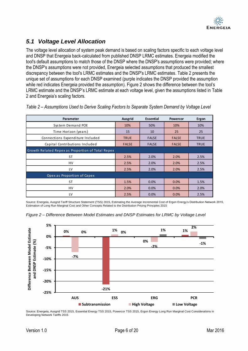
5.1 Voltage Level Allocation

The voltage level allocation of system peak demand is based on scaling factors specific to each voltage level and DNSP that Energeia back-calculated from published DNSP LRMC estimates. Energeia modified the tool's default assumptions to match those of the DNSP where the DNSP's assumptions were provided; where the DNSP's assumptions were not provided, Energeia selected assumptions that produced the smallest discrepancy between the tool's LRMC estimates and the DNSP's LRMC estimates. Table 2 presents the unique set of assumptions for each DNSP examined (purple indicates the DNSP provided the assumption while red indicates Energeia provided the assumption). Figure 2 shows the difference between the tool’s LRMC estimate and the DNSP’s LRMC estimate at each voltage level, given the assumptions listed in Table 2 and Energeia’s scaling factors.

Table 2 – Assumptions Used to Derive Scaling Factors to Separate System Demand by Voltage Level

Source: Energeia, Ausgrid Tariff Structure Statement (TSS) 2015, Estimating the Average Incremental Cost of Ergon Energy’s Distribution Network 2015,

Estimation of Long Run Marginal Cost and Other Concepts Related to the Distribution Pricing Principles 2015

Figure 2 – Difference Between Model Estimates and DNSP Estimates for LRMC by Voltage Level

Source: Energeia, Ausgrid TSS 2015, Essential Energy TSS 2015, Powercor TSS 2015, Ergon Energy Long Run Marginal Cost Considerations in

Developing Network Tariffs 2015

Parameter Ausgrid Essential Powercor Ergon

System Demand POE 10% 50% 10% 10%

Time Horizon (years ) 15 10 25 25

Connections Expenditure Included TRUE FALSE FALSE TRUE

Capita l Contributions Included FALSE FALSE FALSE TRUE

Growth Related Repex as Proportion of Total Repex

ST 2.5% 2.0% 2.0% 2.5%

HV 2.5% 2.0% 2.0% 2.5%

LV 2.5% 2.0% 2.0% 2.5%

Opex as Proportion of Capex

ST 1.5% 0.0% 0.0% 1.5%

HV 2.0% 0.0% 0.0% 2.0%

LV 2.5% 0.0% 0.0% 2.5%

0%

-21%

0%

1%

-7%

1%

-2%

2%0% 0%

1%

-1%

-25%

-20%

-15%

-10%

-5%

0%

5%

AUS ESS ERG PCR

Dif

fere

nce

Be

twe

en

Mo

de

l Est

imat

e

and

DN

SP E

stim

ate

(%

)

Subtransmission High Voltage Low Voltage


5.2 Network Type Allocation

To decompose annual incremental demand at each voltage level into CBD, urban, short rural (SR) and long rural (LR) annual incremental demand, the tool uses ratios derived from each network’s Augex Model (RIN Table 2.4.6). As shown in Figure 3, RIN Table 2.4.6 contains a breakdown of capex and capacity added over the 5 year forecast period by network type for only two asset groups: distribution substations and HV feeders. Figure 4 maps each network type allocation to each asset group in RIN Table 2.4.6 for which there is a capacity added breakdown by network type.

Figure 3 – Summary of Augex Model Outputs


Figure 4 – Network Type Allocation of Demand Mapped to Asset Group in RIN Table 2.4.6

5.3 Projection

The annual incremental demand forecasts are projected 20 years using the average growth rate over the 5-year forecast period to represent demand over the long term. However, the time horizon is configurable – the shorter the time horizon, the more weight is given to the DNSP's 5 year forecasts.

In the tool, the demand scaling factor can be adjusted to reflect the user's view on how representative the DNSP's 5 year forecast peak demand is of the long term average. If the user considers the DNSP's 5 year forecast demand to be above average, this percentage should be set to below 100%; it should be set to above 100% if the user considers the DNSP's 5 year forecast demand to be below average. Changing the demand scaling factor only affects the demand forecast after the first 5 years.

6 Incremental Capex Growth-related capex is composed of augmentation expenditure (augex), a proportion of replacement expenditure (repex), connections expenditure (connex) and capitalised network and corporate overheads.

6.1 Incremental Augex

AER defines annual incremental augex as the additional capital expenditure required to build or upgrade network assets to support changes in demand or to maintain quality, reliability and security of supply in accordance with legislated requirements2.

2 AER Better Regulation: Expenditure Forecast Assessment Guideline for Electricity Distribution, p18


6.1.1 Voltage Level Allocation

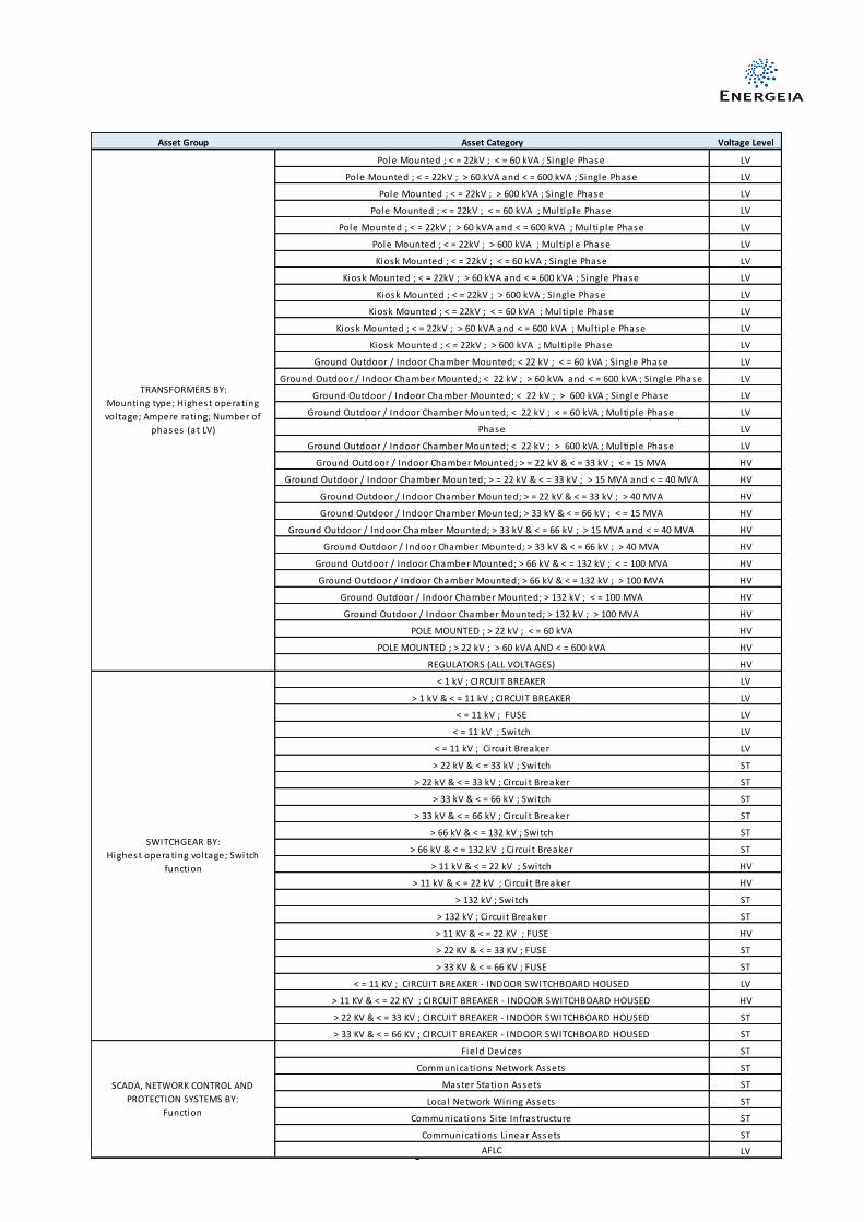
Augex is summarised in RIN Table 2.3.4. RIN Table 2.3.1 is used to separate augex on subtransmission substations and switching stations from augex on zone substations. This separation is necessary, given the tool’s assumption that subtransmission substations and switching stations are part of the subtransmission network while zone substations are part of the high voltage network. Table 3 shows how each entry in RIN Table 2.3.4 is allocated to a voltage level.

Table 3 – Stratification of Asset Categories by Voltage Level

6.1.2 Network Type Allocation

To decompose augex at each voltage level into CBD, urban, SR and LR augex, the tool uses ratios derived from each network’s Augex Model (RIN Table 2.4.6. Figure 5 maps each network type allocation of augex to each asset group in RIN Table 2.4.6 for which there is a capex breakdown by network type.

RIN Table 2.3.4 Asset Group Energeia Model Asset Group Voltage Level

Subtransmiss ion Lines Subtransmiss ion Lines

Subtransmiss ion Substations , Switching Stations

Zone Substations

HV Feeders HV Feeders

HV Feeders - Land Purchases and Easements HV Feeders - Land Purchases and Easements

Distribution Substations Distribution Substations

Distribution Substations - Land Purchases and

Easements

Distribution Substations - Land Purchases and

Easements

LV Feeders LV Feeders

LV Feeders - Land Purchases and Easements LV Feeders - Land Purchases and Easements

Other Assets Other Assets N/A

Subtransmiss ion

Subtransmiss ion Substations , Switching Stations ,

Zone Substations

High Voltage

Low Voltage


Figure 5 – Network Type Allocation of Augex Mapped to Asset Group in RIN Table 2.4.6

6.2 Incremental Repex

AER defines annual incremental repex as the capital expenditure associated with asset replacement driven by economic condition. This applies irrespective of any upgrade to the asset above the modern equivalent asset that may be done when assets are replaced at the end of their economic lives3.

There are two types of repex that need to be accounted for in the AIC calculation: first, repex on existing assets and secondly, repex on future augmentation assets.

Although repex on existing assets is not usually associated with demand growth, modern equivalent assets typically have higher capacity than those they replace. Energeia therefore assumes annual incremental repex is 2.5%4 of total repex, although this percentage is configurable.

Repex on future augmentation assets is incorporated into the AIC calculation by applying the Excel PMT function to augex. The PMT function calculates annualised capital expenditure, assuming constant payments, constant interest rates (equal to the DNSP-specific real WACC) and a configurable average asset lifetime.


4 Including capitalized network and corporate overheads

126254

Highlight



Repex is specified on an asset category level in RIN Table 2.2.1. In the tool, each asset category is categorised based on the corresponding voltage level (see Table 7 in Appendix 3 for mapping). Where an asset category spans across multiple voltage levels (such as ‘staking of wooden poles’), repex is generally allocated based on the overhead line circuit length at each voltage level, sourced from RIN Table 3.5.1.1.


To decompose repex at each voltage level into CBD, urban, SR and LR repex, the tool uses ratios derived from each network’s Augex Model (RIN Table 2.4.6). Figure 6 maps each network type allocation of repex to each asset group in RIN Table 2.4.6 for which there is a capex breakdown by network type.

Figure 6 – Network Type Allocation of Repex Mapped to Asset Group in RIN Table 2.4.6

6.3 Incremental Connex

AER defines annual incremental connex as the capital expenditure required to augment the network to support the additional demand associated with new customer connections and other customer-related works5.


Connex is displayed in RIN Table 2.5.2 based on customer type (residential, commercial/industrial, subdivision and embedded generation) and voltage level (ST, HV and LV). For the purpose of calculating AIC values, connex is aggregated by voltage level.




To decompose connex at each voltage level into CBD, urban, SR and LR connex, the tool uses the ratio of forecast new connections segmented by network type derived from data in RIN Table 3.4.2.2 for each DNSP.

Capital contributions by customers, sourced from RIN Table 2.1.1, are deducted from connections expenditure in the same ratio as the connections expenditure.

The inclusion of connex and customer contributions is configurable in the tool.

6.4 Incremental Overheads

Capitalised network and corporate overheads, sourced from RIN Table 2.1.1, are apportioned to augex, repex and connex based on each investment driver’s relative contributions to total capex.

6.5 Projection

Annual incremental augex, repex and connex are then projected 20 years beyond the 5-year forecast period using the average growth rate during the 5-year forecast period to represent incremental capital expenditure over the long term. However, the time horizon is configurable.

The augex scaling factor can be adjusted to reflect the user's view on how representative the DNSP's 5 year forecast augex is of the long term average. Only affects the augex forecast after the first 5 years. If the user considers the DNSP's 5 year forecast augex to be above average, this percentage should be set to below 100%; this percentage should be set to above 100% if the user considers the DNSP's 5 year forecast augex to be below average. The augex scaling factor only affects the augex forecast after the first 5 years.

7 Incremental Opex AER defines opex as the non-capital cost of running an electricity network and maintaining the assets6. More specifically, annual incremental opex is the additional operating and maintenance costs (including vegetation management, maintenance, emergency response, non-network costs, and network and corporate overheads) that are associated with the assets that must be built or upgraded to support changes in demand, and the existing assets that are likely to fail more often due to higher utilisation rates.

7.1 Voltage Level Allocation

Assets at higher voltage levels tend to be more capital intensive whereas those at lower voltage levels tend to be more maintenance intensive. This is reflected in Energeia’s assumptions relating to opex as a proportion of growth-related capex (including overheads) at each voltage level. The set of proportions listed in Table 4 are used across all four DNSPs, although they are configurable.



Table 4 – Opex as a Proportion of Capex by Voltage Level

As opex on newly commissioned assets is usually phased in during the few years immediately following the asset’s commissioning, the percentages listed in Table 5 are also applied to growth-related capex to produce the annual incremental opex at each voltage level.

Table 5 – Opex Scaling Factors for Each Year Following the Asset’s Commissioning

7.2 Network Type Allocation

Annual incremental opex at each voltage level was converted to annual incremental opex at each network type based on each network type’s contribution to total capex at each voltage level.

7.3 Projection

Annual incremental opex is then projected 20 years beyond the 5-year forecast period using the average growth rate during the 5-year forecast period to represent incremental opex over the long term. However, the time horizon is configurable.

8 Assumptions and Limitations The tool assumes that the RIN data is correct and derived using a consistent approach across the DNSPs.

The tool assumes that the 5-year forecast period in the RINs is indicative of the next 5-25 years (depending on the tool’s configuration) for network demand and growth-related expenditure.

The tool assumes a constant allocation of demand, capex and opex across the different network types over time.

The accuracy of the tool is limited by the extent to which network demand and growth-related expenditure are broken down by voltage level and network type in the RINs. Table 6Error! Reference source not found. shows which model inputs were provided by voltage level and which were provided by network type in the RINs.

Table 6 – Granularity of RIN Data for each Model Input

Voltage Level Opex as Proportion of Capex

ST 1.50%

HV 2.00%

LV 2.50%

Year 0 1 2 3 4

Percentage 0% 60% 0% 0% 40%

Incremental Annual Opex as a Percentage of Capex

InputSystem Level Data

Provided in the RINs

Voltage Level Breakdown


Network Type Breakdown


Incremental Augmentation Expenditure

Incremental Replacement Expenditure

Incremental Connections Expenditure

Incremental Operations and Maintenance Expenditure

Incremental Demand


Appendix 1 – Approaches to Calculating LRMC Three approaches for the calculation of LRMC were considered.

Average Incremental Cost (AIC)

Turvey Incremental Cost (TIC)

Long Run Incremental Cost (LRIC)

The average incremental cost was deemed most appropriate given the aims of the project. This section outlines the three approaches and the justification for the selection of the AIC.

A1.1 Average Incremental Cost Approach

Calculating the AIC involves the following three steps:

1. Forecast peak demand over a future time horizon (e.g. 25 years)

2. Develop a least cost program of network capacity augmentation to ensure that future network capacity can support future peak demand, to the extent dictated by the relevant reliability standards

3. Calculate AIC by dividing the present value of the expected costs of the augmentation program by the present value of the additional demand supplied. The expected costs of the augmentation program refers to both capital costs and marginal operating costs, while the additional demand supplied refers to the demand over and above that which is currently being supplied rather than that which could be supplied.

There are two key advantages to the AIC over other LRMC approaches: the outputs are not as sensitive to initial conditions and it is not as effort and data intensive.

The main disadvantage of the AIC is that it does not attempt to connect a particular increment of demand with the resulting change in cost. Instead, the AIC approach uses average future capital costs to estimate the likely marginal costs associated with a change in demand. This does not align with the inherently lumpy nature of network investment where an extra 1 MW of demand at a constrained zone substation may require millions of dollars of additional investment while an extra 1 MW of demand at a newly established zone substation would require very little additional expenditure.

A1.2 Turvey Incremental Cost Approach

Calculating the TIC involves the following four steps:

1. Forecast peak demand over a future time horizon (e.g. 25 years)

2. Develop a least cost program of network capacity augmentation to ensure that future network capacity can support future peak demand, to the extent dictated by the relevant reliability standards

3. Increase or decrease forecast peak demand by a small, but permanent amount and recalculate the least cost program of network capacity augmentation required to satisfy the revised level of peak demand

4. Calculate TIC by dividing the present value of the change in expected costs of the augmentation program by the present value of the change in additional demand supplied. The expected costs of the augmentation program refers to both capital costs and marginal operating costs, while the additional demand supplied refers to the demand over and above that which is currently being supplied rather than that which could be supplied.


The main advantage of the TIC is that it focuses on the specific cost implications of an increment of demand. It therefore more accurately reflects the nature of network investment and the concept of a long run marginal cost.

The primary disadvantage of the TIC is that the outputs are highly sensitive to initial conditions, the timing of planned investment, the lumpiness of investment and the incremental size of demand. In this way, calculating LRMC using the Turvey approach is typically a more subjective and arbitrary exercise than calculating LRMC using the other approaches.

Another shortcoming of the TIC is that it is resource and data intensive, requiring two estimates of capital and operating expenditure programs, given two sets of demand forecasts.

A1.3 Long Run Incremental Cost Approach

Calculating the LRIC involves calculating the annualised cost of augmentation necessary to support a specified increment in demand. The most common example of this approach is the Common Distribution Charging Methodology (CDCM), which forms the basis for distribution tariffs in the United Kingdom. This model is based upon the creation of a hypothetical network for the supply of 500 MW of demand, using the spatial characteristics and standardised equipment typical for the distributor.

The key benefit of the LRIC is that it can be used to accurately estimate a LRMC specific to a particular network type (e.g. CBD, urban, short rural or long rural).

The main shortfalls of the LRIC are that it is complex and costly to carry out, and the outputs are sensitive to starting conditions.

A1.4 Energeia’s Approach to Calculating LRMC

Energeia views the AIC approach as the most feasible and appropriate approach to use because it satisfies the ISF’s requirements, is commonly employed by Distribution Network Service Providers (DNSPs), is less sensitive to the modeller’s assumptions than the other approaches and is less complex than the other approaches. The publically available regulatory information notice (RIN) data includes all key information needed to perform an LRMC calculation using the AIC method at the system level, some information at the voltage level and little information at the spatial level (see Section 8). This meets ISF’s requirements of transparency (publically available data), consistency (data provided using the same calculation methodology) and auditability (AER audits the RIN data).


Appendix 2 – Approach to Segmenting AIC by Network Type Two approaches for the segmentation of system AIC by network type were considered.

Augex Model

Augex Projects

The Augex Model was deemed most appropriate given the aims of the project. This section outlines the two approaches and the justification for the selection of the Augex Model.

A2.1 Augex Model Approach

The Augex Model is a predictive model employed by the AER that relies on capacity factors to identify parts of the network that may require augmentation, and unit costs to derive an augex forecast for each DNSP over the 5-year forecast period. Given the different network configurations, operating conditions and non-standard techniques for data collection and presentation by different DNSPs, the outputs of the Augex Model are not necessarily accurate or comparable, especially during periods of changing levels of demand growth and/or changing network reliability standards.

The Augex Model approach to segmenting system AIC by network type involves the following eight steps:

1. As part of each network’s Augex Model, forecast capex on HV feeders and distribution substations is split into CBD, urban, SR and LR (in RIN Table 2.4.6). Using these values, calculate two capex ratios for each DNSP: one for HV feeders and one for distribution substations.

2. Forecast capacity added in MVA on HV feeders and distribution substations is similarly separated in the Augex Model. Use these values to calculate two incremental demand ratios for each DNSP: one for HV feeders and one for distribution substations.

3. Apply the capex ratio for HV feeders obtained in Step 1 to augex on ST lines, ST substations, switching stations, HV feeders and HV feeders – land. Apply the capex ratio for distribution substations obtained in Step 1 to augex on distribution substations, distribution substations – land, LV feeders and LV feeders - land. Assume the augex zone substations is split evenly among CBD, urban, SR and LR.

4. Apply the capex ratio for HV feeders obtained in Step 1 to HV repex, and the capex ratio for distribution substations to LV repex. Assume ST repex is split evenly among CBD, urban, SR and LR.

5. Leave opex as a certain proportion of capex.

6. Allocate future connex across the four network types (CBD, urban, SR and LR) based on their relative contributions to the number of forecast connections over the next 5 years.

7. Apply the incremental demand ratio for HV feeders obtained in Step 2 to HV incremental demand, and the incremental demand ratio for distribution substations obtained in Step 2 to LV incremental demand. Assume ST incremental demand is split evenly among CBD, urban, SR and LR.

8. Calculate each DNSP’s AIC for CBD, urban, SR and LR network types by dividing the total incremental capex and opex for each network type over the incremental demand for each network type.

The primary advantage of the Augex Model approach is that it provides detail on the average cost in $/MVA added of distribution substations and HV feeders at the network type level, which is likely to be greater than the variation in the average cost in $/MVA added of zone substations at the network type level.

The main disadvantage of the Augex Model approach is that the outputs of the Augex Model are calculated at a very high level and therefore should not be regarded as highly accurate.


Another disadvantage is that the Augex Model does not provide a breakdown of the average cost in $/MVA of subtransmission assets by network type.

A2.2 Augex Projects Approach

The Augex Projects approach to segmenting system AIC by network type involves the following three steps:

1. Using each network’s list of proposed augex projects for the current regulatory period (in RIN Table 2.3.1), calculate the average $/MVA for CBD, urban, SR and LR zone substations.

2. Calculate a ratio specific to each network based on the values found in Step 1.

3. Apply the ratios found in Step 2 to each DNSP’s system AIC.

The main advantage of the Augex Projects approach is that it relies on real project costs.

The main disadvantage is that data is quite limited in this area, with the number of new or upgraded zone substations ranging from 3–20 per DNSP. Moreover, based on the data that is available, there seems to be little variation in the average $/MVA for CBD, urban, SR and LR zone substations.

A2.2 Energeia’s Approach to Segmenting System AIC by Network Type

As the Augex Model provides detail on the average costs ($/MVA) at the HV and LV levels, where average costs are more likely to differ among different network types than at the ST level, Energeia chose to adopt this methodology over the Augex Projects methodology. To reduce the effect of inaccuracy or inconsistency across Augex Model outputs across DNSPs, only the ratios of capex and demand among network types were used – rather than the nominal values.


Appendix 3 – Repex Voltage Allocation Table 7 shows how each repex asset category in RIN Table 2.2.1 is mapped to a voltage level.

Table 7 – Mapping of Repex Asset Categories in RIN Table 2.2.1 to Voltage Levels

Asset Group Asset Category Voltage Level

Staking of a wooden pole LV+HV

˂ = 1 kV; Wood LV

> 1 kV & < = 11 kV; Wood LV

˃ 11 kV & < = 22 kV; Wood HV

> 22 kV & < = 66 kV; Wood ST

> 66 kV & < = 132 kV; Wood ST

> 132 kV; Wood ST

˂ = 1 kV; Concrete LV

> 1 kV & < = 11 kV; Concrete LV

˃ 11 kV & < = 22 kV; Concrete HV

> 22 kV & < = 66 kV; Concrete ST

> 66 kV & < = 132 kV; Concrete ST

> 132 kV; Concrete ST

˂ = 1 kV; Steel LV

> 1 kV & < = 11 kV; Steel LV

˃ 11 kV & < = 22 kV; Steel HV

> 22 kV & < = 66 kV; Steel ST

> 66 kV & < = 132 kV; Steel ST

> 132 kV; Steel ST

OTHER - Bol lards and unknown Other

Other Other

˂ = 1 kV LV

> 1 kV & < = 11 kV LV

˃ 11 kV & < = 22 kV HV

> 22 kV & < = 66 kV ST

> 66 kV & < = 132 kV ST

> 132 kV ST

˃ 11 kV & < = 22 kV ; SWER HV

˃ 11 kV & < = 22 kV ; Single-Phase HV

˃ 11 kV & < = 22 kV ; Multiple-Phase HV

> 11 kV & < = 22 kV HV

> 22 kV & < = 33 kV ST

> 33 kV & < = 66 kV ST

> 132 kV ST

˂ = 11 kV ; Res identia l ; Simple Type LV

˂ = 11 kV ; Commercia l & Industria l ; Simple Type LV

< = 11kV; RESIDENTIAL ; SIMPLE ; OVERHEAD LV

< = 11kV; RESIDENTIAL ; SIMPLE ; UNDERGROUND LV

< = 11kV; COMMERCIAL & INDUSTRIAL ; SIMPLE ; OVERHEAD LV

< = 11kV; COMMERCIAL & INDUSTRIAL ; SIMPLE ; UNDERGROUND LV

˂ = 11 kV ; Res identia l ; Complex Type LV

˂ = 11 kV ; Commercia l & Industria l ; Complex Type LV

˂ = 11 kV ; Subdivis ion ; Complex Type LV

> 11 kV & < = 22 kV ; Commercia l & Industria l HV

> 11 kV & < = 22 kV ; Subdivis ion HV

> 22 kV & < = 33 kV ; Commercia l & Industria l ST

> 22 kV & < = 33 kV ; Subdivis ion ST





> 132 kV ; Commercia l & Industria l ST

> 132 kV ; Subdivis ion ST

POLES BY:

Highest operating voltage; Materia l

type; Staking (i f wood)

POLE TOP STRUCTURES BY:

Highest operating voltage

OVERHEAD CONDUCTORS BY:

Highest operating voltage; Number of

phases (at HV)

UNDERGROUND CABLES BY:

Highest operating voltage

SERVICE LINES BY:

Connection voltage; Customer type;

Connection complexi ty



Pole Mounted ; < = 22kV ; < = 60 kVA ; Single Phase LV

Pole Mounted ; < = 22kV ; > 60 kVA and < = 600 kVA ; Single Phase LV

Pole Mounted ; < = 22kV ; > 600 kVA ; Single Phase LV

Pole Mounted ; < = 22kV ; < = 60 kVA ; Multiple Phase LV

Pole Mounted ; < = 22kV ; > 60 kVA and < = 600 kVA ; Multiple Phase LV

Pole Mounted ; < = 22kV ; > 600 kVA ; Multiple Phase LV

Kiosk Mounted ; < = 22kV ; < = 60 kVA ; Single Phase LV

Kiosk Mounted ; < = 22kV ; > 60 kVA and < = 600 kVA ; Single Phase LV

Kiosk Mounted ; < = 22kV ; > 600 kVA ; Single Phase LV

Kiosk Mounted ; < = 22kV ; < = 60 kVA ; Multiple Phase LV

Kiosk Mounted ; < = 22kV ; > 60 kVA and < = 600 kVA ; Multiple Phase LV

Kiosk Mounted ; < = 22kV ; > 600 kVA ; Multiple Phase LV

Ground Outdoor / Indoor Chamber Mounted; ˂ 22 kV ; < = 60 kVA ; Single Phase LV

Ground Outdoor / Indoor Chamber Mounted; ˂ 22 kV ; > 60 kVA and < = 600 kVA ; Single Phase LV

Ground Outdoor / Indoor Chamber Mounted; ˂ 22 kV ; > 600 kVA ; Single Phase LV

Ground Outdoor / Indoor Chamber Mounted; ˂ 22 kV ; < = 60 kVA ; Multiple Phase LVGround Outdoor / Indoor Chamber Mounted; ˂ 22 kV ; > 60 kVA and < = 600 kVA ; Multiple

Phase LV

Ground Outdoor / Indoor Chamber Mounted; ˂ 22 kV ; > 600 kVA ; Multiple Phase LV

Ground Outdoor / Indoor Chamber Mounted; > = 22 kV & < = 33 kV ; < = 15 MVA HV

Ground Outdoor / Indoor Chamber Mounted; > = 22 kV & < = 33 kV ; > 15 MVA and < = 40 MVA HV

Ground Outdoor / Indoor Chamber Mounted; > = 22 kV & < = 33 kV ; > 40 MVA HV

Ground Outdoor / Indoor Chamber Mounted; > 33 kV & < = 66 kV ; < = 15 MVA HV

Ground Outdoor / Indoor Chamber Mounted; > 33 kV & < = 66 kV ; > 15 MVA and < = 40 MVA HV

Ground Outdoor / Indoor Chamber Mounted; > 33 kV & < = 66 kV ; > 40 MVA HV

Ground Outdoor / Indoor Chamber Mounted; > 66 kV & < = 132 kV ; < = 100 MVA HV

Ground Outdoor / Indoor Chamber Mounted; > 66 kV & < = 132 kV ; > 100 MVA HV

Ground Outdoor / Indoor Chamber Mounted; > 132 kV ; < = 100 MVA HV

Ground Outdoor / Indoor Chamber Mounted; > 132 kV ; > 100 MVA HV

POLE MOUNTED ; > 22 kV ; < = 60 kVA HV

POLE MOUNTED ; > 22 kV ; > 60 kVA AND < = 600 kVA HV

REGULATORS (ALL VOLTAGES) HV

< 1 kV ; CIRCUIT BREAKER LV

> 1 kV & < ≈ 11 kV ; CIRCUIT BREAKER LV

˂ = 11 kV ; FUSE LV

˂ = 11 kV ; Switch LV

˂ = 11 kV ; Ci rcui t Breaker LV

> 22 kV & < = 33 kV ; Switch ST

> 22 kV & < = 33 kV ; Ci rcui t Breaker ST

> 33 kV & < = 66 kV ; Switch ST


> 66 kV & < = 132 kV ; Switch ST


> 11 kV & < = 22 kV ; Switch HV

> 11 kV & < = 22 kV ; Ci rcui t Breaker HV

> 132 kV ; Switch ST

> 132 kV ; Ci rcui t Breaker ST

> 11 KV & < = 22 KV ; FUSE HV

> 22 KV & < = 33 KV ; FUSE ST

> 33 KV & < = 66 KV ; FUSE ST

˂ = 11 KV ; CIRCUIT BREAKER - INDOOR SWITCHBOARD HOUSED LV

> 11 KV & < = 22 KV ; CIRCUIT BREAKER - INDOOR SWITCHBOARD HOUSED HV

> 22 KV & < = 33 KV ; CIRCUIT BREAKER - INDOOR SWITCHBOARD HOUSED ST

> 33 KV & < = 66 KV ; CIRCUIT BREAKER - INDOOR SWITCHBOARD HOUSED ST

Field Devices ST

Communications Network Assets ST

Master Station Assets ST

Local Network Wiring Assets ST

Communications Si te Infrastructure ST

Communications Linear Assets ST

AFLC LV

SWITCHGEAR BY:

Highest operating voltage; Switch

function

SCADA, NETWORK CONTROL AND

PROTECTION SYSTEMS BY:

Function

TRANSFORMERS BY:

Mounting type; Highest operating

voltage; Ampere rating; Number of

phases (at LV)



Luminaires ; Major Road Other

Luminaires ; Minor Road Other

Brackets ; Major Road Other

Brackets ; Minor Road Other

Lamps ; Major Road Other

Lamps ; Minor Road Other

Poles / Columns ; Major Road Other

Poles / Columns ; Minor Road Other

DISTRIBUTION SUBSTATIONS - OTHER LV

DISTRIBUTION VOLTAGE REGULATION LV

TOWERS - > = 33 kV ; ANTI-CLIMB DEVICES ST

TOWERS - > = 33 kV TOWER FOOTINGS ST

TOWERS - > = 33 kV TOWER REFURBISHMENT ST

ZONE & SUBTRANSMISION SUBSTATIONS - OTHER HV+ST

BUILDINGS Other

Zone CLC equipment (Electronic) HV

Zone Genera l (including spares) HV

Zone prot. & control equipment (Electronic) HV

STS Protection & Control (Electronic) ST

STS Reactors and Capaci tors ST

Sub-Transmiss ion Main OH Easement ST

STS Bui lding (incl sw. s tns ) ST

STS Communications ST

STS DC Systems ST

STS Genera l (including spares) ST

Zone Reactors and Capaci tors HV

Environmental Management LV+HV+ST

PLANT AND STATIONS MISCELLANEOUS HV

Zone Substation Major Bui lding / Property / Faci l i ties HV

VBRC SWER ACRs HV

TV Interference Replacement Capita l Other

CURRENT TRANSFORMERS HV

VOLTAGE TRANSFORMERS HV

CAPACITOR BANKS HV

SVC HV

Orange North - TransGrid rebui ld Orange 66kV busbar - REFURBISHMENT ST

Recti fication of low clearance infringements on subtransmiss ion feeders - REFURBISHMENT ST

Tamworth - TransGrid 132/66kV substation - relocate 66kV feeders - REFURBISHMENT ST

Terranora to QLD border - refurbish 110kV towers in l ine with Powerl ink - REFURBISHMENT ST

Yarrandale to Gi lgandra - rebui ld exis ting 66kV feeder - REFURBISHMENT ST

Wagga Copeland St - TransGrid 132/66kV sub - relocate 66kV feeders - REFURBISHMENT ST

Queanbeyan TG to Googong Town ZS Refurbish Line 975 - REFURBISHMENT ST

Pole top refurbishment of Taree to Forster 66kV feeders - REFURBISHMENT STPole top refurbishment of Dubbo to Nyngan 132kV feeder 943/1, 943/2 and 9GU -

REFURBISHMENT ST

Gunnedah to Narrabri Tee via Boggabri - refurbish 66kV feeders - REFURBISHMENT ST

Taree - TransGrid 132/66/33kV substation - relocate 33kV feeders - REFURBISHMENT HV

Customer Metering and Load Control LV

S&W Accrual and Other Adjustments Other

Dis t Lines & Cables , Sub Trans Lines ,LV Lines (ba l . i tems) - REFURBISHMENT Other

Subtransmiss ion Lines (ba lancing Items) - - REFURBISHMENT ST

PUBLIC LIGHTING BY:

Asset type ; Lighting obl igation

OTHER BY:

DNSP defined

lrmc methodology paper prepared by energeia … · lrmc methodology paper prepared by energeia for...

Documents