Machine Learning

Lecture 9

Support Vector Machines

G53MLE | Machine Learning | Dr Guoping Qiu 1

Based on slides from Prof. Ray Mooney

2

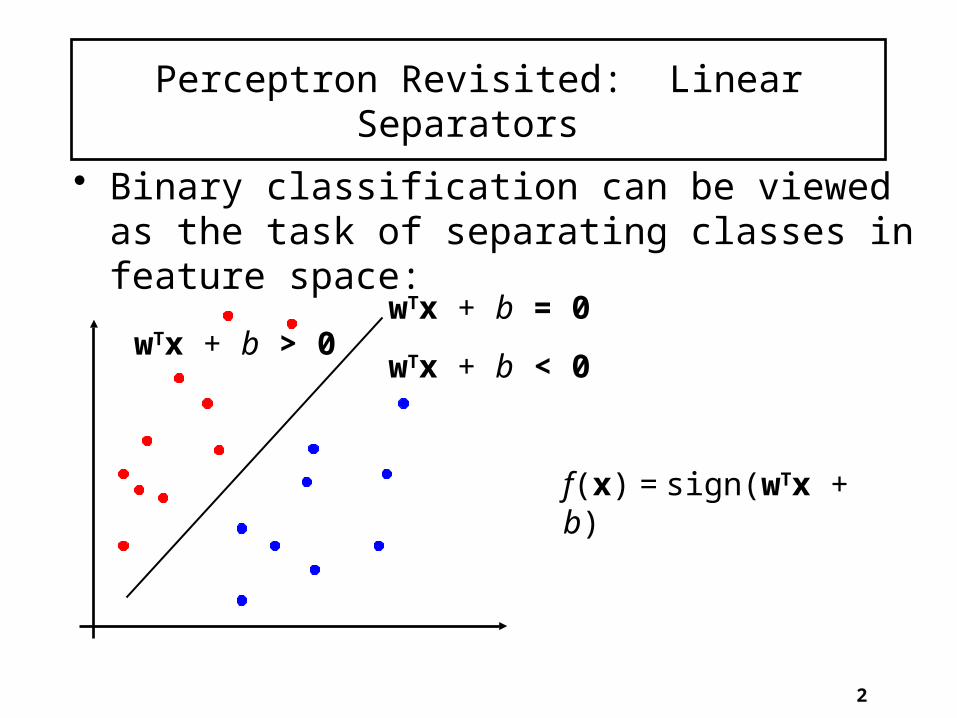
Perceptron Revisited: Linear Separators

• Binary classification can be viewed as the task of separating classes in feature space:

wTx + b = 0

wTx + b < 0wTx + b > 0

f(x) = sign(wTx + b)

3

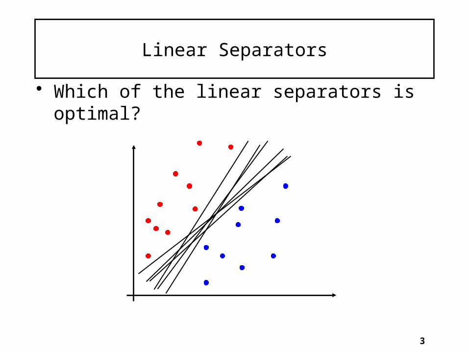
Linear Separators

• Which of the linear separators is optimal?

4

Classification Margin

• Distance from example xi to the separator is

• Examples closest to the hyperplane are support vectors. • Margin ρ of the separator is the distance between support vectors.

w

xw br i

T

r

ρ

5

Maximum Margin Classification

• Maximizing the margin is good according to intuition and PAC theory.

• Implies that only support vectors matter; other training examples are ignorable.

6

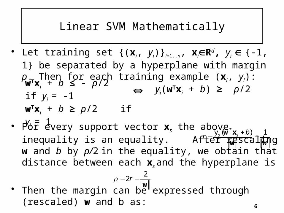
Linear SVM Mathematically

• Let training set {(xi, yi)}i=1..n, xiRd, yi {-1, 1} be separated by a hyperplane with margin ρ. Then for each training example (xi, yi):

• For every support vector xs the above inequality is an equality. After rescaling w and b by ρ/2 in the equality, we obtain that distance between each xs and the hyperplane is

• Then the margin can be expressed through (rescaled) w and b as:

wTxi + b ≤ - ρ/2 if yi = -1wTxi + b ≥ ρ/2 if yi = 1

w

22 r

ww

xw 1)(y

br s

Ts

yi(wTxi + b) ≥ ρ/2

7

Linear SVMs Mathematically (cont.)

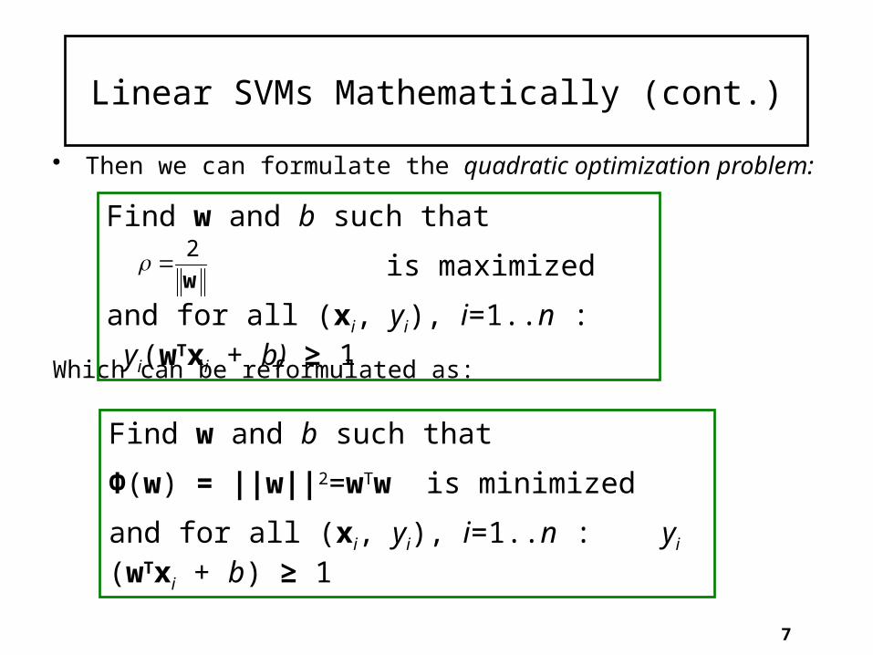
• Then we can formulate the quadratic optimization problem:

Which can be reformulated as:

Find w and b such that

is maximized

and for all (xi, yi), i=1..n : yi(wTxi + b) ≥ 1w

2

Find w and b such that

Φ(w) = ||w||2=wTw is minimized

and for all (xi, yi), i=1..n : yi (wTxi + b) ≥ 1

8

Solving the Optimization Problem

• Need to optimize a quadratic function subject to linear constraints.• Quadratic optimization problems are a well-known class of mathematical

programming problems for which several (non-trivial) algorithms exist.• The solution involves constructing a dual problem where a Lagrange

multiplier αi is associated with every inequality constraint in the primal (original) problem:

Find w and b such thatΦ(w) =wTw is minimized and for all (xi, yi), i=1..n : yi (wTxi + b) ≥ 1

Find α1…αn such that

Q(α) =Σαi - ½ΣΣαiαjyiyjxiTxj is maximized and

(1) Σαiyi = 0(2) αi ≥ 0 for all αi

9

The Optimization Problem Solution

• Given a solution α1…αn to the dual problem, solution to the primal is:

• Each non-zero αi indicates that corresponding xi is a support vector.

• Then the classifying function is (note that we don’t need w explicitly):

• Notice that it relies on an inner product between the test point x and the support vectors xi – we will return to this later.

• Also keep in mind that solving the optimization problem involved computing the inner products xi

Txj between all training points.

w =Σαiyixi b = yk - Σαiyixi Txk for any αk > 0

f(x) = ΣαiyixiTx + b

10

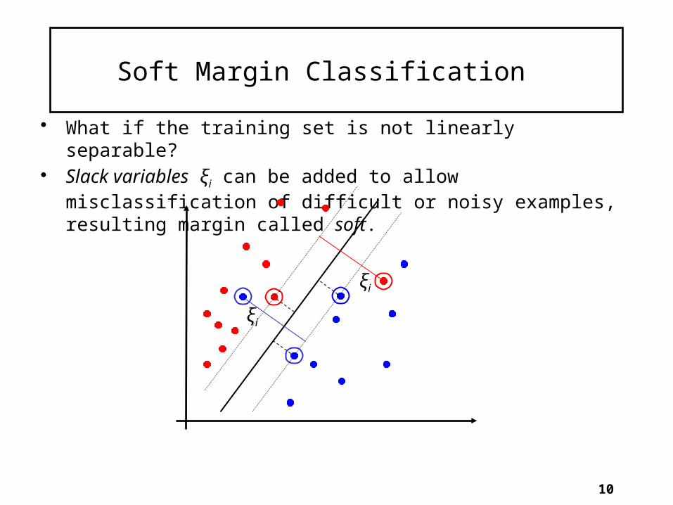
Soft Margin Classification

• What if the training set is not linearly separable?• Slack variables ξi can be added to allow misclassification of difficult or

noisy examples, resulting margin called soft.

ξi

ξi

11

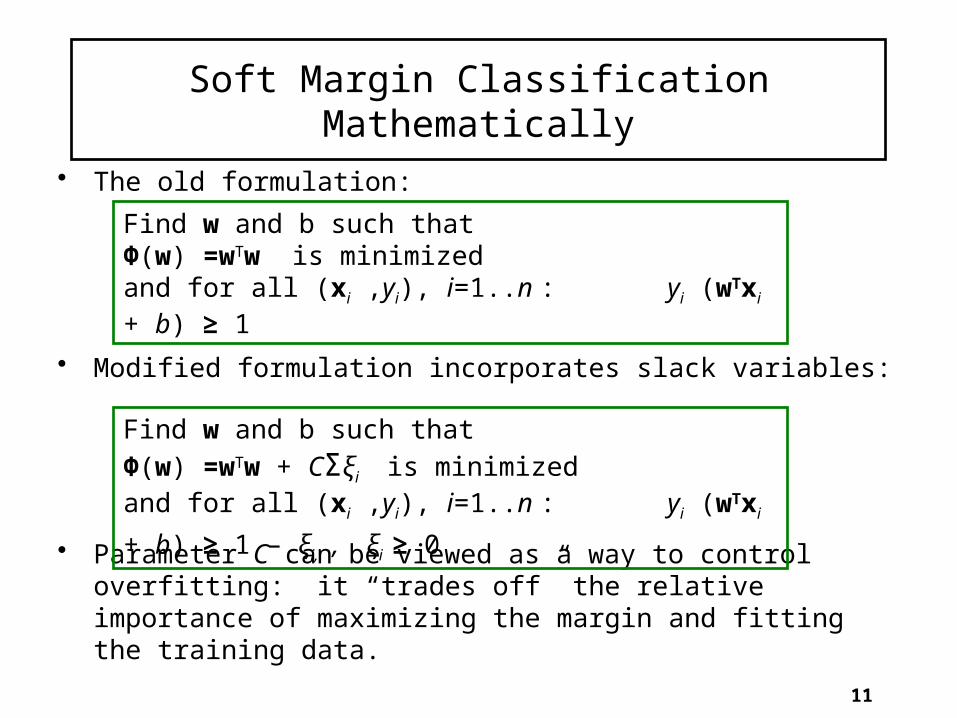
Soft Margin Classification Mathematically

• The old formulation:

• Modified formulation incorporates slack variables:

• Parameter C can be viewed as a way to control overfitting: it “trades off” the relative importance of maximizing the margin and fitting the training data.

Find w and b such thatΦ(w) =wTw is minimized and for all (xi ,yi), i=1..n : yi (wTxi + b) ≥ 1

Find w and b such that

Φ(w) =wTw + CΣξi is minimized

and for all (xi ,yi), i=1..n : yi (wTxi + b) ≥ 1 – ξi, , ξi ≥ 0

12

Soft Margin Classification – Solution

• Dual problem is identical to separable case (would not be identical if the 2-norm penalty for slack variables CΣξi

2 was used in primal objective, we would need additional Lagrange multipliers for slack variables):

• Again, xi with non-zero αi will be support vectors.

• Solution to the dual problem is:

Find α1…αN such that

Q(α) =Σαi - ½ΣΣαiαjyiyjxiTxj is maximized and

(1) Σαiyi = 0(2) 0 ≤ αi ≤ C for all αi

w =Σαiyixi

b= yk(1- ξk) - ΣαiyixiTxk for any k s.t. αk>0

f(x) = ΣαiyixiTx + b

Again, we don’t need to compute w explicitly for classification:

13

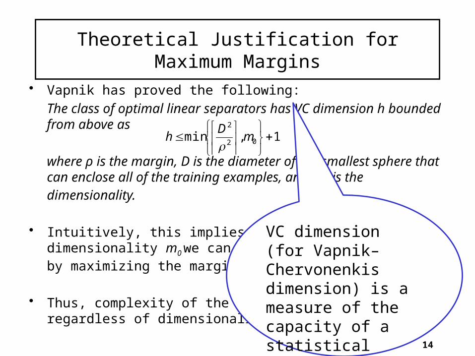
Theoretical Justification for Maximum Margins

• Vapnik has proved the following:

The class of optimal linear separators has VC dimension h bounded from above as

where ρ is the margin, D is the diameter of the smallest sphere that can enclose all of the training examples, and m0 is the dimensionality.

• Intuitively, this implies that regardless of dimensionality m0 we can minimize the VC dimension by maximizing the margin ρ.

• Thus, complexity of the classifier is kept small regardless of dimensionality.

1,min 02

2

m

Dh

14

Theoretical Justification for Maximum Margins

• Vapnik has proved the following:

The class of optimal linear separators has VC dimension h bounded from above as

where ρ is the margin, D is the diameter of the smallest sphere that can enclose all of the training examples, and m0 is the dimensionality.

• Intuitively, this implies that regardless of dimensionality m0 we can minimize the VC dimension by maximizing the margin ρ.

• Thus, complexity of the classifier is kept small regardless of dimensionality.

1,min 02

2

m

Dh

VC dimension (for Vapnik–Chervonenkis dimension) is a measure of the capacity of a statistical classification algorithm

15

Linear SVMs: Overview

• The classifier is a separating hyperplane.

• Most “important” training points are support vectors; they define the hyperplane.

• Quadratic optimization algorithms can identify which training points xi are support vectors with non-zero Lagrangian multipliers αi.

• Both in the dual formulation of the problem and in the solution training points appear only inside inner products:

Find α1…αN such that

Q(α) =Σαi - ½ΣΣαiαjyiyjxiTxj is maximized and

(1) Σαiyi = 0(2) 0 ≤ αi ≤ C for all αi

f(x) = ΣαiyixiTx + b

16

Non-linear SVMs

• Datasets that are linearly separable with some noise work out great:

• But what are we going to do if the dataset is just too hard?

• How about… mapping data to a higher-dimensional space:

0

0

0

x2

x

x

x

17

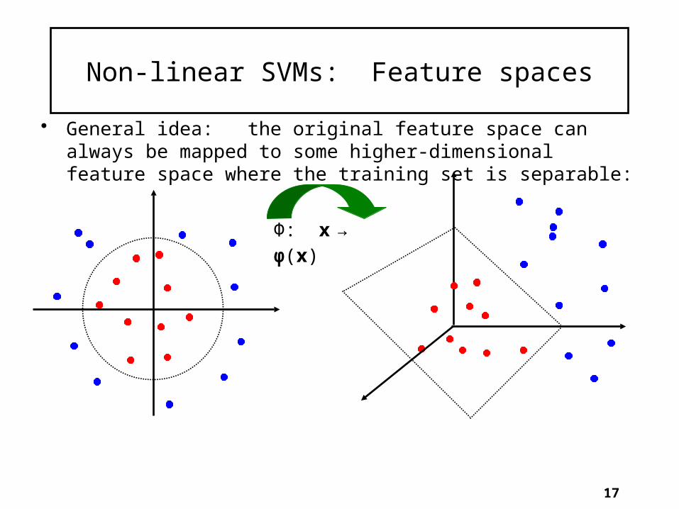
Non-linear SVMs: Feature spaces

• General idea: the original feature space can always be mapped to some higher-dimensional feature space where the training set is separable:

Φ: x → φ(x)

18

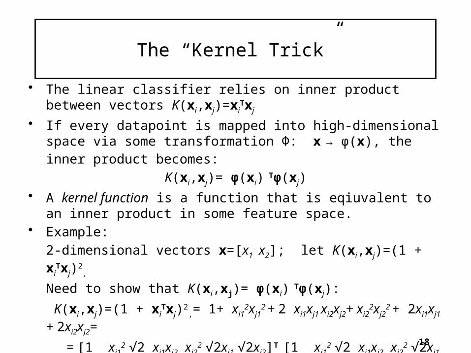
The “Kernel Trick”

• The linear classifier relies on inner product between vectors K(xi,xj)=xiTxj

• If every datapoint is mapped into high-dimensional space via some transformation Φ: x → φ(x), the inner product becomes:

K(xi,xj)= φ(xi) Tφ(xj)

• A kernel function is a function that is eqiuvalent to an inner product in some feature space.

• Example:

2-dimensional vectors x=[x1 x2]; let K(xi,xj)=(1 + xiTxj)2

,

Need to show that K(xi,xj)= φ(xi) Tφ(xj):

K(xi,xj)=(1 + xiTxj)2

,= 1+ xi12xj1

2 + 2 xi1xj1 xi2xj2+ xi2

2xj22 + 2xi1xj1 + 2xi2xj2=

= [1 xi12 √2 xi1xi2 xi2

2 √2xi1 √2xi2]T [1 xj12 √2 xj1xj2 xj2

2 √2xj1 √2xj2] =

= φ(xi) Tφ(xj), where φ(x) = [1 x1

2 √2 x1x2 x22 √2x1 √2x2]

• Thus, a kernel function implicitly maps data to a high-dimensional space (without the need to compute each φ(x) explicitly).

19

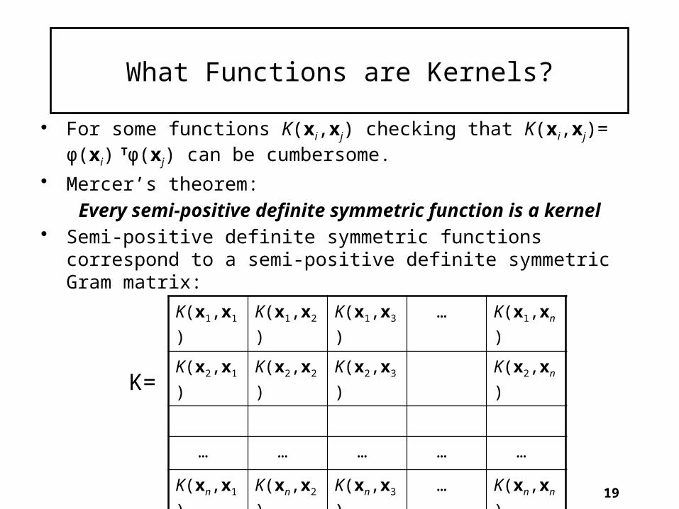
What Functions are Kernels?

• For some functions K(xi,xj) checking that K(xi,xj)= φ(xi) Tφ(xj) can be

cumbersome. • Mercer’s theorem:

Every semi-positive definite symmetric function is a kernel• Semi-positive definite symmetric functions correspond to a semi-positive

definite symmetric Gram matrix:

K(x1,x1) K(x1,x2) K(x1,x3) … K(x1,xn)

K(x2,x1) K(x2,x2) K(x2,x3) K(x2,xn)

… … … … …

K(xn,x1) K(xn,x2) K(xn,x3) … K(xn,xn)

K=

20

Examples of Kernel Functions

• Linear: K(xi,xj)= xiTxj

– Mapping Φ: x → φ(x), where φ(x) is x itself

• Polynomial of power p: K(xi,xj)= (1+ xiTxj)p

– Mapping Φ: x → φ(x), where φ(x) has dimensions

• Gaussian (radial-basis function): K(xi,xj) =– Mapping Φ: x → φ(x), where φ(x) is infinite-dimensional: every point is

mapped to a function (a Gaussian); combination of functions for support vectors is the separator.

• Higher-dimensional space still has intrinsic dimensionality d (the mapping is not onto), but linear separators in it correspond to non-linear separators in original space.

2

2

2ji

exx

p

pd

21

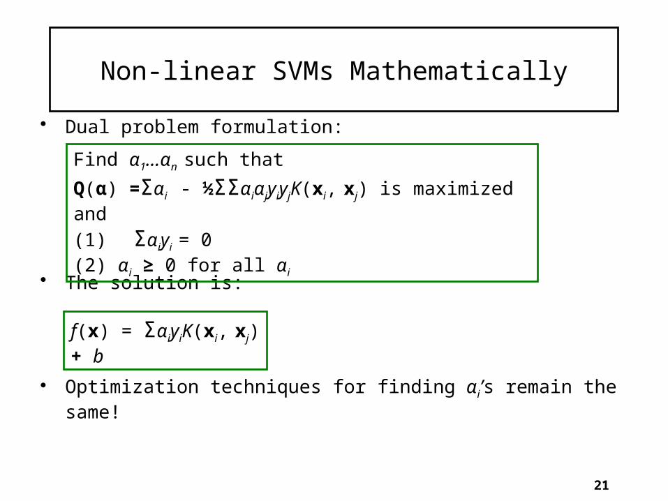
Non-linear SVMs Mathematically

• Dual problem formulation:

• The solution is:

• Optimization techniques for finding αi’s remain the same!

Find α1…αn such that

Q(α) =Σαi - ½ΣΣαiαjyiyjK(xi, xj) is maximized and

(1) Σαiyi = 0(2) αi ≥ 0 for all αi

f(x) = ΣαiyiK(xi, xj)+ b

G53MLE | Machine Learning | Dr Guoping Qiu

Unique Features of SVM’s and Kernel Methods

22

Are explicitly based on a theoretical model of learning

Come with theoretical guarantees about their performance

Have a modular design that allows one to separately implement and design their components

Are not affected by local minima

Do not suffer from the curse of dimensionality

G53MLE | Machine Learning | Dr Guoping Qiu

SVM Application Examples

23

Face detection

G53MLE | Machine Learning | Dr Guoping Qiu

SVM Software and Resources

24

http://www.svms.org/tutorials/

LIBSVM -- A Library for Support Vector Machines by Chih-Chung Chang and Chih-Jen Lin

http://www.csie.ntu.edu.tw/~cjlin/libsvm/