machine learning & mechanism design -...
TRANSCRIPT

Machine Learning & Mechanism Design:Dynamic and Discriminatory Pricing in Auctions
Jason D. HartlineMicrosoft Research – Silicon Valley
(Joint with with Maria-Florina Balcan,
Avrim Blum, and Yishay Mansour)
August 5, 2005
The Problem
Sellers can extract more of surplus with discriminatory pricing.
DISCRIMINATORY AUCTIONS – AUGUST 5, 20051
The Problem
Sellers can extract more of surplus with discriminatory pricing.
Two approaches:
1. Distinguish between products.(E.g., software versioning, airline tickets, etc.)
2. Price discriminate with observable customer features.(E.g., college tuition, DVDs, car insurance, shipping)
Goal: design mechanism to optimally price discriminate.
DISCRIMINATORY AUCTIONS – AUGUST 5, 20051

Optimal Mechanism Design
Typical Economic approach to optimal mechanism design:
• Assume valuations are from known distribution.
• Design optimal auction for distribution.
DISCRIMINATORY AUCTIONS – AUGUST 5, 20052

Optimal Mechanism Design
Typical Economic approach to optimal mechanism design:
• Assume valuations are from known distribution.
• Design optimal auction for distribution.
Notes on optimal mechanism design problem:
• Solved by Myerson (for single-parameter case).
• non-identical distributions =⇒ discriminatory pricing.
• Assumed known distribution ignores:
– incentives (of acquiring distribution)
– performance (from inaccurate distribution)
Goal: understand how quality and incentives of learning distributionaffect profit.
DISCRIMINATORY AUCTIONS – AUGUST 5, 20052

Setting
1. Unlimited supply of stuff to sell.
2. bidders with private valuations for stuff.
3. make each bidder an offer.
4. revenue is incentive compatible function of offer and valuation.
DISCRIMINATORY AUCTIONS – AUGUST 5, 20053

Setting
1. Unlimited supply of stuff to sell.(Example 1: MS Office Professional (PV) & Student Version (SV))
2. bidders with private valuations for stuff.
3. make each bidder an offer.
4. revenue is incentive compatible function of offer and valuation.
DISCRIMINATORY AUCTIONS – AUGUST 5, 20053
Setting
1. Unlimited supply of stuff to sell.(Example 1: MS Office Professional (PV) & Student Version (SV))
2. bidders with private valuations for stuff.(Example 1: Bidder: “PV worth $400, SV worth $300”)
3. make each bidder an offer.
4. revenue is incentive compatible function of offer and valuation.
DISCRIMINATORY AUCTIONS – AUGUST 5, 20053
Setting
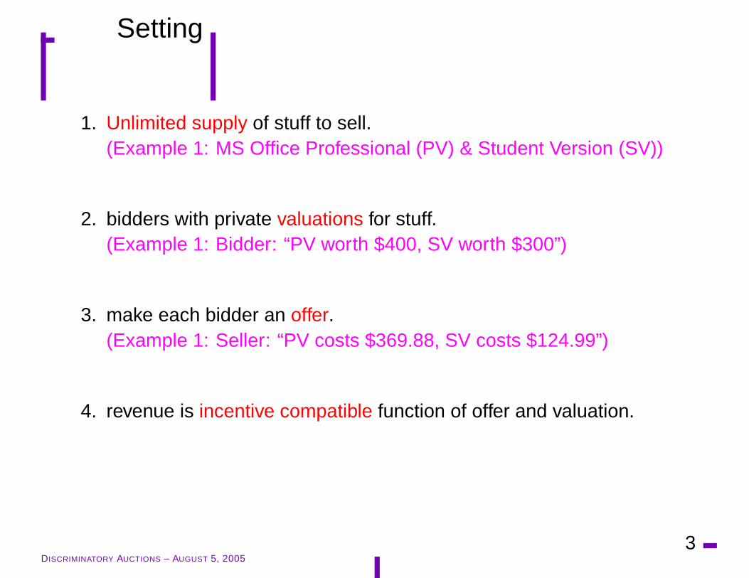
1. Unlimited supply of stuff to sell.(Example 1: MS Office Professional (PV) & Student Version (SV))
2. bidders with private valuations for stuff.(Example 1: Bidder: “PV worth $400, SV worth $300”)
3. make each bidder an offer.(Example 1: Seller: “PV costs $369.88, SV costs $124.99”)
4. revenue is incentive compatible function of offer and valuation.
DISCRIMINATORY AUCTIONS – AUGUST 5, 20053
Setting
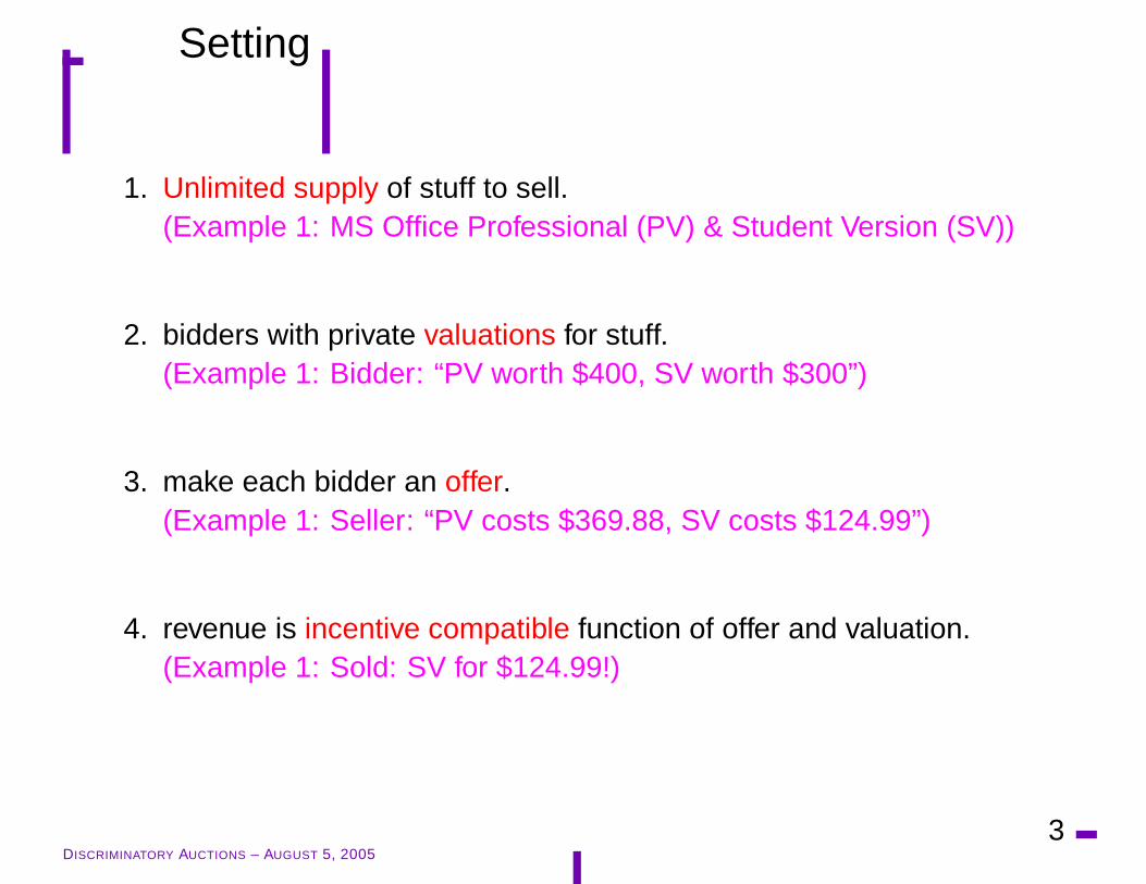
1. Unlimited supply of stuff to sell.(Example 1: MS Office Professional (PV) & Student Version (SV))
2. bidders with private valuations for stuff.(Example 1: Bidder: “PV worth $400, SV worth $300”)
3. make each bidder an offer.(Example 1: Seller: “PV costs $369.88, SV costs $124.99”)
4. revenue is incentive compatible function of offer and valuation.(Example 1: Sold: SV for $124.99!)
DISCRIMINATORY AUCTIONS – AUGUST 5, 20053
Setting
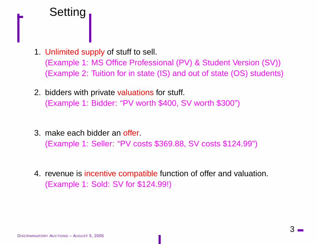
1. Unlimited supply of stuff to sell.(Example 1: MS Office Professional (PV) & Student Version (SV))(Example 2: Tuition for in state (IS) and out of state (OS) students)
2. bidders with private valuations for stuff.(Example 1: Bidder: “PV worth $400, SV worth $300”)
3. make each bidder an offer.(Example 1: Seller: “PV costs $369.88, SV costs $124.99”)
4. revenue is incentive compatible function of offer and valuation.(Example 1: Sold: SV for $124.99!)
DISCRIMINATORY AUCTIONS – AUGUST 5, 20053

Setting
1. Unlimited supply of stuff to sell.(Example 1: MS Office Professional (PV) & Student Version (SV))(Example 2: Tuition for in state (IS) and out of state (OS) students)
2. bidders with private valuations for stuff.(Example 1: Bidder: “PV worth $400, SV worth $300”)(Example 2: Bidder (OS): “Tuition worth $15,000”)
3. make each bidder an offer.(Example 1: Seller: “PV costs $369.88, SV costs $124.99”)(Example 2: Seller: “IS costs $9,256.80, OS costs $16,855.30,”)
4. revenue is incentive compatible function of offer and valuation.(Example 1: Sold: SV for $124.99!)(Example 2: No Sale!)
DISCRIMINATORY AUCTIONS – AUGUST 5, 20053

Overview
1.=⇒ Auction Problem
(a) Random Sampling Solution
(b) Retrospective bounds.
(c) Software Versioning Example.
2. Online Auction Problem
(a) Expert Learning based Auction.
(b) Expert Learning with non-uniform bounds.
3. Conclusions
DISCRIMINATORY AUCTIONS – AUGUST 5, 20054
Auction Problem
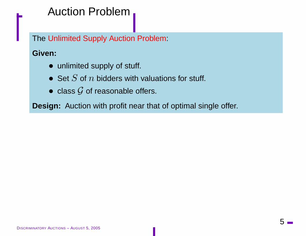
The Unlimited Supply Auction Problem:
Given:
• unlimited supply of stuff.
• Set S of n bidders with valuations for stuff.
• class G of reasonable offers.
Design: Auction with profit near that of optimal single offer.
DISCRIMINATORY AUCTIONS – AUGUST 5, 20055

Auction Problem
The Unlimited Supply Auction Problem:
Given:
• unlimited supply of stuff.
• Set S of n bidders with valuations for stuff.
• class G of reasonable offers.
Design: Auction with profit near that of optimal single offer.
Notation:
• g(i) = payoff from bidder i when offered g.
• g(S) =∑
i∈S g(i).
• optG(S) = argmaxg∈G g(S).
• OPTG(S) = maxg∈G g(S).
DISCRIMINATORY AUCTIONS – AUGUST 5, 20055
Random Sampling Auction
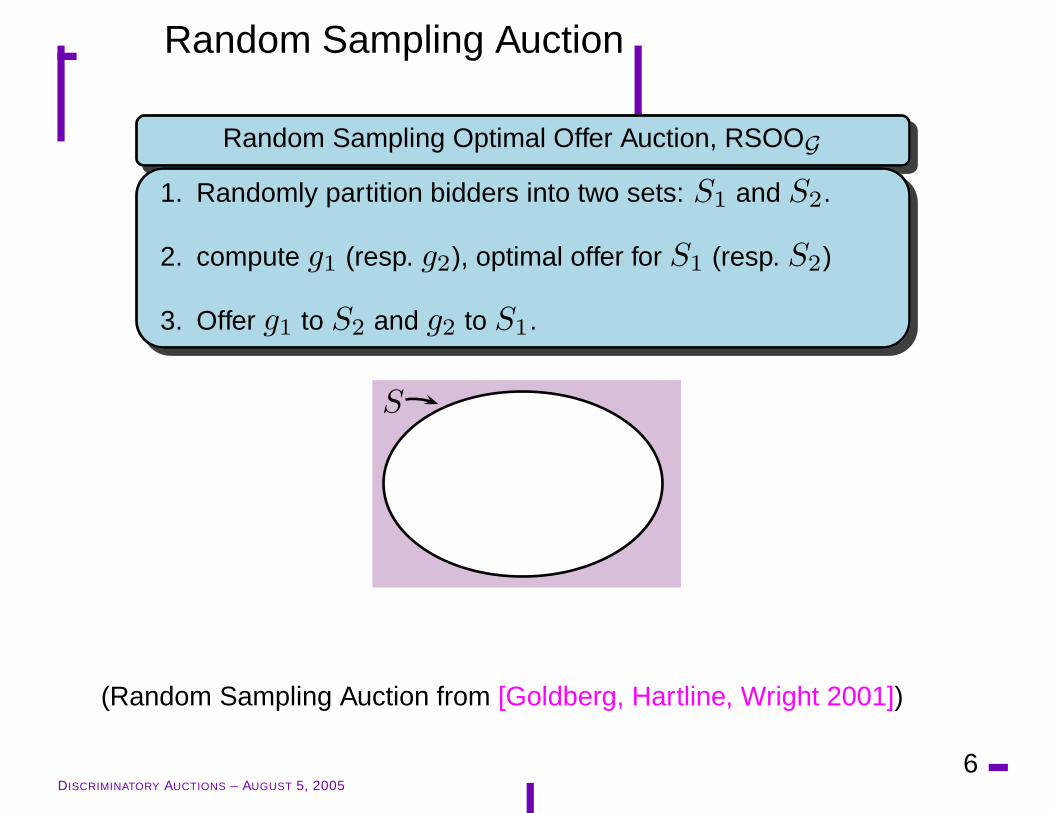
Random Sampling Optimal Offer Auction, RSOOG
1. Randomly partition bidders into two sets: S1 and S2.
2. compute g1 (resp. g2), optimal offer for S1 (resp. S2)
3. Offer g1 to S2 and g2 to S1.
S
(Random Sampling Auction from [Goldberg, Hartline, Wright 2001])
DISCRIMINATORY AUCTIONS – AUGUST 5, 20056

Random Sampling Auction
Random Sampling Optimal Offer Auction, RSOOG
1. Randomly partition bidders into two sets: S1 and S2.
2. compute g1 (resp. g2), optimal offer for S1 (resp. S2)
3. Offer g1 to S2 and g2 to S1.
SS1
S2
(Random Sampling Auction from [Goldberg, Hartline, Wright 2001])
DISCRIMINATORY AUCTIONS – AUGUST 5, 20056

Random Sampling Auction
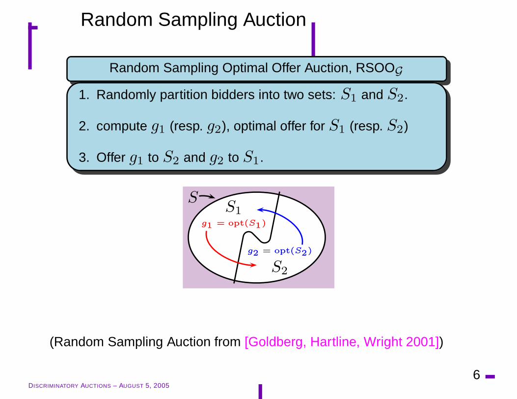
Random Sampling Optimal Offer Auction, RSOOG
1. Randomly partition bidders into two sets: S1 and S2.
2. compute g1 (resp. g2), optimal offer for S1 (resp. S2)
3. Offer g1 to S2 and g2 to S1.
SS1
S2
g1 = opt(S1)
g2 = opt(S2)
(Random Sampling Auction from [Goldberg, Hartline, Wright 2001])
DISCRIMINATORY AUCTIONS – AUGUST 5, 20056
Random Sampling Auction
Random Sampling Optimal Offer Auction, RSOOG
1. Randomly partition bidders into two sets: S1 and S2.
2. compute g1 (resp. g2), optimal offer for S1 (resp. S2)
3. Offer g1 to S2 and g2 to S1.
SS1
S2
g1 = opt(S1)
g2 = opt(S2)
g1 = opt(S1)
g2 = opt(S2)
(Random Sampling Auction from [Goldberg, Hartline, Wright 2001])
DISCRIMINATORY AUCTIONS – AUGUST 5, 20056

Random Sampling Auction
Random Sampling Optimal Offer Auction, RSOOG
1. Randomly partition bidders into two sets: S1 and S2.
2. compute g1 (resp. g2), optimal offer for S1 (resp. S2)
3. Offer g1 to S2 and g2 to S1.
SS1
S2
g1 = opt(S1)
g2 = opt(S2)
g1 = opt(S1)
g2 = opt(S2)
Question: when is RSOOG good?
(Random Sampling Auction from [Goldberg, Hartline, Wright 2001])
DISCRIMINATORY AUCTIONS – AUGUST 5, 20056
Performance Analysis
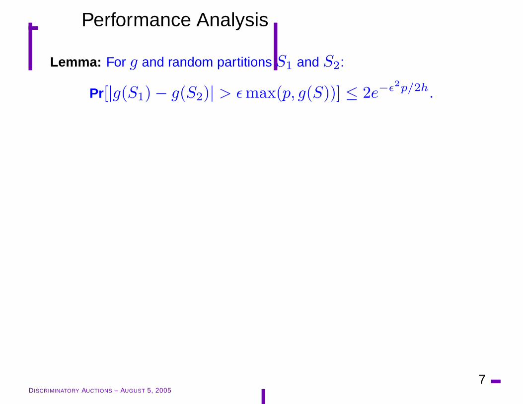
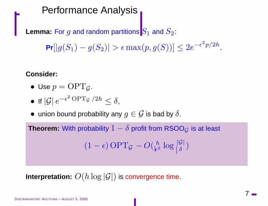
Lemma: For g and random partitions S1 and S2:
Pr[|g(S1) − g(S2)| > εmax(p, g(S))] ≤ 2e−ε2p/2h.
DISCRIMINATORY AUCTIONS – AUGUST 5, 20057
Performance Analysis
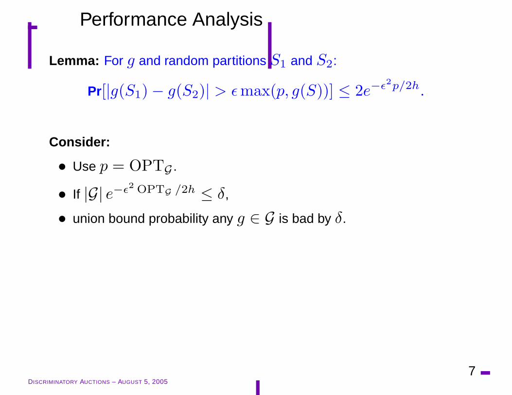
Lemma: For g and random partitions S1 and S2:
Pr[|g(S1) − g(S2)| > εmax(p, g(S))] ≤ 2e−ε2p/2h.
Consider:
• Use p = OPTG .
• If |G| e−ε2 OPTG /2h ≤ δ,
• union bound probability any g ∈ G is bad by δ.
DISCRIMINATORY AUCTIONS – AUGUST 5, 20057

Performance Analysis
Lemma: For g and random partitions S1 and S2:
Pr[|g(S1) − g(S2)| > εmax(p, g(S))] ≤ 2e−ε2p/2h.
Consider:
• Use p = OPTG .
• If |G| e−ε2 OPTG /2h ≤ δ,
• union bound probability any g ∈ G is bad by δ.
Theorem: With probability 1 − δ profit from RSOOG is at least
(1 − ε)OPTG −O( hε2 log |G|
δ )
DISCRIMINATORY AUCTIONS – AUGUST 5, 20057
Performance Analysis
Lemma: For g and random partitions S1 and S2:
Pr[|g(S1) − g(S2)| > εmax(p, g(S))] ≤ 2e−ε2p/2h.
Consider:
• Use p = OPTG .
• If |G| e−ε2 OPTG /2h ≤ δ,
• union bound probability any g ∈ G is bad by δ.
Theorem: With probability 1 − δ profit from RSOOG is at least
(1 − ε)OPTG −O( hε2 log |G|
δ )
Interpretation: O(h log |G|) is convergence time.
DISCRIMINATORY AUCTIONS – AUGUST 5, 20057

Example
Example: Selling tee shirts. (discretized prices)
• Bidders with valuations in [1, h] for a tee shirt.
• Reasonable offers: G = {price 2i for i ∈ {1, . . . , log h}}.
• Convergence Time: O(h log |G|) = O(h log log h)
DISCRIMINATORY AUCTIONS – AUGUST 5, 20058

Overview
1. Auction Problem
(a) Random Sampling Solution
(b)=⇒ Retrospective bounds.
(c) Software Versioning Example.
2. Online Auction Problem
(a) Expert Learning based Auction.
(b) Expert Learning with non-uniform bounds.
3. Conclusions
DISCRIMINATORY AUCTIONS – AUGUST 5, 20059

|G| = ∞?
What if |G| = ∞?
DISCRIMINATORY AUCTIONS – AUGUST 5, 200510

|G| = ∞?
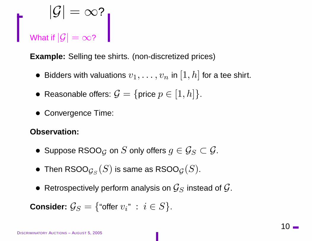
What if |G| = ∞?
Example: Selling tee shirts. (non-discretized prices)
• Bidders with valuations v1, . . . , vn in [1, h] for a tee shirt.
• Reasonable offers: G = {price p ∈ [1, h]}.
• Convergence Time:
DISCRIMINATORY AUCTIONS – AUGUST 5, 200510

|G| = ∞?
What if |G| = ∞?
Example: Selling tee shirts. (non-discretized prices)
• Bidders with valuations v1, . . . , vn in [1, h] for a tee shirt.
• Reasonable offers: G = {price p ∈ [1, h]}.
• Convergence Time:
Observation:
• Suppose RSOOG on S only offers g ∈ GS ⊂ G.
• Then RSOOGS(S) is same as RSOOG(S).
• Retrospectively perform analysis on GS instead of G.
DISCRIMINATORY AUCTIONS – AUGUST 5, 200510
|G| = ∞?
What if |G| = ∞?
Example: Selling tee shirts. (non-discretized prices)
• Bidders with valuations v1, . . . , vn in [1, h] for a tee shirt.
• Reasonable offers: G = {price p ∈ [1, h]}.
• Convergence Time:
Observation:
• Suppose RSOOG on S only offers g ∈ GS ⊂ G.
• Then RSOOGS(S) is same as RSOOG(S).
• Retrospectively perform analysis on GS instead of G.
Consider: GS = {“offer vi” : i ∈ S}.
DISCRIMINATORY AUCTIONS – AUGUST 5, 200510
|G| = ∞?
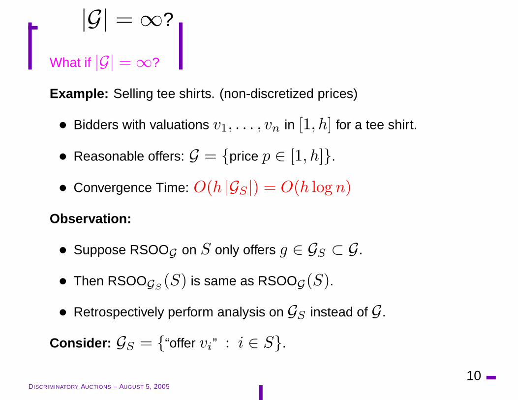
What if |G| = ∞?
Example: Selling tee shirts. (non-discretized prices)
• Bidders with valuations v1, . . . , vn in [1, h] for a tee shirt.
• Reasonable offers: G = {price p ∈ [1, h]}.
• Convergence Time: O(h |GS |) = O(h log n)
Observation:
• Suppose RSOOG on S only offers g ∈ GS ⊂ G.
• Then RSOOGS(S) is same as RSOOG(S).
• Retrospectively perform analysis on GS instead of G.
Consider: GS = {“offer vi” : i ∈ S}.
DISCRIMINATORY AUCTIONS – AUGUST 5, 200510

Example: Software Versioning
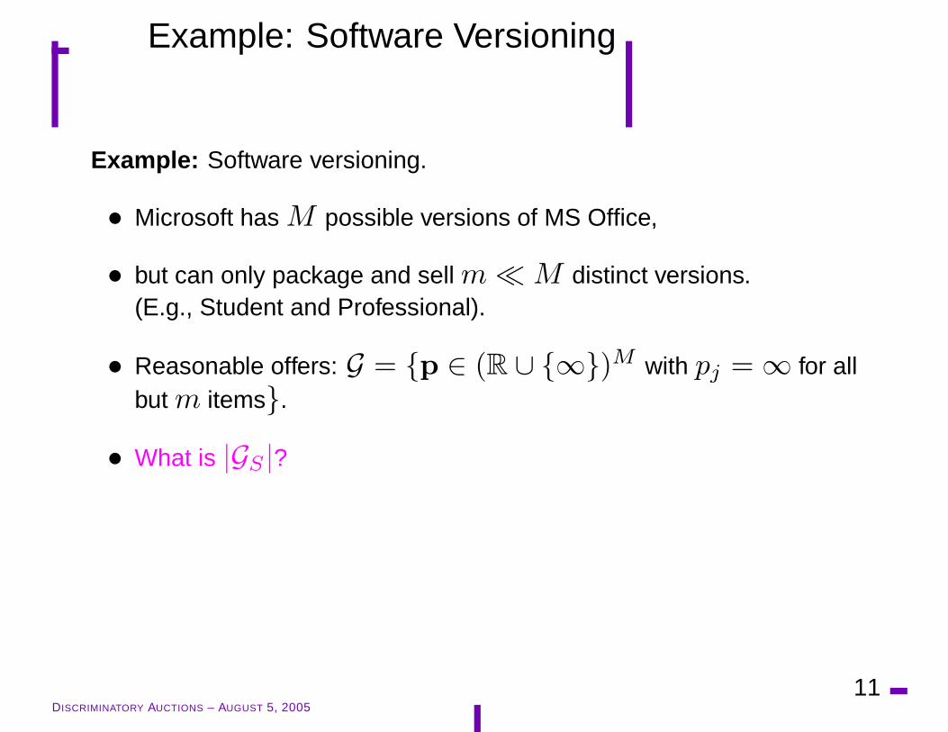
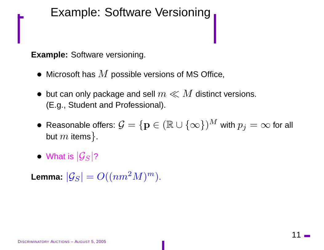
Example: Software versioning.
• Microsoft has M possible versions of MS Office,
• but can only package and sell m � M distinct versions.(E.g., Student and Professional).
DISCRIMINATORY AUCTIONS – AUGUST 5, 200511

Example: Software Versioning
Example: Software versioning.
• Microsoft has M possible versions of MS Office,
• but can only package and sell m � M distinct versions.(E.g., Student and Professional).
• Reasonable offers: G = {p ∈ (R ∪ {∞})M with pj = ∞ for allbut m items}.
DISCRIMINATORY AUCTIONS – AUGUST 5, 200511
Example: Software Versioning
Example: Software versioning.
• Microsoft has M possible versions of MS Office,
• but can only package and sell m � M distinct versions.(E.g., Student and Professional).
• Reasonable offers: G = {p ∈ (R ∪ {∞})M with pj = ∞ for allbut m items}.
• What is |GS |?
Lemma: |GS | = O((nm2M)m).
DISCRIMINATORY AUCTIONS – AUGUST 5, 200511

Example: Software Versioning
Example: Software versioning.
• Microsoft has M possible versions of MS Office,
• but can only package and sell m � M distinct versions.(E.g., Student and Professional).
• Reasonable offers: G = {p ∈ (R ∪ {∞})M with pj = ∞ for allbut m items}.
• What is |GS |?
Lemma: |GS | = O((nm2M)m).
Convergence time = O(hm log(nm2M)) .
DISCRIMINATORY AUCTIONS – AUGUST 5, 200511

Example: Software Versioning
Example: Software versioning.
• Microsoft has M possible versions of MS Office,
• but can only package and sell m � M distinct versions.(E.g., Student and Professional).
• Reasonable offers: G = {p ∈ (R ∪ {∞})M with pj = ∞ for allbut m items}.
• What is |GS |?
Lemma: |GS | = O((nm2M)m).
Convergence time = O(hm log(nm2M)) ≈ O(hm log n).
DISCRIMINATORY AUCTIONS – AUGUST 5, 200511

Proof of Lemma
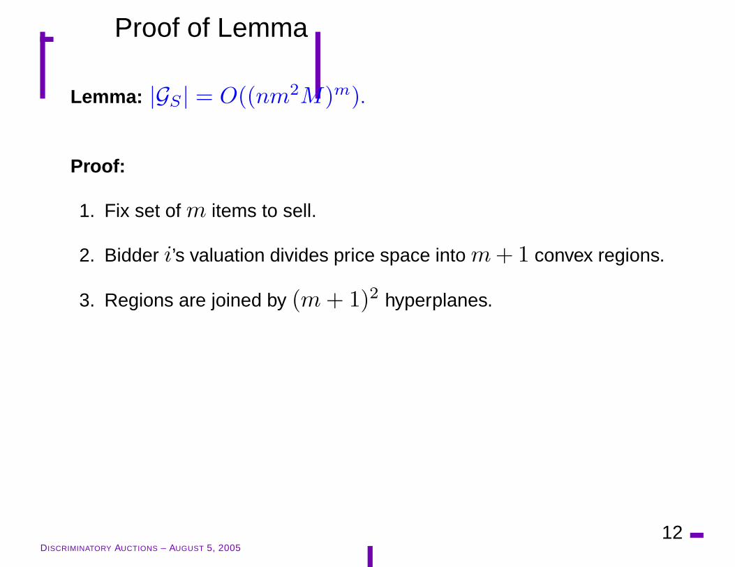
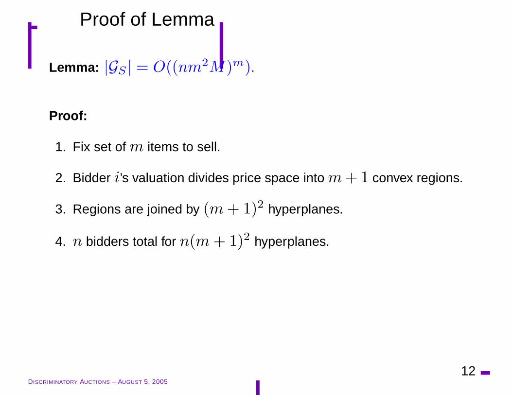
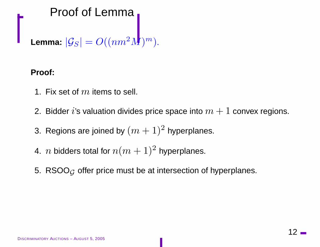
Lemma: |GS | = O((nm2M)m).
DISCRIMINATORY AUCTIONS – AUGUST 5, 200512

Proof of Lemma
Lemma: |GS | = O((nm2M)m).
Proof:
1. Fix set of m items to sell.
2. Bidder i’s valuation divides price space into m + 1 convex regions.
DISCRIMINATORY AUCTIONS – AUGUST 5, 200512
Proof of Lemma
Lemma: |GS | = O((nm2M)m).
Proof:
1. Fix set of m items to sell.
2. Bidder i’s valuation divides price space into m + 1 convex regions.
3. Regions are joined by (m + 1)2 hyperplanes.
DISCRIMINATORY AUCTIONS – AUGUST 5, 200512
Proof of Lemma
Lemma: |GS | = O((nm2M)m).
Proof:
1. Fix set of m items to sell.
2. Bidder i’s valuation divides price space into m + 1 convex regions.
3. Regions are joined by (m + 1)2 hyperplanes.
4. n bidders total for n(m + 1)2 hyperplanes.
DISCRIMINATORY AUCTIONS – AUGUST 5, 200512
Proof of Lemma
Lemma: |GS | = O((nm2M)m).
Proof:
1. Fix set of m items to sell.
2. Bidder i’s valuation divides price space into m + 1 convex regions.
3. Regions are joined by (m + 1)2 hyperplanes.
4. n bidders total for n(m + 1)2 hyperplanes.
5. RSOOG offer price must be at intersection of hyperplanes.
DISCRIMINATORY AUCTIONS – AUGUST 5, 200512

Proof of Lemma
Lemma: |GS | = O((nm2M)m).
Proof:
1. Fix set of m items to sell.
2. Bidder i’s valuation divides price space into m + 1 convex regions.
3. Regions are joined by (m + 1)2 hyperplanes.
4. n bidders total for n(m + 1)2 hyperplanes.
5. RSOOG offer price must be at intersection of hyperplanes.
6. K = n(m + 1)2 hyperplanes in m dimensions intersect in Km.
7. Sum over Mm possible m-item sets.
DISCRIMINATORY AUCTIONS – AUGUST 5, 200512
Other Results
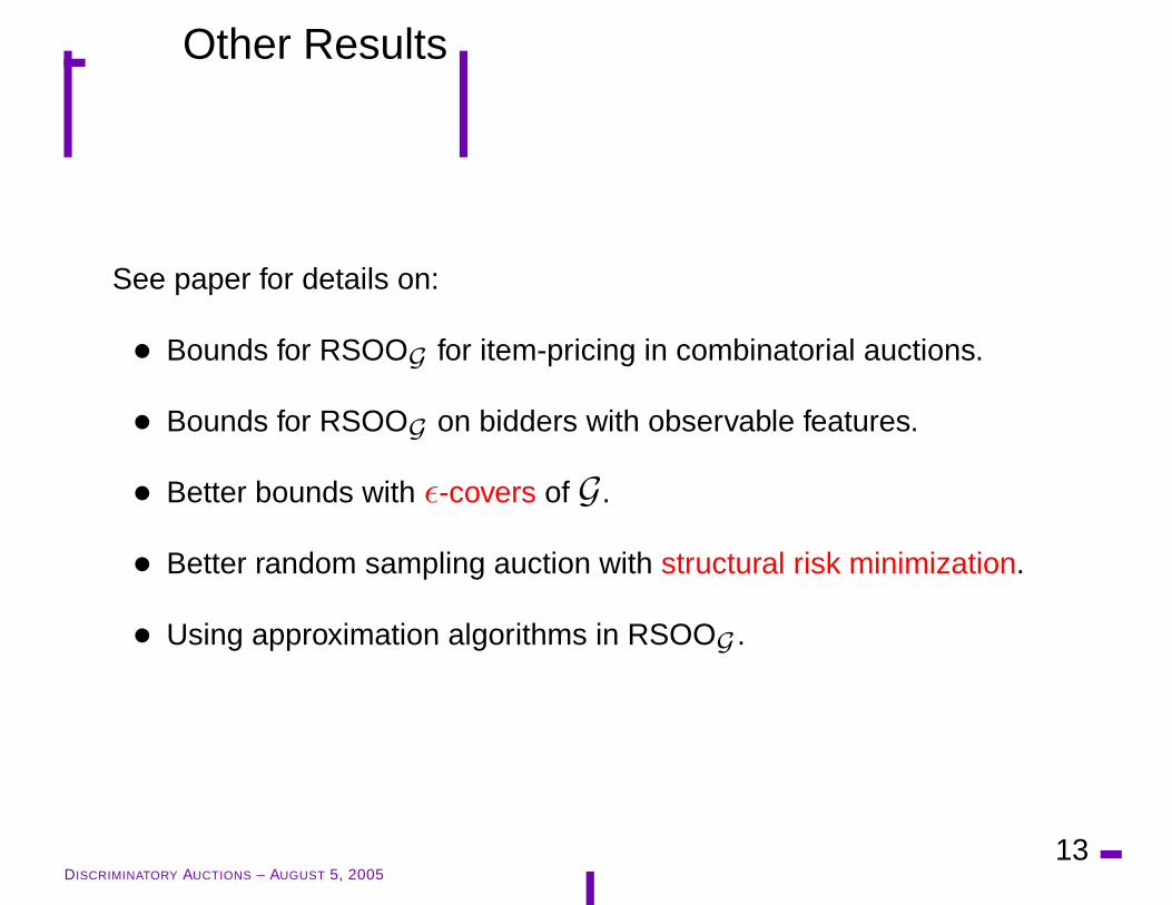
See paper for details on:
• Bounds for RSOOG for item-pricing in combinatorial auctions.
• Bounds for RSOOG on bidders with observable features.
• Better bounds with ε-covers of G.
• Better random sampling auction with structural risk minimization.
• Using approximation algorithms in RSOOG .
DISCRIMINATORY AUCTIONS – AUGUST 5, 200513

Overview
1. Auction Problem
(a) Random Sampling Solution
(b) Retrospective bounds.
(c) Software Versioning Example.
2.=⇒ Online Auction Problem
(a) Expert Learning based Auction.
(b) Expert Learning with non-uniform bounds.
3. Conclusions
DISCRIMINATORY AUCTIONS – AUGUST 5, 200514

Online Auction Problem
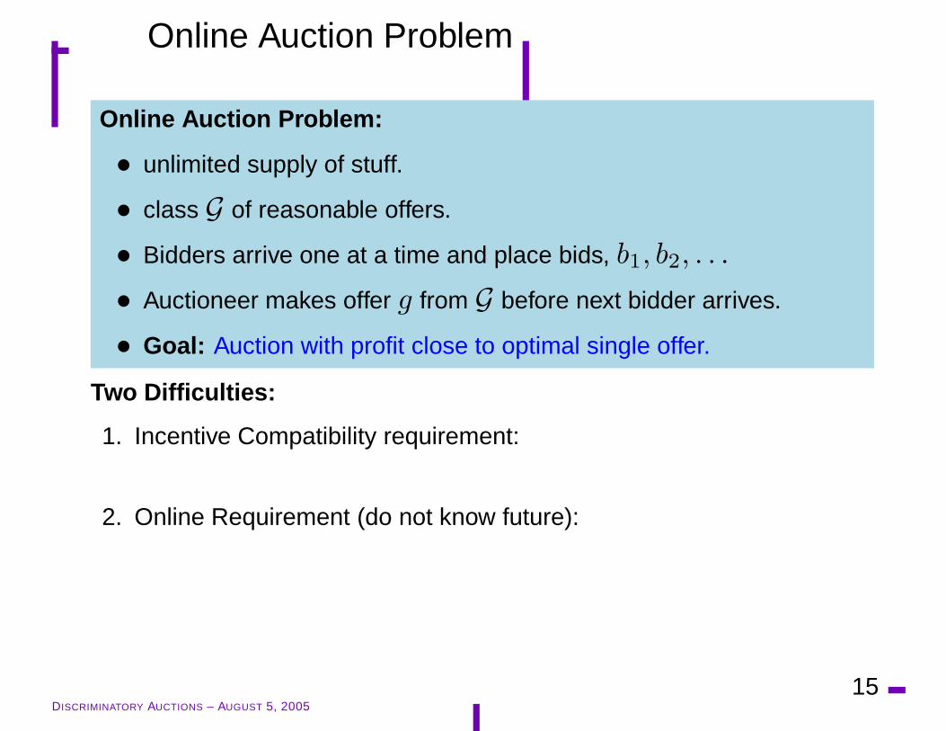
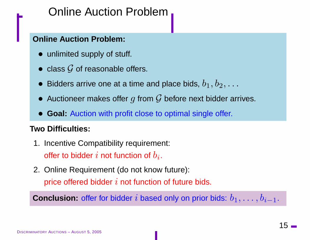
Online Auction Problem:
• unlimited supply of stuff.
• class G of reasonable offers.
• Bidders arrive one at a time and place bids, b1, b2, . . .
• Auctioneer makes offer g from G before next bidder arrives.
• Goal: Auction with profit close to optimal single offer.
DISCRIMINATORY AUCTIONS – AUGUST 5, 200515
Online Auction Problem
Online Auction Problem:
• unlimited supply of stuff.
• class G of reasonable offers.
• Bidders arrive one at a time and place bids, b1, b2, . . .
• Auctioneer makes offer g from G before next bidder arrives.
• Goal: Auction with profit close to optimal single offer.
Two Difficulties:
1. Incentive Compatibility requirement:
2. Online Requirement (do not know future):
DISCRIMINATORY AUCTIONS – AUGUST 5, 200515

Online Auction Problem
Online Auction Problem:
• unlimited supply of stuff.
• class G of reasonable offers.
• Bidders arrive one at a time and place bids, b1, b2, . . .
• Auctioneer makes offer g from G before next bidder arrives.
• Goal: Auction with profit close to optimal single offer.
Two Difficulties:
1. Incentive Compatibility requirement:
offer to bidder i not function of bi.
2. Online Requirement (do not know future):
price offered bidder i not function of future bids.
DISCRIMINATORY AUCTIONS – AUGUST 5, 200515
Online Auction Problem
Online Auction Problem:
• unlimited supply of stuff.
• class G of reasonable offers.
• Bidders arrive one at a time and place bids, b1, b2, . . .
• Auctioneer makes offer g from G before next bidder arrives.
• Goal: Auction with profit close to optimal single offer.
Two Difficulties:
1. Incentive Compatibility requirement:
offer to bidder i not function of bi.
2. Online Requirement (do not know future):
price offered bidder i not function of future bids.
Conclusion: offer for bidder i based only on prior bids: b1, . . . , bi−1.
DISCRIMINATORY AUCTIONS – AUGUST 5, 200515
Assumptions
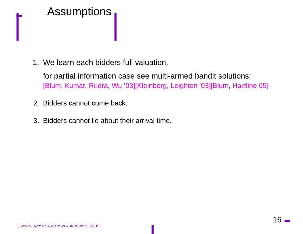
1. We learn each bidders full valuation.
DISCRIMINATORY AUCTIONS – AUGUST 5, 200516

Assumptions
1. We learn each bidders full valuation.
for partial information case see multi-armed bandit solutions:[Blum, Kumar, Rudra, Wu ’03][Kleinberg, Leighton ’03][Blum, Hartline 05]
DISCRIMINATORY AUCTIONS – AUGUST 5, 200516
Assumptions
1. We learn each bidders full valuation.
for partial information case see multi-armed bandit solutions:[Blum, Kumar, Rudra, Wu ’03][Kleinberg, Leighton ’03][Blum, Hartline 05]
2. Bidders cannot come back.
3. Bidders cannot lie about their arrival time.
DISCRIMINATORY AUCTIONS – AUGUST 5, 200516

Assumptions
1. We learn each bidders full valuation.
for partial information case see multi-armed bandit solutions:[Blum, Kumar, Rudra, Wu ’03][Kleinberg, Leighton ’03][Blum, Hartline 05]
2. Bidders cannot come back.
3. Bidders cannot lie about their arrival time.
for temporal strategyproofness see: [Hajiaghayi, Kleinberg, Parkes ’04]
DISCRIMINATORY AUCTIONS – AUGUST 5, 200516
Assumptions
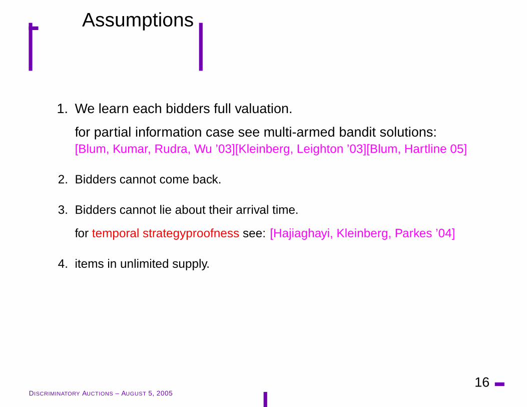
1. We learn each bidders full valuation.
for partial information case see multi-armed bandit solutions:[Blum, Kumar, Rudra, Wu ’03][Kleinberg, Leighton ’03][Blum, Hartline 05]
2. Bidders cannot come back.
3. Bidders cannot lie about their arrival time.
for temporal strategyproofness see: [Hajiaghayi, Kleinberg, Parkes ’04]
4. items in unlimited supply.
DISCRIMINATORY AUCTIONS – AUGUST 5, 200516
Assumptions
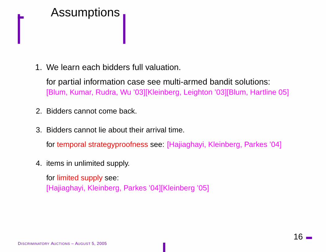
1. We learn each bidders full valuation.
for partial information case see multi-armed bandit solutions:[Blum, Kumar, Rudra, Wu ’03][Kleinberg, Leighton ’03][Blum, Hartline 05]
2. Bidders cannot come back.
3. Bidders cannot lie about their arrival time.
for temporal strategyproofness see: [Hajiaghayi, Kleinberg, Parkes ’04]
4. items in unlimited supply.
for limited supply see:[Hajiaghayi, Kleinberg, Parkes ’04][Kleinberg ’05]
DISCRIMINATORY AUCTIONS – AUGUST 5, 200516
Online Learning
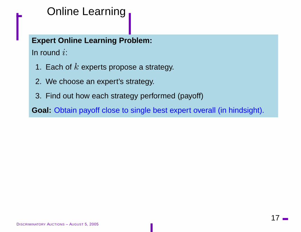
Expert Online Learning Problem:
In round i:
1. Each of k experts propose a strategy.
2. We choose an expert’s strategy.
3. Find out how each strategy performed (payoff)
Goal: Obtain payoff close to single best expert overall (in hindsight).
DISCRIMINATORY AUCTIONS – AUGUST 5, 200517

Online Learning
Expert Online Learning Problem:
In round i:
1. Each of k experts propose a strategy.
2. We choose an expert’s strategy.
3. Find out how each strategy performed (payoff)
Goal: Obtain payoff close to single best expert overall (in hindsight).
Weighted Majority Algorithm: (for round i)
Let h be maximum payoff. For expert j, let sj be total payoff thus far.
Choose expert j ’s strategy with probability proportional to (1+2ε)sj/h.
Result: E[payoff] = (1 − ε)OPT− h2ε log k.
DISCRIMINATORY AUCTIONS – AUGUST 5, 200517
Application to Online Auctions
Application: (to online auctions) [Blum Kumar Rudra Wu 2003]
DISCRIMINATORY AUCTIONS – AUGUST 5, 200518
Application to Online Auctions
Application: (to online auctions) [Blum Kumar Rudra Wu 2003]
1. Expert for each g ∈ G
DISCRIMINATORY AUCTIONS – AUGUST 5, 200518
Application to Online Auctions
Application: (to online auctions) [Blum Kumar Rudra Wu 2003]
1. Expert for each g ∈ G
2. Best expert ⇒ best offer.
DISCRIMINATORY AUCTIONS – AUGUST 5, 200518
Application to Online Auctions
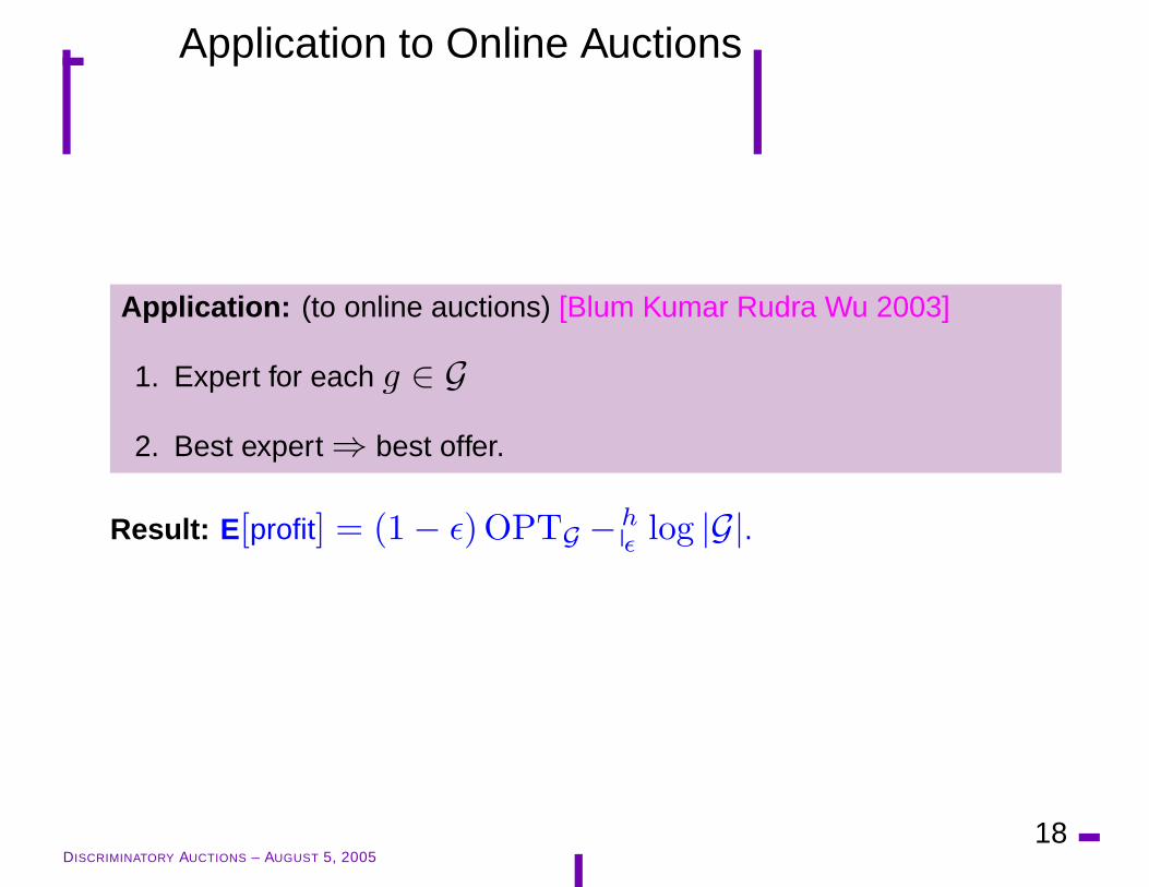
Application: (to online auctions) [Blum Kumar Rudra Wu 2003]
1. Expert for each g ∈ G
2. Best expert ⇒ best offer.
Result: E[profit] = (1 − ε)OPTG −hε log |G|.
DISCRIMINATORY AUCTIONS – AUGUST 5, 200518

Application to Online Auctions
Application: (to online auctions) [Blum Kumar Rudra Wu 2003]
1. Expert for each g ∈ G
2. Best expert ⇒ best offer.
Result: E[profit] = (1 − ε)OPTG −hε log |G|.
Note: Same convergence time as for RSOOG .
DISCRIMINATORY AUCTIONS – AUGUST 5, 200518
Example
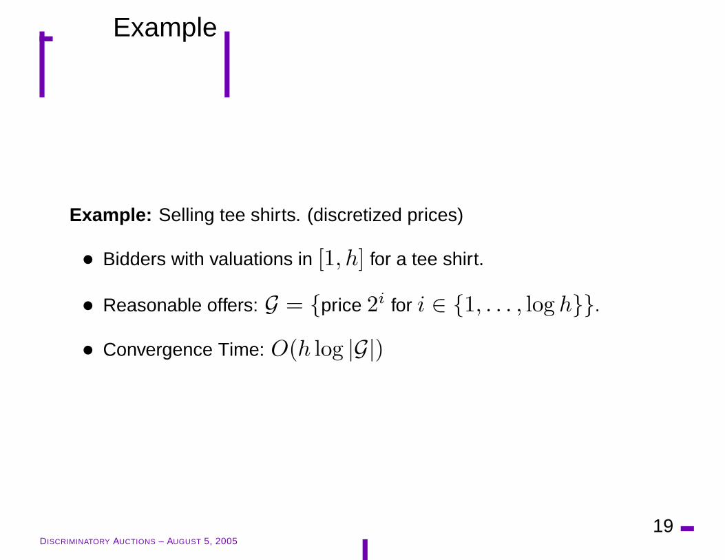
Example: Selling tee shirts. (discretized prices)
• Bidders with valuations in [1, h] for a tee shirt.
• Reasonable offers: G = {price 2i for i ∈ {1, . . . , log h}}.
• Convergence Time: O(h log |G|)
DISCRIMINATORY AUCTIONS – AUGUST 5, 200519
Example
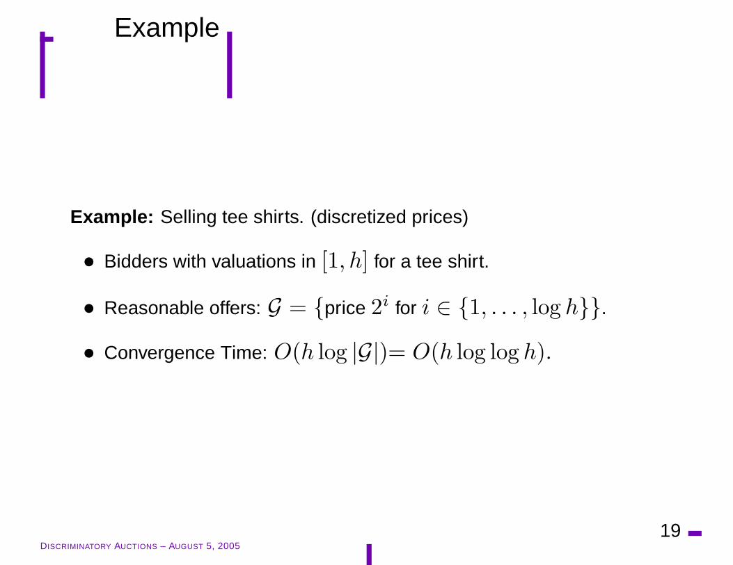
Example: Selling tee shirts. (discretized prices)
• Bidders with valuations in [1, h] for a tee shirt.
• Reasonable offers: G = {price 2i for i ∈ {1, . . . , log h}}.
• Convergence Time: O(h log |G|)= O(h log log h).
DISCRIMINATORY AUCTIONS – AUGUST 5, 200519
Better Bounds?
Can we get better bounds?
Retrospective technique like using GS does not work.
DISCRIMINATORY AUCTIONS – AUGUST 5, 200520

Overview
1. Auction Problem
(a) Random Sampling Solution
(b) Retrospective bounds.
(c) Software Versioning Example.
2. Online Auction Problem
(a) Expert Learning based Auction.
(b)=⇒ Expert Learning with non-uniform bounds.
3. Conclusions
DISCRIMINATORY AUCTIONS – AUGUST 5, 200521

Non-uniform Bounds on Payoff
Expert Online Learning Problem: In round i:
1. Each of k experts propose a strategy.
2. We choose an expert’s strategy.
3. Find out how each strategy performed (payoff)
4. Expert i’s payoff is always less than hi.
Goal: Obtain payoff close to single best expert overall (in hindsight).
DISCRIMINATORY AUCTIONS – AUGUST 5, 200522

Non-uniform Bounds on Payoff
Expert Online Learning Problem: In round i:
1. Each of k experts propose a strategy.
2. We choose an expert’s strategy.
3. Find out how each strategy performed (payoff)
4. Expert i’s payoff is always less than hi.
Goal: Obtain payoff close to single best expert overall (in hindsight).
Non-uniform Experts Algorithm: [Kalai ’01][Blum, Hartline ’05]
1. (initialization) For each expert, j, add initial score, sj , as:
hi × number of heads flipped in a row.
2. Run deterministic “go with best expert” algorithm.
Result: E[profit] ≥ OPT /2 −∑
i hi.
DISCRIMINATORY AUCTIONS – AUGUST 5, 200522

Application to Online Auctions
Application: (to online auctions)
DISCRIMINATORY AUCTIONS – AUGUST 5, 200523

Application to Online Auctions
Application: (to online auctions)
1. Bound hg for each g ∈ G.
2. Expert for each g ∈ G
3. Best expert ⇒ best offer.
DISCRIMINATORY AUCTIONS – AUGUST 5, 200523

Application to Online Auctions
Application: (to online auctions)
1. Bound hg for each g ∈ G.
2. Expert for each g ∈ G
3. Best expert ⇒ best offer.
Result: E[profit] = OPTG /2 −∑
g∈G hg .
DISCRIMINATORY AUCTIONS – AUGUST 5, 200523

Application to Online Auctions
Application: (to online auctions)
1. Bound hg for each g ∈ G.
2. Expert for each g ∈ G
3. Best expert ⇒ best offer.
Result: E[profit] = OPTG /2 −∑
g∈G hg .
Note: Convergence time =∑
g∈G hg
DISCRIMINATORY AUCTIONS – AUGUST 5, 200523
Example
Example: Selling tee shirts. (discretized prices)
• Bidders with valuations in [1, h] for a tee shirt.
• Reasonable offers: G = {price 2i for i ∈ {1, . . . , log h}}.
• Convergence Time:∑
g∈G hg .
DISCRIMINATORY AUCTIONS – AUGUST 5, 200524

Example
Example: Selling tee shirts. (discretized prices)
• Bidders with valuations in [1, h] for a tee shirt.
• Reasonable offers: G = {price 2i for i ∈ {1, . . . , log h}}.
• Convergence Time:∑
g∈G hg =∑log h
i 2i .
DISCRIMINATORY AUCTIONS – AUGUST 5, 200524

Example
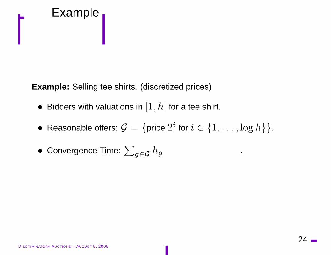
Example: Selling tee shirts. (discretized prices)
• Bidders with valuations in [1, h] for a tee shirt.
• Reasonable offers: G = {price 2i for i ∈ {1, . . . , log h}}.
• Convergence Time:∑
g∈G hg =∑log h
i 2i ≤ 2h.
DISCRIMINATORY AUCTIONS – AUGUST 5, 200524

Example
Example: Selling tee shirts. (discretized prices)
• Bidders with valuations in [1, h] for a tee shirt.
• Reasonable offers: G = {price 2i for i ∈ {1, . . . , log h}}.
• Convergence Time:∑
g∈G hg =∑log h
i 2i ≤ 2h.
Note: this is optimal up to constant factors.
DISCRIMINATORY AUCTIONS – AUGUST 5, 200524
Conclusions
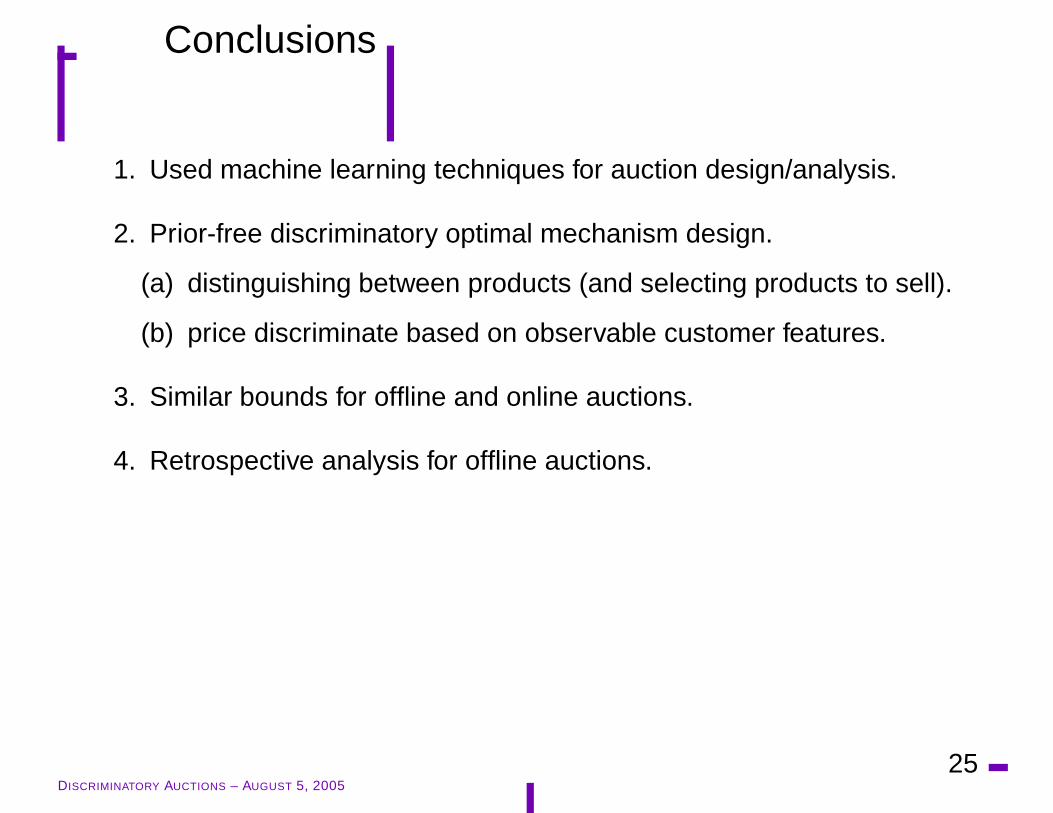
1. Used machine learning techniques for auction design/analysis.
2. Prior-free discriminatory optimal mechanism design.
(a) distinguishing between products (and selecting products to sell).
(b) price discriminate based on observable customer features.
3. Similar bounds for offline and online auctions.
4. Retrospective analysis for offline auctions.
DISCRIMINATORY AUCTIONS – AUGUST 5, 200525
Conclusions
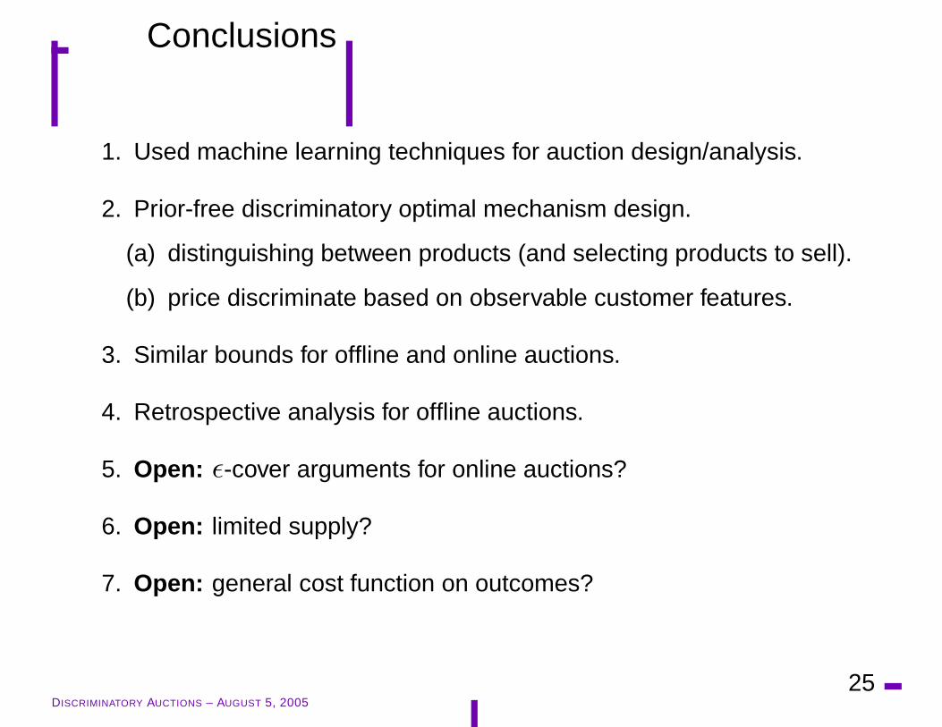
1. Used machine learning techniques for auction design/analysis.
2. Prior-free discriminatory optimal mechanism design.
(a) distinguishing between products (and selecting products to sell).
(b) price discriminate based on observable customer features.
3. Similar bounds for offline and online auctions.
4. Retrospective analysis for offline auctions.
5. Open: ε-cover arguments for online auctions?
6. Open: limited supply?
7. Open: general cost function on outcomes?
DISCRIMINATORY AUCTIONS – AUGUST 5, 200525