Machine Learning Methods for Demosaicing and Denoising

Yu-Sheng ChenStanford University

Computational and Mathematical Engineeringyusheng@stanford.edu

Stephanie SanchezStanford University

Computational and Mathematical Engineeringssanche2@stanford.edu

Abstract

We have implemented super-resolution techniques suchas machine learning methods and solving a least squaresproblem with a prior to perform demosaicing. These tech-niques include k-nearest neighbors (KNN), linear regres-sion, and alternating direction method of multipliers with atotal variation prior (ADMM TV). For all methods, param-eters were optimized to minimize the mean-squared-error(MSE) and maximize the peak signal-to-noise ratio (PSNR).The MSE and PSNR were compared to the results of tradi-tional demosaicing methods, bilinear and Malvar interpo-lation.

1. Introduction1.1. Motivation

If we consider demosaicing and super-resolution to-gether we notice that both methods utilize a technique tofill in pixel value information. Therefore, we have imple-mented a method that utilizes super-resolution techniquessuch as machine learning methods and solving a leastsquares problem to perform demosaicing.

1.2. Related Work

Traditional demosaicing methods include bilinear andMalvar interpolation. Bilinear interpolation approximatespixel values by averaging known pixel values in differentdirections. Malvar uses only linear kernels to perform thedemosaicing by optimizing the kernel gain parameters [3].

There are many machine learning methods for imagesuper-resolution [4], for example, k-Nearest Neighbors,Support Vector Regression and Super-Resolution Convo-lutional Neural Network. Machine learning techniquesare used to predict the missing color/texture information.In the general image optimization problem, we modelthe problem as an optimization problem[5][6]. As men-tioned in [5], image optimization problems contain (1) avariable which represents the target image to be recon-

structed, (2) a linear operation matrix which represents thedownsampling/demosaicing process, (3) a penalty measurewhich represents the difference of the results of downsam-pling/demosaicing from the measured data, and (4) the pri-ors and constraints on the the variables. Usually we encodethe prior information as a penalty (regularization) term inthe objective function, to manage the ill-conditionedness ofthe original reconstruction problem. Once we define theconstrained optimization problem, iterative update methodsare applied to solve the best estimate of the higher resolu-tion image.

2. The Method2.1. Bayer Pattern Extraction and Noise

The first step in our procedure is to extract the bayer pat-tern from the image. We also note that the standard meth-ods for demosaicing, as well as ADMM+TV, kNN, and lin-ear regression, are also denoising methods. Therefore, weadded a small amount of noise to the bayered image withparameter σ = 0.01. An example is shown in Figure 1.

Figure 1. Bayer pattern with noise (noise parameter σ = 0.01).

2.2. Alternating Direction Method of Multipliersand Total Variation

The first method of our model solves a least squaresproblem to perform demosaicing. A classical approach forsolving a least squares problem is to apply Alternating Di-rection Method of Multipliers (ADMM) with a Total Varia-tion (TV) prior. This method promotes the usage of break-

1

ing apart the original problem into smaller subproblemsand solving them by employing proximal operators. Fig-ures 2 and 3 show the algorithm and proximal operators forADMM+TV, respectively. ADMM+TV was applied to eachcolor channel and in order to keep ”matrix-free” operations,function handles forAx andATx were created to return thebayer pattern of the approximated color channel at each it-eration.

Figure 2. ADMM with TV prior algorithm.

Figure 3. Proximal operators for ADMM with TV prior.

2.3. k-Nearest Neighbors

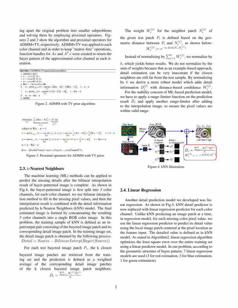
The machine learning (ML) methods can be applied topredict the missing details after the bilinear interpolationresult of bayer-patterned image is complete. As shown inFig.4, the bayer-patterned image is first split into 3 colorchannels, for each color channel, we use bilinear interpola-tion method to fill in the missing pixel values, and then theinterpolation result is combined with the detail informationpredicted by k-Nearest Neighbors (kNN) model. The finalestimated image is formed by concatenating the resulting3 color channels into a single RGB color image. In thisproblem, the training sample of kNN is defined as an in-put/output pair consisting of the bayered image patch and itscorresponding detail image patch. In the training image set,the detail image patch is obtained by the following process:Detail = Source−BilinearInterp(Bayer(Source))

For each test bayered image patch Pi, the k closest

bayered image patches are retrieved from the train-ing set and the prediction is defined as a weightedaverage of the corresponding detail image patchesof the k closest bayered image patch neighbors:

D̂i =∑k

j=1W(j)i D

(j)i

k

The weight W(j)i for the neighbor patch N

(j)i of

the given test patch Pi is defined based on the geo-metric distance between Pi and N

(j)i , as shown below:

W(j)i := e−α·dist(Pi,N

(j)i )

Instead of normalizing by∑kj=1W

(j)i , we normalize by

k, which yields better results. We do not normalize by thesum of weights because that as an example-based approach,detail estimation can be very inaccurate if the closestneighbors are still far from the test sample. By normalizingby k we derive a more robust model which adds detailinformation D

(j)i with distance-based confidence W

(j)i .

For the stability concern of ML-based prediction model,we have to apply a range-limiter function on the predictionresult D̂i and apply another range-limiter after addingto the interpolation image, to ensure the pixel values arewithin valid range.

Figure 4. kNN illustration.

2.4. Linear Regression

Another detail prediction model we developed was lin-ear regression. As shown in Fig.5, kNN detail predictor isnow replaced with linear regression predictor for each colorchannel. Unlike kNN predicting an image patch at a time,in regression model, for each missing color pixel value, weuse the linear regression predictor to predict its detail valueusing the local image patch centered at the pixel location asthe feature input. The detailed value is defined as in kNNmodel. As stated in Algorithm2, linear regression algorithmoptimizes the least square error over the entire training setusing a linear predictor model. In our problem, according tothe geometric structure of bayer pattern, 7 linear regressionmodels are used (3 for red estimation, 3 for blue estimation,1 for green estimation).

2

Figure 5. Regression illustration.

Data: training set {x(i), y(i)} for i=1,...,N , where Nis the number of training samples, x(i) ∈ Rkand y ∈ R

Result: optimal linear predictor hθ(x) := θTxbegin

minimize the cost function to obtain the optimal θ̂:

θ̂ := argminθ

1

2

N∑i=1

(hθ(x(i))− y(i))2

A. Iterative solution (Stochastic GradientDescent):

1 while until the cost converges do2 while i = 1, ..., N do

θ := θ + α(y(i) − hθ(x(i)))x(i)end

end

B. Batch solution (closed form):θ̂ = (XTX)−1XTYwhere

X :=

. . . (x(1))T . . .. . . (x(2))T . . .

.. . . (x(N))T . . .

, Y :=

y(1)

x(2)

.x(N)

end

Algorithm 1: Linear Regression Algorithm

3. Parameter Search

3.1. Parameter Optimization and Time Complexity

ADMM+TV, kNN, and linear regression are parametermethods. This means for ADMM+TV λ varies, and wevary patch sizes in kNN and regression. We optimized theparameters for the 24 images in the Kodak set so that themean-squared error (MSE) would be minimized and thepeak signal-to-noise ratio (PSNR) would be maximized.

A grid search was performed over 6 images of theKodak set to find an optimal λ that would minimize the

MSE over all 24 images. The time complexity to performthe gird search with 5 λ’s over 6 images was approximately6 hours. Even with performing grid search over 6 images,we found that the smallest λ provided the smallest MSE.Figures 6, 7, and 8 display this observation.

Figure 6. λ value search for Kodak image 4.

Figure 7. λ value search for Kodak image 19.

Figure 8. λ value search for Kodak image 23.

For the kNN method, the parameter k (number of closestneighbors for prediction) and image patch size are deter-mined by minimizing the MSE. As we can see in Fig.9,as k value increases, the MSE of test set decreases, be-cause the kNN model becomes more generalized to futuredata with larger k value. To the contrary, the MSE is evenhigher than the bilinear interpolation result when k = 3,which implies incorporating kNN detail prediction actuallydegrades the image quality. Additionally, the kNN com-putational complexity increases when k increases. This

3

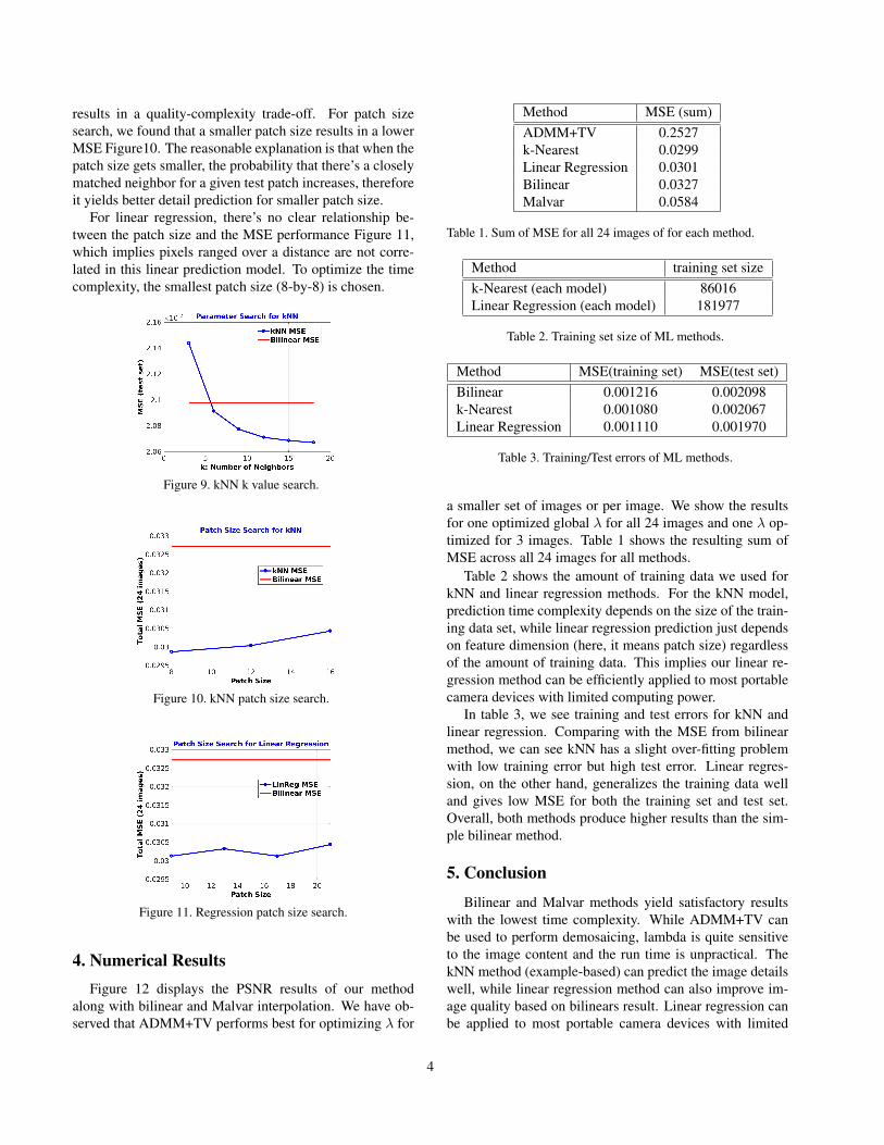
results in a quality-complexity trade-off. For patch sizesearch, we found that a smaller patch size results in a lowerMSE Figure10. The reasonable explanation is that when thepatch size gets smaller, the probability that there’s a closelymatched neighbor for a given test patch increases, thereforeit yields better detail prediction for smaller patch size.

For linear regression, there’s no clear relationship be-tween the patch size and the MSE performance Figure 11,which implies pixels ranged over a distance are not corre-lated in this linear prediction model. To optimize the timecomplexity, the smallest patch size (8-by-8) is chosen.

Figure 9. kNN k value search.

Figure 10. kNN patch size search.

Figure 11. Regression patch size search.

4. Numerical ResultsFigure 12 displays the PSNR results of our method

along with bilinear and Malvar interpolation. We have ob-served that ADMM+TV performs best for optimizing λ for

Method MSE (sum)ADMM+TV 0.2527k-Nearest 0.0299Linear Regression 0.0301Bilinear 0.0327Malvar 0.0584

Table 1. Sum of MSE for all 24 images of for each method.

Method training set sizek-Nearest (each model) 86016Linear Regression (each model) 181977

Table 2. Training set size of ML methods.

Method MSE(training set) MSE(test set)Bilinear 0.001216 0.002098k-Nearest 0.001080 0.002067Linear Regression 0.001110 0.001970

Table 3. Training/Test errors of ML methods.

a smaller set of images or per image. We show the resultsfor one optimized global λ for all 24 images and one λ op-timized for 3 images. Table 1 shows the resulting sum ofMSE across all 24 images for all methods.

Table 2 shows the amount of training data we used forkNN and linear regression methods. For the kNN model,prediction time complexity depends on the size of the train-ing data set, while linear regression prediction just dependson feature dimension (here, it means patch size) regardlessof the amount of training data. This implies our linear re-gression method can be efficiently applied to most portablecamera devices with limited computing power.

In table 3, we see training and test errors for kNN andlinear regression. Comparing with the MSE from bilinearmethod, we can see kNN has a slight over-fitting problemwith low training error but high test error. Linear regres-sion, on the other hand, generalizes the training data welland gives low MSE for both the training set and test set.Overall, both methods produce higher results than the sim-ple bilinear method.

5. Conclusion

Bilinear and Malvar methods yield satisfactory resultswith the lowest time complexity. While ADMM+TV canbe used to perform demosaicing, lambda is quite sensitiveto the image content and the run time is unpractical. ThekNN method (example-based) can predict the image detailswell, while linear regression method can also improve im-age quality based on bilinears result. Linear regression canbe applied to most portable camera devices with limited

4

Figure 12. Method results from 6 images of Kodak data set (image 4,5,8,15,19, and 23.

computing power because of its low prediction complexityand its linearity nature. Finally, we conclude that our imagedetail prediction framework can incorporate most machinelearning models into any image interpolation techniques toperform image demosaicing.

6. Future Work

Future work entails implementing Deep learning (CNN),another machine learning technique from super-resolution.We would also like to test the robustness of denoising inall methods, as well as use ADMM+TV for entire bayerpattern (all color channels) with other prior function suchas Non-local mean prior and find the unique minimum λthat minimizes the MSE for all images.

References

[1] ACM SIGGRAPH 2001 Image-based modeling andphoto editing.

[2] Bahadir K. Gunturk Demosaicking: Color Filter ArrayInterpolation 2014

[3] Henrique S. Malvar et al Quality Linear Interpola-tion for Demosaicing of Bayer-patterned color imagesICASSP 2004

[4] Mark Sabini and Gili Rusak Based Image Super-Resolution Techniques CS229 course project 2016

[5] Alexey Lukin et al Image Interpolation by Super-Resolution International Conference Graphicon 2006

[6] Felix Heide et al ProxImaL: Efficient Image Opti-mization using Proximal Algorithms ACM SIGGRAPH2016

5