machine learning university of eastern finland -...

Cluster validation

Pasi Fränti

Clustering methods: Part 3

Machine LearningUniversity of Eastern Finland

10.5.2017

Part I:

Introduction

Supervised classification:•

Ground truth class labels known

•

Accuracy, precision, recall

Cluster analysis:•

No class labels

Validation need to:•

Compare clustering algorithms

•

Solve the number of clusters•

Avoid finding patterns in noise

Cluster validation

P

Precision = 5/5 = 100%Recall = 5/7 = 71%

Oranges:

Apples:

Precision = 5/5 = 100%Recall = 3/5 = 60%

Internal Index:•

Validate without external info

•

With different number of clusters•

Solve the number of clusters

External Index•

Validate against ground truth

•

Compare two clusters: (how similar)

Measuring clustering validity

?

?

??

0 0.2 0.4 0.6 0.8 10

0.1

0.2

0.3

0.4

0.5

0.6

0.7

0.8

0.9

1

x

yRandom Points

0 0.2 0.4 0.6 0.8 10

0.1

0.2

0.3

0.4

0.5

0.6

0.7

0.8

0.9

1

x

y

K-means0 0.2 0.4 0.6 0.8 1

0

0.1

0.2

0.3

0.4

0.5

0.6

0.7

0.8

0.9

1

x

y

DBSCAN

0 0.2 0.4 0.6 0.8 10

0.1

0.2

0.3

0.4

0.5

0.6

0.7

0.8

0.9

1

x

y

Complete Link

Clustering of random data

1.

Distinguishing whether non-random structure actually exists in the data (one cluster).

2.

Comparing the results of a cluster analysis to external ground truth (class labels).

3.

Evaluating how well the results fit the data without reference to external information.

4.

Comparing two different clustering results to determine which is better.

5.

Determining the number of clusters.

Cluster validation process

••

Cluster validationCluster validation refers to procedures that evaluate the results of clustering in a quantitativequantitative and objectiveobjective fashion. [Jain & Dubes, 1988]–

How to be “quantitative”: To employ the measures.

–

How to be “objective”: To validate the measures!

m*INPUT:DataSet(X)

Clustering Algorithm

Validity Index

Different number of clusters

m

Partitions

PCodebook

C

Cluster validation process

Part II:

Internal indexes

Internal indexes•

Ground truth is rarely available but unsupervised validation must be done.

•

Minimizes (or maximizes) internal index:–

Variances of within cluster and between clusters

–

Rate-distortion method–

F-ratio

–

Davies-Bouldin

index (DBI)–

Bayesian Information Criterion (BIC)

–

Silhouette Coefficient–

Minimum description principle (MDL)

–

Stochastic complexity (SC)

Sum of squared errors

S2

01

23

456

78

910

5 10 15 20 25

Clusters

MSE

Knee-point between 14 and 15 clusters.

•

The more clusters the smaller the value.•

Small knee-point near the correct value.

•

But how to detect?

5 10 15

-6

-4

-2

0

2

4

6

Sum of squared errors

2 5 10 15 20 25 300

1

2

3

4

5

6

7

8

9

10

K

SS

E 5 clusters

10 clusters

•

Minimize within cluster variance (TSE)•

Maximize between cluster variance

Inter-cluster variance is maximized

Intra-cluster variance is minimized

From TSE to cluster validity

Jump point of TSE (rate-distortion approach)

First derivative of powered TSE values:

S2

00,020,040,060,08

0,10,120,140,16

0 10 20 30 40 50 60 70 80 90 100

Number of clusters

Jum

p va

lue

Biggest jump on 15 clusters.

2/2/ )1()( dd kTSEkTSEkJ

Cluster variances

Within cluster:

Between clusters:

Total Variance of data set:

2( )

1( , ) || ||

N

i p ii

SSW C k x c

2

1( , ) || ||

k

j jj

SSB C k n c x

2 2( )

1 1( ) || || || ||

N k

i p i j ji j

X x c n c x

SSW SSB

WB-index

•

Measures ratio of between-groups variance against the within-groups variance

•

WB-index:

2( )

1

2

1

|| ||

( )|| ||

N

i p ii

k

j jj

k x ck SSWFX SSWn c x

SSB

Sum-of-squares based indexes•

SSW / k

----

Ball and Hall (1965)

•

k2|W|

----

Marriot (1971) •

----

Calinski

& Harabasz

(1974)

•

log(SSB/SSW)

----

Hartigan

(1975)

•

----

Xu

(1997)

(d = dimensions; N = size of data; k = number of clusters)

/ 1/

SSB kSSW N k

2log( /( )) log( )d SSW dN k

SSW = Sum of squares within the clusters (=TSE)SSB = Sum of squares between the clusters

Calculation of WB-index (called also F-ratio / F-test)

0

1

2

3

4

5

6

7

2 3 4 5 6 7 8 9 10 11 12 13 14 15 16 17 18 19 20 21 22 23 24 25

Number of cluster

Inte

rmed

iate

resu

lt

0

1

2

3

4

5

6

Cost

F T

est

F-ratio total

Divider (between cluster)

Nominator (k *MSE)

Dataset S1

0.0

0.2

0.4

0.6

0.8

1.0

1.2

1.4

25 23 21 19 17 15 13 11 9 7 5

Clusters

F-ra

tio (x

10^5

)

minimum

IS

PNN

0.0

0.2

0.4

0.6

0.8

1.0

1.2

1.4

25 23 21 19 17 15 13 11 9 7 5Clusters

F-ra

tio (x

10^5

)

minimum

IS

PNN

Dataset S2

S3

0.6

0.7

0.8

0.9

1.0

1.1

1.2

1.3

1.4

25 20 15 10 5Number of clusters

F-ra

tio

minimum

IS

PNN

Dataset S3

S4

0.8

0.9

1.0

1.1

1.2

1.3

1.4

1.5

25 20 15 10 5

Number of clusters

F-ra

tio

minimum at 15

IS

PNN

minimum at 16

Dataset S4

Extension for S3

S3

0.6

1.1

1.6

2.1

2.6

3.1

25 20 15 10 5Number of clusters

F-ra

tio

minimum

IS

PNN

another knee point

Sum-of-square based index

SSW / m log(SSB/SSW)

/ 1/

SSB mSSW n m

2log( /( )) log( )d SSW dn m m* SSW/SSB

SSW / SSB & MSE

Davies-Bouldin index (DBI)

•

Minimize intra cluster variance•

Maximize the distance between clusters

•

Cost function weighted sum of the two:

),(,kj

kjkj ccd

MAEMAER

M

jkjkj

RM

DBI1

,max1

Davies-Bouldin index (DBI)

0

5

10

15

20

25

30

35

2 3 4 5 6 7 8 9 10 11 12 13 14 15 16 17 18 19 20 21 22 23 24 25Number of cluster

MSE

0

2

4

6

8

10

12

DB

I & F

-test

MSEDBIF-test

Minimum point

Measured values for S2

•

Cohesion: measures how close objects are in a cluster•

Separation: measure how separated the clusters are

cohesion separation

Silhouette coefficient [Kaufman&Rousseeuw, 1990]

•

Cohesion a(x): average distance of x to all other vectors in the same cluster.

•

Separation b(x): average distance of x to the vectors in other clusters. Find the minimum among the clusters.

•

silhouette s(x):

•

s(x) = [-1, +1]: -1=bad, 0=indifferent, 1=good•

Silhouette coefficient (SC):

)}(),(max{)()()(xbxa

xaxbxs

Silhouette coefficient

N

ixs

NSC

1)(1

separation

x

a(x): average distance in the cluster

cohesion

x

b(x): average distances to others clusters, find minimal

Silhouette coefficient (SC)

Performance of SC

Formula for GMM

L(θ) --

log-likelihood function of all models; n --

size of data set;

m --

number of clusters Under spherical Gaussian assumption, we get :

Formula of BIC in partitioning-based clustering

d --

dimension of the data setni

--

size of the ith

cluster∑ i --

covariance of ith

cluster

1

* 1( log log log(2 ) log ) log2 2 2 2

mi i i

i i i ii

n d n n mBIC n n n n m n

1( ) log2

BIC L m n

Bayesian information criterion (BIC)

Knee Point Detection on BIC

SD(m) = F(m-1) + F(m+1) – 2·F(m)Original BIC = F(m)

Internal indexes

Internal indexes

Soft partitions

Comparison of the indexes K-means

Comparison of the indexes Random Swap

Part III:

Stochastic complexity for binary data

Stochastic complexity

•

Principle of minimum description length (MDL): find clustering C that can be used for describing the data with minimum information.

•

Data = Clustering + description of data.•

Clustering defined by the centroids.

•

Data defined by:–

which cluster (partition index)

–

where in cluster (difference from centroid)

Solution for binary data

M

j

d

i

M

j

M

jj

jj

j

ijj nd

Nn

nnn

hnSC1 1 1 1

),1max(log2

log

h p p p p p log log1 1

SC n h

nn

n n dnj

ij

jj j j

j

M

j

M

i

d

j

M

log log max ,

21

1111

where

This can be simplified to:

Number of clusters by stochastic complexity (SC)

21.2

21.3

21.4

21.5

21.6

21.7

21.8

50 60 70 80 90

Number of clusters

SC

RepeatedK-means

RLS

Part IV:

Stability-based approach

Cross-validation

Subsampling

Data set Subset

Clustering Clustering

ClusterValidity

Validity value[0, 1]

Compare clustering of full data against sub-sample

Cross-validation: Correct

Same results

Cross-validation Incorrect

Different results

Stability approach in general

1. Add randomness 2. Cross-validation strategy3. Solve the clustering4. Compare clustering

Adding randomness

• Three choices: 1. Subsample2. Add noise3. Randomize the algorithm

• What subsample size?• How to model noise and how much?• Use k-means?

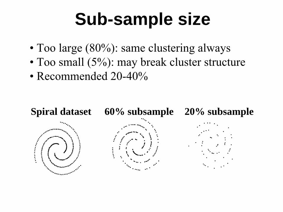
Sub-sample size

Spiral dataset 60% subsample 20% subsample

• Too large (80%): same clustering always• Too small (5%): may break cluster structure• Recommended 20-40%

Classification approach

Subsampling

Data set

Training subset Test subset

Clustering

Training

Clustering

Classifier ClusterValidity

Validity value[0, 1]

Model

Labels Labels

Labels

Does not really add anything more. Just makes process more complex.

Comparison of three approaches• Cross-validation works ok• Classification also ok• Randomizing algorithm fails

unstable

Too many clustersdifferent density

Too many clustersdifferent size

Too few clustersdifferent size

unstable

k=2 k=3 k=3

stable

Too many clusterswrong model

k=3

stable

ProblemStability can also come from other reasons:•

Different cluster sizes

•

Wrong cluster model Happens when k<k*

SolutionInstead of selecting k with maximum stability, select last

k with stable result.

Threshold=0.9

Effect of cluster shapes

Wrong model:•

Elliptical cluster Minimizing TSE would find 5 spherical clusters

Correct model:•

Works ok.

Which external index?Does not matter much•

This is not: RI

•

These all ok: ARI, NMI, PSI, NVD, CSI•

CI cares only allocation: sometimes too rough.

Does algorithm matter?Yes it does.•

Ok: Random Swap (RS) and Genetic Algorithm (GA)

•

Not: K-means (KM)

Summary•

The choice of the cross-validation strategy not critical

•

Last stable clustering instead of global maximum•

The choice of external index is not critical

•

Good clustering algorithm required (RS or GA)

Part V:

Efficient implementation

Strategies for efficient search

•

Brute force: solve clustering for all possible number of clusters.

•

Stepwise: as in brute force but start using previous solution and iterate less.

•

Criterion-guided search: Integrate cost function directly into the optimization function.

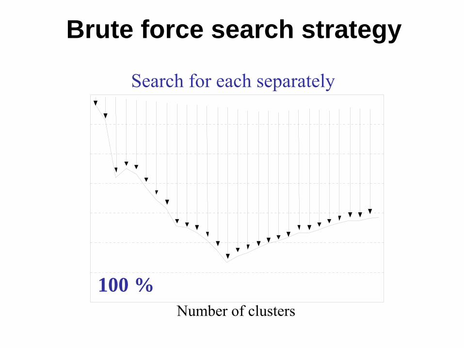
Brute force search strategy

Number of clusters

Search for each separately

100 %

Stepwise search strategy

Number of clusters

Start from the previous result

30-40 %

Criterion guided search

Number of clusters

Integrate with the cost function!

3-6 %

1 k/2 k 3k/2

f1

fk/2

fk

f3k/2

Eval

uatio

n fu

nctio

n va

lue

Iteration number

Starting point

Halfway

Current

Estimated

k

k

fffLTk

1

2/3min

Stopping criterion for stepwise search strategy

Comparison of search strategies

0102030405060708090

100

2 3 4 5 6 7 8 9 10 11 12 13 14 15

Data dimensionality

%

DLSCAStepwise/FCMStepwise/LBG-UStepwise/K-means

Open questions

Iterative algorithm (K-means or Random Swap) with criterion-guided

search … or …

Hierarchical algorithm ???Potential topic for

MSc or PhD thesis !!!

Part VI:

External indexes

The number of pairs that are in:

Same class both in P and G.

Same class in P but different in G.

Different classes in P but same in G.

Different classes both in P and G.

Pair-counting measures

G P

a

b

c

d

ab

cd

)(21 '

1 1

'

1

22

K

j

K

i

K

jijj nmb

)(21

1 1

'

1

22

K

i

K

i

K

jiji nnc

))((21 '

1

2

1

2

1

'

1

22

K

jj

K

ii

K

i

K

jij mnnNd

K

i

K

jijij nna

1

'

1

)1(21

dcbadaGPRI

),(

Rand index [Rand, 1971]

Rand index

= (20+72) / (20+24+20+72) = 92/136 = 0.68

G P

a

b

c

d

a

b

cd

a = 20

b = 24d = 72

c = 20

Rand and Adjusted Rand index [Hubert and Arabie, 1985]

)(1)(

RIERIERIARI

Adjusted Rand = (to be calculated) = 0.xx

G P

a

b

c

d

a

b

cd

a = 20

b = 24d = 72

c = 20

Rand statistics Positive examples

G P G P

a = 20 d = 72

Rand statistics Negative examples

G P G P

b = 24 c = 20

•

Pair counting•

Information theoretic

•

Set matching

External indexes

-

Based on the concept of entropy-

Mutual Information (MI): the shared informatio:

-

Variation of Information (VI) is complement of MI

Information-theoretic measures

K

i

K

j ji

jiji GpPp

GPpGPpGPMI

1

'

1 )()(),(

log),(),(

MI

H(G) H(P)

VI

H(P|G) H(G|P)

Categories–

Point-level

–

Cluster-level

Three problems–

How to measure the similarity of two clusters?

–

How to pair clusters?–

How to calculate overall similarity?

Set-matching measures

Measure: P1

, P2 P1

, P3

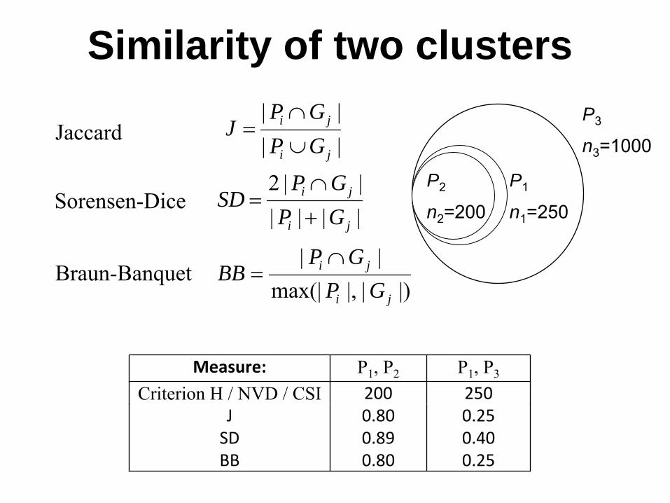
Criterion H / NVD / CSI 200 250J 0.80 0.25SD 0.89 0.40BB 0.80 0.25

||||

ji

ji

GPGP

J

||||||2

ji

ji

GPGP

SD

Jaccard

Sorensen-Dice

|)||,max(|||

ji

ji

GPGP

BB

P3

n3

=1000

P1

n1

=250

P2

n2

=200

Braun-Banquet

Similarity of two clusters

Every cluster is mapped to the cluster with maximum overlap

Matching

G P

G1 G2

G3

P1

P3

P2

Optimal pairing by Hungarian algorithm or greedy pairing

Pairing

G

P

4 1610 10

20 15 25

G P

G1G2

G3

P1

P2

P3

G P

G1G2

G3

P1

P2

P3

Matching vs. Pairing

Pairing/

Matching Matching criterion

Algorithm

FM Matching SD One-way CH Pairing |Pi ∩ Gj| Greedy

NVD Matching |Pi ∩ Gj| Two-way Purity Matching |Pi ∩ Gj| One-way

PSI Pairing BB Optimal CI Matching Centroid distance Two-way

CSI Matching Centroid distance Two-way CR Pairing Centroid distance Greedy

Summary of matching

Total summation Range Normalization

FM similarity of matched clusters [0, 1] N

CH Shared objects [0, 1] N

NVD Shared objects in both directions [0, 1] 2N

Purity Shared objects in one direction [0, 1] N

PSI Normalized

similarity of paired clusters

[0, 1] K

CI Orphan clusters [0, K-1] -

CSI Shared objects in both directions [0, 1] 2N

CR Unstable clusters [0, 1] K

Overall similarity

Closely related to Purity and CSI(Assumed that matching is symmetric)

Normalized Van Dongen

CSIPurityCHN

n

N

n

N

nnNVD

K

iij

K

iij

K

jji

K

iij

111

2

21

21

1

111

–

Similarity of two clusters:

–

Total similarity:

–

Pairing by Hungarian:

|)||,max(| ji

ijij GP

nS

1ijS

1jiS

5.0ijS

5.0jiS

S=100%

S=50%

Gj Pi

i

ijPG SS

Pair Set Index (PSI)M. Rezaei

and P. Fränti, "Set matching measures for external cluster validity", IEEE Trans. on Knowledge and Data Engineering, August 2016.

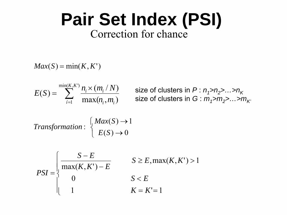
Correction for chance

)',min()( KKSMax

)',min(

1 ),max()/()(

KK

í ii

ii

mnNmnSE size of clusters in P : n1 >n2 >…>nK

size of clusters in G : m1 >m2 >…>mK’

0)(1)(

:SE

SMaxtionTransforma

Pair Set Index (PSI)

1'10

1)',max(,)',max(

KKES

KKESEKK

ES

PSI

•

Symmetric•

Normalized to number of clusters

•

Normalized to size of clusters•

Adjusted

•

Range in [0,1]•

Number of clusters can be different

Properties of PSI

Random partitioningChanging number of clusters in P from 1 to 20

1000 2000 3000 G

P

MonotonicityEnlarging the first cluster

1000 2000 3000G

1250 2000 3000 P1

2000 3000 P2

2500 3000 P3

3000 P4

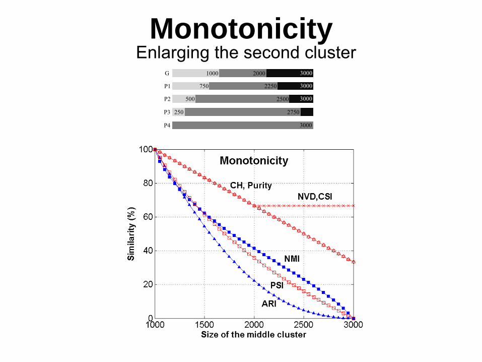
MonotonicityEnlarging the second cluster

1000 2000 3000 G

750 2250 3000 P1

500 2500 3000 P2

250 2750 P3

3000 P4

Cluster size imbalanceSame error in first two clusters

800 1800 3000 P1

1000 2000 3000 G1

800 1800 2500 P2

1000 2000 2500 G2

Number of clustersAlways 200 errors; k varies

800 1800 2800 P2

1000 2000 3000 G2

800 1800 P1

1000 2000 G1

Overlap and dimensionalityTwo clusters with varying overlap and dimensions

Overlap varies Dimensions

492

490 560458 1011

989

2000

500

K-means

Single link

2000

2000 2000

100

100

99

200

1

External indexes Algorithms

ARI NMI NVD PSI

RS 1.00 1.00 1.00 1.00

AC 1.00 1.00 1.00 1.00

SL 1.00 0.99 0.99 0.78

KM 0.66 0.77 0.78 0.18

Unbalance

Unrealistic high

Part VII:

Cluster-level measure

Comparing partitions of centroids

Point-level differences Cluster-level mismatches

Centroid index (CI)[Fränti, Rezaei, Zhao, Pattern Recognition, 2014]

Given two sets of centroids C and C’, find nearest neighbor mappings (CC’):

Detect prototypes with no mapping:

Centroid index:

1,1 ,'minarg2

21Kiccq ji

Kji

otherwise 0,

,1' ijqcorphan i

j

2

'1

1, '

K

jj

CI C C orphan c

Number of zero mappings!

11

11

2211

11

11

11

00

11

22

11

11

1111

00

Data Data SS22

Example of centroid index

Value 1 indicate same clusterIndex-value equals to the

count of zero-mappings

Mappings

Counts

CI = 2

Example of the Centroid index

Two clusters but only one

allocated

Three mapped into one

11

11

00

11

33

11

K-meansRandom Swap

Merge-based (PNN)

ARI=0.88CI=1

ARI=0.82CI=1

ARI=0.91CI=0

Adjusted Rand vs. Centroid index

•

Mapping is not symmetric (CC’

≠

C’C)•

Symmetric centroid index:

•

Pointwise

variant (Centroid Similarity Index):–

Matching clusters based on CI

–

Similarity of clusters

CCCICCCICCCI ,',',max', 112

where2

2112 SSCSI

N

CCS

K

iji

1

112 N

CCS

K

jij

2

121

Centroid index properties

1

2 43 0 0.87

0 0.87

1 0.65

10.56

10.56

10.53

Distance to ground truth (2 clusters):1 GT CI=1 CSI=0.502 GT CI=1 CSI=0.503 GT CI=1 CSI=0.504 GT CI=1 CSI=0.50

Centroid index

Data setClustering quality (MSE)

KM RKM KM++ XM AC RS GKM GABridge 179.76 176.92 173.64 179.73 168.92 164.64 164.78 161.47House 6.67 6.43 6.28 6.20 6.27 5.96 5.91 5.87

Miss America 5.95 5.83 5.52 5.92 5.36 5.28 5.21 5.10House 3.61 3.28 2.50 3.57 2.62 2.83 - 2.44

Birch1 5.47 5.01 4.88 5.12 4.73 4.64 - 4.64Birch2 7.47 5.65 3.07 6.29 2.28 2.28 - 2.28Birch3 2.51 2.07 1.92 2.07 1.96 1.86 - 1.86

S1 19.71 8.92 8.92 8.92 8.93 8.92 8.92 8.92

S2 20.58 13.28 13.28 15.87 13.44 13.28 13.28 13.28

S3 19.57 16.89 16.89 16.89 17.70 16.89 16.89 16.89

S4 17.73 15.70 15.70 15.71 17.52 15.70 15.71 15.70

Mean Squared Errors

Data setAdjusted Rand Index (ARI)

KM RKM KM++ XM AC RS GKM GABridge 0.38 0.40 0.39 0.37 0.43 0.52 0.50 1House 0.40 0.40 0.44 0.47 0.43 0.53 0.53 1

Miss America 0.19 0.19 0.18 0.20 0.20 0.20 0.23 1House 0.46 0.49 0.52 0.46 0.49 0.49 - 1

Birch 1 0.85 0.93 0.98 0.91 0.96 1.00 - 1Birch 2 0.81 0.86 0.95 0.86 1 1 - 1Birch 3 0.74 0.82 0.87 0.82 0.86 0.91 - 1

S1 0.83 1.00 1.00 1.00 1.00 1.00 1.00 1.00S2 0.80 0.99 0.99 0.89 0.98 0.99 0.99 0.99S3 0.86 0.96 0.96 0.96 0.92 0.96 0.96 0.96S4 0.82 0.93 0.93 0.94 0.77 0.93 0.93 0.93

Adjusted Rand Index

Data setNormalized Mutual Information (NMI)


Miss America 0.64 0.64 0.63 0.64 0.64 0.66 0.66 1.00House 0.81 0.81 0.82 0.81 0.81 0.82 - 1.00Birch 1 0.95 0.97 0.99 0.96 0.98 1.00 - 1.00Birch 2 0.96 0.97 0.99 0.97 1.00 1.00 - 1.00Birch 3 0.90 0.94 0.94 0.93 0.93 0.96 - 1.00

S1 0.93 1.00 1.00 1.00 1.00 1.00 1.00 1.00S2 0.90 0.99 0.99 0.95 0.99 0.93 0.99 0.99S3 0.92 0.97 0.97 0.97 0.94 0.97 0.97 0.97S4 0.88 0.94 0.94 0.95 0.85 0.94 0.94 0.94

Normalized Mutual information

Data setNormalized Van Dongen (NVD)


Miss America 0.60 0.60 0.61 0.59 0.57 0.55 0.53 0.00House 0.40 0.37 0.34 0.39 0.39 0.34 - 0.00Birch 1 0.09 0.04 0.01 0.06 0.02 0.00 - 0.00Birch 2 0.12 0.08 0.03 0.09 0.00 0.00 - 0.00Birch 3 0.19 0.12 0.10 0.13 0.13 0.06 - 0.00

S1 0.09 0.00 0.00 0.00 0.00 0.00 0.00 0.00S2 0.11 0.00 0.00 0.06 0.01 0.04 0.00 0.00S3 0.08 0.02 0.02 0.02 0.05 0.00 0.00 0.02S4 0.11 0.04 0.04 0.03 0.13 0.04 0.04 0.04

Normalized Van Dongen

Data setC-Index (CI2 )

KM RKM KM++ XM AC RS GKM GA

Bridge 74 63 58 81 33 33 35 0House 56 45 40 37 31 22 20 0

Miss America 88 91 67 88 38 43 36 0House 43 39 22 47 26 23 --- 0Birch 1 7 3 1 4 0 0 --- 0Birch 2 18 11 4 12 0 0 --- 0Birch 3 23 11 7 10 7 2 --- 0

S1 2 0 0 0 0 0 0 0S2 2 0 0 1 0 0 0 0S3 1 0 0 0 0 0 0 0S4 1 0 0 0 1 0 0 0

Centroid Index

Data setCentroid Similarity Index (CSI)

KM RKM KM++ XM AC RS GKM GA

Bridge 0.47 0.51 0.49 0.45 0.57 0.62 0.63 1.00House 0.49 0.50 0.54 0.57 0.55 0.63 0.66 1.00

Miss America 0.32 0.32 0.32 0.33 0.38 0.40 0.42 1.00House 0.54 0.57 0.63 0.54 0.57 0.62 --- 1.00Birch 1 0.87 0.94 0.98 0.93 0.99 1.00 --- 1.00Birch 2 0.76 0.84 0.94 0.83 1.00 1.00 --- 1.00Birch 3 0.71 0.82 0.87 0.81 0.86 0.93 --- 1.00

S1 0.83 1.00 1.00 1.00 1.00 1.00 1.00 1.00S2 0.82 1.00 1.00 0.91 1.00 1.00 1.00 1.00S3 0.89 0.99 0.99 0.99 0.98 0.99 0.99 0.99S4 0.87 0.98 0.98 0.99 0.85 0.98 0.98 0.98

Centroid Similarity Index

Method MSEGKM Global K-means 164.78RS Random swap (5k) 164.64GA Genetic algorithm 161.47RS8M Random swap (8M) 161.02GAIS-2002 GAIS 160.72+ RS1M GAIS + RS (1M) 160.49+ RS8M GAIS + RS (8M) 160.43GAIS-2012 GAIS 160.68+ RS1M GAIS + RS (1M) 160.45+ RS8M GAIS + RS (8M) 160.39+ PRS GAIS + PRS 160.33+ RS8M

+ GAIS + RS (8M) + 160.28

High quality clustering

Main algorithm:+ Tuning 1+ Tuning 2

RS8M GAIS 2002 GAIS 2012

××

××

RS1M×

RS8M×

××

RS1M×

RS8M× ×

RS8M

RS8M --- 19 19 19 23 24 24 23 22GAIS (2002) 23 --- 0 0 14 15 15 14 16

+ RS1M 23 0 --- 0 14 15 15 14 13+ RS8M 23 0 0 --- 14 15 15 14 13

GAIS (2012) 25 17 18 18 --- 1 1 1 1+ RS1M 25 17 18 18 1 --- 0 0 1+ RS8M 25 17 18 18 1 0 --- 0 1+ PRS 25 17 18 18 1 0 0 --- 1

+ RS8M

+ PRS 24 17 18 18 1 1 1 1 ---

Centroid index values

Summary of external indexes (existing measures)

Literature

1.

G.W. Milligan, and M.C. Cooper, “An examination of procedures for determining the number of clusters in a data set”, Psychometrika, Vol.50, 1985, pp. 159-179.

2.

E. Dimitriadou, S. Dolnicar, and A. Weingassel, “An examination of indexes for determining the number of clusters in binary data sets”, Psychometrika, Vol.67, No.1, 2002, pp. 137-160.

3.

D.L. Davies and D.W. Bouldin, "A cluster separation measure “,

IEEE Transactions on Pattern Analysis and Machine Intelligence, 1(2), 224-

227, 1979.4.

J.C. Bezdek

and N.R. Pal, "Some new indexes of cluster validity “,

IEEE

Transactions on Systems, Man and Cybernetics, 28(3), 302-315, 1998.5.

H. Bischof, A. Leonardis, and A. Selb, "MDL Principle for robust vector quantization“,

Pattern Analysis and Applications, 2(1), 59-72, 1999.

6.

P.

Fränti, M.

Xu

and I.

Kärkkäinen, "Classification of binary vectors by using DeltaSC-distance to minimize stochastic complexity", Pattern Recognition Letters, 24 (1-3), 65-73, January 2003.

7.

G.M. James, C.A. Sugar, "Finding the Number of Clusters in a Dataset: An Information-Theoretic Approach". Journal of the American Statistical Association, vol. 98, 397-408, 2003.

8.

P.K. Ito, Robustness of ANOVA and MANOVA Test Procedures. In: Krishnaiah

P. R. (ed), Handbook of Statistics 1: Analysis of Variance.

North-Holland Publishing Company, 1980.9.

I.

Kärkkäinen and P.

Fränti, "Dynamic local search for clustering with

unknown number of clusters", Int. Conf. on Pattern Recognition (ICPR’02), Québec, Canada, vol.

2, 240-243, August 2002.

10.

D. Pellag

and A. Moore, "X-means: Extending K-Means with Efficient Estimation of the Number of Clusters", Int. Conf. on Machine Learning (ICML), 727-734, San Francisco, 2000.

11.

S. Salvador and P. Chan, "Determining the Number of Clusters/Segments in Hierarchical Clustering/Segmentation Algorithms", IEEE Int. Con. Tools with Artificial Intelligence (ICTAI), 576-584, Boca Raton, Florida, November, 2004.

12.

M. Gyllenberg, T. Koski

and M. Verlaan, "Classification of binary vectors by stochastic complexity ". Journal of Multivariate Analysis, 63(1), 47-72, 1997.

Literature

Literature13.

M. Gyllenberg, T. Koski

and M. Verlaan, "Classification of binary vectors

by stochastic complexity ". Journal of Multivariate Analysis, 63(1), 47-72, 1997.

14.

X. Hu

and L. Xu, "A Comparative Study of Several Cluster Number Selection Criteria", Int. Conf. Intelligent Data Engineering and Automated Learning (IDEAL), 195-202, Hong Kong, 2003.

15.

Kaufman, L. and P. Rousseeuw, 1990. Finding

Groups in Data: An Introduction to Cluster Analysis. John Wiley and Sons, London. ISBN: 10:0471878766.

16.

[1.3] M.Halkidi, Y.Batistakis

and M.Vazirgiannis: Cluster validity methods: part 1, SIGMOD Rec., Vol.31, No.2, pp.40-45, 2002

17.

R. Tibshirani, G. Walther, T. Hastie. Estimating the number of clusters in a data set via the gap statistic. J.R.Statist. Soc. B(2001) 63, Part 2, pp.411-423.

18.

T. Lange, V. Roth, M, Braun and J. M. Buhmann. Stability-based validation of clustering solutions. Neural Computation. Vol. 16, pp. 1299-

1323. 2004.

Literature19.

Q.

Zhao, M.

Xu

and P.

Fränti, "Sum-of-squares based clustering validity

index and significance analysis", Int. Conf. on Adaptive and Natural Computing Algorithms (ICANNGA’09), Kuopio, Finland, LNCS 5495, 313-

322, April 2009. 20.

Q.

Zhao, M.

Xu

and P.

Fränti, "Knee point detection on bayesian

information

criterion", IEEE Int. Conf. Tools with Artificial Intelligence (ICTAI), Dayton, Ohio, USA, 431-438, November 2008.

21.

W.M. Rand, “Objective criteria for the evaluation of clustering methods,” Journal of the American Statistical Association, 66, 846–850, 1971

22.

L. Hubert and P. Arabie, “Comparing partitions”, Journal of Classification, 2(1), 193-218, 1985.

23.

P. Fränti, M. Rezaei and Q. Zhao, "Centroid index: cluster level similarity measure", Pattern Recognition, 47 (9), 3034-3045, September 2014, 2014.

24.

M. Rezaei and P. Fränti, "Set matching measures for external cluster validity", IEEE Trans. on Knowledge and Data Engineering, 28 (8), 2173-

2186, August 2016.25.

M.

Rezaei

and P.

Fränti

"Can the number of clusters be solved by external

index?", (submitted)

machine learning university of eastern finland -...

Documents