Original Manuscript

Title:

Machine vision detection to daily facial fatigue with a nonlocal 3D

attention network

Authors:

Zeyu Chen,1,2 Xinhang Zhang,1,2 Juan Li1,2, Jingxuan Ni1,3, Gang Chen4, Shaohua Wang4,

Fangfang Fan5, Changfeng Charles Wang6*, Xiaotao Li,1,2,7,8 # *

1. BIAI Intelligence Biotech Co., Ltd, Shenzhen 518055, GD, China; 2. BIAI Inc., Chelmsford,

MA 01824, USA. 3. Department of Mathematics, School of Science, Shantou University,

Shantou, GD, China. 4. Shenzhen Breo Technology CO., LTD., Shenzhen, GD, China. 5.

Department of Neurology, Harvard Medical School, Harvard University, Boston MA, USA. 6.

Stealth Mode Startup, INC., Chicago, Illinois, USA. 7. Shenzhen Key Lab of Neuropsychiatric

Modulation, Guangdong Provincial Key Laboratory of Brain Connectome and Behavior, CAS

Key Laboratory of Brain Connectome and Manipulation, CAS Center for Excellence in Brain

Science and Intelligence Technology, the Brain Cognition and Brain Disease Institute,

Shenzhen Institutes of Advanced Technology, Chinese Academy of Sciences; Shenzhen-Hong

Kong Institute of Brain Science-Shenzhen Fundamental Research Institutions, Shenzhen,

518055, China. 8. Department of Brain and Cognitive Sciences, Massachusetts Institute of

Technology, Cambridge, MA, USA.

*Corresponding author e-mail: xtli@mit.edu (X. Li)

Abstract:

Fatigue detection is valued for people to keep mental health and prevent safety accidents.

However, detecting facial fatigue, especially mild fatigue in the real world via machine vision

is still a challenging issue due to lack of non-lab dataset and well-defined algorithms. In order

to improve the detection capability on facial fatigue that can be used widely in daily life, this

paper provided an audiovisual dataset named DLFD (daily-life fatigue dataset) which reflected

people’s facial fatigue state in the wild. A framework using 3D-ResNet along with non-local

attention mechanism was training for extraction of local and long-range features in spatial and

temporal dimensions. Then, a compacted loss function combining mean squared error and

cross-entropy was designed to predict both continuous and categorical fatigue degrees. Our

proposed framework has reached an average accuracy of 90.8% on validation set and 72.5%

on test set for binary classification, standing a good position compared to other state-of-the-art

methods. The analysis of feature map visualization revealed that our framework captured facial

dynamics and attempted to build a connection with fatigue state. Our experimental results in

multiple metrics proved that our framework captured some typical, micro and dynamic facial

features along spatiotemporal dimensions, contributing to the mild fatigue detection in the wild.

Keywords: fatigue detection, in the wild, DLFD dataset, non-local attention, 3D-ResNet

1 Introduction

Fatigue is one of psychophysiological conditions with a feeling of physical or mental tiredness,

usually caused by exertion and then characterized by a decreased capacity for physical activity

and mental processing [1]. It can be roughly categorized to physical and mental parts, however,

physical fatigue mainly involves the over-taxation of the muscular system while mental fatigue

is a transient decrease in cognitive performance mainly induced by excessive demands on

cognitive systems [2]. Mental fatigue, also known as cognitive fatigue, often leads to a lowered

productivity and an increased risk of safety [3]; and long term of mental fatigue (2-3 weeks)

can even be as one of major symptoms for major depression [4]. Hence, in-time detection of

mental fatigue will largely contribute to the balance of work arrange and life satisfaction and

even prevent fatigue-related brain disorders.

In terms of facial fatigue detection, people can perceive their own fatigue and the fatigue can

be also observed by others through some typical features on their faces such as droopy eyes,

long blinks and yawning [5]. PERCLOS (percentage of eyelid closure over the pupil over time)

[6] and eye aspect ratio [7] are both widely used as metrics to judge drowsiness level via

measuring the degree of eye closure and the frequency of eye blink. And statistical analysis can

be applied based on these drowsiness-related indicators to measure individuals’ fatigue level,

which have been widely applied in some situations like driving monitor system (DMS) [8].

However, those traditionally statistical methods including haar-like feature [9] and Adaboost

classifier [10] are limited to detect a severe state of fatigue. In terms of detection for mild and

modern fatigue, deep learning algorithms especially convolutional neural networks (CNN)

have already showed some advantages over traditional ones [11]. To develop a better detection

for facial fatigue in daily life, two major trends with computer vision have showed in the current

facial fatigue detection: one is a transition from image-based detection [12-16] to video-based

detection [17-22], and the other is from experimentally simulated data to the data collected in

the real-world scenario. Though the existing methods have achieved up to 97% accuracy [18],

most of them used well-known fatigue datasets like NTHU-DDD [23] and YawDD [24], which

were either simulated in the laboratory or collected at vehicle-mimicking conditions [25].

Those methods were sufficiently effective when there were distinct features between fatigue

and alert state. However, in many situations in real life the fatigue is not obvious so that facial

fatigue detection especially for mild fatigue is still a challenge in the wild.

In order to improve fatigue detection level that it can be widely used in different life scenarios

in the wild, we proposed an audiovisual dataset named DLFD (daily-life fatigue dataset),

containing people’s natural facial status at different conditions. Furthermore, we employed

paradigms of 3D CNN and non-local attention blocks to increase the ability of our models in

recognizing mild fatigue in the wild. Through the experiments on dataset of DLFD, we proved

the effectiveness and advantages of our model.

2 Materials and Methods

2.1 Dataset Properties and Description

DLFD dataset consists of 375 videos with about 20,000 frames length of which varies from 5

seconds to 2 minutes. The mean resolution for these videos is approximately 1056 x 629 and

mean frame rate is 30 fps. The facial videos in the dataset are self-captured by 32 volunteers

when they are in different life scenarios such as awaking, working, off work, breaking, etc. and

at different time from morning to midnight. To some extent, this collection recorded people's

natural rather than faked fatigue state as much as possible, thus accurately reflected people’s

fatigue degree in the wild. DLFD dataset was labeled independently by three psychology-based

annotators based on subjectives’ self-evaluation. According to the visual and acoustic

information contained in volunteers’ video, annotators evaluated their degree of fatigue ranging

from 1 to 5. 1 represents very significant alert state and 5 represents very significant fatigue

state. We calculated two types of labels, one of which for continuous task and the other for

categorical task. The former one is calculated by the mean evaluation of three annotators and

the latter one is deduced from the mean evaluation by isometric binning techniques. For

simplicity, we call them continuous and categorical label respectively.

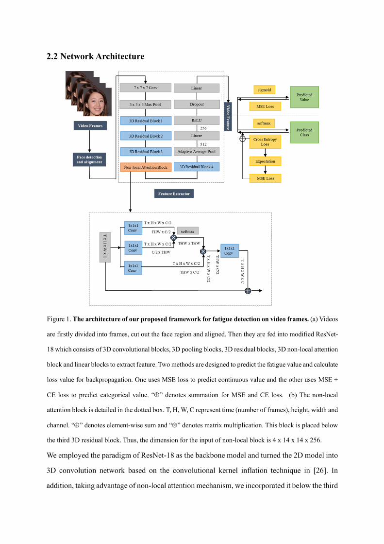
2.2 Network Architecture

We employed the paradigm of ResNet-18 as the backbone model and turned the 2D model into

3D convolution network based on the convolutional kernel inflation technique in [26]. In

addition, taking advantage of non-local attention mechanism, we incorporated it below the third

Figure 1. The architecture of our proposed framework for fatigue detection on video frames. (a) Videos

are firstly divided into frames, cut out the face region and aligned. Then they are fed into modified ResNet-

18 which consists of 3D convolutional blocks, 3D pooling blocks, 3D residual blocks, 3D non-local attention

block and linear blocks to extract feature. Two methods are designed to predict the fatigue value and calculate

loss value for backpropagation. One uses MSE loss to predict continuous value and the other uses MSE +

CE loss to predict categorical value. “” denotes summation for MSE and CE loss. (b) The non-local

attention block is detailed in the dotted box. T, H, W, C represent time (number of frames), height, width and

channel. “” denotes element-wise sum and “” denotes matrix multiplication. This block is placed below

the third 3D residual block. Thus, the dimension for the input of non-local block is 4 x 14 x 14 x 256.

basic block in 3D-ResNet. Noted that different from the single linear layer design in classic

ResNet, we appended two fully connected layers after convolution blocks. It is noteworthy that

one of our novel works here was the adoption of both mean squared error loss function and

cross entropy loss function in fatigue level prediction. This strategy was motivated by

construction of loss function in multi-task learning and realized by an expectation

transformation technique, which was illustrated below in the section of loss function. The

softmax layer was first used to categorize the features extracted by linear blocks and through

expectation transformation, the categorical prediction could be transformed to a continuous

value for the calculation of MSE loss. The overall network architecture is presented by Figure

1.

2.3 Non-local Attention Module

The non-local attention has been viewed as a way to take global information into consideration

in constructing feature map, showing its advantage in many applications of computer vison like

image restoration and people reidentification [27, 28]. According to the work of Wang et al.

[26], here we give a general introduction to non-local attention block. Following their work,

the non-local operation on convolutional networks can be defined by:

1

( , ) (( )

)j

j

i i jy f x x g xC x

= (2.4.1)

The equation above shows the calculation of output features iy given input features ix . Here i

represents the index of current response (i.e., feature) from either spatial or temporal dimension

and j represents the index of global response from all dimensions. Function f measures the

affinity between the i-th feature and the j-th feature, and function g projects the given

features x into a feature space. ( )C x is a normalization factor. In our work, we adopted the

embedded gaussian form mentioned in [26] in calculating f since it is a natural extension of

the self-attention blocks widely used in sequence models. Here is the architecture of our non-

local attention module:

The non-local attention module tackles long-term dependencies in spatial and temporal

dimensions from four major steps:

⚫ 1 x 1 convolution is adopted to respectively generate two feature spaces ( ), v( )u x x given

input feature x , which are defined as: ( () , v )u vx x W xu x W == . The autocorrelation of

features is calculated by dot product of feature spaces i.e., )( ()T vx xu . Here )( ()T

i jvx xu

represents the relationship between i-th feature and j-th feature.

⚫ Considering the embedded gaussian format of f in equation (2.4.1) and the need of

normalization, outputs in step 1 pass softmax to form attention map. The attention weight

from the i-th feature to the j-th feature is given by:

1

( ( ))

exp( ), )

exp(

ij T

ij ij i

j

j

ij

N

ss u vx x

s

=

= =

(2.4.2)

⚫ Based on the attention weight, original feature x is first projected to another feature space

through function g , and then summed up along j-th dimension to produce self-attention

feature map. Given activation function A, the self-attention feature iy is calculated by:

( ( ))ji ij jy A g x

= (2.4.3)

⚫ Motivated by the method in residual network, the self-attention feature and original feature

are synthesized to calculate the non-local output iz :

i z i iz y x= + (2.4.4)

Noted that z is trainable parameter which is initialized by zero. It indicates that in the

beginning of training, local information generated by the convolution is more heavily relied,

and gradually non-local information is introduced to grasp information of larger scope.

2.4 Loss Function

In order to gain continuous value for fatigue measurement, at the first stage of our research we

used mean square error as loss function and added a sigmoid layer in the end to achieve

predictions between 0 and 1. However, it should be pointed out that using only mean squared

error as loss function has some defects. Due to the mathematical property of the derivative

derived by combining sigmoid with MSE, optimization might be easy to fall into a local

minimum. Additionally, we also preferred to train a categorical model so that it could be

compared with other state-of-the-art models. During the design of this categorical model, since

both categorical and continuous predictions for evaluating fatigue degree were expected to

obtain through the network, we designed a loss function which combines MSE and cross

entropy loss together by the inspersion of multi-class learning. The motivation behind this idea

is instinct that the featured extracted by networks can be activated by sigmoid function and

evaluated by cross entropy loss to avoid gradient problems caused by the combination of

sigmoid and MSE. Also, since the information is more detailed when using continuous label,

the introduction of MSE loss helps the network better learn the matching rules between features

and labels, thereby reducing the difficulty of learning. The challenge in this part is the

continuous prediction for fatigue given the output of sigmoid layer. Here we borrowed the

method from the work of Ruiz et al. [29] and designed a strategy named expectation

transformation which transformed the probability of fatigue from sigmoid layer to a continuous

value between 0 and 1 representing fatigue prediction. Specifically, the fatigue value from 0 to

1 can be binned to two intervals, [0, 0.5) and [0.5, 1]. The probability that the fatigue value

falls within the corresponding interval is given by the sigmoid output and the midpoints of

these intervals can be viewed as their representation. In this way, mathematical expectation

defined in discreate random variable can be calculated and regarded as the continuous

prediction.

Noted that our proposed expectation transformation strategy was easily generalized to multi-

class task, so the usage of our model architecture is not limited to binary-class situation. Here

we derive the mathematical form of our expectation transformation in multi-class situation.

Supposed that we have k neurons in softmax layer which will predict probabilities for k

classes. Given sample j and class i , jiq is the predicted probability by softmax layer. The

fatigue value will be divided into different bins determined by k :1

[ , ), 1,..., 1i i

i kk k

+= − .

Using the midpoints of these bins, the continuous prediction of fatigue can be given by:

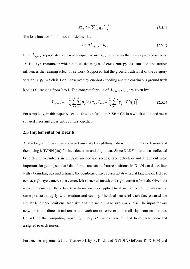
1

2 1( )

i j

k

ij

iE q q

k=

+= (2.5.1)

The loss function of our model is defined by:

softmax mseL L L= + (2.5.2)

Here softmaxL represents the cross-entropy loss and mseL represents the mean squared error loss.

is a hyperparameter which adjusts the weight of cross entropy loss function and further

influences the learning effect of network. Supposed that the ground truth label of the category

version is jip , which is 1 or 0 generated by one-hot encoding and the continuous ground truth

label is jy ranging from 0 to 1. The concrete formula of ,softmax mseL L are given by:

2

1 1 1

1 1log , ( )softmax ji ji ms

N k N

j

j

i j

e jL p q L y E qN N= = =

= − = − (2.5.3)

For simplicity, in this paper we called this loss function MSE + CE loss which combined mean

squared error and cross entropy loss together.

2.5 Implementation Details

At the beginning, we pre-processed our data by splitting videos into continuous frames and

then using MTCNN [30] for face detection and alignment. Since DLDF dataset was collected

by different volunteers in multiple in-the-wild scenes, face detection and alignment were

important for getting standard data format and stable feature positions. MTCNN can detect face

with a bounding box and estimate the positions of five representative facial landmarks: left eye

center, right eye center, nose center, left corner of mouth and right corner of mouth. Given the

above information, the affine transformation was applied to align the five landmarks to the

same position roughly with rotation and scaling. The final frame of each face ensured the

similar landmark positions, face size and the same image size 224 x 224. The input for our

network is a 4-dimensional tensor and each tensor represents a small clip from each video.

Considered the computing capability, every 32 frames were divided from each video and

assigned to each tensor.

Further, we implemented our framework by PyTorch and NVIDIA GeForce RTX 3070 and

GeForce RTX 2080Ti. We transferred a 2D ResNet-18 model pretrained on MS-Celeb-1M face

recognition dataset [31] to 3D model by inflating the kernels [32]. Specifically, each of the t

dimension of 3D kernel t x k x k are initialed by pre-trained k x k weights of the corresponding

2D kernels. For our framework with MSE loss, we used the total 375 samples in DLFD dataset,

and trained with a starting learning rate of 0.00001, weight decay of 0.1, batch size of 32 and

use Adam with default values as the optimizer. We used learning rate decay and given a certain

number of iterations, the learning rate was reduced by 0.2 times at 1/3 and 2/3 respectively.

Additionally, we resized the input image to 112 x 112 to make the computation complete on

one GPU. Thus, the size of the final input tensor was 32 x 3 x 112 x 112. For our framework

with MSE + CE loss which produced categorical prediction, we selected 69 samples and trained

with the same learning rate and decay method, weight decay of 0.001, batch size of 16, Adam

optimizer as well as the resized input image of 224 x 224. In this case, the size of the final input

tensor was 32 x 3 x 224 x 224 (Fig 1).

For the sake of improving the generalization ability of the model and avoiding obvious

overfitting, we adopted up to 6 kinds of data augmentations including random horizontal

flipping, gaussian blur as well as random changes on image lightness, contrast and saturation.

We composed these changes together and introduced a probability of 0.5 so that the occurrence

of each augmentation can be randomized. Noticed that above augmentations were fixed and

remained the same in one tensor, which was one 32-frame clip from a video, while randomized

and varied among different clips. Additionally, early stop was used and twenty epochs was set

as the patience.

3 Results

3.1 Comparison

During our experiments, we attempted to test multiple hyperparameter combinations and

different backbone models. In addition, we compared the effect of non-local attention block on

our model performances, with no attention block, attention block adding at different residual

blocks, respectively. Two kinds of loss functions were used for evaluation: one was MSE loss

and the other was MSE + CE loss. Unless otherwise specified, the following experiments all

used the total 375 samples in DLFD dataset, the pre-trained framework with non-local attention

mechanism placed below the third residual block, and default hyperparameter settings

illustrated in the section of 2.5, implementation details. Each comparison adopts the controlled

variable method to ensure that the hyperparameters and method settings related to model

training other than the variable to be compared remain unchanged.

3.1.1 The effect of batch size and data augmentation

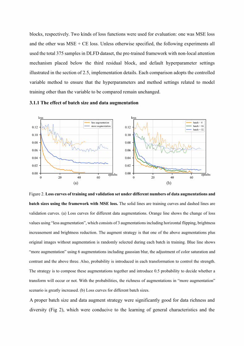
A proper batch size and data augment strategy were significantly good for data richness and

diversity (Fig 2), which were conducive to the learning of general characteristics and the

Figure 2. Loss curves of training and validation set under different numbers of data augmentations and

batch sizes using the framework with MSE loss. The solid lines are training curves and dashed lines are

validation curves. (a) Loss curves for different data augmentations. Orange line shows the change of loss

values using “less augmentation”, which consists of 3 augmentations including horizontal flipping, brightness

increasement and brightness reduction. The augment strategy is that one of the above augmentations plus

original images without augmentation is randomly selected during each batch in training. Blue line shows

“more augmentation” using 6 augmentations including gaussian blur, the adjustment of color saturation and

contrast and the above three. Also, probability is introduced in each transformation to control the strength.

The strategy is to compose these augmentations together and introduce 0.5 probability to decide whether a

transform will occur or not. With the probabilities, the richness of augmentations in “more augmentation”

scenario is greatly increased. (b) Loss curves for different batch sizes.

generalization of model. With the framework with MSE loss, we tried batch size of 4, 16 and

32 on 100 samples, and also two data augmentation strategies with the difference on

augmentation diversity (1st: 3 augmentations including horizontal flipping, brightness

increasement and brightness reduction, 2nd: 6 augmentations including the above three,

gaussian blur as well as the adjustment of color saturation and contrast). In each experiment,

we ensured the other control variables remained the same. Figure 2 showed that the training

and validation loss curve with the batch size of 32 were the smoothest and the number of epochs

before early stop is the most. In addition, compared with “less augmentation” strategy of 3

augmentations, “more augmentation” strategy of 6 augmentations shortened the discrepancy

of the loss between training and validation set, and prolonged iteration times before early stop

as well. Hence, in the following experiments below, we all used the batch size of 32 and “more

augmentation” strategy of 6 augmentations.

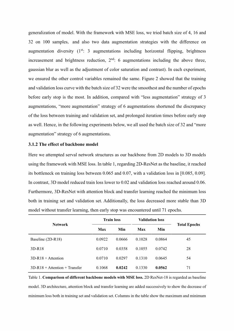
3.1.2 The effect of backbone model

Here we attempted serval network structures as our backbone from 2D models to 3D models

using the framework with MSE loss. In table 1, regarding 2D-ResNet as the baseline, it reached

its bottleneck on training loss between 0.065 and 0.07, with a validation loss in [0.085, 0.09].

In contrast, 3D model reduced train loss lower to 0.02 and validation loss reached around 0.06.

Furthermore, 3D-ResNet with attention block and transfer learning reached the minimum loss

both in training set and validation set. Additionally, the loss decreased more stable than 3D

model without transfer learning, then early stop was encountered until 71 epochs.

Network

Train loss Validation loss

Total Epochs

Max Min Max Min

Baseline (2D-R18) 0.0922 0.0666 0.1028 0.0864 45

3D-R18 0.0710 0.0358 0.1055 0.0742 28

3D-R18 + Attention 0.0710 0.0297 0.1310 0.0645 54

3D-R18 + Attention + Transfer 0.1068 0.0242 0.1330 0.0562 71

Table 1. Comparison of different backbone models with MSE loss. 2D ResNet-18 is regarded as baseline

model. 3D architecture, attention block and transfer learning are added successively to show the decrease of

minimum loss both in training set and validation set. Columns in the table show the maximum and minimum

loss of training and validation set. Additionally, the number of total epochs before early stop is added, which

shows that overfitting is not easy to trigger after adding attention block and transfer learning.

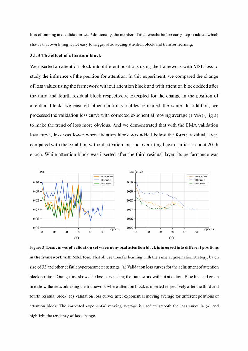
3.1.3 The effect of attention block

We inserted an attention block into different positions using the framework with MSE loss to

study the influence of the position for attention. In this experiment, we compared the change

of loss values using the framework without attention block and with attention block added after

the third and fourth residual block respectively. Excepted for the change in the position of

attention block, we ensured other control variables remained the same. In addition, we

processed the validation loss curve with corrected exponential moving average (EMA) (Fig 3)

to make the trend of loss more obvious. And we demonstrated that with the EMA validation

loss curve, loss was lower when attention block was added below the fourth residual layer,

compared with the condition without attention, but the overfitting began earlier at about 20-th

epoch. While attention block was inserted after the third residual layer, its performance was

Figure 3. Loss curves of validation set when non-local attention block is inserted into different positions

in the framework with MSE loss. That all use transfer learning with the same augmentation strategy, batch

size of 32 and other default hyperparameter settings. (a) Validation loss curves for the adjustment of attention

block position. Orange line shows the loss curve using the framework without attention. Blue line and green

line show the network using the framework where attention block is inserted respectively after the third and

fourth residual block. (b) Validation loss curves after exponential moving average for different positions of

attention block. The corrected exponential moving average is used to smooth the loss curve in (a) and

highlight the tendency of loss change.

further improved since a loss descended smoothly to a lower stage after serval epochs without

encountering overfitting, though initial loss was higher.

Attention Block Position

Train loss Validation loss

Total Epochs

Max Min Max Min

Without attention 0.1025 0.0259 0.0946 0.0589 40

After residual block 3 0.1117 0.0251 0.1011 0.0578 61

After residual block 4 0.1084 0.0329 0.0808 0.0614 33

Table 2. Comparison of loss values when non-local attention block is inserted into different positions

in the framework with MSE loss. That all use transfer learning with the same augmentation strategy, batch

size of 32 and other default hyperparameter settings. When attention block inserts after the third residual

block, the minimum training loss and validation loss both achieve the lowest.

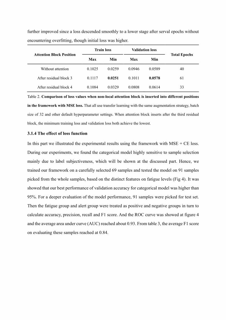
3.1.4 The effect of loss function

In this part we illustrated the experimental results using the framework with MSE + CE loss.

During our experiments, we found the categorical model highly sensitive to sample selection

mainly due to label subjectiveness, which will be shown at the discussed part. Hence, we

trained our framework on a carefully selected 69 samples and tested the model on 91 samples

picked from the whole samples, based on the distinct features on fatigue levels (Fig 4). It was

showed that our best performance of validation accuracy for categorical model was higher than

95%. For a deeper evaluation of the model performance, 91 samples were picked for test set.

Then the fatigue group and alert group were treated as positive and negative groups in turn to

calculate accuracy, precision, recall and F1 score. And the ROC curve was showed at figure 4

and the average area under curve (AUC) reached about 0.93. From table 3, the average F1 score

on evaluating these samples reached at 0.84.

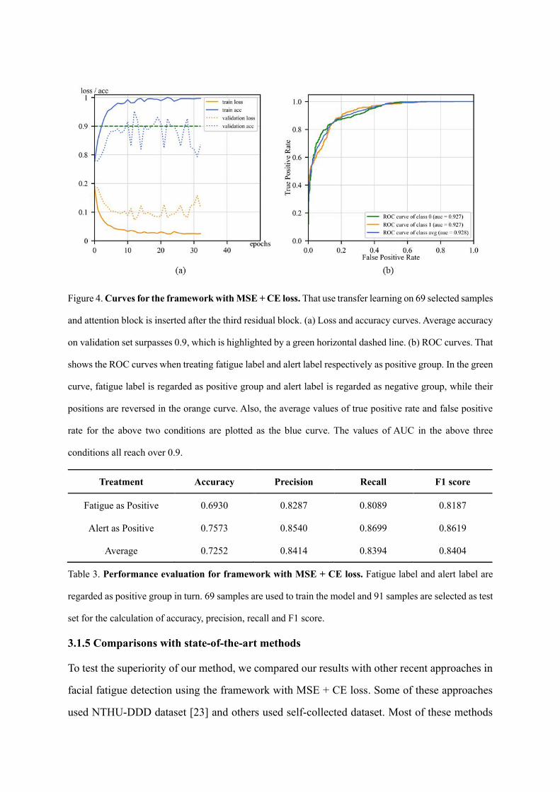
Figure 4. Curves for the framework with MSE + CE loss. That use transfer learning on 69 selected samples

and attention block is inserted after the third residual block. (a) Loss and accuracy curves. Average accuracy

on validation set surpasses 0.9, which is highlighted by a green horizontal dashed line. (b) ROC curves. That

shows the ROC curves when treating fatigue label and alert label respectively as positive group. In the green

curve, fatigue label is regarded as positive group and alert label is regarded as negative group, while their

positions are reversed in the orange curve. Also, the average values of true positive rate and false positive

rate for the above two conditions are plotted as the blue curve. The values of AUC in the above three

conditions all reach over 0.9.

Table 3. Performance evaluation for framework with MSE + CE loss. Fatigue label and alert label are

regarded as positive group in turn. 69 samples are used to train the model and 91 samples are selected as test

set for the calculation of accuracy, precision, recall and F1 score.

3.1.5 Comparisons with state-of-the-art methods

To test the superiority of our method, we compared our results with other recent approaches in

facial fatigue detection using the framework with MSE + CE loss. Some of these approaches

used NTHU-DDD dataset [23] and others used self-collected dataset. Most of these methods

Treatment Accuracy Precision Recall F1 score

Fatigue as Positive 0.6930 0.8287 0.8089 0.8187

Alert as Positive 0.7573 0.8540 0.8699 0.8619

Average 0.7252 0.8414 0.8394 0.8404

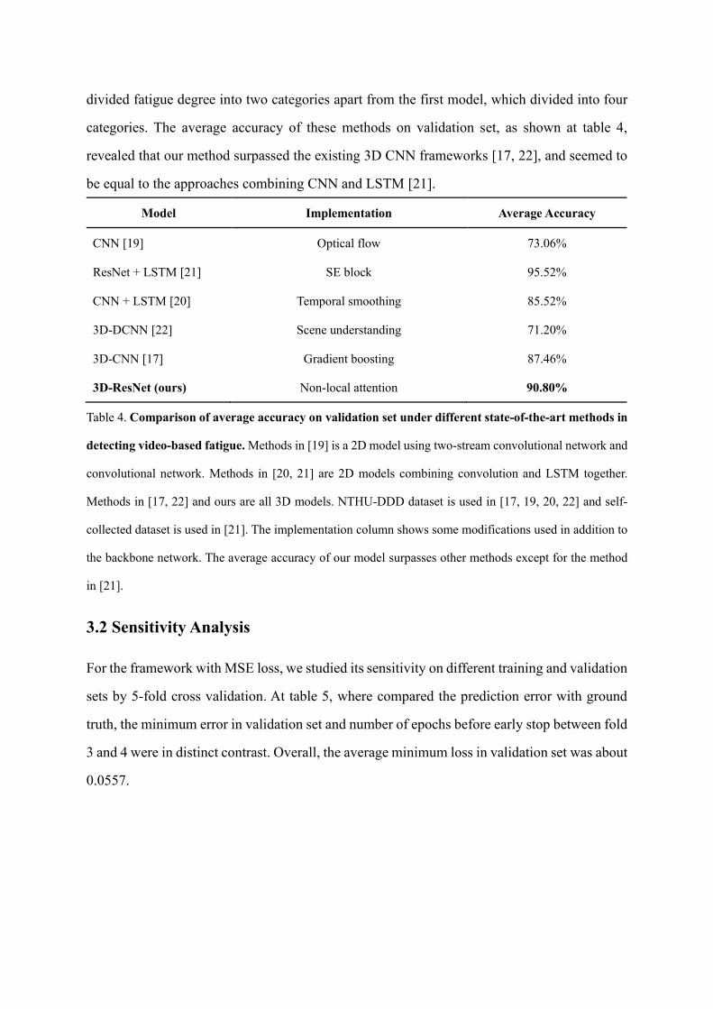
divided fatigue degree into two categories apart from the first model, which divided into four

categories. The average accuracy of these methods on validation set, as shown at table 4,

revealed that our method surpassed the existing 3D CNN frameworks [17, 22], and seemed to

be equal to the approaches combining CNN and LSTM [21].

Model Implementation Average Accuracy

CNN [19] Optical flow 73.06%

ResNet + LSTM [21] SE block 95.52%

CNN + LSTM [20] Temporal smoothing 85.52%

3D-DCNN [22] Scene understanding 71.20%

3D-CNN [17] Gradient boosting 87.46%

3D-ResNet (ours) Non-local attention 90.80%

Table 4. Comparison of average accuracy on validation set under different state-of-the-art methods in

detecting video-based fatigue. Methods in [19] is a 2D model using two-stream convolutional network and

convolutional network. Methods in [20, 21] are 2D models combining convolution and LSTM together.

Methods in [17, 22] and ours are all 3D models. NTHU-DDD dataset is used in [17, 19, 20, 22] and self-

collected dataset is used in [21]. The implementation column shows some modifications used in addition to

the backbone network. The average accuracy of our model surpasses other methods except for the method

in [21].

3.2 Sensitivity Analysis

For the framework with MSE loss, we studied its sensitivity on different training and validation

sets by 5-fold cross validation. At table 5, where compared the prediction error with ground

truth, the minimum error in validation set and number of epochs before early stop between fold

3 and 4 were in distinct contrast. Overall, the average minimum loss in validation set was about

0.0557.

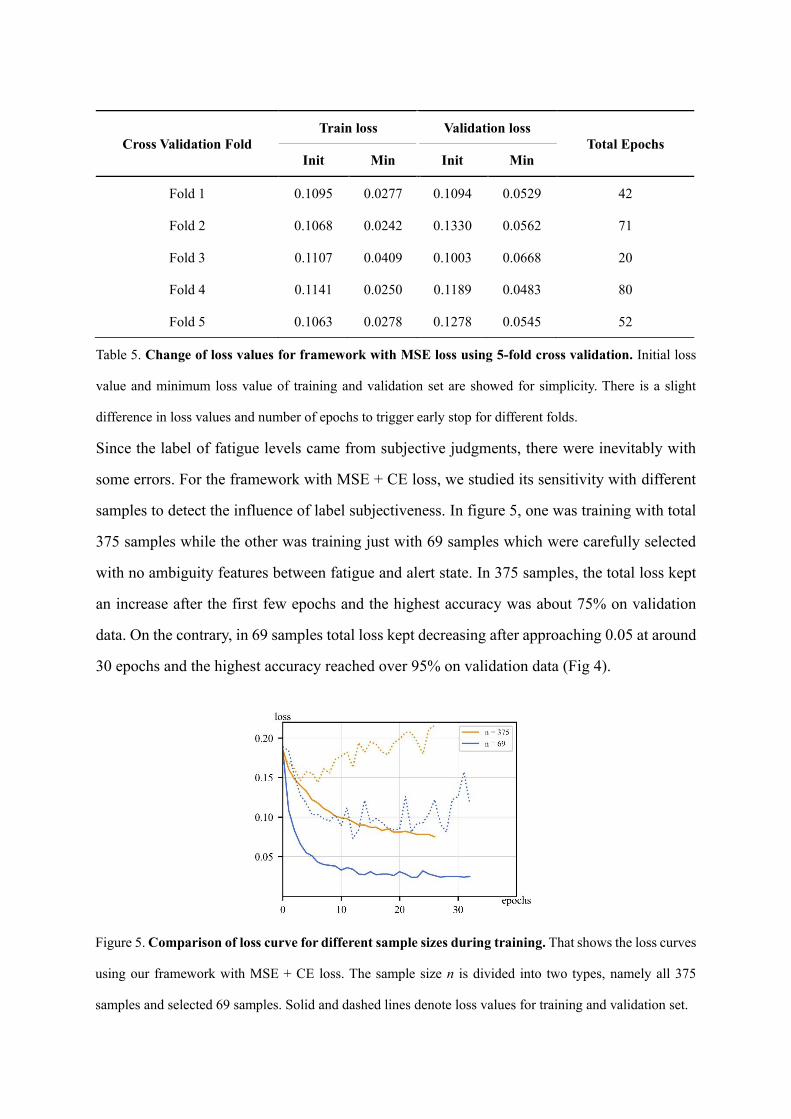
Table 5. Change of loss values for framework with MSE loss using 5-fold cross validation. Initial loss

value and minimum loss value of training and validation set are showed for simplicity. There is a slight

difference in loss values and number of epochs to trigger early stop for different folds.

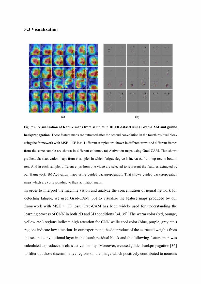
Since the label of fatigue levels came from subjective judgments, there were inevitably with

some errors. For the framework with MSE + CE loss, we studied its sensitivity with different

samples to detect the influence of label subjectiveness. In figure 5, one was training with total

375 samples while the other was training just with 69 samples which were carefully selected

with no ambiguity features between fatigue and alert state. In 375 samples, the total loss kept

an increase after the first few epochs and the highest accuracy was about 75% on validation

data. On the contrary, in 69 samples total loss kept decreasing after approaching 0.05 at around

30 epochs and the highest accuracy reached over 95% on validation data (Fig 4).

Cross Validation Fold

Train loss Validation loss

Total Epochs

Init Min Init Min

Fold 1 0.1095 0.0277 0.1094 0.0529 42

Fold 2 0.1068 0.0242 0.1330 0.0562 71

Fold 3 0.1107 0.0409 0.1003 0.0668 20

Fold 4 0.1141 0.0250 0.1189 0.0483 80

Fold 5 0.1063 0.0278 0.1278 0.0545 52

Figure 5. Comparison of loss curve for different sample sizes during training. That shows the loss curves

using our framework with MSE + CE loss. The sample size n is divided into two types, namely all 375

samples and selected 69 samples. Solid and dashed lines denote loss values for training and validation set.

3.3 Visualization

In order to interpret the machine vision and analyze the concentration of neural network for

detecting fatigue, we used Grad-CAM [33] to visualize the feature maps produced by our

framework with MSE + CE loss. Grad-CAM has been widely used for understanding the

learning process of CNN in both 2D and 3D conditions [34, 35]. The warm color (red, orange,

yellow etc.) regions indicate high attention for CNN while cool color (blue, purple, gray etc.)

regions indicate low attention. In our experiment, the dot product of the extracted weights from

the second convolutional layer in the fourth residual block and the following feature map was

calculated to produce the class activation map. Moreover, we used guided backpropagation [36]

to filter out those discriminative regions on the image which positively contributed to neurons

Figure 6. Visualization of feature maps from samples in DLFD dataset using Grad-CAM and guided

backpropagation. These feature maps are extracted after the second convolution in the fourth residual block

using the framework with MSE + CE loss. Different samples are shown in different rows and different frames

from the same sample are shown in different columns. (a) Activation maps using Grad-CAM. That shows

gradient class activation maps from 6 samples in which fatigue degree is increased from top row to bottom

row. And in each sample, different clips from one video are selected to represent the features extracted by

our framework. (b) Activation maps using guided backpropagation. That shows guided backpropagation

maps which are corresponding to their activation maps.

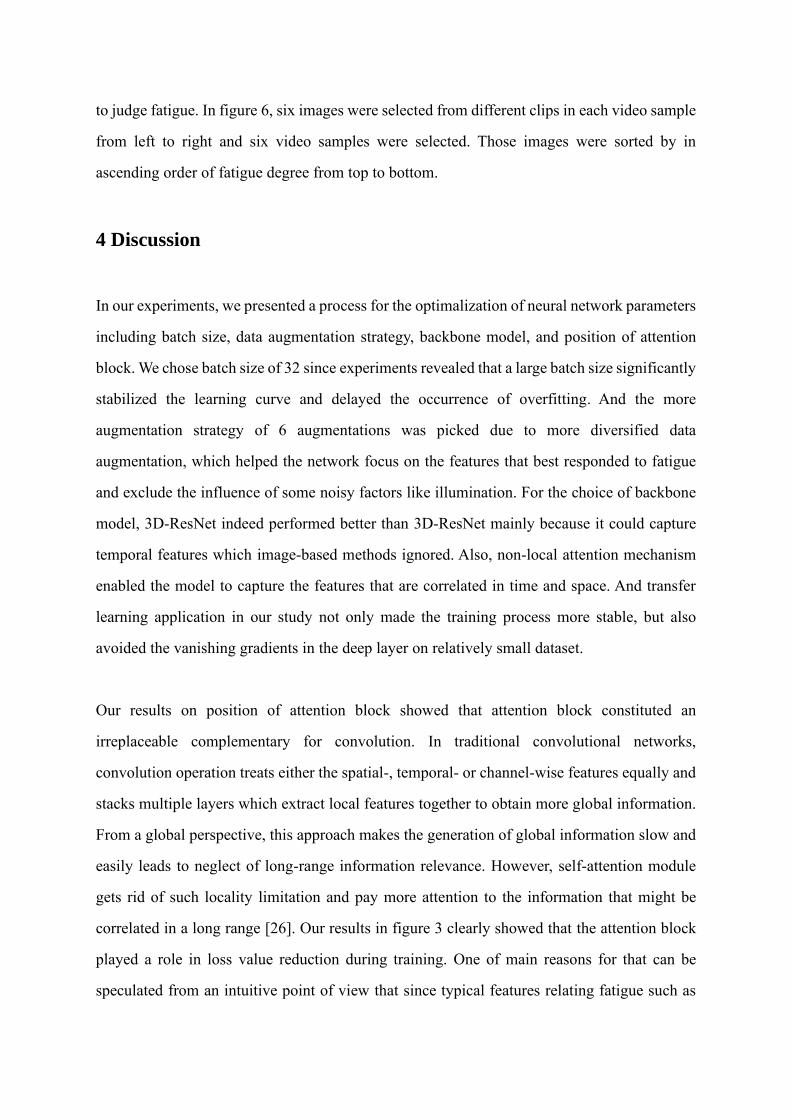
to judge fatigue. In figure 6, six images were selected from different clips in each video sample

from left to right and six video samples were selected. Those images were sorted by in

ascending order of fatigue degree from top to bottom.

4 Discussion

In our experiments, we presented a process for the optimalization of neural network parameters

including batch size, data augmentation strategy, backbone model, and position of attention

block. We chose batch size of 32 since experiments revealed that a large batch size significantly

stabilized the learning curve and delayed the occurrence of overfitting. And the more

augmentation strategy of 6 augmentations was picked due to more diversified data

augmentation, which helped the network focus on the features that best responded to fatigue

and exclude the influence of some noisy factors like illumination. For the choice of backbone

model, 3D-ResNet indeed performed better than 3D-ResNet mainly because it could capture

temporal features which image-based methods ignored. Also, non-local attention mechanism

enabled the model to capture the features that are correlated in time and space. And transfer

learning application in our study not only made the training process more stable, but also

avoided the vanishing gradients in the deep layer on relatively small dataset.

Our results on position of attention block showed that attention block constituted an

irreplaceable complementary for convolution. In traditional convolutional networks,

convolution operation treats either the spatial-, temporal- or channel-wise features equally and

stacks multiple layers which extract local features together to obtain more global information.

From a global perspective, this approach makes the generation of global information slow and

easily leads to neglect of long-range information relevance. However, self-attention module

gets rid of such locality limitation and pay more attention to the information that might be

correlated in a long range [26]. Our results in figure 3 clearly showed that the attention block

played a role in loss value reduction during training. One of main reasons for that can be

speculated from an intuitive point of view that since typical features relating fatigue such as

eye blinking and yawning are continuous actions which spanned multiple frames and mobilized

multiple facial muscles, the attention block can be useful for building the correlation of these

muscle movements across frames. However, the relationship between the position of attention

block and the degree of loss value reduction is not clear so far [26-28]. It often highly depends

on other settings of hyperparameter and network structures. From a practical and convenient

point of view, one non-local block inserting into one convolutional layer is sufficient for

accuracy improvement of our model.

Our results on loss functions showed the effectiveness of our framework with MSE + CE loss

and its outstanding performance compared with other video-based fatigue detection research.

Here we only discussed video-based methods because, in contrast, though existing image-based

methods which used CNN either to locate facial landmarks [13] or to extract features from eye

and mouth regions [12, 14-16] have achieved up to 94% accuracy [5], these methods judged

fatigue by the instantaneous state of the face presented in still images and often ignored the

temporal dependencies on typical moving actions on face related to fatigue, such as eye

blinking and yawning. For this reason, video-based methods with neural networks like CNN +

LSTM [20, 21], two-stream models [18, 19] and 3D-CNN [17, 22] have been paid more

attention. Xiao et al. [21] and Shih et al. [20] both presented similar model design to combine

CNN and LSTM together, mainly due to that CNN can take responsible for facial feature

extraction through single video frame and LSTM can play a role in finding temporal correlation

between multiple frames. Another method suitable for video-based data is a two-stream

network which regards frame images and optical flow images calculated via adjacent frames

as two inputs and uses CNN to analyze both temporal and spatial features. This architecture

has been already applied to detect tiredness on facial videos by Park et al. [19] and Liu et al.

[18], in which the latter even achieved an outstanding accuracy about 97% on 5-class

classification of fatigue states. However, those architectures were usually too complicated,

which required relatively high ability to calculate and long responding time, thus that

depreciated its practical value. We adopt the structure of 3D convolution because of its strong

ability to extract temporal and spatial features simultaneously and easy expendability from 2D

convolution as well. The effectiveness of 3D CNN has been shown by the works of Huynh et

al. [17] and Yu et al. [22], the former of which achieved 87% accuracy on detecting tiredness

and tireless. Differing from previous works on 3D convolution, we added non-local attention

block into it, which significantly enhanced the ability of our network to continuously extract

long-range specifical features. This critical adjustment made our method outperform existing

3D convolutional structures on the distinction of fatigue state.

Furthermore, we conducted sensitivity analysis on our framework using different sample sizes,

training sets and validation sets. Indeed, our model was slightly sensitive to label distribution

since the learning curve and model accuracy varied along with different folds as training and

testing set. This difference implicated that the label distribution for divided video clips could

influence on the final result. Taking into account the continuity of the fatigue state, no matter

the length of the video, only one label is given to each video. However, the number of small

video clips to be cut depends on the length of the large video. This is able to cause the

inconsistent distribution of the training set and the testing set on the small video clips in each

fold, even if stratified sampling is used to ensure the similarity of the two distributions on the

large videos. Also, we found in the mild fatigue, the label had a certain degree of error due to

the blurring of the boundary between fatigue and non-fatigue states. When we use continuous

values to mark the fatigue level, the label becomes more subjective. Though valence and

arousal are widely accepted as standard for measurement of continuous emotion degree [37,

38], the standard is unavailable in measurement of continuous fatigue degree. The lack of this

measurement accounts for such label subjectiveness, amplifying the difficulty of fatigue

detection in the wild, especially for mild, modern but not severe fatigue.

In addition, we explored which facial region more mattered to detect fatigue through

visualization at the network. From the perspective of machine vision, the changes in activation

maps and guided backpropagation maps for a specific sample can be regarded as the

discriminative attention of the network [33, 36]. Some typical facial areas more relating to

fatigue like the regions of eyes, mouths and facial deltoid can often be accurately identified,

however, the relationship between the “flow” of the attention of the network and the fatigue

levels from various samples seemed to be still lack of regularity. Despite this, we still found

that our framework attempted to build a relationship between the degree of facial dynamics

and fatigue levels through the analysis of the heatmaps from total samples. Specifically, the

attention of network (the red region on activated maps) tended to flow to those regions where

facial muscles were constantly in motion. In that way, those sober people who were

characterized by rapid blinking had a higher possibility to be categorized correctly due to the

rapid movement of their eyelids. In contrast, those people who were drowsy could also be

classified by the feature of less eye movement, for example, the network focused on other facial

moving regions like mouth regardless of eyes since the eyelids were too sticky to move in

predicting the sample at the last row of figure 5.

In our work, we designed an end-to-end neural network for the prediction of fatigue state

without utilizing some classic fatigue-related measurements including PERCLOS [6] and eye

aspect ratio [7]. These measurements can deduce some useful indicators related to fatigue like

the frequency of eye blink, which make up people’s intuitive judgment on fatigue and are often

called handcrafted features [39]. On the other hand, the representations extracted by deep

neural networks are regarded as learning-based features. Following many research on facial

expression recognition [39], the combination of handcrafted features and learning-based

features might be helpful to detect many subtle and detailed features relating to mild fatigue in

the wild for a further study.

5 Conclusion

In this study, we presented a non-local 3D attention framework for the detection of facial

fatigue based on our self-collected DLFD dataset at the daily life, which gathered rich

audiovisual information of fatigue state in the wild. Our proposed method could predict both

the continuous and categorical degree of fatigue states. And in the binary category scenario it

was indicated to outperform various existing frameworks for detecting video-based fatigue. In

the future work, we would like to further modify our model in terms of its accuracy with a

larger dataset and also its sensitivity to mild fatigue. In addition, we are attempting the

deployment of proposed algorithm on mobile phones. We expect our DLFD dataset can be

further analyzed and contribute to mild fatigue detection in daily.

Acknowledgments

This work was supported by the Key-Area Research and Development Program of Guangdong

Province (2018B030331001), International Postdoctoral Exchange Fellowship Program by the

Office of China Postdoctoral Council (20160021), International Partnership Program of

Chinese Academy of Sciences (172644KYS820170004), Commission on Innovation and

Technology in Shenzhen Municipality of China (JCYJ20150630114942262), Hong Kong,

Macao, and Taiwan Science and Technology Cooperation Innovation Platform in Universities

in Guangdong Province (2013gjhz0002), and the National Key R&D Program of China

(2017YFC1310503). In particular, we would like to thank the Venture Mentoring Service

(VMS) at MIT, Cambridge, MA, USA.

Disclosure: Z. Chen, None; X. Zhang, None; J. Li, None; G. Chen, None; S. Wang, None; F.

Fan, None; C. C. Wang, None; X. LI None.

References:

1. Phillips, R.O., A review of definitions of fatigue–And a step towards a whole definition.

Transportation research part F: traffic psychology and behaviour, 2015. 29: p. 48-56.

2. Sun, Y., et al., Discriminative analysis of brain functional connectivity patterns for

mental fatigue classification. Annals of biomedical engineering, 2014. 42(10): p. 2084-

2094.

3. Marcora, S.M., W. Staiano, and V. Manning, Mental fatigue impairs physical

performance in humans. Journal of applied physiology, 2009.

4. Belmaker, R. and G. Agam, Major depressive disorder. New England Journal of

Medicine, 2008. 358(1): p. 55-68.

5. Reddy, B., et al. Real-time driver drowsiness detection for embedded system using

model compression of deep neural networks. in Proceedings of the IEEE Conference

on Computer Vision and Pattern Recognition Workshops. 2017.

6. Dinges, D.F. and R. Grace, PERCLOS: A valid psychophysiological measure of

alertness as assessed by psychomotor vigilance. US Department of Transportation,

Federal Highway Administration, Publication Number FHWA-MCRT-98-006, 1998.

7. Soukupova, T. and J. Cech. Eye blink detection using facial landmarks. in 21st

computer vision winter workshop, Rimske Toplice, Slovenia. 2016.

8. Saini, V. and R. Saini, Driver drowsiness detection system and techniques: a review.

International Journal of Computer Science and Information Technologies, 2014. 5(3):

p. 4245-4249.

9. Ibrahim, L.F., et al., Using Haar classifiers to detect driver fatigue and provide alerts.

Multimedia tools and applications, 2014. 71(3): p. 1857-1877.

10. Hu, J., Automated detection of driver fatigue based on AdaBoost classifier with EEG

signals. Frontiers in computational neuroscience, 2017. 11: p. 72.

11. Shen, Q., et al. Robust Two-Stream Multi-Features Network for Driver Drowsiness

Detection. in Proceedings of the 2020 2nd International Conference on Robotics,

Intelligent Control and Artificial Intelligence. 2020.

12. Ghazal, M., et al. Embedded fatigue detection using convolutional neural networks with

mobile integration. in 2018 6th International Conference on Future Internet of Things

and Cloud Workshops (FiCloudW). 2018. IEEE.

13. Jabbar, R., et al., Real-time driver drowsiness detection for android application using

deep neural networks techniques. Procedia computer science, 2018. 130: p. 400-407.

14. Yang, H., et al., Driver yawning detection based on subtle facial action recognition.

IEEE Transactions on Multimedia, 2020.

15. Zhang, F., et al. Driver fatigue detection based on eye state recognition. in 2017

International Conference on Machine Vision and Information Technology (CMVIT).

2017. IEEE.

16. Zhang, W., et al. Driver yawning detection based on deep convolutional neural learning

and robust nose tracking. in 2015 International Joint Conference on Neural Networks

(IJCNN). 2015. IEEE.

17. Huynh, X.-P., S.-M. Park, and Y.-G. Kim. Detection of driver drowsiness using 3D deep

neural network and semi-supervised gradient boosting machine. in Asian Conference

on Computer Vision. 2016. Springer.

18. Liu, W., et al., Convolutional two-stream network using multi-facial feature fusion for

driver fatigue detection. Future Internet, 2019. 11(5): p. 115.

19. Park, S., et al. Driver drowsiness detection system based on feature representation

learning using various deep networks. in Asian Conference on Computer Vision. 2016.

Springer.

20. Shih, T.-H. and C.-T. Hsu. MSTN: Multistage spatial-temporal network for driver

drowsiness detection. in Asian Conference on Computer Vision. 2016. Springer.

21. Xiao, Z., et al., Fatigue driving recognition network: Fatigue driving recognition via

convolutional neural network and long short-term memory units. IET Intelligent

Transport Systems, 2019. 13(9): p. 1410-1416.

22. Yu, J., et al. Representation learning, scene understanding, and feature fusion for

drowsiness detection. in Asian Conference on Computer Vision. 2016. Springer.

23. Weng, C.-H., Y.-H. Lai, and S.-H. Lai. Driver drowsiness detection via a hierarchical

temporal deep belief network. in Asian Conference on Computer Vision. 2016. Springer.

24. Abtahi, S., et al. YawDD: A yawning detection dataset. in Proceedings of the 5th ACM

multimedia systems conference. 2014.

25. Arceda, V.M. and J. Cahuana, A Survey on Drowsiness Detection Techniques⋆. 2020.

26. Wang, X., et al. Non-local neural networks. in Proceedings of the IEEE conference on

computer vision and pattern recognition. 2018.

27. Zhang, Y., et al., Residual non-local attention networks for image restoration. arXiv

preprint arXiv:1903.10082, 2019.

28. Liao, X., et al. Video-based person re-identification via 3d convolutional networks and

non-local attention. in Asian Conference on Computer Vision. 2018. Springer.

29. Ruiz, N., E. Chong, and J.M. Rehg. Fine-grained head pose estimation without

keypoints. in Proceedings of the IEEE conference on computer vision and pattern

recognition workshops. 2018.

30. Zhang, K., et al., Joint face detection and alignment using multitask cascaded

convolutional networks. IEEE Signal Processing Letters, 2016. 23(10): p. 1499-1503.

31. Guo, Y., et al. Ms-celeb-1m: A dataset and benchmark for large-scale face recognition.

in European conference on computer vision. 2016. Springer.

32. Wang, K., et al., Region attention networks for pose and occlusion robust facial

expression recognition. IEEE Transactions on Image Processing, 2020. 29: p. 4057-

4069.

33. Selvaraju, R.R., et al. Grad-cam: Visual explanations from deep networks via gradient-

based localization. in Proceedings of the IEEE international conference on computer

vision. 2017.

34. Gera, D. and S. Balasubramanian, Affect Expression Behaviour Analysis in the Wild

using Spatio-Channel Attention and Complementary Context Information. arXiv

preprint arXiv:2009.14440, 2020.

35. Yang, C., A. Rangarajan, and S. Ranka. Visual explanations from deep 3D convolutional

neural networks for Alzheimer’s disease classification. in AMIA Annual Symposium

Proceedings. 2018. American Medical Informatics Association.

36. Springenberg, J.T., et al., Striving for simplicity: The all convolutional net. arXiv

preprint arXiv:1412.6806, 2014.

37. Kollias, D. and S. Zafeiriou, Expression, affect, action unit recognition: Aff-wild2,

multi-task learning and arcface. arXiv preprint arXiv:1910.04855, 2019.

38. Ringeval, F., et al. AVEC 2019 workshop and challenge: state-of-mind, detecting

depression with AI, and cross-cultural affect recognition. in Proceedings of the 9th

International on Audio/Visual Emotion Challenge and Workshop. 2019.

39. Xie, H.-X., et al., An Overview of Facial Micro-Expression Analysis: Data,

Methodology and Challenge. arXiv preprint arXiv:2012.11307, 2020.