macroeconomic dynamics near the zlb: a tale of...
TRANSCRIPT

Macroeconomic Dynamics Near the ZLB:
A Tale of Two Countries ∗
S. Boragan Aruoba
University of Maryland
Pablo Cuba-Borda
University of Maryland
Frank Schorfheide
University of Pennsylvania
CEPR and NBER
First Version: September 10, 2012
Current Version: June 19, 2014
Abstract
We propose and solve a small-scale New-Keynesian model with Markov sunspot
shocks that move the economy between a targeted-inflation regime and a deflation
regime and fit it to data from the U.S. and Japan. For the U.S. we find that adverse
demand shocks have moved the economy to the zero lower bound (ZLB) in 2009 and
an expansive monetary policy has kept it there subsequently. In contrast, Japan has
experienced a switch to the deflation regime in 1999 and remained there since then,
except for a short period. The two scenarios have drastically different implications for
macroeconomic policies. Fiscal multipliers are about 20% smaller in the deflationary
regime, despite the economy remaining at the ZLB. While a commitment by the central
bank to keep rates near the ZLB doubles the fiscal multipliers in the targeted-inflation
regime (U.S.), it has no effect in the deflation regime (Japan).
JEL CLASSIFICATION: C5, E4, E5
KEY WORDS: DSGE Models, Government Spending Multiplier, Japan, Multiple Equilibria,Nonlinear Filtering, Nonlinear Solution Methods, Sunspots, U.S., ZLB
∗ Correspondence: B. Aruoba: Department of Economics, University of Maryland, College Park, MD20742. Email: [email protected]. F. Schorfheide: Department of Economics, 3718 Locust Walk, Uni-versity of Pennsylvania, Philadelphia, PA 19104. Email: [email protected]. This paper previouslycirculated under the title “Macroeconomic Dynamics Near the ZLB: A Tale of Two Equilibria”. We arethankful for helpful comments and suggestions from Saroj Bhattarai, Jeff Campbell, Hiroshi Fujiki, Hide-hiko Matsumoto, Karel Mertens, Morten Ravn, Stephanie Schmitt-Grohe, Mike Woodford, and seminarparticipants at the 2012 Princeton Conference in Honor of Chris Sims, the Bank of Italy, the 2013 Bank ofEngland - LSE Conference, the 2014 AEA Meetings, the Board of Governors, Boston College, the FederalReserve Banks of Chicago, Kansas City, New York, Philadelphia, and Richmond, the National Bank ofBelgium, Texas A&M University, UC San Diego, University of Maryland, University of Pennsylvania, andUQAM. Much of this paper was written while Aruoba and Schorfheide visited the Federal Reserve Bank ofPhiladelphia, whose hospitality they are thankful for. The authors gratefully acknowledge financial supportfrom the National Science Foundation under Grant SES 1061725.

This Version: June 19, 2014 1
1 Introduction
Japan has experienced near-zero interest rates since 1995 and in the U.S. the federal funds
rate dropped below 20 basis points in December 2008 and has stayed near zero in the after-
math of the Great Recession. Simultaneously, Japan experienced a deflation of about 1% per
year. Investors’ access to money, which yields a zero nominal return, prevents interest rates
from falling below zero and thereby creates a zero lower bound (ZLB) for nominal interest
rates. The ZLB is of great concern to policy makers because if an economy is at the ZLB, the
central bank is unable to stimulate the economy or react to deflation using a conventional
monetary policy that reduces interest rates.
One prominent explanation for the prolonged spell of zero interest rates and deflation in
Japan since the late 1990s is that the economy moved toward an undesirable or unintended
steady state. Once the ZLB is explicitly included in a standard New Keynesian dynamic
stochastic general equilibrium (DSGE) model with an interest-rate feedback rule, there are
typically two steady states. In the targeted-inflation steady state inflation equals the value
targeted by the central bank and nominal interest rates are strictly positive. In the second
steady state, the deflation steady state, nominal interest rates are zero and inflation rates are
negative. Benhabib, Schmitt-Grohe, and Uribe (2001a) were the first to study equilibria in
which an economy transitions from the neighborhood of the targeted-inflation steady state
to the undesirable deflation steady state.
While ex post the U.S. did not experience an extended period of deflation, a potential
switch to a deflation regime that resembles the economic experience of Japan was a real
concern to U.S. policy makers. For instance, the president of the Federal Reserve Bank of
St. Louis, James Bullard in Bullard (2010), was talking about various shocks, some of which
may possibly be actions or announcements by the Federal Reserve, leading the U.S. economy
to settle near the deflation steady state:
During this recovery, the U.S. economy is susceptible to negative shocks that
may dampen inflation expectations. This could push the economy into an un-
intended, low nominal interest rate steady state. Escape from such an outcome

This Version: June 19, 2014 2
is problematic. [...] The United States is closer to a Japanese-style outcome
today than at any time in recent history. [...] Promising to remain at zero for a
long time is a double-edged sword. The policy is consistent with the idea that
inflation and inflation expectations should rise in response to the promise and
that this will eventually lead the economy back toward the targeted equilibrium.
But the policy is also consistent with the idea that inflation and inflation expec-
tations will instead fall and that the economy will settle in the neighborhood of
the unintended steady state, as Japan has in recent years.
The key contribution of our paper is to provide a formal econometric analysis of the
likelihood that Japan and the U.S. shifted to a regime that can be described by fluctuations
around a deflation steady state in a standard New Keynesian DSGE model. While many
authors have suggested that Japan’s experience resembles the outcomes predicted by the
deflation steady state, to the best of our knowledge, this paper is the first to provide a full-
fledged econometric assessment of this hypothesis. We construct a sunspot equilibrium for
an estimated small-scale New Keynesian DSGE model with an explicit ZLB constraint, in
which a sunspot shock can move the economy from a targeted-inflation regime to a deflation
regime. While this sunspot shock is formally exogenous in our model, we offer an informal
interpretation according to which agents coordinate their expectations and actions based on
the central bank’s statements about the stance of monetary policy. Our paper also makes
an important technical contribution: it is the first paper to use global projection methods to
compute a sunspot equilibrium for a DSGE model with a full set of stochastic shocks that
can be used to track macroeconomic time series.
We estimate our model based on U.S. and Japanese data on output growth, inflation, and
interest rates, using observations that pre-date the episodes of zero nominal interest rates.
Conditioning on these parameter estimates, we use a nonlinear filter to extract the sequence
of shocks that can explain the data. Most importantly, we obtain estimates of the probability
that the economies were in either the targeted-inflation or the deflation regime. We find that
the U.S. and Japanese ZLB experiences were markedly different: Japan shifted from the
targeted-inflation regime into the deflation regime in the second quarter of 1999. From an

This Version: June 19, 2014 3
econometric perspective, our sunspot model fits the Japanese data remarkably well. Despite
the simplicity of our DSGE model’s structure the filtered shock innovations are by and large
consistent with the probabilistic assumptions of independence and normality underlying the
model specification. The U.S. on the other hand, remained in the targeted-inflation regime
throughout our sample period. It experienced a sequence of bad shocks during the Great
Recession that pushed interest rates toward zero, followed by an expansionary monetary
policy that has kept interest rates at zero since then. The large shocks necessary to capture
the Great Recession are highly unlikely under the probabilistic structure of the model, which
is a common problem for DSGE models with Gaussian innovations.
To illustrate the consequences of being in either regime, we conduct a sequence of expan-
sionary fiscal policy experiments, conditioning on states that are associated with the ZLB
episodes in the U.S. and Japan, and compare the outcomes of these policies in the two coun-
tries. The two regimes have drastically different implications for macroeconomic policies.
Fiscal multipliers are about 20% smaller in the deflationary regime, despite the economy
remaining at the ZLB. While a commitment by the central bank to keep rates near the ZLB
doubles the fiscal multipliers in the targeted-inflation regime (U.S.), it has no effect in the
deflation regime (Japan).
Our paper is related to the four strands of the literature: sunspots and multiplicity of
equilibria in New Keynesian DSGE models; global projection methods for the solution of
DSGE models; the use of particle filters to extract hidden states based on nonlinear state-
space models; and the size of government spending multipliers at the ZLB.
The relevance of sunspots in economic models was first discussed in Cass and Shell
(1983), who define sunspots as “extrinsic uncertainty, that is, random phenomena that do not
affect tastes, endowments, or production possibilities.” Sunspot shocks can affect economic
outcomes in environments in which there does not exist a unique equilibrium. Multiplicity of
equilibria in New Keynesian DSGE models arises for two reasons. First, a passive monetary
policy – meaning that in response to a one percent deviation of inflation from its target
the central bank raises nominal interest rates by less than one percent – can generate local
indeterminacy in the neighborhood of a steady state. An econometric analysis of this type of

This Version: June 19, 2014 4
multiplicity is provided by Lubik and Schorfheide (2004). Second, the kink in the monetary
policy rule induced by the ZLB generates a second steady-state in which nominal interest
rates are zero and inflation rates are negative. Because in the neighborhood of this second
steady state the central bank is unable to lower interest rates in response to a drop in inflation,
the local dynamics are indeterminate. As a result it is generally possible to construct a large
number of equilibria in New Keynesian DSGE models. Benhabib, Schmitt-Grohe, and Uribe
(2001a,b) were the first to construct equilibria in which the economy transitions from the
targeted-inflation steady state toward the deflation steady state. More recently, Schmitt-
Grohe and Uribe (2012) study an equilibrium in which confidence shocks combined with
downward nominal wage rigidity can deliver jobless recoveries near the ZLB in a mostly
analytical analysis. Cochrane (2013) abstracts from the existence of the deflationary steady
state and constructs multiple liquidity trap equilibria by assuming that after exiting the ZLB
monetary policy remains passive and exploiting the resulting local indeterminacy. Armenter
(2014) considers the multiplicity of Markov equilibria in a model in which monetary policy
is not represented by a Taylor rule but it is optimally chosen to maximize social welfare.
Our paper focuses on an equilibrium in which a Markov-switching sunspot shock moves
the economy from the vicinity of one steady state to the vicinity of the other steady state.
This equilibrium allows us to provide a formal econometric assessment of whether Japan or
the U.S. have shifted toward the deflation steady state during their respective ZLB episodes.
Such a sunspot equilibrium has been recently analyzed by Mertens and Ravn (2014), but
in a model with a much more restrictive exogenous shock structure. Our paper is the first
to compute a sunspot equilibrium in a New Keynesian DSGE model that is rich enough to
track macroeconomic time series and to use a filter to extract the evolution of the hidden
sunspot shock.
In terms of solution method, our work is most closely related to the papers by Judd,
Maliar, and Maliar (2010), Maliar and Maliar (2014), Fernandez-Villaverde, Gordon, Guerron-
Quintana, and Rubio-Ramırez (2012), and Gust, Lopez-Salido, and Smith (2012).1 All of
1Most of the other papers that study DSGE models with a ZLB constraint take various shortcuts to
solve the model. In particular, following Eggertsson and Woodford (2003), many authors assume that an
exogenous Markov-switching process pushes the economy to the ZLB. The subsequent exit from the ZLB

This Version: June 19, 2014 5
these papers use global projection methods to approximate agents’ decision rules in a New
Keynesian DSGE model with a ZLB constraint. However, these papers solely consider an
equilibrium in which the economy is always in the targeted-inflation regime – what we could
call a targeted-inflation equilibrium –, and some details of the implementation of the solution
algorithm are different.
To improve the accuracy of the model solution, we introduce two novel features. First,
we use a piece-wise smooth approximation with two separate functions characterizing the
decisions when the ZLB is binding and when it is not. This means all our decision rules
allow for kinks at points in the state space where the ZLB becomes binding. Second, when
constructing a grid of points in the models’ state space for which the equilibrium conditions
are explicitly evaluated by the projection approach, we combine draws from the ergodic
distribution of the DSGE model with values of the state variables obtained by applying our
filtering procedure. Our modification of the ergodic-set method proposed by Judd, Maliar,
and Maliar (2010) ensures that the model solution is accurate in a region of the state space
that is unlikely ex ante under the ergodic distribution of the model, but very important ex
post to explain the observed data. This modification turns out to be very important when
solving a model tailored to fit U.S. data.
With respect to the empirical analysis, the only other paper that combines a projection
solution with a nonlinear filter to track U.S. data throughout the Great Recession period to
extract estimates of the fundamental shocks is Gust, Lopez-Salido, and Smith (2012). How-
ever, their empirical analysis is restricted to the targeted-inflation equilibrium and focuses
on the extent to which the ZLB constrained the ability of monetary policy to stabilize the
economy. Moreover, ours is the first paper to use a nonlinear DSGE model with an explicit
ZLB constraint to study the ZLB experience of Japan.
The effect of an increase in government spending when the economy is at the ZLB has
is exogenous and occurs with a prespecified probability. The absence of other shocks makes it impossible
to use the model to track actual data. Unfortunately, model properties tend to be very sensitive to the
approximation technique and to implicit or explicit assumptions about the probability of leaving the ZLB,
see Braun, Korber, and Waki (2012) and Fernandez-Villaverde, Gordon, Guerron-Quintana, and Rubio-
Ramırez (2012).

This Version: June 19, 2014 6
been studied by Braun, Korber, and Waki (2012), Christiano, Eichenbaum, and Rebelo
(2011), Fernandez-Villaverde, Gordon, Guerron-Quintana, and Rubio-Ramırez (2012), Eg-
gertsson (2009), and Mertens and Ravn (2014). Christiano, Eichenbaum, and Rebelo (2011)
argue that the fiscal multiplier at the ZLB can be substantially larger than one. In general,
the government spending multiplier crucially depends on whether the expansionary fiscal
policy triggers an exit from the ZLB. The longer the exit from the ZLB is delayed, the larger
the government spending multiplier. Mertens and Ravn (2014) emphasize that in what we
would call a deflation equilibrium, the effects of expansionary government spending can be
substantially smaller from the effects in the standard targeted-inflation equilibrium.
The remainder of the paper is organized as follows. Section 2 presents a simple two-
equation model that we use to illustrate the multiplicity of equilibria in monetary models
with ZLB constraints. We also highlight the types of equilibria studied in this paper. The
New Keynesian model that is used for the quantitative analysis is presented in Section 3,
and the solution of the model is discussed in Section 4. Section 5 contains the quantitative
analysis, and Section 6 concludes. Detailed derivations, descriptions of algorithms, and
additional quantitative results are summarized in an Online Appendix.
2 A Two-Equation Example
We begin with a simple two-equation example to characterize the sunspot equilibrium that
we will study in the remainder of this paper in the context of a New Keynesian DSGE
model with interest-rate feedback rule and ZLB constraint. The example is adapted from
Benhabib, Schmitt-Grohe, and Uribe (2001a) and Hursey and Wolman (2010). Suppose that
the economy can be described by the Fisher relationship
Rt = rEt[πt+1] (1)
and the monetary policy rule
Rt = max
{1, rπ∗
(πtπ∗
)ψexp[σεt]
}, εt ∼ iidN(0, 1), ψ > 1. (2)

This Version: June 19, 2014 7
Here Rt denotes the gross nominal interest rate, πt is the gross inflation rate, and εt is a
monetary policy shock. The gross nominal interest rate is bounded from below by one.
Throughout this paper we refer to this bound as the ZLB because it bounds the net interest
rate from below by zero. Combining (1) and (2) yields a nonlinear expectational difference
equation for inflation
Et[πt+1] = max
{1
r, π∗
(πtπ∗
)ψexp[σεt]
}. (3)
This model has two steady states (σ = 0), which we call the targeted-inflation steady state
and the deflation steady state, respectively. In the targeted-inflation steady state, inflation
equals π∗, and the nominal interest rate is R = rπ∗. In the deflation steady state, inflation
equals πD = 1/r, and the nominal interest is RD = 1.
The presence of two steady states suggests that the nonlinear rational expectation differ-
ence equation (3) has multiple stable stochastic solutions. We find solutions to this equation
using a guess-and-verify approach. A solution that fluctuates around the targeted-inflation
steady state is given by
π(∗)t = π∗γ∗ exp
[− 1
ψσεt
], γ∗ = exp
[σ2
2(ψ − 1)ψ2
]. (4)
We can also obtain a solution that fluctuates around the deflation steady state:
π(D)t = π∗γD exp
[− 1
ψσεt
], γD =
1
π∗rexp
[− σ2
2ψ2
]. (5)
This second solution differs from (4) only with respect to the constant γD, and has the same
dynamics. We refer to π(∗)t as the targeted-inflation equilibrium and π
(D)t as the deflation
equilibrium associated with (3).2
In the remainder of the paper we will focus on an equilibrium in which a two-state
Markov-switching sunspot shock st ∈ {0, 1} triggers moves from a targeted-inflation regime
to a deflation regime and vice versa:
π(s)t = π∗γ(st) exp
[− 1
ψσεt
]. (6)
2There can be other equilibria similar to (5) where the economy spends time around the deflation steady
state. Some of these can be simply constructed using (5) by changing the dynamics in the region where the
ZLB binds. See Appendix A for an example.

This Version: June 19, 2014 8
Figure 1: Inflation Dynamics in the Two-Equation Model
Targeted-Inflation and Deflation Equilibria Sunspot Equilibrium
-4
-2
0
2
4
100 200 300 400 500
Targeted-Inflation and Deflation Equilibria
-4
-2
0
2
4
100 200 300 400 500
Standardized Shock
-4
-2
0
2
4
100 200 300 400 500
Exogenous Sunspots
-4
-2
0
2
4
100 200 300 400 500
Endogenous Sunspots
-4
-2
0
2
4
100 200 300 400 500
Targeted-Inflation and Deflation Equilibria
-4
-2
0
2
4
100 200 300 400 500
Standardized Shock
-4
-2
0
2
4
100 200 300 400 500
Exogenous Sunspots
-4
-2
0
2
4
100 200 300 400 500
Endogenous Sunspots
Notes: In the left panel, the blue line shows the targeted-inflation equilibrium, and the red line shows thedeflation equilibrium. In the right panel, the shaded area corresponds to periods in which the system is inthe deflation regime.
The constants γ(0) and γ(1) are similar in magnitude (but not identical) to γ∗ and γD in (4)
and (5), respectively. The precise values depend on the transition probabilities of the Markov
switching process and ensure that (3) holds in every period t. The fluctuations of π(s)t around
π∗γ(st) are identical to the fluctuations in the above targeted-inflation and deflation equilib-
ria. Throughout this paper, we will assume that the sunspot process evolves independently
from the fundamental shocks.3 A numerical illustration is provided in Figure 1. The left
panel compares the paths of net inflation under the targeted-inflation equilibrium (4) and
the deflation equilibrium (5). The difference between the inflation paths is the level shift due
to the constants γ∗ versus γD. The right panel shows the sunspot equilibrium with visible
shifts from the targeted-inflation regime to the deflation regime (shaded areas) and back.
There exist many other solutions to (3). The local dynamics around the deflation steady
state, ignoring the ZLB constraint, are indeterminate, and it is possible to find alternative
deflation equilibria. For example, Benhabib, Schmitt-Grohe, and Uribe (2001a) studies
alternative equilibria in which the economy transitions from the targeted-inflation regime
3For the simple example in this section we can easily construct equilibria in which the Markov transition
is triggered by εt.

This Version: June 19, 2014 9
to a deflation regime and remains in the deflation regime permanently in continuous-time
perfect foresight monetary models. Such equilibria can also be constructed in our model,
and one of them is discussed in more detail in Appendix A.
3 A Prototypical New Keynesian DSGE Model
Our quantitative analysis will be based on a small-scale New Keynesian DSGE model. Vari-
ants of this model have been widely studied in the literature and its properties are discussed in
detail in Woodford (2003). The model economy consists of perfectly competitive final-goods-
producing firms, a continuum of monopolistically competitive intermediate goods producers,
a continuum of identical households, and a government that engages in active monetary and
passive fiscal policy. To keep the dimension of the state space manageable, we abstract from
capital accumulation and wage rigidities. We describe the preferences and technologies of
the agents in Section 3.1, and summarize the equilibrium conditions in Section 3.2.
3.1 Preferences and Technologies
Households. Households derive utility from consumption Ct relative to an exogenous habit
stock and disutility from hours worked Ht. We assume that the habit stock is given by the
level of technology At, which ensures that the economy evolves along a balanced growth path.
We also assume that the households value transaction services from real money balances,
detrended by At, and include them in the utility function. The households maximize
Et
[∞∑s=0
βs
((Ct+s/At+s)
1−τ − 1
1− τ− χH
H1+1/ηt+s
1 + 1/η+ χMV
(Mt+s
Pt+sAt+s
))], (7)
subject to budget constraint
PtCt + Tt +Mt +Bt = PtWtHt +Mt−1 +Rt−1Bt−1 + PtDt + PtSCt.
Here β is the discount factor, 1/τ is the intertemporal elasticity of substitution, η is
the Frisch labor supply elasticity, and Pt is the price of the final good. The households

This Version: June 19, 2014 10
supply labor services to the firms, taking the real wage Wt as given. At the end of period
t, households hold money in the amount of Mt. They have access to a bond market where
nominal government bonds Bt that pay gross interest Rt are traded. Furthermore, the
households receive profits Dt from the firms and pay lump-sum taxes Tt. SCt is the net cash
inflow from trading a full set of state-contingent securities.
Detrended real money balances Mt/(PtAt) enter the utility function in an additively
separable fashion. An empirical justification of this assumption is provided by Ireland (2004).
As a consequence, the equilibrium has a block diagonal structure under the interest-rate
feedback rule that we will specify below: the level of output, inflation, and interest rates
can be determined independently of the money stock. We assume that the marginal utility
V ′(m) is decreasing in real money balances m and reaches zero for m = m, which is the
amount of money held in steady state by households if the net nominal interest rate is zero.
Since the return on holding money is zero, it provides the rationale for the ZLB on nominal
rates. The usual transversality condition on asset accumulation applies.
Firms. The final-goods producers aggregate intermediate goods, indexed by j ∈ [0, 1], using
the technology:
Yt =
(∫ 1
0
Yt(j)1−νdj
) 11−ν
.
The firms take input prices Pt(j) and output prices Pt as given. Profit maximization implies
that the demand for inputs is given by
Yt(j) =
(Pt(j)
Pt
)−1/νYt.
Under the assumption of free entry into the final-goods market, profits are zero in equilibrium,
and the price of the aggregate good is given by
Pt =
(∫ 1
0
Pt(j)ν−1ν dj
) νν−1
. (8)
We define inflation as πt = Pt/Pt−1.
Intermediate good j is produced by a monopolist who has access to the following pro-
duction technology:
Yt(j) = AtHt(j), (9)

This Version: June 19, 2014 11
where At is an exogenous productivity process that is common to all firms and Ht(j) is the
firm-specific labor input. Labor is hired in a perfectly competitive factor market at the real
wage Wt. Intermediate-goods-producing firms face quadratic price adjustment costs of the
form
ACt(j) =φ
2
(Pt(j)
Pt−1(j)− π
)2
Yt(j),
where φ governs the price stickiness in the economy and π is a baseline rate of price change
that does not require the payment of any adjustment costs. In our quantitative analysis, we
set π = 1, that is, it is costless to keep prices constant. Firm j chooses its labor input Ht(j)
and the price Pt(j) to maximize the present value of future profits
Et
[∞∑s=0
βsQt+s|t
(Pt+s(j)
Pt+sYt+s(j)−Wt+sHt+s(j)− ACt+s
)]. (10)
Here, Qt+s|t is the time t value to the household of a unit of the consumption good in period
t+ s, which is treated as exogenous by the firm.
Government Policies. Monetary policy is described by an interest rate feedback rule of
the form
Rt = max
1,
[rπ∗
(πtπ∗
)ψ1(
YtγYt−1
)ψ2]1−ρR
RρRt−1e
σRεR,t
. (11)
Here r is the steady-state real interest rate, π∗ is the target-inflation rate, and εR,t is a
monetary policy shock. The key departure from much of the New Keynesian DSGE literature
is the use of the max operator to enforce the ZLB. Provided that the ZLB is not binding,
the central bank reacts to deviations of inflation from the target rate π∗ and deviations of
output growth from its long-run value γ.
The government consumes a stochastic fraction of aggregate output and government
spending evolves according to
Gt =
(1− 1
gt
)Yt. (12)
The government levies a lump-sum tax Tt (or provides a subsidy if Tt is negative) to finance
any shortfalls in government revenues (or to rebate any surplus). Its budget constraint is
given by
PtGt +Mt−1 +Rt−1Bt−1 = Tt +Mt +Bt. (13)

This Version: June 19, 2014 12
Exogenous shocks. The model economy is perturbed by three (fundamental) exogenous
processes. Aggregate productivity evolves according to
lnAt = ln γ + lnAt−1 + ln zt, where ln zt = ρz ln zt−1 + σzεz,t. (14)
Thus, on average, the economy grows at the rate γ, and zt generates exogenous fluctuations
of the technology growth rate. We assume that the government spending shock follows the
AR(1) law of motion
ln gt = (1− ρg) ln g∗ + ρg ln gt−1 + σgεg,t. (15)
While we formally introduce the exogenous process gt as a government spending shock, we
interpret it more broadly as an exogenous demand shock that contributes to fluctuations in
output. The monetary policy shock εR,t is assumed to be serially uncorrelated. We stack
the three innovations into the vector εt = [εz,t, εg,t, εr,t]′ and assume that εt ∼ iidN(0, I).4
In addition to the fundamental shock processes, agents in the model economy observe an
exogenous sunspot shock st, which follows a two-state Markov-switching process
P{st = 1} =
(1− p00) if st−1 = 0
p11 if st−1 = 1. (16)
3.2 Equilibrium Conditions
Since the exogenous productivity process has a stochastic trend, it is convenient to charac-
terize the equilibrium conditions of the model economy in terms of detrended consumption
ct ≡ Ct/At and detrended output yt ≡ Yt/At. Also, we define
Et ≡ IEt
[c−τt+1
γzt+1πt+1
](17)
ξ (c, π, y) ≡ c−τy
{1
ν
(1− χhcτy1/η
)+ φ(π − π)
[(1− 1
2ν
)π +
π
2ν
]− 1
}, (18)
4Unlike some of the other papers in the ZLB literature, e.g. Christiano, Eichenbaum, and Rebelo (2011)
and Fernandez-Villaverde, Gordon, Guerron-Quintana, and Rubio-Ramırez (2012), we do not include a
discount factor shock in the model. We follow the strand of the literature that has estimated three-equation
DSGE models that are driven by a technology shock, a demand (government spending), and a monetary
policy shock and has documented that such models fit U.S. data for output growth, inflation, and interest
rates reasonably well before the Great Recession.

This Version: June 19, 2014 13
which will be useful in the computational algorithm. A detailed derivation of the equilibrium
conditions is provided in Appendix B. The consumption Euler equation is given by
c−τt = βRtEt. (19)
In a symmetric equilibrium, in which all firms set the same price Pt(j), the price-setting
decision of the firms leads to the condition
ξ (ct, πt, yt) = φβIEt
[c−τt+1yt+1(πt+1 − π)πt+1
](20)
The aggregate resource constraint can be expressed as
ct =
[1
gt− φ
2(πt − π)2
]yt. (21)
It reflects both government spending as well as the resource cost (in terms of output) caused
by price changes. Finally, we reproduce the monetary policy rule
Rt = max
1,
[rπ∗
(πtπ∗
)ψ1(
ytyt−1
zt
)ψ2]1−ρR
RρRt−1e
σRεR,t
. (22)
We do not use a measure of money in our empirical analysis and therefore drop the equilib-
rium condition that determines money demand.
As the two-equation model in Section 2, the New Keynesian model with the ZLB con-
straint has two steady states, which we refer to as the targeted-inflation and the deflation
steady state. In the targeted-inflation steady state, inflation equals π∗ and the gross interest
rate equals rπ∗, while in the deflation steady state, inflation equals 1/r and the interest rate
equals one.
4 Solution Algorithm
We now discuss some key features of the algorithm that is used to solve the nonlinear DSGE
model presented in the previous section. Additional details can be found in Appendix D.1.
We utilize a global approximation following Judd (1992) where the decision rules are assumed

This Version: June 19, 2014 14
to be combinations of Chebyshev polynomials. The minimum set of state variables associated
with our DSGE models is
St = (Rt−1, yt−1, gt, zt, εR,t, st). (23)
An (approximate) solution of the DSGE model is a set of decision rules πt = π(St; Θ), Et =
E(St; Θ), ct = c(St; Θ), yt = y(St; Θ), and Rt = R(St; Θ) that solve the nonlinear rational
expectations system (17), (19), (20), (21), and (22), where Θ ≡ {Θi} for i = 1, ..., N param-
eterize the decision rules. Note that conditional on π(St; Θ) and E(St; Θ), equations (19),
(21) and (22) determine c(St; Θ), y(St; Θ), and R(St; Θ), and therefore these equations hold
exactly.
The solution algorithm amounts to specifying a grid of points G = {S1, . . . ,SM} in the
model’s state space and solving for Θ such that the sum of squared residuals associated with
(17) and (20) are minimized for St ∈ G. There are three non-standard aspects of our solution
method that we will now discuss in more detail: first, the piecewise smooth representation
of the functions π(·; Θ) and E(·; Θ); second, our iterative procedure of choosing grid points
G; third our method of initializing Θ when constructing the decision rules for the sunspot
equilibrium.
Piece-wise Smooth Decision Rules. We show in Appendix C that the solution to a
simplified linearized version of our DSGE model entails piece-wise linear decision rules.
While Chebyshev polynomials, which are smooth functions of the states, can in principle
approximate functions with a kink, such approximations are quite inaccurate for low-order
polynomials. Thus, unlike Judd, Maliar, and Maliar (2010), Fernandez-Villaverde, Gordon,
Guerron-Quintana, and Rubio-Ramırez (2012) and Gust, Lopez-Salido, and Smith (2012),
we use a piece-wise smooth approximation of the functions π(St) and E(St) by postulating
π(St; Θ) =
f 1π(St; Θ) if st = 1 and R(St) > 1
f 2π(St; Θ) if st = 1 and R(St) = 1
f 3π(St; Θ) if st = 0 and R(St) > 1
f 4π(St; Θ) if st = 0 and R(St) = 1
(24)

This Version: June 19, 2014 15
Figure 2: Sample Decision Rules
0.1 0.15 0.20
2
4
6
8
g
%
Interest Rate
0.1 0.15 0.2−4
−2
0
2
4
6
g
%
Inflation
0.1 0.15 0.21
1.05
1.1
1.15
g
Output
0.1 0.15 0.20.92
0.93
0.94
0.95
0.96
g
Consumption
Piece−wise SmoothSmooth
Note: This figure shows the decision rules assuming parameter values p11 = 1 and η =∞ (linear disutility oflabor). The x-axis shows the state variable g, while the other state variables are fixed at st = 1, Rt−1 = 1,yt−1 = y∗, z = 0, and εR,t = 0.
and similarly for E(St,Θ), where the functions f ij are linear combinations of a complete set
of Chebyshev polynomials up to fourth order. Our method is flexible enough to allow for a
kink in all decision rules and not just Rt, which has a kink by its construction.
In our experience, the flexibility of the piece-wise smooth approximation yields more
accurate decision rules, especially for inflation. Figure 2 shows a slice of the decision rules
where we set st = 1, Rt−1 = 1, yt−1 = y∗, z = 0, and εR,t = 0 and vary gt in a wide
range. The solid blue decision rules are based on the piece-wise smooth approximation
This Version: June 19, 2014 16
in (24), whereas the dashed red decision rules are obtained using a single set of Chebyshev
polynomials, which impose smoothness on all decision rules except for R(St,Θ). When
approximated smoothly, the decision rules fail to capture the kinks that are apparent in the
piece-wise smooth approximation. For instance, the decision rule for output illustrates that
the (marginal) government-spending multiplier is sensitive to the ZLB – it is noticeably larger
in the area of the state space where the ZLB binds – and the decision rule for inflation shows
a very significant change in slope, neither of which is captured by the smooth approximation.
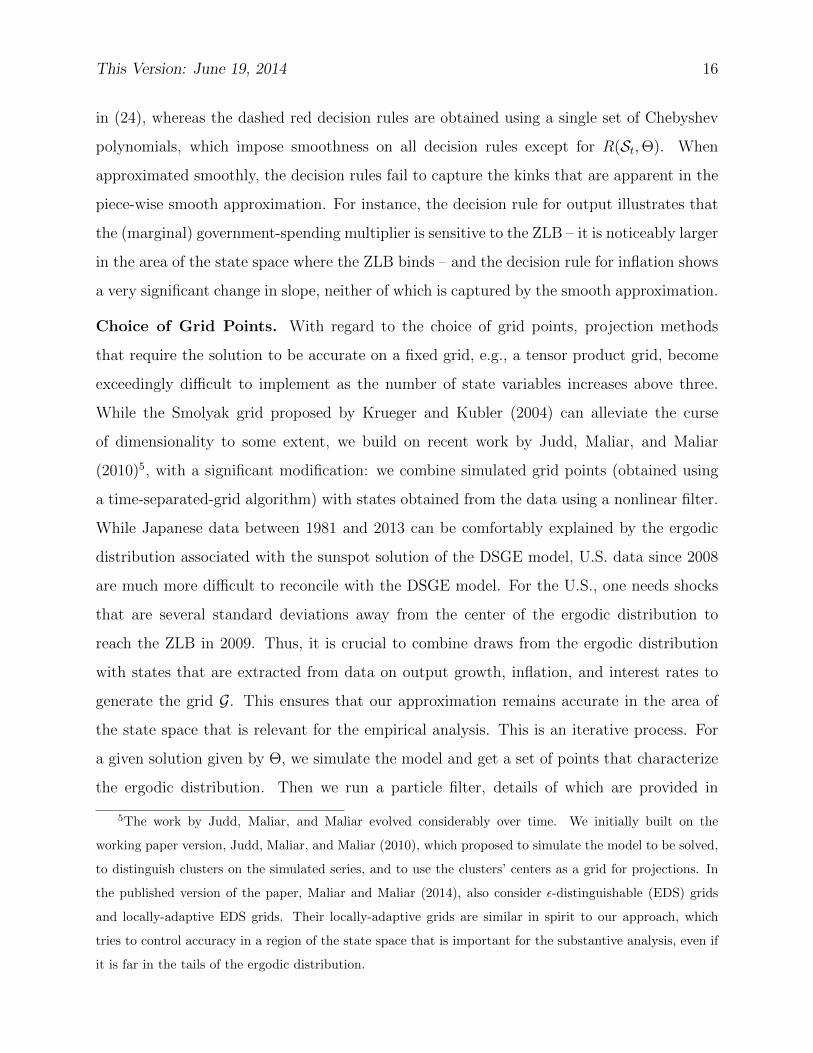
Choice of Grid Points. With regard to the choice of grid points, projection methods
that require the solution to be accurate on a fixed grid, e.g., a tensor product grid, become
exceedingly difficult to implement as the number of state variables increases above three.
While the Smolyak grid proposed by Krueger and Kubler (2004) can alleviate the curse
of dimensionality to some extent, we build on recent work by Judd, Maliar, and Maliar
(2010)5, with a significant modification: we combine simulated grid points (obtained using
a time-separated-grid algorithm) with states obtained from the data using a nonlinear filter.
While Japanese data between 1981 and 2013 can be comfortably explained by the ergodic
distribution associated with the sunspot solution of the DSGE model, U.S. data since 2008
are much more difficult to reconcile with the DSGE model. For the U.S., one needs shocks
that are several standard deviations away from the center of the ergodic distribution to
reach the ZLB in 2009. Thus, it is crucial to combine draws from the ergodic distribution
with states that are extracted from data on output growth, inflation, and interest rates to
generate the grid G. This ensures that our approximation remains accurate in the area of
the state space that is relevant for the empirical analysis. This is an iterative process. For
a given solution given by Θ, we simulate the model and get a set of points that characterize
the ergodic distribution. Then we run a particle filter, details of which are provided in
5The work by Judd, Maliar, and Maliar evolved considerably over time. We initially built on the
working paper version, Judd, Maliar, and Maliar (2010), which proposed to simulate the model to be solved,
to distinguish clusters on the simulated series, and to use the clusters’ centers as a grid for projections. In
the published version of the paper, Maliar and Maliar (2014), also consider ε-distinguishable (EDS) grids
and locally-adaptive EDS grids. Their locally-adaptive grids are similar in spirit to our approach, which
tries to control accuracy in a region of the state space that is important for the substantive analysis, even if
it is far in the tails of the ergodic distribution.

This Version: June 19, 2014 17
Section 5.4, to obtain the grid points which are consistent with the U.S. data since 2008.
Initialization of Θ. Recall that the sunspot equilibrium decision rules are obtained by
solving for Θ that minimizes the sum of squared residuals associated with (17) and (20) for
St ∈ G. We start the solution process by solving the model assuming p11 = p00 = 1, that
is, both sunspot regimes are absorbing states. This means, essentially, the decision rules
evaluated at st = 1 (st = 0) resemble those that would be obtained in the targeted-inflation
equilibrium (a minimal-state-variable deflation equilibrium). Once these decision rules are
accurately obtained, after some iterations of the simulate-filter-solve algorithm, we use them
as initial guesses of the decision rules of the full model with p11 < 1 and p00 < 1. When
the transition probabilities are nonzero, the agents anticipate regime changes to occur in the
future and this changes their decision rules. Still the initial guesses prove to be reasonably
accurate.6 We parameterize each f ij for i = 1, ..., 4 and j = π, E with 126 parameters for a
total of 1,008 elements in Θ and use M = 624 including the grid points from the ergodic
distribution and the filtered states. For a given set of filtered states and simulated grid, the
solution takes about two minutes on a single-core Windows-based computer using MATLAB.
The approximation errors are in the order of 10−4 or smaller, expressed in consumption units.
5 Quantitative Analysis
The data sets used in the empirical analysis are described in Section 5.1. In Section 5.2, we
estimate the parameters of the DSGE model for the U.S. and Japan using data from before
the economies reached the ZLB. These parameter estimates are the starting point for the
subsequent analysis. In Section 5.3, we compare the ergodic distributions of interest rates
and inflation under the parameter estimates obtained for the two countries. In Section 5.4
we show that the Japanese economy shifted to the deflation regime at the end of the 1990s
which triggered a long spell of zero nominal interest rates. The U.S., on the other hand,
stayed in the targeted-inflation regime after 2009 when interest rates reached the ZLB.
6We do the filtering iteration three times and within each iteration we do the simulation-solve iteration
five times. Further iterations do not change the results in any appreciable way.

This Version: June 19, 2014 18
Adverse demand shocks contributed to the low interest rates initially, and subsequently an
expansionary monetary policy kept interest rates at zero. We offer an interpretation of the
evolution of the estimated sunspot shocks in Section 5.5. Finally, Section 5.6 compares the
effects of an expansionary fiscal policy in the U.S. and Japan.
5.1 Data
The subsequent empirical analysis is based on real per-capita GDP growth, GDP deflator
inflation, and interest data for the U.S. and Japan. The U.S. interest rate is the federal
funds rate and for Japan we use the Bank of Japan’s uncollateralized call rate. Further
details about the data are provided in Appendix E. The time series are plotted in Figure 3.
The U.S. sample starts in 1984:Q1, after the start of the Great Moderation, whereas the
time series for Japan start in 1981:Q1. The vertical lines denote the end of the estimation
sample, which is 2007:Q4 for the U.S. and 1994:Q4 for Japan. We chose the endpoints for
the estimation sample such that the economies are unambiguously in the targeted-inflation
regime and away from the ZLB during the estimation period. For the U.S. the fourth quarter
of 2007 marks the beginning of the Great Recession, which was followed with a long-lasting
spell of zero interest rate starting in 2009. In Japan, short-term interest rates dropped below
50 basis points in 1995:Q4 and have stayed at or near zero ever since. A key feature of the
deflation regime in our model is that inflation rates are negative. While the U.S. experienced
only two quarters of negative inflation (2009:Q2 and Q3) and two quarters of inflation around
0.5% (2011:Q4 and 2013:Q2), inflation in Japan has been negative (or near zero) for most
quarters since 1995. These features of the data are important for the identification of the
sunspot regimes.
5.2 Model Estimation
We verified that the decision rules for the targeted-inflation regime in the region of the state
space for which the ZLB is far from being binding, are well approximated by the decision
rules obtained from a second-order perturbation solution of the DSGE model that ignores

This Version: June 19, 2014 19
Figure 3: Data
U.S. 1984-2013 Japan 1981-2013
Output Growth (%)
1985 1990 1995 2000 2005 2010−4
−2
0
2
4
Inflation (%)
1985 1990 1995 2000 2005 2010−5
0
5
Nominal Interest Rate (%)
1985 1990 1995 2000 2005 20100
5
10
Output Growth (%)
1985 1990 1995 2000 2005 2010−4
−2
0
2
4
Inflation (%)
1985 1990 1995 2000 2005 2010−5
0
5
Nominal Interest Rate (%)
1985 1990 1995 2000 2005 20100
5
10
Note: See Section 5.1 for the data definitions. The vertical red line in each figure show the end of theestimation sample. The yellow shading is explained in Section 5.4 and it shows the periods during whichP[{st = 1}|Y1:t] < 0.1 as assessed by the nonlinear filter.
the ZLB. Because the perturbation solution is much easier to compute and numerically more
stable than the global approximation to the sunspot equilibrium discussed in Section 4, we
end the estimation samples for the U.S. and Japan in 2007:Q4 and 1994:Q4, respectively. To
obtain posterior estimates of the DSGE model parameters we use a particle Markov chain
Monte Carlo approach along the lines of Fernandez-Villaverde and Rubio-Ramırez (2007)
and Andrieu, Doucet, and Holenstein (2010), which approximates the likelihood function
with a particle filter and embedds that approximation into a Metropolis-Hastings sampler.
The parameter estimates are in Table 1.7 A subset of the parameters were fixed prior to
7The prior distribution as well as the implementation of the posterior sampler are described in Ap-
This Version: June 19, 2014 20
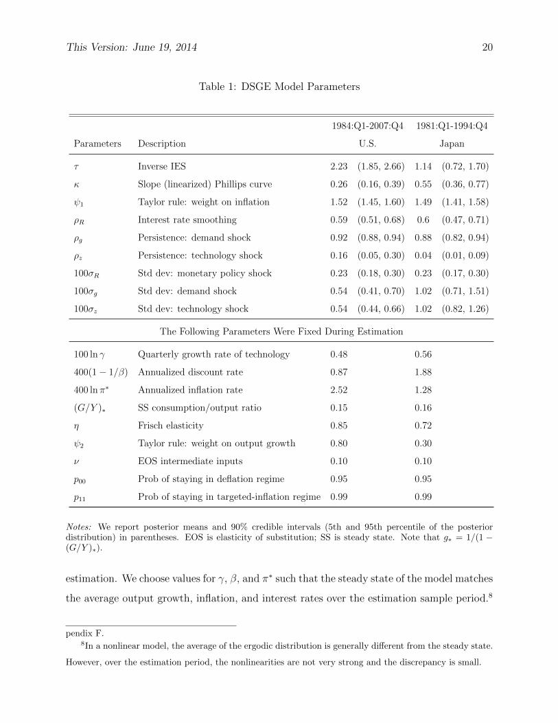
Table 1: DSGE Model Parameters
1984:Q1-2007:Q4 1981:Q1-1994:Q4
Parameters Description U.S. Japan
τ Inverse IES 2.23 (1.85, 2.66) 1.14 (0.72, 1.70)
κ Slope (linearized) Phillips curve 0.26 (0.16, 0.39) 0.55 (0.36, 0.77)
ψ1 Taylor rule: weight on inflation 1.52 (1.45, 1.60) 1.49 (1.41, 1.58)
ρR Interest rate smoothing 0.59 (0.51, 0.68) 0.6 (0.47, 0.71)
ρg Persistence: demand shock 0.92 (0.88, 0.94) 0.88 (0.82, 0.94)
ρz Persistence: technology shock 0.16 (0.05, 0.30) 0.04 (0.01, 0.09)
100σR Std dev: monetary policy shock 0.23 (0.18, 0.30) 0.23 (0.17, 0.30)
100σg Std dev: demand shock 0.54 (0.41, 0.70) 1.02 (0.71, 1.51)
100σz Std dev: technology shock 0.54 (0.44, 0.66) 1.02 (0.82, 1.26)
The Following Parameters Were Fixed During Estimation
100 ln γ Quarterly growth rate of technology 0.48 0.56
400(1− 1/β) Annualized discount rate 0.87 1.88
400 lnπ∗ Annualized inflation rate 2.52 1.28
(G/Y )∗ SS consumption/output ratio 0.15 0.16
η Frisch elasticity 0.85 0.72
ψ2 Taylor rule: weight on output growth 0.80 0.30
ν EOS intermediate inputs 0.10 0.10
p00 Prob of staying in deflation regime 0.95 0.95
p11 Prob of staying in targeted-inflation regime 0.99 0.99
Notes: We report posterior means and 90% credible intervals (5th and 95th percentile of the posteriordistribution) in parentheses. EOS is elasticity of substitution; SS is steady state. Note that g∗ = 1/(1 −(G/Y )∗).
estimation. We choose values for γ, β, and π∗ such that the steady state of the model matches
the average output growth, inflation, and interest rates over the estimation sample period.8
pendix F.8In a nonlinear model, the average of the ergodic distribution is generally different from the steady state.
However, over the estimation period, the nonlinearities are not very strong and the discrepancy is small.

This Version: June 19, 2014 21
The steady state government expenditure-to-output ratio is determined from national ac-
counts data. Since our sample does not include observations on labor market variables,
we fix the Frisch labor supply elasticity. Based on Rıos-Rull, Schorfheide, Fuentes-Albero,
Kryshko, and Santaeulalia-Llopis (2012), who provide a detailed discussion of parameter
values that are appropriate for DSGE models of U.S. data, we set η = 0.85 for the U.S.
Our value for Japan is based on Kuroda and Yamamoto (2008) who use micro-level data to
estimate labor supply elasticities along the intensive and extensive for males and females.
The authors report a range of values which we aggregated into η = 0.72.
We fix the value of ψ2 based on estimates of linearized DSGE models with an output-
growth rule.9 The parameter ν, which captures the elasticity of substitution between in-
termediate goods, is set to 0.1. It is essentially not separately identifiable from the price
adjustment cost parameter φ. Finally, we need to specify values for the transition proba-
bilities p00 and p11. These parameters determine the expected durations of staying in each
regime. Since there is no clear empirical observation to identify the transition probabilities,
we informally chose p00 = 0.95 and p11 = 0.99. These values make the deflation regime
(st = 0) less persistent than the targeted-inflation regime (st = 1) and imply unconditional
regime probabilities of 0.17 (st = 0) and 0.83 (st = 1), respectively.
For the remaining parameters, we report posterior mean estimates and 90% credible
intervals in Table 1. Overall, the estimates reported in the table are in line with the estimates
reported elsewhere in the literature. Most notable are the estimates of the degree of price
rigidity. Rather than reporting estimates for the adjustment cost parameter φ, we report
estimates for the implied slope of the New Keynesian Phillips curve in a linearized version
of the DSGE model (without ZLB constraint). This transformation takes the form κ =
τ(1− ν)/(νπ2∗φ). The slope estimate is 0.26 for the U.S. and 0.55 for Japan, implying fairly
flexible prices and relatively small real effects of unanticipated interest rate changes.10
9For Japan we use the average of the estimates from Ichiue, Kurozumi, and Sunakawa (2013) and
Fujiwara, Hirose, and Shintani (2011), which are 0.50 and 0.17 respectively. For the US we use the estimate
of Aruoba and Schorfheide (2013).10A survey of DSGE model-based New Keynesian Phillips curve is provided in Schorfheide (2008). Our
estimates fall within the range of the estimates obtained in the literature.

This Version: June 19, 2014 22
5.3 Equilibrium Dynamics
To understand how our model behaves at its ergodic distribution, we simulate a long sequence
of draws using the estimates for both countries. Figure 4 depicts contour plots of the ergodic
distributions of inflation and interest rates for the two countries in columns and for two
regimes in rows. In the contour plots each line represents one percentile with the outermost
line showing the 99th percentile. In each panel we show the data used to estimate the model
using black stars and the post-estimation data using green stars. There are a number of
noteworthy results. First, the ergodic distributions are centered near the respective steady
state values with the mean inflation when s = 1 slightly below π∗ and mean inflation when
s = 0 below 1/r. Second, focusing on the top row, the estimation data falls squarely inside
the ergodic distributions for s = 1 with only a few observations with high interest rates for
the U.S. Third, ZLB is not observed in the ergodic distribution for s = 1 for either country,
while in about 85% of observations feature the ZLB when s = 0 for both countries. This is
not surprising since the estimation samples of both countries cover a period of above-zero
interest rates and low macroeconomic volatility. Finally, deflation is very unlikely in the
U.S. when s = 1 with only a 1.1% probability, while in Japan this is much higher at 22.9%.
When s = 0, on the other hand, inflation is never positive.
To provide more details about the ergodic distribution, annualized output growth is
virtually identical across the two regimes for both countries. An important difference between
the two regimes is the correlation of (detrended) output and inflation. When s = 1, this
correlation is strongly positive – 0.83 for the U.S. and 0.73 for Japan – which is naturally
consistent with the data, albeit somewhat stronger. When s = 0, on the other hand, the
correlation becomes strongly negative, around −0.95 for both countries. This result is linked
to the findings of Eggertsson (2009) and Mertens and Ravn (2014), who show that positive
demand shocks may lead to a negative comovement of prices and output in the deflation
regime.11 Since the majority of fluctuations in our model is explained by the demand shock,
11More specifically, Mertens and Ravn (2014) show that the EE curve, which plots inflation versus output
using the relationship in (19) with necessary substitutions, has two segments, one downward sloping and
one upward sloping. If the equilibrium is in the upward-sloping portion, then a positive demand shock may
generate a decrease in inflation while increasing output.

This Version: June 19, 2014 23
Figure 4: Ergodic Distribution and Data
Inflation (%)
Nom
inal
Rat
e (%
)
−5 0 5
02
46
810
US (s=1)*
**
**
****
** * *
** ***
**
****
****
***
** ** **********
****** * ****** ** *** *
*****
**
**** *** ** **
**
**
****** ***
*
*
* *
* ** * ** **** *** ****** **
100% of ZLB obs
outside 99th
percentile
Inflation (%)
Nom
inal
Rat
e (%
)
−5 0 5
02
46
810
Japan (s=1)
*
** *** ** *
** * *** ****
*
*
****
* ** **** *
***
***
****
*
**
* *** *
** ** ****** *** * ** **** **** *** ** ** ** ** *** *** ** * **** *** * ** *** * ** ***** **** ** * *** * ** ** *
100% of ZLB obs
outside 99th
percentile
Inflation (%)
Nom
inal
Rat
e (%
)
−5 0 5
02
46
810
US (s=0)*
**
**
****
** * *
** ***
**
****
****
***
** ** **********
****** * ****** ** *** *
*****
**
**** *** ** **
**
**
****** ***
*
*
* *
* ** * ** **** *** ****** **
90% of ZLB obs
outside 99th
percentile
Inflation (%)
Nom
inal
Rat
e (%
)
−5 0 5
02
46
810
Japan (s=0)
*
** *** ** *
** * *** ****
*
*
****
* ** **** *
***
***
****
*
**
* *** *
** ** ****** *** * ** **** **** *** ** ** ** ** *** *** ** * **** *** * ** *** * ** ***** **** ** * *** * ** ** *
29% of ZLB obs
outside 99th
percentile
Notes: In each panel we report the joint probability density function (kernel density estimate) of annualizednet interest rate and inflation, represented by the contours. Black stars show the data used in estimation.Green stars show the rest of the data.
this delivers the negative correlation.12
The focus of this paper is not normative, but it is worth mentioning that the deflationary
regime is not necessarily “bad” in terms of welfare. Average consumption across the two
regimes are identical and the volatility of consumption is 24% higher in the deflationary
regime. The distance between actual and desired inflation (0%) is larger in the deflationary
regime relative to the targeted-inflation regime, which means the adjustment costs will be
larger. These observations would imply a lower welfare for the deflationary regime. However,
12We show impulse responses for the U.S. economy in Appendix G.

This Version: June 19, 2014 24
the interest rate is much closer, in fact most of the time exactly equal to zero (the Friedman
rule) and thus the welfare cost due to holding money is much smaller. We leave a full-blown
normative analysis along the lines of Aruoba and Schorfheide (2011) to future work.
5.4 Evidence For the Deflation Regime in the U.S. and Japan
The DSGE model has a nonlinear state-space representation of the form
dt = Ψ(xt) + νt
xt = Fst(xt−1, εt) (25)
P{st = 1} =
(1− p00) if st−1 = 0
p11 if st−1 = 1
Here dt is the 3× 1 vector of observables consisting of output growth, inflation, and nominal
interest rates and D1:t is the sequence {d1, . . . , dt}. The vector xt stacks the continuous state
variables, which are given by xt = [Rt, yt, yt−1, zt, gt, At]′, and st ∈ {0, 1} is the Markov-
switching process. The first equation in (25) is the measurement equation, where νt ∼
N(0,Σν) is a vector of measurement errors. The second equation corresponds to the law of
motion of the continuous state variables. The vector εt ∼ N(0, I) stacks the innovations εz,t,
εg,t, and εR,t. The functions F0(·) and F1(·) are generated by the model solution procedure
described in Section 4. The third equation represents the law of motion of the Markov-
switching process. Conditioning on the posterior mean estimates obtained in Section 5.2,
we now use a sequential Monte Carlo filter (also known as the particle filter)13 to extract
estimates of the sunspot shock process st, and the latent state xt.
The main result is presented in Figure 5, which depicts the filtered probabilities P[st =
1|D1:t] of being in the targeted-inflation regime. According to our estimates, the experience
of the U.S. and Japan was markedly different. With the exception of 2011:Q4, when the
probability of the deflation regime increased to about 70%, the U.S. has been in the targeted-
inflation regime. In 2009:Q2, the probability of the deflation regime is small, but non-zero,
13This filter is a more elaborate version of the filter that underlies the estimation in Section 5.2. It is
described in detail in Appendix H. A recent survey of sequential Monte Carlo methods is provided by Creal
(2012).

This Version: June 19, 2014 25
Figure 5: Filtered Probability of Targeted-Inflation Regime
U.S. JapanProb (s=1)
1985 1990 1995 2000 2005 20100
0.2
0.4
0.6
0.8
1Prob (s=1)
1985 1990 1995 2000 2005 20100
0.2
0.4
0.6
0.8
1
Notes: The solid red vertical bar indicates the end of the estimation sample. The shaded area indicates timeperiods for which the filtered probability for the targeted-inflation regime falls below 10%.
vindicating Bullard’s (2010) concern of a shift to the deflationary regime. Japan, on the other
hand, experienced a switch to the deflation regime in 1999:Q2, and, except for the period
from 2008:Q4 to 2009:Q3, has stayed in the deflation regime.14 Recall from Figure 3 that the
U.S. interest rates have been essentially zero since 2009:Q1, whereas in Japan interest rates
have been below 50 basis points since 1995:Q4, and essentially zero since 1999:Q1. While
in the case of the U.S. the ZLB spell is interpreted as evidence in favor of the targeted-
inflation regime, for Japan it is attributed toward a shift into the deflation equilibrium. The
key reason for this difference is the behavior of inflation. The U.S. experienced only three
quarters of low or negative inflation rates, whereas prices have been on average falling for
many years in Japan. The ergodic distributions depicted in Figure 4 highlight that the
deflation regime not only implies that interest rates are close to zero, it also implies that
inflation is negative with very high probability. Accordingly, it shows that none of the ZLB
observations fall inside 99% of the ergodic distribution for the targeted-inflation refime for
14A large decline in oil prices lead to a decrease in the import deflator which in turn generated a large
jump in the GDP deflator to about 6% in 2008:Q4. If we remove this observation, then the temporary switch
to the targeted-inflation regime vanishes. If we use CPI instead of the GDP deflator as our price measure,
we find a long spell of the deflation regime from 2000 to 2008 as well as a subsequent shorter spell.

This Version: June 19, 2014 26
either country, while about 70% of ZLB observations for Japan are well inside the ergodic
distribution for the deflation regime.
In the absence of a switch to the deflation regime, the U.S. reaches the ZLB in response
to very large negative innovations (greater than 2 standard deviations) to the latent demand
shock process gt. Since the DSGE model has a fairly strong mean reversion, a sequence of
expansionary monetary policy shocks are necessary to prevent the nominal interest rate from
rising. In the absence of these monetary policy shocks, U.S. nominal interest rates would
have averaged 1.3% whereas average inflation would have been 0.4% instead of 1.6% after
2009. In Japan, the switch to the deflation regime pushed the economy toward the ZLB.
While interest rates are close to zero in the deflation regime, Figure 4 shows that inflation
rates should be less than -2.5% with very high probability. The average inflation rate between
1999 and 2008 is about -1.3%. The model rationalizes the relatively low observed deflation
with a sequence of demand shock innovations that is on average slightly negative. Recall
that in the deflation regime a negative εg,t tends to raise inflation.
5.5 Interpretation of Results
From the perspective of our model both the U.S. and the Japanese economy experienced a
sequence of adverse demand shocks that lead to a fall in interest rates.15 In the U.S. it was
the financial crisis that unfolded during 2008 and peaked in the fourth quarter. For Japan
some of the obvious culprits are the burst of the housing bubble (1992:Q1), the East-Asian
/ Korean crises (1997) and the Russian Financial Crisis (1998Q3). Following these events,
short-term interest rates have been zero both in the U.S. and Japan. The key finding of
our empirical analysis is that the two countries stayed at the ZLB for very different reasons.
Japan experienced a switch of the sunspot variable st from the targeted-inflation regime to
the deflation regime in 1999:Q2. The Japanese economy essentially stayed in the deflation
regime until the end of our sample in 2013. For the U.S., on the other hand, there is no strong
evidence of a switch to the deflation regime. A change in the sunspot regime means that the
agents in the economy coordinated their expectations and actions based on some extraneous
15The filtered εg,t shocks are plotted in Figure A-4 in the Appendix.

This Version: June 19, 2014 27
Figure 6: 10-Year Inflation Expectations
0.0
0.5
1.0
1.5
2.0
2.5
3.0
90 92 94 96 98 00 02 04 06 08 10 12
JapanUS
Inflation Expectations - 10 Year Ahead
ZLB ZLB
Notes: Units are annualized percentage. Vertical lines show the quarter where interest rates fall to the ZLBin each country.
information. While this information is not directly observed by us, we will compare aspects
of monetary policy in Japan and the U.S. that may have contributed to agents’ expectation
formation and, through the lens of our model, determined whether a regime switch occurred.
Mechanically, st is an exogenous process in our model and agents’ decision rules and
expectations about the future are indexed by st. Since a switch in st triggers changes in
expectations, we can interpret the sunspot shock also as an exogenous shock to expectations.
In Figure 6 we plot 10-year inflation expectations for Japan and the U.S. starting give years
prior to each country’s respective ZLB episode. For Japan we use the Consensus Forecasts
and for the U.S. we use the results from Aruoba (2014), which are based on surveys. The
vertical lines in the figure depict the start of the ZLB episode of the two countries. For the
U.S., long-run inflation expectations simply do not move during or after the financial crisis
and they show small fluctuations around 2.3%. For Japan, the expectations are around 2.5%

This Version: June 19, 2014 28
prior to the burst of the housing price bubble and they gradually decline to 0.5% by 2003.
Of course the realized quarterly or annual inflation is consistently negative throughout this
period as well. Thus, the evidence in Figure 6 is consistent with the interpretation that
Japan experienced a shock to inflation expectations whereas the U.S. did not.
Inflation expectations are closely tied to expectations about future monetary policy. In
Japan the policy rate was pushed to the ZLB in 1999, but any further action such as com-
mitting to a particular target or quantitative easing (QE) was expressly ruled out. A speech
by the then-governor Hayami (1999) explains that this policy is in effect “until deflationary
concerns subside” (Page 1). He then goes on to imply that rates may go up before inflation
becomes positive, if the Bank of Japan decides that price stability may be at jeopardy at
some future point in time. In fact, the Bank of Japan increased its policy rate in August
2000 based on inflation concerns, even though prices have been continuously falling for many
quarters. He also dismisses the need for QE arguing that a cut in the interest rates achieves
what QE can achieve, no more, no less. When QE was finally implemented in 2001, the
policy wasn’t explained clearly and previous claims by bank officials about the perceived
ineffectiveness of QE was not refuted. To sum up, as Ito and Mishkin (2006), who provide
and excellent (and critical) summary of the actions taken by the Bank of Japan and the
Japanese government, put it: “The Bank of Japan had a credibility problem, particularly
under the Hayami Regime [1998-2003], in which the markets and the public did not expect
the Bank of Japan to pursue expansionary monetary policy in the future, which would en-
sure that deflation would end. These mistakes in the management of expectations are a key
reason why Japan found itself in a deflation that it is finding very difficult to get out of”
(Page 165).
The actions of U.S. policymakers following the financial crisis of 2008 contrast greatly
with the actions of the Bank of Japan. The Federal Reserve and in general policy makers
in the U.S. reacted to the financial crisis very forcefully, using unconventional tools early
on. By the end of 2008 as the federal funds rate target was brought to near-zero levels,
several rounds of large-scale asset purchase policies were implemented to provide liquidity
to the banking system and lower long-term interest rates. Moreover, the Federal Reserve

This Version: June 19, 2014 29
implemented a policy of “forward guidance.” Starting from the December 2008 policy an-
nouncement, the Federal Reserve made its intention of keeping the federal funds rate near
zero for an extended period of time very clear. The December 2008 press release includes the
following statement: “The committee anticipates that weak economic conditions are likely to
warrant exceptionally low levels of the federal funds rate for some time.” The statement was
strengthened by changing “some time” to “an extended period” three months later. Starting
in August 2011, the Federal Reserve was even more specific, providing explicit time frames
for the low rates.
Thus, a plausible interpretation of our empirical findings is the following. In the U.S.
the expansionary unconventional monetary policies of the Federal Reserve kept inflation ex-
pectations anchored and prevented a switch to the deflation regime. The Bank of Japan, on
the other hand, did not convince the public that it would pursue an aggressive expansionary
monetary policy, which triggered an adverse shock to inflation expectations and moved the
economy into the deflation regime. Ueda (2011) provides a very thorough review of the poli-
cies used in the U.S. and Japan and he concludes that “the entrenched nature of deflationary
expectations, however, seems to have prevented [the zero interest rate and QE policies to
increase inflation expectations on a significant scale for a sustained period]. Unfortunately,
the Japanese economy seems to be trapped in an ‘equilibrium’ whereby only exogenous forces
generate movements to a better equilibrium with a higher rate of inflation” (Page 20). This,
of course, is precisely the point we show formally in this paper.
5.6 Policy Experiments
During their respective ZLB episodes, both Japan and the U.S. engaged in unprecedented fis-
cal and monetary interventions. The U.S. enacted the American Recovery and Reinvestment
Act (ARRA) in February 2009, which consisted of various fiscal interventions, a significant
part of which was government spending. Similarly, there have been numerous fiscal programs
in Japan starting in 1998, some of which were explicitly aimed at dealing with various local
shocks (e.g., the 2011 earthquake) or global shocks (e.g., the global financial crisis), and
starting in 2010 with deflation. We provide a summary of these programs in Table A-1. All

This Version: June 19, 2014 30
of these policies were aimed at increasing real economic activity, increasing inflation from
deflationary levels (or preventing it to go there), or both. In this section, our main goal is to
demonstrate how these fiscal policies may have drastically different effects on the economy,
depending on whether a shift to the deflation regime or an adverse sequence of shocks in the
targeted-inflation regime keeps the economy near the ZLB.
The recent literature has emphasized that the effects of expansionary fiscal policies on
output may be larger if the economy is at or near the ZLB. In the absence of the ZLB, a
typical interest rate feedback rule implies that the central bank raises nominal interest rates
in response to rising inflation and output caused by an increase in government spending. This
monetary contraction raises the real interest rate, reduces private consumption, and overall
dampens the stimulating effect of the fiscal expansion. If the economy is at the ZLB, the
expansionary fiscal policy is less likely to be accompanied by a rise in interest rates because
the feedback portion of the policy rule tends to predict negative interest rates. Without a
rising nominal interest rate, the increase in inflation that results from the fiscal expansion
reduces the real rate. In turn, current-period demand is stimulated, amplifying the positive
effect on output. In fact, the decision rules depicted in Figure 2 show that when the ZLB
starts to bind, the response of output to an increase in government spending is larger, and
consumption goes up.16
5.6.1 Details of the Policy Experiments
Due to the nonlinearity of our DSGE model, the effect of policy interventions captured by
impulse response functions depend on the initial state of the economy. Rather than condi-
tioning on one particular time period, we average results for several periods. We distinguish
16To be clear, the typical exercise in the literature is not a standard impulse response analysis. The
analysis assumes the existence of a very large impulse other than the policy impulse being considered that
affects the economy and causes the ZLB to bind. This shock is assumed to be large enough so that even
after the policy impulse, which would have increased the nominal interest rate, the ZLB continues to bind.
As an example, Fernandez-Villaverde, Gordon, Guerron-Quintana, and Rubio-Ramırez (2012) uses an eight-
standard-deviation shock to the discount factor to keep the economy at the ZLB.

This Version: June 19, 2014 31
between ZLB periods (2009:Q1 to 2011:Q1 for the U.S. and 1999:Q2 to 2005:Q2 for Japan)
and non-ZLB periods (1984:Q1 to 2005:Q2 for the U.S. and 1981:Q2 to 1991:Q2 for Japan).
The policy effect for a particular quarter is computed as follows. Suppose that we condi-
tion on the state of the economy in period t−1 and track the economy for H periods. First we
compute P[st+h = 1|D1:t+h], where D1:t+h denotes the sequence of observations d1, . . . , dt+h
for h = 0, 1, . . . , H. If this probability exceeds 10% we set st+h = 1; otherwise we set
st+h = 0. Second, we compute an estimate of the remaining states: xt−1 = E[xt−1|st, D1:t]
as well as estimates of the shocks εi,t+h = E[εi,t+h|st:t+h, D1:t+h] for i = g, r, z. Third, we
compute the non-intervention path by iterating the state-transition equations forward based
on the filtered shocks εi,t+h. By construction, the non-intervention path reproduces the ac-
tual data. Fourth, we generate the intervention paths for consumption, output, inflation
and interest rates (signified by an I superscript) by setting εIg,t = εg,t + f (f represents the
size of the fiscal intervention), εIr,t = εr,t, εIz,t = εz,t, and εIi,t+h = εi,t+h for i = g, r, z and
h > 0 and iterating the state-transition equation forward based on the εIi,t+h’s. We also
compute cumulative government spending multipliers for the first H periods following the
intervention:
µH =
∑Hh=0(Y
It+h − Yt+h)∑H
h=0(GIt+h −Gt+h)
. (26)
Note that according to our timing convention H = 0 corresponds to the multiplier upon
impact of the shock.
After conducting the same policy intervention for every period t in the ZLB (non-ZLB)
period, we record the median and various percentiles of the government spending multiplier
and the difference between the paths with and without the intervention. For the ZLB period
this methodology conditions on the economy being at the ZLB, integrating out the conditions
that cause the economy to stay at the ZLB.
We consider two policy experiments, beginning with a pure fiscal expansion where g
increases by 1.5σg. This is a reasonably large intervention, which is also in line with the
actual policy interventions in these countries.17 The second experiment couples the same
17For example, when we looked at the funding for federal contracts, grants, and loans portion of ARRA as
disbursed in the first two quarters of the program, which amounts to just over 1% of GDP, this is equivalent

This Version: June 19, 2014 32
fiscal intervention with a commitment by the central bank to keep interest rates at or near
the ZLB. This central bank intervention is implemented using a sequence of unanticipated
monetary policy shocks εR,t.18 To avoid implausibly large interventions, we choose these
shocks such that they are no larger than two standard deviations in absolute value, and the
interest-rate intervention is no larger than one percentage point in annualized terms in any
quarter. Thus, we implicitly assume that the central bank would renege on a policy to keep
interest rates near zero for an extended period of time in states of the world in which output
growth and/or inflation turn out to be high. For each experiment, we report the paths of
key variables following the policy interventions, as well as cumulative government spending
multiplier. Appendix D.2 provides some more details.
5.6.2 Pure Fiscal Policy Intervention
The impulse responses for the fiscal-only policy intervention for the U.S. is presented in
Figure 7 and the multipliers for all policy experiments are summarized in Table 2. In each
panel of Figure 7 the blue line indicates the response of the economy during non-ZLB periods
and the red line shows the response of the economy during the ZLB periods. Recall that in
the U.S. the ZLB is reached within the targeted-inflation regime by large adverse demand
shocks. Even though these shocks lie far in the tails of the ergodic distribution, the response
of the economy in the ZLB period closely resembles the response during non-ZLB periods,
which in turn is the “standard” response to a government spending shock in a New Keynesian
DSGE model: on impact output goes up by slightly less than 0.5% and inflation increases by
about 25 basis points. As a result, the central bank raises the nominal interest rate by over
75 basis points, which means roughly a 50 basis point increase in the real interest rate. This
reduces consumption by over 0.35%, which is the standard crowding-out effect of government
spending. All of these changes yield a fiscal multiplier of 0.62 on impact, which goes up to
to a g shock of size 1.4σg. Table A-1 also shows that there were sizable fiscal programs in Japan, some of
which were upwards of 3% of GDP.18A detailed discussion about the advantages and disadvantages of using unanticipated versus anticipated
monetary policy shocks to generate predictions conditional on an interest rate path is provided in Del Negro
and Schorfheide (2012).
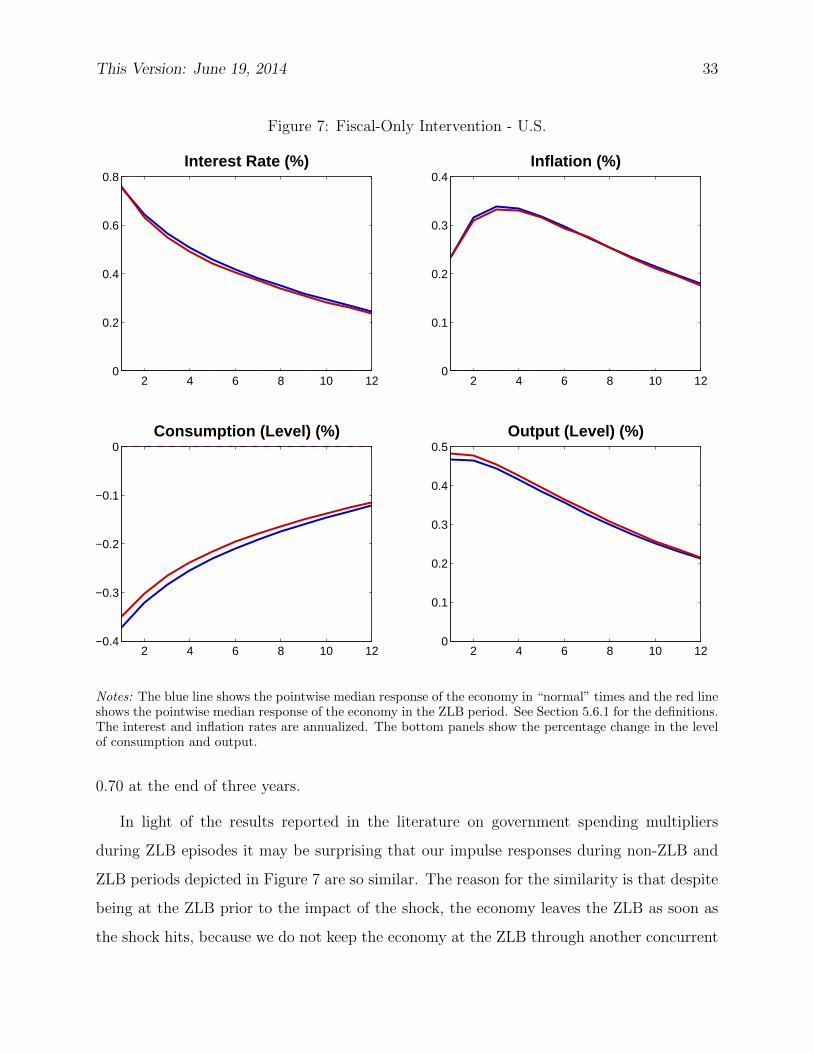
This Version: June 19, 2014 33
Figure 7: Fiscal-Only Intervention - U.S.
Interest Rate (%)
2 4 6 8 10 120
0.2
0.4
0.6
0.8Inflation (%)
2 4 6 8 10 120
0.1
0.2
0.3
0.4
Consumption (Level) (%)
2 4 6 8 10 12−0.4
−0.3
−0.2
−0.1
0Output (Level) (%)
2 4 6 8 10 120
0.1
0.2
0.3
0.4
0.5
Notes: The blue line shows the pointwise median response of the economy in “normal” times and the red lineshows the pointwise median response of the economy in the ZLB period. See Section 5.6.1 for the definitions.The interest and inflation rates are annualized. The bottom panels show the percentage change in the levelof consumption and output.
0.70 at the end of three years.
In light of the results reported in the literature on government spending multipliers
during ZLB episodes it may be surprising that our impulse responses during non-ZLB and
ZLB periods depicted in Figure 7 are so similar. The reason for the similarity is that despite
being at the ZLB prior to the impact of the shock, the economy leaves the ZLB as soon as
the shock hits, because we do not keep the economy at the ZLB through another concurrent

This Version: June 19, 2014 34
Table 2: Cumulative Fiscal Multipliers
U.S. Japan
H 0 3 7 11 0 3 7 11
Ergodic Distribution
Fiscal 0.62 0.67 0.68 0.70 0.58 0.56 0.56 0.56
ZLB Episode
Fiscal 0.62 0.67 0.69 0.70 0.47 0.46 0.46 0.46
Fiscal and Monetary 1.16 1.23 1.25 1.24 0.47 0.46 0.46 0.46
Note: The multiplier is defined in (26).
shock.19 As soon as the economy exits the ZLB, the additional channel that boosts the
output response through the reduction of the real interest rate is absent. A second reason
for the relatively small multiplier is the Frisch labor supply elasticity of η = 0.85. The
multiplier is increasing in η and almost reaches one if η = ∞, i.e., preferences are quasi
linear.20
For Japan a very different picture emerges. Results are presented in Figure 8. As we
discussed in Section 5.4, Japan remains at the deflationary regime (st = 0) throughout the
ZLB period and thus behaves very differently relative to the non-ZLB period. In particular,
as a result of the fiscal intervention, the inflation rate falls sharply by 100 basis points
in the ZLB period, while it increases, as the conventional wisdom would suggest, during
non-ZLB periods. This decline in inflation is large enough to wipe out any desire for the
central bank to increase the interest rate and thus the economy stays at the ZLB. A constant
interest rate along with a decline in inflation increases the real interest rate and this depresses
19When Fernandez-Villaverde, Gordon, Guerron-Quintana, and Rubio-Ramırez (2012) conduct a similar
exercise without forcing the ZLB, they get a multiplier around 0.5. See footnote 16 for further details.20Christiano, Eichenbaum, and Rebelo (2011) obtains multipliers larger than one even away from the
ZLB when they use a utility function where consumption and leisure are close complements so that when
employment increases in response to a government spending shock, so does consumption.

This Version: June 19, 2014 35
Figure 8: Fiscal-Only Intervention - Japan
Interest Rate (%)
2 4 6 8 10 120
0.2
0.4
0.6
0.8
1Inflation (%)
2 4 6 8 10 12−1.5
−1
−0.5
0
0.5
1
Consumption (Level) (%)
2 4 6 8 10 12−1
−0.8
−0.6
−0.4
−0.2
0Output (Level) (%)
2 4 6 8 10 120
0.2
0.4
0.6
0.8
1
Notes: The blue line shows the pointwise median response of the economy in “normal” times and the redline shows the pointwise median response of the economy in the ZLB period. The shaded areas are theupper and lower 20% percentiles of the distribution of responses. See Section 5.6.1 for the definitions. Theinterest and inflation rates are annualized. The bottom panels show the percentage change in the level ofconsumption and output.
consumption further. Note that this is the channel emphasized in the literature as being
responsible for increasing the multiplier at the ZLB but working in exactly the opposite
direction since inflation falls. At the end, output still goes up as a result of this intervention
but the increase is reduced by about 0.15%, which is almost a fifth of the response during
the non-ZLB periods. In terms of multipliers, the impact multiplier in normal times is 0.58
and it is 0.47 in the ZLB period.

This Version: June 19, 2014 36
5.6.3 Combined Fiscal and Monetary Policy Intervention
We now combine the fiscal intervention with the promise of the central bank to keep rates at
or near the ZLB. We only consider the ZLB period for this exercise since in “normal” times
the interest rate is far from the ZLB and an expansionary monetary policy that pushes the
interest rate all the way to zero would be unrealistic. In Japan the interest rate remains zero
after the fiscal-only intervention, thus we consider the combined fiscal and monetary policy
only for the U.S. The results are reported in Figure 9.
In all of the twelve quarters under consideration, the central bank manages to pull the
interest rate all the way to the ZLB, despite the increasing urge not to do so due to higher
inflation and output responses. As a result, the output response exactly doubles to almost
1%, a large fraction of which comes from the smaller decline in consumption, since the channel
through the real interest rate is in effect. The impact multiplier increases by 87% and after
three years the multiplier is still 77% larger. All of this shows that, unlike Japan which
is in the deflationary regime, when the economy is at the ZLB because of adverse demand
shocks while at the targeted-inflation regime, the monetary stimulus we consider provides a
very large additional boost to the fiscal intervention. In this regard, our empirical findings
are consistent with earlier results reported in the literature. However, our interpretation is
different. The reason that the fiscal intervention has a large effect is because an expansionary
monetary policy keeps interest rates at zero. This interpretation is consistent with the filtered
monetary policy shocks shown in Appendix H.5. On average, these shocks have been negative
after 2009, meaning that from an ex-post perspective, monetary policy, through the lens of
our model, has been expansionary in the aftermath of the Great Recession.
6 Conclusion
We solve a small-scale New Keynesian DSGE model with the ZLB constraint and Markov
sunspot shocks that can move the economy between a targeted-inflation regime and a de-
flation regime. An economy may stay at or near the ZLB either by successive exogenous
shocks (e.g. adverse demand or technology shocks or expansionary monetary policy shocks)
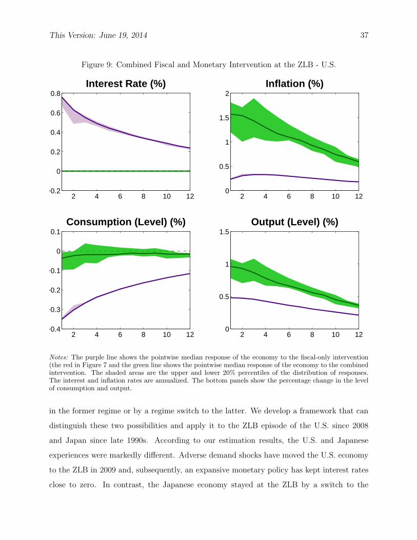
This Version: June 19, 2014 37
Figure 9: Combined Fiscal and Monetary Intervention at the ZLB - U.S.
Interest Rate (%)
2 4 6 8 10 12−0.2
0
0.2
0.4
0.6
0.8Inflation (%)
2 4 6 8 10 120
0.5
1
1.5
2
Consumption (Level) (%)
2 4 6 8 10 12−0.4
−0.3
−0.2
−0.1
0
0.1Output (Level) (%)
2 4 6 8 10 120
0.5
1
1.5
Notes: The purple line shows the pointwise median response of the economy to the fiscal-only intervention(the red in Figure 7 and the green line shows the pointwise median response of the economy to the combinedintervention. The shaded areas are the upper and lower 20% percentiles of the distribution of responses.The interest and inflation rates are annualized. The bottom panels show the percentage change in the levelof consumption and output.
in the former regime or by a regime switch to the latter. We develop a framework that can
distinguish these two possibilities and apply it to the ZLB episode of the U.S. since 2008
and Japan since late 1990s. According to our estimation results, the U.S. and Japanese
experiences were markedly different. Adverse demand shocks have moved the U.S. economy
to the ZLB in 2009 and, subsequently, an expansive monetary policy has kept interest rates
close to zero. In contrast, the Japanese economy stayed at the ZLB by a switch to the

This Version: June 19, 2014 38
deflation regime in 1999. While both economies were affected by adverse demand shocks
that pushed them to the ZLB, we argue that the U.S. economy did not experience a regime
switch due to the strong and committed response of the Federal Reserve that coordinated
private inflation expectations near its target. The Bank of Japan, on the other hand, was
unable to coordinate expectations, perhaps due to its weak reaction to the adverse shocks
early on, and the regime switch took place.
The U.S. and Japan’s experiences of moving to the ZLB have drastically different policy
implications. Fiscal multipliers are about 20% smaller in the deflationary regime, despite
the economy remaining at the ZLB. While a commitment by the central bank to keep rates
near the ZLB doubles the fiscal multipliers in the targeted-inflation regime (U.S.), it has no
effect in the deflation regime (Japan). Moreover, our results show that Japan experienced
persistent deflation because of the switch to the deflationary regime and this may explain
why numerous fiscal policies enacted in Japan in the last 15 years were not able generate
positive inflation.
Solving for the sunspot equilibrium is computationally challenging. We leave extensions
to larger DSGE models and equilibria in which the regime shifts are triggered by fundamental
shocks to future research. The latter will be important in formalizing the idea we explored
in this paper where central bank’s actions other than their interest rate decisions may help
coordinate private expectations and induce a switch in regimes. Finally, in future work we
plan to conduct a normative analysis in the sunspot equilibrium.
References
An, S., and F. Schorfheide (2007): “Bayesian Analysis of DSGE Models,” Econometric
Reviews, 26(2-4), 113–172.
Andrieu, C., A. Doucet, and R. Holenstein (2010): “Particle Markov Chain Monte
Carlo Methods,” Journal of the Royal Statistical Society Series B, 72(3), 269–342.
Armenter, R. (2014): “The Perils of Nominal Targets,” Manuscript, Federal Reserve Bank
of Philadelphia.

This Version: June 19, 2014 39
Aruoba, S. Boragan, L. B., and F. Schorfheide (2013): “Assessing DSGE Model
Nonlinearities,” Manuscript, University of Maryland and University of Pennsylvania.
Aruoba, S. B. (2014): “A Survey-Based Term Structure of Inflation Expectations,”
Manuscript, University of Maryland.
Aruoba, S. B., and F. Schorfheide (2011): “Sticky Prices versus Monetary Frictions:
An Estimation of Policy Trade-Offs,” American Economic Journal: Macroeconomics, 3(1),
60–90.
Benhabib, J., S. Schmitt-Grohe, and M. Uribe (2001a): “Monetary Policy and Mul-
tiple Equilibria,” The American Economic Review, 91(1), 167–186.
Benhabib, J., S. Schmitt-Grohe, and M. Uribe (2001b): “The Perils of Taylor Rules,”
Journal of Economic Theory, 96, 40–69.
Braun, R. A., L. M. Korber, and Y. Waki (2012): “Some Unpleasant Properties
of Log-Linearized Solutions When the Nominal Rate Is Zero,” Federal Reserve Bank of
Atlanta Working Paper Series.
Bullard, J. (2010): “Seven Faces of ‘The Peril’,” Federal Reserve Bank of St. Louis Review,
92(5), 339–352.
Cass, D., and K. Shell (1983): “Do Sunspots Matter?,” Journal of Political Economy,
91(2), 193–227.
Christiano, L., M. Eichenbaum, and S. Rebelo (2011): “When Is the Government
Spending Multiplier Large?,” Journal of Political Economy, 119(1), 78–121.
Cochrane, J. (2013): “The New-Keynesian Liquidity Trap,” Manuscript, Chicago Booth
School of Business.
Creal, D. (2012): “A Survey of Sequential Monte Carlo Methods for Economics and
Finance,” Econometric Reviews, 31(3), 245–296.

This Version: June 19, 2014 40
Del Negro, M., and F. Schorfheide (2012): “DSGE Model Based Forecasting,” in
Handbook of Economic Forecasting, ed. by G. Elliot, and A. Timmermann, vol. 2, p.
forthcoming. Elsevier.
Eggertsson, G. B. (2009): “What Fiscal Policy Is Effective at Zero Interest Rates?,”
Federal Reserve Bank of New York Staff Reports, no. 402, 402.
Eggertsson, G. B., and M. Woodford (2003): “The Zero Bound on Interest Rates and
Optimal Monetary Policy,” Brookings Papers on Economic Activity, 2003(1), 139–211.
Fernandez-Villaverde, J., G. Gordon, P. Guerron-Quintana, and J. F. Rubio-
Ramırez (2012): “Nonlinear Adventures at the Zero Lower Bound,” National Bureau of
Economic Research Working Paper.
Fernandez-Villaverde, J., and J. F. Rubio-Ramırez (2007): “Estimating Macroeco-
nomic Models: A Likelihood Approach,” Review of Economic Studies, 74(4), 1059–1087.
Fujiwara, I., Y. Hirose, and M. Shintani (2011): “Can News Be a Major Source of
Aggregate Fluctuations? A Bayesian DSGE Approach,” Journal of Money, Credit and
Banking, 43(1), 1–29.
Gust, C., D. Lopez-Salido, and M. E. Smith (2012): “The Empirical Implications of
the Interest-Rate Lower Bound,” Manuscript, Federal Reserve Board.
Hayami, M. (1999): “Mr. Hayami Discusses the Bank of Japan’s Thinking Behind the Cur-
rent Zero Interest Rate Policy,” http://www.bis.org/review/r990708a.pdf, Accessed
June 1, 2014.
Hursey, T., and A. L. Wolman (2010): “Monetary Policy and Global Equilibria in a
Production Economy,” Economic Quarterly, 96(4), 317–337.
Ichiue, H., T. Kurozumi, and T. Sunakawa (2013): “Inflation Dynamics And Labor
Market Specifications: A Bayesian Dynamic Stochastic General Equilibrium Approach
For Japan’S Economy,” Economic Inquiry, 51(1), 273–287.

This Version: June 19, 2014 41
Ireland, P. N. (2004): “Money’s Role in the Monetary Business Cycle,” Journal of Money,
Credit and Banking, 36(6), 969–983.
Ito, T., and F. S. Mishkin (2006): “Two Decades of Japanese Monetary Policy and the
Deflation Problem,” in Monetary Policy under Very Low Inflation in the Pacific Rim, ed.
by T. Ito, and A. Rose, vol. NBER-EASE, Volume 15, pp. 131–202. University of Chicago
Press.
Judd, K., L. Maliar, and S. Maliar (2010): “A Cluster-Grid Projection Method:
Solving Problems with High Dimensionality,” NBER Working Paper, 15965.
Judd, K. L. (1992): “Projection Methods for Solving Aggregate Growth Models,” Journal
of Economic Theory, 58(2), 410 – 452.
Kitagawa, G. (1996): “Monte Carlo Filter and Smoother for Non-Gaussian Nonlinear
State Space Models,” Journal of Computational & Graphical Statistics, 5, 1–25.
Krueger, D., and F. Kubler (2004): “Computing Equilibrium in OLG Models with
Production,” Journal of Economic Dynamics and Control, 28, 1411–1436.
Kuroda, S., and I. Yamamoto (2008): “Estimating The Frisch Labor Supply Elasticity
in Japan,” Journal of the Japanese and International Economies, 22(4), 566–585.
Lubik, T. A., and F. Schorfheide (2004): “Testing for Indeterminancy: An Application
to U.S. Monetary Policy,” American Economic Review, 94(1), 190–217.
Maliar, L., and S. Maliar (2014): “Merging Simulation and Projection Approaches
to Solve High-Dimensional Problems with an Application to a New Keynesian Model,”
Quantitative Economics, forthcoming.
Mertens, K., and M. O. Ravn (2014): “Fiscal Policy in an Expectations Driven Liquidity
Trap,” Review of Economic Studies, forthcoming.
Pitt, M., and N. Shephard (1999): “Filtering via Simulation: Auxiliary Particle Filters,”
Journal of the American Statistical Association, 94, 590–599.

This Version: June 19, 2014 42
Rıos-Rull, J.-V., F. Schorfheide, C. Fuentes-Albero, M. Kryshko, and
R. Santaeulalia-Llopis (2012): “Methods versus Substance: Measuring the Effects
of Technology Shocks,” Journal of Monetary Economics, 59(8), 826–846.
Schmitt-Grohe, S., and M. Uribe (2012): “The Making of a Great Contraction With
a Liquidity Trap and a Jobless Recovery,” Manuscript, Columbia University.
Schorfheide, F. (2008): “DSGE Model-Based Estimation of the New Keynesian Phillips
Curve,” Federal Reserve Bank of Richmond Economic Quarterly, Fall Issue, 397–433.
Sugo, T., and K. Ueda (2008): “Estimating a Dynamic Stochastic General Equilibrium
Model for Japan,” Journal of the Japanese and International Economies, 22, 476–502.
Ueda, K. (2011): “The EffeEffective of Non-Traditional Monetary Policy Measures: The
Case of the Bank of Japan,” CARF Working Paper, F-252.
Woodford, M. (2003): Interest and Prices. Princeton University Press.

This Version: June 19, 2014 A-1
Online Appendix to “Macroeconomic Dynamics Near
the ZLB: A Tale of Two Countries”
S. Boragan Aruoba, Pablo Cuba-Borda, and Frank Schorfheide
A Solving the Two-Equation Model of Section 2
The model is characterized by the nonlinear difference equation
Et[πt+1] = max
{1
r, π∗
(πtπ∗
)ψexp[εt]
}. (A.1)
We assume that rπ∗ ≥ 1 and ψ > 1.
The Targeted-Inflation Equilibrium and Deflation Equilibrium. Consider a solution
to (A.1) that takes the following form
πt = π∗γ exp[λεt]. (A.2)
We now determine values of γ and λ such that (A.1) is satisfied. We begin by calculating
the following expectation
Et[πt+1] = π∗γ1√
2πσ2
∫exp[λε] exp
[− 1
2σ2ε2]dε
= π∗γ1√
2πσ2exp
[1
2λ2σ2
] ∫exp
[− 1
2σ2(ε− λσ2)2
]dε
= π∗γ exp
[1
2λ2σ2
].
Combining this expression with (A.1) yields
γ exp[λ2σ2/2] = max
{1
rπ∗, γψ exp[(ψλ+ 1)εt]
}. (A.3)
By choosing λ = −1/ψ, we ensure that the right-hand side of (A.3) is always constant. Thus,
(A.3) reduces to
γ exp[σ2/(2ψ2)] = max
{1
rπ∗, γψ
}(A.4)

This Version: June 19, 2014 A-2
Depending on whether the nominal interest rate is at the ZLB (Rt = 1) or not, we obtain
two solutions for γ by equating the left-hand-side of (A.4) with either the first or the second
term in the max operator:
γD =1
rπ∗exp
[− σ2
2ψ2
]and γ∗ = exp
[σ2
2(ψ − 1)ψ2
]. (A.5)
The derivation is completed by noting that
γψD =1
rπ∗exp
[− σ
2
2ψ
]≤ 1
rπ∗
γψ∗ = exp
[σ2
2(ψ − 1)ψ
]≥ 1 ≥ 1
rπ∗.
A Sunspot Equilibrium. Let st ∈ {0, 1} denote the Markov-switching sunspot process.
Assume the system is in the targeted-inflation regime if st = 1 and that it is in the deflation
regime if st = 0 (the 0 is used to indicate that the system is near the ZLB). The probabilities
of staying in state 0 and 1, respectively, are denoted by ψ00 and ψ11. We conjecture that the
inflation dynamics follow the process
π(s)t = π∗γ(st) exp[−εt/ψ] (A.6)
In this case condition (A.4) turns into
Et[πt+1|st = 0]/π∗ =(ψ00γ(0) + (1− ψ00)γ(1)
)exp[σ2/(2ψ2)] =
1
rπ∗Et[πt+1|st = 1]/π∗ =
(ψ11γ(1) + (1− ψ11)γ(0)
)exp[σ2/(2ψ2)] = [γ(1)]ψ.
This system of two equations can be solved for γ(0) and γ(1) as a function of the Markov-
transition probabilities ψ00 and ψ11. Then (A.6) is a stable solution of (A.1) provided that
[γ(0)]ψ ≤ 1
rπ∗and [γ(1)]ψ ≥ 1
rπ∗.
Sunspot Shock Correlated with Fundamentals. As before, let st ∈ {0, 1} be a Markov-
switching sunspot process. However, now assume that a state transition is triggered by
certain realizations of the monetary policy shock εt. In particular, if st = 0, then suppose
st+1 = 0 whenever εt+1 ≤ ε0, such that
ψ00 = Φ(ε0),

This Version: June 19, 2014 A-3
where Φ(·) is the cumulative density function of a N(0, 1). Likewise, if st = 1, then let
st+1 = 0 whenever εt+1 > ε0, such that
ψ11 = 1− Φ(ε1).
To find the constants γ(0) and γ(1), we need to evaluate
1√2πσ2
∫ ε
−∞exp
[− 1
2σ2(ε+ σ2/ψ)2
]dε
= P{ε+ σ2/ψ
σ≤ ε+ σ2/ψ
σ
}= Φ
(ε+ σ2/ψ
σ
).
Thus, condition (A.4) turns into
1
rπ∗=
[γ(0)Φ(ε0)Φ
(ε0 + σ2/ψ
σ
)+ γ(1)(1− Φ(ε0))
(1− Φ
(ε0 + σ2/ψ
σ
))]exp[σ2/(2ψ2)]
γψ(1) =
[γ(1)(1− Φ(ε1))
(1− Φ
(ε1 + σ2/ψ
σ
))+ γ(0)Φ(ε1)Φ
(ε1 + σ2/ψ
σ
)]exp[σ2/(2ψ2)].
This system of two equations can be solved for γ(0) and γ(1) as a function of the thresholds
ε0 and ε1. Then (A.6) is a stable solution of (A.1) provided that
[γ(0)]ψ ≤ 1
rπ∗and [γ(1)]ψ ≥ 1
rπ∗.
Benhabib, Schmitt-Grohe, and Uribe (2001a) Dynamics. BSGU constructed equilib-
ria in which the economy transitioned from the targeted-inflation equilibrium to the deflation
equilibrium. Consider the following law of motion for inflation
π(BGSU)t = π∗γ∗ exp[−εt/ψ] exp
[− ψt−t0
]. (A.7)
Here, γ∗ was defined in (A.5) and −t0 can be viewed as the initialization period for the
inflation process. We need to verify that π(BGSU)t satisfies (A.1). From the derivations that
lead to (A.4) we deduce that
γ∗Et+1
[exp[−εt+1/ψ]
]= γψ∗ .
Since
exp[− ψt+1−t0
]=(exp
[− ψt−t0
])ψ,

This Version: June 19, 2014 A-4
we deduce that the law of motion for π(BGSU)t in (A.7) satisfies the relationship
Et[πt+1] = π∗
(πtπ∗
)ψexp[εt].
Moreover, since ψ > 1, the term exp[− ψt−t0ψ
]−→ 0 as t −→ ∞. Thus, the economy will
move away from the targeted-inflation equilibrium and at some suitably defined t∗ reach the
deflation equilibrium and remain there permanently. Overall the inflation dynamics take the
form
πt = π∗
γ∗ exp[−εt/ψ] exp[− ψt−t0
]if t ≤ t∗
γD exp[−εt/ψ] otherwise, (A.8)
where γ∗ and γD were defined in (A.5).
Alternative Deflation Equilibria. Around the deflation steady state, the system is locally
indeterminate. This suggests that we can construct alternative solutions to (A.1). Consider
the following conjecture for inflation
πt = π∗γmin{
exp[−c/ψ], exp[−ε/ψ]}, (A.9)
where c is a cutoff value. The intuition for this solution is the following. Large positive shocks
ε that could push the nominal interest rate above one, are offset by downward movements
in inflation. Negative shocks do not need to be offset because they push the desired gross
interest rate below one, and the max operator in the policy rule keeps the interest rate at
one. Formally, we can compute the expected value of inflation as follows:
Et[πt+1] = π∗γ
[1√
2πσ2
∫ c
−∞exp[−c/ψ] exp
[− 1
2σ2ε2]dε (A.10)
1√2πσ2
∫ ∞c
exp[−ε/ψ] exp
[− 1
2σ2ε2]dε
= π∗γ
[exp[−c/ψ]Φ(c/σ) + exp
[σ2
2ψ2
] ∫ ∞c
1√2πσ2
exp
[− 1
2σ2(ε+ σ2/ψ)2
]dε
]= π∗γ
[exp[−c/ψ]Φ(c/σ) + exp
[σ2
2ψ2
](1− Φ
(c
σ+σ
ψ
))]Here Φ(·) denotes the cdf of a standard Normal random variable. Now define
f(c, ψ, σ) =
[exp[−c/ψ]Φ(c/σ) + exp
[σ2
2ψ2
](1− Φ
(c
σ+σ
ψ
))].
This Version: June 19, 2014 A-5
Then another solution for which interest rates stay at the ZLB is given by
γ =1
r∗π∗f(c, ψ, σ)
It can be verified that for c small enough, the condition
1
r∗π∗≥ γψ min
{exp[−c+ ε], 1
}is satisfied.
B Equilibrium Conditions for the Model of Section 3
In this section we sketch the derivation of the equilibrium conditions presented in Section 3.
B.1 Households
The representative household solves
maxCt+s,Ht+s,Bt+s
Et
[∞∑s=0
βs
((Ct+s/At+s)
1−τ − 1
1− τ− χH
H1+1/ηt+s
1 + 1/η+ χMV
(Mt+s
Pt+sAt+s
))],
subject to:
PtCt + Tt +Bt +Mt = PtWtHt +Mt−1 +Rt−1Bt−1 + PtDt + PtSCt,
Consumption and bond holdings. Let βsλt+s be the Lagrange multiplier on the house-
hold budget constraint, the first-order condition with respect to consumption and bond
holdings are given by:
Ptλt =
(CtAt
)−τ1
Atλt = βRtλt+1.
Combining the previous definition with the bond holding first order condition we obtain the
consumption Euler equation:
1 = βEt
[(Ct+1/At+1
Ct/At
)−τ1
γzt+1
Rt
πt+1
].

This Version: June 19, 2014 A-6
We define the stochastic discount factor as:
Qt+1|t =
(Ct+1/At+1
Ct/At
)−τAtAt+1
=
(Ct+1/At+1
Ct/At
)−τ1
γzt+1
.
Labor-Leisure Choice. Taking first-order conditions with respect toHt yields the standard
intratemporal optimality condition for the allocation of labor
Wt
At= χH
(CtAt
)τH
1/ηt .
B.2 Intermediate Goods Firms
Each intermediate good producers buys labor services Ht(j) at the real wage Wt. Firms
face nominal rigidities in terms of price adjustment costs and the adjustment costs expressed
as a fraction of firms’ real output is given by the function Φp
(Pt(j)Pt−1(j)
). We assume that
the adjustment cost function twice-continously differentiable and weakly convex Φ′p ≥ 0 and
Φ′′p ≥ 0. The firm maximizes real profits with respect to Ht(j) and Pt(j):
Et∑∞
s=0 βsQt+s|t
(Pt+s(j)Pt+s
At+sHt+s(j)− Φp
(Pt+s(j)Pt+s−1(j)
)At+sHt+s(j)−Wt+sHt+s(j)
),
subject to
AtHt(j) =
(Pt(j)
Pt
)−1/νYt.
We use µt+sβsQt+s|t to denote the Lagrange multiplier associated with this constraint.
Price setting decision. Setting Qt|t = 1, the first-order condition with respect to Pt(j) is
given by:
0 =AtHt(j)
Pt− Φ′p
(Pt(j)
Pt−1(j)
)AtHt(j)
Pt−1(j)− µtν
(Pt(j)
Pt
)−1/ν−1YtPt
+βEt[Qt+1|tΦ
′p
(Pt+1(j)
Pt(j)
)At+1Ht+1(j)
Pt+1(j)
P 2t (j)
].
Firms’ labor demand. Taking first-order conditions with respect to Ht(j) yields
Wt =Pt(j)
PtAt − Φp
(Pt(j)
Pt−1(j)
)At − µtAt.

This Version: June 19, 2014 A-7
Symmetric equilibrium. We restrict attention to a symmetric equilibrium where all firms
choose the same price Pt(j) = Pt ∀j. This assumption implies that in equilibrium all firms
face identical marginal costs and demand the same amount of labor input. Combining the
firms’ price setting and labor demand first order conditions and in the presence of quadratic
costs of price adjustment, Φp
(Pt(j)Pt−1(j)
)= φ
2
(Pt(j)Pt−1(j)
− π)2
, we obtain:
(1− ν)− χH(CtAt
)τH
1/ηt − φ
2
(Pt
Pt−1 − π
)+
νφ
(PtPt−1
− π)
PtPt−1
= νβEt[Qt+1|t
Pt+1
PtΦ′p
(Pt+1
Pt
)Yt+1
Yt
].
B.3 Equilibrium Conditions
The technology process introduces a long-run trend in the variables of the model. To make
the model stationary we use the following transformations: yt = Yt/At, ct = Ct/At, and note
that Yt/Yt−1 = ytyt−1
γzt. We also define the gross inflation rate πt = Pt/Pt−1. The equilibrium
conditions shown in the main text follow inmediately:
1 = βEt
[(ct+1
ct
)−τ1
γzt+1
Rt
πt+1
](A.11)
1 =1
ν
(1− χhcτy1/η
)+ φ(πt − π)
[(1− 1
2ν
)πt +
π
2ν
](A.12)
−φβEt
[(ct+1
ct
)−τyt+1
yt(πt+1 − π)πt+1
]
ct =
[1
gt− φ
2(πt − π)2
]yt (A.13)
Rt = max
1,
[rπ∗
(πtπ∗
)ψ1(
ytyt−1
zt
)ψ2]1−ρR
RρRt−1e
σRεR,t
. (A.14)
C An Approximate Solution To a Simplified Model
In this section we will derive an approximate piece-wise linear solution for the DSGE model.
Rather than constructing a sunspot equilibrium, we will focus on the targeted-inflation

This Version: June 19, 2014 A-8
equilibrium and a minimal-state-variable deflation equilibrium. The main purpose is to
highlight the kink in the decision rules, which motivates the piece-wise smooth numerical
approximation used for the full model. We consider the case of quasi-linear preferences with
χh = 1 and η = ∞ and will impose further restrictions below to simplify the analytical
derivations. The equilibrium conditions (in terms of detrended variables, i.e., ct = Ct/At
and yt = Yt/At) take the form
1 = βEt
[(ct+1
ct
)−τ1
γzt+1
Rt
πt+1
](A.15)
1 =1
ν(1− cτ ) + φ(πt − π)
[(1− 1
2ν
)πt +
π
2ν
](A.16)
−φβEt
[(ct+1
ct
)−τyt+1
yt(πt+1 − π)πt+1
]
ct =
[1
gt− φ
2(πt − π)2
]yt (A.17)
Rt = max
1,
[rπ∗
(πtπ∗
)ψ1(
ytyt−1
zt
)ψ2]1−ρR
RρRt−1e
σRεR,t
. (A.18)
C.1 Approximation of Targeted-Inflation Equilibrium
Steady State. Steady-state inflation equals π∗. Let λ = ν(1− β), then
r = γ/β
R∗ = rπ∗
c∗ =
[1− v − φ
2(1− 2λ)
(π∗ −
1− λ1− 2λ
π
)2
+φ
2
λ2
1− 2λπ2
]1/τy∗ =
c∗[1g∗− φ
2(π∗ − π)2
] .Log-Linearization. We omit the hats from variables that capture deviations from the
targeted-inflation steady state. The linearized consumption Euler equation (A.15) is
ct = Et[ct+1]−1
τ(Rt − Et[πt+1 + zt+1]).
This Version: June 19, 2014 A-9
The price setting equation (A.16) takes the form
0 = −τcτ∗νct + φπ∗
[(1− 1
2ν
)π∗ +
π
2ν
]πt + φπ∗(π∗ − π)
(1− 1
2ν
)πt
−φβπ∗(π∗ − π)
(τct − yt − Et[τct+1 − yt+1] + E[πt+1]
)− φβπ2
∗Et[πt+1].
Log-linearizing the aggregate resource constraint (A.16) yields
ct = yt −1/g∗
1/g∗ − φ(π∗ − π)2gt −
φπ∗(π∗ − π)
1/g∗ − φ(π∗ − π)2πt
Finally, the monetary policy rule becomes
Rt = max
{− ln(rπ∗), (1− ρR)ψ1πt + (1− ρR)ψ2(yt − yt−1 + zt) + ρRt−1 + σRεR,t
}.
Approximate Piecewise-Linear Solution in Special Case. To simplify the exposition,
we impose the following restrictions on the DSGE model parameters: τ = 1, γ = 1, π = π∗,
ψ1 = ψ, ψ2 = 0, ρR = 0, ρz = 0, and ρg = 0. We obtain the system
Rt = max
{− ln(rπ∗), ψπt + σRεR,t
}(A.19)
ct = Et[ct+1]− (Rt − Et[πt+1])
πt = βEt[πt+1] + κct.
It is well known that if the shocks are small enough such that the ZLB is non-binding, the
linearized system has a unique stable solution for ψ > 1. Since the exogenous shocks are iid
and the simplified system has no endogenous propagation mechanism, consumption, output,
inflation, and interest rates will also be iid and can be expressed as a function of εR,t. In
turn, the conditional expectations of inflation and consumption equal their unconditional
means, which we denote by µπ and µc, respectively.
The Euler equation in (A.19) simplifies to the static relationship
ct = −Rt + µc + µπ. (A.20)
Similarly, the Phillips curve in (A.19) becomes
πt = κct + βµπ. (A.21)

This Version: June 19, 2014 A-10
Combining (A.20) and (A.21) yields
πt = −κRt + (κ+ β)µπ + κµc. (A.22)
We now can use (A.22) to eliminate inflation from the monetary policy rule:
Rt = max
{− ln(rπ∗), −κψRt + (κ+ β)ψµπ + κψµc + σRεR,t
}(A.23)
Define
R(1)t = − ln(rπ∗) and R
(2)t =
1
1 + κψ
[(κ+ β)ψµπ + κψµc + σRεR,t
].
Let εR,t be the value of the monetary policy shock for which Rt = − ln(rπ∗) and the two
terms in the max operator of (A.23) are equal
σRεR,t = −(1 + κψ) ln(rπ∗)− (κ+ β)ψµπ − κψµc.
To complete the derivation of the equilibrium interest rate, it is useful to distinguish the
following two cases. Case (i): suppose that εR,t < εR,t. We will verify that Rt = R(1)t is
consistent with (A.23). If the monetary policy shock is less than the threshold value, then
(κ+ β)ψµπ + κψµc + σRεR,t < −(1 + κψ) ln(rπ∗).
Thus,
−κψR(1)t + (κ+ β)ψµπ + κψµc + σRεR,t < −κψR(1)
t − (1 + κψ) ln(rπ∗) = − ln(rπ∗),
which confirms that (A.23) is satisfied.
Case (ii): suppose that εR,t > εR,t. We will verify that Rt = R(2)t is consistent with (A.23).
If the monetary policy shock is greater than the threshold value, then
(κ+ β)ψµπ + κψµc + σRεR,t > −(1 + κψ) ln(rπ∗).
In turn,
−κψR(2)t + (κ+ β)ψµπ + κψµc + σRεR,t
= − κψ
1 + κψ
[(κ+ β)ψµπ + κψµc + σRεR,t
]+ (κ+ β)ψµπ + κψµc + σRεR,t
=1
1 + κψ
[(κ+ β)ψµπ + κψµc + σRεR,t
]> − ln(rπ∗),

This Version: June 19, 2014 A-11
which confirms that (A.23) is satisfied.
We can now deduce that
Rt(εR,t) = max
{− ln(rπ∗),
1
1 + κψ
[ψ(κ+ β)µπ + κψµc + σRεR,t
]}. (A.24)
Combining (A.20) and (A.24) yields equilibrium consumption
ct(εR,t) =
1
1+κψ
[(1− ψβ)µπ + µc − σRεR,t
]if Rt ≥ − ln(rπ∗)
ln(rπ∗) + µc + µπ otherwise
. (A.25)
Likewise, combining (A.21) and (A.24) delivers equilibrium inflation
πt(εR,t) =
1
1+κψ
[(κ+ β)µπ + κµc − κσRεR,t
]if Rt ≥ − ln(rπ∗)
κ ln(rπ∗) + (κ+ β)µπ + κµc otherwise
. (A.26)
If X ∼ N(µ, σ2) and C is a truncation constant, then
E[X|X ≥ C] = µ+σφN(α)
1− ΦN(α),
where α = (C − µ)/σ, φN(x) and ΦN(α) are the probability density function (pdf) and the
cumulative density function (cdf) of a N(0, 1). Define the cutoff value
C = −(1 + κψ) ln(rπ∗)− (κ+ β)ψµπ − κψµc. (A.27)
Using the definition of a cdf and the formula for the mean of a truncated normal random
variable, we obtain
P[εR,t ≥ C/σR] = 1− ΦN(Cy/σR)
E[εR,t | εR,t ≥ C/σR] =σRφN(C/σR)
1− ΦN(C/σR).
Thus,
µc =1− ΦN(Cy/σR)
1 + κψ
[(1− ψβ)µπ + µc
]− σRφN(Cy/σR)
(1 + κψ)(1− ΦN(Cy/σR))(A.28)
+ΦN(Cy/σR)
[ln(rπ∗) + µc + µπ
]µπ =
1− ΦN(Cy/σR)
1 + κψ
[(κ+ β)µπ + κµc
]− κσRφN(Cy/σR)
(1 + κψ)(1− ΦN(Cy/σR))(A.29)
+ΦN(Cy/σR)
[κ ln(rπ∗) + (κ+ β)µπ + κµc
]The constants C, µc, and µπ can be obtained by solving the system of nonlinear equations
composed of (A.27) to (A.29).

This Version: June 19, 2014 A-12
C.2 Approximation of Deflation Equilibrium
Steady State. As before, let λ = ν(1 − β). The steady-state nominal interest rate is
RD = 1, and provided that β/(γπ∗) < 1 and ψ1 > 1:
r = γ/β
πD = β/γ
cD =
[1− v − φ
2(1− 2λ)
(πD −
1− λ1− 2λ
π
)2
+φ
2
λ2
1− 2λπ2
]1/τyD =
cD[1g∗− φ
2(πD − π)2
] .Log-Linearization. We omit the tildes from variables that capture deviations from the
deflation steady state. The linearized consumption Euler equation (A.15) is
ct = Et[ct+1]−1
τ(Rt − Et[πt+1 + zt+1]).
The price-setting equation (A.16) takes the form
0 = −τcτD
νct + φβ
[(1− 1
2ν
)β +
π
2ν
]πt + φβ(β − π)
(1− 1
2ν
)πt
−φβ2(β − π)
(τct − yt − Et[τct+1 − yt+1] + E[πt+1]
)− φβ3Et[πt+1].
Log-linearizing the aggregate resource constraint (A.16) yields
ct = yt −1/g∗
1/g∗ − φ(β − π)2gt −
φβ(β − π)
1/g∗ − φ(β − π)2πt
Finally, the monetary policy rule becomes
Rt = max
{0, −(1− ρR) ln(rπ∗)− (1− ρR)ψ1 ln(π∗/β)
+(1− ρR)ψ1πt + (1− ρR)ψ2(yt − yt−1 + zt) + ρRt−1 + σRεR,t
}.
Approximate Piecewise-Linear Solution in Special Case. As for the approximate
analysis of the targeted-inflation equilibrium, we impose the following restrictions on the
DSGE model parameters: τ = 1, γ = 1, π = π∗, ψ1 = ψ, ψ2 = 0, ρR = 0, ρz = 0, and
This Version: June 19, 2014 A-13
ρg = 0. In the deflation equilibrium, the steady-state inflation rate is πD = β. To ease the
expositions, we assume that the terms |πD − π| that appear in the log-linearized equations
above are negligible. Denote percentage deviations of a variable xt from its deflation steady
state by xt = ln(xt/xD). If we let κD = cD/(νφβ2) and using the steady-state relationship
r = 1/β
Rt = max
{0, −(ψ − 1) ln(rπ∗) + ψπt + σRεR,t
}ct = Et[ct+1]− (Rt − Et[πt+1]) (A.30)
πt = βEt[πt+1] + κDct.
Provided that ψ > 1, the ZLB is binding with high probability if the shock standard deviation
σR is small. In this case, Rt = 0. An equilibrium in which all variables are iid can be obtained
by adjusting the constants in (A.24) to (A.26):
Rt(εR,t) = max
{0,
1
1 + κψ
[ψ(κ+ β)µDπ + κψµDc − (ψ − 1) ln(rπ∗) + σRεR,t
]}
ct(εR,t) =
1
1+κψ
[(1− ψβ)µDπ + µDc + (ψ − 1) ln(rπ∗)− σRεR,t
]if Rt ≥ 0
µDc + µDπ otherwise
(A.31)
πt(εR,t) =
1
1+κψ
[(κ+ β)µDπ + κµDc + κ(ψ − 1) ln(rπ∗)− κσRεR,t
]if Rt ≥ 0
(κ+ β)µDπ + κµDc otherwise
.
In this simple model, the decision rules have a kink at the point in the state space where
the two terms in the max operator of the interest rate equation are equal to each other. In
the targeted-inflation equilibrium, this point in the state space is given by
ε∗R =1
σR
[− (1 + κψ) ln(rπ∗)− (κ+ β)ψµ∗π − κψµ∗c
],
whereas in the deflation equilibrium, it is
εDR =1
σR
[(ψ − 1) ln(rπ∗)− (κ+ β)ψµDπ − κψµDc
],
Once εR,t falls below the threshold value ε∗R or εDR , its marginal effect on the endogenous
variables is zero. To the extent that εDR > 0 > ε∗R, it takes a positive shock in the deflation
equilibrium to move away from the ZLB, whereas it takes a large negative monetary shock
in the targeted-inflation equilibrium to hit the ZLB.
This Version: June 19, 2014 A-14
D Computational Details
D.1 Model Solution Algorithm
Algorithm 1 (Model Solution)
1. Construct solutions for the targeted-inflation equilibrium (st = 1 with probability one)
and the deflation equilibrium (st = 0 with probability one):
(a) Start with a guess for Θ. For the targeted-inflation equilibrium, this guess is
obtained from a first-order linear approximation around the targeted-inflation
steady state. For the deflation equilibrium, it is obtained by assuming constant
decision rules for inflation and E at the deflation steady state.
(b) Given this guess, simulate the model for a large number of periods. We use 10,000
simulations after a burn-in period of 150 observations.
(c) Use the cluster-grid algorithm in Judd, Maliar, and Maliar (2010) to obtain a
collection of grid points for the model solution. For the deflation equilibrium we
use the a time-separted grid instead, because this algorithm suits the behavior
of this equilibrium better, since there are many periods when the economy is
on the “edge” of the ergodic distribution at the ZLB. Label these grid points as
{S1, ...,SM}. For a fourth-order approximation, we use M = 130.
(d) Solve for the Θ by minimizing the sum of squared residuals using Algorithm 2.
2. Repeat steps (b)-(d) a sufficient number of times so that the ergodic distribution re-
mains unchanged from one iteration to the next.
3. Initialize the sunspot solution decision rules for st = 1 (st = 0) with the targeted-
inflation equilibrium decision rules decision rules that come from the targeted-inflation
(deflation) equilibrium obtained in step 1. Given this guess, simulate the sunspot
model for a large number of periods as in (b). For the sunspot model this simulation
also includes the simulated path of the sunspot variable st.

This Version: June 19, 2014 A-15
4. Given the simulated path, obtain the grid for the state variables over which the ap-
proximation needs to be accurate. For the sunspot equilibrium, we use the same
time-separated grid algorithm to deliver the grid points that represent the ergodic set.
For a fourth order approximation of Japan we set M = 624 and obtain 50% of this
points conditioning on st = 1 and the remaining are conidtioned on st = 0. This
oversamples points from the st = 0 regime to increase the accuracy of the solution.
For the US we obtained 268 grid points from the ergodic distribution using the cluster-
grid algorithm. Again we obtain 50% of the points conditioning on st = 1 and the rest
conditioning on st = 0. The remaining 356 points come from the filtered states. We
use 36 filtered states corresponding to the period 2000:Q1-2008:Q4 and 320 points cor-
responding to filtered states using multiple particles per period from 2009:Q1-2013:Q4.
5. Solve for the Θ by minimizing the sum of squared residuals using Algorithm 2.
6. Repeat steps 2.-5. a sufficient number of times so that the ergodic distribution of the
sunspot model remains unchanged from one iteration to the next. For the US sunspot
equilibrium, we also iterate between solution and filtering to make sure the filtered
states used in the solution grid remain unchanged.
Algorithm 2 (Determinining the Approximate Decision Rules)
1. For a generic grid point Si and the current value for Θ, compute f 1π(Si; Θ), f 2
π(Si; Θ),
f 1E (Si; Θ), and f 2
E (Si; Θ).
2. Assume ζi ≡ I{R(Si,Θ) > 1} = 1 and compute πi, and Ei, as well as yi and ci using
(19) and (21).
3. Compute Ri based on (11) using πi and yi obtained in (2). If Ri is greater than unity,
then ζi is indeed equal to one. Otherwise, set ζi = 0 (and thus Ri = 1) and recompute
all other objects.
4. The final step is to compute the residual functions. In each regime st = {0, 1} there
are four residuals, corresponding to the four functions being approximated. For a

This Version: June 19, 2014 A-16
given set of state variables Si, only two of them will be relevant since we either need
the constrained decision rules or the unconstrained ones. Taking into account the
transition of the sunspot the residual functions will be given by
R1(Si) = Ei −∫ ∫ ∫ ∫
c(S ′)−τ
γz′π(S ′)dF (z′) dF (g′) dF (ε′R) dF (s′) (A.32)
R2(Si) = ξ (ci, πi, yi) (A.33)
− φβ
∫ ∫ ∫ ∫c(S ′)−τy(S ′) [π(S ′)− π] π(S ′)dF (z′) dF (g′) dF (ε′R) dF (s′)
Note that this step involves computing π(S ′), y(S ′), c(S ′), and R(S ′) which is done
following steps (1)-(3) above for each value of S ′. We use a non product monomial
integration rule to evaluate these integrals.
5. The objective function to be minimized is the sum of squared residuals obtained in (4).
For the target-inflation (deflation) regimes, we first solve for a second-order polynomial
approximation of the decision rules and move to a third- and fourth-order polynomial using
the previous order solution as initial guess. We use analytical derivatives of the objection
function, which speeds up the solution by two orders of magnitude. As a measure of accuracy,
we compute the approximation errors from A.32 and A.34, converted to consumption units.
For the sunspot equilibrium the approximation errors are in the order of 10−4 or smaller.
Figures A-1 and A-2 show the solution grid for the sunspot equilibrium. For each panel,
we have Rt−1 on the x axis and one of the other state variables on the y axis. The red
(blue) dots are the grid points that represent the ergodic distribution conditional on st = 1
(st = 0). For the U.S. we include filtered grid points into the construction of the grid. The
yellow dots denote filtered states between 2000 to 2008; the green (turquoise) dots represent
filtered states from 2009 to 2013 conditioning on st = 1 (st = 0). It is evident that for the
U.S. the filtered states lie in the tails of the ergodic distribution of the sunspot equilibrium.
By adding these filtered states to the grid points, we ensure that our approximation will be
accurate in these low-probability regions.

This Version: June 19, 2014 A-17
Figure A-1: Solution Grid for the Targeted-Inflation Equilibrium - US
1 1.005 1.01 1.015 1.021.02
1.04
1.06
1.08
1.1
1.12
1.14
R−1
y−1
Ergod ic Distr ibu tion (s=1) Ergod ic Distr ibu tion (s=0) 2000- 2008 2009- 2013(s=0) 2009- 2013(s=1)
1 1.005 1.01 1.015 1.020.08
0.1
0.12
0.14
0.16
0.18
0.2
R−1
g
1 1.005 1.01 1.015 1.02−0.03
−0.02
−0.01
0
0.01
0.02
R−1
z
1 1.005 1.01 1.015 1.02−0.01
−0.005
0
0.005
0.01
R−1
εR

This Version: June 19, 2014 A-18
Figure A-2: Solution Grid for the Targeted-Inflation Equilibrium - Japan
1 1.005 1.01 1.015 1.021
1.02
1.04
1.06
1.08
1.1
R−1
y−1
1 1.005 1.01 1.015 1.020.1
0.15
0.2
0.25
R−1
g
1 1.005 1.01 1.015 1.02−0.04
−0.02
0
0.02
0.04
R−1
z
1 1.005 1.01 1.015 1.02−0.01
−0.005
0
0.005
0.01
R−1
εR
Ergod ic Distr ibu tion (s=1) Ergod ic Distr ibu tion (s=0)

This Version: June 19, 2014 A-19
D.2 Details of Policy Experiments
Algorithm 3 (Effect of Combined Fiscal and Monetary Policy Intervention)
Here we describe how we complement the fiscal policy intervention of size f with a
commitment of the central bank to keep the policy rate at or near the ZLB. We use x to
denote the mean value of x obtained from the particle filter. (See Section 5.6.1 for details.)
We use H = 11, which means the central bank’s commitment is in place for three years.
For some t in the ZLB period of U.S. or Japan, we do the following:
1. Initialize the simulation by setting (Rt−1, yt−1, zt−1, gt−1, st) = (Rt−1, yt−1, zt−1, gt−1, st)
2. Generate baseline trajectories based on the innovation sequence {εi,t+h}Hh=0 = {εi,t+h}Hh=0
and {st+h}Hh=0 = {st+h}Hh=0, which essentially means in the baseline trajectories all out-
put growth, inflation and the interest rate equals their data counterparts up to a
measurement error we use in filtering.
3. Generate the innovation sequence for the counterfactual trajectories according to
εIg,t = f + εg,t; εIg,t+h = εg,t+h for h = 1, . . . , H;
εIz,t+h = εz,t+h for h = 1, . . . , H;
sIt+h = st+h
In periods t+h for h = 0, . . . , H, conditional on εIg,t+h, εIz,t+h and sIt+h, determine εIR,t+h
by solving for the smallest εR,t+h such that it is less than 2σR in absolute value, that
yields either
RIt+h(ε
IR,t+h = εR,t+h) = 1 or 400
(RIt (ε
IR,t+h = 0)−RI
t+h(εIR,t+h = εR,t+h)
)= 1.
4. Conditional on (Rt−1, yt−1, zt−1, gt−1), compute {Rt+h, yt+h, πt+h}Hh=0 and {RIt+h, y
It+h, π
It+h}Hh=0
based on {εt, st} and {εIt , sIt}, respectively, and let
IRF (xt+h|εg,t, εR,t:t+h) = ln xIt+h − lnxt+h. (A.34)
In tables and figures we report the median and the point-wise 20% and 80% response
across all possible initial period t. When we consider only a fiscal policy, we set εIR,t+h = 0
for h = 0, ..., H as well.

This Version: June 19, 2014 A-20
E Data
E.1 United States
For the US we collected data from the FRB St. Louis FRED database. We obtained
real GDP (GDPC96) and converted into per capita terms using the Civilian Noninstitu-
tional Population (CNP16OV). The population series is smoothed applying an eight-quarter
backward-looking moving average filter. The measure of the price level is the GDP deflator
(GDPDEF) and the inflation rate is computed as its log difference annualized and in per-
cents. The interest rate is the average effective federal funds rate (FEDFUNDS) averaged
over each quarter.
E.2 Japan
For Japan we collected real GDP (RGDP) from the Cabinet Office’s National Accounts.
We used the statistical release of benchmark year 2005 that covers the period 1994.Q1 -
2013.Q4. To extend the sample we collected RGDP figures from the benchmark year 2000 and
constructed a series spanning the period 1981.Q1-2013.Q1 using the quarterly growth rate of
the RGDP benchmark year 2000. Our measure of per-capita output is RGDP divided by the
total population of 15 years and over. We smoothed the quarterly growth of the population
series using an eight quarter backward-looking moving average filter. We obtained population
data from the Statistics Bureau of the Ministry of Foreign Affairs Historical data Table b-1.
For the price level we use the implicit GDP deflator index from the Cabinet Office. We
also extend the benchmark year 2005 release using the growth rate of the index from the
benchmark year 2000 figures. For the nominal interest rate we use the Bank of Japan’s
uncollateralized call rate (STSTRACLUCON) from 1986:M7-2013:M12. To complete the
series from 1981.M1 - 1985.M6 we use the monthly average of the collateralized overnight
call rate (STSTRACLCOON). Finally the monthly figures are transformed using quarterly
averages over the sample period.

This Version: June 19, 2014 A-21
E.3 Fiscal Programs in Japan
Table A-1 shows a list of fiscal programs that were in effect in Japan from 1998 to 2013. For
each program we show the size of the program, and the amount paid directly by the central
(national) government as a percentage of GDP and a short description. In the last three
columns we show the major concerns of the government in passing each measure, focusing
on concerns about real activity, exchange rate and deflation. We also provide a link to the
official statement of each program.

This Version: June 19, 2014 A-22T
able
A-1
:F
isca
lP
rogr
ams
inJap
an
Tota
lN
ati
on
al
Real
Exch
an
ge
Defl
ati
on
Pro
gra
mp
rogra
mexp
en
dit
ure
Desc
rip
tion
Econ
om
yra
te
Ap
r-19
983.
120.
90C
omp
reh
ensi
veec
on
om
icm
easu
res
toacc
eler
ate
reco
very
xhttp://www5.cao.go.jp/98/b/19980424b-taisaku-e.html
Nov
-199
84.
681.
48E
mer
gen
cyec
on
om
icre
cover
yp
ack
age
xhttp://www5.cao.go.jp/98/b/19981116b-taisaku-e.html
Nov
-199
93.
571.
29E
con
omic
stim
ulu
san
dre
vit
alize
econ
om
yx
http://www5.cao.go.jp/99/b/19991111b-taisaku-e2.html
Oct
-200
02.
160.
76A
dd
itio
nal
stim
ulu
sto
con
soli
date
econ
om
icre
cove
ryx
http://www5.cao.go.jp/2000/b/1019b-taisaku1-e.html
Dec
-200
10.
810.
51F
ear
ofglo
bal
rece
ssio
nan
dco
mm
itm
ent
toav
oid
defl
ati
on
ary
spir
al
xhttp://www5.cao.go.jp/keizai1/2001/1227daijin-speech-e.pdf
Dec
-200
22.
970.
60P
rogr
am
toacc
eler
ate
econ
om
icre
form
xhttp://www5.cao.go.jp/keizai1/2002/1212program-e.pdf
Au
g-20
082.
330.
36E
con
omic
pack
age
tore
du
ceu
nce
rtain
tyw
ith
resp
ecto
slow
dow
nin
glob
alec
on
om
y
x
http://www5.cao.go.jp/keizai1/2008/0918summary-english.pdf
Oct
-200
85.
370.
96E
con
omic
mea
sure
sin
resp
on
seof
glo
bal
rece
ssio
nx
http://www5.cao.go.jp/keizai1/2008/081201outline-english.pdf
Ap
r-20
0912
.06
3.27
Res
pon
seto
rap
idd
eter
iora
tion
ofex
tern
alse
ctor
an
dri
skin
fin
an
cial
syst
em
x
http://www5.cao.go.jp/keizai1/2009/0420summary-english.pdf
Dec
-200
95.
181.
53E
mer
gency
econ
om
icm
easu
res
tose
cure
econ
om
icre
cover
yan
dfi
ght
defl
atio
n
xx
x
http://www5.cao.go.jp/keizai1/2009/091228_emergency_economic.pdf
Sep
-201
02.
030.
19E
con
omic
mea
sure
sto
over
com
ed
eflati
on
xx
xhttp://www5.cao.go.jp/keizai1/2010/2010esp2.pdf
Oct
-201
04.
371.
06A
dd
itio
nal
econ
om
icm
easu
res
toco
ntr
ol
curr
ency
ap
pre
ciati
on
an
d
defl
atio
n
xx
x
http://www5.cao.go.jp/keizai1/2010/101008.pdf
Jan
-201
34.
172.
70P
ost
eart
hqu
ake
stim
ulu
sto
fight
curr
ency
ap
pre
ciati
on
and
defl
ati
on
xx
xhttp://www5.cao.go.jp/keizai1/2013/130111_emergency_economic_measures.
Dec
-201
33.
841.
13R
evit
ali
zati
on
of
econ
om
yan
den
dd
eflati
on
xx
xhttp://www5.cao.go.jp/keizai1/2013/20131205_economic_measures_all.pdf
Notes:
Th
eta
ble
show
sth
em
ajo
rfisc
alp
rogr
ams
inJap
an
from
1998
to2013.
Th
ese
con
dan
dth
ird
colu
mn
show
sth
esi
zeof
the
tota
lp
rogra
man
dth
ep
orti
onsp
ent
by
the
centr
algo
vern
men
tas
ap
erce
nta
ge
of
GD
P.
Th
ela
stth
ree
colu
mn
ssh
oww
hat
ma
jor
con
cern
sth
ep
oli
cym
ake
rsh
ad
for
each
pro
gram
.W
ep
rovid
eth
eU
RL
ofth
ed
escr
ipti
on
of
each
pro
gra
m.

This Version: June 19, 2014 A-23
F DSGE Model Estimation
F.1 Estimation Sample
For Japan we restrict the estimation sample to the period 1981:Q1 to 1994:Q4. Effectively
the nominal interest reached the zero lower bound in the third quarter of 1998, however
we stop estimation earlier to avoid non-linearities caused by the zero lower bound. Our
choice for the estimation sample is consistent with other studies that used perturbation-
based techniques to estimate structural parameters for the Japanese economy, e.g. Sugo
and Ueda (2008) and Fujiwara, Hirose, and Shintani (2011). For the US we estimate the
model from 1984:Q1 to 2007:Q4. For a similar reason we truncate the estimation before the
nominal interest rate reached the zero lower bound.
F.2 Priors for estimation
We use similar priors for both countries. For instance the prior mean for τ implies a risk-
aversion coefficient of 2. We specify the prior for the price-adjustment-cost parameter φ
indirectly through a prior for the slope κ of the New-Keynesian Phillips curve in a linearized
version of the model. For both countries this prior encompasses values that imply an essen-
tially flat as well as a fairly steep Phillips curve, with a prior mean of 0.3. The prior for
the inflation response coefficient in the monetary policy rule is centered at 1.5 with a tighter
prior because it was difficult to identify this parameter from the data. Finally, we use diffuse
priors for the parameters associated with the exogenous shock processes. Marginal prior
distributions for all DSGE model parameters are summarized in Table A-2. We assume that
the parameters are a priori independent. Thus, the joint prior distribution is given by the
product of the marginals.
F.3 Posterior Simulator
We estimate a second-order approximation of the DSGE model using the random walk
Metropolis algorithm (RWM) described in An and Schorfheide (2007). To initialize the RWM
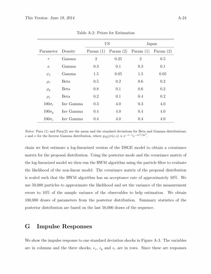
This Version: June 19, 2014 A-24
Table A-2: Priors for Estimation
US Japan
Parameter Density Param (1) Param (2) Param (1) Param (2)
τ Gamma 2 0.25 2 0.5
κ Gamma 0.3 0.1 0.3 0.1
ψ1 Gamma 1.5 0.05 1.5 0.05
ρr Beta 0.5 0.2 0.6 0.2
ρg Beta 0.8 0.1 0.6 0.2
ρz Beta 0.2 0.1 0.4 0.2
100σr Inv Gamma 0.3 4.0 0.3 4.0
100σg Inv Gamma 0.4 4.0 0.4 4.0
100σz Inv Gamma 0.4 4.0 0.4 4.0
Notes: Para (1) and Para(2) are the mean and the standard deviations for Beta and Gamma distributions;
s and ν for the Inverse Gamma distribution, where pIG(σ|ν, s) ∝ σ−ν−1e−νs2/2σ2
.
chain we first estimate a log-linearized version of the DSGE model to obtain a covariance
matrix for the proposal distribution. Using the posterior mode and the covariance matrix of
the log-linearized model we then run the RWM algorithm using the particle filter to evaluate
the likelihood of the non-linear model. The covariance matrix of the proposal distribution
is scaled such that the RWM algorithm has an acceptance rate of approximately 50%. We
use 50,000 particles to approximate the likelihood and set the variance of the measurement
errors to 10% of the sample variance of the observables to help estimation. We obtain
100,000 draws of parameters from the posterior distribution. Summary statistics of the
posterior distribution are based on the last 50,000 draws of the sequence.
G Impulse Responses
We show the impulse response to one standard deviation shocks in Figure A-3. The variables
are in columns and the three shocks, εz, εg and εr are in rows. Since these are responses

This Version: June 19, 2014 A-25
from a nonlinear model, we need to explain how we run the experiments. We start with
100 draws from the ergodic distribution for the U.S., conditioning on s = 0 and s = 1
separately. Then using these 100 draws as initial states along with their associated s value,
we compute the response of the economy to each shock relative to a baseline with no impulse.
In both economies all exogenous variables evolve according to their stochastic processes and
throughout the duration of the exercise the value of s remains the same. In the figure we
report the point-wise median response in percentage units.
Figure A-3: Impulse Responses - U.S. Ergodic Distribution
εz
Interest Rate (%)
5 10 15 200
0.1
0.2
0.3
0.4Inflation (%)
5 10 15 20−0.6
−0.4
−0.2
0
0.2Output (Level) (%)
5 10 15 200
0.2
0.4
0.6
0.8
εg
5 10 15 200
0.2
0.4
0.6
0.8
5 10 15 20−0.4
−0.2
0
0.2
0.4
5 10 15 200
0.1
0.2
0.3
0.4
εr
5 10 15 200
0.1
0.2
0.3
0.4
5 10 15 20−0.8
−0.6
−0.4
−0.2
0
5 10 15 20−0.2
−0.15
−0.1
−0.05
0
s=0s=1
The responses when s = 1 is entirely standard: a technology shock increases output
and interest rates and reduces inflation, a demand shock increases all there variables and
a monetary policy shock increases interest rates and reduces inflation and output. With

This Version: June 19, 2014 A-26
s = 0 a few significant differences emerge. First, the effect of shocks die out quicker. Second,
monetary policy shocks have a very muted effect on inflation and output. Third, and most
importantly, a positive government spending (demand) shock reduces inflation, as opposed
to increase it as in when s = 1. This is because the aggregate demand curve becomes upward
sloped when s = 0, similar to what Mertens and Ravn (2014) discuss.
H Particle Filter For Sunspot Equilibrium
The particle filter is used to extract information about the state variables of the model from
data on output growth, inflation, and nominal interest rates over the periods 1984:Q1 to
2013:Q4 (U.S.) and 1981:Q1 to 2013:Q4 (Japan).
H.1 State-Space Representation
Let dt be the 3× 1 vector of observables consisting of output growth, inflation, and nominal
interest rates. The vector xt stacks the continuous state variables, which are given by
xt = [Rt, yt, yt−1, zt, gt, At]′ and st ∈ {0, 1}, is the Markov-switching process.
dt = Ψ(xt) + νt (A.35)
P{st = 1} =
(1− p00) if st−1 = 0
p11 if st−1 = 1(A.36)
xt = Fst(xt−1, εt) (A.37)
The first equation is the measurement equation, where νt ∼ N(0,Σν) is a vector of mea-
surement errors. The second equation represents the law of motion of the Markov-switching
process. The third equation corresponds to the law of motion of the continuous state vari-
ables. The vector εt ∼ N(0, I) stacks the innovations εz,t, εg,t, and εR,t. The functions F0(·)
and F1(·) are generated by the model solution procedure. We subsequently use the densities
p(dt|xt), p(st|st−1), and p(xt|xt−1, st) to summarize the measurement and the state transition
equations.

This Version: June 19, 2014 A-27
H.2 Sequential Importance Sampling Approximation
Let wt = [x′t, st]′ and Dt0:t1 = {dt0 , . . . , dt1}. Particle filtering relies on sequential importance
sampling approximations. The distribution p(wt−1|D1:t−1) is approximated by a set of pairs
{(z(i)t−1, π(i)t−1)}Ni=1 in the sense that
1
N
N∑i=1
f(w(i)t−1)π
(i)t−1
a.s.−→ E[f(wt−1)|D1:t−1], (A.38)
where w(i)t−1 is the i’th particle, π
(i)t−1 is its weight, and N is the number of particles. An
important step in the filtering algorithm is to draw a new set of particles for period t. In
general, these particles are drawn from a distribution with a density that is proportional
to g(wt|D1:t, w(i)t−1), which may depend on the particle value in period t − 1 as well as the
observation dt in period t. This procedure leads to an importance sampling approximation
of the form:
E[f(wt)|D1:t] =
∫wt
f(wt)p(dt|wt)p(wt|D1:t−1)
p(dt|D1:t−1)dwt (A.39)
=
∫wt−1:t
f(wt)p(dt|wt)p(wt|wt−1)p(wt−1|D1:t−1)
p(dt|D1:t−1)dwt−1:t
≈1N
∑Ni=1 f(w
(i)t )
p(dt|w(i)t )p(w
(i)t |w
(i)t−1)
g(w(i)t |D1:t,w
(i)t−1)
π(i)t−1
1N
∑Nj=1
p(dt|w(j)t )p(w
(j)t |w
(j)t−1)
g(w(j)t |D1:T ,w
(i)t−1)
π(i)t−1
=1
N
N∑i=1
f(w(i)t )
(π(i)t
1N
∑Nj=1 π
(j)t
)=
1
N
N∑i=1
f(w(i)t )π
(i)t ,
where the unnormalized and normalized probability weights are given by
π(i)t =
p(dt|w(i)t )p(w
(i)t |w
(i)t−1)
g(w(i)t |D1:T , w
(i)t−1)
π(i)t−1 and π
(i)t =
π(i)t∑N
j=1 π(j)t
, (A.40)
respectively. In simple versions of the particle filter, w(i)t is often generated by simulating
the model forward, which means that g(w(i)t |D1:T , w
(i)t−1) ∝ p(w
(i)t |w
(i)t−1), and the formula for
the particle weights simplifies considerably. Unfortunately, this approach is quite inefficient
in our application, and we require a more elaborate density g(·|·) described below that
accounts for information in dt. The resulting extension of the particle filter is known as
auxiliary particle filter, e.g. Pitt and Shephard (1999).

This Version: June 19, 2014 A-28
H.3 Filtering
Initialization. To generate the initial set of particles {(w(i)0 , π
(i)0 }Ni=1, for each i, simulate
the DSGE model for T0 periods, starting from the targeted-inflation steady state, and set
π(i)0 = 1.
Sequential Importance Sampling. For t = 1 to T :
1. {w(i)t−1, π
(i)t−1}Ni=1 is the particle approximation of p(wt−1|D1:t−1). For i = 1 to N :
(a) Draw w(i)t conditional on w
(i)t−1 from g(wt|D1:t, w
(i)t−1).
(b) Compute the unnormalized particle weights π(i)t according to (A.40).
2. Compute the normalized particle weights π(i)t and the effective sample size ESSt =
N2/∑N
i=1(π(i)t )2.
3. Resample the particles via deterministic resampling (see Kitagawa (1996)). Reset
weights to be π(i)t = 1 and approximate p(wt|D1:t) by {(w(i)
t , π(i)t )}ni=1.
H.4 Tuning of the Filter
In the empirical analysis, we set T0 = 50 and N = 1, 000, 000. We also fix the measurement
error variance for output growth, inflation, and interest rates to be equal to 10% of the
sample variance of these series. We assume that the economies are in the targeted-inflation
regime during the initialization period. Since our model has discrete and continuous state
variables, we write
p(wt|wt−1) =
p0(xt|xt−1, st = 0)P{st = 0|st−1} if st = 0
p1(xt|xt−1, st = 1)P{st = 1|st−1} if st = 1
and consider proposal densities of the form
q(wt|wt−1, dt) =
q0(xt|xt−1, dt, st = 0)λ(wt−1, dt) if st = 0
q1(xt|xt−1, dt, st = 1)(1− λ(wt−1, dt)) if st = 1,
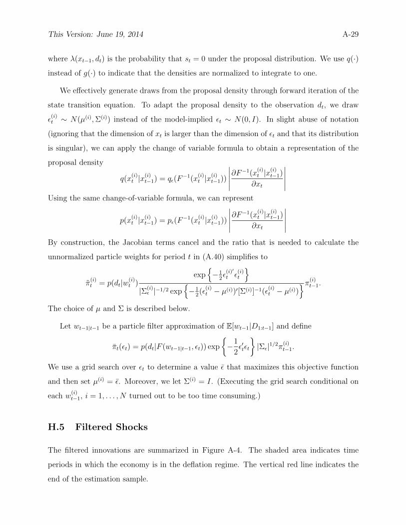
This Version: June 19, 2014 A-29
where λ(xt−1, dt) is the probability that st = 0 under the proposal distribution. We use q(·)
instead of g(·) to indicate that the densities are normalized to integrate to one.
We effectively generate draws from the proposal density through forward iteration of the
state transition equation. To adapt the proposal density to the observation dt, we draw
ε(i)t ∼ N(µ(i),Σ(i)) instead of the model-implied εt ∼ N(0, I). In slight abuse of notation
(ignoring that the dimension of xt is larger than the dimension of εt and that its distribution
is singular), we can apply the change of variable formula to obtain a representation of the
proposal density
q(x(i)t |x
(i)t−1) = qε(F
−1(x(i)t |x
(i)t−1))
∣∣∣∣∣∂F−1(x(i)t |x(i)t−1)∂xt
∣∣∣∣∣Using the same change-of-variable formula, we can represent
p(x(i)t |x
(i)t−1) = pε(F
−1(x(i)t |x
(i)t−1))
∣∣∣∣∣∂F−1(x(i)t |x(i)t−1)∂xt
∣∣∣∣∣By construction, the Jacobian terms cancel and the ratio that is needed to calculate the
unnormalized particle weights for period t in (A.40) simplifies to
π(i)t = p(dt|w(i)
t )exp
{−1
2ε(i)′
t ε(i)t
}|Σ(i)
ε |−1/2 exp{−1
2(ε
(i)t − µ(i))′[Σ(i)]−1(ε
(i)t − µ(i))
}π(i)t−1.
The choice of µ and Σ is described below.
Let wt−1|t−1 be a particle filter approximation of E[wt−1|D1:t−1] and define
πt(εt) = p(dt|F (wt−1|t−1, εt)) exp
{−1
2ε′tεt
}|Σε|1/2π(i)
t−1.
We use a grid search over εt to determine a value ε that maximizes this objective function
and then set µ(i) = ε. Moreover, we let Σ(i) = I. (Executing the grid search conditional on
each w(i)t−1, i = 1, . . . , N turned out to be too time consuming.)
H.5 Filtered Shocks
The filtered innovations are summarized in Figure A-4. The shaded area indicates time
periods in which the economy is in the deflation regime. The vertical red line indicates the
end of the estimation sample.

This Version: June 19, 2014 A-30
Figure A-4: Filtered Shocks
U.S. 1984-2013 Japan 1981-2013
εg
1985 1990 1995 2000 2005 2010−5
0
5
εz
1985 1990 1995 2000 2005 2010−5
0
5
εr
1985 1990 1995 2000 2005 2010−5
0
5
εg
1985 1990 1995 2000 2005 2010−5
0
5
εz
1985 1990 1995 2000 2005 2010−5
0
5
εr
1985 1990 1995 2000 2005 2010−5
0
5