Managerial Decision Making and Problem Solving

Lecture Notes 1

Introduction The body of knowledge involving

quantitative approaches to decision making is referred to as Management Science Operations Research Decision Science

What is Management Science? Management Science is the discipline that

adapts the scientific approach for problem solving to help managers make informed decisions.

The goal of management science is to recommend the course of action that is expected to yield the best outcome with what is available.

What is Management Science? The basic steps in the management science

problem solving process involves Analyzing business situations (problem definition); Building mathematical models to describe the

business situation(Mathematical Modeling); Solving the mathematical models; Communicating/implementing recommendations

based on the models and their solutions.

Problem Definition Steps to be taken

Observe operations Ease into complexity Recognize political realities Decide (identify) what is really wanted Identify constraints Seek continuous feedback

Mathematical Modeling This is a procedure that recognizes and

verbalizes a problem and then quantifies it using mathematical expressions.

Steps to be taken Identify decision variables Quantify the objective and constraints Construct a model shell Data gathering – consider time/cost issues

Classification of Mathematical Models

Classification by the model purpose Optimization models Prediction models

Classification by the degree of certainty of the data in the model Deterministic models Probabilistic (stochastic) models

Solving the Mathematical Model

Steps to be taken Choose an appropriate technique Generate model solution Test/ validate model results Return to modeling step if results are

unacceptable Perform “what-if” analysis

Communication / Implementation

Prepare a business report Be concise Use everyday language Make liberal use of graphics

Monitor the progress of the implementation

Communication / Implementation

Components of a business presentation Introduction Assumptions/approximations made Solution approach/ computer program used Results What-if analysis Overall recommendation Appendices

Management Science Applications

Linear Programming was used by Burger King to find how to best blend cuts of meat to minimize costs.

Integer Linear Programming model was used by American Air Lines to determine an optimal flight schedule.

The Shortest Route Algorithm was implemented by the Sony Corporation to developed an onboard car navigation system.

Management Science Applications

Project Scheduling Techniques were used by a contractor to rebuild Interstate 10 damaged in the 1994 earthquake in the Los Angeles area.

Decision Analysis approach was the basis for the development of a comprehensive framework for planning environmental policy in Finland.

Queuing models are incorporated into the overall design plans for Disneyland and Disney World, which lead to the development of ‘waiting line entertainment’ in order to improve customer satisfaction.

Introduction to Linear Programming

A Linear Programming model seeks to maximize or minimize a linear function, subject to a set of linear constraints.

The linear model consists of the followingcomponents: A set of decision variables. An objective function. A set of constraints.

Introduction to Linear Programming

A feasible solution satisfies all the problem's constraints.

An optimal solution is a feasible solution that results in the largest possible objective function value when maximizing (or smallest when minimizing).

A graphical solution method can be used to solve a linear program with two variables.

Introduction to Linear Programming

There are efficient solution techniques that solve linear programming models.

The output generated from linear programming packages provides useful “what if” analysis.

Introduction to Linear Programming The Importance of Linear Programming

Many real world problems lend themselves to linear programming modeling.

Many real world problems can be approximated by linear models.

There are well-known successful applications in: Manufacturing Marketing Finance (investment) Advertising Agriculture

Introduction to Linear Programming

Assumptions of the linear programming model The parameter values are known with certainty. The objective function and constraints exhibit

constant returns to scale. There are no interactions between the decision

variables. The Continuity assumption: Variables can take

on any value within a given feasible range.

Example 1

Max 5Max 5xx11 + 7 + 7xx22

s.t. s.t.

xx11 << 6 6

22xx11 + 3 + 3xx22 << 19 19

xx11 + + xx22 << 8 8

xx11 >> 0 and 0 and xx22 >> 0 0

19

The non-negativity constraints

X2

X1

Graphical Analysis – the Feasible Region

Example 1: Graphical Solution

xx11

xx22

88

77

66

55

44

33

22

11

1 1 2 2 3 3 4 4 5 5 6 6 7 7 8 8 9 109 10

22xx11 + 3 + 3xx22 = 19= 19

xx11 + + xx22 = 8 = 8

xx11 = 6 = 6

FeasibleFeasible RegionRegion

The search for an optimal solution

Start at some arbitrary value for objective function, then increase the value of the objective function, if possible, and continue until it becomes infeasible.

xx11

xx22

55xx11 + + 7x7x2 2 = 35= 3555xx11 + + 7x7x2 2 = 35= 35

88

77

66

55

44

33

22

11

1 1 2 2 3 3 4 4 5 5 6 6 7 7 8 8 9 109 10

55xx11 + + 7x7x2 2 = 42= 4255xx11 + + 7x7x2 2 = 42= 42

55xx11 + + 7x7x2 2 = 39= 3955xx11 + + 7x7x2 2 = 39= 39

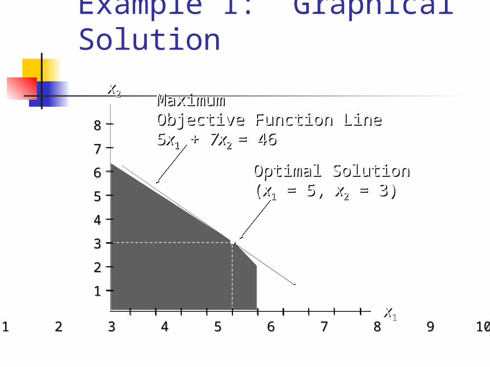
Example 1: Graphical Solution

xx11

xx22 MaximumMaximumObjective Function LineObjective Function Line55xx11 + + 7x7x2 2 = 46= 46

MaximumMaximumObjective Function LineObjective Function Line55xx11 + + 7x7x2 2 = 46= 46

Optimal SolutionOptimal Solution((xx11 = 5, = 5, xx22 = 3) = 3)Optimal SolutionOptimal Solution((xx11 = 5, = 5, xx22 = 3) = 3)

88

77

66

55

44

33

22

11

1 1 2 2 3 3 4 4 5 5 6 6 7 7 8 8 9 109 10

Extreme points and optimal solutions

There are three types of feasible points Interior points Boundary points Extreme points

If a linear programming problem has an optimal solution, an extreme point is optimal.

Example 1: Extreme Points

xx11

FeasibleFeasible RegionRegion

1111 2222

3333

4444

5555

xx22

88

77

66

55

44

33

22

11

1 1 2 2 3 3 4 4 5 5 6 6 7 7 8 8 9 109 10

(0, 6 (0, 6 ))

(5, 3)(5, 3)

(0, 0)(0, 0)

(6, 2)(6, 2)

(6, 0)(6, 0)

Multiple optimal solutions For multiple optimal solutions to exist, the

objective function must be parallel to one of the constraints.

The Role of Sensitivity Analysis of the Optimal Solution

Is the optimal solution sensitive to changes in input parameters?

Possible reasons for asking this question: Parameter values used were only best estimates. Dynamic environment may cause changes. “What-if” analysis may provide economical

and operational information.

Slack and Surplus Variables A linear program in which all the variables are non-

negative and all the constraints are equalities is said to be in standard form.

Standard form is attained by adding slack variables to "less than or equal to" constraints, and by subtracting surplus variables from "greater than or equal to" constraints.

Slack and surplus variables represent the difference between the left and right sides of the constraints.

Slack and surplus variables have objective function coefficients equal to 0.