Managing Warranties: Funding a Warranty Reserve and

Outsourcing Prioritized Warranty Repairs

byPeter S. Buczkowski

A dissertation submitted to the faculty of the University of North Carolina at ChapelHill in partial fulfillment of the requirements for the degree of Doctor of Philosophy inthe Department of Statistics and Operations Research.

Chapel Hill2004

Approved by

Advisor: Professor Vidyadhar G. Kulkarni

Reader: Dr. Suheil Nassar

Reader: Professor Jayashankar M. Swaminathan

Reader: Professor Eylem Tekin

Reader: Professor Jon W. Tolle

c© 2004Peter S. Buczkowski

ALL RIGHTS RESERVED

ii

ABSTRACT

Peter S. Buczkowski: MANAGING WARRANTIES: FUNDING A WARRANTY

RESERVE AND OUTSOURCING PRIORITIZED WARRANTY REPAIRS

(Under the direction of Professor Vidyadhar G. Kulkarni)

We consider two problems central to the managing of warranty costs by the manufacturer.

First, we consider funding an interest-bearing warranty reserve with contributions after

each sale. The problem for the manufacturer is to determine the initial level of the

reserve fund and the amount to be put in after each sale, so as to ensure that the

reserve fund covers all the warranty liabilities with a prespecified probability over a fixed

period of time. We assume a non-homogeneous Poisson sales process, random warranty

periods, and an exponential failure rate for items under warranty. We derive the mean

and variance of the reserve level as a function of time and provide a heuristic to aid the

manufacturer in its decision.

We also consider the problem of outsourcing warranty repairs to outside vendors

when items have priorities in service. The manufacturer has a contract with a fixed

number of repair vendors. The manufacturer pays a fixed fee for each repair done by

a vendor which is independent of the repair type and priority class but depends on the

vendor. There are a fixed number of items under warranty, and each item belongs to

one of a fixed number of priority classes. The manufacturer also pays for holding costs

incurred when the items are at the vendors, the holding cost being higher for the higher

priority items. The vendors provide a pre-emptive priority for an item over all other items

of lower priority. We focus on static allocation of the warranty repairs; that is, we assign

iii

all items to the vendors at the beginning of the warranty period. We give the known

algorithm to optimally solve the one priority class problem and solve the multi-priority

class problem by formulating it as a convex minimum cost network flow problem. Then,

we give numerical examples to illustrate the cost benefits of a multi-priority structure.

iv

ACKNOWLEDGMENTS

I am sincerely grateful to my advisor, Dr. Vidyadhar Kulkarni, for his knowledge,

guidance, time, and support through my studies at Chapel Hill. His comments greatly

improved this dissertation from beginning to end.

I would also like to express my gratitude to my committee members: Dr. Suheil

Nassar, Dr. Jayashankar M. Swaminathan, Dr. Eylem Tekin, and Dr. Jon W. Tolle, for

their help and suggestions on my research. Special thanks to Dr. Mark Hartmann for

donating his time and providing invaluable suggestions, without which this dissertation

would not be complete. Let me also extend thanks to my classmates, especially Wei

Huang, Bala Krishnamoorthy, Michelle Opp, and Rob Pratt. Their advice and support

is evident in many areas of this thesis.

Finally, I would like to thank my wife Gretchen for her support and understanding

over the last four years.

v

CONTENTS

LIST OF TABLES . . . . . . . . . . . . . . . . . . . . . . . . . . . . . . . . . . viii

LIST OF FIGURES . . . . . . . . . . . . . . . . . . . . . . . . . . . . . . . . . ix

1 Introduction 1

1.1 Overview . . . . . . . . . . . . . . . . . . . . . . . . . . . . . . . . . . . . 1

1.2 Literature Review . . . . . . . . . . . . . . . . . . . . . . . . . . . . . . . 2

1.3 Organization of the Dissertation . . . . . . . . . . . . . . . . . . . . . . . 6

2 Funding a Warranty Reserve 8

2.1 Overview . . . . . . . . . . . . . . . . . . . . . . . . . . . . . . . . . . . . 8

2.2 Notation and Assumptions . . . . . . . . . . . . . . . . . . . . . . . . . . 8

2.3 Probability Distribution of the Number of Items Under Warranty . . . . 11

2.3.1 Distribution of Xn(t) . . . . . . . . . . . . . . . . . . . . . . . . . 11

2.3.2 Distribution of Xo(t) . . . . . . . . . . . . . . . . . . . . . . . . . 12

2.4 Differential Equations for Moments of R(t) . . . . . . . . . . . . . . . . . 15

2.5 Solution for Moments of R(t) . . . . . . . . . . . . . . . . . . . . . . . . 24

2.5.1 Example: Constant Warranty Period and Constant Sales Rate . . 25

2.6 Deciding the Values of c and R0 . . . . . . . . . . . . . . . . . . . . . . . 28

2.6.1 Distribution of R(t) . . . . . . . . . . . . . . . . . . . . . . . . . . 28

2.6.2 Heuristic for Deciding c and R0 . . . . . . . . . . . . . . . . . . . 30

2.7 Numerical Computations . . . . . . . . . . . . . . . . . . . . . . . . . . . 33

vi

3 Warranty Reserve: Extensions 36

3.1 Random contribution to the reserve after each sale . . . . . . . . . . . . 36

3.2 Multiple products using a single reserve . . . . . . . . . . . . . . . . . . . 37

3.3 Xo(t) is known during [0, T ] . . . . . . . . . . . . . . . . . . . . . . . . . 38

4 Outsourcing Prioritized Warranty Repairs 42

4.1 Overview . . . . . . . . . . . . . . . . . . . . . . . . . . . . . . . . . . . . 42

4.2 Notation and Assumptions . . . . . . . . . . . . . . . . . . . . . . . . . . 43

4.3 Problem Formulation . . . . . . . . . . . . . . . . . . . . . . . . . . . . . 45

4.4 Single Priority Class . . . . . . . . . . . . . . . . . . . . . . . . . . . . . 48

4.5 Minimum Cost Network Flow Problems . . . . . . . . . . . . . . . . . . . 52

4.5.1 Convex Network Problems . . . . . . . . . . . . . . . . . . . . . . 55

4.6 Network Flow Formulation . . . . . . . . . . . . . . . . . . . . . . . . . . 57

4.6.1 Single Priority Class . . . . . . . . . . . . . . . . . . . . . . . . . 57

4.6.2 Two Priority Classes . . . . . . . . . . . . . . . . . . . . . . . . . 59

4.6.3 Multiple Priority Classes . . . . . . . . . . . . . . . . . . . . . . . 61

4.7 Computational Issues . . . . . . . . . . . . . . . . . . . . . . . . . . . . . 64

4.8 An Example . . . . . . . . . . . . . . . . . . . . . . . . . . . . . . . . . . 67

4.9 Cost Benefits of the Multi-Priority Approach . . . . . . . . . . . . . . . . 68

4.10 Selecting the Values of Ki . . . . . . . . . . . . . . . . . . . . . . . . . . 70

5 Conclusions and Future Work 74

Bibliography 77

vii

LIST OF TABLES

2.1 Suggested Values for q . . . . . . . . . . . . . . . . . . . . . . . . . . . . 32

2.2 Simulation Results . . . . . . . . . . . . . . . . . . . . . . . . . . . . . . 35

4.1 Arc Properties for Two-priority Network . . . . . . . . . . . . . . . . . . 59

4.2 Arc Properties for m-priority Network . . . . . . . . . . . . . . . . . . . 63

4.3 Costs and Service Rates for Each Vendor . . . . . . . . . . . . . . . . . . 68

4.4 Average Holding Costs for Vendors . . . . . . . . . . . . . . . . . . . . . 69

4.5 Vendor Properties for Similar Cost Example . . . . . . . . . . . . . . . . 70

4.6 Arc Properties for the Reward Network . . . . . . . . . . . . . . . . . . . 72

4.7 Costs and Service Rates for Each Vendor . . . . . . . . . . . . . . . . . . 73

viii

LIST OF FIGURES

2.1 Example of Warranty Reserve Account . . . . . . . . . . . . . . . . . . . 9

2.2 Examples of Confidence Bands for R(t) . . . . . . . . . . . . . . . . . . . 29

2.3 Expected Reserve for Various Values of X(0) . . . . . . . . . . . . . . . . 34

4.1 Network Model of Single Priority Problem . . . . . . . . . . . . . . . . . 57

4.2 Network Model of Two-priority Problem . . . . . . . . . . . . . . . . . . 59

4.3 Network Model of m Priority Problem . . . . . . . . . . . . . . . . . . . 62

4.4 Network Model of Reward Problem . . . . . . . . . . . . . . . . . . . . . 72

ix

Chapter 1

Introduction

1.1 Overview

Since the Magnuson-Moss Warranty Act of 1975 [33], manufacturers are required to

provide a warranty for all consumer goods which cost more than $15. Warranties play

an important role in the consumer-manufacturer relationship. They offer assurance to

the consumer that their purchase will achieve certain performance standards through at

least the warranty period. The manufacturers use warranties as a marketing tool and

they limit their liability.

When designing product warranties, the manufacturers must decide on many is-

sues, such as warranty policy, length of warranty period, repair policy, and quality control.

They also have to plan to cover the costs associated with the warranty. An issue of criti-

cal importance to the manufacturers is managing the costs associated with the warranty

effectively. Our research investigates two key questions of planning for these costs.

The first is of funding a warranty reserve account with contributions made after

each sale. A warranty reserve is used to accommodate all of the costs associated with the

servicing of a warranty of a product. We model a policy that is currently implemented in

industry; that of adding a fraction of each sale to the reserve fund. There are a variety

1

of goals that a manufacturer may have regarding its warranty reserve. Two general goals

are to keep the reserve above some target dollar amount B > 0 and to not have an

excessive amount of money in the reserve. The reasoning behind these goals is simple:

a shortage requires extra administrative costs and may even have legal ramifications,

while an excessive surplus locks money in the reserve that may be more useful for other

business interests. Achieving these goals requires careful planning.

We also consider the problem of outsourcing warranty repairs to outside vendors

when items have priority levels. For example, some warranty contracts specify the repair

turnaround time (e.g. 1 day, 3 days, or 7 days). With careful management, repair out-

sourcing can be a major benefit to the manufacturer. A smooth operation can improve

customer satisfaction and turnaround times, while allowing the manufacturer to main-

tain its focus on production. While the manufacturer may have a central repair depot,

it often is not effective to ship items to the depot due to time and cost constraints. Thus

it might be beneficial to choose repair vendors distributed geographically so as to be

close to the customers. The manufacturer must seek a balance between cost savings and

customer service. If not, some customers will be lost because of poor service. Repair

outsourcing is an especially important problem when considering priorities because high

priority customers will typically inflict greater loss if the manufacturer does not meet

their expectations.

1.2 Literature Review

Warranty theory has been heavily studied over the past two decades. Blischke and

Murthy [5] wrote a comprehensive reference for the subject. They discuss many differ-

ent types of warranty policies, including many warranty policies currently implemented

in industry. Numerous cost and optimization models are developed from both the con-

sumer’s and the manufacturer’s point of view, including life cycle and long-run average

2

cost models. We use these models to compute the expected warranty cost of a product

in our numerical examples.

Many of the early papers on warranty theory discuss the costs and other effects

that are associated with warranties. Glickman and Berger [13] consider the effect of

warranty on demand by assuming that demand increases as the warranty period increases.

Warranty costs affect both the buyer and the seller. Mamer [23] wrote the first

paper to provide a comprehensive model of both the buyer’s and seller’s expected costs

and long-run average costs for the free replacement warranty. Our research focuses on

the manufacturers’ view of warranty costs.

The concept of a warranty reserve is a topic of many research works. The initial

papers on warranty reserves discussed here consider a fixed product lot size throughout

the life cycle of a product (or equivalently, a fixed cumulative failure rate). Menke [25]

wrote one of the first papers to address the warranty reserve problem. He concentrates

on calculating the expected warranty cost over a given warranty period for two types

of pro-rata warranty policies (linear rebate and lump-sum rebate) assuming a constant

product failure rate. Amato and Anderson [2] extend Menke’s model by allowing the

reserve fund to accrue interest, requiring the consideration of discounted costs. A com-

parison to Menke’s results is made, concluding that discounting significantly reduces the

expected warranty reserve over longer periods of time. Both models are rather limited in

scope because they only consider pro-rata warranty policies and an exponential failure

distribution.

Balcer and Sahin [4] derive the moments of the total replacement cost for both

the free-replacement and pro-rata warranty policies during the product life cycle. They

assume that successive failure times form a renewal process.

Mamer [24] uses renewal theory to model repeated product failures over a life cycle

of the product. He incorporates discounting in his model and allows for a general failure

distribution. However, he does not consider the sales process nor compute a reserve.

3

Tapiero and Posner [32] allow for a portion of each sale to be set aside for future

warranty costs. The contributions to the reserve fund and the items sold occur at a

constant rate. The claims are generated according to a compound Poisson Process and

they use a sample path technique to compute the long-run probability distribution of the

warranty reserve.

Eliashberg, Singpurwalla, and Wilson [12] calculate the reserve for a product

whose failure rate is indexed by two scales, time and usage. They allow for a general

failure rate and assume a form of imperfect repair. The warranty reserve is computed to

minimize a loss function for the manufacturer.

Ja, et al. [18] compute the distribution of the total discounted warranty cost over

the life cycle of the product. They analyze the discounted warranty cost of a single sale

under many different policies and then consider different stochastic sales processes. A

single contribution to the reserve is made at the beginning of the life cycle. However, the

subtractions from the reserve due to warranty costs are tracked as a function of time.

Another application related to the warranty reserve problem is the insurance pre-

mium problem. An insurance company must decide on the monthly premium to charge

a certain class of customer. Low premiums result in loss to the insurer, while high pre-

miums result in loss of business to the competition. A discussion of this can be found

in [30]. There are other related problems, including the funding of a company’s pension

plan. Many of these problems are solved using actuarial models, particularly collective

risk (loss) models (see [22] and [9] for references on this subject). However, the current

models do not incorporate the number of policies insured by the company at any given

time.

The works described above illustrate many different models to compute the war-

ranty reserve. However, they assume that the reserve is either funded at the beginning

of the product sales period or at a constant rate. We extend this research by modeling

4

contributions to the reserve after each sale and allowing the cumulative warranty claim

rate to depend on the sales process.

We now turn to the warranty repair outsourcing problem. At its most basic struc-

ture, the static allocation model reduces to a resource allocation problem with integer

variables. Without considering priorities, the problem has a separable objective function.

This problem has been widely studied in the literature. Gross [15] first proposed a simple

greedy algorithm to find the optimal solution if the objective is convex.

Several authors have since expanded the problem. Ibarki and Katoh [16] pro-

vide a comprehensive review of resource allocation problems and algorithms to solve

them. Their bibliography provides a review of the literature up to 1988. Bretthauer and

Shetty [6], [7] also give a survey of a generalization: the nonlinear knapsack problem.

They provide a proof of the greedy algorithm by the generalized Lagrange multiplier

method. Zaporozhets [34] gives an alternate proof of the greedy algorithm. Opp, et al.

[28] describes the greedy algorithm in detail for the convex separable resource alloca-

tion problem and its application to our problem without priorities. Also discussed are

some computational issues associated with the application, mostly regarding the expected

queue length.

Once priorities are considered, the objective is no longer separable. We extend the

previous research by providing an algorithm to optimally solve the closed static allocation

problem with priorities. We have developed a new proof of the greedy algorithm when

there is only one priority class, and give a new algorithm to handle the special structure of

the objective when there are multiple priority classes. Finally, we investigate the benefits

of a multi-priority structure for the manufacturer.

5

1.3 Organization of the Dissertation

In Chapter 2, we address the problem of funding a warranty reserve. In the first two

sections, we provide an overview of the problem and the notations and assumptions used

throughout Chapters 2 and 3. In Section 2.3, we derive the probability distribution for

the number of items under warranty at time t. We follow that with differential equations

for the first and second moment of the reserve level in Section 2.4. The general solutions

to these equations are provided in the following section along with the special case of

a constant warranty period. We provide a heuristic for determining the values of the

contribution amount after each sale and the initial reserve level in Section 2.6 and some

simulation results in Section 2.7.

We consider three extensions of the warranty reserve problem in Chapter 3:

• The reserve contribution after the jth sale is a random variable. (Section 3.1)

• The manufacturer maintains a single reserve fund for multiple products or multiple

warranties. (Section 3.2)

• The remaining lifetimes of the items sold prior to time t are known. (Section 3.3)

Next, we turn to the warranty repair outsourcing problem in Chapter 4. After

a brief problem overview, we state the notation and assumptions of the problem in

Section 4.2. In Section 4.3, we derive the cost function and state the optimization problem

for the model. We provide the known algorithm to solve the single priority problem in

Section 4.4 and give a new proof of the algorithm. Our algorithm to solve the m-priority

problem uses network concepts. We give a brief overview of minimum cost network flow

problems in Section 4.5. Then we reformulate the optimization problem as a convex

minimum cost flow problem and provide the algorithm to solve the problem. We provide

the simplified algorithm for the one- and two-priority case and give the general algorithm

for the m-priority case. In Section 4.7, we discuss the computational issues that arise in

6

the problem and provide an example in the following section. In Section 4.9, we illustrate

the cost benefits of the priority structure. We provide two examples: the first with very

different holding costs between the high and low priority customers and the second with

relatively similar holding costs between the high and low class customers. We complete

the discussion of the outsourcing problem in Section 4.10 by presenting an optimization

problem for the manufacturer when the customer pays additional monies for priority in

service.

7

Chapter 2

Funding a Warranty Reserve

2.1 Overview

In this chapter, we consider the problem of funding a warranty reserve account. We

consider a manufacturer who adjusts its warranty reserve at a series of fixed time points

(e.g. at times 0, T, 2T, . . .). In this dissertation, we consider a single period [0, T ]. The

manufacturer must decide on the initial amount in the reserve at the beginning of the

period and the contribution amount from each sale. We derive the mean and variance of

the reserve level as a function of time and provide a heuristic to aid the manufacturer in

its decision.

2.2 Notation and Assumptions

We begin by introducing some notation and assumptions. We define R(t) as the amount

in the reserve at time t, where t = 0 represents the beginning of the period. The reserve

fund accrues interest at constant rate α > 0. At each sale, an amount c is contributed

to the account. The manufacturer must decide on the initial reserve level, R0, and the

contribution amount to the reserve from each sale, c, at the beginning of the period.

Let S(t) be the total number of sales up to time t. We assume that {S(t), t ≥ 0} is

8

a nonhomogeneous Poisson Process with a known rate function θ(·) (we call this an

NPP (θ(·))). Each item is under warranty for a random amount of time. The warranty

durations are independent and identically distributed with common cdf F (·) and mean w.

Also, the warranty durations are independent of any future failures. Note that this allows

for a constant warranty period. The customer always makes a warranty claim at each

product failure. We assume instantaneous repair and that the repair times of a given

item follow a Poisson Process with rate λ. The repair cost of the ith failure (at time Yi)

is Di, a random variable. The Di’s are i.i.d. and are independent of the failure time. Let

D(t) be the total undiscounted cost of all claims up to time t; hence

D(t) =∑

i:Yi≤t

Di.

Let X(t) denote the number of items under warranty at time t and Sj denote the

time of the jth sale. The manufacturer observes the number of items under warranty at

time 0 to aid in his determination of R0 and c. The manufacturer may or may not know

the remaining warranty lifetimes of the items under warranty at time 0; we consider both

cases. Figure 2.1 illustrates the evolution of the warranty reserve over time.

YS 2 2

1D

D2

D3

dollars

0

S

c

c

time31 1Y Y

R

Figure 2.1: Example of Warranty Reserve Account

9

For computational purposes, it is helpful to distinguish between the effects of the

items sold since time 0 from the items sold before time 0. We will break X(t) into two

parts: let Xn(t) represent the number of items under warranty at time t that were sold

after time 0, and let Xo(t) represent the number of items under warranty at time t that

were sold prior to time 0. We write

R(t) = Rn(t) +Ro(t),

where Rn(t) is the portion of the reserve related to the new items Xn(t), and Ro(t) is the

portion of the reserve related to the old items Xo(t). Thus, in Rn(t), we add contributions

from new purchases and only subtract the claims generated by new items. In Ro(t), there

are no new contributions, so we only subtract claims generated by old items. Similarly,

we define Dn(t) (Do(t)) as the total undiscounted claims from time 0 to t generated

by the new (old) items. It is convenient to define Rn(0) = 0 and Ro(0) = R0. In our

model we track both Rn(t) and Ro(t) for ease in computation, while the manufacturer

just tracks R(t).

We will calculate first and second moments for some of the functions R(t), S(t),

X(t), D(t) and their components (Rn(t), Ro(t), etc.). We represent this by using lower

case for the first moment and using lower case with a subscript of 2 for the second moment

(e.g. r(t) = E[R(t)] and r2(t) = E[R2(t)]). Any exception to this will be mentioned at

the appropriate place throughout the thesis. Also, we will use ∆h to indicate the change

in a function from t to t + h. For example, ∆hR(t) = R(t + h) − R(t). Finally, we will

use the standard o(h) notation for a function g(h) when

limh→0

g(h)

h= 0.

10

2.3 Probability Distribution of the Number of Items

Under Warranty

In this section we derive the distributions for Xn(t) and Xo(t).

2.3.1 Distribution of Xn(t)

First we explore the {Xn(t), t ≥ 0} process. At time t, items are purchased according to

an NPP (θ(·))). The amount of time an item is under warranty is a random variable with

cdf F (·). We assume there is no capacity on the total number of items under warranty

at any time. Therefore, we can model the {Xn(t), t ≥ 0} process as an Mt/G/∞ queue

with arrival rate θ(·) and service time distribution F (·).

The following result was established independently by Palm [29] and Khintchine

[21]. Most recently, Eick, Massey, and Whitt [11] provided a simpler proof of this result

and developed some further results for the Mt/G/∞ queue.

Theorem 1 Let Q(t) be the number of items in an Mt/G/∞ queue at time t with arrival

rate θ(·) and i.i.d. service times S with cdf F (·). At time t, there are 0 items in the queue.

Then, for each time point t ≥ 0, Q(t) has a Poisson distribution with mean

E

t∫

t−S

θ(u)du

=

t∫

0

θ (t− u) [1 − F (u)] du.

Therefore, the moments of Xn(t) are

xn(t) =

t∫

0

θ (t− u) [1 − F (u)] du, and (2.1)

xn2 (t) = xn(t) + (xn(t))2 . (2.2)

11

2.3.2 Distribution of Xo(t)

We consider two possible cases for the items sold prior to time 0: either the manufacturer

fully knows the remaining warranty durations of all items under warranty at time 0 or that

the remaining warranty durations are i.i.d. random variables with common cdf Q(t). The

former case is rather easy to handle – the entire sample path of X o(t) is a deterministic

function. If the remaining warranty durations are unknown, the probability that the

remaining warranty duration of an item is greater than t, given that it was under warranty

at time 0, is 1 −Q(t). Hence,

Xo(t) ∼ Bin (X(0), 1 −Q(t)) ,

where X(0) is the number of items under warranty at time 0. The moments are

xo(t) = X(0)(1 −Q(t)), and (2.3)

xo2(t) = X(0)Q(t) (1 −Q(t)) + (xo(t))2 . (2.4)

One choice for Q(t) is obtained from the stationary distribution of the remaining

service times in an M/G/∞ queue in steady state. From Takacs [31], we have the

following lemma.

Lemma 1 (Takacs, Theorem 3.2.2) : Let X(t) be the number of items under war-

ranty at time t, and let Li(t) denote the remaining warranty period of item i under

warranty. The sales process is a Poisson process. If w <∞, we have

limt→∞

P (Li(t) < xi ∀ i = 1, . . . , k |X(t) = k) =k∏

i=1

1

w

xi∫

0

[1 − F (s)] ds,

and the limiting distribution is independent of the initial state.

12

Therefore, under the assumption of Poisson input in steady state, we have that

the remaining warranty distributions are independent of each other and the probability

that an item is still under warranty at time t, given that it was under warranty at time 0

is

1 −Q(t) =1

w

∞∫

t

[1 − F (s)] ds, (2.5)

where Q(t) is determined by Lemma 1, i.e.

Q(t) =1

w

t∫

0

[1 − F (s)] ds. (2.6)

This result can be extended to the case of a non-homogeneous Poisson Process,

as shown in the following lemma.

Lemma 2 Let X(t) be the number of items under warranty at time t, and let Li(t)

denote the remaining warranty period of item i under warranty. Suppose that the sales

process begins at time −A, and {S(t), t ≥ −A} is a non-homogeneous Poisson with rate

function θ(·). We have

P (Li(t) < xi ∀ i = 1, . . . , k |X(t) = k) =

k∏

i=1

t+A∫

0

[F (s+ xi) − F (s)] θ(t− s)ds

t+A∫

0

[1 − F (s)] θ(t− s)ds

.

Proof. Since the sales process is an NPP (θ(·)), we know that for t ≥ −A,

P (X(t) = k) = exp

−

t+A∫

u=0

(1 − F (u))θ(t− u)du

(

t+A∫

s=0

(1 − F (s))θ(t− s)ds

)k

k!. (2.7)

13

We compute P (Li(t) < xi ∀ i = 1, . . . , k;X(t) = k). Let Θ(u) =u∫

s=−A

θ(s)ds. We have

P (Li(t) < xi∀ i = 1, . . . , k;X(t) = k)

=∞∑

n=k

e−Θ(t) Θ(t)n

n!

(

n

k

)

1

Θ(t)

t+A∫

0

F (s)θ(t− s)ds

n−k

·

k∏

i=1

1

Θ(t)

t+A∫

0

[F (xi + u) − F (u)]θ(t− u)du

= e−Θ(t) Θ(t)k

k!

∞∑

n=k

1

(n− k)!

t+A∫

0

F (s)θ(t− s)ds

n−k

·k∏

i=1

1

Θ(t)

t+A∫

0

[F (xi + u) − F (u)]θ(t− u)du

=e−Θ(t)

k!exp

t+A∫

0

F (s)θ(t− s)ds

k∏

i=1

t+A∫

0

[F (xi + u) − F (u)]θ(t− u)du

= exp

−

t+A∫

0

(1 − F (s))θ(t− s)ds

1

k!

k∏

i=1

t+A∫

0

[F (xi + u) − F (u)]θ(t− u)du. (2.8)

The conditional probability P (Li(t) < xi ∀ i = 1, . . . , k |X(t) = k) is Equation 2.8 di-

vided by Equation 2.7. We get

k∏

i=1

t+A∫

0

[F (xi + u) − F (u)]θ(t− u)du

t+A∫

0

(1 − F (s))θ(t− s)ds

.

This completes the proof.

The above lemma implies that for an NPP (θ(·)) sales process, we can use the

following for Q(t):

Q(t) =

∞∫

0

(F (t+ u) − F (u)) θ(−u)du

∞∫

0

(1 − F (s)) θ(−s)ds

. (2.9)

14

It is easy to check that Equation 2.9 reduces to Equation 2.6 if θ(t) = θ for all values of

t.

In the next section, we will need the moments of X(t), Xn(t), and Xo(t) in the

computation of the moments of R(t). Since Xn(t) and Xo(t) are independent of each

other, we compute the moments of X(t) as:

x(t) = xn(t) + xo(t), and (2.10)

x2(t) = xn2 (t) + xo

2(t) + 2xn(t)xo(t). (2.11)

2.4 Differential Equations for Moments of R(t)

We will consider two cases: Xo(t) is unknown during [0, T ] (here we use the distribution

discussed in Section 2.3.2), and Xo(t) is known in its entirety during [0, T ]. We cover

the former case here and the latter case in Section 3.3. In the results that follow, we will

need expressions for E[∆hS(t)] and E[∆hD(t)], where h is small. Since {S(t), t ≥ 0} is

an NPP (θ(·)), we know that

E[∆hS(t)] = E

t+h∫

u=t

θ(u)du

= θ(t)h+ o(h).

The stochastic process {D(t), t ≥ 0} is a random sum of random variables. Let N(t)

represent the number of claims from time 0 to t. For a given sample path of {X(t), t ≥ 0},

{N(t), t ≥ 0} is an NPP (λX(·)). The repair costs are i.i.d. with common mean E[D]

and second moment E[D2]. Therefore,

E[∆hD(t)] = E[∆hN(t)]E[D] = E

t+h∫

u=t

λX(u)du

E[D]

= λE[X(t)h]E[D] + o(h) = λx(t)E[D]h + o(h).

15

Similarly,

Var (∆hD(t)) = E[∆hN(t)]Var(D) + E2[D]Var(∆hN(t))

= λx(t)h[

E[D2] − E2[D]]

+ λx(t)E2[D]h+ o(h)

= λx(t)E[D2]h+ o(h).

We next introduce notation for item failure rates. Consider an arbitrary item that

was sold in [0, t]. Let U be its time of sale. Then, U has cdf

P (U ≤ u) =Θ(u)

Θ(t), 0 ≤ u ≤ t,

where Θ(t) =

t∫

0

θ(s)ds.

Let W represent the warranty period random variable. Then, the probability that the

item is under warranty at time t is P (U + W > t). Given that it is under warranty at

time t, the probability that its warranty expires in [t, t + δ] is given by

hn(t)δ =fU+W (t)

1 − FU+W (t)δ + o(δ). (2.12)

Since the warranty periods are i.i.d. and the sales process is an NPP , we see that the

items behave independently of each other. Hence, if Xn(t) = i, the probability that a

single items fails in [t, t + δ] is ihn(t)δ + o(δ). We do a similar analysis for the items

under warranty at time 0. We assume that the remaining lifetimes are unknown but are

independent of each other. The probability that an item is still under warranty at time

t is 1 −Q(t). The probability that its warranty expires in [t, t+ δ] is given by

ho(t)δ =−Q′(t)

1 −Q(t)δ + o(δ). (2.13)

16

For convenience, we define

H i(t) =

t∫

s=0

hi(s)ds, for i = n, o.

We are now ready to compute the moments of R(t).

Theorem 2 Let r(t) = E[R(t)]. Then,

dr(t)

dt= αr(t) + cθ(t) − λE[D]x(t), (2.14)

with initial condition r(0) = R0.

Proof. We look at the change in the reserve from time t to time t+ h, where h is small.

We have

R(t+ h) − R(t) = (eαh − 1)R(t) + c [∆hS(t)] − [∆hD(t)] + o(h).

Taking expectation on both sides, we get

r(t+ h) − r(t) = (eαh − 1)r(t) + c (E[∆hS(t)]) − (E[∆hD(t)]) + o(h),

= (αh+ o(h))r(t) + c(θ(t)h+ o(h)) − (λE[D]x(t)h + o(h))

Diving by h and taking the limit as h→ 0 yields Equation 2.14.

Deriving the differential equations for E[Rn(t)] and E[Ro(t)] is similar to Theo-

rem 2.

Theorem 3 Let rn(t) = E[Rn(t)] and ro(t) = E[Ro(t)]. Then,

drn(t)

dt= αrn(t) + cθ(t) − λE[D]xn(t),

dro(t)

dt= αro(t) − λE[D]xo(t),

17

with initial conditions rn(0) = 0 and ro(0) = R0.

Proof. The definitions of Rn(t) and Ro(t) in Section 2.2 yield:

Rn(t + h) −Rn(t) = (eαh − 1)Rn(t) + c[∆hS(t)] − ∆hDn(t) + o(h),

Ro(t+ h) − Ro(t) = (eαh − 1)Ro(t) − ∆hDo(t) + o(h).

The c term does not appear in the equation for Ro(t + h) since the revenue for sales is

only generated by the new items. We apply the same techniques used in Theorem 1 to

complete the result.

To derive the differential equation for the second moment, we first prove two

lemmas.

Lemma 3 Let v(t) = E[Ro(t)Xo(t)]. Then

dv(t)

dt= (α− ho(t)) v(t) − λE[D]xo

2(t), (2.15)

with initial condition v(0) = X(0)R0, and ho(t) is as in Equation 2.13.

Proof. We again look at v(t+ h) − v(t) and take limits as h→ 0.

v(t+ h) = E[Ro(t + h)Xo(t+ h)]

= E[(

eαhRo(t) − ∆hDo(t))

(Xo(t) + ∆hXo(t)) + o(h)],

v(t+ h) − v(t) = eαhE[Ro(t)∆hXo(t)] + (eαh − 1)E[Ro(t)Xo(t)] − E[∆hD

o(t)∆hXo(t)]−

E[∆hDo(t)Xo(t)] + o(h),

v(t+ h) − v(t) = (1 + αh+ o(h))E[Ro(t)∆hXo(t)] + (αh+ o(h)) v(t)−

E[∆hDo(t)∆hX

o(t)] − E[∆hDo(t)Xo(t)] + o(h). (2.16)

18

We can find E[Ro(t)∆hXo(t)], E[∆hD

o(t)Xo(t)], and E[∆hDo(t)∆hX

o(t)] by condition-

ing on Xo(t).

E[Ro(t)∆hXo(t)] =

∑

i

E[Ro(t)∆hXo(t)|Xo(t) = i]P [Xo(t) = i]

=∑

i

E[Ro(t)|Xo(t) = i]E[∆hXo(t)|Xo(t) = i]P [Xo(t) = i]

=∑

i

−E[Ro(t)|Xo(t) = i]iho(t)P [Xo(t) = i]h + o(h)

= −ho(t)∑

i

E[Ro(t)i|Xo(t) = i]P [Xo(t) = i]h+ o(h)

= −ho(t)v(t)h+ o(h).

E[∆hDo(t)Xo(t)] =

∑

i

E[∆hDo(t)Xo(t)|Xo(t) = i]P [Xo(t) = i]

=∑

i

iE[∆hDo(t)|Xo(t) = i]P [Xo(t) = i]

=∑

i

i2λP [Xo(t) = i]E[D]h+ o(h)

= λE[D]xo2(t)h + o(h).

E[∆hDo(t)∆hX

o(t)] =∑

i

E[∆hDo(t)∆hX

o(t)|Xo(t) = i]P [Xo(t) = i]

=∑

i

E[∆hDo(t)|Xo(t) = i]E[∆hX

o(t)|Xo(t) = i]P [Xo(t) = i]

=∑

i

−iλiho(t)E[D]P [Xo(t) = i]h2 + o(h)

= −λE[D]xo2(t)h

o(t)h2 + o(h) = o(h).

Plugging these three expressions into Equation 2.16, dividing by h, and taking the limit

as h→ 0 completes the result.

19

Lemma 4 Let u(t) = E[R(t)X(t)]. Then

du(t)

dt=(α− hn(t))u(t) + cθ(t) (x(t) + 1) − λE[D]x2(t) + θ(t)r(t)+

(hn(t) − ho(t)) ∗ (rn(t)xo(t) + v(t)) , (2.17)

with initial condition u(0) = X(0)R0, and where v(t) satisfies Lemma 3, hn(t) satisfies

Equation 2.12, ho(t) satisfies Equation 2.13, and rn(t) satisfies Theorem 3.

Proof. We proceed as in Lemma 3. We have

u(t+ h) = E [R(t+ h)X(t+ h)]

= E[(

eαhR(t) + c∆hS(t) − ∆hD(t))

(X(t) + ∆hX(t)) + o(h)]

,

u(t+ h) − u(t) = E[(eαh − 1)R(t)X(t)] + cE[∆hS(t)X(t)] − E[∆hD(t)X(t)]+

E[eαhR(t)∆hX(t)] + cE[∆hS(t)∆hX(t)] − E[∆hD(t)∆hX(t)] + o(h).

(2.18)

We investigate each term on the right hand side of Equation 2.18 below:

(1) E[(eαh − 1)R(t)X(t)] = (αh+ o(h))u(t).

(2) cE[∆hS(t)X(t)] = cE[∆hS(t)]E[X(t)] = cθ(t)x(t)h+o(h) (The number of additional

sales from t to t+ h is independent of the number of items under warranty at time t).

(3) We calculate E[∆hD(t)X(t)] by conditioning on X(t):∑

k

E[∆hD(t)X(t)|X(t) = k]P [X(t) = k] =∑

k

kE[∆hD(t)|X(t) = k]P [X(t) = k]

=∑

k

λk2P [X(t) = k]E[D]h+ o(h) = λE[D]x2(t)h+ o(h).

(4) E[R(t)∆hX(t)] = E[R(t)∆hXo(t)] + E[R(t)∆hX

n(t)].

We calculate E[R(t)∆hXo(t)] by conditioning on Xo(t):

E[R(t)∆hXo(t)] =

∑

i

E[R(t)∆hXo(t)|Xo(t) = i]P [Xo(t) = i]

20

=∑

i

E[R(t)|Xo(t) = i]E[∆hXo(t)|Xo(t) = i]P [Xo(t) = i]

=∑

i

−iho(t)E[R(t)|Xo(t) = i]P [Xo(t) = i]h+ o(h)

= −ho(t)∑

i

E[R(t)i|Xo(t) = i]P [Xo(t) = i]h + o(h)

= −ho(t)E[R(t)Xo(t)]h+ o(h)

= −ho(t)E [(Rn(t) +Ro(t))Xo(t)] h+ o(h)

= −ho(t) (E[Rn(t)Xo(t)] + E[Ro(t)Xo(t)]) h+ o(h)

= −ho(t) (rn(t)xo(t) + v(t)) h+ o(h).

We calculate E[R(t)∆hXn(t)] by conditioning on Xn(t):

E[R(t)∆hXn(t)] =

∑

i

E[R(t)∆hXn(t)|Xn(t) = i]P [Xn(t) = i]

=∑

i

E[R(t)|Xn(t) = i]E[∆hXn(t)|Xn(t) = i]P [Xn(t) = i]

=∑

i

E[R(t)|Xn(t) = i] (θ(t)h− ihn(t)h)P [Xn(t) = i] + o(h)

= θ(t)h∑

i

E[R(t)|Xn(t) = i]P [Xn(t) = i]

− hn(t)h∑

i

E[R(t)i|Xn(t) = i]P [Xn(t) = i] + o(h)

= θ(t)r(t)h− hn(t)E[R(t)Xn(t)]h + o(h)

= θ(t)r(t)h− hn(t) (E[R(t)X(t)] − E[R(t)Xo(t)]) h+ o(h)

= θ(t)r(t)h− hn(t) (u(t) − rn(t)xo(t) − v(t)) h+ o(h)

= θ(t)r(t)h− hn(t)u(t)h+ hn(t) (rn(t)xo(t) + v(t)) h+ o(h).

(5) To calculate E[∆hS(t)∆hX(t)], we must consider the dependence of S(t) and X(t). If

there is a sale in ∆ht, then both ∆hS(t) and ∆hX(t) are 1. This happens with probability

θ(t)h+ o(h). If there is an expiration, then ∆hX(t) is −1 while ∆hS(t) is 0 (hence their

21

product is 0). Therefore,

cE[∆hS(t)∆hX(t)] = cθ(t)h + o(h).

(6) We calculate E[∆hD(t)∆hX(t)] by conditioning on ∆hX(t):

∑

k

E[∆hD(t)∆hX(t)|∆hX(t) = k]P [∆hX(t) = k]

=∑

k

kE[∆hD(t)|∆hX(t) = k]P [∆hX(t) = k]

=∑

k

λk2E[D]

2P [∆hX(t) = k]h + o(h)

=λE[D]

2h(θ2(t)h2 + θ(t)h) + o(h) = o(h).

To complete the proof, we substitute the expressions found in (1)-(6) into Equation 2.18,

divide by h, and take the limit as h→ 0.

We are now ready to provide the differential equation for the second moment of

R(t).

Theorem 4 Let r2(t) = E[R2(t)] and r(t), u(t), v(t), and rn(t) be defined as before. Then

dr2(t)

dt= 2αr2(t) + c2θ(t) + λE[D2]x(t) + 2cθ(t)r(t) − 2λE[D]u(t), (2.19)

where r2(0) = R20.

Proof. We proceed as in Lemma 3. We have

R(t + h) = eαhR(t) + c∆hS(t) − ∆hD(t) + o(h).

Squaring both sides and rearranging terms, we get

R2(t + h) − R2(t) = (e2αh − 1)R2(t) + c2(∆hS(t))2 + (∆hD(t))2 + 2ceαhR(t)∆hS(t)−

22

2eαhR(t)∆hD(t) − 2c∆hS(t)∆hD(t) + o(h).

Taking expectation, we obtain

r2(t + h) − r2(t) = (e2αh − 1)r2(t) + c2E[∆hS(t)]2 + E[∆hD(t)]2 + 2ceαhE[R(t)∆hS(t)]−

2eαhE[R(t)∆hD(t)] − 2cE[∆hS(t)∆hD(t)] + o(h). (2.20)

We investigate each term of the right hand side of Equation 2.20 below:

(1) (e2αh − 1)r2(t) = (2αh+ o(h))r2(t).

(2) c2E[∆hS(t)]2 = c2 (θ(t)h + θ2(t)h2) + o(h) = c2θ(t)h + o(h).

(3) The mean and variance of ∆hD(t) was computed prior to Lemma 1. We have

E[∆hD(t)]2 = V ar(∆hD(t)) + E2[∆hD(t)]

= λE[D2]x(t)h+ (λE[D]x(t)h)2 + o(h)

= λE[D2]x(t)h+ o(h).

(4) R(t) is independent of ∆hS(t) since future sales do not impact the current reserve

level. Therefore, E[R(t)∆hS(t)] = E[R(t)]E[∆hS(t)] = θ(t)r(t)h + o(h).

(5) We calculate E[R(t)∆hD(t)] by conditioning on X(t):

∑

k

E[R(t)∆hD(t)|X(t) = k]P [X(t) = k]

=∑

k

E[R(t)|X(t) = k]E[∆hD(t)|X(t) = k]P [X(t) = k]

=∑

k

E[R(t)|X(t) = k]λkP [X(t) = k]E[D]h + o(h)

= λE[R(t)X(t)]E[D]h+ o(h) = λE[D]u(t)h+ o(h).

23

(6) We calculate E[∆hS(t)∆hD(t)] by conditioning on X(t):

=∑

k

E[∆hS(t)∆hD(t)|X(t) = k]P [X(t) = k]

=∑

k

E[∆hS(t)|X(t) = k]E[∆hD(t)|X(t) = k]P [X(t) = k]

=∑

k

θ(t)h ∗ λE[D]kP [X(t) = k]h+ o(h)

= θ(t)λE[D]x(t)h2 + o(h) = o(h).

To complete the proof, we substitute the expressions found in (1)-(6) into Equation 2.20,

divide by h, and take the limit as h→ 0.

Theorem 4 provides a system of equations for the first and second moments of

R(t). We can solve this linear system analytically by solving the equations in the following

order: r(t), ra(t), v(t), u(t), r2(t). This is because each differential equation only uses

functions of t that are either known or previously solved in the system – this is known as

a triangular system. We can also use a software package, such as MATLAB, to solve the

system numerically. Clearly, we can use the solution of the system to find the variance

by applying the formula

V ar(R(t)) = r2(t) − r2(t).

In the next section, we present the general solution to this system and some examples

for simple warranty distributions.

2.5 Solution for Moments of R(t)

We now provide the solution to the differential equations derived in Section 2.4. For a

complete solution, it is necessary to know the functions x(t), x2(t), xn(t), xo(t), ho(t),

hn(t), Ho(t), and Hn(t). These expressions, defined in Equations 2.1 – 2.13 of Section 2.3,

depend only on the warranty distribution F (·) and the given sales rate θ(·).

24

Theorem 5 Let r(t), rn(t), v(t), u(t), and r2(t) be defined as in Section 2.4. Then, we

have

r(t) = R0eαt + eαt

t∫

s=0

e−αs (cθ(s) − λE[D]x(s)) ds, (2.21)

rn(t) = eαt

t∫

s=0

e−αs (cθ(s) − λE[D]xn(s)) ds,

v(t) = X(0)R0eαt−Ho(t) − λeαt−Ho(t)E[D]

t∫

s=0

xo2(s)e

−αs+Ho(s)ds,

u(t) = X(0)R0eαt−Hn(t) + eαt−Hn(t)

t∫

s=0

e−αs+Hn(s)[(hn(s) − ho(s)) (rn(s)xo(s) + v(s))

+ cθ(s)(x(s) + 1) − λx2(s)E[D] + θ(s)r(s)] ds,

r2(t) = R20e

2αt + e2αt

t∫

s=0

e−2αs[

c2θ(s) + λx2(s)E[D2] + 2cθ(s)r(s) − 2λE[D]u(s)]

ds.

Proof. We apply the techniques to solve linear differential equations for each of r(t),

rn(t), v(t), u(t), and r2(t). For the sake of brevity, we omit the details.

2.5.1 Example: Constant Warranty Period and Constant Sales

Rate

We provide the solution for the first and second moments of R(t) for the example of a

constant warranty period w and a constant sales rate function θ(t) = θ for all t ≥ 0. The

second moment r2(t) is quite complex, so we instead provide the variance of R(t).

First, we provide the moments of Xn(t) and Xo(t), and the expressions for F (t),

hn(t), and ho(t). We assume that the remaining warranty periods of the items sold

prior to time 0 is unknown. We apply the result from Section 2.3.2 to determine the

distribution of Xn(t). We have

25

F (t) =

0, 0 ≤ t < w

1, t ≥ w, and

t∫

0

θ (t− u) [1 − F (u)] du = θmin(t, w).

Applying the formulas for the first and second moments of Xn(t) and Xo(t) yields

xn(t) = θmin(t, w),

xn2 (t) = θmin(t, w) + θ2 min(t2, w2),

xo(t) =

X(0)(

w−tw

)

0 ≤ t < w

0 t ≥ w,

xo2(t) =

X(0)(

(w−t)tw2

)

+(

X(0)(

w−tw

))20 ≤ t < w

0 t ≥ w.

Using the expressions for hn(t) and ho(t) defined in 2.12 and 2.13, we obtain

hn(t) =

0, t < w

1w

t ≥ w, and

ho(t) =

1w−t

, t < w

0 t ≥ w.

We consider two cases.

Case 1. 0 ≤ t ≤ w. Here, we have

r(t) = A0 + A1t+ A2eαt, and

V ar(R(t)) = C0 + C1t + C2t2 + C3e

αt + C4teαt + C5e

2αt,

26

where

A0 =1

α2

(

λE[D]θ + λE[D]X(0)α− cθα−λE[D]X(0)

w

)

,

A1 =λE[D]

αw(θw −X(0)) ,

A2 = −1

α2

(

λE[D]θ + λE[D]X(0)α−λE[D]X(0)

w− cθα− R0α

2

)

,

C0 =1

4α4w2

(

6λ2θE2[D]αw2 − 4λ2X(0)E2[D] − 4λcθE[D]α2w2 + 6λ2X(0)E2[D]αw

−λθE[D2]α2w2 + λX(0)E[D2]α2w − 2λX(0)E[D2]α3w2 − 2c2θα3w2)

,

C1 =1

2α3w2

(

λX(0)E[D2]α2w − 4λ2X(0)E2[D] + 2λ2θE2[D]αw2

+2λ2X(0)E2[D]αw − λθE[D2]α2w2)

,

C2 = −λ2X(0)E2[D]

α2w2,

C3 =2E[D]

α4w2

(

λcθα2w2 + λ2X(0)E[D] − λ2θE[D]αw2 − λ2X(0)E[D]αw)

,

C4 =2λ2X(0)E2[D]

α3w2, and

C5 =1

4α4w2

(

λθE[D2]α2w2 + 2c2θα3w2 + 2λX(0)E[D2]α3w2 + 2λ2θE2[D]αw2

−λX(0)E[D2]α2w − 4λ2X(0)E2[D] + 2λ2X(0)E2[D]αw − 4λcθE[D]α2w2)

.

Case 2. t > w. In this case, there are no longer any old items under warranty. Therefore,

we have

r(t) = A0 + A1(t− w) + A2eα(t−w) + r(w), and

V ar(R(t)) = C0 + C1(t− w) + C2eα(t−w) + C3e

2α(t−w) + V ar(R(w)),

where

A0 =θ

α2(λE[D] − cα) ,

A1 =θλE[D]α

α2,

27

A2 =1

α2

(

cθα +R0α2 − λθE[D]

)

,

C0 =1

4α3

(

6λ2θE2[D] − 4λcθE[D]α− 2c2θα2 − λθE[D2]α)

,

C1 =1

2α2

(

2λ2θE2[D] − λθE[D2]α)

,

C2 =2

α3

(

λcθE[D]α− λ2θE2[D])

, and

C3 =1

4α3

(

λθE[D2]α + 2c2θα2 − 4λcθE[D]α + 2λ2E[D2]θ)

.

2.6 Deciding the Values of c and R0

The manufacturer must decide on the values of c and R0 at the beginning of a new

period, with the goal of satisfying all of the warranty costs in the period while remaining

above some target B > 0 with some prespecified probability 1 − β. Of course, setting

artificially high values of c and R0 will achieve this goal, but this will tie up excess money

that may be used for other business interests. In this section, we suggest criteria that

the manufacturer may use as a basis for its decision.

2.6.1 Distribution of R(t)

We first point out that the variance of R(t) is independent of the initial reserve level, R0.

Let Si be the time of the ith sale, and let Yj be the time of the jth failure (with repair

cost Di). Then, the reserve at time t can be computed as:

R(t) = R0eαt + c

∑

Si≤t

eα(t−Si) −∑

Yi≤t

Dieα(t−Yi). (2.22)

Note that the last 2 terms of Equation 2.22 are the random components of R(t) and do

not contain R0. Therefore, the variance is independent of R0 and only depends on the

variable c; we use this fact in deriving a heuristic to determine the values of c and R0 in

the next section.

28

In general, the distribution of R(t) is difficult to determine. However, if the sales

process is a non-homogeneous Poisson Process, the distribution is asymptotic Normal as

the number of sales becomes large. A proof of this can be obtained as a minor extension

of the result given by Ja [17], which is based on [18]. Therefore, we use the Normal

distribution as an approximation. In our simulations, the values of R(t) seem to follow

a Normal distribution, especially for large t. We show an example in the next section.

Let Φ(·) be the standard Normal cumulative distribution function (zero mean

and variance one) and let zβ be the number such that Φ (zβ) = 1 − β. Therefore, at a

given point of t, approximately 100(1 − β)% of sample paths of R(t) will remain above

r(t) − zβ

√

V ar(R(t)). The two examples in Figure 2.2 show examples of sample paths

of R(t) and the 100(1 − 2β)% confidence bands at each value of t. In each graph, the

jagged line represents a typical sample path of R(t). The smooth central line is the plot

of r(t), while the outer lines are the plots of r(t) ± zβ

√

V ar(R(t)). In the left graph,

mint∈[0,T ]

r(t)−zβ

√

V ar(R(t)) occurs at time T , while the minimum in the right graph occurs

within (0, T ).

0 0.1 0.2 0.3 0.4 0.55000

5500

6000

6500

7000

7500

8000

8500

time

r(t)

0 0.1 0.2 0.3 0.4 0.55000

5500

6000

6500

7000

7500

8000

8500

9000

9500

10000

time

r(t)

Figure 2.2: Examples of Confidence Bands for R(t)

29

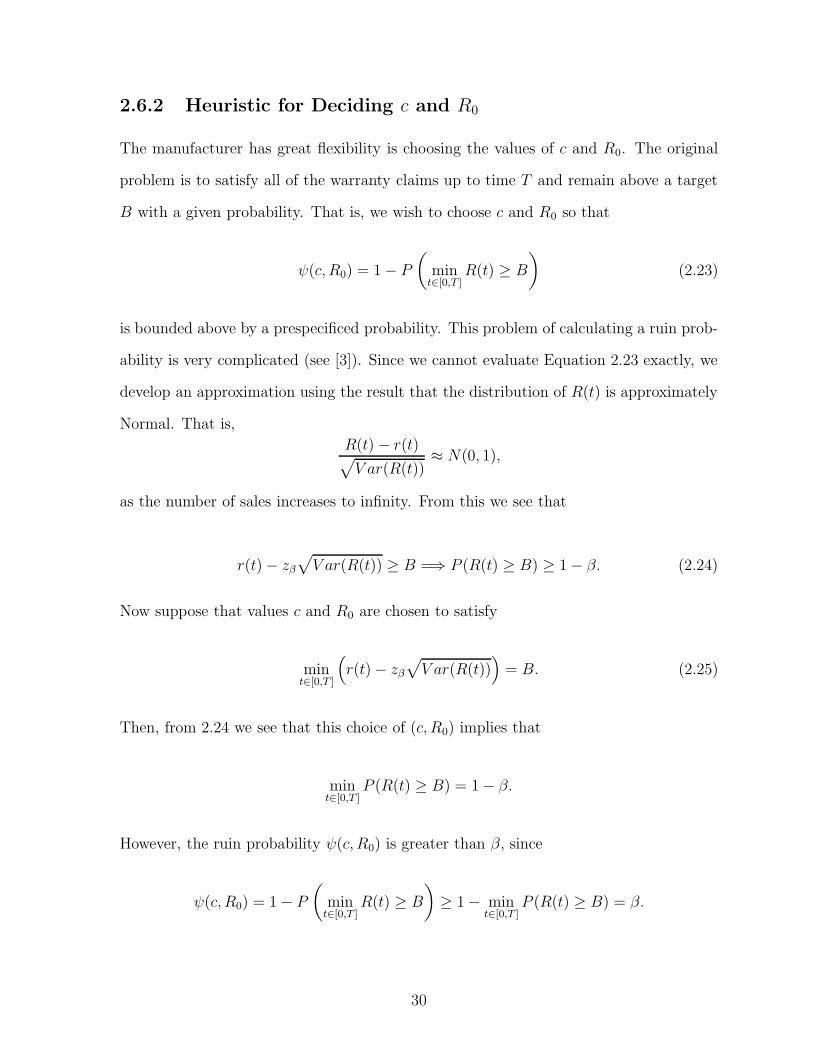
2.6.2 Heuristic for Deciding c and R0

The manufacturer has great flexibility is choosing the values of c and R0. The original

problem is to satisfy all of the warranty claims up to time T and remain above a target

B with a given probability. That is, we wish to choose c and R0 so that

ψ(c, R0) = 1 − P

(

mint∈[0,T ]

R(t) ≥ B

)

(2.23)

is bounded above by a prespecificed probability. This problem of calculating a ruin prob-

ability is very complicated (see [3]). Since we cannot evaluate Equation 2.23 exactly, we

develop an approximation using the result that the distribution of R(t) is approximately

Normal. That is,

R(t) − r(t)√

V ar(R(t))≈ N(0, 1),

as the number of sales increases to infinity. From this we see that

r(t) − zβ

√

V ar(R(t)) ≥ B =⇒ P (R(t) ≥ B) ≥ 1 − β. (2.24)

Now suppose that values c and R0 are chosen to satisfy

mint∈[0,T ]

(

r(t) − zβ

√

V ar(R(t)))

= B. (2.25)

Then, from 2.24 we see that this choice of (c, R0) implies that

mint∈[0,T ]

P (R(t) ≥ B) = 1 − β.

However, the ruin probability ψ(c, R0) is greater than β, since

ψ(c, R0) = 1 − P

(

mint∈[0,T ]

R(t) ≥ B

)

≥ 1 − mint∈[0,T ]

P (R(t) ≥ B) = β.

30

Thus β provides a lower bound on the ruin probability ψ(c, R0). Intuitively, the quantities

β and ψ(c, R0) appear to be related. We use simulation to help uncover a possible

relationship between the two quantities.

Therefore, we estimate a parameter qβ so that

mint∈[0,T ]

(

r(t) − qβ√

V ar(R(t)))

= B (2.26)

=⇒ P

(

mint∈[0,T ]

R(t) > B

)

≈ 1 − β.

Clearly we cannot guarantee that such a qβ will work in all possible situations, but we

believe such an estimate will be instructive to a manufacturer.

Since there are many values of c and R0 which will satisfy Equation 2.25, we offer

a heuristic to select one set. The heuristic assumes that we have an additional condition

to satisfy: at time T , the expected reserve level is R0eαT (to account for accumulated

interest). Therefore, we choose c so that

r(T ) = R0eαT .

From Equation 2.21, we see that this is equivalent to solving the equation

eαT

T∫

s=0

e−αs (cθ(s) − λE[D]x(s)) ds = 0. (2.27)

This equation does not contain R0. Rearranging Equation 2.27 to isolate the variable c

yields

c =

λE[D]T∫

s=0

e−αsx(s)ds

T∫

s=0

e−αsθ(s)ds

. (2.28)

31

We use this value of c in solving Equation 2.25. Since the left hand side of Equation 2.25

is a monotone increasing function of R0, there is a unique value of R0 that satisfies the

equation.

We used simulation to estimate qβ for different values of β. For ten different sets

of parameter values and distributions, we ran 5000 trials and recorded the minimum

value of R(t) (and the occurence time t∗) over [0, T ] for each trial. We first recorded

the time, tB, when r(t) − zβ

√

V ar(R(t)) reached its minimum value over [0, T ] for the

given parameters. Then, for each simulated trial, we record the minimum value of the

reserve level R(t∗) and the time of occurence t∗. We select q so that the simulated reserve

process R(t) lies above r(t) − q√

V ar(R(t)) for all t ∈ [0, T ]. The quantity q is given by

the following formula:

q =r(tB) − R(t∗)√

V ar(R(tB)).

We then computed the 100(1 − β)th percentile of q for each parameter set i (call this

qiβ). Our suggested value of qβ for each value of β is maxiqiβ. In our experience, the

worst cases (large qiβ) occurred when the minimum of r(t)−zβ

√

V ar(R(t)) did not occur

at time T . However, the dispersion in qiβ for the different parameter sets was not large

enough to consider different cases. For reference, we give the values of zβ to compare

with our suggested values of qβ. We also give the range and standard deviation of qiβ to

note the relative error in the estimate. The results are summarized in Table 2.1.

β zβ qβ maxiqiβ − min

iqiβ

√

V ar(qiβ)

.10 1.282 1.842 0.441 0.146

.05 1.645 2.197 0.414 0.152.025 1.960 2.594 0.501 0.168.01 2.326 3.059 0.492 0.174.005 2.576 3.349 0.591 0.205.001 3.090 4.163 0.814 0.275

Table 2.1: Suggested Values for q

32

The values for qiβ in each of the simulation trials are not vastly different from zβ.

For β > .01, the value of max qiβ − min qiβ was less than 0.5 and the standard deviation

of qiβ was less than 0.2. From our experience, the value of qiβ is most affected by the

variation in the repair costs and the initial number of items under warranty. While these

estimates for qβ will not work for all problems, we observed that they were fairly robust

for our simulations. We applied the heuristic with these values of qβ for other parameter

sets and always had {R(t) > B ∀ t} in at least 100(1 − β)% of the trials.

This heuristic has many advantages: it is easy to compute, provides stability to

the expected reserve level from period to period, yields a unique answer, and performs

well under simulation.

2.7 Numerical Computations

We dedicate this section to a numerical example. Consider a non-renewable, free-

replacement warranty with constant period 1 year. All the items are independent and

identical, with mean 0.1 failures per year and each replacement cost to the manufacturer

is fixed at $100. The sales process is a Poisson process with mean 1000/year. The in-

terest rate on the account is 6% compounded continuously, and we consider a period T

of one-half year. Some products that might have this structure are electronic devices

(such as calculators) or small appliances (such as toasters or microwaves). More complex

products, such as computers, have similar properties where repairs are ”good as new”.

Let E[CW (α)] be the expected total warranty cost discounted to present value

for a single item. One option for the manufacturer is to contribute this amount to the

reserve after each sale. We compute E[CW (α)] by the following formula (see Section 4.2

of [5]):

E[CW (α)] = E[D]

W∫

0

eαtdM(t), (2.29)

33

where M(·) is the ordinary renewal function associated with the product failure distribu-

tion (here M(t) = λt). Substituting the numbers of the example yields E[CW (α)] = 9.71.

We use this as a comparison for the recommended value of c obtained through the heuris-

tic.

First, we illustrate the effect of X(0) on the mean of the reserve. Figure 2.3

plots r(t) for X(0) = {500, 1000, 1500, 2000}. Note that the expected number of items

under warranty in steady state is given by θw = 1000. In each case, we set the reserve

contribution from each sale to E[CW (α)] = 9.71.

0 0.05 0.1 0.15 0.2 0.25 0.3 0.35 0.4 0.45 0.52000

3000

4000

5000

6000

7000

8000

9000

time

r(t)

X(0)=500

X(0)=1000

X(0)=1500

X(0)=2000

Figure 2.3: Expected Reserve for Various Values of X(0)

This plot clearly shows that letting c = E[CW (α)] is very effective if X(0) ≈ θw.

However, if these two values are far apart, another value of c is recommended. In the

instance when X(0) = 2000, it requires a value of c = 17.51 to keep the expected reserve

level at the end of the period equal to R0eαT . Conversely, a value of c = 6.24 achieves

the same goal when X(0) = 500.

Next, we illustrate the heuristic to determine c and R0 when there are 1500 items

under warranty at time 0 and the remaining warranty periods of these items are unknown.

34

Suppose that the manufacturer must keep the reserve level above B = 5000 for the entire

period [0, T ] with 95% probability. Plugging the parameters into Equation 2.28, we get

c = 13.756. We see from Table 2.1 that q.05 = 2.197. We solve Equation 2.26 for R0,

obtaining a value of R0 = 6734.8.

We ran 5000 simulated trials with the above parameters to illustrate the effective-

ness of the heuristic and check for normality of R(t). For reference this set of parameters

is different from the 10 used to determine q. Of the 5000 trials, 223 (4.46%) of them

fell below the target B = 5000 at some point during the period [0, T ]. This is slightly

less than the target of 5%. We recorded the values of R(t) of each trial at time points

t = 0.125, 0.25, 0.375, and 0.5. We compare the average and standard deviation of the

simulated trials with the theoretical values calculated in Section 2.5. Also, we give the

p-value of the chi-squared test for a Normal distribution. We summarize the results in

Table 2.2.

Time t0.125 0.25 0.375 0.5

Sim. 6658.2 6662.9 6757.9 6928.9Mean

Theor. 6668.6 6680.3 6770.5 6939.8Standard Sim. 453.5 641.8 775.9 886.7Deviation Theor. 454.8 636.7 772.1 882.9p-value of χ2-test 1.24·10−7 0.137 0.259 0.720

Table 2.2: Simulation Results

As expected, the simulated mean and standard deviation at each time point match

up with the theoretical mean and variance. Clearly, the p-value of the χ2-test increases

with increasing t. Although normality is clearly violated at t = 0.125, it is accepted at

t ≥ 0.25. Since the distribution is asymptotic Normal with respect to increasing sales,

we can be fairly confident that a large sales process will have an approximately Normal

distribution. Our example has a modest sales rate of 1000/yr; we see more intensive sales

processes lead to a Normal distribution much quicker.

35

Chapter 3

Warranty Reserve: Extensions

In this chapter we consider three separate extensions to our basic warranty reserve model:

• The reserve contribution after the jth sale is Cj, a random variable. (Section 3.1)

• There are multiple products for the manufacturer which use the same reserve fund.

For each product i, the sales rate is θi(·), the warranty period has cdf Fi(·), and

the reserve contribution after each sale of product i is a constant ci. (Section 3.2)

• The entire sample path of Xo(t) is known during [0, T ]. This case arises if the

manufacturer has access to the time of sale and the length of the warranty period

of each item under warranty. (Section 3.3)

3.1 Random contribution to the reserve after each

sale

Suppose that the contribution to the reserve after the ith sale is a random variable. We

assume that the successive contributions {Ci, i ≥ 1} are i.i.d and independent of the

reserve level and the sales process. A possible reason for having a random contribution

amount independent of the other relevant stochastic processes is when the product costs

36

a different amount in different distribution areas of the manufacturer. This assumption

is more critical in application areas such as insurance models or pension funds. We

can compute the moments of R(t) under this new assumption as in Section 2.4. Not

surprisingly, the only effect on the system of differential equations is a change from c to

E[C] and from c2 to E[C2].

Theorem 6 Let the reserve contributions after each sale be i.i.d random variables with

common mean E[C] and second moment E[C2]. Suppose they are independent of the

reserve level and the sales process. Then,

dr(t)

dt= αr(t) + E[C]θ(t) − λE[D]x(t),

drn(t)

dt= αrn(t) + E[C]θ(t) − λE[D]xn(t),

dv(t)

dt= (α− ho(t)) v(t) − λE[D]xo

2(t),

du(t)

dt= (α− hn(t)) u(t) + E[C]θ(t) (x(t) + 1) − λE[D]x2(t) + θ(t)r(t)

+ (hn(t) − ho(t)) ∗ (rn(t)xo(t) + v(t)) ,

dr2(t)

dt= 2αr2(t) + E[C2]θ(t) + λE[D2]x(t) + 2E[C]θ(t)r(t) − 2λE[D]u(t).

Proof. We recalculate each term in the derivations of the equations where the term c

originally occurred. We use the assumption that the contribution is independent of the

reserve level and the sales process to write E[CiM(t)] = E[C]E[M(t)] and E[C2i M(t)] =

E[C2]E[M(t)], where M(t) is a stochastic process independent of Ci. This occurs twice

in the derivations of dr(t)dt

, drn(t)dt

, and du(t)dt

, and three times in dr2(t)dt

.

3.2 Multiple products using a single reserve

Suppose that a manufacturer manages warranties for k products which may be k different

products, the same product with k different warranty policies, or a combination of the

37

two. It may be desirable for the manufacturer to have a single warranty reserve for

all of these products. We can apply our previous results to handle this situation. For

each product i, we assume that the sales process is an NPP (θi(·)), the failure rate is

exponential with rate λi, the contribution to the reserve after each sale is ci, and each

of these are independent of the other products. We track the total reserve contribution

from each of the products and denote this as Ri(t). The mean and variance of Ri(t) is

computed from the results in section 2.4.

Since each of the products are independent of each other, the total expected

reserve E[R(t)] can be computed as a sum of the independent expected reserves of each

product and the total variance V ar(R(t)) is the sum of the individual variances of each

product:

E[R(t)] = E

[

k∑

i=1

Ri(t)

]

=k∑

i=1

E[Ri(t)],

√

V ar(R(t)) =

√

√

√

√

k∑

i=1

V ar(Ri(t)).

It is clearly beneficial to maintain a combined account rather than k separate

ones, due to pooling of the risks involved. Mathematically, this is because the variances

combine additively, so the standard deviation of the combined reserve is less than the

sum of the standard deviation of k individual reserves.

3.3 Xo(t) is known during [0, T ]

The case where Xo(t) is known is much easier than when it is unknown. We still divide

X(t) as

X(t) = Xo(t) +Xn(t),

with the change that Xo(t) is a deterministic quantity.

38

Theorem 7 Let r(t) = E[R(t)], rn(t) = E[Rn(t)], y(t) = E[Rn(t)Xn(t)], and r2(t) =

E[R2(t)]. Assume that {Xo(t), 0 ≤ t ≤ T} is known. Then

dr(t)

dt= αr(t) + cθ(t) − λE[D]x(t),

drn(t)

dt= αrn(t) + cθ(t) − λE[D]xn(t),

dy(t)

dt= (α− hn(t)) y(t) + cθ(t) (1 + xn(t)) + θ(t)rn(t) − λE[D]xn

2 (t), (3.1)

dr2(t)

dt= 2αr2(t) + c2θ(t) + λE[D2]x(t) + 2cθ(t)r(t)

− 2λE[D] [Xo(t)r(t) + ro(t)xn(t) + y(t)] , (3.2)

where r(0) = R0, rn(0) = 0, u(0) = 0, and r2(0) = R2

0.

Proof. We apply the same proof technique as in Section 2.4. Most of the calculations

are exactly the same; we will mention and omit these and just provide the changes.

The calculations for dr(t)dt

and drn(t)dt

are the same as in Theorems 2 and 3. Since

dy(t)dt

is a new quantity, we provide the calculations.

y(t+ h) = E [Rn(t+ h)Xn(t+ h)]

= E[(

eαhRn(t) + c∆hS(t) − ∆hD(t))

(Xn(t) + ∆hXn(t)) + o(h)

]

y(t+ h) − y(t) = E[(eαh − 1)Rn(t)Xn(t)] + cE[∆hS(t)Xn(t)] − E[∆hDn(t)Xn(t)]+

E[eαhRn(t)∆hXn(t)] + cE[∆hS(t)∆hX

n(t)] − E[∆hDn(t)∆hX

n(t)] + o(h)

(3.3)

We investigate each term on the right hand side of Equation 3.3. The expressions for

E[(eαh − 1)Rn(t)Xn(t)], cE[∆hS(t)Xn(t)], E[∆hS(t)∆hXn(t)], and E[∆hD

n(t)∆hXn(t)]

are computed very similarly to their counterparts from Lemma 4. The computations

yield

E[(eαh − 1)Rn(t)Xn(t)] = (αh+ o(h))y(t),

39

cE[∆hS(t)Xn(t)] = cθ(t)xn(t)h+ o(h),

E[∆hS(t)∆hXn(t)] = cθ(t)h + o(h), and

E[∆hDn(t)∆hX

n(t)] = o(h)

We compute the other two quantities below:

(1) We calculate E[∆hDn(t)Xn(t)] by conditioning on Xn(t):

∑

k

E[∆hDn(t)Xn(t)|Xn(t) = k]P [Xn(t) = k] =

∑

k

kE[∆hDn(t)|Xn(t) = k]P [Xn(t) = k]

=∑

k

λk2P [Xn(t) = k]E[D]h + o(h) = λE[D]xn2 (t)h + o(h).

(2) We calculate E[Rn(t)∆hXn(t)] by conditioning on Xn(t):

E[Rn(t)∆hXn(t)] =

∑

i

E[Rn(t)∆hXn(t)|Xn(t) = i]P [Xn(t) = i]

=∑

i

E[Rn(t)|Xn(t) = i]E[∆hXn(t)|Xn(t) = i]P [Xn(t) = i]

= θ(t)rn(t)h−∑

i

ihn(t)E[Rn(t)|Xn(t) = i]P [Xn(t) = i] + o(h)

= θ(t)rn(t)h− hn(t)E[Rn(t)Xn(t)]h + o(h)

= θ(t)rn(t)h− hn(t)y(t)h+ o(h).

To obtain Equation 3.1, we substitute the expressions found in (1)-(6) into Equation 3.3,

divide by h, and take the limit as h→ 0.

It remains to derive Equation 3.2. We proceed in the usual fashion, beginning with

Equation 2.20 derived in Section 2.4. The only change from the derivation in Theorem

4 is in E[R(t)∆hD(t)]; we provide that below:

E[R(t)∆hD(t)] =∑

k

E[R(t)∆hD(t)|X(t) = k]P [X(t) = k]

=∑

k

E[R(t)|X(t) = k]E[∆hD(t)|X(t) = k]P [X(t) = k]

40

=∑

k

E[R(t)|X(t) = k]λkP [X(t) = k]E[D]h + o(h)

= λE[R(t)X(t)]E[D]h+ o(h)

= λE[D] [Xo(t)r(t) + ro(t)xn(t) + E[Rn(t)Xn(t)]] + o(h)

= λE[D] [Xo(t)r(t) + ro(t)xn(t) + y(t)]]h + o(h).

Making this substitution, we obtain Equation 3.2, completing the proof.

A manufacturer might use both assumptions regarding Xo(t). For example, if

they obtain a new computer package that tracks every customer’s warranty expiration

date during [0, T ], they may use the original assumption in the period [0, T ] but use their

additional information in the period [T, 2T ]. We leave as future work the case where the

purchase times of the items sold before time 0 are known, but the remaining warranty

periods are not.

41

Chapter 4

Outsourcing Prioritized Warranty

Repairs

4.1 Overview

We now discuss the problem of outsourcing warranty repairs when items have priority

in service. Consider a manufacturer that has a contract with V repair vendors for a

fixed fee per repair. Specifically, vendor j charges the manufacturer cj dollars for each

repair made under warranty, independent of the type of repair and the priority of the

item. The contract does not specify a minimum or maximum number of repairs. Usually

this contract situation arises when the manufacturer provides the replacement parts and

the vendor just executes the repairs. Another scenario is that the vendor charges the

expected cost per repair over the duration of the contract. We only consider a closed

population model, i.e., we assume the number of items under warranty at any given time

is constant.

For most manufacturers, it is important to return some repaired items faster than

others. One example is a company that makes large purchases with the manufacturer.

They will expect a faster repair turnaround time than an individual customer. Occasion-

42

ally, the manufacturer will include a maximum repair turnaround time in the purchase

contracts with a large purchaser. Also, the manufacturer might offer a choice of war-

ranties that specify the repair turnaround time. For example, the standard product

warranty guarantees a one week repair turnaround time but can be upgraded by the

customer to a two day repair turnaround time. The length of these turnaround times

require that some of the repairs take priority over others. We treat the case where each

item belongs to one of m priority classes.

The manufacturer must assign each item to one of the V repair vendors at time 0.

This is static allocation; the items are all assigned at a single time point. One example

might be the sale of small electronic appliances. Typically, the warranty card inside the

product packaging will have a phone number to contact for warranty repairs. When

the manufacturer outsources the warranty repairs, this phone number might be a direct

line to the repair vendor. In this case, the manufacturer assigns the items to a vendor

at production time. Another possible assignment method is dynamic allocation; the

manufacturer assigns an item to a repair vendor at the time of failure. This proves to be

a very difficult problem, even when priorities are not considered (see [27]). We do not

address this method here.

4.2 Notation and Assumptions

We give some notation for the repair outsourcing problem. There are m priority types,

where type j has priority in service over all types i > j. The number of items of priority

type i (i = 1, . . . , m), is Ki, a constant. Note that

m∑

i=1

Ki = K.

The K items must be allocated among the V vendors.

43

We assume that the lifetimes of items are i.i.d. random variable with mean 1/λ

(independent of the priority type), the jth vendor employs sj servers to repair items,

and the repair times are i.i.d. exponential random variables with parameter µj. We point

out that Bunday and Scraton [8] provide an invariance result for a G/M/r interference

model that the steady state probabilities depend only on the mean failure time 1/λ and

not the failure distribution G(·). Therefore, since we are only concerned with long-run

average cost, we need not assume that the lifetimes of items are exponentially distributed.

We will assume that all information is perfect, meaning that all vendors know the item

failure rate λ, and the manufacturer knows the service rate µj and the number of repair

people, sj, at each vendor. While a priority type i item is in service (or waiting for

service) at vendor j, it costs the manufacturer hij dollars per unit time. This can be

interpreted as a goodwill cost and is designed to prevent long delays in service. An

example is the cost of a loaner while a type i item is in service. We assume that the

holding cost is increasing for increasing priority type for each vendor. That is,

h1j > h2j > . . . > hmj , j = 1, . . . , V.

This agrees with the intuition that items are given priority in service because of higher

holding costs. Typically the holding cost for each priority type is independent of the

vendor.

The overall goal of the manufacturer is to minimize their expected long-run aver-

age warranty cost. Given the above information, the manufacturer must decide on the

optimal allocation matrix (xij) i=1,...,m

j=1,...,V, where xij represents the number of priority class i

items assigned to vendor j. We assume that this allocation, made at the beginning of

the product life cycle, remains in effect during the entire contract period.

44

4.3 Problem Formulation

Based on the assumed item failure and service distributions of the previous section, we

can model vendor j as an M/M/sj/ ·/x·j finite population queue with m priority classes,

where x·j = (x1j , . . . , xmj). The priority structure gives priority class i a preemptive

resume priority over classes j > i. This means that when a type i item enters the service

queue and a type j > i is in service, the service of the type j item is preempted and is

resumed after all higher priority items are serviced. Preemptive resume priority allows

for easy calculation of the expected queue lengths at each vendor.

The long-run average warranty cost to the manufacturer consists of both repair

costs and holding costs. First, we compute the long-run average repair cost. Let

Xkj =

k∑

i=1

xij,

i.e. Xkj is the total number of items of priorities 1, . . . , k assigned to server j. Let Lj(x)

be the expected queue length of items (of all priorities) at vendor j when x = Xmj items

are allocated to it. This can be computed by using the birth and death process analysis

for an M/M/sj/ ·/x queue (performed in Section 4.7). The expected number of properly

functioning items at any particular time is

x− Lj(x).

Since each functioning item has failure rate λ, the expected number of arrivals per unit

time to the jth vendor is

λ (x− Lj (x)) .

45

Each such arrival costs the manufacturer cj dollars. Hence, the long-run average repair

cost is given byV∑

j=1

λcj (x− Lj(x)) . (4.1)

Next we compute the long-run average holding cost. Since the holding cost de-

pends on the priority class, we will need an expression for the expected queue length

of each priority class. We argue as follows: priority class 1 items only see other type 1

items in the queue since they preempt service for all other items. Therfore, the expected

number of type 1 items in the queue at vendor j is Lj(x1j). Type 2 items see both type 1

and type 2 items in the queue. The expected number of type 1 and type 2 items in the

queue at vendor j is Lj(x1j + x2j); therefore, the expected number of type 2 items in the

queue at vendor j is

Lj(X2j) − Lj(X1j).

Similar reasoning yields the expected queue length for type i items at vendor j as

Lj (Xij) − Lj (Xi−1,j) .

Each type i item in the queue at vendor j costs the manufacturer hij dollars per unit

time. Therefore, the long-run average holding cost is given by

h1jLj(X1j) + h2j [Lj (X2j) − Lj (X1j)] + . . .+ hmj [Lj (Xmj) − Lj (Xm−1,j)]

=

m−1∑

i=1

[(hij − hi+1,j)Lj (Xij)] + hmjLj (Xmj) . (4.2)

46

We combine the expressions for repair cost (4.1) and holding cost (4.2) to express the

total long-run cost rate of all items assigned to vendor j, fj(x1j , x2j , . . . , xmj), as follows:

λcj [Xmj − Lj (Xmj)] +m−1∑

i=1

[(hij − hi+1,j)Lj (Xij)] + hmjLj (Xmj)

=

m−1∑

i=1

[(hij − hi+1,j)Lj (Xij)] + λcjXmj + (hmj − λcj)Lj (Xmj) . (4.3)

The manufacturer wishes to minimize the total long-run average cost by outsourc-

ing all warrantied items to the vendors. Therefore, the manufacturer wishes to solve the

following optimization problem:

Pm : min

V∑

j=1

fj(x1j , x2j , . . . , xmj)

s.t.V∑

j=1

xij = Ki, i = 1, . . . , m

xij ≥ 0, and integer; i = 1, . . . , m, j = 1, . . . , V

where fj(x1j , x2j , . . . , xmj) is given by Equation 4.3.

When m = 1, the optimization problem defined above reduces to a standard

resource allocation problem with a separable objective, studied by Gross [15], Ibarki and

Katoh [16], Bretthauer and Shetty [6], and Opp et al. [28]. We provide these results in

Section 4.4. However, if m > 1 the problem is substantially more complicated. Ibarki

and Katoh [16] mention a dynamic programming procedure to solve the problem, but it

is essentially the same as enumerating all possible solutions. In Section 4.6, we exploit

the structure of the objective to develop an algorithm to solve the problem with multiple

priority classes.

Computing L(x) is the key to evaluating fj(x1j , x2j , . . . , xmj). Dowdy et al. [10]

provides a result which states that the expected queue length L(x) of aM/M/sj/·/x finite

population is convex in x, the size of the finite population. If there is only one server,

47

this reduces to the convexity of the Erlang Loss Function, which was given by Messerli

[26] and Jagers and Van Doorn [20]. They provide a stable technique for computing L(x)

by an efficient recursion formula. If there are multiple servers at a vendor, we use mean-

value analysis in closed-queueing system to compute L(x). Both of these computational

techniques were described by Opp [27]. We summarize these results in the Section 4.7.

4.4 Single Priority Class

We begin by describing the solution method for the single priority class case. Since there

is only one priority class, we omit it from the notation and write x1j = xj and h1j = hj.

The problem described in the previous section reduces to

P1 : min

V∑

j=1

fj(xj)

stV∑

j=1

xj = K

xj ≥ 0 and integer

where the objective is now separable (i.e. it is a sum of functions of a single variable

each):

fj(xj) = λcjxj + (hj − λcj)Lj(xj).

Since Lj(xj) is a convex function in xj (see Dowdy, et al. [10]), fj(xj) is convex if hj−λcj ≥

0 and concave if hj − λcj < 0. If all fj(xj) are all convex, this problem is the separable

convex resource allocation problem. We will use the following notation

δf(x) = f(x) − f(x− 1), x ≥ 1.

48

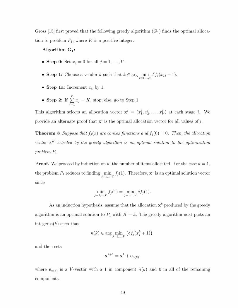
Gross [15] first proved that the following greedy algorithm (G1) finds the optimal alloca-

tion to problem P1, where K is a positive integer.

Algorithm G1:

• Step 0: Set xj = 0 for all j = 1, . . . , V .

• Step 1: Choose a vendor k such that k ∈ arg minj=1,...,V

δfj(x1j + 1).

• Step 1a: Increment xk by 1.

• Step 2: IfV∑

j=1

xj = K, stop; else, go to Step 1.

This algorithm selects an allocation vector xi = (xi1, x

i2, . . . , x

iV ) at each stage i. We

provide an alternate proof that xi is the optimal allocation vector for all values of i.

Theorem 8 Suppose that fj(x) are convex functions and fj(0) = 0. Then, the allocation

vector xK selected by the greedy algorithm is an optimal solution to the optimization

problem P1.

Proof. We proceed by induction on k, the number of items allocated. For the case k = 1,

the problem P1 reduces to finding minj=1,...,V

fj(1). Therefore, x1 is an optimal solution vector

since

minj=1,...,V

fj(1) = minj=1,...,V

δfj(1).

As an induction hypothesis, assume that the allocation xk produced by the greedy

algorithm is an optimal solution to P1 with K = k. The greedy algorithm next picks an

integer n(k) such that

n(k) ∈ arg minj=1,...,V

(

δfj(xkj + 1)

)

,

and then sets

xk+1 = xk + en(k),

where en(k) is a V -vector with a 1 in component n(k) and 0 in all of the remaining

components.

49

Let Sn = {(un1 , u

n2 , . . . , u

nV ) :

∑

uni = n} be the set of all possible allocation vectors

of n items. Consider an allocation vector uk+1 ∈ Sk+1. We claim that

V∑

j=1

fj(uk+1j ) ≥

V∑

j=1

fj(xk+1j ).

By the induction hypothesis,

δfn(k)(xk+1n(k)) ↑ in k (in the weak sense). (4.4)

Consider 1 ≤ x ≤ xk+1j for a specific vendor j. There exists an m ≤ k such that the

allocation vector xm produced by the greedy algorithm has n(m) = j, i.e.,

xm+1j = x and xm

j = x− 1.

Therefore, we have

δfj(x) = δfj(xm+1j ) = δfn(m)(x

m+1n(m)) ≤ δfn(k)(x

k+1n(k)), 1 ≤ x ≤ xk+1

j . (4.5)

The inequality above follows from 4.4. Also note that the convexity of fj gives

δfj(x) ≥ δfj(xk+1j + 1) ≥ δfn(k)(x

k+1n(k)), x > xk+1

j . (4.6)

Let A = {j : uk+1j > xk+1

j } and B = {j : uk+1j < xk+1

j }. We have:

V∑

j=1

[

fj(uk+1j ) − fj(x

k+1j )

]

=∑

j∈A

[

fj(uk+1j ) − fj(x

k+1j )

]

+∑

j∈B

[

fj(uk+1j ) − fj(x

k+1j )

]

=∑

j∈A

uk+1

j∑

x=xk+1

j+1

δfj(x) −∑

j∈B

xk+1

j∑

x=uk+1

j+1

δfj(x)

50

≥∑

j∈A

uk+1

j∑

x=xk+1

j +1

δfn(k)(xk+1n(k)) −

∑

j∈B

xk+1

j∑

x=uk+1

j +1

δfn(k)(xk+1n(k))

= δfn(k)(xk+1n(k))

∑

j∈A

uk+1

j∑

x=xk+1

j+1

1 −∑

j∈B

xk+1

j∑

x=uk+1

j+1

1

= 0.

The inequality in the fourth line comes from 4.5 and 4.6. The last equality is true because

V∑

j=1

uk+1j =

V∑

j=1

xk+1j = k + 1.

This completes the proof.

Ibaraki and Katoh [16] provide many algorithms to produce the optimal solution;

some of them run in polynomial time. The complexity of the greedy algorithm is O(V +

K logV ), since the minimization step takes O(logV ) time. It is fairly efficient; we ran

the algorithm for K = 10000 and V = 5, it took about 3 seconds on a standard machine

to run to optimality.

If the functions fj(x) are all concave, the optimum occurs at an extreme point.

The optimal solution can be found by picking the vendor j where fj(K) is minimum,

and allocating all items to vendor j. Opp, et al. [28] also discusses the case where the

functions fj(x) are mixed convex and concave; we omit that discussion in this dissertation

for the sake of brevity.

To solve the optimization problem Pm for m priority classes, we reformulate the

problem as a convex minimum cost network flow problem. In the next section, we provide

some background information on minimum cost network flow problems.

51

4.5 Minimum Cost Network Flow Problems

We first provide the background on minimum cost network flow problems with linear

costs and discuss the convex cost problem in Section 4.5.1. Let G = (N,A) be a directed

network with a cost cij and capacity uij on each arc (i, j) ∈ A. We associate each node

with a number b(i). If b(i) > 0, then b(i) indicates the supply at node i, while if b(i) < 0,

then −b(i) indicates the demand at node i. A value of b(i) = 0 implies that node i

is purely a transshipment node. We assume that∑

i

b(i) = 0, i.e. there is just enough

supply to satisfy the demand exactly. The flow from node i to node j along arc (i, j) is

denoted by xij. The objective is to find the flow x = (xij, (i, j) ∈ A) that satisfies all of

the demand at minimum cost. The problem can be stated as a linear integer program as

follows:

Minimize∑

(i,j)∈A

cijxij

subject to:∑

j:(i,j)∈A

xij −∑

k:(k,i)∈A

xki = b(i) ∀ i ∈ N (4.7)

0 ≤ xij ≤ uij and integer, ∀ (i, j) ∈ A

For a given flow x, the residual network G(x) of a graph G plays an important

role in network algorithms. To obtain G(x), we replace each arc (i, j) ∈ A by two arcs,

(i, j) and (j, i). The forward arc (i, j) has cost cij with residual capacity rij = uij − xij

and the backward arc (j, i) has cost −cij and residual capacity rji = xij.

Ahuja, Magnanti, and Orlin [1] provide many algorithms to solve minimum cost

network flow problems. We will focus on the successive shortest path algorithm found in

Section 9.7 of that book, provided below for ready reference. The algorithm uses node

52

potentials π(i) for i ∈ N . It also uses the imbalance of a node e(i), defined by

e(i) = b(i) +∑

k:(k,i)∈A

xki −∑

j:(i,j)∈A

xij, ∀ i ∈ N.

If e(i) > 0, we call node i an excess node. Similarly, if e(i) < 0, node i is a deficit node

and if e(i) = 0, the node is balanced.

Successive Shortest Path Algorithm:

initialize x := 0, π := 0, E := {i | e(i) > 0}, D := {i | e(i) < 0};

while |E| > 0 do

• select a node k ∈ E and a node l ∈ D;

• determine the shortest path distances d(j) from node k to all other nodes in the

residual network G(x) with respect to the reduced costs cπij = cij − π(i) + π(j);

• denote the shortest path from k to l by P ;

• update π := π − d;

• augment δ = min

[

e(k),−e(l), min(i,j)∈P

{rij}

]

units of flow along the path P ;

• update x, G(x), E, D and the reduced costs;

end;

Proof of optimality of the algorithm is given on page 323 of [1]. The node poten-

tials π(i) for each node are tracked to show that the reduced cost optimality conditions

are satisfied at each step of the algorithm. Therefore, once a feasible flow is obtained,

that flow is an optimal solution. However, in the actual implementation of the algorithm,

we need not track the node potentials. We justify this as follows: during each iteration

of the algorithm, we find the shortest path from an excess node to a deficit node with

respect to the reduced costs in the residual network G(x). The reduced costs are defined

53

in terms of the node potentials by

cπij = cij − π(i) + π(j), ∀ (i, j) ∈ A. (4.8)

For given excess node k and deficit node l, the cost of a path P from k to l in the residual

network is the sum of its constituent arcs. Hence

cπ(P ) = c(P ) − π(k) + π(l), ∀ paths P.

Since the shortest path from k to l has distance minPcπ(P ), the constants π(k) and π(l)

are ignored. Therefore, we can find the shortest path from k to l in the residual network

G(x) from the original arc costs and do not need to track the node potentials π or the

reduced costs cπij. Hence, the above algorithm can be simplified to:

Successive Shortest Path Algorithm:

initialize x := 0, E := {i | e(i) > 0}, D := {i | e(i) < 0};

while |E| > 0 do

• select a node k ∈ E and a node l ∈ D;

• determine the shortest path distances d(j) from node k to all other nodes in the

residual network G(x) with respect to the costs cij;

• denote the shortest path from k to l by P ;

• augment δ = min

[

e(k),−e(l), min(i,j)∈P

{rij}

]

units of flow along the path P ;

• update x, G(x), E, and D;

end;

Let n be the number of nodes and m be the number of arcs. This algorithm

terminates in at most nU iterations, where U is the largest supply of any node. Each

iteration requires solving a shortest path problem on n nodes, m arcs. Let S(n,m,C)

54

denote the time to solve a shortest path problem, where C is the maximum arc cost.

Therefore, the complexity of the successive shortest path algorithm is O(nUS(n,m, nC)),

which is pseudopolynomial in the input size since it is polynomial in n, m, and U . (Note

that nC is used rather than C in the expression, since the costs in residual network are

bounded by nC.)

Ahuja, Magnanti, and Orlin provide the capacity scaling algorithm to solve the

minimum cost network flow problem in Section 10.2 of [1], which is polynomial in the

input size. The main idea is to push flow in sufficiently large quantities to reduce the

number of augmentations required in the successive shortest path algorithm. We find

that the successive shortest path algorithm performs quite well on our networks and use

it to solve our problems.

4.5.1 Convex Network Problems

In this section we consider the convex cost case: it costs cij(x) to send a flow of x units

along the arc (i, j). The aim is to find the flow that solves the following optimization

problem:

MinimizeV∑

j=1

cij(xij)

subject to:∑

j:(i,j)∈A

xij −∑

k:(k,i)∈A

xki = b(i) ∀ i ∈ N (4.9)

0 ≤ xij ≤ uij and integer, ∀ (i, j) ∈ A

This case can be handled similarly to the linear cost case, with a slight modifica-

tion of the network. We achieve this transformation by breaking the convex cost function

cij(x) into a piecewise linear function consisting of uij pieces, with the breakpoints oc-

curing at each integer point between 1 and uij. Replace each arc (i, j) in the network G

by uij parallel arcs. The kth arc (i, j)k has capacity 1 and cost ckij = cij(k) − cij(k − 1)

55

(k = 1, . . . , uij). Let ykij be the flow on arc (i, j)k, hence

xij =

uij∑

k=1

ykij.

Therefore, we can formulate the convex minimum cost network flow problem as the

following integer linear program:

Minimize∑

(i,j)∈A

uij∑

p=1

cpijypij

subject to:∑

j:(i,j)∈A

uij∑

p=1

ypij −

∑

k:(k,i)∈A

uki∑

p=1

ypki = b(i) ∀ i ∈ N

0 ≤ ypij ≤ 1 and integer, ∀ (i, j) ∈ A, p = 1, . . . , uij.

Since this formulation has only linear costs, we can use the successive shortest path

algorithm to solve it. In practice, we do not need to physically replace each arc by

uij parallel arcs. The convexity of the cost function implies that the arc costs ckij are

increasing in k. When a unit of flow is sent from i to j along a shortest path, the flow

will go on the arc of lowest cost. If the current amount of flow from i to j is xij, the cost

of sending one additional unit of flow from i to j is

cij(xij + 1) − cij(xij).

Therefore, we can use the successive shortest path algorithm to solve the convex cost

problem by just updating the cost on arc (i, j) at each iteration as cij(xij + 1)− cij(xij).

We point out that a similar method as the capacity scaling algorithm will solve the convex

problem in polynomial time, given in Section 14.5 of [1].

56

4.6 Network Flow Formulation

We next show that the optimization problem Pm can be reformulated as a network flow

problem. We begin with the single priority case.

4.6.1 Single Priority Class

In section 4.4, we discussed the single priority case and showed that the greedy algorithm

G1 provides an optimal solution. Here we reformulate the problem as a convex minimum

cost network flow problem. Consider the network shown in Figure 4.1 below. The source

ONMLHIJK1

��999

9999

9999

9999

9999

9999

9

ONMLHIJK2

%%KKKKKKKKKKKKKKKKK

GFED@ABCs

BB������������������������

99sssssssssssssssss//

��:::

::::

::::

::::

::::

::::

ONMLHIJK3 // GFED@ABCt

...

ONMLHIJKV

AA�����������������������

Figure 4.1: Network Model of Single Priority Problem

node s has a supply of K units and the sink node t has a demand of K units, i.e.

b(s) = K, b(t) = −K, and b(j) = 0 (j = 1, . . . , V ). Each of the arcs (s, j) (j = 1, . . . , V )

has capacity usj = K and cost csj(x) = 0 ∀x. Each arc (j, t) (j = 1, . . . , V ) has capacity

K and cost function cjt(x) = fj(xj), where xj is the flow along arc (j, t) (which equals

the flow along (s, t)) and represents the number of items assigned to server j. The integer

57

linear program developed in 4.9 reduces to:

minV∑

j=1

fj(xj)

stV∑

j=1

xj = K

0 ≤ xj ≤ K and integer, j = 1, . . . , V

Therefore, the network formulation of the problem is equivalent to the original single-

priority problem P1. We apply the successive shortest path algorithm to solve this mini-

mum cost network flow problem for this network. The algorithm significantly simplifies

since there is only 1 deficit node and 1 excess node and the shortest path step is very

easy. At each iteration there are only V paths from s to t (the residual network has no

negative cycles). The cost to send one additional unit of flow through node j when there

is already a flow of xj is δfj(xj + 1). Hence the algorithm given in section 4.5 to solve

the network problem reduces to:

Successive Shortest Path Algorithm for 1-priority:

initialize x := 0;

whileV∑

j=1

xj < K do

• compute minj=1,...,V

δfj(xj + 1)

• increment xk by 1, where k ∈ arg minj=1,...,V

δfj(xj + 1);

end

This is exactly the same as the G1 algorithm given in Section 4.4, and therefore

we have another proof of correctness of the algorithm. As stated in Section 4.4, the

complexity of this algorithm is O(V +K log V ).

58

4.6.2 Two Priority Classes

We next turn to the two priority problem. The network model for this problem is provided

in Figure 4.2 below. The source node s1 has a supply of b(s1) = K1 units, node s2 has

ONMLHIJK1

��999

9999

9999

9999

9999

9999

9

ONMLHIJKs1

99rrrrrrrrrrrrrrrrr//

%%LLLLLLLLLLLLLLLLL

��111

1111

1111

1111

1111

1111

1111

1111

11ONMLHIJK2

%%KKKKKKKKKKKKKKKKK

ONMLHIJK3 // GFED@ABCt

ONMLHIJKs2

FF

BB������������������������

88rrrrrrrrrrrrrrrrr

%%LLLLLLLLLLLLLLLL...

ONMLHIJKV

BB�����������������������

Figure 4.2: Network Model of Two-priority Problem

a supply of b(s2) = K2 units, and the sink node t has a demand of K1 + K2 units (i.e.

b(t) = −(K1 + K2)). All other nodes j are transshipment nodes and have b(j) = 0

(j = 1, . . . , V ). Let xij be the flow from node si to node j (i = 1, 2), which represents the

number of type i customers assigned to server j. The arcs have the following capacities,

flows, and costs (j = 1, . . . , V ):

Arc Capacity Flow Cost(s1, j) K1 x1j f1j(x1j)(s2, j) K2 x2j 0(j, t) K1 +K2 x1j + x2j f2j(x1j + x2j)

Table 4.1: Arc Properties for Two-priority Network

59

The minimum cost network flow problem defined in 4.9 reduces to:

MinimizeV∑

j=1

[f1j(x1j) + f2j(x1j + x2j)]

subject to:V∑

j=1

x1j = K1,V∑

j=1

x2j = K2,

0 ≤ xij ≤ Ki and integer, i = 1, 2, j = 1, . . . , V.

This is equivalent to the optimization problem P2; hence we can apply the successive

shortest path algorithm to this network shown in Figure 4.2 to solve the two-priority

problem. Like the single-priority case, the network structure for the two-priority problem

simplifies the successive shortest path algorithm significantly. Now there are two excess

nodes; without loss of generality we start with node s2, pushing K2 units of flow to the

sink t. Since node s1 is not accessible from node s2, we can omit s1 and all of the arcs

incident with it from the network. Thus we determine x2j (j = 1, . . . , V ) by the G1

algorithm on this reduced network. Next we return to the original network and push

the K1 units of flow from the source s1 to the sink t. Here there are V + 1 paths in

the residual network G(x) to consider. There are V direct paths to t through node j

(j = 1, . . . , V ). The cost of these paths are δf1j(x1j + 1) + δf2j(x1j + x2j + 1). Another

possible shortest path to t goes through s2. The shortest path from s1 to s2 is through

a node k such that

k ∈ arg minx2j>0

δf1j(x1j + 1)

Note that the cost of pushing flow from j to s2 is 0 if x2j > 0. From s2 to the sink t, the

shortest path is determined by choosing a vendor m such that

m ∈ arg minjδf2j(x1j + x2j + 1).

60

Augmenting a unit of flow along this path requires that we increase x1k and x2m by 1

unit and decrease x2k by 1 unit. Therefore, we have the following algorithm to solve the

two-priority problem:

Successive Shortest Path Algorithm for 2-priority (Algorithm G2):

initialize x := 0;

whileV∑

j=1

x2j < K2 do

• compute minj=1,...,V

δf2j(x2j + 1)

• increment x2k by 1, where k ∈ arg minj=1,...,V

δfj(x2j + 1);

end

whileV∑

j=1

x1j < K1 do

• compute dj = δf1j(xj + 1) + δf2j(x1j + x2j + 1), j = 1, . . . , V and

dV +1 = minx2j>0

δf1j(x1j + 1) + minkδf2k(x1k + x2k + 1).

• let q ∈ arg minj=1,...,V +1

dj.

If q ∈ {1, . . . , V }, increment x1q by 1.

If q = V + 1, let k ∈ arg minx2j>0

δf1j(x1j + 1) and p ∈ arg minjδf2j(x1j + x2j + 1).

Increment x1k and x2p by 1 and decrement x2k by 1 unit.

end

This algorithm has the advantage of being very easy to code. It is very similar to the

greedy algorithm G1 since it adds one item at a time, with the possibility of rearranging

the lower priority items previously assigned. The complexity of the algorithm is O(V +

K logV ).

4.6.3 Multiple Priority Classes

We now address the m priority problem. The network model for this problem is provided

in Figure 4.3. This network has m source nodes, labeled s1, s2, . . ., sm, with node si

61

WVUTPQRS11 // · · · // _^]\XYZ[1m−1

��:::

::::

::::

::::

::::

::

ONMLHIJKs1

99rrrrrrrrrrrrrr//

%%LLLLLLLLLLLLLL

��111

1111

1111

1111

1111

1111

1111

1WVUTPQRS21 // · · · // _^]\XYZ[2m−1

&&LLLLLLLLLLLLLL

ONMLHIJKs2

BB���������������������

99rrrrrrrrrrrrrr//

��;;;

;;;;

;;;;

;;;;

;;;;

WVUTPQRS31 // · · · // _^]\XYZ[3m−1 // GFED@ABCt

......

......

WVUTPQRSsm

<<xxxxxxxxxxxxxxxxxxxxxxxxxxxxxxxxxxxxxxxxxxxxxxxxxxxxxxx

88rrrrrrrrrrrrrrrrrrrrrrrrrrrrrrrrrrrrrrrrrrrrrrrrrr

55kkkkkkkkkkkkkkkkkkkkkkkkkkkkkkkkkkkkkkkkkkkkk

44WVUTPQRSV 1 // · · · // _^]\XYZ[V m−1

@@��������������������

Figure 4.3: Network Model of m Priority Problem

having supply Ki (i.e. b(si) = Ki for i = 1, . . . , m). There is a single sink node t that

has demandm∑

i=1

Ki, i.e. b(t) = −m∑

i=1

Ki. There are m− 1 nodes for each vendor j (labeled

j1, . . . , jm−1) such that b(ji) = 0. The node s1 is connected with nodes j1 (j = 1, . . . , V ).

Similarly, si is connected with nodes ji−1 (i = 2, . . . , m, j = 1, . . . , V ). The node ji is

connected with node ji+1 (i = 1, . . . , m − 2, j = 1, . . . , V ). Let x1j be the flow from

node s1 to node j1 and xij be the flow from node si to node ji−1 (i = 2, . . . , m). The

flow xij gives the number of type i items assigned to server j. We continue using the

notation thatp∑

i=1

xij = Xpj. Due to the flow balance constraints, the flow on arc (j i, ji+1)

is Xi+1,j and the flow on arc (jm−1, t) is Xmj. The arcs capacities, flows, and costs are

summarized in Table 4.2 (j = 1, . . . , V in each row):

62

Arc Capacity Flow Cost(s1, j

1) K1 x1j f1j(x1j)(si, j

i−1) Ki xij 0 (i = 2, . . . , m)

(ji, ji+1)i+1∑

p=1

Kp Xi+1,j fi+1,j(Xi+1,j) (i = 1, . . . , m− 1)

(jm−1, t)m∑

p=1

Kp Xmj fmj(Xmj)

Table 4.2: Arc Properties for m-priority Network

We now give the minimum cost network flow formulation defined in 4.9 for this

network:

min

V∑

j=1

fj(x1j , x2j , . . . , xmj)

s.t.V∑

j=1

xij = Ki, i = 1, . . . , m

0 ≤ xij ≤ Ki, and integer; i = 1, . . . , m, j = 1, . . . , V

where fj(x1j , x2j , . . . , xmj) =∑m

p=1 fpj(Xpj). Note that this is the same formulation that

we developed in Section 4.3. Hence, we can apply the successive shortest path algorithm

to this network to solve the m-priority problem. The network G has m + 1 + (m− 1)V

nodes and (2m−1)V arcs. We turn to one of the well-established shortest path algorithms

to find the shortest path at each iteration of the algorithm. We start pushing flow from

sm to t in the reduced network Gm, ignoring the other source nodes and the arcs incident

with it. In general, we refer to the reduced network that omits the source nodes s1

through si−1 and their incident arcs by Gi. Next, we push flow from sm−1 to t in the

reduced network Gm−1. This procedure continues until we push the flow from s1 to t over

the full network in Figure 4.3. We outline the algorithm to solve the m-priority problem

below:

63

Successive Shortest Path Algorithm for m-priority (Algorithm Gm):

initialize x := 0;

for i = m to 1 whileV∑

j=1

xij < Ki do

• determine the shortest path P from node si to node t in the residual network Gi(x)

constructed from the reduced network Gi;

• augment 1 unit of flow along the path P ;

• update x and Gi(x);

end while loop;

end for loop;

The residual graph Gi(x) has at most N = m+ 1 + (m− 1)V nodes and at most

A = 2(2m− 1)V edges. We use the label correcting algorithm to solve the shortest path

problem at each iteration; it has complextiy O(NA), where N is the number of nodes

and A is the number of arcs. Therefore, this algorithm has complextiy O(m2KV 2) (since

from NA ≈ 4m2V 2). Typical parameters values are m ∈ {1, . . . , 4} and V ∈ {1, . . . , 10}.

With these parameters, the algorithm is quite efficient. For an example with m = 4,

V = 6, and K = 10000, the algorithm took about 15 seconds on a standard machine.

4.7 Computational Issues

In this section, we discuss some of the computational issues related to the outsourcing

problem. First, we compute the expected queue length in a M/M/sj/ · /N finite popula-

tion queue. The easiest case is when sj = 1 ∀j. We derive the steady-state probabilities

for exponential lifetimes and use the result of Bunday and Scranton [8] that these are

the same steady state probabilities when item lifetimes are not exponentially distributed.

64

The state space is {0, 1, . . . , N} with transition rates

λi = (N − i)λ, 0 ≤ i ≤ N

µi = µ, 1 ≤ i ≤ N.

Let pi be the long-run probability that the queue has i items, including the item in

service. Solving the balance equations for pi, we get the recurrence relation

pi+1 =N − i

ρpi 0 ≤ i ≤ N − 1, (4.10)

where ρ = µ/λ. The expected queue length L(N) can be computed by

N − L(N) =N∑

i=0

(N − i)pi.

We use Equation 4.10 to compute L(N). We have

N − L(N) =

N∑

i=0

N − i

ρi(N − i)!

/

N∑

j=0

1

ρj(N − j)!

= ρ

(

N∑

i=0

1

ρi(N − i)!−

1

N !

)/

N∑

j=0

1

ρj(N − j)!

= ρ−ρ/N !

N∑

j=0

1/ (ρj(N − j)!)

= ρ− ρρN/N !N∑

j=0

ρj/j!

= ρ− ρB(ρ,N),

where

B(ρ,N) =ρN/N !N∑

j=0

ρj/j!

65

is the Erlang Loss function (see [19]). Therefore, we use

L(N) = N − ρ+ ρB(ρ,N) (4.11)

to compute the expected queue length. When N is large, directly calculating B(ρ,N) is

difficult. Therefore, we use the following recursion to compute B(ρ,N):

B(ρ,N) =ρB(ρ,N − 1)/N

1 + ρB(ρ,N − 1)/N, N ≥ 1, (4.12)

where B(ρ, 0) = 1.

Opp, et al. [28] dedicates a section to discussing calculation issues when there

are multiple servers at each vendor; we omit it for the sake of brevity. They show that

a queue with sj servers working at rate µj can be well approximated by a single server

queue working at rate sjµj. This approximation works best when the servers are rarely

idle, which is common in practice. If the exact expected queue length is needed when

sj > 1 for some j, we can use an analysis of a two station closed queueing network, given

in Section 2.7 of Gross and Harris [14]. Opp [27] gives a recursive method of computing

the expected queue length in this case. We provide those results here for ready reference.

Consider a two-station closed queueing network, station 1 an infinite server station

with service rate λ and station 2 is a s server station with service rate µ per server. There

are N items circulating continuously in the network between stations 1 and 2 (assume

that N ≥ s). We calculate the expected number of customers at station 2. Let ρ = sµ/λ.

Then, the probability that all s servers at station 2 are busy, and hence the probability

that an incoming item is blocked, is given by

PB(N) =

∑N−s

i=0 ρi/i!∑N−s

i=0 ρi/i! + A(N)ρN−s/(N − s)!, (4.13)

66

where

A(N) =

s∑

i=1

ρis!/(s− i)!

si(N − s+ i)!/(N − s)!.

Note that A(N) has only s terms, so we need not compute it recursively. Clearly PB(N) =

0 for N < s. From Equation 4.13, we get the following expression for PB(N) in terms of

A(N) and B(ρ,N):

PB(N) =1

1 + A(N)B(ρ,N − s).

Recall that B(ρ,N − s) can be computed recursively from Equation 4.12.

Let Wq(N) by the mean waiting time in the queue at station 2 with N customers

circulating in the network. Similarly, define Lq(N) as the expected number of customers

waiting in the queue at station 2 and L(N) as the expected number of customers in the

queue at station 2. The following recursion holds (initialize Lq(0) = 0):

Wq(N) =PB(N − 1) + Lq(N − 1)

sµ,

Λ(N) =N

1/λ+ 1/µ+Wq(N),

Lq(N) = Λ(N)Wq(N), and

L(N) = Lq(N) + Λ(N)/µ.

4.8 An Example

We provide an example to illustrate the Gm algorithm. Consider a manufacturer that

has warrantied items of m = 4 different priority types. The number of items of each

priority type is K1 = 150, K2 = 250, K3 = 200, and K4 = 400 (for a total of 1000 items).

Each item has a common failure rate of λ = 1.5 failures per year. There are V = 6

vendors at his disposal. Typically, each repairperson at a vendor is busy with repairs

during the majority of the time. Hence, we use the result stated in the previous section

that s repairpeople working at rate µ is very similar to a single repairperson working at

67

rate sµ. For this reason, we assume that there is a single repairperson working at rate

sjµj at each vendor j. The vendors’ properties are summarized in Table 4.3.

Vendor j sjµj cj (h1j , h2j, h3j , h4j)1 80 15 (500, 350, 300, 175)2 62 19 (500, 400, 250, 175)3 70 18 (500, 350, 300, 160)4 50 15 (500, 400, 250, 160)5 45 14 (500, 400, 300, 175)6 25 9 (500, 350, 300, 175)

Table 4.3: Costs and Service Rates for Each Vendor

Note that for every vendor j, hij > hi+1,j (i = 1, . . . , 3) and h4j > λcj, so the

convexity properties for the fij functions are satisfied. We apply the Gm algorithm on

these parameters. The allocation matrix below is the solution, where the row indicates

the priority type and the column indicates the vendor. For example, the number of type

3 items assigned to server 4 is 80.

X =

39 34 31 24 21 1

62 33 56 30 33 36

0 120 0 80 0 0

0 0 300 95 5 0

The expected yearly cost of this allocation is $146, 012.42.

4.9 Cost Benefits of the Multi-Priority Approach

In this section, we discuss the benefits of giving priority in service to items that have

higher holding costs. We first illustrate the benefits on the example in the previous

section. Suppose there was no priority structure in place, but the holding costs are still

given as in Section 4.8. Consider a specific vendor j. If N items are randomly assigned to

68

vendor j ignoring priority levels, the expected number of type i items assigned to server

j is:

Ki

m∑

i=1

Ki

N.

If there is no priority structure, the expected waiting time will be independent of the

priority type. Therefore, the expected holding cost per item hj assigned to server j is

hj =

K1Nm∑

i=1

Ki

h1j + . . .+KVNm∑

i=1

Ki

hV j

/

N =

m∑

i=1

Kihij

m∑

i=1

Ki

. (4.14)

We apply the formula in 4.14 to get the following average holding costs for the vendors

in the Example in Section 4.8:

Vendor j 1 2 3 4 5 6

hj 292.5 295 286.5 289 305 292.5

Table 4.4: Average Holding Costs for Vendors

Now we solve the single priority problem with the holding costs from Table 4.4, and

repair costs and service rates from Table 4.3 on K = 1000 items. The optimal allocation

vector is (106, 83, 637, 73, 61, 40) and the long-run average yearly cost is $197, 520.56.

This represents a 35.3% increase over the cost with the priority structure in place. The

reason for the increase is that the higher priority items are in service for a longer portion

of time and hence create a higher overall holding cost.

We next turn to an example where there are only two priority classes and their

holding costs differ by only 10%. We consider 5 vendors and 10, 000 total items, with

K1 = 2500 and K2 = 7500, so the majority of the items are low priority items. The items

fail at rate 2 per year. The 5 vendors have the following properties:

69

Vendor j 1 2 3 4 5cj 20 18 23 16 25sjµj 1000 200 400 600 700h1j 220 203.5 198 231 209h2j 200 185 180 210 190

hj 205 189.62 184.5 215.25 194.75

Table 4.5: Vendor Properties for Similar Cost Example

When the type 1 items are not given priority in service, the allocation vector is

(1063, 238, 7293, 644, 762) and the total long-run average cost is $1, 374, 210 per year. On

the other hand, when the type 1 items are given priority in service we apply the Gm

algorithm, which produces the following allocation matrix:

X =

890 152 335 512 611

173 86 6958 132 151

.

In this case, the long-run average cost is $1, 342, 645 per year. The cost savings using

the priority structure is 2.35%. Note that in this example the total number of items

allocated to each vendor is the same regardless of the priority structure used. There are

other examples where the total allocation does depend on the priority structure (e.g. the

previous example). Clearly the priority structure is more beneficial when high priority

items dramatically affect the holding cost. However, even in the case of similar holding

costs among the different priority types, the priority structure can reduce cost by a small

amount with relatively little effort.

4.10 Selecting the Values of Ki

Suppose that the manufacturer has K items to sell. The manufacturer has the option of

offering up to m different warranty contracts. The contracts dictate the priority level,

i.e. the most expensive contract will guarantee first priority in service, the second most

70

expensive contract guarantees second priority in service, etc. The manufacturer charges

the customer ri dollars for each item to have a type i priority in service (i = 1, . . . , m).

We assume that rm = 0 for the standard lowest priority warranty, and ri > ri+1 for

i = 1, . . . , m − 1. The values of ri are fixed and are determined by the competition

and the manufacturer cannot control these. We assume that the manufacturer can sell

any number of items under any warranty contract. That is, he will sell all of the items

regardless of the warranty contract(s) he offers. Typically, these assumptions are satisfied

if the manufacturer is a small player in a large market.

Now, the manufacturer must decide on the values of Ki (i = 1, . . . , m) in addition

to the optimal allocation matrix. The optimization problem is:

minV∑

j=1

fj(x1j , x2j , . . . , xmj)

s.t.

m∑

i=1

Ki = K,

V∑

j=1

xij = Ki, i = 1, . . . , m

xij, Ki ≥ 0, and integer; i = 1, . . . , m, j = 1, . . . , V

where fj(x1j , x2j , . . . , xmj) =∑m

p=1 (fpj(Xpj) − rpKp). We can model the problem as a

minimum cost network flow problem, similar to the problem discussed in Section 4.6.3

with the addition of a single node S that is connected to each of the nodes si, i = 1, . . . , m.

The node S is the single source node with b(S) = K. The nodes si (i = 1, . . . , m) are

now transshipment nodes, i.e. b(si) = 0. The arcs (S, si) have capacity K and cost −ri.

The rest of the network is the same as described in Section 4.6.3. We provide the network

diagram in Figure 4.4.

71

WVUTPQRS11 // · · · // _^]\XYZ[1m−1

��:::

::::

::::

::::

::::

::

ONMLHIJKs1

99rrrrrrrrrrrrrr//

%%LLLLLLLLLLLLLL

��111

1111

1111

1111

1111

1111

1111

1WVUTPQRS21 // · · · // _^]\XYZ[2m−1

&&LLLLLLLLLLLLLL

ONMLHIJKS

99ssssssssssssss//

��:::

::::

::::

::::

::::

ONMLHIJKs2

BB���������������������

99rrrrrrrrrrrrrr//

��;;;

;;;;

;;;;

;;;;

;;;;

WVUTPQRS31 // · · · // _^]\XYZ[3m−1 // GFED@ABCt

......

......

WVUTPQRSsm

<<xxxxxxxxxxxxxxxxxxxxxxxxxxxxxxxxxxxxxxxxxxxxxxxxxxxxxxx

88rrrrrrrrrrrrrrrrrrrrrrrrrrrrrrrrrrrrrrrrrrrrrrrrrr

55kkkkkkkkkkkkkkkkkkkkkkkkkkkkkkkkkkkkkkkkkkkkk

44WVUTPQRSV 1 // · · · // _^]\XYZ[V m−1

@@��������������������

Figure 4.4: Network Model of Reward Problem

For ready reference, we provide the entire set of arc properties in Table 4.6:

Arc Capacity Flow Cost(S, si) K Ki −ri (i = 1, . . . , m)(s1, j

1) K x1j f1j(x1j)(si, j

i−1) Ki xij 0 (i = 2, . . . , m)

(ji, ji+1)i+1∑

p=1

Kp Xi+1,j fi+1,j(Xi+1,j) (i = 1, . . . , m− 1)

(jm−1, t)m∑

p=1

Kp Xmj fmj(Xmj)

Table 4.6: Arc Properties for the Reward Network

We apply the successive shortest path algorithm to solve this problem by contin-

ually augmenting one unit of flow along the shortest path from S to t. Note that there

are still no negative cycles in the graph. We illustrate the problem with an example.

Example 4.1 Consider the example of Section 4.8, with ri = (15, 10, 5, 0). Here are

the parameters of the problem:

72

Vendor j sjµj cj (h1j , h2j, h3j , h4j)1 80 15 (500, 350, 300, 175)2 62 19 (500, 400, 250, 175)3 70 18 (500, 350, 300, 160)4 50 15 (500, 400, 250, 160)5 45 14 (500, 400, 300, 175)6 25 9 (500, 350, 300, 175)

Table 4.7: Costs and Service Rates for Each Vendor

Recall that the original values of Ki were (150, 250, 200, 400) and the expected

yearly cost was $146, 012.42. If we use these values of Ki with the above values of ri, the

expected yearly cost is now $140, 262.40 after deducting the additional policy costs that

the manufacturer charges. However, using the successive shortest path algorithm gives

us an optimal allocation of

X =

34 25 27 17 16 0

13 0 10 0 0 6

0 11 0 6 0 0

52 42 573 95 43 30

,

with K = (119, 29, 17, 835). The cost of allocation is $112, 326.61, a 20% reduction in

cost over the previous solution. In this example, it is optimal for the manufacturer to

offer all four warranty types. However, this may not occur in every example.

73

Chapter 5

Conclusions and Future Work

In this dissertation, we investigated two problems in warranty cost analysis. First, we

addressed the problem of modeling a warranty reserve where contributions are made after

each sale (where the sales process is a nonhomogeneous Poisson process). We derived

the mean and variance of the reserve for all time points t and offered a heuristic for

determining good values of c, the contribution amount after each sale, and R0, the initial

reserve level. We also provided extensions of the model by allowing a random contribution

amount and multiple products from the same manufacturer. Next, we addressed the

problem of outsourcing warranty repairs when items have priority in service. We provided

the known result for the single priority case and used a network flow model to solve the

multi-priority problem. We also provided a numerical comparison of the single-priority

problem versus the multi-priority problem.

There are many extensions of our basic warranty reserve model for future research.

One simple extension is to allow a fluctuating interest rate. We mention several other

extensions below:

74

• Bulk arrivals: The sales occur in batches with a common probability distribu-

tion. The successive batch arrivals are independent of each other, but the warranty

periods within each batch may be dependent.

• Ruin Probability: A common problem in risk theory is to compute the probability

of ruin prior to time t. That is, we want to analytically compute the probability,

in terms of the problem parameters, that the reserve account drops below a given

amount B > 0 prior to time t. Asmussen [3] provides an extensive reference on ruin

probabilities. However, the specific case of premiums depending on the number of

items or policies is not addressed.

• Reserve-dependent Contributions: We allow the reserve contribution to de-

pend on the reserve level and the number of items under warranty. There are two

possible approaches: to determine a contribution function c(R(t), X(t)) prior to

time 0 that can be applied for the entire fiscal period, or to dynamically determine

the contribution amount at time t.

• Criteria for Selecting c and R0: In this dissertation, we selected c and R0 so the

reserve level remains above a target B with approximate 100(1 − β)% probability.

We can consider other objectives for the manufacturer, such as minimizing a penalty

function. That is, if the reserve falls below the target B, the manufacturer incurs

sanctions as a function of the time below the target and the amount below the

target.

• Other Applications: We believe adaptations of our reserve management model

can be applied to pension funds and insurance accounts. Currently, the literature

on these subjects considers a constant premium input and a static number of cus-

tomers. For pension funds, we would track the workers currently eligible for pension

and the workers eligible for pension in the future. The contribution amount can

be a function of both of these, while the subtraction amount will depend on the

75

former. The insurance model would consider many classes of customers (as our

model allows), but may have different failure distributions.

The second problem we addressed in this dissertation is the static allocation of

prioritized warranty repairs. Some extensions of the static allocation model include:

• Different Priority Structures: We can consider other priority structures, such

as non-preemptive priority. In this case, the computation of the expected queue

lengths is more complicated and we lose the special structure of the objective.

• Enforce Maximum Waiting Times: If the contracts specify a maximum repair

turnaround time for the different priority types, we should incorporate this into the

model.

• Simulation: We can use simulation to determine if our allocation strategy per-

forms well under different failure and service distributions.

• Game Theoretic Problems: In our research, we assumed that the manufacturer

pays a fixed fee per repair to each vendor. Often these contracts are negotiated

between the manufacturer and the vendor and may depend on the number of items

allocated to that vendor.

• Dynamic Allocation: Another possible allocation strategy is dynamic allocation,

i.e. the items are allocated only after a claim is made. Opp [27] uses index policies

to address the single priority case. We are interested in how index policies can be

used to estimate the optimal solution in the multi-priority case.

76

Bibliography

[1] R. K. Ahuja, T. L. Magnanti, and J. B. Orlin. Network Flows: Theory, Algorithms,and Applications. Prentice Hall, New Jersey, 1993.

[2] H. N. Amato and E. E. Anderson. Determination of warranty reserves: an extension.Management Science, 22(12):1391–1394, 1976.

[3] S. Asmussen. Ruin Probabilities. World Scientific, Singapore, 2000.

[4] Y. Balcer and I. Sahin. Replacement costs under warranty: Cost moments and timevariability. Operations Research, 34(4):554–559, 1986.

[5] W. R. Blischke and D. N. P. Murthy. Warranty Cost Analysis. Marcel Dekker, NewYork, 1994.

[6] K. M. Bretthauer and B. Shetty. The nonlinear resource allocation problem. Oper-ations Research, 43(4):670–683, 1995.

[7] K. M. Bretthauer and B. Shetty. The nonlinear knapsack problem - algorithms andapproaches. European Journal of Operations Research, 138(3):459–472, 2002.

[8] B. D. Bunday and R. E. Scranton. The G/M/r machine interference model. Euro-pean Journal of Operations Research, 4:399–402, 1980.

[9] H. Cramer. Collective Risk Theory. Esselte Reklam, Stockholm, 1955.

[10] L. W. Dowdy, D. L. Eager, K. D. Gordon, and L. V. Saxton. Throughput concavityand response time convexity. Information Processing Letters, 19:209–212, 1984.

[11] S. G. Eick, W. A. Massey, and W. Whitt. The physics of the Mt/G/∞ queue.Operations Research, 41(4):731–742, 1993.

[12] J. Eliashberg, N. D. Singpurwalla, and S. P. Wilson. Calculating the warranty reservefor a time and usage indexed warranty. Management Science, 43(7):966–975, 1997.

[13] T. S. Glickman and P. D. Berger. Optimal price and protection period decisions fora product under warranty. Management Science, 22:1381–1390, 1976.

[14] D. Gross and C. M. Harris. Fundamentals of Queueing Theory. Wiley, secondedition, 1985.

[15] O. Gross. A class of discrete type minimization problems. Technical Report RM-1644, RAND Corporation, 1956.

[16] T. Ibaraki and N. Katoh. Resource Allocation Problems: Algorithmic Approaches.MIT Press, Cambridge, MA, 1988.

77

[17] S. S. Ja. Computation of warranty reserves for non-stationary sales processes. PhDthesis, University of North Carolina at Chapel Hill, 1998.

[18] S. S. Ja, V. G. Kulkarni, A. Mitra, and J. F. Patankar. Warranty reserves fornon-stationary sales processes. Naval Research Logistics, 49(5):499–513, 2002.

[19] D. L. Jagerman. Some properties of the erlang loss function. The Bell SystemTechnical Journal, 53(5):525–551, 1974.

[20] A. A. Jagers and E. A. V. Doorn. On the continued Erlang loss function. OperationsResearch Letters, 5:43–46, 1986.

[21] A. Y. Khintchine. Mathematical Models in the Theory of Queueing (in Russian).Trudy Mat Inst. Steklov 49, 1955. English translation by Charles Griffin and Co.,London, 1960.

[22] S. A. Klugman, H. H. Panjer, and G. E. Willmot. Loss Models: From Data toDecisions. Wiley, 1998.

[23] J. W. Mamer. Cost analysis of pro rate and free-replacement warranties. NavalResearch Logistics Quarterly, 29:345–356, 1982.

[24] J. W. Mamer. Discounted and per unit costs of product warranty. ManagementScience, 33(7):916–930, 1987.

[25] W. W. Menke. Determination of warranty reserves. Management Science,15(10):542–549, 1969.

[26] E. J. Messerli. Proof of a convexity property of the Erlang B formula. Bell SystemTechnical Journal, 51:951–953, 1972.

[27] M. Opp. Outsourcing Warranty Repair Services. PhD thesis, University of NorthCarolina at Chapel Hill, 2003.

[28] M. Opp, I. Adan, V. G. Kulkarni, and J. M. Swaminathan. Outsourcing warrantyrepairs: Static alloation. Technical Report 03-01, University of North Carolina atChapel Hill, 2003. Submitted to Management Science.

[29] C. Palm. Intensity variations in telephone traffic (in german). Ericcson Technics,44:1–189, 1943. English translation by North-Holland, Amsterdam, 1988.

[30] T. Rolski, H. Schmidli, V. Schmidt, and J. Teugels. Stochastic Processes for Insur-ance and Finance. Wiley, Chichester, England, 1999.

[31] L. Takacs. Introduction to the Theory of Queues. Oxford University Press, NewYork, 1962.

[32] C. S. Tapiero and M. J. Posner. Warranty reserving. Naval Research Logistics,35:473–479, 1988.

78

[33] U.S. Federal Trade Commission Improvement Act (1975). 88 Stat 2183, Washington,DC, 101–112.

[34] A. Zaporozhets. A short proof of optimality of the bottom up algorithm for discreteresource allocation problems. Operations Research Letters, 21(2):81–85, 1997.

79