manual on tax analysis and revenue forecasting:...
TRANSCRIPT

Manual on Tax Analysis and Revenue Forecasting – Draft, August 2008 Page 1 of 34
Manual on Tax Analysis and Revenue Forecasting: Outline
Jonathan Haughton1
Suffolk University, Boston
August 2008
Introduction
Tax analysis addresses the question of what effects changes in tax policy – especially tax rates and bases
– will have on government revenue, and on the distribution of income (“incidence”). Revenue forecasting
is concerned with estimating government revenue in the future, given current tax law.
When discussing whether taxes should be changed or reformed, good revenue forecasts and clear tax
analyses are essential. In the United States, information on potential tax changes is often produced
quickly in the form of two-page “revenue notes”, which then circulate to lawmakers as they consider
revisions to the law.
The purpose of this manual is to set out the most important methods that are typically used for tax
analysis and revenue forecasting, along with worked examples and practice exercises. Anyone who
works though this manual should be able to begin to make sensible revenue forecasts, and begin to
undertake sound tax analysis.
This is a preliminary version of the Manual, and comments are most welcome. Please send them to
Jonathan Haughton at [email protected] .
Types of Revenue Estimation and Forecasting
It is helpful to separate the analysis into three parts, which we treat in turn in the sections that follow.
a. Short-Term Cash Receipts Forecasting Models
The purpose here is to forecast cash receipts from taxes over the months ahead, but not more than two
years into the future. This is useful for the purposes of cash management – so that the treasury can
determine how much to borrow in the short run, or how much revenue will be available to fund
expenditure initiatives.
For example, every December, the Ways and Means Committee of the Commonwealth of Massachusetts
(USA), which oversees revenue and spending, convenes a meeting at which a few experts are invited to
make projections of revenue for the rest of the fiscal year (which ends on June 30) and the following
fiscal year. After deriving a “consensus” forecast based on these projections, the committee is then able
to tailor its spending projects for the subsequent year or two. Appendix xxx reproduces the submission to
the committee that was made by the Beacon Hill Institute in December 2007; it also includes a useful
summary of the methodology used.
In practice, such short-term forecasts are typically based on monthly data for the previous several years,
augmented with some information about recent changes in the tax code. The forecasts themselves are
1 Thanks are due to Ngo Viet Phuong who helped develop some of the material and exercises related to the section
on short-term forecasting.

Manual on Tax Analysis and Revenue Forecasting – Draft, August 2008 Page 2 of 34
then made using simple forecasting methods, or more elaborate techniques such as Autoregressive
Integrated Moving Averages (ARIMA), which are explained more fully below.
b. Medium-term forecasting models
The purpose here is to forecast revenue, annually, for a period of anything from about one to ten years.
This is needed for medium- and long-term budgeting, and is one of the staple activities of budget
departments.
The commonest approach is forecast revenue separately for each major tax. In each case one identifies a
base (such as GDP or consumption) for which forecasts are available, constructs a “clean” series of tax
payments that correct for changes in tax rules over time, links tax revenue from this clean series to the
base, and then extrapolates the growth of the base, and hence revenue, into the future.
c. Tax policy analysis models
In considering changes to the tax code, it is important to know what the effects will be on (i) government
revenue, and (ii) the true incidence of the tax. The incidence of a tax estimates who bears the real burden
of the tax – poor people or rich, urban or rural residents, old people or young, and so on – and is central to
the politics of tax change.
Most tax policy analysis starts by estimating tax calculator models. For instance, when measuring the
effect of a change in the personal income tax, it is helpful to have information on existing taxpayers,
including their levels of income, household size, location, and the like. Then one can change the tax rate
or bracket and recompute the amount of tax that each household would have to pay, which in turn allows
one to measure revenue as well as incidence.
Some tax calculator models use household survey data, while others require detailed information on
imports or exports. As a general rule, such models are data intensive, but once the models have been
defined and programmed, they can generate results very rapidly.
One can also build behavioral responses into tax calculator models. For instance, if the tax on cigarettes
is raised, fewer cigarettes will be sold as people cut back (or turn to the black market). This response
needs to be taken into account when measuring the expected revenue effects of such a change.
A semi-automated multi-tax calculator model has been developed for Vietnam. Instructions on how to
use this model are provided in Appendix xxx.
It is also possible to build computable general equilibrium (CGE) models – complex multi-equation
models of the economy – to measure the effects of tax changes on tax revenue and incidence, as well as
on macroeconomic variables such as employment and GDP. However, such models have less detail than
tax calculator models based on household survey data, and are worth considering only when the other
techniques have been mastered and an adequate amount of good-quality data have been assembled. We do
not discuss CGE models further in this manual.
The various approaches to revenue forecasting and tax analysis are summarized in Table 1, along with
some notes about how these may be implemented in Vietnam. All boxes shaded green require
mechanical or statistical techniques; those areas that are shaded yellow require a tax calculator model; and
this manual includes examples of these applied to Vietnam. The unshaded areas indicate areas where
specialized information is needed – for instance, detailed corporation income tax returns – that is not
generally available to outside researchers.

Manual on Tax Analysis and Revenue Forecasting – Draft, August 2008 Page 3 of 34
Short-Term Forecasting
The purpose of short-term forecasts is to arrive at a sensible estimate of tax receipts in the months ahead.
In practice, such forecasts are generally based on monthly revenue information for the recent past. This
“high frequency” data series is noisy, but is extrapolated into the future to generate the required forecasts.
An example of such forecasting is given in Appendix xxx, which presents the forecasts for tax receipts in
Massachusetts (USA), made in December 2007, for the subsequent 18 months. We shall use this example
extensively in this section, to illustrate the techniques that are useful in short-term forecasting.
Figure 1 shows the monthly receipts from the Massachusetts state sales tax between 1979 and 2007. It is
clear that the series is trending upwards, but also varies strongly along seasonal lines.
Tax Forecasting receipts Forecasting revenue Policy and Revenue Analysis IncidenceHigh frequency (monthly) Low frequency (annual)
Why?
Cash management;
budgeting
Budgeting; baseline for
monitoring
Effects of changes in base, rates;
inflation
Who bears tax burden - input
into tax design
VAT
For changes in rate and base, VHLSS
information useful; for some changes
(e.g. exemptions at end of chain), input-
output data needed. Use VHLSS information
Excise/special
consumption
Estimate, apply, elasticities of supply,
demand, when examining effects of rate
changes.
Use VHLSS information. Need
input-output data to trace indirect
effects.
CIT
corporate Use detailed taxpayer information.
Requires CGE model; inherently
hard.
household Use VHLSS information. Use VHLSS information.
PIT
Use VHLSS (but thin), supplementary
survey data, tax filer data
Use VHLSS information (but
thin); +supplementary survey
data.
Trade taxes
on imports
USE VHLSS information plus detailed
tariff information; input-output data
helpful.
USE VHLSS information plus
detailed tariff information; input-
output data helpful.
on exports
Use VHLSS information plus detailed
export tax information.
Use VHLSS information plus
detailed export tax information.
Natural resource
taxes
Base here: expected world
prices of resources.
Use taxfiler information; possibly resource
modeling. Incidence not clear.
Fees
for service
Forecast service provision
(e.g. school enrollments),
then fees.
Estimate, apply, elasticities of supply,
demand, when examining effects of rate
changes.
Use VHLSS information; but hard
to know if services comensurate
with fees.
unrelated to
service [Typically local, so little information.]
Use VHLSS information; but hard
to know if services comensurate
with fees.
Practical issues
Limited availability of tax
information on monthly basis
How get adequate
forecasts of bases (e.g.
GDP, personal income)?
VHLSS information good; other
information harder to get.
Yellow = model, Green = technique
Macrosimulation models:
Create clean revenue
series, tie to base, hitch tax
forecasts to base forecasts;
or use dummy variables.
Time-series models: Single-
series techniques -
smoothing, ARIMA, etc.

Manual on Tax Analysis and Revenue Forecasting – Draft, August 2008 Page 4 of 34
Trend Analysis. One approach to forecasting future sales tax revenue would be to fit a regression line to
this series. Here are the results. The dependent variable is the dollar value of receipts from the sales tax,
and the independent variables are the month (t) and dummy variables for quarters 2, 3, and 4. Thus, for
instance, t2 is equal to 1 if a month is in the second quarter of the year, and to 0 otherwise.
Judging by the value of R2, which equals 0.913 – it ranges from 0 (no fit) to 1 (perfect fit) – this curve fits
quite well. On the other hand, when the fitted line is superimposed on the actual data, as is done in Figure
2, it is clear that this equation misses much of the variation in the data.

Manual on Tax Analysis and Revenue Forecasting – Draft, August 2008 Page 5 of 34
When the regression is expanded to include dummy variables for each month, then the fit improves
(R2=0.95), and the fitted line tracks the actual data quite closely, as Figure 3 illustrates.
Exponential smoothing. The idea here is that future values of revenue (denoted by y) will equal a
weighted average of recent values of revenue, where the weights decline geometrically. Formally, this is
given by
For example, we might have
Manual on Tax Analysis and Revenue Forecasting – Draft, August 2008 Page 6 of 34
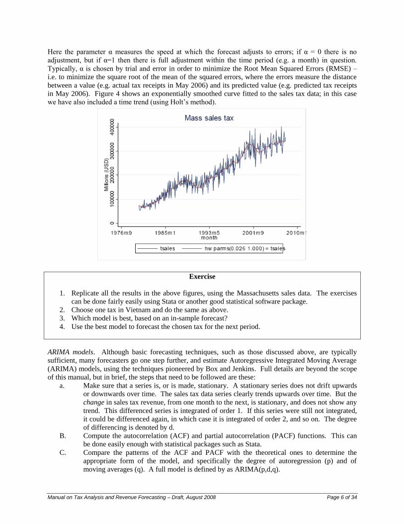
Here the parameter α measures the speed at which the forecast adjusts to errors; if α = 0 there is no
adjustment, but if α=1 then there is full adjustment within the time period (e.g. a month) in question.
Typically, α is chosen by trial and error in order to minimize the Root Mean Squared Errors (RMSE) –
i.e. to minimize the square root of the mean of the squared errors, where the errors measure the distance
between a value (e.g. actual tax receipts in May 2006) and its predicted value (e.g. predicted tax receipts
in May 2006). Figure 4 shows an exponentially smoothed curve fitted to the sales tax data; in this case
we have also included a time trend (using Holt’s method).
Exercise
1. Replicate all the results in the above figures, using the Massachusetts sales data. The exercises
can be done fairly easily using Stata or another good statistical software package.
2. Choose one tax in Vietnam and do the same as above.
3. Which model is best, based on an in-sample forecast?
4. Use the best model to forecast the chosen tax for the next period.
ARIMA models. Although basic forecasting techniques, such as those discussed above, are typically
sufficient, many forecasters go one step further, and estimate Autoregressive Integrated Moving Average
(ARIMA) models, using the techniques pioneered by Box and Jenkins. Full details are beyond the scope
of this manual, but in brief, the steps that need to be followed are these:
a. Make sure that a series is, or is made, stationary. A stationary series does not drift upwards
or downwards over time. The sales tax data series clearly trends upwards over time. But the
change in sales tax revenue, from one month to the next, is stationary, and does not show any
trend. This differenced series is integrated of order 1. If this series were still not integrated,
it could be differenced again, in which case it is integrated of order 2, and so on. The degree
of differencing is denoted by d.
B. Compute the autocorrelation (ACF) and partial autocorrelation (PACF) functions. This can
be done easily enough with statistical packages such as Stata.
C. Compare the patterns of the ACF and PACF with the theoretical ones to determine the
appropriate form of the model, and specifically the degree of autoregression (p) and of
moving averages (q). A full model is defined by as ARIMA(p,d,q).

Manual on Tax Analysis and Revenue Forecasting – Draft, August 2008 Page 7 of 34
D. Having determined p, d, and q, estimate the parameters of the model.
E. Use the model to generate forecasts.
In Stata, type help arima for the appropriate syntax. A typical command might look like arima tsales, arima(1,1,1)
Here is a fuller example:
With dynamic forecasting, we do not use the actual past values in order to make forecasts for the next
periods; instead we use the past estimated values. For recursive forecasting we forecast one period ahead
and then update our model using the newly-forecast values. Figure 5 shows the actual and predicted
values for the sales tax data, using dynamic forecasting and the ARIMA model whose results are shown
above:

Manual on Tax Analysis and Revenue Forecasting – Draft, August 2008 Page 8 of 34
Exercises
Repeat this exercise using data on one Vietnamese tax series.
Medium-Term Forecasting
Our purpose here is straightforward: forecast revenue for the next year or two.
a. The simplest practical approach (see Ribe p. xxx) is to assume that the revenue from a tax is, and
will continue to be, a constant fraction of GDP. Armed with a forecast of GDP, it is then
straightforward to forecast tax revenue.
Example. Let Rt refer to tax revenue in time t, and GDPt be Gross Domestic Product in time
t. Then we assume that (R/GDP)t = (R/GDP)t+i. For instance, revenue from a Value-Added
Tax (VAT) might be 8% of GDP. Now suppose that next year we expect GDP to rise by 2%
in real terms, and for inflation to be 7%. Then nominal GDP is expected to rise by 9.14% (=
(1+.02)*(1+.09)-1). So we can expect tax revenue to rise by 9.14% too.
Several things are required for this to be an adequate forecast.
First, the forecast of real GDP needs to be sound. Sometimes a Central Bank, or a reputable
magazine such as The Economist, may have forecasts; otherwise, one can buy forecasts from
companies that specialize in such things.
Second, the forecast of inflation should be plausible. In the year to July 2008 consumer price
inflation in Vietnam was 27 percent, the highest level in almost 15 years; but what inflation is it
reasonable to forecast for the coming year?
The third essential for this forecasting method is that revenue rises in line with GDP. In this case
we assume a tax buoyancy of 1. We define:
Tax buoyancy = % change in revenue / % change in tax base
where the tax base in this example is (or tracks) GDP. When measuring historical tax buoyancy
we simply compare actual tax revenues with actual GDP. For instance, suppose that GDP rose by
40% over the past decade and revenue rose by 36%, then the tax buoyancy would be 0.9 (=
36%/40%).
There is a distinction to be made between tax buoyancy and tax elasticity. We define:

Manual on Tax Analysis and Revenue Forecasting – Draft, August 2008 Page 9 of 34
Tax elasticity = % change in revenue / % change in tax base, holding the tax rules constant.
This measure is designed to quantify the effect of a change in the tax base on revenue, if no changes are
made to the tax code. For example, suppose that revenue in 2007 was 50 but rose to 60 this year; of this
increase, 8 was due to an increase in the tax rate (so revenue would only have risen to 52 if there were no
change in the tax code). Suppose that over the same period GDP rose by 3%. Then we have
Tax buoyancy = 6.7 (= 20%/3%)
Tax elasticity = 1.3 (= 4%/3%).
It is possible, and desirable, to refine this basic approach in a number of ways, to take account of different
tax bases, of changing tax rates, of disaggregation, of varying elasticities, and of inflation. Let’s deal with
these in turn.
b. One refinement to the basic approach is to use a tax base other than GDP. In this case one
projects the tax base, which could be consumption, or investment, or imports, for example, and
then links changes in tax revenue to changes in the tax base.
Example. Suppose that imports are expected to rise by 18% in domestic currency terms over
the coming year (which GDP is expected to rise by 12%), and suppose that we believe that
revenue from import duties rises in line with the value of imports. Then the expected
increase in tariff revenue is
18% = Tax buoyancy × forecast % rise in imports
= 1 × 18%.
Often we are obliged to use a proxy for the relevant tax base, rather than the “ideal” tax base, especially if
there is no reasonable forecast for the latter. For instance, the tax base for a cigarette tax is sales of
cigarettes. But suppose we do not have an independent forecast of cigarette sales. In that case we can use
some other magnitude in place of (“as a proxy for”) cigarette sales, such as total consumption
expenditures, or even GDP. G.P. Shukla recommends the following bases for taxes in Vietnam:
Some Taxes and their bases:
1. Taxes on income, profits GDP at factor cost (current & capital gains prices)
2. Estate duty GDP at factor cost (current prices)
3. Sales tax Private and government consumption (current prices)
4. Excises Private and government consumption (constant prices)
5. Taxes on specific services Private and government consumption (current prices)
6. Import duties Value/volume of imports
7. Stamp duties GDP at factor cost (current prices)
c. If our interest is in forecasting total tax revenue, how disaggregated should our calculations be?
Or should we simply use total tax revenue and relate it to, say, GDP? Generally the best solution
is to forecast, separately, each major tax – where “major tax” is defined as any tax that brings in
at least about 2% of total tax revenue – and for a residual category that includes all the minor
taxes. Too much disaggregation can lead to unstable results but too little disaggregation can lead
to imprecision.
To illustrate, consider the case of Hungary in 1988. Total government revenue was 790
billion forint, of which 697 came from tax revenue. The breakdown of the main sources of
revenue, and some suggested proxies for the tax bases, are shown in Table xxx.

Manual on Tax Analysis and Revenue Forecasting – Draft, August 2008 Page 10 of 34
Table xxx. Disaggregation and Proxies for Tax Bases, Hungary, 1988
Tax Revenue
(bn ft)
% of total gov.
revenue
Model
separately?
Proxy for base
Personal income tax 5 1 No
Corporation income tax 119 15 Yes GDP at factor cost
Social security tax 194 25 Yes GDP at factor cost;
or wages and
salaries
Property tax 1 <1 No
Turnover tax 128 16 Yes Private consumption
Excise taxes 80 10 Yes Private consumption
Other taxes on goods & services 94 12 Yes Private consumption
Imports 36 5 Yes Value of imports
Poll taxes 3 <1 No
Other taxes 37 5 Maybe GDP at factor cost
Non-tax revenue 93 12 Yes GDP at factor cost
d. The next refinement to the model is to use revenue elasticities (ε) other than 1. But what
revenue elasticities are appropriate? We might make the following generalizations:
ε = 1 if a tax is proportional, there are few collection lags, and it is computed on an ad valorem
basis. A good example is the VAT.
ε <1 if there are long collection lags (so that the purchasing power of the collections lags behind
the base), the tax is collected on a specific basis (e.g. so many cents per liter of gasoline) and
there is inflation, there are caps on the base (e.g. US social security insurance, where the tax is
only levied up to a certain income limit), and where there are administrative and compliance
problems. Good examples include property and land taxes, and most excise taxes.
ε >1 if there is a progressive rate structure, of if there is inflation and the tax brackets are not
indexed. The classic example here is a progressive personal income tax.
At this point we need to make a distinction between nominal and real values. Suppose GDP rises by 8%
between one year and the next; in general, part of the increase reflects a rise in the quantity of goods and
services produced (real GDP growth) and the rest reflects increases in prices. In this example, if inflation
is 5%, then real GDP growth is about 3%.2
The issue now arises of whether to forecast real, or nominal, tax revenue? In large measure the issue
comes down to whether it is better to use real or nominal tax elasticities.
To illustrate, suppose nominal GDP rises from $200 to $250 between 2007 and 2008, which is an
increase of 25%. And suppose that over the same period, tax revenue rose from $40 to $48, and
prices rose by 15%, and than no changes were made in the tax system. Then we have:
Nominal tax buoyancy (= elasticity here, given no tax changes) = 20%/25% = 0.8.
But if we first strip out inflation, to get real growth rates, we have:
Real tax buoyancy (= elasticity here) = 4.35% / 8.70% = 0.5.
2 Let П
e be expected inflation, r be the growth rate of real GDP, and g be the growth rate of nominal GDP. Then we
have (1+g) = (1+r) × (1+Пe). For modest increases, g ≈ r + П
e.

Manual on Tax Analysis and Revenue Forecasting – Draft, August 2008 Page 11 of 34
For the real increase in tax revenue we have (1 + 20%) / (1 + 15%) – 1, and for the real increase
in GDP we have (1 + 25%)/(1 + 15%) – 1.
Here there are two options for forecasting. We could take a forecast of real GDP growth, apply the real
tax elasticity, and then add an adjustment for inflation (assuming that an extra percentage point of
inflation leads to an extra percentage point of revenue). Or we could take a forecast of nominal GDP
growth, and use the nominal tax elasticity.
Following up on the previous example, suppose we believe that GDP will grow by 4% in the year
ahead, and that inflation will be 10%, which means that we expect nominal GDP to rise by
14.4%. Then our forecasts of tax revenue may be made as follows:
Using the nominal tax elasticity: % change in tax revenue = 0.8 × 14.4% = 11.52, so new
tax revenue is $53.53.
Using real tax elasticity: % change in real tax revenue = (0.5 × 4%) = 2%. New real tax
revenue is therefore $48.96. Inflate this by 10% inflation to get the nominal tax revenue
of $53.86.
Note that the outcomes are not the same. By applying the nominal tax elasticity we are implicitly
assuming that it applies equally to real increases in GDP and to inflationary increases in GDP.
By using the real tax elasticity, we implicitly apply a tax elasticity of 1 on the inflationary
component of GDP increases.
As a general proposition, it is usually better to apply real (rather than nominal) tax elasticities. How, then,
are they to be computed?
A popular method is to use historical data on changes in the base and in revenue. First deflate the two
series to put then in real terms; a regression of the log of real tax revenue on real GDP (or whatever the
base is) will then yield a measure of tax buoyancy.
Example. Here is some (hypothetical) information on the evolution of tax revenue and GDP
over the past several years. The real series are obtained by deflating the nominal series by the
consumer price index.
Tax buoyancy series
Year
2000 2001 2002 2003 2004 2005 2006 2007
Tax revenue, nominal 240 283 315 339 361 442 520 568
GDP, nominal 1,200 1,348 1,486 1,654 1,755 2,027 2,418 2,665
Inflation, % p.a. 0.07 0.06 0.065 0.04 0.09 0.12 0.07
So:
tax revenue, real 240 265 278 281 288 323 339 346
GDP, real 1200 1,260 1,310 1,369 1,397 1,481 1,577 1,624
A regression of the log of real tax revenue on the log of real GDP gives the results shown here,
with a buoyancy of 1.183. Also shown are the results of a regression of the log of nominal tax
revenue on nominal GDP, which shows a value of 1.069. Inflation tends to push up GDP and tax
revenue, in nominal terms, at the same time, forcing the value of the coefficient (i.e. the measure
of buoyancy) towards 1.

Manual on Tax Analysis and Revenue Forecasting – Draft, August 2008 Page 12 of 34
Coef. SE t P>t95% confid. Interval
ltaxreal
lgdpreal 1.183 0.079 15.060 0.000 0.991 1.375
_cons -2.886 0.569 -5.070 0.002 -4.278 -1.494
ltaxnom
lgdpnom 1.069 0.030 35.170 0.000 0.994 1.143
_cons -2.074 0.227 -9.130 0.000 -2.630 -1.518
As an exercise, use the information on nominal GDP and tax revenue, and inflation, to (i)
construct the series of real tax revenue and real GDP, and (ii) recreate the regression results
shown here.
Once we have a measure of the tax elasticity (ε), we can measure the proportionate change in revenue as
%ΔR = ε × %Δbase.
For example, if the elasticity of excise taxes with respect to consumption spending is 0.85, and
consumption spending is forecast to rise by 7.1%, then expect excise tax revenue to rise by 6.0% (= 0.85
× 7.1%).
Exercise 1: Basic Revenue Projections
1. The numbers given in the table break down government tax revenue for Kenya into its main components.
Calculate the tax buoyancy for each of the taxes listed,
a. First using the data in current prices, and
b. Then using the data in constant prices.
c. What do you find most interesting in these results?
d. Why have you ended up measuring tax buoyancy in a. and b., and not tax elasticity?
1986 1987 1988 1989 1990
GDP, 1990 Ksh, m 7,135 7,482 7,870 8,260 8,634
GDP, nominal, Ksh, m 5,115 5,648 6,472 7,426 8,634
GDP deflator 146.22 153.96 167.73 183.36 203.95
Tax revenue (Ksh, m)
Income tax 386 454 512 599 710
VAT on domestic goods 242 301 351 324 435
VAT on imports 156 219 237 317 348
Import duty 247 274 300 348 314
Excises 106 123 137 149 182
Other taxes 104 82 106 94 109
TOTAL TAX REVENUE 1,241 1,453 1,644 1,831 2,098
2. Assume that for 1991, real GDP will rise by (i) 4%, (ii) 5%, (iii) 6%. Use the information from question 1
to develop six different projections of real tax revenue for each of the major tax categories for 1991, using
a. The tax buoyancy figures for 1989-90.
b. A tax buoyancy of 1.
c. Which projection do you favor?
d. If you wanted to make your projections more accurate, what information would you want? Do you
expect that such information is readily available?

Manual on Tax Analysis and Revenue Forecasting – Draft, August 2008 Page 13 of 34
e. A serious problem that arises when trying to estimate tax elasticity – as opposed to tax
buoyancy – using historical data is that we need to take into account the effects of any
significant changes in the tax code that might have occurred over time. The idea here is
first to generate a “clean” series of revenue that is purged of the effects of discretionary
changes in the tax code.
The most practical method is that of proportional adjustment; if we have an estimate of the revenue
effects of a discretionary change, we can then adjust the series proportionately. This is most easily seen
with an example. Suppose that corporate income tax revenue for Hungary, in billions of forint, was as
shown Table xxx, and that discretionary changes in the tax laws are believed to have added 8 to revenue
in 1983 and 15 in 1987, but to have reduced revenue in 1985 by 12. We can then construct a clean series
that shows what revenue we could reasonably have expected to get if the 1988 tax code were in effect
throughout the period.
1 B C D E F G H I J
2 1981 1982 1983 1984 1985 1986 1987 1988
3 Actual CIT revenue, bn forint 77 70 86 94 70 98 117 124
4 Discretionary changes 8 -12 15
5 Tax code rate, as % of 1988 93 93 102 102 87 87 100 100
6 So clean tax series (1988 rates) 83.1 75.6 84.2 92.0 80.3 112.4 117.0 124.0
=(1-E3/E4)*E5 =($J5/G5)*G3
It is sometimes possible to create a clean series of revenue numbers by applying the current tax structure
to the past, recalculating past revenue as it would have been if the current tax regime were in place back
then. In practice this is rarely done, since it requires substantial information about the tax base in the past;
for example, consider the challenge involved in applying today’s income tax rates to the incomes of
actual and potential taxpayers in other years.
If tax changes are relatively rare, it is sometimes possible to deal with the problem that such changes pose
to the measurement of tax elasticity by including the appropriate dummy variables in the regression
equation that is being estimated. For example, suppose that changes in excise tax rates came into effect in
2003, but were stable otherwise. Our interest is in estimating the tax elasticity for excise taxes. Consider
a regression of this form:
Ln(Revenue from excises) = a0 + a1 ln(consumer spending) + a2 D
where D is a dummy variable that is set to 1 for the years 2003 and after, and to 0 otherwise. This
regression line shifts up in 2003, but the fundamental relationship between proportionate changes in
consumer spending, and proportionate changes in excise tax revenue, will still be given by a1. This is
now a tax elasticity, not a tax buoyancy, because the effect of discretionary changes in the tax code have
been controlled for by using the dummy variable.

Manual on Tax Analysis and Revenue Forecasting – Draft, August 2008 Page 14 of 34
Tax policy analysis
The purpose of tax policy analysis is to predict the effects of changes in tax rates, bases, exemptions,
deductions, and other reforms to the tax code. Most analysis is based on tax calculator models.
Model 1. Tax calculator model based on a sample of current taxpayers.
Data needed: A sample of tax returns, including all the relevant data (income, tax paid, etc.) that are
available. This is available for personal income tax in Vietnam, for 2004, and includes
data on foreigners.
How? Change tax rates and/or bases, and re-calculate the amount that each of the sampled
taxpayers would have to pay. Gross up to get overall effect.
How useful? Satisfactory, if (i) data are sound, (ii) information on the sampling procedures is
available, and (ii) the changes that are envisaged would not lower the threshold for
paying tax (because only high-income individuals are included in such a sample). Allows
one to measure revenue effects, but not incidence.
Model 2. Tax calculator model based on household survey data.
Data needed: Data from a household survey that has information both on income and spending for each
household. Data from the Vietnam Household Living Standards Survey of 2006 should
be available sometime in February 2008.
How? Change tax rates and/or bases, and use these to re-compute the amount of tax that each
household can be expected to pay. Gross up to get the overall effect.
How useful? A powerful tool that allows one to measure both revenue and incidence effects of tax
changes. Can be part of an integrated tax calculator that allows one to change several
taxes simultaneously and trace the net effects on revenue and incidence. For the personal
income tax in Vietnam, useful if one is considering lowering the threshold at which one
pays taxes, but of limited value for measuring other changes in the personal income tax,
given the small sample size.
Model 3. Tax calculator model based on disaggregated macroeconomic data
Data needed: For an analysis of changes in the coverage of the Value-Added Tax (VAT), an input-
output table; for trade taxes, a detailed breakdown of imports and associated tariff rates
and revenue by harmonized system (or other) category.
How? Change the tax rates and/or base and recomputed expected revenue.
How useful? Unless the input-output table is very detailed, changes in the VAT are typically more
accurate when applied to household survey data. However, this is the only approach that
will allow one to estimate the effect of changes in the structure or coverage of taxes on
trade. Allows one to measure revenue effects, but not incidence.
G.P. Shukla explains how he constructed a tax calculator model for the Vietnamese corporation income
tax as follows:
“Steps to construct the model:
1. Sampling of tax returns. Stratified sampling is suggested. First, different strata are established on
the basis of some critical categories such as size of assets, income, industry, or region. Firms in
each stratum resemble by the category used to select the strata. Second, sample of firms will be
selected from these strata. Different weights are assigned to each stratum, and will be used to
determine the proportion of firms in each stratum to be randomly drawn for the ultimate sample.

Manual on Tax Analysis and Revenue Forecasting – Draft, August 2008 Page 15 of 34
For example, if strata are selected on the basis of gross income, higher income strata will be given
higher weights; the proportion of firms drawn from those strata will be higher. Also, note that
samples from different filing periods may also be selected to account for non-calendar filing and
filing extensions. The “tax return” sheet has embedded a weight column that could be adjusted
with the proportion of firms represented by each stratum.
2. Data cleaning. This step is to ensure consistency and reliability of data selected for the
simulations.
3. Data completion process. Filling in missing data relies on either data from corporate financial
statements, and/or imputation data.
4. Construct a tax calculator to simulate corporate income tax. Corporate income tax base is derived
from gross income from different sources minus itemized deductions including costs of goods
sold, depreciation allowance, interest payments, overheads expenses, and any net operating loss
from prior years. Tax payable is estimated as the product of tax base and corporate income tax
rate. Tax liability should also be adjusted for any tax credits that are allowed. From this base tax
calculator, impact of any proposed changes in the corporate income tax code on a representative
firm and on government tax revenue will then be simulated.
Results:
Using the 91 CIT individual tax return data base available, a policy analysis scenario was constructed
using a 23% CIT flat rate across the different corporations organization types. After performing the tax
calculator model, it is expected that the government would collect VND 86,917 million, from VND
71,159 million estimated with the current CIT structure, which represents an additional CIT collection of
VND 15,758 million, or 22.1%.”
Exercise 3: Revenue Estimation – One Good These questions provide practice with computing and using elasticities. Some are quite quick and easy (but others
are not!).
1. The price of a can of Coke is VND12,000. Assume that VND2,000 of this represents tax. Now the tax
is increased by 50% to VND3,000, and all of this increase is passed on to consumers. If the price
elasticity of demand is -2:
a. By what proportion will the quantity of Coke demanded fall?
b. By what proportion will tax revenue rise?
2. Tourists buy lots of lacquer boxes. Assume that the supply is horizontal, and the average price of a
box (before tax) is VND40,000.
a. If the demand curve is given by Qd = 18000 – 0.25P, draw the demand and supply curves, and
calculate the quantity of boxes sold.
b. Introduce a VAT of 10 percent. Show and calculate the effect this will have on
i. The selling price;
ii. The quantity sold;
iii. Tax revenue; and
iv. Excess burden.
c. Redo b. using a VAT of 15 percent. How much extra excess burden is created, per dong of extra
revenue, when the VAT is increased?

Manual on Tax Analysis and Revenue Forecasting – Draft, August 2008 Page 16 of 34
3. Based on your answers to 2.b and 2.c, which of the following assertions is true?
a. When the tax rate rises, the excess burden rises proportionately faster than tax revenue.
b. When the tax rate rises, the price paid by consumers rises faster than tax revenue.
c. When the tax rate rises, tax revenue will always rise.
d. We have, when supply is horizontal:
Revenue = R = tP0Q0 + t2P0Q0η, Excess burden = EB = – (1/2) t
2P0Q0η.
These formulae are approximate. Use them to calculate the approximate values of tax revenue and
excess burden when the VAT is raised from 0% to 10%. [Hint: you will need to calculate at the
pre-tax equilibrium first.] The reason that these formulae are so useful is that in practice we rarely
have an equation for the demand curve, but we are likely to have at least an approximate value for
the demand elasticity.
e. Someone proposes that small enterprises, with an annual turnover of less than VND50 million, be
exempt from paying VAT on their sales. What will happen to the structure of the market for
lacquer boxes if a VAT is imposed, knowing that this exemption is in effect?
4. This table provides information on the output of coffee in Kenya, along with the price received by
coffee farmers (the “farmgate” price) and the consumer price index.
a. Recalculate the farmgate prices in 1990 shillings. This gives the “real” price of coffee.
b. Plot the real price of coffee (on the vertical axis) against the quantity produced (horizontal axis).
A line through these points gives the supply curve for coffee, and could be estimated using
regression. Do this.
c. Estimate the elasticity of supply (i.e. ε). This could be done by calculation %ΔQ/ΔP for each year
(e.g. between 1986 and 1987, etc.), and then taking the mean of your results. Or try regressing the
log of output (Q) against the log of price (P); the coefficient on P gives the elasticity.
d. Why do we believe that our results give a supply, and not a demand, elasticity?
1986 1987 1988 1989 1990
Consumer price index 354.6 379.5 420.0 464.4 523.0
Coffee
Price (Ksh/kg) 50.20 36.62 44.65 43.12 36.36
Quantity produced (‘000 tonnes) 113.9 104.3 128.7 116.9 103.9
5. Using the data in the table below
a. Calculate the price elasticity of demand for gasoline in Kenya.
b. Suppose that a tax of Ksh 1/liter were introduced in 1990. Compute tax revenue and gasoline
sales. [Note: Assume there are 1,200 liters of gasoline per tonne.]
Price of
gasoline
Sales of
gasoline
Price of
diesel fuel
Population GDP,
nominal
GDP deflator
Ksh/liter ‘000 tonnes Ksh/liter Millions Kpounds, m
1979 2031 0.742
1980 4.39 300.8 3.06 15.84 2298 0.813
1981 5.98 298.5 4.23 16.36 2668 0.895
1982 7.06 269.3 5.20 16.91 3078 1.000
1983 7.52 256.4 5.48 17.48 3452 1.105
1984 7.94 257.7 5.79 18.06 3852 1.224
1985 8.13 267.8 5.94 18.66 4375 1.325
1986 7.74 295.1 5.47 19.29 5115 1.462
1987 8.16 321.8 5.54 19.93 5648 1.540
1988 8.54 325.0 5.67 20.60 6472 1.677
1999 9.03 376.7 5.99 21.28 7426 1.834
2000 11.70 339.9 8.55 22.01 8634 2.039
6. Estimate the price elasticity of demand for gasoline in Vietnam (!). [NB. The real challenge here is in
finding the data – a very common problem in research.]

Manual on Tax Analysis and Revenue Forecasting – Draft, August 2008 Page 17 of 34
Tax Incidence
When considering changes to the tax code, policy makers want to know who will gain and who will lose.
This is done by measuring the incidence of a tax.
It is important to distinguish between statutory (or nominal) incidence and effective incidence. Statutory
incidence tells us who, legally, must pay the tax, while effective incidence indicates who really bears the
burden of the tax. For example, a supermarket may have to collect VAT on its sales and send the tax
revenue to the treasury (statutory incidence), but the real burden of the tax may be borne by consumers
who have to pay higher prices when the VAT is introduced.
It is not always easy to figure out who bears the incidence of a tax, but a demand and supply diagram
helps clarify the situation. Starting with the original demand and supply curves, we have quantity Q0 and
price P0. Now introduce a tax on this good. We may think of this as pushing up the cost of supplying the
good to consumers, shifting the supply curve up to the “Supply + Tax” curve. The new price faced by
consumers is P1d, but part of this represents tax, so suppliers only get P1s. In this example, the burden of
the tax is shared between consumers (who pay more and lose the striped area) and producers (who receive
less and lose the dotted area).
If the supply curve is horizontal, which is plausible for many manufactured goods, then the tax is entirely
shifted onto consumers. Here, then, are the most common assumptions that are made about the effective
incidence of some of the more important taxes:
a. VAT. Falls on consumers.
b. Excise taxes. Fall on consumers.
c. Personal income tax. Falls on employees.
Quantity
Price
Demand
Supply + Tax
Supply P1d
P0
Q1 Q0
P1s

Manual on Tax Analysis and Revenue Forecasting – Draft, August 2008 Page 18 of 34
d. Tariffs. Fall on consumers, either directly (if on final goods) or indirectly (if on intermediate
goods).
e. Export taxes. Fall on domestic producers (who still get the world price, but now face a tax).
f. Corporation income tax. Controversial. In an open economy with perfectly mobile capital, it
falls on labor and perhaps consumers, because capital can insist on getting the same return (or
it will move abroad) and so passes on the tax in the form of lower wages or higher prices. On
the other hand, capital is not perfectly internationally mobile, and so bears part of this tax.
The extent to which this tax is borne by capital is still a subject of research.
g. Property tax. xxx
To measure tax incidence, one needs detailed information on households, and this typically comes from
surveys of households. In Vietnam, there have been five major living standards measurement surveys,
and such surveys have been done in many other countries. In some cases the major household surveys
focus on measuring expenditures, mainly as an input into constructing consumer price indices.
Given assumptions about incidence, and household data, the procedures to be followed in order to
measure incidence are relatively simple (in principle at least!), as follows:
1. Measure household income and/or expenditure; typically this is shown in per capita terms.
2. Apply the taxes, or changes in taxes, to household spending and/or income, given the
assumptions about incidence.
a. Example 1: If the tobacco excise tax is raised from $1 to $2 per pack, and we assume the
burden of this tax falls on consumers, then compute how much extra households would
spend on cigarettes as a result of the tax increase.
b. Example 2: If the top personal income tax rate is raised from 35% to 38%, calculate how
much tax households would spend (i) under the old tax system, and (ii) under the new tax
system.
3. Incorporate any required behavioral changes.
a. Example 1: If the tobacco excise tax is raised from $1 to $2 per pack, the higher price
will deter some buyers. One could apply an appropriate demand elasticity to determine
by how much consumers will cut back. So if the selling price rises from $4 to $5 per
pack as a result of the tax increase, and the own-price elasticity of demand is -0.2, then
the quantity will fall by 5%j.
b. Example 2: If the top personal income tax is raised form 35% to 38%, we might expect
more tax evasion; perhaps reported income will be understated by a further 1%. Again,
we can factor this into the computation of revenue and incidence (although this is
sometimes difficult, and we generally lack viable information on evasion).
4. Present and summarize the results effectively.
Here is an example, from a tax calculator model of the Vietnamese tax system, of how the results might
be presented. This particular case shows the effects of the introduction of a 1% tax on property (levied on
the value of residential property over VND100 million per household). The first block of numbers
divides the population into ten deciles, from poorest to richest, as measured by expenditure per capita. It
shows the estimated expenditure per capita of each decile in 2009 and the tax that they would expect to
pay under current tax rules. Then the residential property tax is introduced, and the burden of the tax is
allocated in line with the amount of tax that each household would have to pay – using information from
the 2006 Vietnam Household Living Standards Survey, which asked people about the value of their
residential property. This tax would be highly progressive, hitting richer households proportionately
much more severely than poor households, as the results in the final column show.
The second block of numbers shows the effects of the tax for each of Vietnam’s eight regions; here we
see that the property tax would have an especially large effect in the Southeast (centered on Ho Chi Minh

Manual on Tax Analysis and Revenue Forecasting – Draft, August 2008 Page 19 of 34
City) and the Red River Delta (centered on Hanoi). The third panel breaks down the tax by urban vs.
rural residence; this is a tax that would mainly tax townspeople.
Distributional Expenditure/cap Est. tax/capita Est. tax/expenditure Simulated tax/capita Simul. Tax/expend Change due to % change due to
Results of the simulation 2009 2009 2009 2009 2009 new tax regime new tax regime
Expenditure per capita deciles 1 (poorest) 3,553 279 7.9% 282 7.9% 2 0.9%
2 5,219 454 8.7% 460 8.8% 6 1.4%
3 6,466 668 10.3% 689 10.7% 21 3.0%
4 7,682 825 10.7% 903 11.8% 78 8.7%
5 9,019 1,009 11.2% 1,119 12.4% 110 9.9%
6 10,626 1,272 12.0% 1,467 13.8% 195 13.3%
7 12,700 1,774 14.0% 2,124 16.7% 350 16.5%
8 15,652 2,060 13.2% 2,655 17.0% 595 22.4%
9 20,595 3,002 14.6% 4,419 21.5% 1,417 32.1%
10 (richest) 40,293 5,404 13.4% 10,159 25.2% 4,755 46.8%
Regions 1: Red River Delta 14,640 1,647 11.3% 2,713 18.5% 1,065 39.3%
2: Northeast 10,254 1,067 10.4% 1,373 13.4% 307 22.3%
3: Northwest 7,804 881 11.3% 1,131 14.5% 250 22.1%
4: North Central Coast 8,977 1,040 11.6% 1,252 13.9% 212 17.0%
5: South Central Coast 12,020 2,261 18.8% 2,684 22.3% 423 15.8%
6: Central Highlands 10,580 1,447 13.7% 1,785 16.9% 338 19.0%
7: Southeast 21,054 2,587 12.3% 4,762 22.6% 2,175 45.7%
8: Mekong Delta 11,899 1,689 14.2% 1,930 16.2% 241 12.5%
Areas Urban 22,018 2,973 13.5% 5,125 23.3% 2,152 42.0%
Rural 9,952 1,200 12.1% 1,442 14.5% 242 16.8%
Vietnam overall Average 13,176 1,675 12.7% 2,428 18.4% 753 31.0%
Gini coefficient 0.390 0.461
A fuller description of the Vietnam tax calculator model is given in the appendix.
Exercise 4 provides some practice with a tax calculator model. It is based on information from a survey,
undertaken in 2005 by the General Department of Taxation, of “high income individuals”. All of these
individuals were paying personal income tax, or household business tax, in that year. Originally the
survey was designed to sample 15,500 individuals, chosen from among the approximately 300,000 people
on the tax rolls at that time, of which 3,200 were foreigners, 7,200 were Vietnamese paying the personal
income tax, and 5,100 were Vietnamese paying the household business income tax. The response rate
was 74%, so there were 11,532 usable replies, although the response rate was lower among foreigners,
and in Ho Chi Minh City.
When using survey data it is essential first to ask about the validity of the data. The quality of
information from this questionnaire is not especially high; the questionnaire was rather short, and the
surveying was done by tax agents, which many have led to strategic answering by respondents. On the
other hand, this is the only available survey that has any information about the income and spending
habits of foreigners working in Vietnam.
To fix ideas, Table xxx provides some basic data on income from the survey of high-income individuals.
Of note are the high average wages of foreigners, and the low levels of reported expenditures for all
groups of households.
Table xxx. Income and Estimated Tax for High-Income Households, 2005
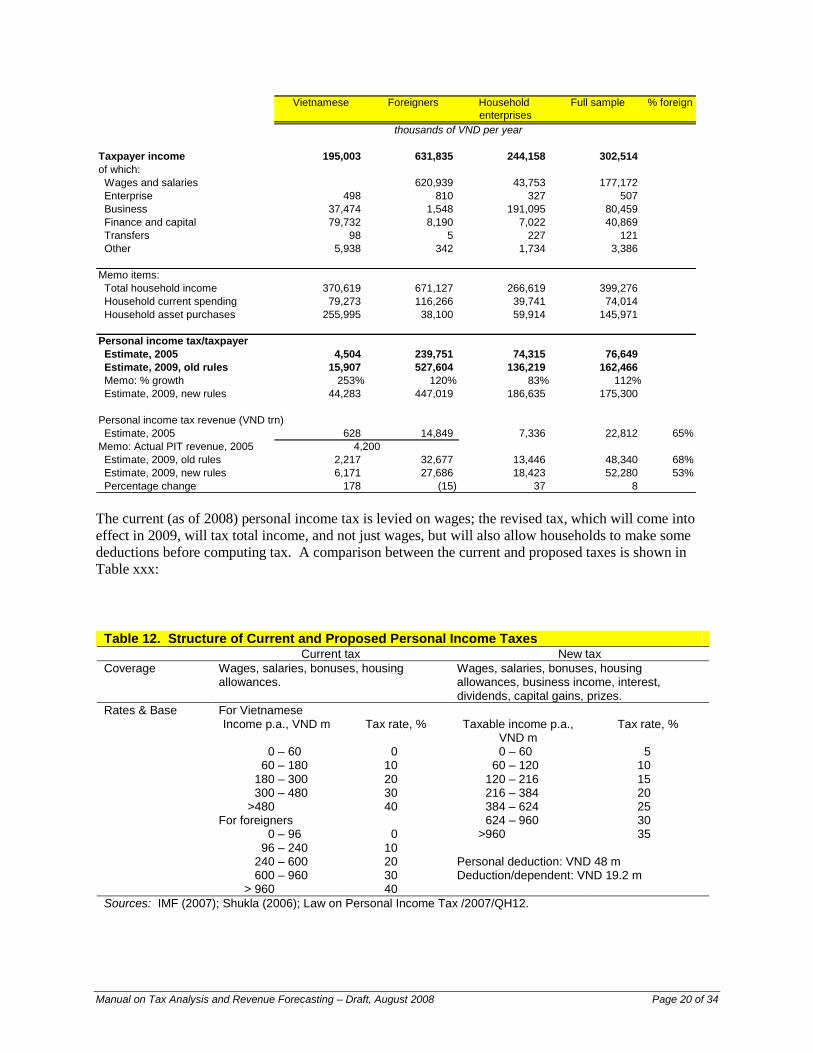
Manual on Tax Analysis and Revenue Forecasting – Draft, August 2008 Page 20 of 34
Vietnamese Foreigners Household Full sample % foreign
enterprises
Taxpayer income 195,003 631,835 244,158 302,514
of which:
Wages and salaries 620,939 43,753 177,172
Enterprise 498 810 327 507
Business 37,474 1,548 191,095 80,459
Finance and capital 79,732 8,190 7,022 40,869
Transfers 98 5 227 121
Other 5,938 342 1,734 3,386
Memo items:
Total household income 370,619 671,127 266,619 399,276
Household current spending 79,273 116,266 39,741 74,014
Household asset purchases 255,995 38,100 59,914 145,971
Personal income tax/taxpayer
Estimate, 2005 4,504 239,751 74,315 76,649
Estimate, 2009, old rules 15,907 527,604 136,219 162,466
Memo: % growth 253% 120% 83% 112%
Estimate, 2009, new rules 44,283 447,019 186,635 175,300
Personal income tax revenue (VND trn)
Estimate, 2005 628 14,849 7,336 22,812 65%
Memo: Actual PIT revenue, 2005
Estimate, 2009, old rules 2,217 32,677 13,446 48,340 68%
Estimate, 2009, new rules 6,171 27,686 18,423 52,280 53%
Percentage change 178 (15) 37 8
thousands of VND per year
4,200
The current (as of 2008) personal income tax is levied on wages; the revised tax, which will come into
effect in 2009, will tax total income, and not just wages, but will also allow households to make some
deductions before computing tax. A comparison between the current and proposed taxes is shown in
Table xxx:
Table 12. Structure of Current and Proposed Personal Income Taxes Current tax New tax
Coverage Wages, salaries, bonuses, housing allowances.
Wages, salaries, bonuses, housing allowances, business income, interest, dividends, capital gains, prizes.
Rates & Base For Vietnamese Income p.a., VND m Tax rate, % Taxable income p.a.,
VND m Tax rate, %
0 – 60 0 0 – 60 5 60 – 180 10 60 – 120 10 180 – 300 20 120 – 216 15 300 – 480 30 216 – 384 20 >480 40 384 – 624 25 For foreigners 624 – 960 30 0 – 96 0 >960 35 96 – 240 10 240 – 600 20 Personal deduction: VND 48 m 600 – 960 30 Deduction/dependent: VND 19.2 m > 960 40
Sources: IMF (2007); Shukla (2006); Law on Personal Income Tax /2007/QH12.

Manual on Tax Analysis and Revenue Forecasting – Draft, August 2008 Page 21 of 34
Exercise 4: Personal Income Tax – Calculator Model
All these questions use the actual data from the 2005 survey of high-income taxpayers.
7. Load the data file (hiincsurvey1.dta) and become familiar with the variables. Start a log file, to keep
your workings. Summarize the data. Identify at least one surprising or unexpected feature of the
numbers.
8. The attached *.do file (HiinctaxcalcMay27.do) performs the basic set of calculations. Execute this file
a few lines at a time, in order to understand what it does. Are there any discrepancies between the
results shown here and those in the table entitled “Income and Estimated Tax for High-Income
Households, 2005”?
9. Now, some real analysis.
a. How robust are the results to the assumptions made about inflation and economic growth? To
check this, re-do the analysis assuming
i. Inflation of 15% in 2008 and 12% in 2009.
ii. GDP growth of 7% in 2008 and 7% in 2009.
b. You have been asked to estimate the revenue effects of a number of different possible changes in
the personal income tax (other than the ones set out in Table 12). Do this for each of the
following:
i. The new tax rates would be Taxable inc. VND m 0- 60- 120- 216- 384- 624- 960-
Tax rate, % 0 5 10 15 20 25 30
ii. The new tax rates would be Taxable inc. VND m 0- 60- 120- 216- 384- 624- 960-
Tax rate, % 0 10 10 20 20 30 30
iii. The new tax rates would be Taxable inc. VND m 0- 60- 120- 216- 384- 624- 960-
Tax rate, % 20 20 20 20 20 20 20
iv. The tax rates would be as in Table 12, but
1. Personal deduction of VND3m/month, Dependent deduction of VND1.5m/mth
2. Personal deduction of VND4m/month, Dependent deduction of VND1.6m/mth
3. Personal deduction of VND5m/month, Dependent deduction of VND2m/mth
4. Personal deduction of VND6m/month, Dependent deduction of VND2.5m/mth
5. Personal deduction of VND8m/month, Dependent deduction of VND3m/mth
v. Every individual would get the same deduction per person, which would be
1. VND4m per month
2. VND6m per month
vi. The tax rates would be as in Table 12, but the brackets would be
1. Twice as wide
2. Like the current brackets for Vietnamese
3. Like the current brackets for foreigners
4. As in Table 12, but adjusted for the inflation of 2008 and 2009.
10. Now
a. Create a table summarizing your results, in a way that is easy to read and understand. [It’s OK to
do this in Vietnamese, if you prefer.]
b. Which of the many variants that you have considered do you prefer? Why?

Manual on Tax Analysis and Revenue Forecasting – Draft, August 2008 Page 22 of 34
Exercise 5: Tax Incidence This exercise asks you to measure the incidence of taxes in Vietnam, using the JHindirtaxmasterMay21.do file.
Once it is running correctly, it can then be modified to examine the incidence of changes in taxes.
1. Load the relevant data files into a directory called C:\stata9\vlss06.
2. Modify JHindirtaxmasterMay21.do so that it reads these files.
3. Run JHindirtaxmasterMay21.do in small bits, in order to understand how it works.
4. Open a log file called taxrun1.log and then run JHindirtaxmasterMay21.do in its entirety. Close the
log file.
5. Now create a *.do file called JHindirtaxmasterMay29.do in which VAT is charged on food. Open a
new log file called taxrun2.log and then run JHindirtaxmasterMay29.do in its entirety.
6. Compare the results of 4. with those in 5, by creating a table that looks like Table 7 in Taxation in
Vietnam: Who Pays What? (reproduced below).
7. Compute Gini and concentration coefficients for the taxes in 6. using GiniMar2008.do .
Table 7. Tax Paid by Vietnamese Households in 2006, by Expenditure per capita Deciles Table xxx. Tax paid by Vietnamese households in 2006, by expenditure per capita quintile
1 (poor) 2 3 4 5 6 7 8 9 10 (rich) All % hh
paying
Household expenditure per capita 2,000 2,938 3,640 4,324 5,077 5,981 7,149 8,811 11,593 22,681 7,417
Total tax paid 156 252 372 458 557 709 984 1,151 1,679 3,146 946 100.0
of which:
value-added tax 90 144 212 263 319 420 525 662 1,007 1,577 522 100.0
excise taxes 13 23 30 38 47 60 73 93 141 333 85 97.3
educational fees 22 37 58 73 88 112 130 168 191 264 114 62.1
agricultural fees 12 22 31 37 33 34 28 28 23 12 26 40.2
other fees 16 22 29 34 41 48 65 83 133 247 72 99.0
taxes on household enterprises 3 3 12 12 30 35 163 116 184 651 121 15.4
personal income tax - - - - - - - - 1 61 6 0.2
Total tax paid 7.8 8.6 10.2 10.6 11.0 11.9 13.8 13.1 14.5 13.9 13.4
of which:
value-added tax 4.5 4.9 5.8 6.1 6.3 7.0 7.3 7.5 8.7 7.0 7.0
excise taxes 0.6 0.8 0.8 0.9 0.9 1.0 1.0 1.1 1.2 1.5 1.1
educational fees 1.1 1.3 1.6 1.7 1.7 1.9 1.8 1.9 1.6 1.2 1.5
agricultural fees 0.6 0.8 0.9 0.9 0.7 0.6 0.4 0.3 0.2 0.1 0.4
other fees 0.8 0.8 0.8 0.8 0.8 0.8 0.9 0.9 1.1 1.1 1.0
taxes on household enterprises 0.1 0.1 0.3 0.3 0.6 0.6 2.3 1.3 1.6 2.9 1.6
personal income tax - - - - - - - - 0.0 0.3 0.1
Expenditure per capita deciles
thousands of VND p.a.
as percentage of expenditure
Notes. Revenue from value-added tax, excise taxes, and personal income tax, are estimated based on spending and income patterns. Results are
preliminary, and based on the VHLSS survey of 2006. All figures are in prices of 2006.

Manual on Tax Analysis and Revenue Forecasting – Draft, August 2008 Page 23 of 34
Appendix 1
Vietnam Tax Calculator Model
Jonathan Haughton
August 7, 2008
Introduction
It is useful to be able to estimate the revenue and distributional effects of changes in the structure of taxes,
especially when considering possible alterations to the tax code.
The Vietnam Tax Calculator Model (VtaxModel) allows one to undertake such policy simulations quickly
and conveniently. The user specifies the desired changes in tax rates or brackets, and the model computes
the effects on tax revenue, as well as measuring the change in the burden of taxes across expenditure
deciles, across regions, and between urban and rural households. In some cases the user may also adjust
the elasticities of demand that are assumed to apply.
For a discussion of the structure of the Vietnamese tax code, and some simulation results, see Haughton
(2008), which is worth reading, or at least skimming, before using the VtaxModel. The results in that
paper differ slightly from those generated by the VtaxModel; the latter continues to evolve, but may be
considered to be more up to date and reliable.
The VtaxModel works well, but there may still be some glitches. Please do not hesitate to get in touch
([email protected] ) if any problems arise, so that they may be resolved as quickly as possible.
All the results refer to 2009. That is the year in which substantial changes in the personal income tax
code will come into effect.
The sections that follow discuss (i) using the VtaxModel, and (ii) setting up the VtaxModel.
Using the VtaxModel
The public face of the VtaxModel is a large Excel spreadsheet called VietnamModel2008July22.xls. The
spreadsheet invokes Stata programs (about which more below), but most users will only need to work
with the Excel sheet.
The best place to start is with the FacePage, reproduced here over the next three pages.
Rule 1: If a box is colored yellow, it is permissible to change the number. If you want to change a
number back to its original/default value, look at the relevant neighboring cell for the original value.
Rule 2: Boxes colored in purple give the output values. They should not be altered directly.
Rule 3: You can click on UP or DOWN (in red in column J) in order to move quickly about the
spreadsheet.

Manual on Tax Analysis and Revenue Forecasting – Draft, August 2008 Page 24 of 34
Rule 4: Do not click on RESET. This needs to be reprogrammed. If you click on it by mistake, close
the file without saving it, and then open it anew.
Rule 5: To start the program, click on the START button on row 4 near the top right. This will invoke
the Stata programs that do the real work. You will see new screens open, and code fly by as the
computations are made. At some point the Stata window may stop, at which point you need to type, in
the command line at the bottom of the Stata program
exit
followed by the Enter key. This may happen three times, until the Stata screens disappear. [Note: we will
eventually be able to avoid all of this.] That is the signal that the program has finished. The resulting
revenue effects are at the top of the FacePage, and the distributional results are at the bottom of the
FacePage.
Rule 6. To change individual VAT rates, use the FaceVAT page. Again, only the yellow cells may be
changed.
Rule 7. To simulate tax changes:
a. First, run the model with no change in the tax rates or brackets. This is the default case. Note
that it refers to 2009, and assumes that the new personal income tax code will be in place
then. Keep a copy of the base results (for instance, by copying the results from the FacePage
and pasting them into another file).
b. Then, run the model with any desired changes. More than one tax change can be made at a
time. For instance, one could introduce a property tax and lower the VAT at the same time.
The results can then be compared with the base case.
c. A hint: If the goal is to estimate the effect of the proposed change in the personal income tax,
then run the model with no changes (the “base case”); and then put zero rates for the “Income
Tax: Unified” rates while putting back tax rates for the “Wage Tax: Vietnamese”, “Wage
Tax: Foreigners”, and “Enterprise Income Tax: Households”.
Rule 8. Some default assumptions about demand elasticities have been included, but these can be
changed by the user. This will not change the impact of the base tax rates, but can have an impact on
revenue and distribution if the relevant tax rates are changed.
Rule 9. One can change the size of local fees. This will not affect the national revenue figures, but will
have an impact on distribution.
Some possible interesting simulations:
(i) Introduce a property tax levied at 1% of the capital value of household real estate, above a
threshold of 100 million VND.
(ii) Unify the VAT rate by marking all 5% rates up to 10%.
(iii) Double the tax on cigarettes. Try this
a. Assuming a demand elasticity of -0.30 (the default), and
b. Assuming a demand elasticity of -0.1 (relevant if cigarettes are highly addictive).

Manual on Tax Analysis and Revenue Forecasting – Draft, August 2008 Page 25 of 34

Manual on Tax Analysis and Revenue Forecasting – Draft, August 2008 Page 26 of 34

Manual on Tax Analysis and Revenue Forecasting – Draft, August 2008 Page 27 of 34
Setting up the Model
The VtaxModel does a lot of work in the background. For instance, if one changes the tax on beer, then
Excel will invoke the Stata statistical software, which will recompute spending on beer (and the tax
thereon) by every one of the more than 9,000 households covered by the Vietnam Household Living
Standards Survey of 2006; will recompute the total tax burden for each household; will inflate the
numbers to 2009; and will report the results back to the FacePage. For the personal income tax, the
VtaxModel also uses data from a survey of high tax individuals, undertaken in 2005. This has the great
advantage of including information about foreign taxpayers.

Manual on Tax Analysis and Revenue Forecasting – Draft, August 2008 Page 28 of 34
To use the model one needs a PC or laptop computer that runs Windows XP. Two directories need to be
set up on the C: drive. One is C:\VietnamTax and the other is a subdirectory called
C:\VietnamTax\vhlss06files. Be careful; capital letters matter here.
Copy the following files into C:\VietnamTax
JHtaxfeemaster.do
vntaxbaseline.do
VietnamModel2008July22.xls
Copy the following files into C:\VietnamTax\vhlss06files
gsoexp06.dta
hiincsurvey1.dta
jhforgini.dta
muc1a.dta
muc2a.dta
muc3g.dta
muc3h.dta
muc3i.dta
muc4a.dta
muc4b16.dta
muc4b22.dta
muc4b31.dta
muc4b32.dta
muc4b42.dta
muc4b52.dta
muc4c2.dta
muc4c.dta
muc4d.dta
muc5a1.dta
muc5a2.dta
muc5b1.dta
muc5b2.dta
muc5b3_4.dta
muc6a.dta
muc6b.dta
muc7.dta
ttchung.dta
This assumes that you have a copy of Stata 9, with a file called wsestata.exe in the subdirectory
C:\Program Files\Stata9 but if you have another version (e.g. Stata 10), then make the relevant change to
cell G1 on the FacePage.
In principle, the model should now run. Open Excel, load the file (and accept the macros), and click on
START on the face page, and it should generate the base case. On a decent laptop computer it takes
about three minutes to run the program once.
Have fun playing with the model! And please do send on any suggestions for improvements or
corrections.

Manual on Tax Analysis and Revenue Forecasting – Draft, August 2008 Page 29 of 34
Appendix 2: Case Study, Short-Term Receipts Estimation
Massachusetts
Tax Revenue Forecasts for
FY 2008 and FY 2009
Beacon Hill Institute at Suffolk University
8 Ashburton Place, Boston, MA 02108
www.beaconhill.org
617-573-8750
December 13, 2007
The Beacon Hill Institute at Suffolk University is pleased offer its revenue forecast for FY 2008 and FY 2009 to the
Joint Committee on Ways and Means.3 Our report is divided into four sections, beginning with a presentation of our
current forecast and a summary of the forecasts that we and others offered over the past two years. We follow with
background information on the U.S. and Massachusetts economies, and conclude with a description of the
methodology used to generate our forecasts.
Current and Past Forecasts
BHI predicts that tax revenues will be
$20.201 billion in FY 2008, an increase of 2.4% over FY 2007, and
$21.038 billion in FY 2009, an increase of 4.1% over FY 2008.
The forecast for FY 2008 is an update of the forecast we offered in January 2007. At that time we forecast revenue
of $20.265 billion for FY 2008, which we have now revised down very slightly in the light of the revenue data that
have become available since then, but may now be overly conservative.
We have been presenting forecasts to this committee since December 2003, and these numbers are shown in Table
1, along with the forecasts made by the Massachusetts Taxpayers Foundation and the Department of Revenue.
These figures show that forecasting is still an imprecise art, even if our forecasts have consistently been the closest
to the mark so far.
Table 1: Projected vs. Actual Tax Revenue for Massachusetts
FY 2005 FY 2006 FY 2007 FY 2008
billions of dollars
Actual tax revenue ($ billion) 17.09 18.49 19.74
Projections
Date of projection Dec '03 Dec '04 Dec '05 Jan '07
Revenue ($ billion) as projected by:
The Beacon Hill Institute 16.15 17.56 18.95 20.27
The Massachusetts Taxpayers Foundation 16.09 17.37 18.92 19.85
Department of Revenue (average) 15.90 17.39 18.83 19.71
3 The staff of the Beacon Hill Institute at Suffolk University, including Paul Bachman, Sarah Glassman, Jonathan
Haughton, Frank Conte and David G. Tuerck, assisted in the preparation of this report.

Manual on Tax Analysis and Revenue Forecasting – Draft, August 2008 Page 30 of 34
Background: The U.S. Economy
This year began badly. After growing by 3.1% in 2005 and 2.9% in 2006, U.S. real GDP rose by just 0.6% (at an
annualized rate) in the first quarter of 2007. The most striking explanation for the slowdown was a sharp drop in
residential investment, a direct result of the sub-prime mortgage crisis that has restrained access to credit for
housing. Since then, the residential sector has not rebounded – the month of October marked the lowest rate of
home sales in 8 years4 – but the worst may be over. Even though foreclosures are at record highs in 2007 according
to RealtyTrac5, they leveled off in September and October.
Perhaps surprisingly, the problems of the housing sector have had limited effects on the rest of the economy, which
has remained resilient. Real GDP grew at an annualized rate of 3.8% in the second quarter and 4.9% in the third
quarter, driven by an increase in exports, solid personal consumption expenditures, and some recovery in
investment. Disposable consumer spending has responded with a lag, rising by just 0.6% in the second quarter and
then expanding by 4.4% in the third quarter.6
The labor market continues to create jobs at a moderate pace. The number of payroll jobs rose from 136.9 million in
November 2006 to 138.5 million in November 2007, a rise of 1.1%.7 During this period, job growth was not quite
enough to keep up with demand, so the unemployment rate rose from 4.5% to 4.7% during this period; however, the
demand for labor was strong enough to pull up earnings by 3.7% and to maintain the number of hours worked per
production worker.8
Looking forward, we project the U.S. economy to continue the pattern of moderate growth in real GDP, and we do
not expect a recession in 2008 or 2009. Although consumers may be jittery, as the housing sector remains weak,
exports will be particularly buoyant, helped by a weak dollar and strong economic growth in the rest of the world,
particularly in emerging markets. There are risks too; significantly higher oil prices, or new findings of weaknesses
in the financial sector, could spook investors and consumers and push the economy into a downturn.
Background: The Massachusetts Economy In 2005, the GDP of Massachusetts grew by just 1% in real terms, lagging well behind the 3% growth of the national
economy. Since then, economic growth in Massachusetts has recovered, reaching 2.9% in 2006, which was
essentially the same rate as for the U.S. overall. This trend has continued into 2007, when personal income is
expected to rise as quickly in Massachusetts (6.2% in nominal terms) as in the country (also 6.2%).
As elsewhere in the U.S., the Commonwealth has been hurt by a slowdown in residential investment. But this has
been offset by solid growth in other sectors, most notably education, and medical services, which help insulate the
economy from shocks that affect manufacturing-dominated states like Michigan.9. And should consumer spending
falter, Massachusetts is well positioned because the state’s technology products and services are sold
disproportionately to business customers.
Foreign interest in Massachusetts-based services will also help alleviate the strain of the weak domestic market,
especially as the dollar is expected to remain weak, ensuring that US goods and services continue to be appealing in
foreign markets.
4 Bloomberg.com, “Home Sales May Drop, Durable Orders Stall: U.S. Economy Preview”, available from
http://www.bloomberg.com/apps/news?pid=20601103&sid=akRLw5MJjjlQ&refer=news. 5
6 BEA, available from http://www.bea.gov/newsreleases/national/gdp/gdpnewsrelease.htm.
7 U.S. Department of Labor, Bureau of Labor Statistics, “The Employment Situation: October 2007,” Internet:
available from http://www.bls.gov/news.release/archives/empsit_12082006.pdf 8 Bureau of Labor Statistics, Internet; available from http://www.bls.gov/news.release/pdf/empsit.pdf .
9 NEEP, Massachusetts Economic Outlook, available at
http://www.neepecon.org/documents/MassachusettsOutlook2007to2012.doc.

Manual on Tax Analysis and Revenue Forecasting – Draft, August 2008 Page 31 of 34
The recent strength of the Massachusetts economy is reflected in the labor market, where the unemployment rate fell
to 4.3% in October 2007, down from 5.1% a year earlier.10
Employment in the state has now risen for four
consecutive years, and the number of residents who are employed, at 3.27 million, is approaching the previous peak
of 3.29 million that was observed in January, 2001. Wages remain high; by the end of 2006, wage and salary
payments per employee in Massachusetts were 22% above that the level of the rest of the nation.
We are somewhat more optimistic than the New England Economic Partnership (NEEP) about the prospects for
growth in the near future, and expect personal income to rise (in nominal dollars) by 4.9% in 2008 and a further
4.3% in 2009. Even these figures may be low, particularly for 2009. Employment is expected to rise by 0.6% per
year, or somewhat faster than population growth; recent moderation in housing prices will make it easier for people
to stay in the state. The education, healthcare and high technology sectors are robust enough to continue to support
continued employment and income growth.
Methodology
The on-going expansion of the Bay State economy will translate into higher tax revenues for the state. BHI revenue
forecasts assume that there will be no additional changes in Massachusetts tax policy for the forecast period, which
runs through the end of fiscal year 2009 (i.e. through June 2009).
Table 2 shows the forecasts by year and by major tax. Revenue for the first four months of FY 2008 grew by 6.2%,
compared to the same period of FY 2007, driven mainly by very robust income tax revenues (up 9.5%). We do not
expect this pace to last, as employment and income gains decelerate, which is why, based on our forecasting model,
we estimate that total revenue will rise by 2.4% for the full fiscal year. It is quite possible, however, that our
revenue projection is too conservative.
For FY 2009, we forecast a 4.1% increase in tax revenue, an increase that is below its historical average rate of
6.4%. The major taxes will reflect this slowdown – personal income tax receipts will expand by 5.8%, sales tax
revenue by 2.4% and other tax revenue by 0.2%. Consistent with historical experience, the growth of overall tax
revenues will be restrained by slower growth in revenue from the major excise taxes (cigarettes, alcohol, motor fuel,
and business excises). This projection is farther in the future, and inherently subject to greater uncertainty than our
forecasts for FY 2008.
We prepared tax revenue forecasts for eleven categories for every month through June 2008. Three steps were
needed to develop these forecasts.
1. Information on personal income in Massachusetts is available on a quarterly basis. Monthly estimates were
obtained by interpolation. We then used our own projections of personal income to derive month-by-month
growth rates of personal income, allowing us to project personal income on a monthly basis out through June
2009.
10
BLS, Regional and State Employment and Unemployment, available at
http://www.bls.gov/news.release/laus.nr0.htm.

Manual on Tax Analysis and Revenue Forecasting – Draft, August 2008 Page 32 of 34
Table 2
Revenue Forecasts for Massachusetts, FY 2008 and FY 2009
Date of forecasts: October 2007 Actual Actual Actual Forecast Forecast
2005 2006 2007 2008 2009
US economy (calendar year)1
Personal income ($ million) 10,300 10,980 11,670 12,000 12,800
% change p.a. 5.9 6.6 6.2 4.6 4.8
CPI inflation, % p.a. 2.0 2.1 2.1 1.9 1.9*
Employment (‘000) 133,696 136,175 137,899 138,816 140,333
% change p.a. 1.7 1.9 1.3 0.7 1.1
Unemployment rate, % 5.1 4.6 4.6 4.9 4.7
Massachusetts (calendar year)1
Personal income2 ($ million) 279,860 296,620 314,950 330,380 344,590
% change p.a. 4.4 6.0 6.2 4.9 4.3
Real Personal income ($ billion) 250.78 258.66 268.21 273.82 279.35
% change p.a. 1.4 3.1 3.7 2.1 2.0
Employment ('000) 3,211 3,243 3,279 3,299 3,320
% change p.a. 0.52 1.0 1.1 .6 .6
Unemployment rate2 (%) 4.8 5.0 4.7 4.7 4.6
Population ('000) 6,433 6,437 6,453 6,467 6,478
% change p.a. 0.0 0.1 0.2 0.2 0.2
BHI forecast, MA taxes (fiscal year)2
Personal income tax ($ million) 9,690 10,483 11,399 11,950 12,639
% change p.a. 9.7 8.2 8.7 4.8 5.8
Sales Tax 3,886 4,004 4,065 4,166 4,266
% change p.a. 3.7 3.0 1.5 2.5 2.4
Corporation Income 1,063 1,391 1,588 1,648 1,529
% change p.a. 6.5 30.8 14.1 3.2 -7.2
Business Excises 643 865 888 601 736
% change p.a. -5.0 34.5 2.7 -32.3 22.4
Motor Fuels 686 672 676 709 739
% change p.a. 0.3 -2.0 .60 4.8 4.3
Other 1,119 1,072 1,118 1,127 1,129
% change p.a. 10.1 -4.2 4.3 0.8 0.2
Total Taxes 17,087 18,487 19,736 20,201 21,038
% change p.a. 7.1 8.0 6.8 2.4 4.1
Notes: 1 From New England Economic Partnership, Economic Outlook 2007-2011, fall 2007.
2 BHI Forecasts. *Monetary Policy Report to Congress July 2007, and The Sprague Outlook, November 2007.
2. For each tax series, we estimated a regression equation that relied mainly on the past movements in the series,
in order to permit us to extrapolate into the future. For the major taxes (sales, income) we included personal
income as an independent variable. In some cases (noted in Table 2) we included dummy variables in the
regression equations in order to pick up the effects of major changes in the tax code.
3. In estimating the regressions we paid particular attention to the structure of the errors, in order to pick up the
effects of seasonal, quarterly, and monthly variations in tax collections. This was done by estimating the
equations with autoregressive (AR) and moving average (MA) components. The number and nature of AR and
MA lags was determined initially by examining the autocorrelation and partial correlation coefficients in the

Manual on Tax Analysis and Revenue Forecasting – Draft, August 2008 Page 33 of 34
correlogram, and fine-tuned after examining the structure of the equation residuals. The details are given in
Table 3.
A more detailed breakdown of the forecasts, by individual tax categories, is shown in Table 3. The left-hand side of
the table shows the revenues, which are actual values for FY 2007, and our forecasts for FY 2008 and FY 2009. The
right-hand side of the table provides the model specification used to forecast each tax, and the time frame for each
data series used in the model.11
Table 3
Revenue forecasts, disaggregated, for FY08 and FY09, including technical estimation details
$ million % change
FY07 FY08 FY09 FY08 FY09 AR MA Vars/Dummies Dates
Income tax
Estimated payments 2,484 2,217 2,276 -10.8 2.7 12 1,3,4,11 01:1, 02:1 79:6-07:10
Tax Withheld 8,623 9,021 9,412 4.6 4.3 1,12 1,12 01:1, 02:1, PI 79:6-07:10
Returns & Bills 1,966 2,078 2,333 5.7 12.3 PIT(-12),12 1,12 79:6-07:10
Refunds 1,672 1,367 1,381 -18.2 1.0 1,2,11,12 1 79:6-07:10
Income Net 11,399 11,950 12,639 4.8 5.8
Sales & Use taxes 4,065 4,166 4,266 2.5 2.4 12 1,3,6,9 PI 79:6-07:10
Corporation Excise 1,588 1,648 1,529 3.8 -7.3 1,12 1,3,12 06:01 79:6-07:10
Business Excises 888 601 736 -32.3 22.5 3,12 1,12 - 79:6-07:10
Alcoholic Beverages 71 69 69 -2.3 -.05 1,12 1,12 - 93:6-07:10
Cigarettes 438 437 426 -0.2 -2.5 12,23 83:7, 93:1, 96:10, 02:8 79:6-07:10
Motor Fuels 676 709 739 4.9 4.2 1,12 1 90:9, PI, C 79:6-07:10
Other taxes 588 621 634 5.6 2.1 1,12 1,12 - 79:6-07:10
Total Taxes 19,736 20,201 21,038
Notes: AR refers to Autoregressive lags used in the regression. MA refers to Moving Average lags used in the regression. “Dummies” gives starting dates of each Dummy variable used (e.g. 01:1 is a dummy that is set equal to 1 from January 2001 onwards and to 0 otherwise). “Dates” refers to period of data used in regression estimates.” PI refers to Personal Income and C, a Constant term.
To help get a better intuitive sense of the trends in tax revenues, we have also included a number of graphs that show
the dollar value of tax revenue for each month from September 2001 through October 2007, for tax revenue overall
and for four of the individual taxes. Since the monthly data are highly variable, we have also included summary
trend lines – actually fourth-degree polynomials – for each graph. On the main graph, which shows overall tax
revenue, the rise since 2002 is clearly visible, as is the slower pace of increase over the past year.
11
A complete breakdown of revenue forecasts by month and by the 11 tax headings is available on request.

Manual on Tax Analysis and Revenue Forecasting – Draft, August 2008 Page 34 of 34
Total Tax Revenue, MA, monthly, Sept. 2001 - Oct. 2007, $m
-
500
1,000
1,500
2,000
2,500
Sep-0
1
Sep-0
2
Sep-0
3
Sep-0
4
Sep-0
5
Sep-0
6
Sep-0
7
$ m
illio
n
Income Tax Revenue, MA, monthly, Sept. 2001 - Oct. 2007, $m
-
200
400
600
800
1,000
1,200
1,400
1,600
1,800
2,000
Sep-0
1
Sep-0
2
Sep-0
3
Sep-0
4
Sep-0
5
Sep-0
6
Sep-0
7
$ m
illio
ns
Sales Tax Revenue, MA, monthly, Sept. 2001 - Oct. 2007, $m
-
50
100
150
200
250
300
350
400
450
Sep-0
1
Sep-0
2
Sep-0
3
Sep-0
4
Sep-0
5
Sep-0
6
Sep-0
7
$ m
illio
n
Corporation Income Tax, MA, monthly, Sept. 2001 - Oct 2007, $m
(200)
(100)
-
100
200
300
400
500
600
Sep-0
1
Sep-0
2
Sep-0
3
Sep-0
4
Sep-0
5
Sep-0
6
Sep-0
7
$ m
illio
n
Motor Fuel Tax, MA, monthly, Sept. 2001 - Oct. 2007, $m
-
10
20
30
40
50
60
70
Sep-0
1
Sep-0
2
Sep-0
3
Sep-0
4
Sep-0
5
Sep-0
6
Sep-0
7
$ m
illio
n