mapping and quantifying mammalian transcriptomes by … · mapping and quantifying mammalian...

Mapping and quantifying mammalian transcriptomes by RNA-Seq Ali Mortazavi, Brian A Williams, Kenneth McCue, Lorian Schaeffer & Barbara Wold Supplementary figures and text: Supplementary Figure 1 RNA shatter improves the uniformity of Illumina read coverage. Supplementary Figure 2 Venn Diagram showing the overlap of genes detected in each of three tissues for gene models that had an RPKM greater than 5.0. Supplementary Figure 3 Multireads and their allocation. Supplementary Figure 4 Histogram of genes over 5 RPKM binned by the fractional contribution of multireads to the final RPKM. Supplementary Figure 5 RNAFAR regions at the 3' end of Mef2D. Supplementary Figure 6 RNAFAR Venn Diagrams for RNAFAR regions that have an RPKM greater than 5.0. Supplementary Table 1 Summary of RNA-seq reads used in analysis. Supplementary Table 2 Fraction of unique reads falling onto exons (including RNAFAR candidate exons), introns, or intergenic for each tissue. Supplementary Table 3 Number of genes with alternative splicing within a sample. Supplementary Table 4 Effect on gene boundary annotations and new transcript in liver sample based on varying the consolidation radius used to assign RNAFAR regions to existing genes or calling them as standalone. Supplementary Methods Supplementary Software Supplementary Dataset 1 Intermediate and final RPKM values for mouse brain. Supplementary Dataset 2 Intermediate and final RPKM values for mouse liver. Supplementary Dataset 3 Intermediate and final RPKM values for mouse muscle. Supplementary Dataset 4 Top 500 genes with strong multiread contributions in mouse liver.

Mortazavi et al. RNA-Seq Nature Methods, May 2008

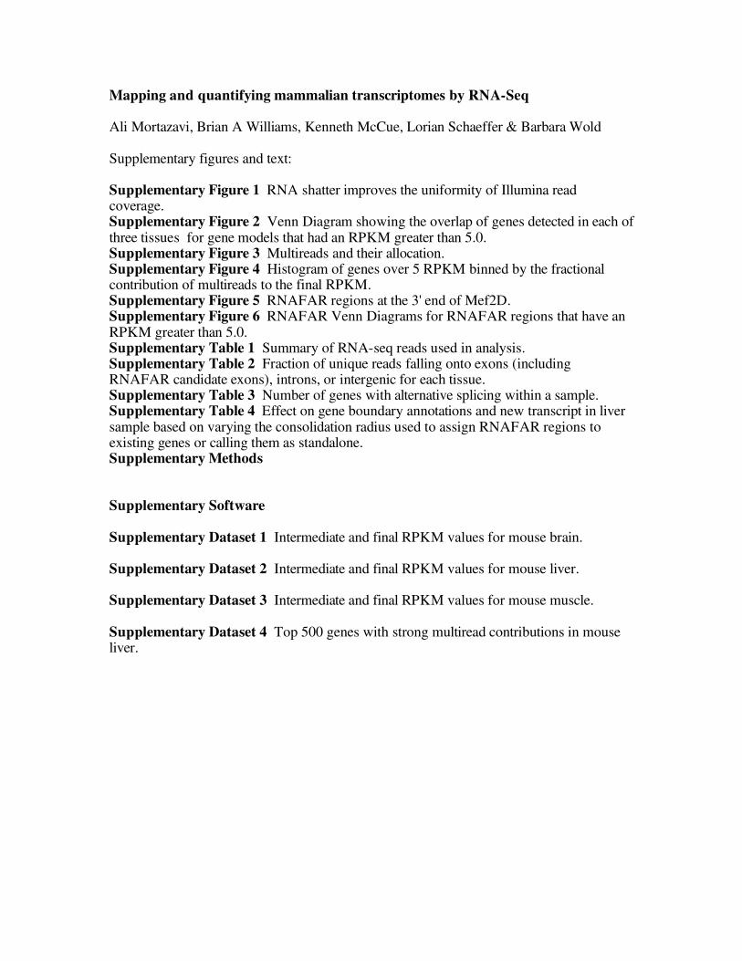
Supplementary Figure 1. RNA shatter improves the uniformity of Illumina read coverage.

A. Uniformity of Illumina sequence read distribution for randomly primed cDNA substrate by fragmenting the RNA template (RNA shatter). Intact RNA samples were primed for reverse transcription using either the RNA shatter protocol, the manufacturer’s protocol (Invitrogen cDNA synthesis kit), or a custom priming protocol designed for use on tiling arrays 11. Uniformity of the distribution of reads was evaluated on a subset of exons in the mouse genome which exceeded a minimal read density threshold in all priming protocols. The Kolmogorov/Smirnoff (KS) statistic was computed for a comparison of the read distribution on each selected exon with a theoretical uniform distribution of reads placed on that exon. The ECDF (empirical cumulative distribution function) of the KS statistics from the exon collection (Y-axis) is plotted against the KS values on the X-axis. Lower KS values indicate a closer approximation to uniformity; thus, the further to the "left" an ECDF is, the more closely that priming protocol fits the model of a uniform distribution of reads across the exons. It is useful to compare the protocols with each other and also with a theoretical best uniformity outcome, which was determined by simulating KS-statistics on the selected exons under the assumption of uniformity of the reads. B. The read distribution for the 2kb desmin transcript in C2C12 muscle cells is shown for the RNA shatter protocol (green) and for the standard randomly primed cDNA protocol (red). The GC content of desmin is mapped in the lower panel, indicating no simple correlation of GC content with peaks of maximal nonuniformity. C. Sequence read coverage of the in vitro synthesized EPR spike-in standard from two different measurements (muscle = red. liver = black) using the RNA shatter


protocol. Coefficient of variation is shown in green. Residual non-uniformity is observed and is quite stereotypic from one sample to another (see text).


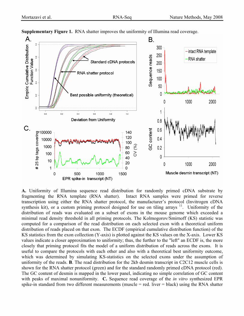
Supplementary Figure 2. Venn Diagram showing the overlap of genes detected in each of three tissues

for gene models that had an RPKM greater than 5.0.


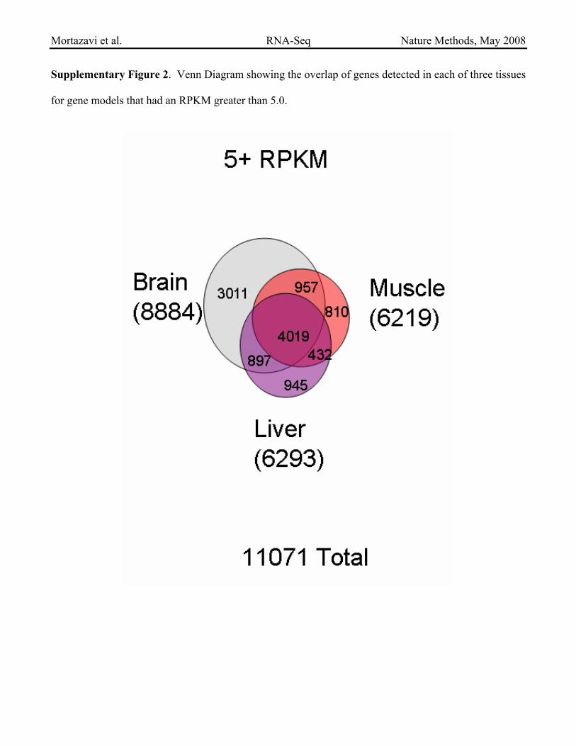
Supplementary Figure 3. Multireads and their allocation.

A. 25bp multireads and their allocation in the mouse genome and muscle transcriptiome. B. 10 kb region

of the ubiquitin Ubb locus is shown. E-RANGE allocates multireads (2-10 occurrences in the genome)

using a weighting function based on the density of uniquely-mapping reads at each paralog (shown in

red)


Supplementary Figure 4. Histogram of genes over 5 RPKM binned by the fractional contribution of

multireads to the final RPKM.


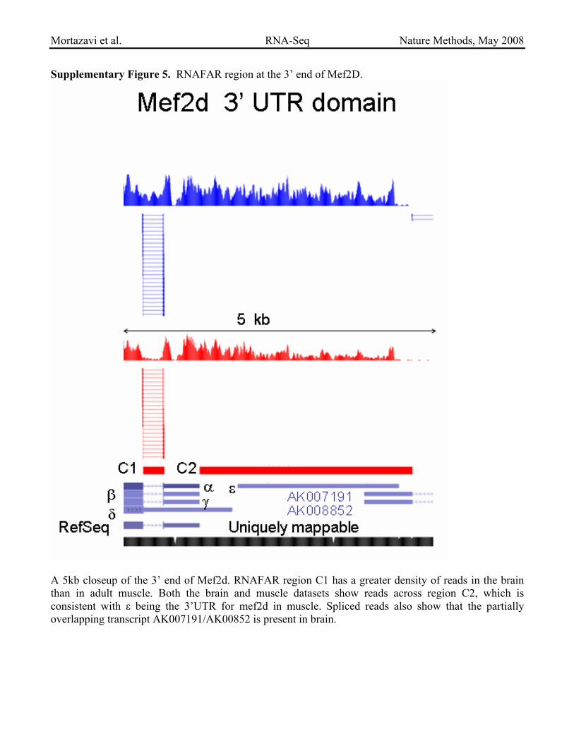
Supplementary Figure 5. RNAFAR region at the 3’ end of Mef2D.

A 5kb closeup of the 3’ end of Mef2d. RNAFAR region C1 has a greater density of reads in the brain than in adult muscle. Both the brain and muscle datasets show reads across region C2, which is consistent with ε being the 3’UTR for mef2d in muscle. Spliced reads also show that the partially overlapping transcript AK007191/AK00852 is present in brain.


Supplementary Figure 6. RNAFAR Venn Diagrams for RNAFAR regions that have an RPKM greater

than 5.0.

596 RNAFAR consolidated regions that are further than 20 kb away from a gene model boundary were

called, with 368 higher than 5 RPKM in one or more tissues.


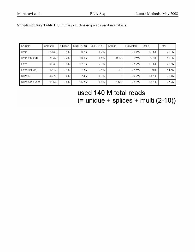
Supplementary Table 1. Summary of RNA-seq reads used in analysis.


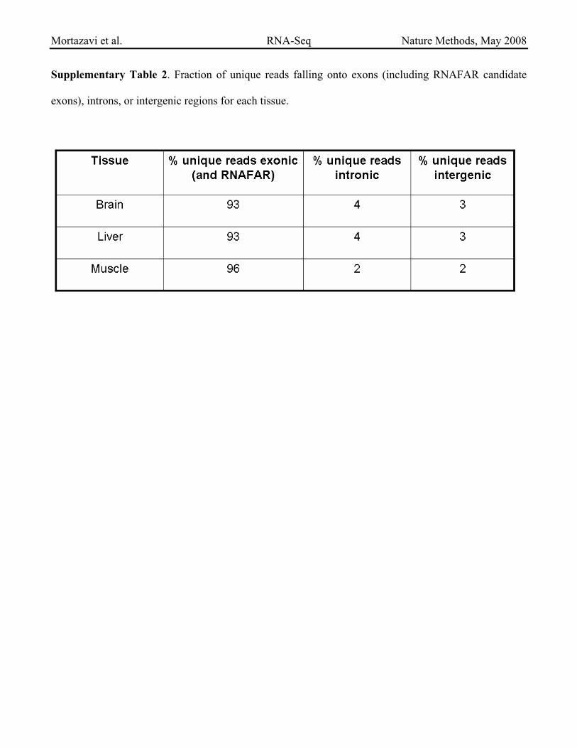
Supplementary Table 2. Fraction of unique reads falling onto exons (including RNAFAR candidate

exons), introns, or intergenic regions for each tissue.


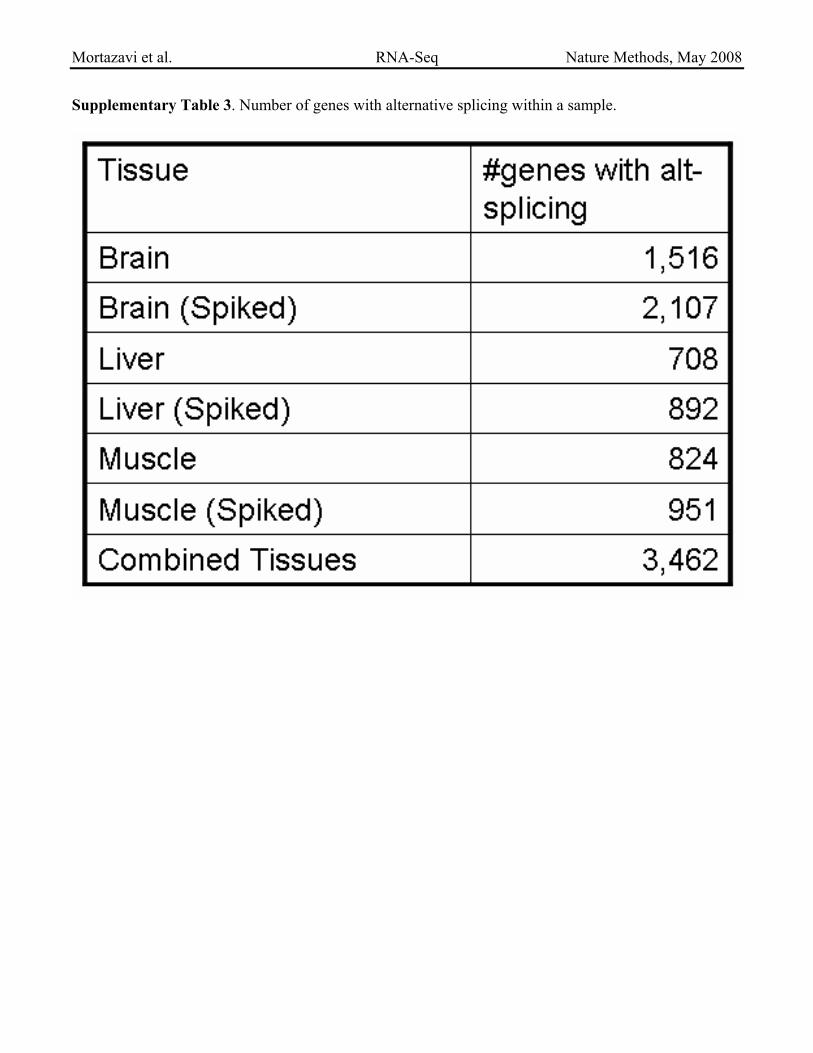
Supplementary Table 3. Number of genes with alternative splicing within a sample.


Supplementary Table 4. Effect on gene boundary annotations and new transcripts in liver sample based

on varying the consolidation radius used to assign RNAFAR regions to existing genes or calling them as

standalone.


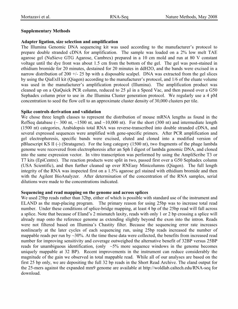
Supplementary Methods Adapter ligation, size selection and amplification The Illumina Genomic DNA sequencing kit was used according to the manufacturer’s protocol to prepare double stranded cDNA for amplification. The sample was loaded on a 2% low melt TAE agarose gel (NuSieve GTG Agarose, Cambrex) prepared in a 10 cm mold and run at 80 V constant voltage until the dye front was about 1.5 cm from the bottom of the gel. The gel was post-stained in ethidium bromide for 20 minutes, destained for 20 minutes in ddH2O, and the bands were excised in a narrow distribution of 200 +/- 25 bp with a disposable scalpel. DNA was extracted from the gel slices by using the QiaExII kit (Qiagen) according to the manufacturer’s protocol, and 1/6 of the eluate volume was used in the manufacturer’s amplification protocol (Illumina). The amplification product was cleaned up on a QiaQuick PCR column, reduced to 25 µl in a Speed Vac, and then passed over a G50 Sephadex column prior to use in .the Illumina Cluster generation protocol. We regularly use a 4 pM concentration to seed the flow cell to an approximate cluster density of 30,000 clusters per tile. Spike controls derivation and validation We chose three length classes to represent the distribution of mouse mRNA lengths as found in the RefSeq database (~ 300 nt, ~1500 nt, and ~10,000 nt). For the short (300 nt) and intermediate length (1500 nt) categories, Arabidopsis total RNA was reverse-transcribed into double stranded cDNA, and several expressed sequences were amplified with gene-specific primers. After PCR amplification and gel electrophoresis, specific bands were excised, eluted and cloned into a modified version of pBluescript KS II (-) (Stratagene). For the long category (1500 nt), two fragments of the phage lambda genome were recovered from electrophoresis after an Sph I digest of lambda genomic DNA, and cloned into the same expression vector. In vitro transcription was performed by using the AmpliScribe T3 or T7 kits (EpiCentre). The reaction products were split in two, passed first over a G50 Sephadex column (USA Scientific), and then further cleaned up over RNEasy Minicolumns (Qiagen). The full length integrity of the RNA was inspected first on a 1.5% agarose gel stained with ethidium bromide and then with the Agilent BioAnalyzer. After determination of the concentration of the RNA samples, serial dilutions were made to the concentrations indicated. Sequencing and read mapping on the genome and across splices We used 25bp reads rather than 32bp, either of which is possible with standard use of the instrument and ELAND as the map-placing program. The primary reason for using 25bp was to increase total read number. Under these conditions of splice-bridge mapping, at least 4 bp of the 25bp read will fall across a splice. Note that because of Eland’s 2 mismatch laxity, reads with only 1 or 2 bp crossing a splice will already map onto the reference genome as extending slightly beyond the exon into the intron. Reads were not filtered based on Illumina’s Chastity filter. Because the sequencing error rate increases nonlinearly at the later cycles of each sequencing run, using 25bp reads increased the number of mappable reads per run by ~30%. At the time these data were collected, the benefits from increased read number for improving sensitivity and coverage outweighed the alternative benefit of 32BP versus 25BP reads for unambiguous identification, (only ~5% more sequence windows in the genome becomes uniquely mappable at 32 BP). Recent improvements in the instrument can reduce considerably the magnitude of the gain we observed in total mappable read. While all of our analyses are based on the first 25 bp only, we are depositing the full 32 bp reads in the Short Read Archive. The eland output for the 25-mers against the expanded mm9 genome are available at http://woldlab.caltech.edu/RNA-seq for download.


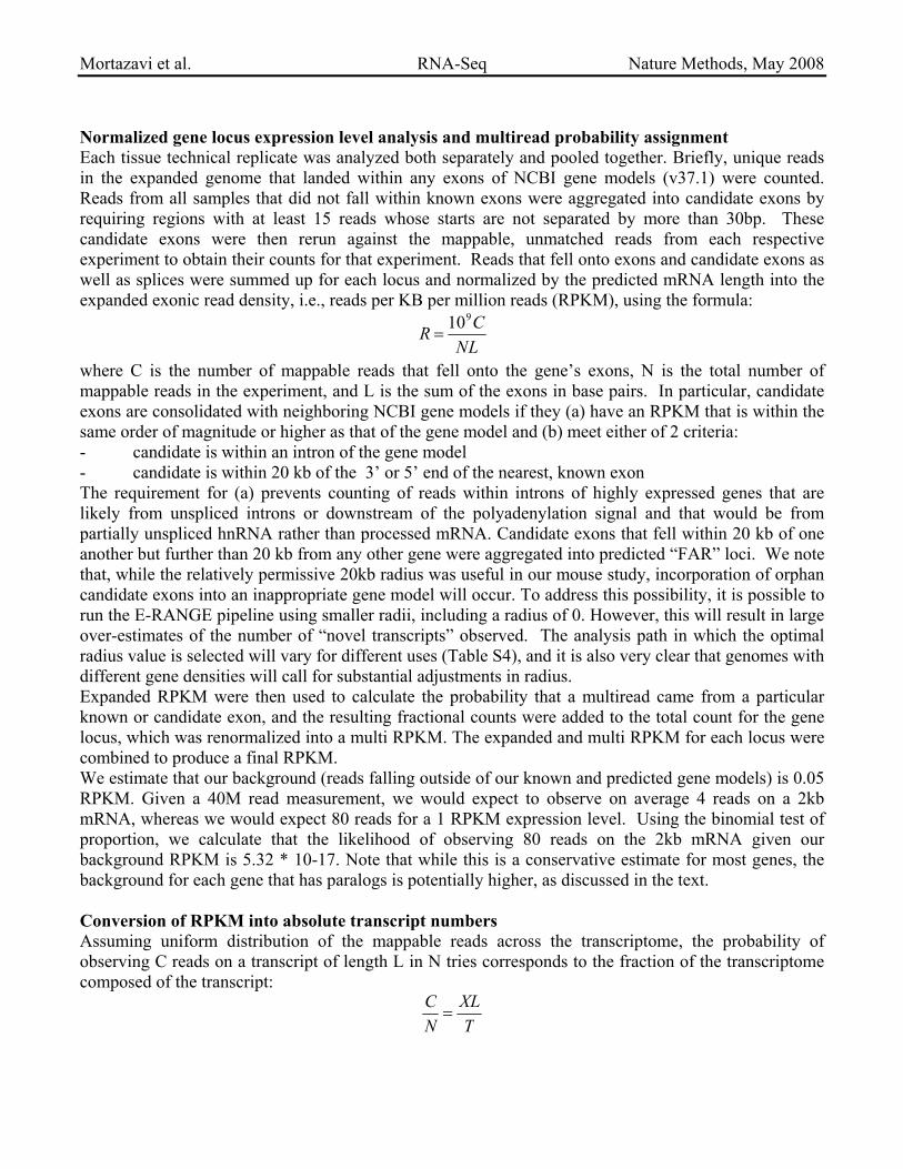
Normalized gene locus expression level analysis and multiread probability assignment Each tissue technical replicate was analyzed both separately and pooled together. Briefly, unique reads in the expanded genome that landed within any exons of NCBI gene models (v37.1) were counted. Reads from all samples that did not fall within known exons were aggregated into candidate exons by requiring regions with at least 15 reads whose starts are not separated by more than 30bp. These candidate exons were then rerun against the mappable, unmatched reads from each respective experiment to obtain their counts for that experiment. Reads that fell onto exons and candidate exons as well as splices were summed up for each locus and normalized by the predicted mRNA length into the expanded exonic read density, i.e., reads per KB per million reads (RPKM), using the formula:

R =109CNL

where C is the number of mappable reads that fell onto the gene’s exons, N is the total number of mappable reads in the experiment, and L is the sum of the exons in base pairs. In particular, candidate exons are consolidated with neighboring NCBI gene models if they (a) have an RPKM that is within the same order of magnitude or higher as that of the gene model and (b) meet either of 2 criteria: - candidate is within an intron of the gene model - candidate is within 20 kb of the 3’ or 5’ end of the nearest, known exon The requirement for (a) prevents counting of reads within introns of highly expressed genes that are likely from unspliced introns or downstream of the polyadenylation signal and that would be from partially unspliced hnRNA rather than processed mRNA. Candidate exons that fell within 20 kb of one another but further than 20 kb from any other gene were aggregated into predicted “FAR” loci. We note that, while the relatively permissive 20kb radius was useful in our mouse study, incorporation of orphan candidate exons into an inappropriate gene model will occur. To address this possibility, it is possible to run the E-RANGE pipeline using smaller radii, including a radius of 0. However, this will result in large over-estimates of the number of “novel transcripts” observed. The analysis path in which the optimal radius value is selected will vary for different uses (Table S4), and it is also very clear that genomes with different gene densities will call for substantial adjustments in radius. Expanded RPKM were then used to calculate the probability that a multiread came from a particular known or candidate exon, and the resulting fractional counts were added to the total count for the gene locus, which was renormalized into a multi RPKM. The expanded and multi RPKM for each locus were combined to produce a final RPKM. We estimate that our background (reads falling outside of our known and predicted gene models) is 0.05 RPKM. Given a 40M read measurement, we would expect to observe on average 4 reads on a 2kb mRNA, whereas we would expect 80 reads for a 1 RPKM expression level. Using the binomial test of proportion, we calculate that the likelihood of observing 80 reads on the 2kb mRNA given our background RPKM is 5.32 * 10-17. Note that while this is a conservative estimate for most genes, the background for each gene that has paralogs is potentially higher, as discussed in the text. Conversion of RPKM into absolute transcript numbers Assuming uniform distribution of the mappable reads across the transcriptome, the probability of observing C reads on a transcript of length L in N tries corresponds to the fraction of the transcriptome composed of the transcript:

CN=

XLT


where X is the copy number of the transcript and T is the length of the transcriptome in base pairs. We can substitute final RPKMs to get:

X =C

NLT =

R109 T

We can either derive T from the starting amount of mRNA (assuming 100% efficiency in cDNA synthesis), or by estimating T from spike-in data.

mapping and quantifying mammalian transcriptomes by … · mapping and quantifying mammalian...

Documents