Mapping Aquifer Systems with AirborneElectromagnetics in the Central Valley ofCaliforniaby Rosemary Knight1, Ryan Smith2, Ted Asch3, Jared Abraham3, Jim Cannia3, Andrea Viezzoli4, and Graham Fogg5

AbstractThe passage of the Sustainable Groundwater Management Act in California has highlighted a need for cost-effective ways to

acquire the data used in building conceptual models of the aquifer systems in the Central Valley of California. One approach would bethe regional implementation of the airborne electromagnetic (AEM) method. We acquired 104 line-kilometers of data in the TulareIrrigation District, in the Central Valley, to determine the depth of investigation (DOI) of the AEM method, given the abundance ofelectrically conductive clays, and to assess the usefulness of the method for mapping the hydrostratigraphy. The data were highquality providing, through inversion of the data, models displaying the variation in electrical resistivity to a depth of approximately500 m. In order to transform the resistivity models to interpreted sections displaying lithology, we established the relationshipbetween resistivity and lithology using collocated lithology logs (from drillers’ logs) and AEM data. We modeled the AEM responseand employed a bootstrapping approach to solve for the range of values in the resistivity model corresponding to sand and gravel,mixed coarse and fine, and clay in the unsaturated and saturated regions. The comparison between the resulting interpretationand an existing cross section demonstrates that AEM can be an effective method for mapping the large-scale hydrostratigraphy ofaquifer systems in the Central Valley. The methods employed and developed in this study have widespread application in the use ofthe AEM method for groundwater management in similar geologic settings.

IntroductionTo ensure a secure food supply, many agricultural

regions of the world require reliable sources of surfacewater and/or groundwater to meet irrigation needs. TheCentral Valley of California is one such region. Covering50,000 km2, bounded by the Sierra Nevada to the east andthe Coast Ranges to the west, the valley yields a third of

1Corresponding author: Department of Geophysics, StanfordUniversity, 397 Panama Mall, Stanford, CA 94305-2210; (650)736-1487; fax: (650) 725-7344; rknight@stanford.edu

2Department of Geophysics, Stanford University, 397 PanamaMall, Stanford, CA 94305-2210.

3Aqua Geo Frameworks, 130360 County Road D, Mitchell, NE,69357.

4Aarhus Geophysics Aps, Lollandsgade 52, Aarhus C, 8000,Denmark.

5Department of Land, Air and Water Resources, University ofCalifornia, Davis, One Shields Avenue, Davis, CA 95616.

Article impact statement: Airborne electromagnetic dataprovide the critical information needed to develop conceptualmodels of the aquifer systems in the Central Valley of California.

Received August 2017, accepted March 2018.© 2018 The Authors. Groundwater published by Wiley Periodi-

cals, Inc. on behalf of National Ground Water Association.This is an open access article under the terms of the Creative

Commons Attribution License, which permits use, distribution andreproduction in any medium, provided the original work is properlycited.

doi: 10.1111/gwat.12656

the produce grown in the United States valued at $17billion dollars per year (U.S. Geological Survey 2016).Much of the irrigation water in the valley has historicallybeen taken from surface water—the rivers, lakes, andreservoirs replenished by winter storms and the springmelting of the snow pack in the Sierra Nevada. This wateris provided through a series of federal, state and privateirrigation canals, dams and lakes. In times of drought,most recently in the periods 2007 to 2009 and 2012 to2016, when surface water deliveries were substantiallyreduced, the only way to meet irrigation needs has beenthrough extensive pumping of groundwater. This hasexacerbated an already serious problem in the CentralValley, where some areas have experienced decliningwater levels for several decades. Drought conditions haveled to further lowering of groundwater levels, due toincreased pumping and decreased recharge, causing wellsto go dry and, in some areas, significant subsidence of theground surface. The overdraft has been so significant, thatthere are now approximately140 million acre-feet (MAF)of unused groundwater storage space in the Central Valley,a value calculated based on the estimated differencebetween predevelopment and current conditions (TheNature Conservancy 2016). In contrast, the total surfacewater storage capacity in California is 42 MAF.

The alluvial sedimentary geology of the CentralValley is typically composed of more than 50% to

NGWA.org Vol. 56, No. 6–Groundwater–November-December 2018 (pages 893–908) 893

70% fine-grained deposits dominated by silt and claybeds. These silts and clays make the groundwater basinconfined to semi-confined, significantly impeding verticalgroundwater flow. Within this geologic system arenetworks of sand and gravel that both constitute theaquifer system and provide pathways for recharge. Thesustainable management of the groundwater resources ofthe Central Valley, now required with the passage of theSustainable Groundwater Management Act (SGMA) bythe California Legislature in 2014, highlights the need tobetter understand the hydrostratigraphy of the subsurfaceto improve the conceptual models of the aquifer systemsand provide the information needed to inform manage-ment decisions. Mapping the locations of the sand andgravel networks would make it possible to select the bestlocations for surface spreading techniques so that rechargecould be dramatically increased, and repressurization ofthe confined aquifer networks could be accomplished.Mapping of the aquifer systems could also help assessthe vulnerability of an area to subsidence associated withgroundwater withdrawal, as subsidence in the CentralValley occurs primarily in areas where there are numerousclays layers interlayered with the sands and gravels (Fauntand Sneed 2015). In addition, accurate conceptual modelscould guide the siting of expensive monitoring wells.

The key question is then: How do we map the aquifersystems in the Central Valley in a cost-effective way? Wepropose regional implementation of the airborne electro-magnetic (AEM) method to obtain information neededabout the hydrostratigraphy of the aquifer systems. Thereare various AEM methods available, all of which usean airborne platform to move geophysical sensors overan area to map out subsurface variations in electricalresistivity to depths of approximately 500 m (dependingon the electrical resistivity). Vertical resolution is on theorder of meters to tens of meters. Lateral resolution alongthe flight lines is typically 30 m; between the flight lines itis determined by the line spacing, which is set accordingto the objectives of the survey and can range from250 m to 30 km. Given the relationship between electricalresistivity and the properties of the subsurface geologicalmaterials, AEM data can be used, along with existinglithologic information available from drillers’ logs, todevelop a model of the large-scale (tens to hundreds ofmeters) hydrostratigraphic packages that define the archi-tecture of the aquifer systems. The AEM method has beenused throughout the world for groundwater explorationand aquifer mapping (e.g., Sattel and Kgotlhang 2004;Podgorski et al. 2013). The various methods that havebeen used to develop the hydrostratigraphic model aredescribed in a recent paper by Christensen et al. (2017)and include both knowledge-driven cognitive approaches(e.g., Jørgensen et al. 2013) and geostatistical approaches(e.g., Marker et al. 2015).

We conducted a pilot study to assess the use ofAEM to map the aquifer systems in the Central Valley ofCalifornia. There had been one private survey completed,so this represented an opportunity to acquire the firstpublicly available dataset in the valley. We elected to

use the SkyTEM system. An important factor in thisselection was the ability of the system to provide theresolution required within the study area; studies haveshown that the SkyTEM system can provide good res-olution in similar environments (Bedrosian et al. 2015).The SkyTEM system, originally developed by AarhusUniversity (Sørensen and Auken 2004), was specificallydesigned with a dual moment transmitter that allows fornear-surface as well as deep penetration. SkyTEM hasbeen used over the past 15 years in Denmark to acquire60,000 line kilometers of data covering 15,000 km2.Together with the airborne sensor, processing softwarewas developed and a national data repository establishedthat enables access to processed data for water authorities,water suppliers, municipalities, and others (Thomsenet al. 2004; Auken et al. 2009; Møller et al. 2009).

The demand for acquiring these AEM data inDenmark has been driven by groundwater legislation thatrequires that all municipalities characterize and managethe groundwater systems. AEM has been found to be themost cost-effective way to get the subsurface coverageneeded for compliance with this regulatory requirement;a significant benefit being that there is no need for landaccess. In California, SGMA requires that local authoritiesassess the state of their groundwater basins and developplans for the sustainable management of groundwater. Theacquisition of AEM data throughout California could playa central role in providing critical information that caninform the development of groundwater models, guiderecharge efforts, assess geologic controls on observedsubsidence, and aid in siting of monitoring wells.

The location selected for our study, shown inFigure 1, is in the Tulare Irrigation District in the SanJoaquin Valley that, with the Sacramento Valley tothe north, makes up the Central Valley. There havebeen extensive, chronic groundwater level declines andassociated problems such as subsidence in this areabetween 2007 and 2009 (Farr and Liu 2014; Smith et al.2017). The geology in this area is typical of that foundthroughout the Central Valley, so AEM performance atthis location should be representative of how it wouldperform elsewhere in the valley. The first question weposed was related to the quality of the acquired data: howeffective would the AEM method be in imaging beneaththe shallow, electrically conductive clays commonlyfound in the Central Valley? The second question weposed was related to the interpretation of the resistivitymodels obtained through inversion of the acquired AEMdata. In Denmark, the 15 years of working with AEMdata have involved extensive analysis of resistivity datafrom geophysical measurements (AEM, ground-basedand borehole) and lithologic information from wells tobuild a national atlas that can be used derive lithologyinformation from resistivity measurements (Møller et al.2009; Christiansen et al. 2014; Barfod et al. 2016).Nothing of this sort currently exists in California. Thequestion we posed: Could we work with the resistivitymodels and the limited well data to obtain informationabout the architecture of the aquifer systems, mapping

894 R. Knight et al. Groundwater 56, no. 6: 893–908 NGWA.org

Figure 1. Location map showing the study area, the TulareIrrigation District, outlined in brown. Data sources: U.S.National Parks Service, U.S. Census Bureau, CaliforniaDepartment of Water Resources (2003).

out key hydrostratigraphic packages? Answering thesetwo questions, related to the ability to acquire and theninterpret high quality data, was an essential first step indetermining whether the AEM method could be reliablyused for mapping the aquifer systems in the CentralValley. If so, this would be a new way of obtainingcritical information needed for the implementation ofSGMA, and could significantly transform the approach togroundwater management in California. While the focusof this study was the Central Valley of California, thefindings and the new methodologies developed will havemuch broader impacts, advancing the use of AEM forimaging alluvial aquifer systems throughout the world.

Description of Study AreaFigure 2 is an image showing subsidence measured

between 2007 and 2010 in the area of the Tulare IrrigationDistrict; we derived this image from InterferometricSynthetic Aperture Radar (InSAR) data. InSAR is amethod that can provide the change in ground elevationover time with accuracy on the order of millimetersto centimeters (Madsen and Zebker 1998; Rosen et al.2000). The change in phase measured between twosatellite passes is used to form an interferogram fromwhich the change in elevation is calculated. To obtainthe subsidence map in Figure 2, we used data from the

Figure 2. Image showing InSAR-mapped subsidencebetween 2007 and 2010 in the area of the Tulare IrrigationDistrict (outlined in yellow), along with the AEM flight lines(black) and the locations of the lithology logs (red dots).Also shown as a blue line is the location (A-A′) of the usedportion of the cross section provided by the Kaweah DeltaWater Conservation District.

Advanced Land Observing Satellite (ALOS), which has anL-band radar system with a wavelength of approximately24 cm. This relatively long wavelength is more effective inagricultural areas, because it is not as easily decorrelatedby vegetation. We processed 82 interferograms over thetime frame 2007 to 2010 and used the small baselinesubset method (Berardino et al. 2002) to calculate therelative motion over time. We then used this time seriesto solve for the mean velocity during the study period. Ascan be seen in Figure 2, subsidence reached a maximumvalue of 26 cm/year between 2007 and 2010.

Our flight lines, shown in Figure 2, covered 104line-kilometers and were selected to go from the centerof the subsidence bowl to an area with little, to no, subsi-dence. Survey flight planning included adherence to U.S.Federal Aviation Administration (U.S. FAA) regulationsregarding flying and towing cargo over infrastructure,including not flying over buildings and large highwaysand flying well above power lines. The lines werespaced approximately 1 km apart in order to conduct asmall-scale reconnaissance of the area of interest.

There are numerous wells in the study area, manywith drillers’ logs that describe lithology; these wereobtained from the California Department of WaterResources. The majority of the wells (∼80%) are less than100 m deep, but we were able to use lithology (drillers’)logs from 12 wells (shown in Figure 2) within approxi-mately 500 m of the flight lines that reach at least 150 m.The lithology logs describe a shallow sand and gravelaquifer, overlying a clay layer, 0 to 20 m thick, referred toas the Corcoran Clay. Beneath the Corcoran Clay, the lim-ited well data suggest another sand and gravel aquifer unitwith interlayered clays. There is one resistivity log within1 km of a flight line, from well 20S23E14, which showsthe location of the Corcoran Clay, as well as the alternat-ing sand to clay nature of the upper and lower aquifer.

In addition to the lithologic logs, we had a reportwith cross sections, provided by the Kaweah Delta Water

NGWA.org R. Knight et al. Groundwater 56, no. 6: 893–908 895

Conservation District (Fugro West 2007), which describedupper and lower aquifer units that are separated by theCorcoran Clay. The upper aquifer is described as Quater-nary older alluvium (oxidized) and the lower aquifer isdescribed as Quaternary older alluvium (reduced). Bothaquifers are interpreted to have numerous interbedded siltsand clays, with the lower aquifer interpreted to have morefine-grained material than the upper aquifer (Fugro West2007). The Corcoran Clay, described in the report as Qua-ternary lacustrine and marsh deposits, pinches out in theeastern part of the section. At the base of the lower aquiferis an impermeable unit described as Pliocene and Pleis-tocene (questionable) continental deposits.

Acquiring the AEM Resistivity Model:Methodology and Results

The AEM method has been used for many years tomap geology (Palacky 1981) and, in the last 10 or so years,has been widely used to map groundwater prospects.The theory behind the method is described in Ward andHohmann (1988). In the SkyTEM system used in thisstudy, all of the hardware required for data acquisitionis suspended beneath a helicopter, which moves overthe land surface at approximately 80 to 100 km/h withthe frame hanging approximately 30 m above the groundsurface. Current flowing in a transmitter loop generatesa primary magnetic field. The termination of currentcauses a time-varying decay in the produced magneticfield which causes eddy currents to flow at various depthsbeneath the land surface. The less electrically resistivethe region, the stronger the current and the more slowlythe current decays. The eddy currents generate their ownsecondary magnetic fields which are measured at thereceiver mounted on the transmitter loop. The strengthof the field and the time dependence contains informationabout how current flows through the ground. The acquireddata are inverted to obtain a model of the spatial variationin electrical resistivity of the subsurface material.

Airborne data were acquired using the SkyTEM508 system on October 27, 2015. Although data wereacquired approximately every 2.5 m along each of theflight lines, the dual moment mode, in which the datawere acquired and averaged, resulted in an effective EMsounding spacing of 30 m along each line.

The acquired data were inverted using the AarhusWorkbench (HydroGeophysics Group 2011). The pro-cedure applied to the data processing, including noiseassessment, follows that detailed in Auken et al. (2009).We then performed laterally constrained inversions(Auken et al. 2009) where correlation along the flightline is imposed on the inversion. This was followedby spatially constrained inversions, defined in Viezzoliet al. (2008) as a methodology to impose correlationacross survey lines. The values of the parameters used toenforce spatial coherency, from equation 12 in Viezzoliet al., were A = 1.5, B = 30 m, b = 0.75. These weredetermined based on both prior geological knowledgeand empirically, that is, testing a few variations while

analyzing data misfit. For the starting model we useda resistivity everywhere of 30 � m. While no lithologylogs or electrical logs were used as constraints in theinversion (the electrical log was too far, >150 m, from theflight lines), they were used postinversion for qualitativeanalysis and comparison with the AEM inversion results.

Figure 3 presents the resulting resistivity model forLine 3 (the position of which is shown in Figure 2). The Yposition in this figure is the distance along the survey line.Gaps in the image are due to electromagnetic couplingof the AEM acquisition system with ground interferencesuch as power lines and cathodically protected pipelines.The affected soundings were filtered and then manuallyedited out of the data set prior to inversion. Each pixel inthe resulting resistivity model has an assigned resistivityvalue. The size of a pixel corresponds to the spatial reso-lution, both horizontal and vertical, at that location. Hori-zontal resolution along the flight line is based on the AEMsounding separation (about 3 m) and the number of sound-ings averaged during processing (10 soundings on aver-age). In this study the processed sounding separation was30 m. Large gaps due to decoupling of electromagneticnoise will locally negatively impact the horizontal resolu-tion. The ability to resolve features decreases with depthper the fundamental physics of the technique. As depthincreases, typically each pixel in the resistivity model, forthis acquisition system, increases in thickness by approxi-mately 1.1 times the thickness of the previous layer. In theresistivity model shown in Figure 3, the pixels at the topof the section have a vertical dimension of 3 m, increasingto approximately 14 m at 100 m depth, and approximately48 m at 400 m depth. This approach, of inverting for elec-trical resistivity in a multilayer model with layers of fixedthicknesses, is commonly referred to as smooth model. Weelected to use this type of model because the many layersare needed to accommodate the complexity of the geologicsetting (e.g., the discontinuous clay layers). In addition,this approach allows us to explore, relatively easily, pos-sible subtle variations in the electrical resistivity structure.

The depth of investigation (DOI), as applied here,plays a critical role in data interpretation. The DOI is anumerical estimation of the depth below which the reso-lution of a model, obtained from the numerical inversion,diminishes. This loss of model resolution is primarily dueto the limitations of the method including: the equipmentand methodology used for data acquisition, the noise inthe data, and the resistivity structure (the geology) beinginvestigated (Christiansen and Auken 2012). The AarhusWorkbench uses inverted model sensitivities (componentsof the inversion Jacobian matrix) determined during thelast inversion step, along with an estimate of data uncer-tainty, to calculate the DOI’s (Christiansen and Auken2012). The Jacobian matrix is the sensitivity of the datato perturbations at the current location in model-space.As such, the Jacobian is also a representation of thesensitivity of changes in the model to the observed data.The last step in this process is calculation of the cumula-tive sensitivities, produced by summing up the individualthickness-normalized sensitivities, starting with the

896 R. Knight et al. Groundwater 56, no. 6: 893–908 NGWA.org

Figure 3. Resistivity model derived from inversion of AEM data from Line 3. The Y position is the distance along the surveyline. The estimated water table is shown as a dashed line, while the upper depth of investigation is shown as a dotted line.The model ends at the estimated lower depth of investigation.

bottom layer. Two cumulative-sensitivity thresholds areselected to represent what are known as the “upper” and“lower” depths of investigation. We selected cumulative-sensitivity thresholds of 0.6 and 0.1 for calculation of theupper and lower DOI’s. In Figure 3 the upper estimateof the DOI is represented as a dotted line and the lowerestimate of the DOI coincides on this particular line withthe base of the displayed profile section.

In Figure 3 notice that the upper DOI ranges inelevation from a maximum of about −300 m down to anelevation of about −375 m. This is not a large range atthese elevations. It is a bit shallower over the resistivezone on the southern end (the left side) of Line 3 anda little deeper on the northern end (right side) of Line3. Typically, the DOI is deeper in resistive material andshallower in conductive materials. The key to interpretingthe upper DOI in Figure 3 is to examine the resistivityvalues in the first 200 m. On the south end of the linethere is more conductive material between elevations 0 to−100 m. On the northern end of the line, there is moreresistive material between elevations of +75 m and −50to −100 m. These differences in the first 200 m of thesubsurface are influencing the character of the upper DOI.The lower DOI, at the bottom of the section along thisline, displays an irregular character along the northern endof Line 3, indicating that the model’s sensitivity to theresistivity values at depth in those locations is quite low.

For the depth of the water table (shown in Figure 3)we used the interpolation of water level data, measuredbetween September 1, 2015 and November 25, 2015, pro-vided by the California Department of Water Resources,2016, Groundwater Information Center Interactive MapApplication: https://gis.water.ca.gov/app/gicima/. Thedepth of the water table was estimated to vary in the studyarea between about 47 and 60 m. Given that the distancebetween wells used for the interpolation was on the orderof kilometers, variations in the water table at the subkilo-meter scale will not be captured in these data. Most of the

highest resistivity values in the profile section presented inFigure 3 are found in the region above the estimated watertable. This can be seen in a comparison of the histogramof all the AEM inversion resistivity values from the regionabove the water table (Figure 4a) with the histogram ofvalues in the region below the water table (Figure 4b).Below the water table, resistivity values range from 6 to43 � m. Above the water table, resistivity values rangefrom 8 to 150 � m; we display in the figure the counts outto 60 � m as only 2% of the data had resistivity valuesgreater than 50 � m. The difference in resistivity valuesabove and below the water table becomes important inthe interpretation of the resistivity model.

The Resistivity-Lithology Relationship:Methodology and Results

The relationship between resistivity and lithology is atthe core of the use of any geophysical electromagnetic orresistivity method to map out the variation in subsurfacelithology. The extensive literature studying the resistivity-lithology relationship is reviewed by Knight and Endres(2005) and briefly summarized here, highlighting what weexpect to be the dominant factors linking resistivity andlithology in our study area.

In sediments and sedimentary rocks with water in thepore space, the primary mechanism for electrical conduc-tion is typically ionic conduction through the pore water.As a result, the electrical resistivity tends to decreaseas the volume of water-filled porosity (equivalent tovolumetric water content) increases and will also decreaseas the salinity of the water increases. In the main aquifersof the Tulare Irrigation District, there are no reports ofsignificant variation in salinity of the pore water so, inthis study, we assumed that pore water chemistry doesnot affect electrical resistivity. Further work is needed toincorporate water quality into the interpretation. For our

NGWA.org R. Knight et al. Groundwater 56, no. 6: 893–908 897

0 20 40 60resistivity, ohm-m

0

500

1000

1500

2000

0 20 40 60resistivity, ohm-m

0

2000

4000

6000

coun

tco

unt

(a)

(b)

Figure 4. Histograms of estimated resistivity values for theregion (a) above the water table and (b) below the watertable.

study area, if we consider only electrical conduction dueto ionic conduction through the pore water, we wouldexpect to see, as observed, higher resistivity values abovethe water table where the sediments are unsaturated.We would also expect to see resistivity decrease as theporosity of the material increases.

A second mechanism that contributes to electricalconduction in sediments is surface conduction, whichoccurs due to the presence of a high concentration ofions associated with the electrical double layer at thesolid/water interface. While surface conduction can occurin any material, it is most significant when clays arepresent due to their high surface area. The presence ofsurface conduction causes electrical resistivity to decreaseas the surface-area-to-volume ratio increases; that is,resistivity will decrease as the grain size decreases and asclay content increases. For the purposes of our study, ifsurface conduction contributes to the measured electricalresistivity, we would expect to observe the highestresistivity values in the gravels and sands, with resistivitydecreasing in silts, and further decreasing in the clays.

Given the absence of any database comparing resis-tivity and lithology data in California, we began our anal-ysis of the resistivity-lithology relationship with a reviewof all available geological data and then a comparison withthe resistivity values in the AEM resistivity model. Thisestablished method, referred to as Method 1, involves thesteps outlined in Jørgensen et al. (2003) and Høyer et al.(2015), and involves the development of a conceptualgeological model followed by comparing lithological andborehole geophysical logs to the AEM resistivity model. A

Table 1Resistivity Ranges Correlated with the VariousLithologic Units Based on Interpretation of the

Geologic Units, Referred to as Method 1

Inverted Resistivity Values (� m) Interpreted Lithology

6 10 Clay10 13 Silty clay13 16 Clayey silt16 19 Interbedded

sand/clay/silt19 150 Sands/gravels

critical step is to identify key lithological units in the studyarea that could be used for resistivity-lithology correla-tions. This was assisted by examination of cross sectionsB-B′ and C-C′ in the Fugro West report (Fugro West2007). The lithology logs presented in that report, showingvarious units of clays, sands, and gravels, in combinationwith the 12 lithology logs we had available, provided keylithology information as well as location information ofrepresentative lithologies to which the resistivity modelscould be correlated. Based on these resistivity-lithologycorrelations, Table 1 was developed. Note, in defining thelithology categories, we used the terms seen in the FugroWest report and the drillers’ logs.

The ranges in the resistivity values presented inTable 1 encompass the information from the AEM data,published cross sections, and lithology logs but are limitedby the relatively small number of lithology logs close tothe survey flight lines, the shallow depth of some of thelithology logs, and by the difficulty in separating out theresistivities above the water table from below the watertable. We therefore decided to explore a second approach.

Our second approach, referred to as Method 2,involved the development of a new methodology thatused the 12 lithology logs and the AEM resistivity modelto quantitatively solve for the ranges of resistivity valuesthat correspond to defined lithologies in the study area.At the core of this method is a key point: What wewanted was the relationship between the AEM-measuredresistivity and lithology, not between resistivity measuredby some other method (e.g., resistivity logging) andlithology; so we used the AEM resistivity values. Oneof the limitations in our approach, common to anyother approach that could be used in this study area,was the lack of information about lithology belowapproximately 150 m. We assumed that the establishedresistivity-lithology transform was valid at greater depthsbut this is an issue that requires further study.

We conducted a separate analysis for the regionsabove and below the water table; a change in watercontent will result in a large change in the resistivity ofa material so it is important to develop the resistivity-lithology relationship in a way that accounts for this.Based on a review of the lithologic logs, and given thesparsity of independent lithologic information, we defined

898 R. Knight et al. Groundwater 56, no. 6: 893–908 NGWA.org

Lithology Log AEM pixel

t1

t2

tAEMAEMt3

t4

t5

layer 1: sand & gravel

layer 2: mixed

layer 3: sand & gravel

layer 5: sand & gravel

layer 4: clay

ρsg

ρsg

ρmixed

ρsg

ρ

ρclay

Figure 5. Schematic illustrating the approach, Method 2,taken to mathematically relate the lithology log and the AEMdata to determine the ranges of resistivity values (i.e., ρsg,ρmixed, and ρclay) for the three lithologic units, sand andgravel, mixed fine and coarse, and clay. The relationshipuses the resistivity value ρAEM from the pixel in the AEMmodel closest to the lithology log, the thicknesses (t) of thevarious units in the lithology log (here t1, t2, t3, t4, t5) andthe thickness of the AEM pixel tAEM.

three lithologies below the water table: sand and gravel,mixed fine and coarse, clay. There was limited mention ofmixed fine and coarse materials in the shallower section,so we reduced the lithology categories in the region abovethe water table to consider only sand and gravel, and clay.We converted the descriptions in all lithology logs to thesecategories. The intervals that we classified as “mixed fineand coarse” had variable descriptions: silt, sandy clay,silty sand and fine sand. We then systematically workedthrough the 12 lithology logs, from ground level to thedeepest layer described, and identified the pixels in theAEM resistivity model that were closest to the location ofthe layers described in the lithology logs.

A schematic of the basic steps in our approach,Method 2, is shown in Figure 5. On the left we havethe layers described in a lithology log; on the right wehave the closest AEM pixel. What is shown here is notan actual log but given as an example to explain ourmethodology using the three lithologies defined belowthe water table. Starting at the top of the lithology log,each layer has an assigned lithology (sand and gravel,mixed fine and coarse, or clay) and a thickness t i wherei corresponds to the number of the layer. In the logs,the thickness of each described lithologic layer typicallyranges from 1 to 2 m. We assigned to each layer theresistivity corresponding to the lithology: ρsg, ρmixed, andρclay for the resistivity of sand and gravel, mixed fineand coarse, and clay, respectively. It is important to notethat while we have used a single variable to represent theresistivity of each lithology, there will always be a rangeof resistivity values due to spatial variation in the watercontent, composition, and pore structure.

On the right in Figure 5 is a pixel from the AEMresistivity model that is closest to the well for which wehave the lithology log. In this study, we worked with

10 15 20 25 30 35

resistivity, ohm-m

0

50

100

150

200

250

300

coun

t

claymixed fine and coarsesand & gravel

Figure 6. Resistivity values determined for clay, mixed fineand coarse, and sand and gravel in the region below thewater table using Method 2. These values were obtained witha bootstrap analysis using all depth intervals below the watertable in the 12 lithology logs and corresponding resistivityvalues from the AEM resistivity model.

all of the depth intervals in the 12 lithology logs andfound that the closest AEM pixels were located on average250 m away from the wells, with the separation distancesranging from 50 m to 1 km. We made the reasonableassumption that the lithology sampled in the AEMmeasurement was that shown in the lithology log. Asshown in Figure 5, the AEM measurement does not havethe vertical resolution to resolve the resistivity structureat the scale of the individual layers. What is derivedfrom the AEM measurement is a larger-scale resistivityvalue referred to as ρAEM. The vertical dimension ofthe AEM pixel, denoted in the figure as tAEM, is thevertical resolution of the AEM measurement at that depth.This varied from approximately 3 m at the surface toapproximately 10 m at the depth of the deepest layers usedin this analysis. We set up a relationship between ρAEM

and the resistivity values in the corresponding layers.The physics of the AEM measurement results in a formof averaging of the resistivity values in the individuallayers that can be described, to first order, by thefollowing relationship between the layer resistivity valuesand ρAEM:

ρAEM =(

n∑i=1

ti

tAEM

1

ρi

)−1

(1)

where for n layers, i , as defined above, refers to the layerand ρi is the layer resistivity which will be ρsg, ρmixed,or ρclay. This relationship can be derived by representing

NGWA.org R. Knight et al. Groundwater 56, no. 6: 893–908 899

each layer by a resistor with resistance Ri = (ρi L)/(t i W ),where L is the length of each layer in the direction parallelto the orientation of the field lines and t i W is the cross-sectional area of each layer perpendicular to the field lines.The orientation of the electric field lines during the AEMmeasurement is such that the total measured resistance,RAEM = (ρAEML)/(tAEMW ), can be estimated by addingthe “layer resistors” in parallel. This assumes that thefield lines are parallel to the layering; this is a reasonableapproximation.

Assuming constant values of resistivity for ρsg,ρmixed, and ρclay, the above equation can be re-writtenfor every depth interval where we have layers describedin a lithology log and a nearby AEM resistivity value, asfollows:

ρAEM =((

tsg

tAEM

) (1

ρsg

)+

(tmixed

tAEM

) (1

ρmixed

)+

(tclay

tAEM

) (1

ρclay

))−1

. (2)

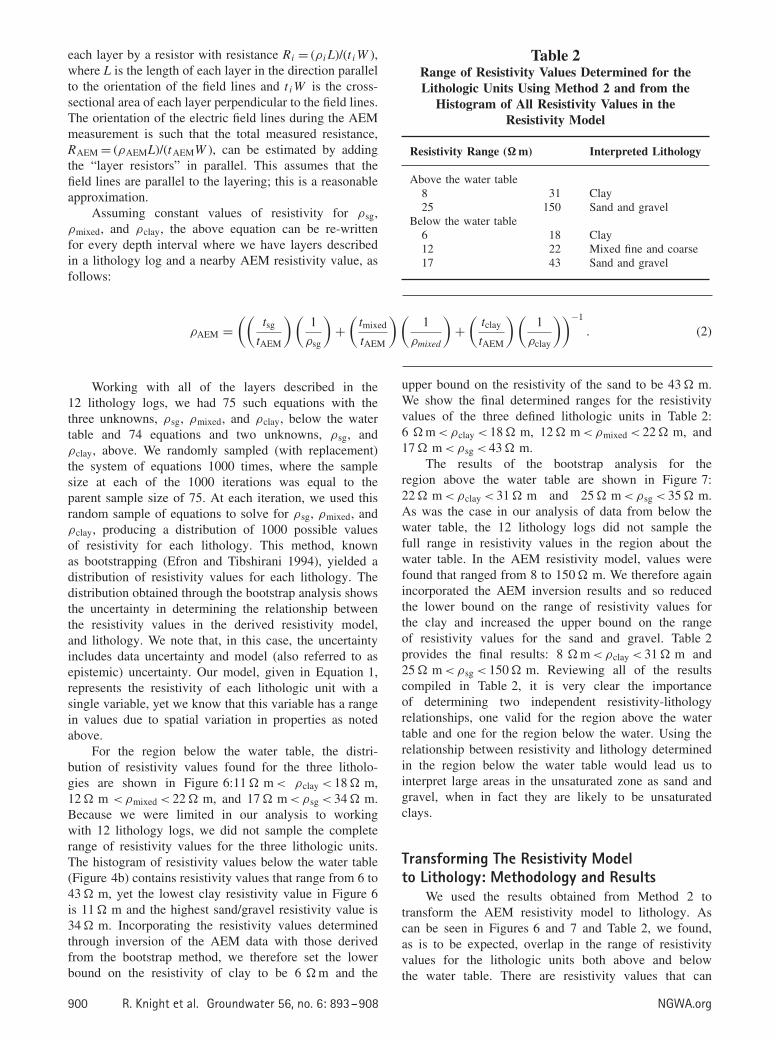
Working with all of the layers described in the12 lithology logs, we had 75 such equations with thethree unknowns, ρsg, ρmixed, and ρclay, below the watertable and 74 equations and two unknowns, ρsg, andρclay, above. We randomly sampled (with replacement)the system of equations 1000 times, where the samplesize at each of the 1000 iterations was equal to theparent sample size of 75. At each iteration, we used thisrandom sample of equations to solve for ρsg, ρmixed, andρclay, producing a distribution of 1000 possible valuesof resistivity for each lithology. This method, knownas bootstrapping (Efron and Tibshirani 1994), yielded adistribution of resistivity values for each lithology. Thedistribution obtained through the bootstrap analysis showsthe uncertainty in determining the relationship betweenthe resistivity values in the derived resistivity model,and lithology. We note that, in this case, the uncertaintyincludes data uncertainty and model (also referred to asepistemic) uncertainty. Our model, given in Equation 1,represents the resistivity of each lithologic unit with asingle variable, yet we know that this variable has a rangein values due to spatial variation in properties as notedabove.

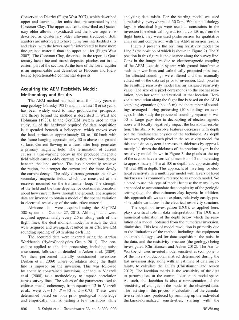
For the region below the water table, the distri-bution of resistivity values found for the three litholo-gies are shown in Figure 6:11 � m < ρclay < 18 � m,12 � m <ρmixed < 22 � m, and 17 � m < ρsg < 34 � m.Because we were limited in our analysis to workingwith 12 lithology logs, we did not sample the completerange of resistivity values for the three lithologic units.The histogram of resistivity values below the water table(Figure 4b) contains resistivity values that range from 6 to43 � m, yet the lowest clay resistivity value in Figure 6is 11 � m and the highest sand/gravel resistivity value is34 � m. Incorporating the resistivity values determinedthrough inversion of the AEM data with those derivedfrom the bootstrap method, we therefore set the lowerbound on the resistivity of clay to be 6 � m and the

Table 2Range of Resistivity Values Determined for theLithologic Units Using Method 2 and from the

Histogram of All Resistivity Values in theResistivity Model

Resistivity Range (� m) Interpreted Lithology

Above the water table8 31 Clay25 150 Sand and gravel

Below the water table6 18 Clay12 22 Mixed fine and coarse17 43 Sand and gravel

upper bound on the resistivity of the sand to be 43 � m.We show the final determined ranges for the resistivityvalues of the three defined lithologic units in Table 2:6 � m < ρclay < 18 � m, 12 � m < ρmixed < 22 � m, and17 � m < ρsg < 43 � m.

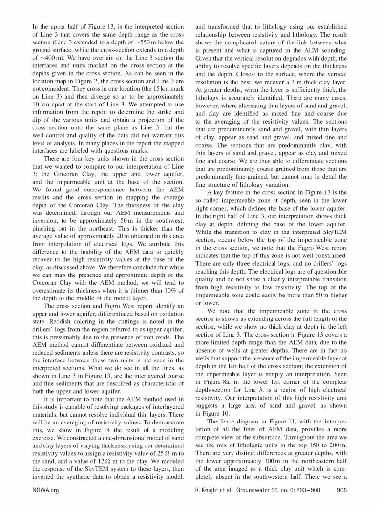
The results of the bootstrap analysis for theregion above the water table are shown in Figure 7:22 � m < ρclay < 31 � m and 25 � m < ρsg < 35 � m.As was the case in our analysis of data from below thewater table, the 12 lithology logs did not sample thefull range in resistivity values in the region about thewater table. In the AEM resistivity model, values werefound that ranged from 8 to 150 � m. We therefore againincorporated the AEM inversion results and so reducedthe lower bound on the range of resistivity values forthe clay and increased the upper bound on the rangeof resistivity values for the sand and gravel. Table 2provides the final results: 8 � m < ρclay < 31 � m and25 � m < ρsg < 150 � m. Reviewing all of the resultscompiled in Table 2, it is very clear the importanceof determining two independent resistivity-lithologyrelationships, one valid for the region above the watertable and one for the region below the water. Using therelationship between resistivity and lithology determinedin the region below the water table would lead us tointerpret large areas in the unsaturated zone as sand andgravel, when in fact they are likely to be unsaturatedclays.

Transforming The Resistivity Modelto Lithology: Methodology and Results

We used the results obtained from Method 2 totransform the AEM resistivity model to lithology. Ascan be seen in Figures 6 and 7 and Table 2, we found,as is to be expected, overlap in the range of resistivityvalues for the lithologic units both above and belowthe water table. There are resistivity values that can

900 R. Knight et al. Groundwater 56, no. 6: 893–908 NGWA.org

20 25 30 35

resistivity, ohm-m

0

50

100

150

200

250

300

coun

tclay

sand & gravel

Figure 7. Resistivity values determined for clay, sand, andgravel in the region above the water table using Method2. These values were obtained with a bootstrap analysisusing all depth intervals above the water table in the 12lithology logs and corresponding resistivity values from theAEM resistivity model.

be interpreted, with a high degree of confidence, tobe a specific lithology. For example, above the watertable, ρAEM > 31 � m can be defined as an unsaturatedsand and gravel, and ρAEM < 25 � m can be defined asclay, but for measured resistivity values in the range25 � m ≤ ρAEM ≤ 31 � m we cannot determine whetherthe lithology is clay or sand and gravel. Beneath thewater table similar uncertainty exists. We can interpretas sand and gravel those areas where ρAEM > 22 � m,and interpret as clay those areas where ρAEM < 12 � m,but there are areas where uncertainty exists in terms ofdefining lithology. We elected to honor this uncertaintyby displaying in Figure 8a and 8b the results in termsof the AEM resistivity values, showing on the color barthe correspondence between resistivity and lithology inthe regions above and below the water table, using thetwo independent resistivity-lithology relationships that wehave defined. We note that in displaying the data we haveelected to bin all resistivity values above 50 � m (whichincludes only 2% of the data) so as to expand the colorbar. Figure 8a shows the results from Line 3 (locationin Figure 2); Figure 8b is a fence diagram displayingall of the AEM survey results. We interpret, and labelin Figure 8a, the relatively thick, continuous conductivelayer at approximately 100 m depth on the left side of thesection to be the Corcoran Clay; the conductive featurethins and terminates on the right side of the section. TheCorcoran Clay is known, from drillers’ logs, to be present

at this depth in this area, becoming discontinuous in thenortheast (the right side of Figure 8a).

In addition to this presentation of the results we alsotransformed the resistivity model to lithology in two otherways that communicate information about the lithologicvariation in the subsurface mapped with the AEM method.The three images in Figure 9 display the probabilityof sand and gravel (Figure 9a), mixed fine and coarse(Figure 9b), and clay (Figure 9c) at any given location.We created these images by taking the distributions shownin Figures 6 and 7 as indicative of the probabilities offinding a lithology at a location. The final way in which wedisplay our results is given in Figure 10, which shows themost probable lithology at any location along Line 3 as asingle profile plot, and Figure 11, which displays the fullinterpreted data set as a fence diagram. The conductivefeature labeled in Figure 8a as Corcoran Clay, appearsas the thick clay unit in Figures 10 and 11, at a depthof approximately 100 m, present in all sections in thesouthwestern part of the study area.

DiscussionThe motivation for this study was to determine

whether the AEM method could be used for mapping theaquifer systems in the Central Valley, recognizing thatthe findings here would have implications for using theAEM method in characterizing other alluvial aquifers.Let us consider the first question we addressed, relatedto the imaging capability of the method: How effectivewould the AEM method be in imaging beneath theshallow, electrically conductive clays commonly found inthe Central Valley? Our concern had been that electricallyconductive clays would limit the DOI. We obtained AEMdata of excellent quality to a depth of approximately 400 malong all of the flight lines. Neither the thick CorcoranClay, nor the numerous fine clay layers described inthe lithology logs, negatively impacted the penetrationdepth of the measurement. The calculation of the DOIsdetermined an upper DOI between 300 and 400 m and thelower DOI at approximately 500 m. Somewhere betweenthe upper and lower DOI’s, and usually deeper thanthe lower DOI, accurate resolution of the true electricalresistivity of the subsurface region being sampled isreduced. At this depth the imaging, through numericalinversion, transitions from accurately resolving the valuesof electrical resistivity to detecting changes in theelectrical resistivity. Note that while detection indicatesthat the true magnitude of the electrical resistivity maynot be accurately resolved; there is still some sensitivityto changes. Somewhere deeper than the lower DOI isgenerally the line of demarcation between resolution anddetection. It is different in every data set due to differencesin data noise and the electrical resistivity structure. Thelower DOI is usually taken as a depth to which there isvery high confidence in the resolved resistivity values.The lower DOI usually represents a depth at which thetransition occurs from resolution to detection.

NGWA.org R. Knight et al. Groundwater 56, no. 6: 893–908 901

(a)

(b)

Figure 8. Resistivity model with interpreted lithology for (a) data acquired along Line 3, which runs from the southwest (leftside of figure) to the northeast, and (b) all acquired data as a fence diagram. As shown in Figure 2, the long lines in the fencediagram in (b) run from the southwest (lower left corner) to the northeast (upper right corner).

As an example of applying the concept of DOI indetermining the level of confidence in a resistivity model,consider the high resistivity unit seen in Figure 8a on thesouthwestern end of Line 3 and in the fence diagram inFigure 8b. This unit falls between the upper DOI (thedotted line) and the lower DOI, approximately coincidingwith the base of the displayed model. The fact that thehigh resistivity unit begins at approximately the depth ofthe upper DOI does not mean that it should be questionedas a potential geologic unit. Anything below the lowerDOI is in the transition range between resolved anddetected. So while the resistivity of the high resistivity unitmight not be accurately determined (i.e., the resistivitymight not be exactly 40 � m) below the lower DOI, it willhave a detected range of approximately 30 to 60 � m; thisprovides a high level of confidence in its identification asa high resistivity unit. The finding in this study, that wecan accurately resolve the resistivity model to a depth ofapproximately 500 m and detect changes in resistivity togreater depths, is an important result for evaluating andplanning AEM surveys for subsurface mapping in otherparts of the Central Valley.

In addition to determining to what depth we canresolve/detect changes in resistivity, it is also importantto consider how well we can capture vertical changesin resistivity and the implications for estimating thethicknesses of various units. The Corcoran Clay is themain confining unit between the upper and lower portions

of the aquifer system, and can be seen in the resistivitysections in Figure 8 and in the interpreted sections inFigures 10 and 11. In order to determine how accuratelythe AEM method can determine the thickness of theCorcoran Clay, we generated a simple model of theelectrical resistivity variation across the clay, and thenmodeled the response of the SkyTEM system and invertedthe data, to compare the inverted clay thickness to the“true” clay thickness.

In Figure 12 we show, as the red line, a simplifiedrepresentation of the true electrical resistivity variationacross the Corcoran Clay, using as “true” the resistivityvalues from an electrical log for well 20S23E14, which islocated about 300 m from the flight lines. Above, below,and within the Corcoran Clay, we set the resistivity toconstant values, equal to the average values seen in thesezones in the electrical log. We generated synthetic AEMdata by modeling the response of the SkyTEM 508 systemto the variation in resistivity values. We then invertedthe synthetic data, using the same inversion process aswas applied to the full data set in this study, so that thelayer thickness was set to 3 m at the surface and thenincreased by 10% with depth (so that each layer thicknesswas 1.1 times that of the previous layer). This yieldedthe resistivity variation that would be seen in the AEMresistivity model, shown as the blue line in Figure 12.

While the inverted resistivity values in Figure 12 donot perfectly match the true resistivity values, they do

902 R. Knight et al. Groundwater 56, no. 6: 893–908 NGWA.org

(a)

(b)

(c)

Figure 9. Probability, based on distributions from Method 2 bootstrap results, of the occurrence along Line 3 of: (a) sandand gravel, (b) mixed fine and coarse, and (c) clay.

Figure 10. Most probable lithology along Line 3, based on distributions from Method 2 bootstrap results.

capture the general trend, with the Corcoran Clay clearlyimaged as being conductive. The basic guideline forelectromagnetic modeling is that there will be sensitivityto a layer whose thickness is at least 10% of the depthto the layer. The resistivity values may not be highlyaccurate, but there will be evidence that a conductive zoneis present.

It is important to note the smoothing seen inthe inversion result that masks the abrupt changes inresistivity. There are constraints in the inversion routine,on the allowed change in resistivity between adjacentlayers, so that the inverted AEM data show a more gradualchange in resistivity than is present. As a result, theinverted Corcoran Clay thickness is greater than the truethickness. This is likely to be a general result, suggestingthat in all of our sections displaying the interpretedvariation in lithology, the thickness of the Corcoran Clay

will be overestimated if it is thinner than 10% of thedepth to the middle of the layer in which it is indicated.Sharper vertical boundaries in the resistivity models couldbe achieved with different inversion strategies such as theminimum gradient support or with a few-layered inversionthat solves for the resistivity and thickness of each layer(Vignoli et al. 2017). Adding a-priori information to theinversion could also improve the accuracy of the spatialextent of the recovered conductive layer (e.g., Sapia et al.2014).

Once a resistivity model was obtained, we addressedthe second question: Could we use the resistivity modelsand the limited well data to obtain information about thearchitecture of the aquifer systems, mapping out large-scale hydrostratigraphic packages? The first step involvestransforming the resistivity values to lithology. We usedtwo methods. Method 1 is an established approach that

NGWA.org R. Knight et al. Groundwater 56, no. 6: 893–908 903

Figure 11. Fence diagram showing interpretation of all lines of acquired AEM data, displaying the most probable lithologyat each location.

Figure 12. Variation in electrical resistivity across the Cor-coran Clay. The true values were assigned using averagevalues from an electrical log for a well located about 300 mfrom the AEM lines. The inverted values were obtained bymodeling the response of the SkyTEM system to the trueresistivity variation, and then inverting the synthetic data.

provided us with a range of resistivity values for eachlithology. Method 2 was designed to specifically linkthe SkyTEM-measured resistivity to lithology. As part ofthis method, we further refined the range of values byseparating the region above and below the water table andusing a bootstrapping method to obtain the distribution ofresistivity values for each lithology.

Comparing first the resistivity range determined forthe sands and gravels, we find that both methods gavevery similar results, with the total range from Method 1being 19 to 150 � m, and from Method 2 being 17 to150 � m. The resistivity range found for clay below thewater table with Method 2 (6 to 18 � m) includes close tothe full range of values found for clay, silty clay, clayey

silt, interbedded sand/clay/silt with Method 1, a veryreasonable result, again indicating very good agreementbetween the two approaches. Higher resistivity valueswere found for clay above the water table using Method2—resistivity values as high as 31 � m. In Method 2we defined a category “mixed fine and coarse” belowthe water table, finding resistivity values that overlappedwith those for clay and sands/gravels. We conclude thatMethod 2 provided us with resistivity values that agreewell with those determined using the established approachof Method 1; and provided further information about theimpact of saturation state (above or below the water table)on transforming resistivity values to lithology.

An important feature in the use of Method 2 is theability to capture a distribution of resistivity values foreach lithology. This allowed us to display the probabilityof the occurrence of each lithology (Figure 9) and our“best guess” (Figures 10 and 11) that transforms eachresistivity value to the lithology most likely to occur.Working with distributions and providing a lithologicinterpretation in terms of probabilities of occurrence isa first step towards capturing and communicating to end-users uncertainty in the interpretation of AEM data. Arecent paper used the dataset presented here to developnew ways to use color wheels to display this uncertainty(Nordin et al. 2016).

Let us now consider whether the resulting variationin lithology, derived from the AEM resistivity models,allowed us to map out the large-scale hydrostratigraphy.We compare our results to a cross section in the areaof the flight lines, provided by the Kaweah Delta WaterConservation District (Fugro West 2007). A simplifiedversion of the portion of the cross-section closest toour flight lines (B-B′ in the referenced report), labeledaccording to the interpretation in the report, is providedin the lower half of Figure 13; the location of this portionof the cross section is shown in Figure 2, labeled A-A′.

904 R. Knight et al. Groundwater 56, no. 6: 893–908 NGWA.org

In the upper half of Figure 13, is the interpreted sectionof Line 3 that covers the same depth range as the crosssection (Line 3 extended to a depth of ∼550 m below theground surface, while the cross-section extends to a depthof ∼400 m). We have overlain on the Line 3 section theinterfaces and units marked on the cross section at thedepths given in the cross section. As can be seen in thelocation map in Figure 2, the cross section and Line 3 arenot coincident. They cross in one location (the 15 km markon Line 3) and then diverge so as to be approximately10 km apart at the start of Line 3. We attempted to useinformation from the report to determine the strike anddip of the various units and obtain a projection of thecross section onto the same plane as Line 3, but thewell control and quality of the data did not warrant thislevel of analysis. In many places in the report the mappedinterfaces are labeled with questions marks.

There are four key units shown in the cross sectionthat we wanted to compare to our interpretation of Line3: the Corcoran Clay, the upper and lower aquifer,and the impermeable unit at the base of the section.We found good correspondence between the AEMresults and the cross section in mapping the averagedepth of the Corcoran Clay. The thickness of the claywas determined, through our AEM measurements andinversion, to be approximately 50 m in the southwest,pinching out in the northeast. This is thicker than theaverage value of approximately 20 m obtained in this areafrom interpolation of electrical logs. We attribute thisdifference to the inability of the AEM data to quicklyrecover to the high resistivity values at the base of theclay, as discussed above. We therefore conclude that whilewe can map the presence and approximate depth of theCorcoran Clay with the AEM method, we will tend tooverestimate its thickness when it is thinner than 10% ofthe depth to the middle of the model layer.

The cross section and Fugro West report identify anupper and lower aquifer, differentiated based on oxidationstate. Reddish coloring in the cuttings is noted in thedrillers’ logs from the region referred to as upper aquifer;this is presumably due to the presence of iron oxide. TheAEM method cannot differentiate between oxidized andreduced sediments unless there are resistivity contrasts, sothe interface between these two units is not seen in theinterpreted sections. What we do see in all the lines, asshown in Line 3 in Figure 13, are the interlayered coarseand fine sediments that are described as characteristic ofboth the upper and lower aquifer.

It is important to note that the AEM method used inthis study is capable of resolving packages of interlayeredmaterials, but cannot resolve individual thin layers. Therewill be an averaging of resistivity values. To demonstratethis, we show in Figure 14 the result of a modelingexercise. We constructed a one-dimensional model of sandand clay layers of varying thickness, using our determinedresistivity values to assign a resistivity value of 25 � m tothe sand, and a value of 12 � m to the clay. We modeledthe response of the SkyTEM system to these layers, theninverted the synthetic data to obtain a resistivity model,

and transformed that to lithology using our establishedrelationship between resistivity and lithology. The resultshows the complicated nature of the link between whatis present and what is captured in the AEM sounding.Given that the vertical resolution degrades with depth, theability to resolve specific layers depends on the thicknessand the depth. Closest to the surface, where the verticalresolution is the best, we recover a 3 m thick clay layer.At greater depths, when the layer is sufficiently thick, thelithology is accurately identified. There are many cases,however, where alternating thin layers of sand and gravel,and clay are identified as mixed fine and coarse dueto the averaging of the resistivity values. The sectionsthat are predominantly sand and gravel, with thin layersof clay, appear as sand and gravel, and mixed fine andcoarse. The sections that are predominantly clay, withthin layers of sand and gravel, appear as clay and mixedfine and coarse. We are thus able to differentiate sectionsthat are predominantly coarse-grained from those that arepredominantly fine-grained, but cannot map in detail thefine structure of lithology variation.

A key feature in the cross section in Figure 13 is theso-called impermeable zone at depth, seen in the lowerright corner, which defines the base of the lower aquifer.In the right half of Line 3, our interpretation shows thickclay at depth, defining the base of the lower aquifer.While the transition to clay in the interpreted SkyTEMsection, occurs below the top of the impermeable zonein the cross section, we note that the Fugro West reportindicates that the top of this zone is not well constrained.There are only three electrical logs, and no drillers’ logsreaching this depth. The electrical logs are of questionablequality and do not show a clearly interpretable transitionfrom high resistivity to low resistivity. The top of theimpermeable zone could easily be more than 50 m higheror lower.

We note that the impermeable zone in the crosssection is shown as extending across the full length of thesection, while we show no thick clay at depth in the leftsection of Line 3. The cross section in Figure 13 covers amore limited depth range than the AEM data, due to theabsence of wells at greater depths. There are in fact nowells that support the presence of the impermeable layer atdepth in the left half of the cross section; the extension ofthe impermeable layer is simply an interpretation. Seenin Figure 8a, in the lower left corner of the completedepth-section for Line 3, is a region of high electricalresistivity. Our interpretation of this high resistivity unitsuggests a large area of sand and gravel, as shownin Figure 10.

The fence diagram in Figure 11, with the interpre-tation of all the lines of AEM data, provides a morecomplete view of the subsurface. Throughout the area wesee the mix of lithologic units in the top 150 to 200 m.There are very distinct differences at greater depths, withthe lower approximately 300 m in the northeastern halfof the area imaged as a thick clay unit which is com-pletely absent in the southwestern half. There we see a

NGWA.org R. Knight et al. Groundwater 56, no. 6: 893–908 905

Figure 13. Interpretation of Line 3 above A-A′, the location of which is shown in Figure 2. Note that A-A′ is a portion ofcross section B-B′ from the report by West (2007). The interfaces and units marked on the cross section have been overlainon the Line 3, at the depths shown in the cross section.

(a) (b)

Figure 14. (a) 1D model of alternating layers of sand andgravel, and clay. (b) The simulated AEM sounding obtainedfrom modeling the acquisition, inversion and interpretationof SkyTEM data. The averaging of resistivity values meansthat fine layers are not recovered, and layers are identifiedas mixed fine and coarse.

nearly continuous layer of highly resistive materials inter-preted as sand and gravel. While there are no lithologylogs that reach this depth that could be used to supportthis interpretation, the recent drilling of deep wells in thisarea has reported finding sand and gravel (A. Fukuda,personal communication, 2016). The ability to map thehydrostratigraphy, below the current depth range of wellsin an area, is one obvious benefit of utilizing the AEMmethod to acquire the data needed for improved concep-tual models of aquifer systems. Ongoing research is nowfocused on integrating all well data with the AEM data tobuild a conceptual model for this area, and evaluate the

extent to which incorporating the AEM data enhances theaccuracy and usefulness of the groundwater models usedto support local groundwater management decisions.

The motivation for conducting this study was toassess the value of the AEM method as a cost-effectiveway to map the aquifer systems of the Central Valley.In terms of mapping the aquifer systems, wells are anestablished method and can provide detailed information,at one location. While the vertical resolution of AEMdata can never match that of a well, even abundant welldata yield little information in the horizontal directions,where difficult to identify features such as windowsthrough aquitards and coarse-grained channel depositscan radically change groundwater flow and transportvelocities. There is considerable value in mapping outthe large-scale hydrostratigraphy and the under-sampled,lateral variations in aquifer system properties with theAEM method. In addition, the many wells that have beendrilled in the Central Valley tend to be shallow, so do notprovide information about the deeper parts of the aquifersystem. It is important to acknowledge, however, that thepresence of wells is a necessary part of the analysis andinterpretation of AEM data; but even with sparse welldata, as was the case in this study, valuable informationabout the subsurface hydrostratigraphy can be obtainedfrom the AEM data.

In terms of the costs of acquiring subsurface data,wells can be expensive to drill, especially deeper wells,with the cost of a monitoring well typically exceeding$100,000. A conservative estimate of the cost of an AEMsurvey, for data acquisition, analysis and interpretationis $450 per line km, with an additional approximately$20,000 for mobilization and demobilization of thesystem. A ground-based geophysical method could beemployed at a few locations for less than the cost ofmobilization of the AEM system. But the coverage thatcan be obtained with the AEM method could not beachieved with any other method for similar costs. Giventhe cost of drilling wells, especially monitoring wells, itcould therefore be highly cost-effective to use AEM datato obtain a large-scale image of an area, and then usethe results to guide the selection of drilling locations. The

906 R. Knight et al. Groundwater 56, no. 6: 893–908 NGWA.org

complementary use of well data and geophysical data,where each has its costs and benefits, is an effectiveapproach to obtaining the information required to supportthe management of groundwater resources.

ConclusionsThis study has allowed us to assess the viability of

using the AEM method to map the aquifer systems of theCentral Valley; and, more generally, to map similar aquifersystems in sedimentary basins containing significant fines.We conclude that the regional implementation of theAEM method could provide critical information aboutthe hydrostratigraphy of the aquifer systems needed forgroundwater management. What we were able to derivefrom the AEM data about the large-scale structure, farexceeds what is possible using traditional methods basedon the drilling of wells.

We found it possible to image the electrical resistivityto a depth of approximately 500 m; given the geology ofthe Central Valley we would expect to find similar imagingdepths at most other locations throughout the valley. Thiscovers the relevant depth range for current groundwatermanagement and provides information about the deeperregions of the aquifer system not currently sampled bywells. In addition, the lateral spatial resolution seen in theAEM data could never be obtained with well data, and isneeded to reveal the large-scale heterogeneity that shouldbe captured in groundwater models.

We developed a new methodology to transformthe resistivity model to lithology which can be appliedthroughout the Central Valley, and could be widelyadopted as a new approach to the interpretation of AEMdata. The key limitation in this approach will alwaysbe the shallow depth of most of the lithology logs,resulting in a resistivity-lithology relationship that isestablished and thus valid at shallow depths, but onlyassumed to be valid at greater depths. We are currentlyexploring ways to correct for the effect of depth onthis relationship. The approach yields a distribution ofresistivity values, positioning us to be able to quantifyand account for this source of uncertainty in using theAEM data to generate conceptual models. Our resultinginterpretation of lithology was consistent with otherlithologic information from the area, while noting thatthe vertical resolution of the AEM method resulted in anoverestimation of the thickness of the Corcoran Clay unitand an inability to detect relatively thin layers at depth.

AEM imaging to depths of approximately 500 m canprovide critical information about the distribution andconnectivity of hydrostratigraphic packages that wouldsupport the development of conceptual models and wouldreveal permeable pathways that could be used to rechargegroundwater at shallow and deeper levels. The acquiredinformation would directly support specific managementactions such as the selection of sites for surface spreadingrecharge, and the siting of monitoring wells. In this studywe used the SkyTEM 508 system as we were interestedin maximizing the depth of imaging while maintaining

reasonably high resolution in the top approximately100 m. If the goal in a project were to more accuratelyresolve the top 50 to 100 m to assess recharge potential,other AEM systems could be used.

This study was motivated by our interest in exploringthe use of the AEM method to address the critical need forsubsurface data, in order to implement new groundwaterlegislation in California. We conclude that the acquisitionof AEM data throughout the Central Valley would providethe hydrogeological framework needed to support theestablishment of sustainable groundwater management inCalifornia.

AcknowledgmentsWe would like to thank Paul Hendrix and Aaron

Fukuda from the Tulare Irrigation District, Noah Dewarfrom Stanford University, and Franklin Koch and AdamPidlisecky from Seequent. We also wish to thank thethree anonymous reviewers for their helpful comments.Funding sources include the School of Earth, Energyand Environmental Sciences at Stanford University, theNational Science Foundation (graduate fellowship grantnumber DGE-114747) and the UC Office of the Presi-dent’s Multi-Campus Research Programs and Initiatives(MR-15-328473) through UC Water, the University ofCalifornia Water Security and Sustainability ResearchInitiative.

Authors’ NoteThe authors do not have any conflicts of interest.

ReferencesAuken, E., A.V. Christiansen, J.H. Westergaard, C. Kirkegaard,

N. Foged, and A. Viezzoli. 2009. An integrated processingscheme for high resolution airborne electromagnetic sur-veys, the SkyTEM system. Exploration Geophysics 40, no.2: 184–192.

Barfod, A.A., I. Møller, and A.V. Christiansen. 2016. Compilinga national resistivity atlas of Denmark based on airborneand ground-based transient electromagnetic data. Journalof Applied Geophysics 134: 199–209.

Bedrosian, P.A., C. Schamper, and E. Auken. 2015. A com-parison of helicopter-borne electromagnetic systems forhydrogeological studies. Geophysical Prospecting 64, no.1: 192–215.

Berardino, P., G. Fornaro, R. Lanari, and E. Sansosti. 2002. Anew algorithm for surface deformation monitoring basedon small baseline differential SAR interferograms. IEEETransactions on Geoscience and Remote Sensing 40, no.11: 2375–2383.

California Department of Water Resources. 2003. Califor-nia’s groundwater. Bulletin 118, update 2003. http://www.water.ca.gov/groundwater/bulletin118/index.cfm (accessedJune 1, 2017).

Christensen, N.K., B.J. Minsley, and S. Christensen. 2017.Generation of 3-D hydrostratigraphic zones from denseairborne electromagnetic data to assess groundwater modelprediction error. Water Resources Research 53: 1019–1038.

NGWA.org R. Knight et al. Groundwater 56, no. 6: 893–908 907

Christiansen, A.V., N. Foged, and E. Auken. 2014. A concept forcalculating accumulated clay thickness from borehole litho-logical logs and resistivity models for nitrate vulnerabilityassessment. Journal of Applied Geophysics 108: 69–77.

Christiansen, A.V., and E. Auken. 2012. A global mea-sure for depth of investigation. Geophysics 77, no. 4:WB171–WB177.

Efron, B., and R.J. Tibshirani. 1994. An Introduction to theBootstrap. Boca Raton, Florida: CRC Press.

Farr, T.G., and Z. Liu. 2014. Monitoring subsidence associatedwith groundwater dynamics in the Central Valley ofCalifornia using interferometric radar. Remote Sensing ofthe Terrestrial Water Cycle 206: 397.

Faunt, C.C., and M. Sneed. 2015. Water availability andsubsidence in California’s Central Valley. San FranciscoEstuary and Watershed Science 13, no. 3: 3.

Fugro West. 2007. Water resources investigation of the KaweahDelta Water Conservation District. Technical report pre-pared for Kaweah Delta Water Conservation District,Project 3087.004.07. http://www.kdwcd.com/wri-report__2007__condensed_version.pdf (accessed June 1, 2017).

Høyer, A.S., F. Jørgensen, P.B.E. Sandersen, A. Viezzoli, andI. Møller. 2015. 3D geological modelling of a complexburied-valley network delineated from borehole and AEMdata. Journal of Applied Geophysics 122: 94–102.

HydroGeophysics Group. 2011. Guide for processing andinversion of SkyTEM data in Aarhus Workbench, Version2.0. HydroGeophysics Group, Aarhus University. http://www.hgg.geo.au.dk/rapporter/guide_skytem_proc_inv.pdf(accessed January 1, 2017).

Jørgensen, F., R.R. Møller, L. Nebel, N.P. Jensen, A.V.Christiansen, and P.B. Sandersen. 2013. A method forcognitive 3D voxel modeling of AEM data. Bulletin ofEngineering Geology and the Environment 72, no. 3–4:421–432.

Jørgensen, F., P.B. Sandersen, and E. Auken. 2003. Imagingburied quaternary valleys using the transient electromag-netic method. Journal of Applied Geophysics 53, no. 4:199–213.

Knight, R., and A.L. Endres. 2005. An introduction to rockphysics for near-surface applications in near-surface geo-physics. Volume 1: Concepts and fundamentals. In NearSurface Geophysics , ed. D. Butler, 31–70. Tulsa, Okla-homa: Society of Exploration Geophysicists.

Madsen, S.N., and H.A. Zebker. 1998, 1998. Imaging radarinterferometry, ch. 6. In Principles and Applications ofImaging Radar . Manual of Remote Sensing, Vol. 2, ed.F.M. Henderson and A.J. Lewis, 359, 866–380. New York:Wiley.

Marker, P.A., N. Foged, X. He, A.V. Christiansen, J.C. Ref-sgaard, E. Auken, and P. Bauer-Gottwein. 2015. Perfor-mance evaluation of groundwater model hydrostratigraphyfrom airborne electromagnetic data and lithological bore-hole logs. Hydrology and Earth System Sciences 19, no. 9:3875–3890.

Møller, I., V.H. Søndergaard, F. Jørgensen, E. Auken, and A.V.Christiansen. 2009. Integrated management and utilizationof hydrogeophysical data on a national scale. Near SurfaceGeophysics 7, no. 5–6: 647–659.

Nordin, M., R. Smith, and R. Knight. 2016. The use of colorwheels to communicate uncertainty in the interpretation ofgeophysical data. The Leading Edge 35, no. 9: 786–789.

Palacky, G.J. 1981. The airborne electromagnetic method as atool of geological mapping. Geophysical Prospecting 29,no. 1: 60–88.

Podgorski, J.E., E. Auken, C. Schamper, A. Vest Christiansen, T.Kalscheuer, and A.G. Green. 2013. Processing and inver-sion of commercial helicopter time-domain electromagneticdata for environmental assessments and geologic and hydro-logic mapping. Geophysics 78, no. 4: E149–E159. https://doi.org/10.1190/geo2012-0452.1

Rosen, P.A., S. Hensley, I.R. Joughin, F.K. Li, S. Madsen, E.Rodriguez, and R.M. Goldstein. 2000. Synthetic apertureradar interferometry. Proceedings of the IEEE 88, no. 3:333–382.

Sapia, V., G.A. Oldenborger, A. Viezzoli, and M. Marchetti.2014. Incorporating ancillary data into the inversion ofairborne time-domain electromagnetic data for hydrogeo-logical applications. Journal of Applied Geophysics 104:35–43.

Sattel, D., and L. Kgotlhang. 2004. Groundwater explorationwith AEM in the Boteti area, Botswana. ExplorationGeophysics 35, no. 2: 147–156.

Smith, R.G., R. Knight, J. Chen, J.A. Reeves, H.A. Zebker,T. Farr, and Z. Liu. 2017. Estimating the permanentloss of groundwater storage in the southern San JoaquinValley, California. Water Resources Research 53, no. 3:2133–2148.

Sørensen, K.I., and E. Auken. 2004. SkyTEM—a new high-resolution helicopter transient electromagnetic system.Exploration Geophysics 35, no. 3: 191–199.

The Nature Conservancy. 2016. Groundwater and stream interac-tion in California’s Central Valley: Insights for sustainablegroundwater management. http://scienceforconservation.org/dl/GroundwaterStreamInteraction_2016.pdf (accessed July1, 2017).

Thomsen, R., V.H. Søndergaard, and K.I. Sørensen. 2004.Hydrogeological mapping as a basis for establishingsite-specific groundwater protection zones in Denmark.Hydrogeology Journal 12, no. 5: 550–562.

U.S. Geological Survey. 2016. California water science cen-ter: California’s Central Valley. https://ca.water.usgs.gov/projects/central-valley/about-central-valley.html (accessedJune 1, 2017).

Viezzoli, A., A.V. Christiansen, E. Auken, and K.I. Sørensen.2008. Quasi-3D modeling of airborne TEM data byspatially constrained inversion. Geophysics 73, no. 3:F105–F113.

Vignoli, G., V. Sapia, A. Menghini, and A. Viezzoli. 2017.Examples of improved inversion of different airborneelectromagnetic datasets via sharp regularization. Journalof Environmental & Engineering Geophysics 22, no. 1:51–61.

Ward, S.H., and G.W. Hohmann. 1988. Electromagnetic theoryfor geophysical applications, ch. 4. In ElectromagneticMethods in Applied Geophysics , ed. M.N. Nabighian. Tulsa,Oklahoma: Society of Exploration Geophysicists.

908 R. Knight et al. Groundwater 56, no. 6: 893–908 NGWA.org