Instructions for use

Title A three-dimensional Resistivity Structure Study Using Airborne Electromagnetics : Application to GREATEM FieldSurvey Data

Author(s) Abdallah, Sabry Abdelmohsen Mohammed

Issue Date 2014-09-25

DOI 10.14943/doctoral.k11538

Doc URL http://hdl.handle.net/2115/57151

Type theses (doctoral)

File Information Abdallah_Sabry_Abdelmohsen_Mohammed.pdf

Hokkaido University Collection of Scholarly and Academic Papers : HUSCAP

二

A three-dimensional Resistivity Structure Study

Using Airborne Electromagnetics: Application

to GREATEM Field Survey Data.

By

Abdallah Sabry Abdelmohsen Mohammed

Submitted for the Degree of Doctor of Philosophy

Dept. Natural History Science,

Graduate school of Science, Hokkaido University

August, 2014

I

ABSTRACT Applications of airborne electromagnetic (AEM) survey techniques have been

introduced for environmental protection and natural disaster prevention in various fields.

The objective of this study was to establish a method of constructing a three-dimensional

(3-D) subsurface electrical resistivity model for a complicated structure using AEM data.

Numerical forward modeling was performed using a modified staggered-grid finite-

difference (SFD) method, and adding a finite-length electrical-dipole (FED) source

routine to generate 3-D resistivity structure models of grounded electrical-source

airborne transient electromagnetic (GREATEM) field survey data.

The GREATEM system was introduced by Mogi et al. (1998, 2009) and uses a

grounded electrical dipole source of 2- to 3-km length as a transmitter and a three-

component magnetometer in the towed bird as a detector. With a grounded source, a

large-moment source can be applied and a long transmitter-receiver distance can be used

to yield a greater depth of investigation, although the survey area becomes limited. Other

advantages include a smaller effect of flight altitude and the possibility of higher-altitude

measurements. Data are recorded in the time domain, providing a raw time series of the

magnetic fields induced by eddy currents in the ground after cutting off the transmitting

current, with the result that a noise filter can be easily introduced.

I have verified our 3-D electromagnetic (EM) modeling computing scheme, which is

based on the SFD method (Fomenko and Mogi, 2002) by comparing the results of a

quarter-space and trapezoidal hill models with the results of the 2.5-D finite-element

method by Mitsuhata (2000), and the 3-D finite-difference program with the spectral

Lanczos decomposition method developed by Druskin and Knizhnerman (1994). This

method was then used to study the possibility of detecting a conductor under shallower

sea, the effects of sea and topographic features.

A GREATEM survey was performed at Kujukuri beach in central Japan, where an

alluvial plain is dominated by sedimentary rocks and shallow water. A reliable resistivity

structure was obtained at a depth range of 300 to 350 m both on land and offshore, in

areas where low-resistivity structures are dominant. Another GREATEM survey was

performed at a location in northwestern Awaji Island, where granitic rocks and

paleogene sedimentary rocks crop out onshore. Resistivity structures at depths of 1 km

II

onshore and 500 m offshore were revealed by this survey. I performed numerical

forward modeling using a modified SFD method by adding a FED source routine to

generate a 3-D resistivity structure model from GREATEM field survey data at both

Kujukuri beach and the Nojima fault.

Finally, I have confirmed the accuracy of our 3-D forward modeling computing scheme

and evaluated the effects of complicated structures, such as sea or topography, on

GREATEM data. I have used this method to generate a 3-D resistivity model from

GREATEM field survey data acquired at the Kujukuri beach and the Nojima fault. As

for results, I have obtained information regarding seawater invasion area in sedimentary

rocks and a resistivity structure along an active fault. This study indicates that the

GREATEM system can be used for the assessment of natural disaster areas.

III

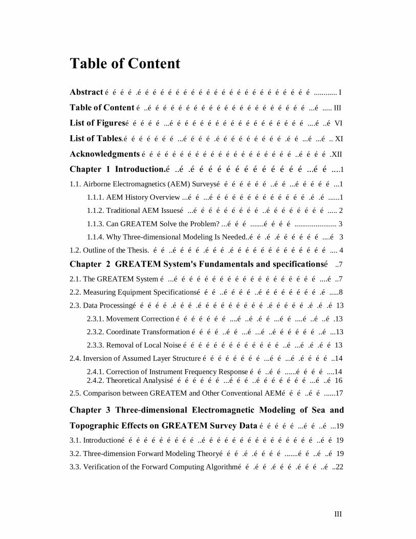
Table of Content Abstract ………….……………………………………………………………............ I

Table of Content …..………………………………………………………...…..... III

List of Figures……………...………………………………………………....…..…VI

List of Tables.…………………...………….……………………….……...…...….. XI

Acknowledgments ……………………………………………………..………….XII

Chapter 1 Introduction.…..….…………………………………...……....1 1.1. Airborne Electromagnetics (AEM) Surveys…………………..……...……………...1

1.1.1. AEM History Overview ...……...………………………………….….…......1

1.1.2. Traditional AEM Issues…...………………………..……………………..... 2

1.1.3. Can GREATEM Solve the Problem? ...……….......…………...................... 3

1.1.4. Why Three-dimensional Modeling Is Needed..…….….………………....… 3

1.2. Outline of the Thesis. ……..………….……….………………………………….... 4

Chapter 2 GREATEM System's Fundamentals and specifications… ..7

2.1. The GREATEM System …...…………………………………………………....…..7

2.2. Measuring Equipment Specifications………..…………..…………………….….....8

2.3. Data Processing…………….……….……………………….…………….….….…13

2.3.1. Movement Correction …………………....…..….……...……....…..…..….13

2.3.2. Coordinate Transformation …………..……...…...…..………………..…...13

2.3.3. Removal of Local Noise …………………………………..…...….….……13

2.4. Inversion of Assumed Layer Structure ……………………...……...….…………..14

2.4.1. Correction of Instrument Frequency Response ……..……......…………....14 2.4.2. Theoretical Analysis…………………...………..…………………...…..…16

2.5. Comparison between GREATEM and Other Conventional AEM………..……......17 Chapter 3 Three-dimensional Electromagnetic Modeling of Sea and

Topographic Effects on GREATEM Survey Data ……………...……..…...19

3.1. Introduction…………………………..………………………………………..……19

3.2. Three-dimension Forward Modeling Theory……….….………….......……..…..…19

3.3. Verification of the Forward Computing Algorithm…….…….……….………..…..22

IV

3.3.1. Quarter-space Model………………………….….……………………..…..22

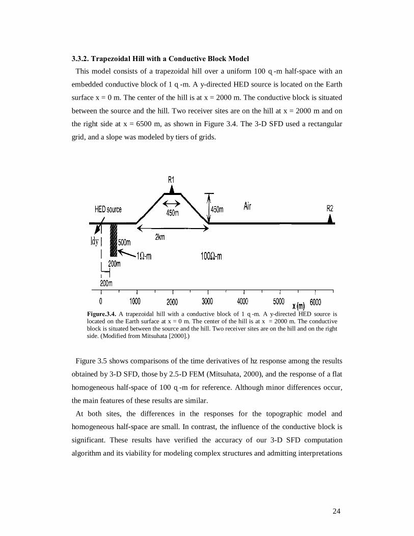
3.3.2. Trapezoidal Hill with a Conductive Block Model………………………….24

3.4. Model Descriptions and Results……...………….………..…………......................25

3.4.1. Sea-land Boundary Model………………………………..…….…….....…...25

3.4.2. Comparison of Sea Effect and the Source Position from Shoreline…..……..26

3.4.3. Comparison of Sea Effect and Host Rock Resistivity..……..…….…..……..29

3.4.4. Topography Model …..…...........................................……………...….….... 31

3.5. Results Summary.......................................................................................................33

3.6. Conclusions………………………….…………………………….………….….... 34

Chapter 4 Three-dimensional Resistivity Modeling of a Coastal Area

Using GREATEM Survey Data from Kujukuri Beach, Chiba, Central

Japan …………………………..……………………………………………….….... 35

4.1. Introduction…….……………………………………………..…………………….35

4.2. Survey Area…………...……………………….…………………………….……. 37

4.3. Data Acquisition ……………..………………….…….…………………….……..39

4.4. Data Processing.………………………………….…………………………..……..39

4.5. One-dimensional Inversion Results…………………...….…………….….…....39

4.6..Three-dimensional Modeling of GREATEM Field Data at Kujukuri

Beach.......................................................................................................................……..40

4.7. Three-dimensional Synthetic Modeling Results ………………….…...…………...43

4.8. Comparison of 1-D and 3-D Resistivity Models……………………………….…..45

4.9. Discussion…………………………...………….…………………………………..47

4.10. Conclusions...………………………………..…………………………..………...49

Chapter 5 Three-dimensional Resistivity Modeling of GREATEM

Survey Data from the Nojima Fault, Awaji Island, Hyogo, Southwest

Japan………………………………………………………………………………......51

5.1. Introduction……………..…………………………………………………………. 51

V

5.2. Survey Area Description…………….…….…...…………………………..……….52

5.3. Previous Geophysical Studies………………..……...………………...…………...52

5.4. Data Acquisition ……………………………....……………...……………………54

5.5. Data Processing……………………...………..………………………….…….…...55

5.6. One-dimensional Inversion Results……………………..….……………...…..…...56

5.7. Three-dimensional Modeling of GREATEM Nojima Field Data………….……....58

5.8. Three-dimensional Synthetic Modeling Results……………….….………….…….59

5.9. Comparison of 1-D and 3-D Resistivity Models …………………………….….....62

5.10. Discussion……………………………………….……………………….………..64

5.11. Conclusions..…………………………...………… …………………….…….......67

Chapter 6 Summary and Future Plans….….....………….……….………...69

List of Related Publications…………….………………………...….…….…….72

References………….…………………..……..……………………….………….…..74

VI

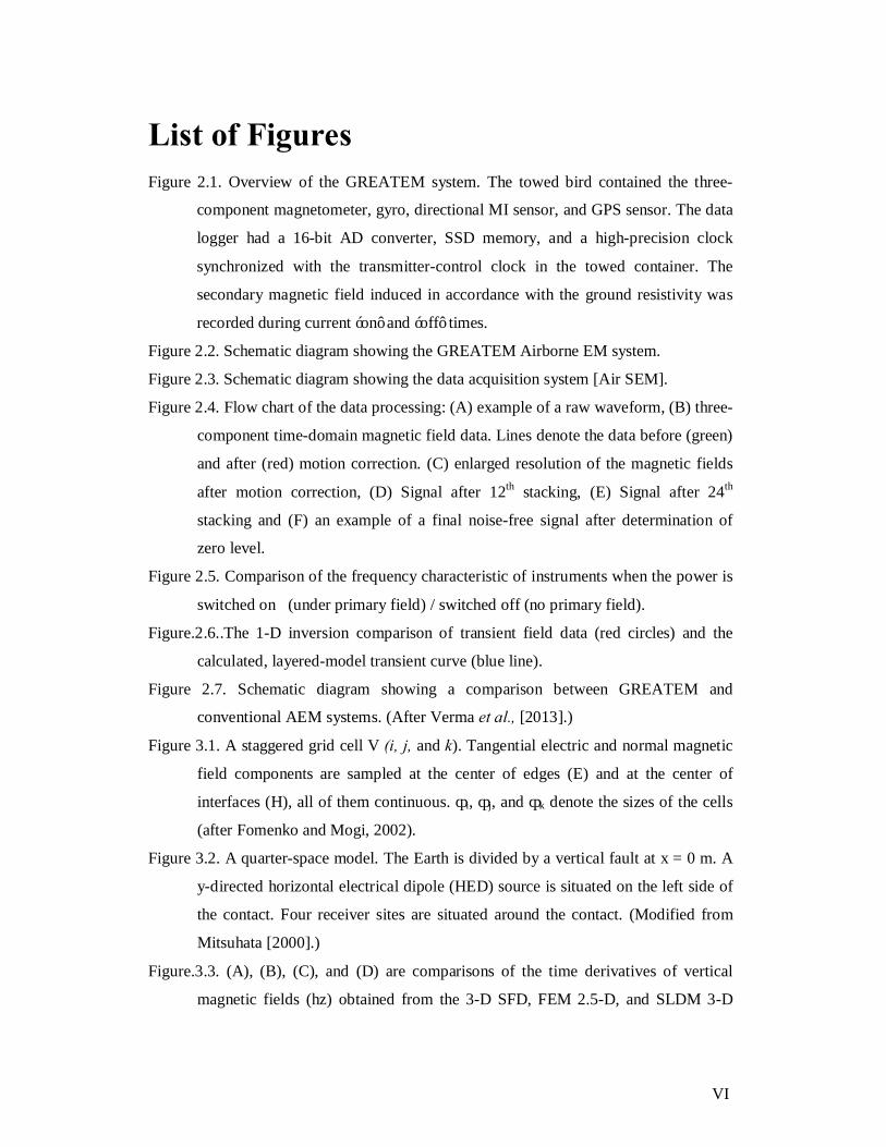
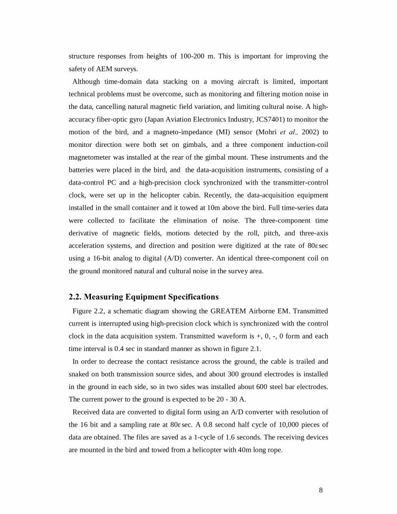
List of Figures Figure 2.1. Overview of the GREATEM system. The towed bird contained the three-

component magnetometer, gyro, directional MI sensor, and GPS sensor. The data

logger had a 16-bit AD converter, SSD memory, and a high-precision clock

synchronized with the transmitter-control clock in the towed container. The

secondary magnetic field induced in accordance with the ground resistivity was

recorded during current ‘on’ and ‘off’ times.

Figure 2.2. Schematic diagram showing the GREATEM Airborne EM system.

Figure 2.3. Schematic diagram showing the data acquisition system [Air SEM].

Figure 2.4. Flow chart of the data processing: (A) example of a raw waveform, (B) three-

component time-domain magnetic field data. Lines denote the data before (green)

and after (red) motion correction. (C) enlarged resolution of the magnetic fields

after motion correction, (D) Signal after 12th stacking, (E) Signal after 24th

stacking and (F) an example of a final noise-free signal after determination of

zero level.

Figure 2.5. Comparison of the frequency characteristic of instruments when the power is

switched on (under primary field) / switched off (no primary field).

Figure.2.6..The 1-D inversion comparison of transient field data (red circles) and the

calculated, layered-model transient curve (blue line).

Figure 2.7. Schematic diagram showing a comparison between GREATEM and

conventional AEM systems. (After Verma et al., [2013].)

Figure 3.1. A staggered grid cell V (i, j, and k). Tangential electric and normal magnetic

field components are sampled at the center of edges (E) and at the center of

interfaces (H), all of them continuous. Δi, Δj, and Δk denote the sizes of the cells

(after Fomenko and Mogi, 2002).

Figure 3.2. A quarter-space model. The Earth is divided by a vertical fault at x = 0 m. A

y-directed horizontal electrical dipole (HED) source is situated on the left side of

the contact. Four receiver sites are situated around the contact. (Modified from

Mitsuhata [2000].)

Figure.3.3. (A), (B), (C), and (D) are comparisons of the time derivatives of vertical

magnetic fields (hz) obtained from the 3-D SFD, FEM 2.5-D, and SLDM 3-D

VII

modeling code for the quarter-space model (Figure 3.2) at the four measuring

points (x = ˗750, ˗250, 250, and 750 m). The analytical solutions for a

homogeneous half-space of 1 Ω-m are shown together. The (+) and (˗) signs

indicate the response. (Modified from Mitsuhata [2000].)

Figure.3.4. A trapezoidal hill with a conductive block of 1 Ω-m. A y-directed HED

source is located on the Earth surface at x = 0 m. The center of the hill is at x =

2000 m. The conductive block is situated between the source and the hill. Two

receiver sites are on the hill and on the right side. (Modified from Mitsuhata

[2000].)

Figure 3.5. Comparisons of the time derivatives of hz obtained from 3-D SFD and FEM

2.5-D modeling code for the trapezoidal hill model of Figure 3.4 with/without a

conductive block. The analytical solutions for a homogeneous half-space of 100

Ω-m are shown together. (Modified from Mitsuhata [2000].)

Figure.3.6. The sea–land boundary model. The sea is a thin layer (10-m depth) with a

resistivity of 0.3 Ω-m placed on top of a uniform half-space Earth medium with a

resistivity of 100 Ω-m. The dipole sources are located 10, 20, and 300 m

landward from the shoreline (x = 0 m).

Figure 3.7. A sketch of the grid cells used for the 3-D EM modeling in this study.

Figure.3.8. (A), (B), and (C) are comparisons of the time derivatives of dhz/dt between

half-space with sea (black)/without sea (blue) for three source positions from the

shoreline (10, 20, and 300 m), respectively (Figure 3.6). (D) Percentage

differences in the responses of dhz/dt for the three cases shown in (A), (B), and

(C).

Figure.3.9. (A), (B), and (C) are comparisons of the time derivatives of hz between half-

space with sea (black)/without sea (blue) in three cases of host rock (100, 10, and

1 Ω-m, respectively). (D) Percentage differences in the dhz/dt response for the

three cases shown in (A, B, and C). The source position is 10 m from the

shoreline.

Figure 3.10. The 3-D topography models. Topography (100 Ω-m) with different slope

angles (α) placed on top of a uniform half-space Earth medium (100 Ω-m).

VIII

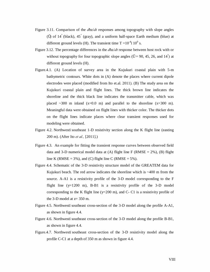
Figure 3.11. Comparison of the dhz/dt responses among topography with slope angles

(α) of 14° (black), 45° (gray), and a uniform half-space Earth medium (blue) at

different ground levels (H). The transient time T =10-4–100 s.

Figure 3.12. The percentage differences in the dhz/dt response between host rock with or

without topography for four topographic slope angles (α = 90, 45, 26, and 14°) at

different ground levels (H).

Figure.4.1. (A) Location of survey area in the Kujukuri coastal plain with 5-m

bathymetric contours. White dots in (A) denote the places where current dipole

electrodes were placed (modified from Ito et.al. 2011). (B) The study area on the

Kujukuri coastal plain and flight lines. The thick brown line indicates the

shoreline and the thick black line indicates the transmitter cable, which was

placed ~300 m inland (x=0.0 m) and parallel to the shoreline (x=300 m).

Meaningful data were obtained on flight lines with thicker color. The thicker dots

on the flight lines indicate places where clear transient responses used for

modeling were obtained.

Figure 4.2. Northwest–southeast 1-D resistivity section along the K flight line (easting

200 m). (After Ito et al., [2011].)

Figure 4.3. An example for fitting the transient response curves between observed field

data and 3-D numerical model data at (A) flight line F (RMSE = 2%), (B) flight

line K (RMSE = 3%), and (C) flight line C (RMSE = 5%).

Figure 4.4. Schematic of the 3-D resistivity structure model of the GREATEM data for

Kujukuri beach. The red arrow indicates the shoreline which is ~400 m from the

source. A-A1 is a resistivity profile of the 3-D model corresponding to the F

flight line (y=1200 m), B-B1 is a resistivity profile of the 3-D model

corresponding to the K flight line (y=200 m), and C- C1 is a resistivity profile of

the 3-D model at z= 350 m.

Figure 4.5. Northwest–southeast cross-section of the 3-D model along the profile A-A1,

as shown in figure 4.4.

Figure 4.6. Northwest–southeast cross-section of the 3-D model along the profile B-B1,

as shown in figure 4.4.

Figure.4.7. Northwest–southeast cross-section of the 3-D resistivity model along the

profile C-C1 at a depth of 350 m as shown in figure 4.4.

IX

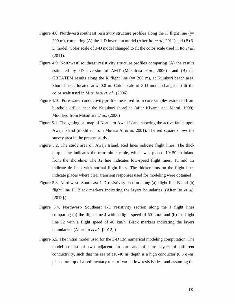
Figure 4.8. Northwest–southeast resistivity structure profiles along the K flight line (y=

200 m), comparing (A) the 1-D inversion model (After Ito et al., 2011) and (B) 3-

D model. Color scale of 3-D model changed to fit the color scale used in Ito et al.,

(2011).

Figure 4.9. Northwest–southeast resistivity structure profiles comparing (A) the results

estimated by 2D inversion of AMT (Mitsuhata et.al., 2006) and (B) the

GREATEM results along the K flight line (y= 200 m), at Kujukuri beach area.

Shore line is located at x=0.0 m. Color scale of 3-D model changed to fit the

color scale used in Mitsuhata et. al., (2006).

Figure 4.10. Pore-water conductivity profile measured from core samples extracted from

borehole drilled near the Kujukuri shoreline (after Kiyama and Marui, 1999).

Modified from Mitsuhata et al., (2006)

Figure 5.1. The geological map of Northern Awaji Island showing the active faults upon

Awaji Island (modified from Murata A. et al. 2001). The red square shows the

survey area in the present study.

Figure 5.2. The study area on Awaji Island. Red lines indicate flight lines. The thick

purple line indicates the transmitter cable, which was placed 10~50 m inland

from the shoreline. The J2 line indicates low-speed flight lines. T1 and T2

indicate tie lines with normal flight lines. The thicker dots on the flight lines

indicate places where clear transient responses used for modeling were obtained.

Figure 5.3. Northwest- Southeast 1-D resistivity section along (a) flight line B and (b)

flight line H. Black markers indicating the layers boundaries. (After Ito et al.,

[2012].)

Figure 5.4. Northwest- Southeast 1-D resistivity section along the J flight lines

comparing (a) the flight line J with a flight speed of 60 km/h and (b) the flight

line J2 with a flight speed of 40 km/h. Black markers indicating the layers

boundaries. (After Ito et al., [2012].)

Figure 5.5. The initial model used for the 3-D EM numerical modeling computation. The

model consist of two adjacent onshore and offshore layers of different

conductivity, such that the sea of (10-40 m) depth is a high conductor (0.3 Ω-m)

placed on top of a sedimentary rock of varied low resistivities, and assuming the

X

presence of topographic structure on the inland side placed on high resistivity

granitic rocks.

Figure 5.6. Examples of fitting the transient response curves between observed field data

and 3-D numerical model data at (A) flight line B (RMSE = 2%), (B) flight line

H (RMSE = 3%), and (C) flight line E (RMSE = 5%).

Figure 5.7. Schematic of the 3-D resistivity structure model from the GREATEM data

for the Nojima fault area. A-A’ is a resistivity profile along the 3-D model

corresponding to the flight line B, B-B’ is a resistivity profile along the 3-D

model corresponding to the flight line H. C-C’, D-D’, E-E’ and F-F’ are

resistivity profiles along the 3-D model for different depth slices at z= 0.0 m

(near surface), 100 m, 300 m and 500 m respectively.

Figure 5.8. Northwest–southeast cross section of the 3-D resistivity model, (a) along A-

A’ profile (Figure 5.7) which corresponding to flight line B and (b) B-B’ profile

(Figure 5.7) which corresponding to flight line H.

Figure 5.9. (A), (B), (C) and (D) are a Plan view of the 3-D resistivity model at different

depth slices along the profiles C-C’, D-D’, E-E’ and F-F’ (Figure 5.7) at different

depth slices at z= 0.0 m (near surface), 100 m, 300 m and 500 m respectively.

Figure.5.10. Northwest-southeast resistivity structure profiles along the B flight line

comparing (A) the 1-D inversion model and (B) 3-D model.

Figure 5.11. Northwest–southeast resistivity structure profiles comparing (A) the results

of CSAMT (Takakura et. al., 1996) and (B) the GREATEM results along the B

flight line at Awaji Island. The black dashed line indicates the Nojima fault.

Color scale of 3-D model changed to fit the color scale used in Takakura et. al.,

(2006).

Figure.5.12. Northwest–southeast resistivity structure profiles comparing (A) the results

of CSAMT (Ikeda et. al., 2000) and (B) the GREATEM results along the B flight

line at Awaji Island. Coast line is at X=0 m. Color scale of 3-D model changed to

fit the color scale used in Ikeda et al. (2000)

Figure.5.13. Resu1ts of the boreho1e e1ectrica1 resistivity 1ogging data obtained from

well drilling close to Nojima fault area. (After Ikeda et al., [2000].)

XI

List of Tables Table 1. The specification of equipment on the airborne electromagnetic survey system

(GREATEM)

XII

Acknowledgment In the name of Allah, most gracious, most merciful First of all, I thank Almighty of Allah to give me the ability to finish this study and get

some valuable results. Also, I would like to extend my deeply gratitude to my supervisor

of this study, Prof. Toru Mogi, professor of Geophysics at Institute of Seismology and

Volcanology, Faculty of Science, Hokkaido University for his help and guidance has

been valuable for my studies and this project. I also would like to mention that, the

kindness and respect I have received form Prof. Mogi have provided me the power to

face any problem that I experience each day. Furthermore, I would like to thank Prof.

Makoto Murakami, Prof. Yoshi Murai and Prof. Takashi Hashimoto for their advices and

recommendations to revise this dissertation. I want to acknowledge the valuable and

detailed comments given by Prof. Takashi Hashimoto for each part in dissertation which

really helped me to improve the dissertation to its present format. I also wish to stress my

thank to the Central Research Institute of Electrical Power Industry (CRIEPI), Japan the

sponsor of the joint project for the field work survey conducted at Kujukuri beach and

Nojima fault, Also Dr. Surabah Verma (National Geophysical Research Institute, India);

for his idea of evaluation of GREATEM characteristics, Dr. Elena Fomenko (Formerly

Moscow University) for developing the 3-D modeling program and Dr. Akira Jomori

(Neo-Science) who supported the data processing of GREATEM data. In addition, this

work has been done under the Japanese Government scholarship.

Finally, I want to dedicate this work to my new born daughter Rewan, my parents and

all my family especially my wife, Enas Elkhateeb, whom supported me by all possible

means to complete my studies and get this degree.

1

Chapter 1

Introduction 1.1. Airborne Electromagnetic (AEM) Surveys 1.1.1. AEM History Overview

At the beginning of this chapter, I provide a brief history of AEM after Palacky et al.

(1991), Fountain (1998) and Thomson et al. (2007). After the Second World War, there

was great demand for reconstruction of what war had ravaged using natural resources.

Therefore, explorationists sought secure supplies in countries geographically and

politically close to the United States with vast areas that were little explored, of which

Canada was an obvious choice. These circumstances provided an incentive to develop a

geophysical method for use in sparsely populated countries in which the climate is often

harsh and frigid for part of the year.

These methods were designed to be applied quickly and effective for deposits of

strategic base metals, such as copper, lead, zinc, and nickel. Airborne magnetometer

systems that developed from early wartime prototypes used in submarine detection

became widely used in mineral exploration in Canada. The first attempt known to the

authors to mount EM equipment in an aircraft was made in 1946 by Hans Lundberg.

This consisted of two coils mounted inside the helicopter cabin, and was flown in

northern Quebec and Ontario. However, conductors could be detected only by

overflowing at an altitude of 5 m. More successful AEM development was initiated in

1949 by Stanley Davidson, a geologist with Stanmac, Ltd. McPhar Geophysics, Ltd.,

has developed a portable ground EM system that was tested on frozen lakes, which

proved that the concept was feasible. International Nickel of Canada (INCO) contracted

with McPhar to design and build the world’s first operational AEM system. The initial

successful test flights of the Stanmac–McPhar fixed-wing AEM system in Canada

during the summer of 1948 can nominally be called the birth of this branch of

exploration geophysics.

The discovery of the Heath Steele deposit in New Brunswick, Canada, in 1954 because

of an AEM survey was the catalyst for the development of additional AEM systems and

the eventual application of AEM surveys worldwide. The aircraft used was a wooden-

2

skinned Anson with an onboard transmitter and receiver towed in a ‟bird.” The field

area in New Brunswick, Canada, was an instant success.

In the early 1950s, many inventors in Canada and elsewhere attempted to meet the

potential of a booming market, and at least 10 types of AEM system became operational

before the decade was over. The decade from 1950 to 1960 can be considered the period

of survey platform and system geometry development. In 1955, the first towed, rigid-

beam helicopter system was introduced with a 6 m (20 ft) bird. By the end of that

decade, most of the basic AEM system geometries in use today, fixed-wing and

helicopter, had been developed, and, at the end of the decade, the first time-domain

INPUT surveys were flown. AEM development had also taken the separate paths of

‟rigid transmitter–receiver” systems and ‟large separation, towed bird” systems, which

still exist today. During the decade, the first semi-airborne ‟passive transmitter” system,

AFMAG, was developed in Canada, and a ground transmitter system was used in the

USSR.

The need to detect deeply buried conductors stimulated renewed activity in AEM

design in the late 1970s. The successful INPUT was redesigned using digital technology

(Lazenby and Becker, 1984) and is now being operated by the Questor survey under the

name QUESTEM. Geoterrex gave its new version the name GEOTEM. New-generation

AEM systems using powerful transmitters and the latest in computer technology were

tested in the early and mid 1980s in CORTAN (Collet L., 1983), and SWEEPEM (Best

and Bremner, 1986).

1.1.2. Traditional AEM Issues Challenges for using AEM surveys in exploration areas include such issues as the high

cost of conducting the survey, which in most cases results in delay or cancellation; and

safety, as using the AEM survey at low altitude represents a high risk to the survey team.

Another issue is the need to increase the depth of penetration to detect deeper structures,

especially in the case of the presence of conductor terrains such as saline surface water,

which decreases the penetration depth of the AEM signal. Improvement of the data-

processing techniques together with advanced AEM modeling and inversion increase

the signal quality. New AEM exploration challenges will require platforms with greater

3

range, reliability, safety, and a multiple-system operation capability on a cost-effective

basis.

1.1.3. Can GREATEM Solve the Problem?

Considering the challenges of AEM surveys and attempting to identify reliable

solutions to AEM problems, Mogi et al. (1998) described the early stages of Grounded

Electrical source Airborne Transient EM (GREATEM) system development and gave

the system its acronym. The objective was to develop a lightweight heli-TEM system

capable of probing depths of the order of a few kilometers below the surface of the

Earth. Using a long-ground electrical source cable, a large transmitter moment that can

energize deeper regions is obtained, and signal attenuation with height is negligible,

enabling use of more safe flight altitudes.

Based on its advantages in comparison with other systems such as (Heli-TEM), and

with further developments in system efficacy, such as increasing the transmitter moment

and improving the data-processing techniques to enhance the signal-to-noise ratio, the

GREATEM system can solve most AEM problems.

1.1.4. Why Three-dimensional Modeling Is Needed

Airborne electromagnetic data are often interpreted using one-dimensional (1-D)

methods either by apparent resistivity transforms (e.g., Huang and Fraser, 2002), or

conductivity depth transforms (e.g., Wolfgram and Karlik, 1995). Although 1-D

methods are widespread in the interpretation of AEM surveys, they often fail to recover

even simple three-dimensional (3-D) targets (e.g., Ellis, 1995 and Ellis, 1998). This is

because 1-D methods place the conductivity model beneath the midpoint for each

transmitter–receiver pair.

The time-domain-induced current system in a homogeneous half-space resembling a

“smoke ring” blown by the transmitter, which moves outward, downward, and

diminishes in amplitude with increasing time after the transmitter, is turned off. In a

homogeneous half-space, the physical electrical field maximum moves outward from

the transmitter loop edge at an angle of approximately ± 30° with the surface. This well-

known “smoke ring” concept (e.g., Nabighian.1979; Reid and Macnae, 1998) implies

that AEM sensitivity is usually offset from the transmitter–receiver pair’s midpoint

4

rather than beneath it. As a result, 1-D methods recover the conductivity structures for

each transmitter–receiver pair that are spatially misplaced in 3-D. One-dimensional

conductivity models are often interpolated to produce a pseudo-3-D model over the

survey area. Three-dimensional targets often manifest themselves with artifacts or

distortion in pseudo-3-D models. To produce accurate images of the subsurface, 3-D

inversion is required as the real geological formations are 3-D by nature.

1.2. Outline of the Thesis

In this study, I performed numerical forward modeling using a modified staggered-grid

finite-difference (SFD) method by adding a finite-length electrical-dipole source routine

to generate a 3-D resistivity structure model from the GREATEM field survey data at

both Kujukuri beach, Chiba, central Japan, and the Nojima fault, Hyogo, southwest

Japan. This thesis comprises six chapters, summarized as follows:

In chapter 1, I give an introduction comprising AEM history and known AEM issues

in addition to the significance of 3-D modeling.

In chapter 2, I describe the fundamentals of the GREATEM system, the measuring

equipment specifications, measuring conditions, and data processing flow chart.

In chapter 3, I verify our computing 3-D EM modeling scheme based on the SFD

method (Fomenko and Mogi, 2002). I compare the results of a quarter-space and

trapezoidal hill models with the results of the 2.5-D finite-element method (FEM)

Mitsuhata (2000) and the 3-D finite-difference program with the spectral Lanczos

decomposition method (SLDM) developed by Druskin and Knizhnerman (1994). I use it

to study the oceanic seawater effects on EM field induction when conducting

GREATEM surveys along coastal areas with topographic features. The models

consisted of two adjacent layers with different conductivities; the sea was modeled as a

thin sheet of good conductor placed on top of a uniform half-space Earth medium. The

EM responses were calculated for grounded electrical sources in different positions (10,

20, and 300 m) landward from the shoreline. The uniform half-space Earth medium

resistivity varied from a resistive host rock (100 Ω-m) to a highly conductive host rock

(1 Ω-m). The effects of the sea on GREATEM survey data depended on the position of

the ground electrical source relative to the shoreline.

5

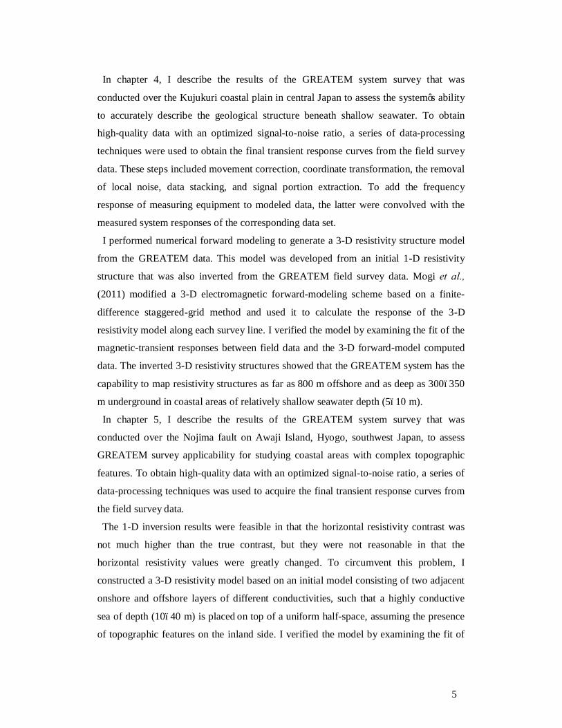
In chapter 4, I describe the results of the GREATEM system survey that was

conducted over the Kujukuri coastal plain in central Japan to assess the system’s ability

to accurately describe the geological structure beneath shallow seawater. To obtain

high-quality data with an optimized signal-to-noise ratio, a series of data-processing

techniques were used to obtain the final transient response curves from the field survey

data. These steps included movement correction, coordinate transformation, the removal

of local noise, data stacking, and signal portion extraction. To add the frequency

response of measuring equipment to modeled data, the latter were convolved with the

measured system responses of the corresponding data set.

I performed numerical forward modeling to generate a 3-D resistivity structure model

from the GREATEM data. This model was developed from an initial 1-D resistivity

structure that was also inverted from the GREATEM field survey data. Mogi et al.,

(2011) modified a 3-D electromagnetic forward-modeling scheme based on a finite-

difference staggered-grid method and used it to calculate the response of the 3-D

resistivity model along each survey line. I verified the model by examining the fit of the

magnetic-transient responses between field data and the 3-D forward-model computed

data. The inverted 3-D resistivity structures showed that the GREATEM system has the

capability to map resistivity structures as far as 800 m offshore and as deep as 300–350

m underground in coastal areas of relatively shallow seawater depth (5–10 m).

In chapter 5, I describe the results of the GREATEM system survey that was

conducted over the Nojima fault on Awaji Island, Hyogo, southwest Japan, to assess

GREATEM survey applicability for studying coastal areas with complex topographic

features. To obtain high-quality data with an optimized signal-to-noise ratio, a series of

data-processing techniques was used to acquire the final transient response curves from

the field survey data.

The 1-D inversion results were feasible in that the horizontal resistivity contrast was

not much higher than the true contrast, but they were not reasonable in that the

horizontal resistivity values were greatly changed. To circumvent this problem, I

constructed a 3-D resistivity model based on an initial model consisting of two adjacent

onshore and offshore layers of different conductivities, such that a highly conductive

sea of depth (10–40 m) is placed on top of a uniform half-space, assuming the presence

of topographic features on the inland side. I verified the model by examining the fit of

6

the magnetic-transient responses between field data and the 3-D forward-model

computed data. The inverted 3-D resistivity structures showed that the GREATEM

system has the capability to map underground resistivity structures as deep as 500 m

onshore and offshore. The GREATEM survey delineated how seawater intrudes on the

landside of the fault.

In chapter 6, I provide a general summary of the whole thesis and propose future

research.

7

Chapter 2

GREATEM System's Fundamentals and Specifications

2.1. The GREATEM System

The GREATEM system was described in details by Mogi et al., (2009) and Okazaki et

al., (2011), here I describe based on their description. The GREATEM uses a grounded

electrical dipole source of 2-3 km length as a transmitter and a three-component

magnetometer in the towed bird as a detector (Figure 2.1). With a grounded source, a

large-moment source can be applied and a long transmitter-receiver distance used,

yielding a greater depth of investigation but limiting the survey area. Other advantages

include a smaller effect of flight altitude and the possibility of higher-altitude

measurements.

Data are recorded in the time domain, providing raw time series of the magnetic fields

induced by eddy currents in the ground after cutting off the transmitting current,

meaning that a noise filter can be easily introduced. The GREATEM system is

considered to be an airborne version of the Long Offset Transient Electromagnetics

(LOTEM) system (Strack, 1992), one of the electromagnetic survey systems used in

surveying deeper structures. Transient data acquisition in the time domain after cutting

off the source current has advantages for deeper exploration because it avoids the near-

field effect (Goldstein and Strangway, 1975) that is included in frequency-domain data.

Mogi et al. (1998) described the early stages of GREATEM system development and

gave the system its acronym. In addition, they illustrated some theoretical transient

responses of magnetic fields in the air for horizontally layered structures and noted

several features of the GREATEM response, such as depth of investigation, effect of

measuring height, and source-receiver distance. They also highlighted the system’s

advantages in investigating deeper structures and the possibility of identifying resistivity

8

structure responses from heights of 100-200 m. This is important for improving the

safety of AEM surveys.

Although time-domain data stacking on a moving aircraft is limited, important

technical problems must be overcome, such as monitoring and filtering motion noise in

the data, cancelling natural magnetic field variation, and limiting cultural noise. A high-

accuracy fiber-optic gyro (Japan Aviation Electronics Industry, JCS7401) to monitor the

motion of the bird, and a magneto-impedance (MI) sensor (Mohri et al., 2002) to

monitor direction were both set on gimbals, and a three component induction-coil

magnetometer was installed at the rear of the gimbal mount. These instruments and the

batteries were placed in the bird, and the data-acquisition instruments, consisting of a

data-control PC and a high-precision clock synchronized with the transmitter-control

clock, were set up in the helicopter cabin. Recently, the data-acquisition equipment

installed in the small container and it towed at 10m above the bird. Full time-series data

were collected to facilitate the elimination of noise. The three-component time

derivative of magnetic fields, motions detected by the roll, pitch, and three-axis

acceleration systems, and direction and position were digitized at the rate of 80μsec

using a 16-bit analog to digital (A/D) converter. An identical three-component coil on

the ground monitored natural and cultural noise in the survey area.

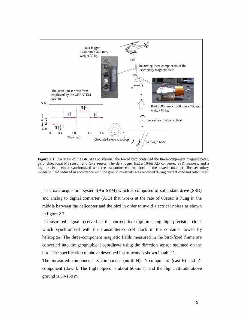
2.2. Measuring Equipment Specifications Figure 2.2, a schematic diagram showing the GREATEM Airborne EM. Transmitted

current is interrupted using high-precision clock which is synchronized with the control

clock in the data acquisition system. Transmitted waveform is +, 0, -, 0 form and each

time interval is 0.4 sec in standard manner as shown in figure 2.1.

In order to decrease the contact resistance across the ground, the cable is trailed and

snaked on both transmission source sides, and about 300 ground electrodes is installed

in the ground in each side, so in two sides was installed about 600 steel bar electrodes.

The current power to the ground is expected to be 20 - 30 A.

Received data are converted to digital form using an A/D converter with resolution of

the 16 bit and a sampling rate at 80μsec. A 0.8 second half cycle of 10,000 pieces of

data are obtained. The files are saved as a 1-cycle of 1.6 seconds. The receiving devices

are mounted in the bird and towed from a helicopter with 40m long rope.

9

The data-acquisition system (Air SEM) which is composed of solid state drive (SSD)

and analog to digital converter (A/D) that works at the rate of 80μsec is hung in the

middle between the helicopter and the bird in order to avoid electrical noises as shown

in figure 2.3.

Transmitted signal received at the current interruption using high-precision clock

which synchronized with the transmitter-control clock in the container towed by

helicopter. The three-component magnetic fields measured in the bird-fixed frame are

converted into the geographical coordinate using the direction sensor mounted on the

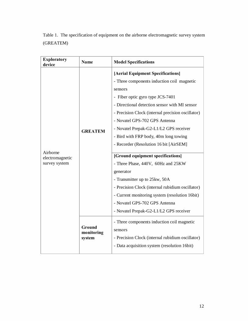
bird. The specification of above described instruments is shown in table 1.

The measured components X-component (north-N), Y-component (east-E) and Z-

component (down). The flight Speed is about 50km/ h, and the flight attitude above

ground is 50-150 m.

Data logger 1230 mm x 320 mm, weight 30 kg

Geologic body Grounded electric source

Recording three components of the secondary magnetic field

Bird 2000 mm x 1000 mm x 700 mm, weight 80 kg

Secondary magnetic field

The actual pulse waveform employed by the GREATEM system

Time (sec) 0 0.4 0.8 1.2 1.6

-5000

5000

Am

plitu

de

(

mV

)

Figure 2.1. Overview of the GREATEM system. The towed bird contained the three-component magnetometer, gyro, directional MI sensor, and GPS sensor. The data logger had a 16-bit AD converter, SSD memory, and a high-precision clock synchronized with the transmitter-control clock in the towed container. The secondary magnetic field induced in accordance with the ground resistivity was recorded during current ‘on’ and ‘off’ times.

10

Figure 2.2. Schematic diagram showing the GREATEM Airborne EM

Electrodes

Cable

Bird

Receiver

Transmitter

Dipole antenna

11

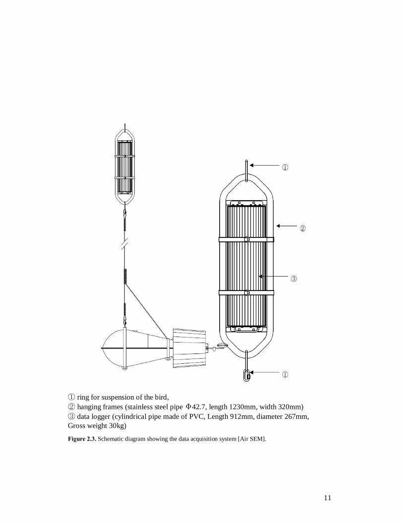
① ring for suspension of the bird, ② hanging frames (stainless steel pipe Φ42.7, length 1230mm, width 320mm) ③ data logger (cylindrical pipe made of PVC, Length 912mm, diameter 267mm, Gross weight 30kg) Figure 2.3. Schematic diagram showing the data acquisition system [Air SEM].

12

Table 1. The specification of equipment on the airborne electromagnetic survey system

(GREATEM)

Exploratory device Name Model Specifications

[Aerial Equipment Specifications]

- Three components induction coil magnetic

sensors

- Fiber optic gyro type JCS-7401

- Directional detection sensor with MI sensor

- Precision Clock (internal precision oscillator)

- Novatel GPS-702 GPS Antenna

- Novatel Prepak-G2-L1/L2 GPS receiver

- Bird with FRP body, 40m long towing

- Recorder (Resolution 16 bit [AirSEM]

GREATEM

[Ground equipment specifications]

- Three Phase, 440V, 60Hz and 25KW

generator

- Transmitter up to 25kw, 50A

- Precision Clock (internal rubidium oscillator)

- Current monitoring system (resolution 16bit)

- Novatel GPS-702 GPS Antenna

- Novatel Prepak-G2-L1/L2 GPS receiver

Airborne electromagnetic survey system

Ground monitoring system

- Three components induction coil magnetic

sensors

- Precision Clock (internal rubidium oscillator)

- Data acquisition system (resolution 16bit)

13

2.3. Data Processing In the following section, I describe the advanced data-processing techniques performed

to obtain a final transient response curve.

2.3.1. Movement Correction

Movement correction was performed using a transfer function relating variations in the

recorded magnetic field to magnetometer movement, as monitored by the gyro. We used

a highly accurate gyro to correct for the movement of the sensor. This correction was

confirmed in previous surveys by Mogi et al. (2009) and Okazaki et al. (2011). The

transfer function was calibrated at a time when no signal was applied. Corrections were

made by subtracting predicted magnetic field variations using the transfer function

based on the movement measured by the gyro from the observed magnetic field

variations to yield data that were free from motion noise. Figure 2.4(A) shows an

example of a raw waveform of received signal, and figure 2.4(B) shows an example of

magnetic field data before (green lines) and after (red lines) the movement correction.

Small transient responses remain but are clearly distinguishable in the motion-corrected

time-series. The magnetic field data after movement correction at an increased

resolution are shown in figure 2.4(C).

2.3.2. Coordinate Transformation

The transformation of magnetic field components from bird-based coordinates to

geographical coordinates was based on the directional sensor data. The coordinate

transformation correction was made using a tri-axis orthogonal coordinate

transformation.

2.3.3. Removal of Local Noise

Magnetic field data obtained from the ground magnetometer were used to remove

natural and artificial noise, as necessary. Multiple stacking provided the precise

waveform induced by the transmitted signal at the ground-monitor site. The signature of

local noise was incoherent because of the transmitter signal (TX) and airborne system

movement. The noise involved in each set of time-series data was obtained by

14

subtracting the signal from each set of the monitored data, which was then subtracted

from a set of concurrent airborne data.

When necessary, data stacking was used to minimize random noise. Because the

helicopter was moving at 50 km/h, or 14 m/sec, the sensor moved about 22 m during

one 1.6-sec cycle. A transient signal was present after the current cut-off twice in each

cycle, so that one transient response could be inferred for each 11 m of survey distance.

After stacking n times, the stacked data covered 11 n meters. Three to six transient

signals were summed to reduce the noise waveform. Examples of signals after the 12th

and 24th stackings are shown in figures 2.4(D) and 2.4(E), respectively.

2.4. Inversion for Assumed Layer Structure 2.4.1. Correction of Instrument Frequency Response

The received signals contain both of transmitted signals by the source and reflected

ones by underground structure also the frequency characteristics of instruments.

Considering the characteristics curve analysis of the instruments (Figure 2.5), if, the

received signal (Y) at the instrument frequency response (G), and the subsurface

response wave (X) in time domain, so

where t is time and x is convolution multiples.

Therefore, after the transformation to the frequency domain, the frequency response of

the subsurface response given by the following formula

( )( )( )

Y wX wG w

= (2.2)

where ω is the angular frequency. Finally, using inverse Fourier transform for X (ω), the

time-domain wave x (t) can be obtained. The obtained waveform x (t) will be consistent

with the resistivity structure.

This is normal method to remove system response of equipment from field data. But,

deconvolution in Eq. (2.2) is unstable and affected much by noise. It is better to use a

method that convoluted theoretical response with system response to subsurface

response wave. Eq. (2.1) is using to structural analysis compared with field responses

including system response.

( ) ( ) ( )XY t X t G t= (2.1)

15

Time (sec)

Rel

ativ

e in

tens

ity b

y

max

imum

am

plitu

de (m

V)

(C)

Time (sec)

Rel

ativ

e in

tens

ity b

y

max

imum

am

plitu

de (m

V)

(B)

(A) 1.2 0.4 0.8 1.60

Time (sec)

Time (msec)

Signal

(E)

Rel

ativ

e in

tens

ity b

y

max

imum

am

plitu

de (m

V)

Signal

(D) Time (msec)

Rel

ativ

e in

tens

ity b

y

m

axim

um a

mpl

itude

(mV

)

Waveform

Movement correction

Data Stacking

Con

vert

to o

rthog

onal

di

rect

ions

Time (msec)

Signal

Zero level

(F)

Rel

ativ

e in

tens

ity b

y

max

imum

am

plitu

de (m

V)

Figure 2.4. Flow chart of the data processing: (A) example of a raw waveform, (B) three-component time-domain magnetic field data. Lines denote the data before (green) and after (red) motion correction. (C) enlarged resolution of the magnetic fields after motion correction, (D) Signal after 12th stacking, (E) Signal after 24th stacking and (F) an example of a final noise-free signal after determination of zero level.

Decide zero level

16

2.4.2. Theoretical Analysis

Usually, vertical component of the magnetic field (Hz) in frequency domain is used in

analyzing subsurface structure, assuming the horizontally layered earth because

responses are simpler and effect of natural noise is smaller than horizontal components.

Using the basic theory of the transmission sources (small dipole source) in case of

horizontal layered, (Ward and Hohmann, 1988; Spies and Frischknecht, 1991), the

magnetic field is:

2 22 4 [3 (3 3 ) ]

2P ikrHz ikr k r eлk r

− −= − + − (2.3)

where P is electrical dipole moment, r is the transmitter-receiver separation and k is

propagation constant or wave number for lower half space and given by

1/2( )k iσµω= − (2.4)

where σ is the conductivity, µ the magnetic permeability and ω is the angular

frequency. The ssolution is obtained in the frequency domain and it is necessary to

convert from time-domain data using the inverse Fourier transformation.

After the previous data processing and corrections were made, the noise-free transient

response x(t) as shown in figure 2.4(F) was inverted to determine a 1-D resistivity

structure. I used the part of the transient response with less dispersion due to noise and

Amplitude

Figure Figure 2.5. Comparison of the frequency characteristic of instruments when the power is switched on (under primary field) / switched off (no primary field)

Phase

Pow

er (d

B)

17

Time (sec)

Transit field data Transit curve Calculated layered model)

Rel

ativ

e in

tens

ity b

y

max

imum

am

plitu

de (d

hz/d

t)

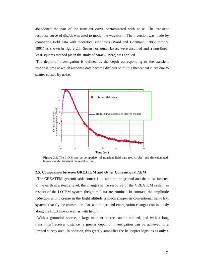
Figure 2.6. The 1-D inversion comparison of transient field data (red circles) and the calculated, layered-model transient curve (blue line).

abandoned the part of the transient curve contaminated with noise. The transient

response curve of dhz/dt was used to model the waveform. The inversion was made by

comparing field data with theoretical responses (Ward and Hohmann, 1988; Jomori,

1991) as shown in figure 2.6. Seven horizontal layers were assumed and a non-linear

least-squares method (as in the study of Strack, 1992) was applied.

The depth of investigation is defined as the depth corresponding to the transient

response time at which response data become difficult to fit to a theoretical curve due to

scatter caused by noise.

2.5. Comparison between GREATEM and Other Conventional AEM

The GREATEM system’ cable source is located on the ground and the pulse injected

to the earth at a steady level, the changes in the response of the GREATEM system in

respect of the LOTEM system (height = 0 m) are nominal. In contrast, the amplitude

reduction with increase in the flight altitude is much sharper in conventional heli-TEM

systems that fly the transmitter also, and the ground energization changes continuously

along the flight line as well as with height.

With a grounded source, a large-moment source can be applied, and with a long

transmitter–receiver distance, a greater depth of investigation can be achieved in a

limited survey area. In addition, this greatly simplifies the helicopter logistics as only a

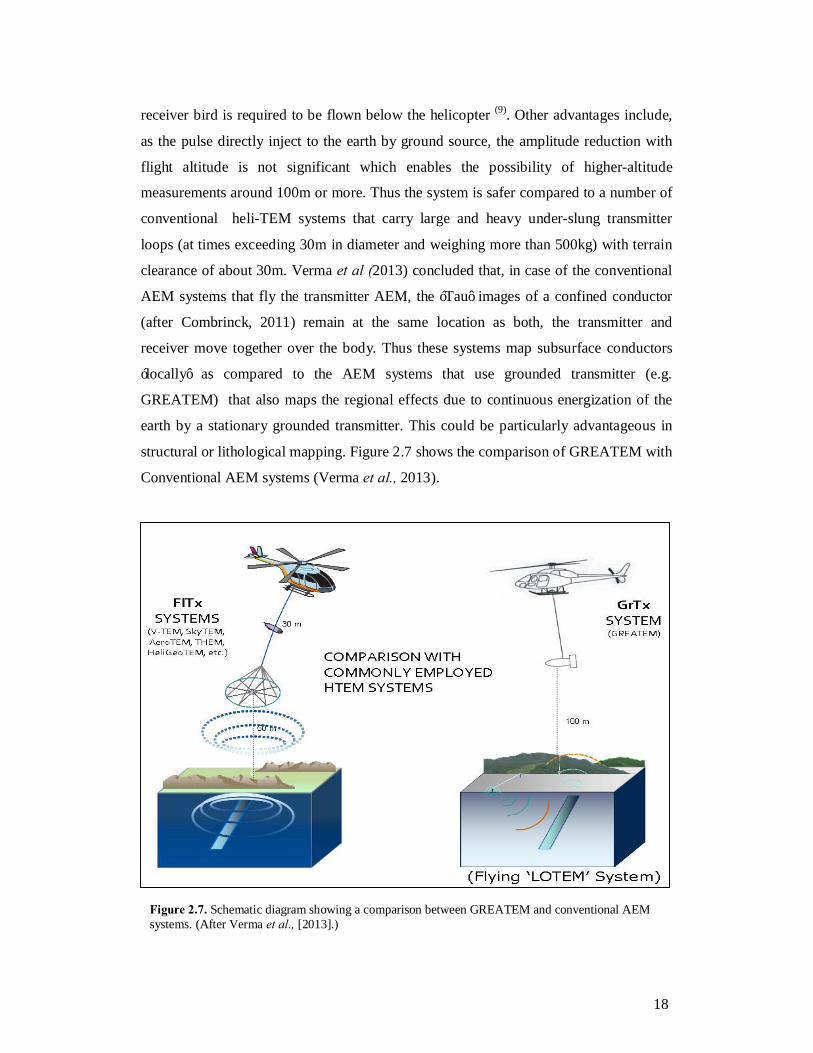
18

receiver bird is required to be flown below the helicopter (9). Other advantages include,

as the pulse directly inject to the earth by ground source, the amplitude reduction with

flight altitude is not significant which enables the possibility of higher-altitude

measurements around 100m or more. Thus the system is safer compared to a number of

conventional heli-TEM systems that carry large and heavy under-slung transmitter

loops (at times exceeding 30m in diameter and weighing more than 500kg) with terrain

clearance of about 30m. Verma et al (2013) concluded that, in case of the conventional

AEM systems that fly the transmitter AEM, the ‘Tau’ images of a confined conductor

(after Combrinck, 2011) remain at the same location as both, the transmitter and

receiver move together over the body. Thus these systems map subsurface conductors

‘locally’ as compared to the AEM systems that use grounded transmitter (e.g.

GREATEM) that also maps the regional effects due to continuous energization of the

earth by a stationary grounded transmitter. This could be particularly advantageous in

structural or lithological mapping. Figure 2.7 shows the comparison of GREATEM with

Conventional AEM systems (Verma et al., 2013).

Figure 2.7. Schematic diagram showing a comparison between GREATEM and conventional AEM systems. (After Verma et al., [2013].)

19

Chapter 3

Three-dimensional Electromagnetic Modeling of Sea and Topographic Effects

on GREATEM Survey Data 3.1. Introduction A resistivity structure with a horizontally layered structure might be distorted in the

case of large resistivity contrasts, such as between land and sea in coastal areas and

between the air and topographic features considered as anomalies in the air layer. To

overcome these issues, I used the 3-D EM numerical modeling utilizing a SFD method

developed by Fomenko and Mogi (2002) to study the effects of both sea and topography

on GREATEM survey data.

3.2. Three-dimension Forward Modeling Theory

The 3-D EM forward algorithm used in this study draws on the SFD method

developed by Fomenko and Mogi (2002), which involves the special pre-whitening of a

large matrix to the improve the stability of computation and a devised solver. It is

designed for computer calculation of the electrical (E) and magnetic (H) field

components resulting from secondary EM fields, which are induced by the primary EM

field in 3-D anomalies on a horizontal multi-layer structure. This approach is used to

improve the accuracy of models with a high resistivity contrast over a wider frequency

range. To apply it to a GREATEM study, we modified this algorithm by adding a

source term of a grounded electrical-dipole source (Mogi et al., 2011). To compute a

finite-length electrical-dipole source term, we used the formulae for a long grounded

wire on a layered Earth described by Ward and Hohmann (1988), equations 4.184–

4.190 in their book.

Here, I describe the formulation of the SFD method after Fomenko and Mogi (2002).

The time-domain EM responses were computed by sine or cosine transformation from

the frequency-domain data. The range of computing in the frequency domain is 105 to

20

10-2 Hz and transient time responses were obtained at 10-4 to 100 s. In forward modeling,

the second-order partial differential equations for scalar and vector potential are

discretized on a SFD method (after Fomenko and Mogi, 2002; Mogi et al., 2011).

Figure 3.1 shows the staggered grid cell used for this algorithm computation.

Assuming the time harmonic dependence e–iwt (w: angular frequency) and ignoring the

displacement current in magnetotelluric modeling, Maxwell’s equations for the total

electric (E) and magnetic field (H) in a staggered grid lead to

' 'HdI Edsσ=∫ ∫∫Ñ (3.1) EdI i Hdsωµ=∫ ∫∫Ñ (3.2) ( )

ijkdVE ds oσ =∫Ñ , or ( ) 0div Eσ= = (3.3)

( )

jkdViH ds o=∫Ñ , or 0divH = (3.4)

where µ is the magnetic permeability and σ is the conductivity destitution the cells of a normal grid, ds correspond to the normal grid cells and 'ds correspond to the central grid cells.

After SFD approximation of Eqs. (3.1) - (3.4) we obtain six scalar equations shown as

(3.5 -3.10)

' '

1/ 2 1/2 1 1/ 2 1/2 1

' ', 1, 1 1/2, , 1 1

( ) ( )

( )

z z y yj j k k k j

x xi j k i j k j k

H H H H

Eσ+ − − + − −

− − − − −

− ∆ − − ∆

= ∆ ∆ (3.5)

Figure 3.1. A staggered grid cell V (i, j, and k). Tangential electric and normal magnetic field components are sampled at the center of edges (E) and at the center of interfaces (H), all of them continuous. Δi, Δj, and Δk denote the sizes of the cells (after Fomenko and Mogi, 2002).

21

' '

1/2 1/2 1 1/2 1/2 1' '

1, , 1 , 1/ 2, 1 1

( ) ( )( )

x x z zk k i i i k

y yi j k i j k k i

H H H HEσ

+ − − + − −

− − − − −

− ∆ − − ∆

= ∆ ∆ (3.6)

' '

1/2 1/2 1 1/2 1/2 1

' ', 1, , , 1/2 1 1

( ) ( )

( )

y y x xi i j j j i

y zi j k i j k i j

H H H H

Eσ+ − − + − −

− − − −

− ∆ − − ∆

= ∆ ∆ (3.7)

' '

1 1 1 1

, 1/ 2, 1/2 1 1

( ) ( )z z y yj j k k k j

xi j k j k

E E E E

i Hωµ− − − −

− − − −

− ∆ − − ∆

= ∆ ∆ (3.8)

' '

1 1 1 1

1/ 2, , 1/2 1 1

( ) ( )x x z zk k i i i k

yi j k k i

E E E Ei Hωµ

− − − −

− − − −

− ∆ + − ∆

= ∆ ∆ (3.9)

' '

1 1 1 1

1/ 2, 1/ 2, 1 1

( ) ( )y x x zi i j j j i

zi j k i j

E E E E

i Hωµ− − − −

− − − −

− ∆ + − ∆

= ∆ ∆ (3.10)

where for example,

1, 1, , , 1, , 1

, 1, 1

' '1, 1, 1 1 1 1

( ) [

] / (4 )

zi j k i j k i j i j k i j

i j k i j

i j k i j i j

σ σ σ

σ

σ

− − − −

− −

− − − − − −

= ∆ ∆ + ∆ ∆

+ ∆ ∆

+ ∆ ∆ ∆ ∆

(3.11)

The H field is calculated using the curl-operator in Eqs. (3.8-3.10). Tangential electric

and normal magnetic field components are continuous at the staggered grid due to the

selection of grid nodes. It helps to stably calculate the magnetic Hz component in the

center of cell interfaces Xi +1/2, Yj+1/2 at each level Z = Zk by using equation (3.10).

The original system describing Eqs. (3.5-3.10) is a pair of coupled first-order equations

for E and H. In order to decrease the number of equations, H-field eliminated from Eqs.

(3.5-3.7) using the right-hand side of Eqs. (3.8-3.10), the second-order SFD equation

was introduced as follows:

~ ~( ) 0s p totalA E E AE+ = = (3.12)

The matrix~A is neither Hermitian nor symmetric, but it can be transformed to the

complex symmetric matrix ^A by multiplying the obtained equations by factor i∆ for Ex

members in the right side, j∆ for Ey and k∆ for Ez.

22

3.3. Verification of the Forward Computing Algorithm

I have verified our 3-D electromagnetic (EM) modeling-computing scheme described

previously. Verification is based on the 3-D modeling method by comparing the results

of a quarter-space and trapezoidal hill models with the results of the 2.5-D finite-

element method (FEM) by Mitsuhata (2000), and the 3-D finite-difference program with

the spectral Lanczos decomposition method (SLDM) developed by Druskin and

Knizhnerman (1994), which was described in Mitsuhata (2000). The models used to

perform this verification were similar to that described by Mitsuhata (2000).

3.3.1. Quarter-space Model

The quarter-space model shown in Figure 3.2 consists of two quarter-spaces. On the

left of the contact, the resistivity is 1 Ω-m, and on the right, 10 Ω-m. A horizontal

electrical dipole (HED) source is directed to the y-axis and is situated on the surface at

x=˗2250 m to the left of the contact.

Figure 3.3 shows the result in the time domain from 0.01 to 10 s at the sites near the

contact. To check the validity of my computation method, the results of the time

derivative of the vertical magnetic fields (Hz) obtained from 3-D SFD are compared

with both of the results obtained by the 2.5-D FEM by Mitsuhata (2000) and the 3-D

SLDM developed by Druskin and Knizhnerman (1994). Although minor differences

exist, the main features of the three results are similar. At x= ˗750 m, the results are

nearly equal to the analytical solutions for the homogeneous half-space of 1 Ω-m.

Figure 3.2. A quarter-space model. The Earth is divided by a vertical fault at x = 0 m. A y-directed horizontal electrical dipole (HED) source is situated on the left side of the contact. Four receiver sites are situated around the contact. (Modified from Mitsuhata [2000].)

23

However, early time depressions begin to appear at x = ˗250 m. On the right side of the

contact at x = 250 m, the depression becomes too strong and turns to a sign reversal. At

x = 750 m, it becomes somewhat weak and the reversal disappears.

(B)

(C) (D)

(A)

Figure.3.3. (A), (B), (C), and (D) are comparisons of the time derivatives of vertical magnetic fields (hz) obtained from the 3-D SFD, FEM 2.5-D, and SLDM 3-D modeling code for the quarter-space model (Figure 3.2) at the four measuring points (x = ˗750, ˗250, 250, and 750 m). The analytical solutions for a homogeneous half-space of 1 Ω-m are shown together. The (+) and (˗) signs indicate the response. (Modified from Mitsuhata [2000].)

24

3.3.2. Trapezoidal Hill with a Conductive Block Model This model consists of a trapezoidal hill over a uniform 100 Ω-m half-space with an

embedded conductive block of 1 Ω-m. A y-directed HED source is located on the Earth

surface x = 0 m. The center of the hill is at x = 2000 m. The conductive block is situated

between the source and the hill. Two receiver sites are on the hill at x = 2000 m and on

the right side at x = 6500 m, as shown in Figure 3.4. The 3-D SFD used a rectangular

grid, and a slope was modeled by tiers of grids.

Figure 3.5 shows comparisons of the time derivatives of hz response among the results

obtained by 3-D SFD, those by 2.5-D FEM (Mitsuhata, 2000), and the response of a flat

homogeneous half-space of 100 Ω-m for reference. Although minor differences occur,

the main features of these results are similar.

At both sites, the differences in the responses for the topographic model and

homogeneous half-space are small. In contrast, the influence of the conductive block is

significant. These results have verified the accuracy of our 3-D SFD computation

algorithm and its viability for modeling complex structures and admitting interpretations

Figure.3.4. A trapezoidal hill with a conductive block of 1 Ω-m. A y-directed HED source is located on the Earth surface at x = 0 m. The center of the hill is at x = 2000 m. The conductive block is situated between the source and the hill. Two receiver sites are on the hill and on the right side. (Modified from Mitsuhata [2000].)

25

considering both topography and inhomogeneities located near the source and between

the source and the receiver.

3.4. Model Descriptions and Results 3.4.1. Sea-land Boundary Model As shown in Figure 3.6, the sea–land boundary model consisted of two adjacent layers

of different conductivity, in which the sea was a thin-sheet conductor (0.3 Ω-m) placed

on the top of a uniform half-space Earth medium (100 Ω-m). The 3-D modeling area

was x: (˗20 km, 15 km), y: (˗20 km, 20.4 km), and z: (˗12.2 km, 12 km). The model was

composed of 40 × 29 × 28 = 32,480 cells.

The node spacing was small near the source (50 m) and gradually coarsened with

increasing distance from the source in a horizontal direction. In the vertical direction,

the size of each grid varied from 5 m at the surface to 3200 m at the top and bottom of

the model, as shown in Figure 3.7.

The EM responses were calculated for different positions of the grounded electrical

source (at 10, 20, and 300 m) from the shoreline landward, and the uniform half-space

Figure 3.5. Comparisons of the time derivatives of hz obtained from 3-D SFD and FEM 2.5-D modeling code for the trapezoidal hill model of Figure 3.4 with/without a conductive block. The analytical solutions for a homogeneous half-space of 100 Ω-m are shown together. (Modified from Mitsuhata [2000].)

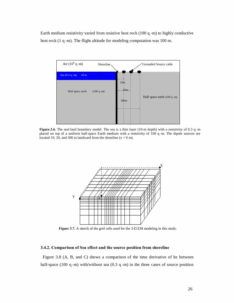
26

Earth medium resistivity varied from resistive host rock (100 Ω-m) to highly conductive

host rock (1 Ω-m). The flight altitude for modeling computation was 100 m.

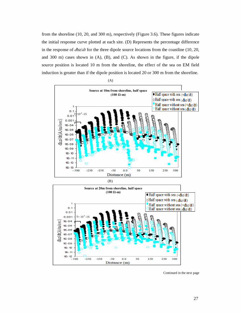
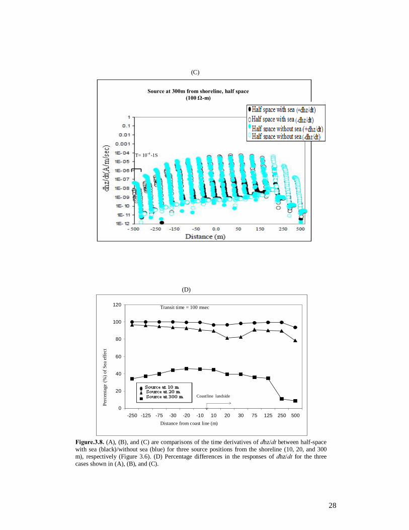
3.4.2. Comparison of Sea effect and the source position from shoreline

Figure 3.8 (A, B, and C) shows a comparison of the time derivative of hz between

half-space (100 Ω-m) with/without sea (0.3 Ω-m) in the three cases of source position

Figure.3.6. The sea–land boundary model. The sea is a thin layer (10-m depth) with a resistivity of 0.3 Ω-m placed on top of a uniform half-space Earth medium with a resistivity of 100 Ω-m. The dipole sources are located 10, 20, and 300 m landward from the shoreline (x = 0 m).

Shoreline Grounded Source cable

10m

20m

Half space earth (100 Ω-m) 300m

Half space earth (100 Ω-m)

Sea (0.3 Ω-m) 10 m

Air (108 Ω-m)

Z Y

X

Figure 3.7. A sketch of the grid cells used for the 3-D EM modeling in this study.

27

from the shoreline (10, 20, and 300 m), respectively (Figure 3.6). These figures indicate

the initial response curve plotted at each site. (D) Represents the percentage difference

in the response of dhz/dt for the three dipole source locations from the coastline (10, 20,

and 300 m) cases shown in (A), (B), and (C). As shown in the figure, if the dipole

source position is located 10 m from the shoreline, the effect of the sea on EM field

induction is greater than if the dipole position is located 20 or 300 m from the shoreline.

Continued in the next page

(A)

T=10-4 -1S

Source at 10m from shoreline, half space (100 Ω-m)

(B)

Source at 20m from shoreline, half space (100 Ω-m)

T= 10-4 -1S

28

0

20

40

60

80

100

120

-250 -125 -75 -30 -20 -10 10 20 30 75 125 250 500

Transit time = 100 msec

Per

cent

age

(%) o

f Sea

eff

ect

Coastline landside

Distance from coast line (m)

(D)

Figure.3.8. (A), (B), and (C) are comparisons of the time derivatives of dhz/dt between half-space with sea (black)/without sea (blue) for three source positions from the shoreline (10, 20, and 300 m), respectively (Figure 3.6). (D) Percentage differences in the responses of dhz/dt for the three cases shown in (A), (B), and (C).

(C)

T= 10-4 -1S

Source at 300m from shoreline, half space (100 Ω-m)

29

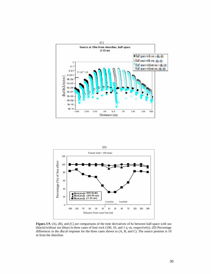
3.4.4. Comparison of Sea Effect and Host Rock Resistivity

To study the relationship between the sea effect and host rock conductivity, I repeated

the computation of the sea–land boundary model (Figure 3.6) with uniform half-space

Earth medium resistivities of 10 and 1 Ω-m, instead of 100 Ω-m. Figure 3.9 (A, B, and

C) shows the comparison of time derivative of hz between half-space with/without sea

in the three cases of half-space resistivities (100, 10, and 1 Ω-m)) respectively. The

source is located at 10 m from the shoreline.

Continued in the next page

(A)

Source at 10m from shoreline, half space (100 Ω-m)

T= 10-4 -1S

(B)

Source at 10m from shoreline, half space (10 Ω-m)

T=10-4 -1S

30

Source at 10m from shoreline, half space (1 Ω-m)

T=10-4 -1S

(C)

(D)

0

20

40

60

80

100

120

-250 -125 -75 -30 -20 -10 10 20 30 75 125 250 500

Distance from coast line (m)

P

erce

ntag

e (%

) of S

ea e

ffec

t

Transit time= 100 msec

Landside Coastline

Figure.3.9. (A), (B), and (C) are comparisons of the time derivatives of hz between half-space with sea (black)/without sea (blue) in three cases of host rock (100, 10, and 1 Ω-m, respectively). (D) Percentage differences in the dhz/dt response for the three cases shown in (A, B, and C). The source position is 10 m from the shoreline.

31

(D) An example of the sea effect represented by the percentage difference in the

response of dhz/dt for the three cases showed in (A), (B), and (C). The effect of the sea

on EM field induction is greater for a host rock resistivity of 100 Ω-m than for host rock

conductivities of 10 and 1 Ω-m.

This indicates that the effect of the sea on EM induction is inversely proportional to

the host rock conductivity.

3.4.5. Topography Model

Topography in our model was represented as an anomaly in the air layer in which

resistivity was assumed at 108 Ω-m. I selected a 3-D topographic model consisting of a

topographic feature (100 Ω-m) placed on top of a uniform half-space Earth medium

(100 Ω-m) as shown in figure 3.10.

The resistivity contrast was 106 times between the air and the topography. In the

topographic area, I used x: 50 × y: 50 × z: 25-m cells. Outside the topographic area,

irregular cells were used. The total number of nodes was 52 × 38 × 32 = 63,232 cells.

The computations were performed for four topographic slope angles (α) = 90°

(topography width is 200 m [x = 0–200 m], and its height is 200 m), (α) = 45°

[topography width is 200 m (x = 0–200 m), and its height is 200 m], (α) = 26°

[topography width is 400 m (x = 0–400 m), and its height is 200 m] and (α) = 14°

Figure 3.10. The 3-D topography models. Topography (100 Ω-m) with different slope angles (α) placed on top of a uniform half-space Earth medium (100 Ω-m).

32

[topography width is 800 m (x = 0–800 m), and its height is 200 m]. In the four cases,

the topography width in the y direction is 4000 m (y = ˗2000 to 2000 m), as shown in

figure 3.10. A horizontal electrical dipole source was directed along the y-axis situated

at x = ˗1500.

Figure 3.11 shows a comparison of the dhz/dt response for the topographic slope

angles of 14 and 45° with the response of the uniform half-space Earth medium (Figure

3.10) at different ground levels (H). At a low ground level of 50 m, topography has a

significant effect on the EM response, which gradually decreases with increased flight

altitude. Furthermore, a topographic slope angle of 45° showed a greater effect than a

slope angle of 14°.

Figure 3.12 shows the effect of topography represented by the percentage difference in

the response of dhz/dt between the uniform half-space with or without topography for

topographic slope angles 90, 45, 26, and 14° (Figure 3.10) at different ground levels (H).

The effect of topography is most significant for a steep slope angle (90°) than for gentler

Figure 3.11. Comparison of the dhz/dt responses among topography with slope angles (α) of 14° (black), 45° (gray), and a uniform half-space Earth medium (blue) at different ground levels (H). The transient time T =10-4–100 s.

T=10-4 -1S

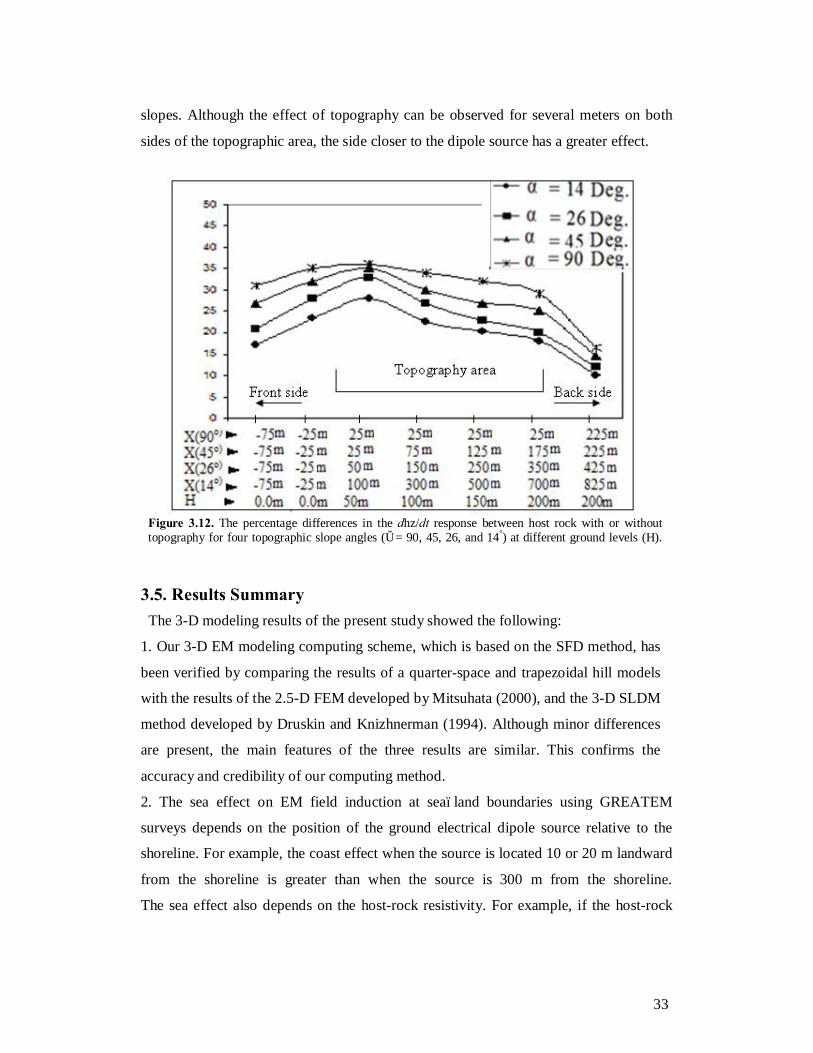
33

slopes. Although the effect of topography can be observed for several meters on both

sides of the topographic area, the side closer to the dipole source has a greater effect.

3.5. Results Summary The 3-D modeling results of the present study showed the following:

1. Our 3-D EM modeling computing scheme, which is based on the SFD method, has

been verified by comparing the results of a quarter-space and trapezoidal hill models

with the results of the 2.5-D FEM developed by Mitsuhata (2000), and the 3-D SLDM

method developed by Druskin and Knizhnerman (1994). Although minor differences

are present, the main features of the three results are similar. This confirms the

accuracy and credibility of our computing method.

2. The sea effect on EM field induction at sea–land boundaries using GREATEM

surveys depends on the position of the ground electrical dipole source relative to the

shoreline. For example, the coast effect when the source is located 10 or 20 m landward

from the shoreline is greater than when the source is 300 m from the shoreline.

The sea effect also depends on the host-rock resistivity. For example, if the host-rock

Figure 3.12. The percentage differences in the dhz/dt response between host rock with or without topography for four topographic slope angles (α = 90, 45, 26, and 14°) at different ground levels (H).

34

resistivity is 100 Ω-m, the effect of the sea on EM field induction is higher than for 10

or 1 Ω-m.

3. The most significant effect of topography on EM field induction occurs at low ground

levels and decreases gradually with increasing ground level. The topographic effect of

steep slope angles (e.g., 90 and 45°) is greater than for gentler slopes (e.g., 26 and 14°).

The percentages of the topography effect are ca. 52, 45, 33, and 29% in the cases of 90,

45, 26, and 14° of topographic slope angle, respectively.

3.6. Conclusions The sea effect on GREATEM survey data is inversely proportional to both the distance

of the dipole source from the shoreline and host-rock conductivity. Topography with

high slope angles has a greater effect than topography with low slope angles. In addition,

the area of the topographic feature closer to the dipole source has a greater effect on EM

field induction for several meters.

The modeling results of this study will be considered when planning future

GREATEM surveys as well as for the reasonable interpretation of data collected in

coastal areas. Although it is encouraging that more studies of the sea effect are

supported by quantitative modeling, the non-uniqueness of EM interpretation is a

persistent problem, and modeling still relies heavily on an obvious presumed structure.

35

Chapter 4

Three-dimensional Resistivity Modeling of a Coastal Area Using GREATEM Survey Data from Kujukuri Beach,

Chiba, Central Japan 4.1. Introduction

Coastal areas are vulnerable to natural disasters such as earthquakes, tsunamis, and

hurricanes (e.g., Mallin and Corbett, 2006; Wang et al., 2006; Hornbach et al., 2010).

Mapping the subsurface physical properties of coastal areas is useful for mitigating

natural disasters and sustaining comfortable environments. An important property is

electrical conductivity, which is increased by the presence of conductive minerals.

Considerable geological heterogeneity in conductivity exists both vertically and

laterally along the coast. Inverted electrical conductivity models provide remarkable

insight into complex coastal stratigraphy and enable a better understanding of

groundwater–surface water exchange processes (Hallier et al., 2008). This information,

together with an appreciation of the significant rising of seawater levels due to tsunamis

and hurricanes, is critical for the sound management of water resources and coastal area

development strategies.

The use of airborne electromagnetic (AEM) techniques for groundwater monitoring

and modeling has increased steadily in the past decade (e.g., Steuer et al., 2009) owing

to advances in AEM systems and processing and in inversion methodologies. However,

few studies have applied AEM in areas such as lagoons, wetlands, rivers, or bays, and

previous studies have mainly focused on bathymetric data (e.g., Vrbancich and Fullagar,

2007). Viezzoli et al. (2010) demonstrated the suitability of the SkyTEM helicopter-

borne transient electromagnetic (EM) system (Sørensen and Auken, 2004) for

investigating surface water and groundwater exchange in transitional coastal

environments. They investigated an area at the southern margin of the Venice Lagoon,

Italy, where very shallow surface water (less than 1 m), tidal marshes, large rivers, and

36

several reclamation channels, combined with a complex morphological, geological, and

hydrological setting, had precluded in-depth traditional investigation. In this coastal area,

AEM data were used to probe the resistivity structure to a depth of ~200 m.

New applications of AEM survey techniques have been introduced in engineering and

environmental fields, particularly for studies involving active volcanoes (Mogi et al.,

2009). Time-domain methods offer advantages over frequency-domain methods, such

as an increased depth of investigation and detail, as well as more accurate mapping of

freshwater/saltwater boundaries (Steuer et al., 2009).

Ships designed for surveying at sea are generally difficult to use in shallow coastal

areas, whereas AEM surveys can span both onshore and offshore areas. Walker et al.

(2004) presented a synthesis of salinity management studies in five South Australian

catchments. The field of airborne geophysics was tailored to answer specific salinity

problems and was then integrated with hydrologic/hydrogeological data and modeling

to contribute to the design and implementation of land-use management strategies.

Wilkinson et al. (2005) integrated airborne geophysical data with more traditional

environmental approaches to map potential salt stores, recharge, and discharge sites in

the Goondoola basin, southwest Queensland, Australia, and subsequently developed

land-management recommendations. In that study, the integration of surficial and

subsurface electromagnetic datasets allowed the researchers to extrapolate and map

surface salinity outbreaks and identify similar landscape settings at risk of developing

salinity from groundwater rise.

One significant problem limiting the use of AEM surveys in lagoons, wetlands, rivers,

and bay areas is the presence of the conductive saline surface water that decreases the

penetration depth of the AEM signal. However, the moment of the transmitter loop has

been increased in recent AEM systems. In other words, their penetration power has

increased, as has the quality of the data obtained. This, together with advances in AEM

modeling and inversion procedures, can produce quantitative results useful for

groundwater modeling in coastal areas.

Real subsurface structures are three-dimensional (3-D) by nature. Although one-

dimensional (1-D) models based on horizontal layers are adequate in many exploration

situations, there are also numerous cases, such as for over thrusts, salt domes, and

anticlines, where 3-D modeling is required (Hoerdt et al., 1992). Here I present a 3-D

37

resistivity modeling study to examine the capability of the GREATEM system (Mogi et

al., 1998) to provide accurate data on coastal areas, especially in the presence of

shallow seawater (Ito et al., 2011). The GREATEM method allows for the application

of a large-moment source and use of a long transmitter–receiver distance, increasing the

survey depth to ~800 m in inland areas (Mogi et al., 2009), compared to the ~300 m

depths possible using conventional AEM techniques.

4.2. Survey Area

Kujukuri Beach is a sandy beach located on the northeast coast of the Boso Peninsula

in Chiba Prefecture, central Japan. It is the second-longest beach in Japan and is located

within 60 km of Tokyo (Figure 4.1). The shore-face is barred, with gradients of 1/150 at

a water depth of 0–5 m and 1/200 at 5–15 m depth (Tamura et al., 2008). The landward

margin of the Kujukuri coastal plain is defined by a plateau and hills, rising to ~30 m

above sea level. Seven rivers run through the strand plain, but their contribution to the

offshore sediment supply off the coast has been relatively small. The landforms on the

Kujukuri plain include beach ridges, sandy dunes, inter-ridge swales, and floodplain

(Moriwaki, 1979). Rows of beach ridges run parallel or sub-parallel to the shoreline.

The subsurface stratigraphy across the central part of the Kujukuri coastal plain has

been revealed from drill core studies conducted by Masuda et al. (2001) and Tamura et

al. (2003). Holocene marine sediments approximately 20 m thick overlie the eroded

Plio-Pleistocene basement rocks and earlier Holocene incised-valley deposits. The

marine sediments consist mostly of very fine to medium sand with mollusc shells and

compose the basal, lower and upper shore-face, and backshore facies, in ascending

order. The base of the marine succession marks the erosional ravinement surface formed

in response to the rapid sea-level rise that occurred during the early and middle

Holocene.

The survey group selected this area for our study because of its shallow seawater depth

and the availability of resistivity data for comparison. Previous studies in the Kujukuri

area were conducted by Mitsuhata et al. (2006), Uehara et al. (2007), and Hayashi et al.

(2009). Mitsuhata et al. (2006) applied three types of ground electromagnetic survey

techniques: audio-frequency magnetotelluric, transient electromagnetic (TEM), and

small loop–loop EM measurements. These studies revealed resistive features to a depth

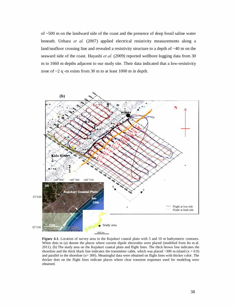
38

of ~500 m on the landward side of the coast and the presence of deep fossil saline water

beneath. Uehara et al. (2007) applied electrical resistivity measurements along a

land/seafloor crossing line and revealed a resistivity structure to a depth of ~40 m on the

seaward side of the coast. Hayashi et al. (2009) reported wellbore logging data from 30

m to 1660 m depths adjacent to our study site. Their data indicated that a low-resistivity

zone of ~2 Ω-m exists from 30 m to at least 1000 m in depth.

Figure 4.1. Location of survey area in the Kujukuri coastal plain with 5 and 10 m bathymetric contours. White dots in (a) denote the places where current dipole electrodes were placed (modified from Ito et.al. 2011). (b) The study area on the Kujukuri coastal plain and flight lines. The thick brown line indicates the shoreline and the thick black line indicates the transmitter cable, which was placed ~300 m inland (x = 0.0) and parallel to the shoreline (x= 300). Meaningful data were obtained on flight lines with thicker color. The thicker dots on the flight lines indicate places where clear transient responses used for modeling were obtained.

Kido River

N

Flight at low tide Flight at high tide

(b)

Y X

140o 450 140o 500 140o 550

35o 630

35o 530 1000 km

5m 10m

Study area

39

4.3. Data Acquisition In the current study, a helicopter-based airborne survey was conducted along 11 flight

lines (line A-line K) spaced 200 m apart (Figure 4.1). Because of flight regulations in

Japan, residential areas were avoided.

The signal source was a time-varying current of ~25 A transmitted underground by a

grounded electrical-dipole source 2.4 km long that was set ~300 m inland parallel with

the shoreline (Figure 4.1). Three components of the secondary magnetic field related to

the underground resistivity were recorded in the atmosphere by a sensor mounted in a

bird towed by the helicopter.

The magnetic field responses were recorded with the current both ‘off’ and ‘on.’ Only

current ‘off’ time data were used because they were of better quality than those for

when the current was ‘on’. The waveforms were digitized through a 16-bit AD

converter at a rate of 80 microseconds (μs), and 20,000 sets of data were recorded

during one cycle of 1.6 seconds (sec). For flight safety, the bird was flown at ~100 m

height, and the measured data were subsequently processed to reduce noise. The sensor

altitude was monitored using a Global Positioning System (GPS) device attached to the

bird, and the sensor height above the ground (terrain clearance) was obtained by taking

the difference between the sensor altitude and the topographic elevation interpolated

from a 50 m grid digital elevation map provided by the Geospatial Information

Authority of Japan.

4.4. Data Processing Options for time-domain data stacking on a moving aircraft are limited. Monitoring

and filtering motion-induced noise in the data, removing natural magnetic field variation,

and limiting cultural noise are important signal conditioning processes that must be

performed. Data processing flow chart used in this study are the same as those described

in figure 2.4 in chapter 2. Finally, after data processing the maximum error of the data

was within 5%.

4.5. One-dimensional Inversion Results

One-dimensional (1-D) results are performed by Ito et al., 2011. Here I describe the

results after them. The waveforms, after noise reduction and stacking, were clear on the

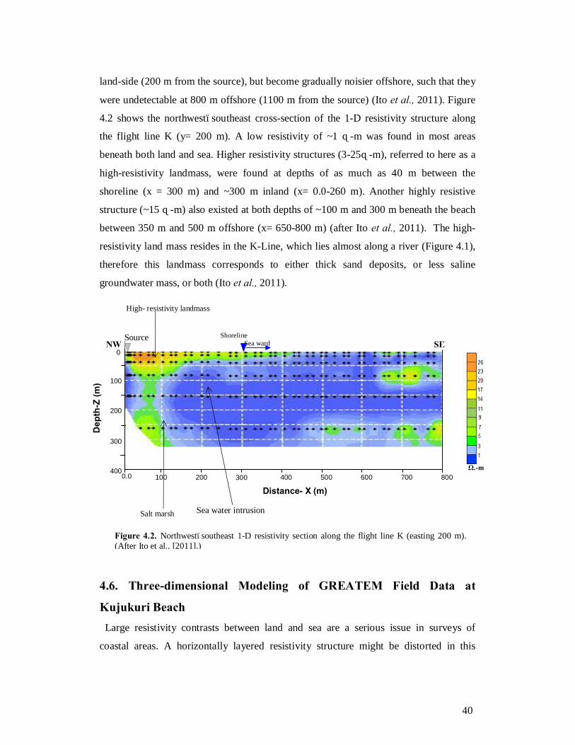
40

land-side (200 m from the source), but become gradually noisier offshore, such that they

were undetectable at 800 m offshore (1100 m from the source) (Ito et al., 2011). Figure

4.2 shows the northwest–southeast cross-section of the 1-D resistivity structure along

the flight line K (y= 200 m). A low resistivity of ~1 Ω-m was found in most areas

beneath both land and sea. Higher resistivity structures (3-25Ω-m), referred to here as a

high-resistivity landmass, were found at depths of as much as 40 m between the

shoreline (x = 300 m) and ~300 m inland (x= 0.0-260 m). Another highly resistive

structure (~15 Ω-m) also existed at both depths of ~100 m and 300 m beneath the beach

between 350 m and 500 m offshore (x= 650-800 m) (after Ito et al., 2011). The high-

resistivity land mass resides in the K-Line, which lies almost along a river (Figure 4.1),

therefore this landmass corresponds to either thick sand deposits, or less saline

groundwater mass, or both (Ito et al., 2011).

4.6. Three-dimensional Modeling of GREATEM Field Data at

Kujukuri Beach Large resistivity contrasts between land and sea are a serious issue in surveys of

coastal areas. A horizontally layered resistivity structure might be distorted in this

Shoreline Sea ward

Dep

th-Z

(m)

Distance- X (m)

NW SE

300

200

100

0

400 100 200 500 600 700 800 300

400

0.0

Source

High- resistivity landmass

Salt marsh

Figure 4.2. Northwest–southeast 1-D resistivity section along the flight line K (easting 200 m). (After Ito et al., [2011].)

Ω.-m

Sea water intrusion

41

situation. Although, the 1-D inversion results of the current study were acceptable in

comparison with previous results by other geophysical methods in the same study area,

they could not reflect the real size and contrast of resistivity features. To overcome this

problem, I tried to construct a 3-D resistivity model that considered large changes in

lateral resistivity. I used the modified SFD method Fomenko and Mogi (2002) and

Mogi et al. (2011) which is described in the chapter 2. To generate the 3-D resistivity

structure model of our study area. A 3-D model of (x: 16.5 x y: 14.2 x z: 9.2) km3 was

designed and divided into (x: 50 x y: 50 x z: 31) = 77500 cells using grid coordinates

similar to the survey area. In the vertical direction, the size of each grid varied from 5 m

at the surface to 6400 m at the top and bottom of the model. The horizontal size was

~200 m in the modeling area, and large-sized (800-6400 m) grids were added at the

circumference of the modeling area to avoid an edge effect. The 3-D resistivity model

was based on an initial model of 1-D resistivity structures inverted from the GREATEM

field survey data. Convolution was applied in the frequency domain to account for the

frequency response characteristics of the field survey instrument. The results were then

compared with the processed survey data of transient response. The field data were

stacked within each cell and the transient response curves of the field data were fitted to

the transient response curve of the 3-D-computed data obtained at the center of the cell.

I used a trial and error method, in that the resistivity values of initial model were

repeatedly changed to obtain a good fit between the 3-D synthetic response and field

data. In the case of the field survey, 10,000 samples of data digitized at a rate of 80 μs

were obtained during half cycle of 0.8 sec. However, in the case of numerical modeling,

40 transient responses were computed at 40 time channels and 10 time-equal spaces of a

log scale in one decade, in the range of 100 μs to 1 sec (4 decades). I therefore used

only those data of the same time channels (30 samples) and computed the root mean-

square error (misfit) between normalized intensity by maximum amplitude (dhz/dt) of

both field data and modeling responses for different blocks of the 3-D model that

corresponded to the survey area. The percent root mean-square misfit was defined as

[|| ∑ (dobs – dcal) ||2/N]1/2 x102.

For all of the 3-D modeling data, the best fit with field data was found with root mean-

square error (RMSE) 2–5%. Examples for different fitting RMSEs of the model

response with field data of the F flight line (RMSE=2%), K flight line (RMSE=3%),

42

and C flight line (RMSE=5%) are shown in figure 4.3 (A, B, and C) respectively. Kinks

and turns appear on the transit response curves owing to the 3-D effects from horizontal

resistivity change. The misfit errors of the 1-D inversion of data on the same flight lines

were about 3.8%, 3.7%, and 5.6%, respectively. In comparison with the 3-D data misfit,

data fitting was improved in the case of the 3-D inversion rather than the 1-D inversion.

The 3-D modeled responses that best fit the field data were used to generate the 3-D

resistivity model of the study area (Figure 4.4).

Time (sec)

A

Nor

mal

ized

inte

nsit

y by

max

am

plitu

de (d

hz/d

t) (A

/m/s

ec)

0.0

0.1

0.2

0.3

0.4

0.5

0.6

0.7

0.8

0.9

1.0

00.0001

0.001 0.01 0.1 1

RMSE (misfit) = 2%

Model data Field data

0.0

0.1

0.2

0.3

0.4

0.5

0.6

0.7

0.8

0.9

1.0

00.0001

0.001 0.01 0.1 1

RMSE (misfit) = 3%

Model data Field data

Nor

mal

ized

inte

nsity

by

max

am

plitu

de (d

hz/d

t) (A

/m/s

ec) B

Time (sec)

0.0

0.1

0.2

0.3

0.4

0.5

0.6

0.7

0.8

0.9

1.0

00.0001

0.001 0.01 0.1 1

C

Model data Field data

RMSE (misfit) = 5%

Nor

mal

ized

inte

nsity

by

max

am

plitu

de (d

hz/d

t) (A

/m/s

ec)

Time (sec)

Figure 4.3. An example for fitting the transient response curves between observed field data and 3-D numerical model data at (A) flight line F (RMSE = 2%), (B) flight line K (RMSE = 3%), and (C) flight line C (RMSE = 5%).

(C) (B) (A)

0.0

500

1000

1500

2000

100 200 300 400

200 400

800 600

B1 B

A1 A

Shoreline seaward

C

C1

X (m)

Z (m)

Y (m)

Figure 4.4. Schematic of the 3-D resistivity structure model of the GREATEM data for Kujukuri beach. The red arrow indicates the shoreline which is ~400 m from the source. A-A1 is a resistivity profile of the 3-D model corresponding to the F flight line (y= 1200 m), B-B1 is a resistivity profile of the 3-D model corresponding to the K flight line (y= 200 m), and C- C1 is a resistivity profile of the 3-D model at z = 350 m.

N

43

4.7. Three-dimensional Synthetic Modeling Results

Figure 4.5 shows the northwest–southeast cross-section of the 3-D-resistivity model

along the profile A-A1 (Figure 4.4), which corresponds to the F flight line (y= 1200 m).

As shown in this figure, low resistivity (< 2 Ω-m) is dominant beneath both land and

sea. A slightly higher resistivity structure (2-5 Ω-m) exists between 100 m and ~300 m

onshore (x = 0.0-200 m) and extends to depths of as much as 400 m. This structure can

be interpreted as seawater intrusion. Another highly resistive structure (8-24 Ω-m)

exists at 200 m to ~300 m onshore (x= 0.0-100 m) and extends to 25 m depth. This

structure may correspond to a less saline groundwater mass influenced by a nearby river

(Figure 4.1).

Figure 4.6 shows the northwest–southeast cross-section of the 3-D model along profile

B-B1 (Figure 4.4), corresponding to the K flight line (y= 200 m). It reveals that low

resistivity (< 2 Ω-m) is dominant beneath both land and sea. A landmass with high

resistivity (5–24 Ω-m) exists to a depth of ~100 m at 80 m seaward from the shoreline

to ~300 m inland (x= 0.0–380 m). A resistive structure (3-8 Ω-m) also exists to a depth

of ~350 m beneath the beach between 350 and 500 m offshore (x = 650-800 m). This

structure can be interpreted as a permeable sedimentary layer in shallow water because

it has a similar resistivity value as the sedimentary structures found inland side (Uehara

et al. 2007).

Figure 4.5. Northwest–southeast cross-section of the 3-D model along the profile A-A1, as shown in figure 4.4.

Seawater intrusion

Transition zone

Less saline (fresh) water

NW SE A1 A

Shoreline Sea ward

Ele

vatio

n ((m

)

Distance X (m)

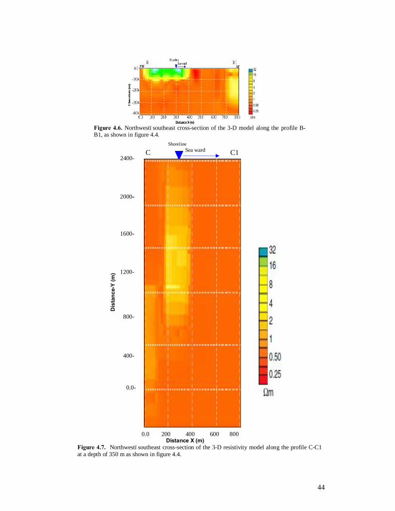
44

Figure 4.7. Northwest–southeast cross-section of the 3-D resistivity model along the profile C-C1 at a depth of 350 m as shown in figure 4.4.

Shoreline Sea ward C1

0.0 200 400 600 800

2400-

2000-

1600- 1200-

800-

400- 0.0-

Dis

tanc

e-Y

(m)

Distance X (m)

C

Figure 4.6. Northwest–southeast cross-section of the 3-D model along the profile B-B1, as shown in figure 4.4.

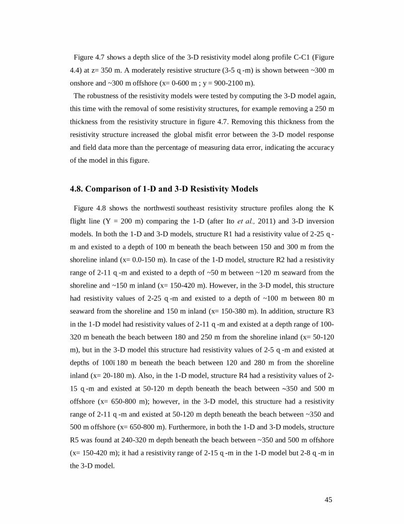
45

Figure 4.7 shows a depth slice of the 3-D resistivity model along profile C-C1 (Figure

4.4) at z= 350 m. A moderately resistive structure (3-5 Ω-m) is shown between ~300 m

onshore and ~300 m offshore (x= 0-600 m ; y = 900-2100 m).

The robustness of the resistivity models were tested by computing the 3-D model again,

this time with the removal of some resistivity structures, for example removing a 250 m

thickness from the resistivity structure in figure 4.7. Removing this thickness from the

resistivity structure increased the global misfit error between the 3-D model response

and field data more than the percentage of measuring data error, indicating the accuracy

of the model in this figure.

4.8. Comparison of 1-D and 3-D Resistivity Models

Figure 4.8 shows the northwest–southeast resistivity structure profiles along the K

flight line (Y = 200 m) comparing the 1-D (after Ito et al., 2011) and 3-D inversion

models. In both the 1-D and 3-D models, structure R1 had a resistivity value of 2-25 Ω-

m and existed to a depth of 100 m beneath the beach between 150 and 300 m from the

shoreline inland (x= 0.0-150 m). In case of the 1-D model, structure R2 had a resistivity

range of 2-11 Ω-m and existed to a depth of ~50 m between ~120 m seaward from the

shoreline and ~150 m inland (x= 150-420 m). However, in the 3-D model, this structure

had resistivity values of 2-25 Ω-m and existed to a depth of ~100 m between 80 m

seaward from the shoreline and 150 m inland (x= 150-380 m). In addition, structure R3

in the 1-D model had resistivity values of 2-11 Ω-m and existed at a depth range of 100-

320 m beneath the beach between 180 and 250 m from the shoreline inland (x= 50-120

m), but in the 3-D model this structure had resistivity values of 2-5 Ω-m and existed at

depths of 100–180 m beneath the beach between 120 and 280 m from the shoreline

inland (x= 20-180 m). Also, in the 1-D model, structure R4 had a resistivity values of 2-

15 Ω-m and existed at 50-120 m depth beneath the beach between ~350 and 500 m

offshore (x= 650-800 m); however, in the 3-D model, this structure had a resistivity

range of 2-11 Ω-m and existed at 50-120 m depth beneath the beach between ~350 and

500 m offshore (x= 650-800 m). Furthermore, in both the 1-D and 3-D models, structure

R5 was found at 240-320 m depth beneath the beach between ~350 and 500 m offshore

(x= 150-420 m); it had a resistivity range of 2-15 Ω-m in the 1-D model but 2-8 Ω-m in

the 3-D model.

46

Structure R6 showed resistivity of 2-11 Ω-m and existed at depths of 120-250 m

beneath the beach between ~350 and 500 m offshore (x= 650-800 m); this structure was

recovered only by the 3-D model results.

Overall, these figures show similar resistivity distributions, but with different

resistivity boundaries and values.

The main difference between the 1-D and 3-D inversion results is that the 1-D

computation assumed a layer structure and did not consider lateral resistivity change.

Since the computation processes of 1-D inversion assume horizontal layers that extend

to infinity, the conductor thickness and its contrast are too small to recover the observed

data at point by point. However, a 3-D inversion model reflects a real size, tends to have

larger conductor size, and its contrast better explains the observed values.

Figure 4.8. Northwest–southeast resistivity structure profiles along the K flight line (Y = 200 m), comparing (A) the 1-D inversion model (after Ito et al., 2011) and (B) 3-D model of current study. Color scale of 3-D model changed to fit the color scale used in Ito et al. (2011)

Ω.m

B)

A)

Dep

th-Z

(m)

Distance- X (m)

Shoreline Sea ward NW SE

300

200

100

0

400 100 200 500 600 700 800 300

400

0.0

R1 R4

R3

R2

R5

Source

R1

R3

R4

R6

R2

R5

Distance- X (m)

D

epth

-Z (m

)

47

4.9. Discussion The 3-D resistivity model results of the present study show that low resistivity (< 2 Ω-

m) is characteristic of most of the area beneath both land and sea. A landmass with high

resistivity (3-25 Ω-m) extends to a depth of ~100 m at 80 m seaward from the shoreline

to ~300 m inland. In addition, a resistive structure (3-10 Ω-m) exists to a depth of ~350

m beneath the beach 400-600 m seaward from the shoreline.

previous study in the same area for example, Uehara et al. (2007) found a highly

resistive landmass of 3-100 Ω-m extending to a depth of 40 m beneath the beach and

showed that low resistivity (< 2 Ω-m) is characteristic below the highly resistive

landmass and adjacent sea bottom. Hayashi et al. (2009) reported wellbore logging data

from 30 m to 1660 m depths adjacent to our study site (Figure 4.1). Those data indicated

that a low-resistivity zone of 1-2 Ω-m exists from 30 m to at least 1000 m in depth.

These previous studies were taken as an evidence present study results. Hence, the

following geological features were clarified in the study area. A high-resistivity

landmass (sandy ridge) exists down to a depth of ~100 m underlain by a low-resistivity

structure (Quaternary siltstone) which is characteristic of most of the study area beneath

both land and sea. In addition, a surficial low-resistivity structure (salt marsh) exists

behind the sandy ridge zone, which is thought to be caused by seawater intruding

through and beneath the ridges (Figure 4.6).

A near-surface 3-D conductor can cause a sign reversal if the conductor is between the

source and the receiver. If the receiver is between the conductor and the transmitter, the

voltage curve is shifted to higher amplitudes at early times due to lateral conductivity

variations in the surface time-domain EM (Hoerdt et al., 1992). Furthermore, the

vertical magnetic field has the largest sensitivity in the near-surface region between the

source and the receiver. These sensitivity distributions suggest that the received signals

are strongly affected by any anomaly existing between the source and the receiver

(Mitsuhata et al., 2002). This phenomenon is recognized in our results as shown in

figure 4.8. Namely, in comparison with the 1-D model, the 3-D model showed

resistivity structures of larger size that were shifted to depths of several tens of meters in

the land side close to the source area; this is attributable to the large electromagnetic

field sensitivity distribution in front of the source area. To verify our results I have

compared them with Mitsuhata et al. (2006)’s results where they reported that on the

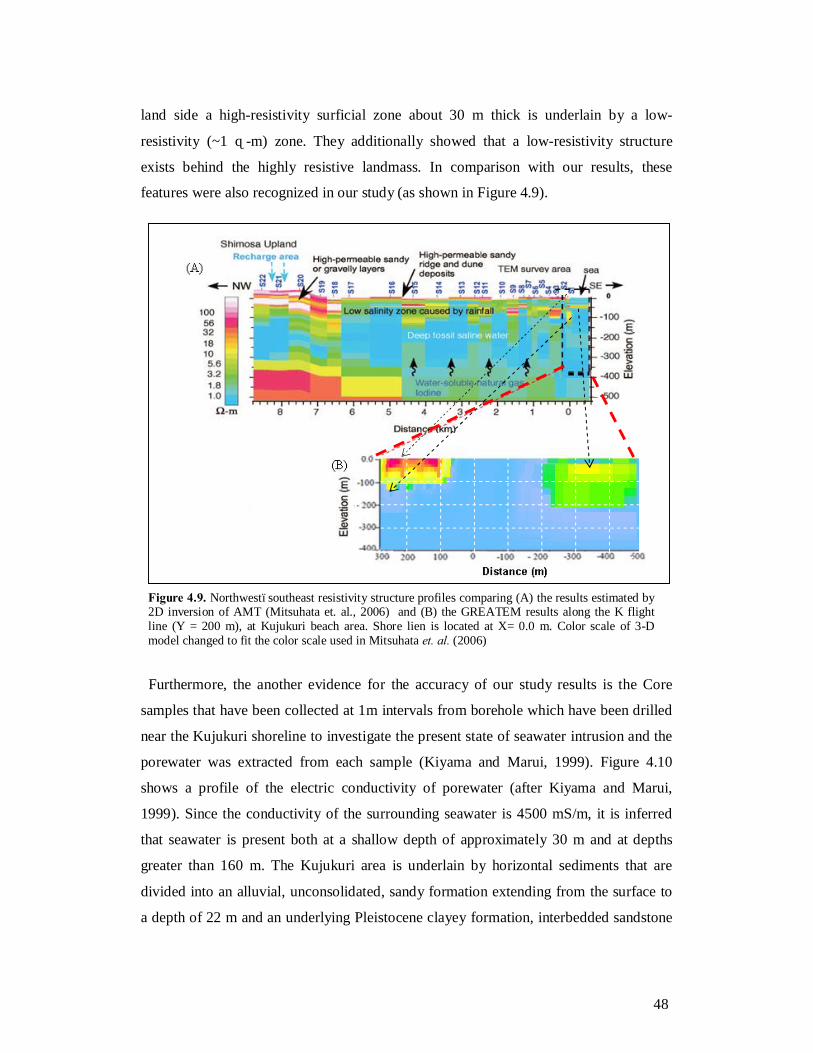
48

land side a high-resistivity surficial zone about 30 m thick is underlain by a low-

resistivity (~1 Ω-m) zone. They additionally showed that a low-resistivity structure

exists behind the highly resistive landmass. In comparison with our results, these

features were also recognized in our study (as shown in Figure 4.9).

Furthermore, the another evidence for the accuracy of our study results is the Core

samples that have been collected at 1m intervals from borehole which have been drilled

near the Kujukuri shoreline to investigate the present state of seawater intrusion and the

porewater was extracted from each sample (Kiyama and Marui, 1999). Figure 4.10

shows a profile of the electric conductivity of porewater (after Kiyama and Marui,

1999). Since the conductivity of the surrounding seawater is 4500 mS/m, it is inferred

that seawater is present both at a shallow depth of approximately 30 m and at depths

greater than 160 m. The Kujukuri area is underlain by horizontal sediments that are

divided into an alluvial, unconsolidated, sandy formation extending from the surface to

a depth of 22 m and an underlying Pleistocene clayey formation, interbedded sandstone

Figure 4.9. Northwest–southeast resistivity structure profiles comparing (A) the results estimated by 2D inversion of AMT (Mitsuhata et. al., 2006) and (B) the GREATEM results along the K flight line (Y = 200 m), at Kujukuri beach area. Shore lien is located at X= 0.0 m. Color scale of 3-D model changed to fit the color scale used in Mitsuhata et. al. (2006)

49

and mudstone. Permeability estimates have been made on the basis of core sample

measurements. This confirms the credibility of our 3-D models and the applicability of

the GREATEM method to coastal research.

4.10. Conclusions The present study results revealed that the GREATEM system can detect resistivity

structures in coastal areas down to a depth of ~350 m, within a distance of more than

500 m from the shoreline. The induced current just beneath the source is almost zero

and the penetration depth gradually increases with range on both sides of the source. As

a result, the GREATEM method has some limitations in that it is difficult to delineate

the resistivity structure directly beneath the source, but data quality worsens with

increasing distance from the source (Ito et al., 2011). However, the present results show

Figure 4.10. Pore-water conductivity profile measured from core samples extracted from borehole drilled near the Kujukuri shoreline (after Kiyama and Marui, 1999). (Modified from Mitsuhata et al., [2006].)

50

that the GREATEM system can be a useful tool for studying the characteristics of

sea/land boundaries in coastal areas.

The method is also a promising tool for modeling 3-D resistivity structures in coastal

areas such as the subterranean distribution of saline water which may lead to land slide

or collapse in a volcano edifies and cliff or steep slope along fault (Mogi et al., 2009),

as a result, this information can be useful for the study of earthquakes and tsunamis,

management of water resources, and development planning in coastal areas. Three-

dimensional resistivity modeling that considers large lateral resistivity variations is one

recommended solution for the large resistivity contrasts between land and sea in surveys

of coastal areas where a 1-D resistivity model that assumes a horizontally layered

structure might be inaccurate. Overall, 3-D models are better in recovering the

resistivity structures at all depths and can account for lateral conductivity variations.

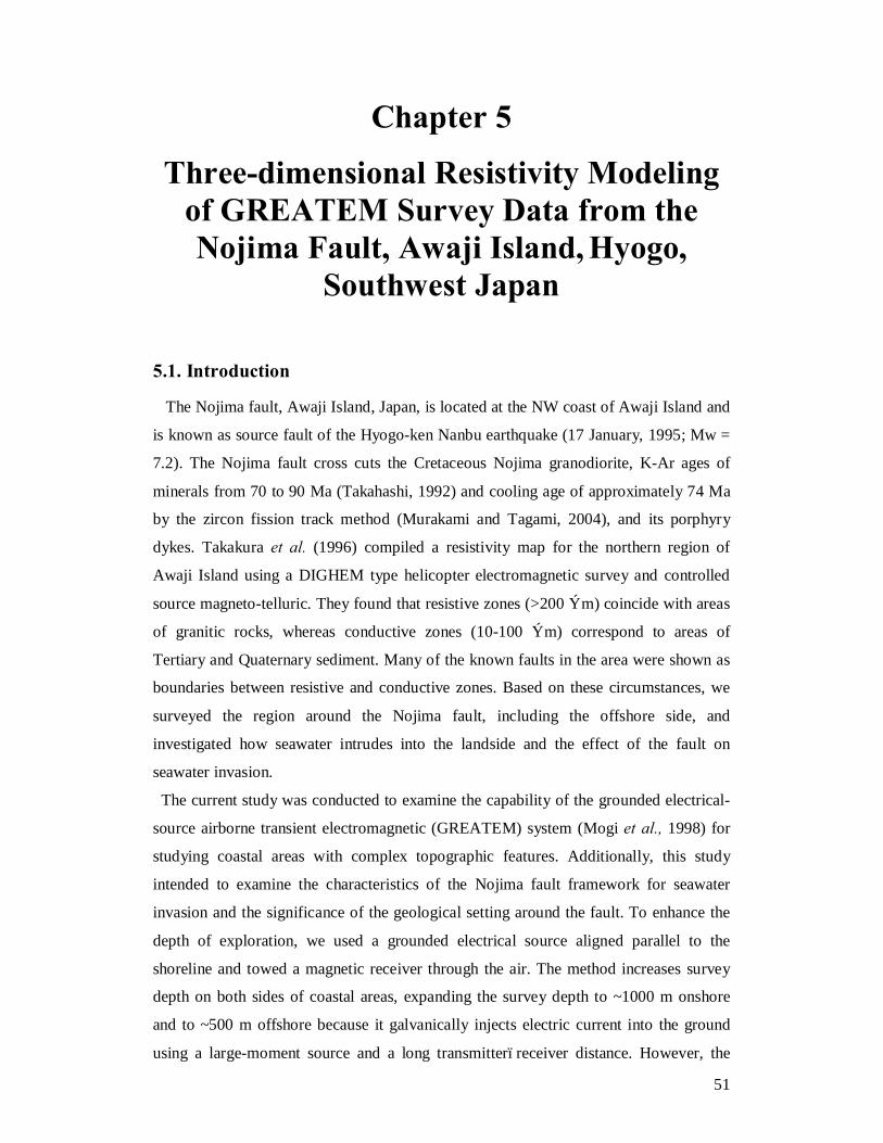
51

Chapter 5

Three-dimensional Resistivity Modeling of GREATEM Survey Data from the Nojima Fault, Awaji Island, Hyogo,

Southwest Japan 5.1. Introduction

The Nojima fault, Awaji Island, Japan, is located at the NW coast of Awaji Island and

is known as source fault of the Hyogo-ken Nanbu earthquake (17 January, 1995; Mw =

7.2). The Nojima fault cross cuts the Cretaceous Nojima granodiorite, K-Ar ages of

minerals from 70 to 90 Ma (Takahashi, 1992) and cooling age of approximately 74 Ma

by the zircon fission track method (Murakami and Tagami, 2004), and its porphyry

dykes. Takakura et al. (1996) compiled a resistivity map for the northern region of

Awaji Island using a DIGHEM type helicopter electromagnetic survey and controlled

source magneto-telluric. They found that resistive zones (>200 Ωm) coincide with areas

of granitic rocks, whereas conductive zones (10-100 Ωm) correspond to areas of

Tertiary and Quaternary sediment. Many of the known faults in the area were shown as

boundaries between resistive and conductive zones. Based on these circumstances, we

surveyed the region around the Nojima fault, including the offshore side, and

investigated how seawater intrudes into the landside and the effect of the fault on

seawater invasion.

The current study was conducted to examine the capability of the grounded electrical-

source airborne transient electromagnetic (GREATEM) system (Mogi et al., 1998) for

studying coastal areas with complex topographic features. Additionally, this study

intended to examine the characteristics of the Nojima fault framework for seawater

invasion and the significance of the geological setting around the fault. To enhance the

depth of exploration, we used a grounded electrical source aligned parallel to the

shoreline and towed a magnetic receiver through the air. The method increases survey

depth on both sides of coastal areas, expanding the survey depth to ~1000 m onshore

and to ~500 m offshore because it galvanically injects electric current into the ground

using a large-moment source and a long transmitter–receiver distance. However, the

52

depth of investigation by current conventional time domain AEM can reach up to 1200

m in case of resistive ground. This study represents the deepest investigation depth by

AEM in mapping the subsurface below shallow saline water in coastal areas; this is

because the relatively high conductivity of salt water decreases the penetration depth of

the AEM signal and tends to shield structures beneath it and often limits geophysical

information that can be extracted from the data (Kirkegaard et al., 2011) 5.2. Survey Area Description

Awaji Island, Hyōgo Prefecture, Japan, is located in the eastern part of the Seto Inland

Sea between the islands of Honshū and Shikoku as shown in figure 5.1. Many active

faults, such as the Nojima fault, Asano fault, Higashiura fault, Kunono fault,

Nakamochi fault, Kusumoto faults, and the active fault system of the Median Tectonic

Line, are known in the area from Kobe through Awaji Island to northeast Shikoku

(Research Group for Active Faults of Japan, 1991). These fault systems are considered

to have been active under an east–west compressive stress field since the middle

Quaternary (Okada, 1973; Oka and Sangawa, 1981; Sangawa, 1984; Mizuno et al.,

1990). The uplift of the Rokko Mountains and Awaji Island and the subsidence of

Osaka Bay are known in the Kinki District as the Rokko movement (Ikebe, 1956;

Huzita, 1980). A 10.5-km surface fault rupture, the Hokudan Surface Fault Rupture

System, appeared along the northwestern coast of Awaji Island after the 1995 Hyogo-

ken Nanbu earthquake (Awata et al., 1996). The surface rupture consists of a northeast–

southwest right-lateral fault system with a high-angle reverse component. The system

has two strands: the 8.8 km Nojima fault and the 3.0 km Ogura fault. Surface

displacement is prominent along the Ogura fault and the northern part of the Nojima

fault. The maximum displacement along the central part of the North Nojima fault

measures 2.5 m (2.1 m of right-lateral displacement and 1.3 m of vertical displacement)

(Awata et al., 1998). In contrast, the surface displacement is very small along the

southern part of the Nojima fault, where it is parallel with the Ogura fault.

5.3. Previous Geophysical Studies The geological setting consists principally of Cretaceous granite, which is extensively

exposed on the northern part of Awaji Island. Tertiary and Quaternary sediments crop

out around the granite near the coast and consist of alternating layers of silt, clay, sand,

and conglomerate. Some DC electric and electromagnetic surveys have previously been

53

completed along the Hokudan Surface Fault Rupture System, as reported by Koreishi et

al. (1996), Suzuki et al. (1996), Takahashi et al. (1996), Takakura et al. (1996), and the

Electromagnetic Research Group for the 1995 Hyogo-ken Nanbu Earthquake (1997).

These studies describe two-dimensional (2D) and three-dimensional (3-D) resistivity

surveys and very low-frequency magnetotelluric (VLF-MT) surveys in the regions of

Hirabayashi, Ogura, and Nashimoto. A resistivity boundary coincides with the surface

position of the fault in the Hirabayashi area.

Murata et al. (2001) described the stratigraphy and geological cross section along the

Disaster Prevention Research Institute, Kyoto University, 500 m borehole drilled into

the Nojima fault zone, along which a surface rupture occurred during the 1995 Hyogo-

ken Nanbu earthquake. They estimated the vertical component of the displacement and

the average slip rate of the Nojima fault based on a structural contour map of the

unconformity surface above the basement rocks.

Nishigami et al. (2001) deployed borehole seismometers at three depths inside and

outside the fault zone along the Disaster Prevention Research Institute, Kyoto

University, 1800 m borehole into the Nojima fault zone to estimate the fault zone

structure down to seismogenic depths by analysing seismic waves propagating through

the low-velocity fault zone, known as ‘fault zone-trapped waves’. The results revealed

that the width of the Nojima fault was approximately 20 m and that the velocity and

attenuation of S waves (Q value) were approximately 1.0 km/s and Q = 20 inside the

fault zone and 2.5 km/s and Q = 100 outside the fault zone, respectively. Yamaguchi et

al. (2001) reported the results of VLF-MT surveys, which were made just after ruptures

occurred, at six sites across the Hokudan surface fault rupture system to clarify the

shallow resistivity structures associated with the ruptures. Their results indicate that the

resistivity structure around the Hokudan earthquake system is related to the

morphological characteristics of the fault and that conductive zones occur along the

faults where surface displacement is prominent. Lin et al. (2007) conducted a drilling

project through the Nojima fault zone, Awaji Island, to document the effects of the 1995

M7.2 Kobe earthquake recorded within the fault zone. They concluded that the Nojima

fault zone contains a damage zone characterized by a network of subsidiary faults and

fractures adjacent to the main fault.

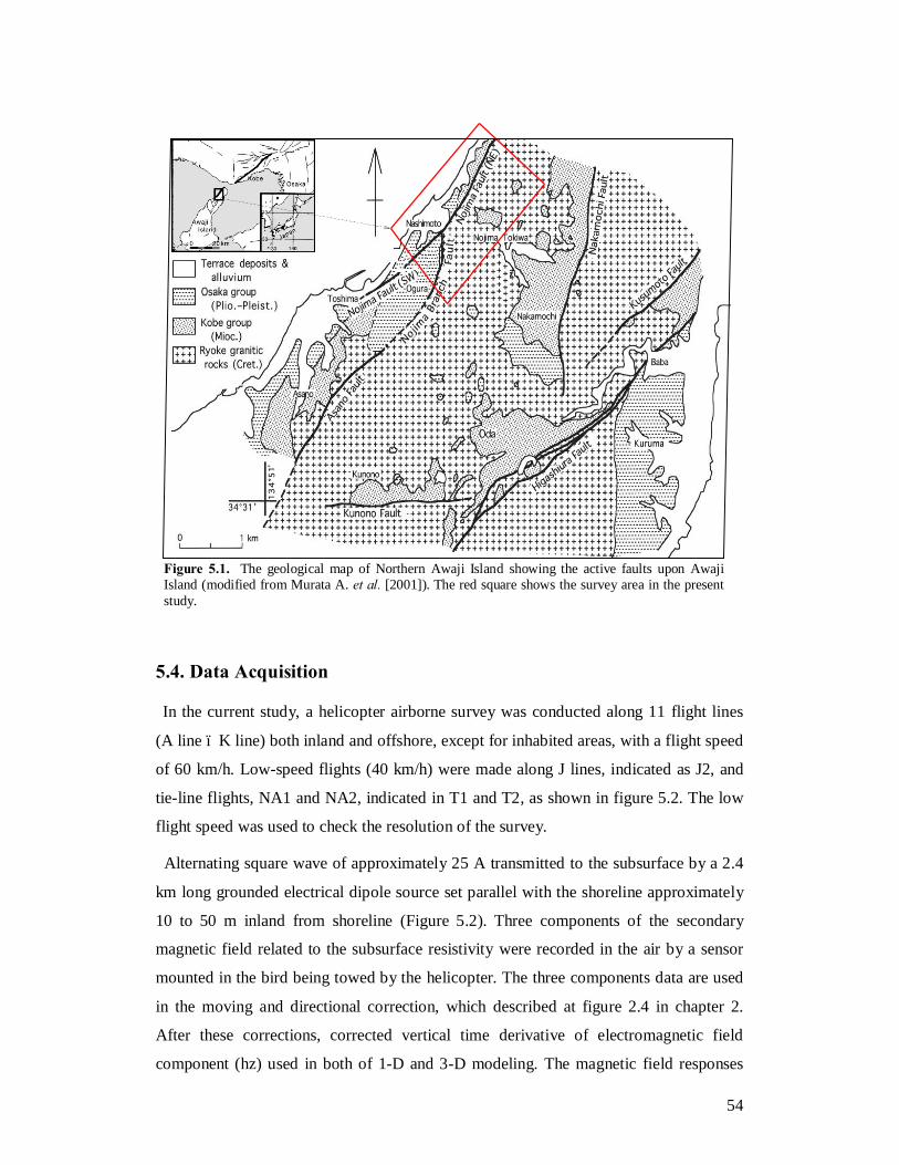
54

5.4. Data Acquisition

In the current study, a helicopter airborne survey was conducted along 11 flight lines

(A line – K line) both inland and offshore, except for inhabited areas, with a flight speed

of 60 km/h. Low-speed flights (40 km/h) were made along J lines, indicated as J2, and

tie-line flights, NA1 and NA2, indicated in T1 and T2, as shown in figure 5.2. The low

flight speed was used to check the resolution of the survey.

Alternating square wave of approximately 25 A transmitted to the subsurface by a 2.4

km long grounded electrical dipole source set parallel with the shoreline approximately

10 to 50 m inland from shoreline (Figure 5.2). Three components of the secondary

magnetic field related to the subsurface resistivity were recorded in the air by a sensor

mounted in the bird being towed by the helicopter. The three components data are used

in the moving and directional correction, which described at figure 2.4 in chapter 2.

After these corrections, corrected vertical time derivative of electromagnetic field

component (hz) used in both of 1-D and 3-D modeling. The magnetic field responses

Figure 5.1. The geological map of Northern Awaji Island showing the active faults upon Awaji Island (modified from Murata A. et al. [2001]). The red square shows the survey area in the present study.

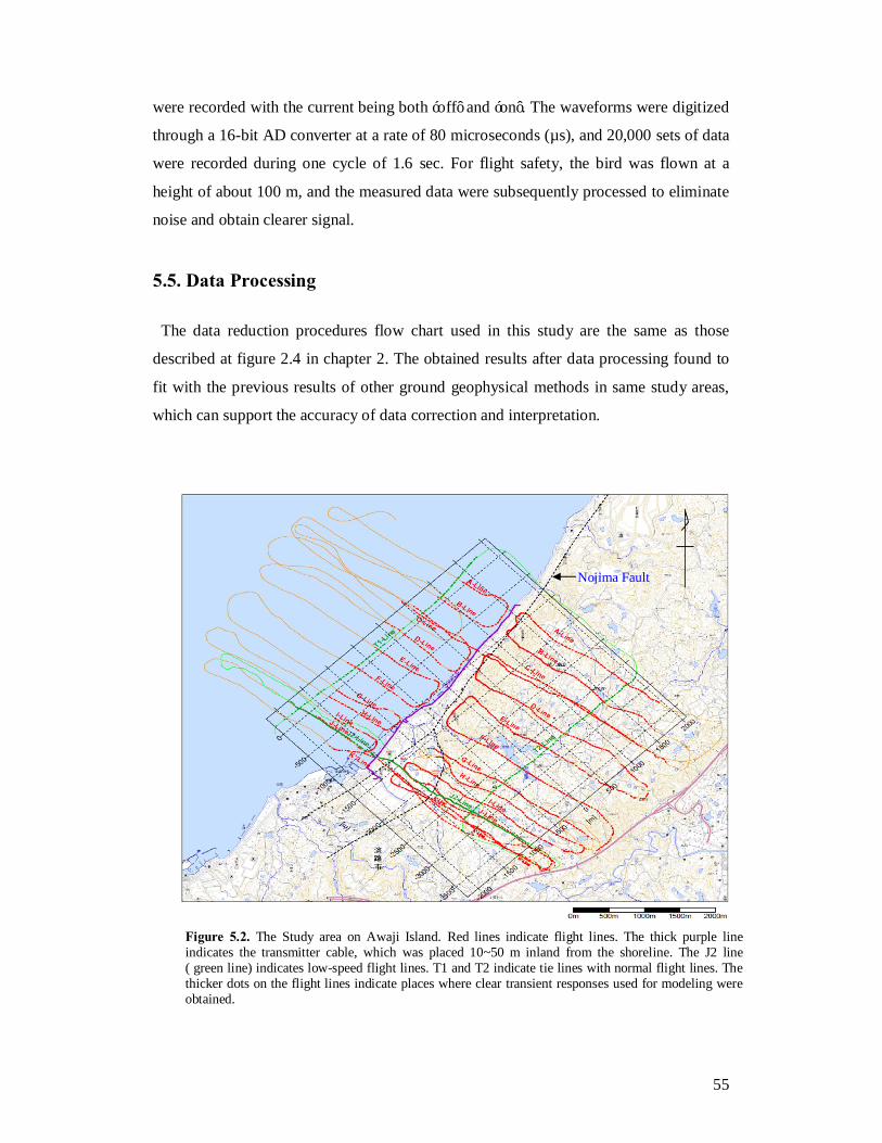
55

were recorded with the current being both ‘off’ and ‘on’. The waveforms were digitized

through a 16-bit AD converter at a rate of 80 microseconds (µs), and 20,000 sets of data

were recorded during one cycle of 1.6 sec. For flight safety, the bird was flown at a

height of about 100 m, and the measured data were subsequently processed to eliminate

noise and obtain clearer signal.

5.5. Data Processing

The data reduction procedures flow chart used in this study are the same as those

described at figure 2.4 in chapter 2. The obtained results after data processing found to

fit with the previous results of other ground geophysical methods in same study areas,

which can support the accuracy of data correction and interpretation.

Nojima Fault

Figure 5.2. The Study area on Awaji Island. Red lines indicate flight lines. The thick purple line indicates the transmitter cable, which was placed 10~50 m inland from the shoreline. The J2 line ( green line) indicates low-speed flight lines. T1 and T2 indicate tie lines with normal flight lines. The thicker dots on the flight lines indicate places where clear transient responses used for modeling were obtained.

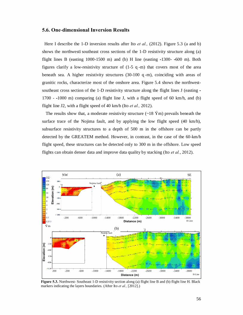
56

5.6. One-dimensional Inversion Results

Here I describe the 1-D inversion results after Ito et al., (2012). Figure 5.3 (a and b)

shows the northwest–southeast cross sections of the 1-D resistivity structure along (a)

flight lines B (easting 1000-1500 m) and (b) H line (easting -1300- -600 m). Both

figures clarify a low-resistivity structure of (1-5 Ω-m) that covers most of the area

beneath sea. A higher resistivity structures (30-100 Ω-m), coinciding with areas of

granitic rocks, characterize most of the onshore area. Figure 5.4 shows the northwest-

southeast cross section of the 1-D resistivity structure along the flight lines J (easting -

1700 - -1000 m) comparing (a) flight line J, with a flight speed of 60 km/h, and (b)

flight line J2, with a flight speed of 40 km/h (Ito et al., 2012).

The results show that, a moderate resistivity structure (~18 Ωm) prevails beneath the

surface trace of the Nojima fault, and by applying the low flight speed (40 km/h),

subsurface resistivity structures to a depth of 500 m in the offshore can be partly

detected by the GREATEM method. However, in contrast, in the case of the 60-km/h

flight speed, these structures can be detected only to 300 m in the offshore. Low speed

flights can obtain denser data and improve data quality by stacking (Ito et al., 2012).

Figure 5.3. Northwest- Southeast 1-D resistivity section along (a) flight line B and (b) flight line H. Black markers indicating the layers boundaries. (After Ito et al., [2012].)

Ωm

H-Line

Elev

atio

n (m

)

Distance (m) 200 -200 -600 -1000 -1400 -1800 -2200 -2600 -3000 -3400 -3800

Nojima fault

(b)

NW SE

B-Line Distance (m) -200 -600 -1000 -1400 -1800 -2200 -2600 -3000 -3400 -3800

Elev

atio

n (m

)

Nojima fault

(a)

57

1-D models based on horizontal layers are adequate in many exploration situations,

but there are numerous cases such as large resistivity contrast boundaries where 3-D

modeling is required (Hoerdt et al., 1992). In this study, the results of 1-D inversion

assuming a horizontally layered structure found to fit with the field data, thus the 1-D

results are correct under this assumption, however, this is practically not a true case as

the subsurface structures are three-dimensional by nature. As a result, in comparison

with the resistivity values revealed by other studies in the same area however, the

offshore resistivity values revealed by 1-D inversion in present study were acceptable,

the onshore resistivity values were found to be much less than the values revealed by

these studies. This occurred because the sea has high conductivity, and the lateral

conductivity change effects on EM field induction were seriously large at the time of the

survey in the coastal area where the source cable was set very close to the shoreline (10-

50 m) due to the nature of the mountains and roads in the survey area and there was an

appropriate space far from sea. Abd Allah et al. (2013a) and discussed at chapter 3

reported the sea effect on EM field induction by GREATEM surveys at coastal areas.

They showed that, the sea effect when the source is located 10 m or 20 m landward

from the shoreline is much greater than when the source is 300 m from the shoreline.

Figure 5.4. Northwest- Southeast 1-D resistivity section along the J flight lines comparing (a) the J flight line with a flight speed of 60 km/h and (b) the J2 flight line with a flight speed of 40 km/h. Black markers indicating the layers boundaries. (After Ito et al., [2012].)

Ωm (b)

600 200 -200 -600 -1000 -1400 -1800 -2200 -2600 -3000 -3400

Elev

atio

n (m

)

Distance (m) J2-line

Flight speed (40km/h)

Distance (m) J-line

Flight speed (60km/h)

NW SE

200 -200 -600 -1000 -1400 -1800 -2200 -2600 -3000 -3400 -3800

(a)

Elev

atio

n (m

)

58

Therefore, the motivation of this study was to overcome the problem raised by 1-D

inversion results through generating a 3-D resistivity model that reflects a real size and

tends to have larger conductor size and its contrast to explain observed value, as

described in the following sections.

5.7. Three-dimensional Modeling of GREATEM Nojima Field Data

The modified staggered-grid finite-difference method developed by Fomenko and

Mogi (2002) and Mogi et al. (2011) which is described in the chapter 2 was used to

generate a 3-D resistivity structure model of the GREATEM system data from our study

area. As shown in figure 5.2, the survey covered a 4 x 4 km square area. The total model

size was x: 35 39 x z: 25 km with a 3-D model domain of x: 10 x y: 11 x z: 1.4 km. The

model size was gridded into x: 48 x y: 57 x z: 35 blocks. In the vertical direction, the

size of each grid varied from 5 m at the surface to 6400 m at the top and bottom of the

model. The horizontal size was approximately 200 m in the modeling area, and large-

sized (800~6400 m) grids were added at the circumference of the modeling area to

avoid an edge effect. The 3-D model was based on an initial model that consisted of two

adjacent onshore and offshore layers of different conductivity, in which a high

conductor sea of (10-40 m) depth is placed on top of a sedimentary rocks of varied low

resistivity, assuming the presence of a section of topographic structures placed on top of

high resistivity granitic rock on the inland side. The offshore resistivity values of the

starting initial model were based on the 1-D inversion results. Figure 5.5 shows a

section of the model.

The field data were stacked within each grid so that some 3-D effects due to small

surface reliefs were averaged out in this grid scale. The transient response curves of the

field data were fitted to those computed at the centre of each grid from the 3-D model. I

used trial and error methods, so the resistivity values of the initial model were

repeatedly changed to obtain the best fit between the 3-D synthetic model and the field

data. In the case of the field survey, 10,000 sets of data, digitized at a rate of 80

microseconds (µs), were obtained during a half cycle of 0.8 sec. In the case of the

numerical modeling, I used computed transient responses at 30 time channels and 10

time-equal spaces of a log scale in one decade, in the range of 100 microseconds (µs) to

100 milliseconds (ms) (3 decades).

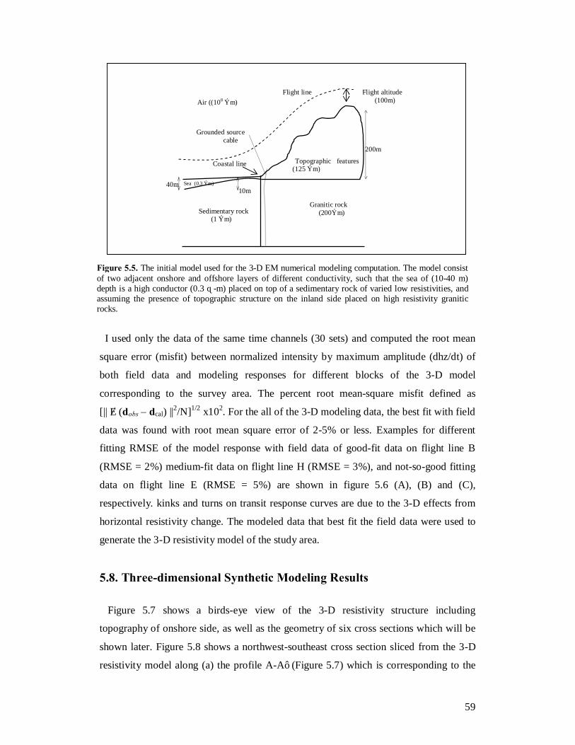
59

I used only the data of the same time channels (30 sets) and computed the root mean

square error (misfit) between normalized intensity by maximum amplitude (dhz/dt) of

both field data and modeling responses for different blocks of the 3-D model

corresponding to the survey area. The percent root mean-square misfit defined as

[|| Σ (dobs – dcal) ||2/N]1/2 x102. For the all of the 3-D modeling data, the best fit with field

data was found with root mean square error of 2-5% or less. Examples for different

fitting RMSE of the model response with field data of good-fit data on flight line B

(RMSE = 2%) medium-fit data on flight line H (RMSE = 3%), and not-so-good fitting

data on flight line E (RMSE = 5%) are shown in figure 5.6 (A), (B) and (C),

respectively. kinks and turns on transit response curves are due to the 3-D effects from

horizontal resistivity change. The modeled data that best fit the field data were used to

generate the 3-D resistivity model of the study area.

5.8. Three-dimensional Synthetic Modeling Results

Figure 5.7 shows a birds-eye view of the 3-D resistivity structure including

topography of onshore side, as well as the geometry of six cross sections which will be

shown later. Figure 5.8 shows a northwest-southeast cross section sliced from the 3-D

resistivity model along (a) the profile A-A’ (Figure 5.7) which is corresponding to the

Figure 5.5. The initial model used for the 3-D EM numerical modeling computation. The model consist of two adjacent onshore and offshore layers of different conductivity, such that the sea of (10-40 m) depth is a high conductor (0.3 Ω-m) placed on top of a sedimentary rock of varied low resistivities, and assuming the presence of topographic structure on the inland side placed on high resistivity granitic rocks.

Sea (0.3 Ωm)

200m

Topographic features (125 Ωm)

40m 10m

Granitic rock (200Ωm) Sedimentary rock

(1 Ωm)

Flight altitude (100m)

Coastal line

Flight line

Grounded source cable

Air ((108 Ωm)

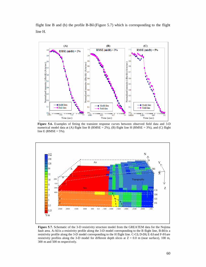
60

flight line B and (b) the profile B-B’ (Figure 5.7) which is corresponding to the flight

line H.

Time (sec) Time (sec)

Nor

mal

ized

inte

nsity

(dh

z/dt

) (A

/m/s

ec)

Nor

mal

ized

inte

nsity

(dhz

/dt)

(A/m

/sec

)

Nor

mal

ized

inte

nsity

(dh

z/dt

) (A

/m/s

ec)

Time (sec)

C

Figure 5.6. Examples of fitting the transient response curves between observed field data and 3-D numerical model data at (A) flight line B (RMSE = 2%), (B) flight line H (RMSE = 3%), and (C) flight line E (RMSE = 5%).

(B) (C) (A)

Z

X

Y

2500 2000 1500 1000 500 0.0 - 500 -1000 -1500 -2000 -2500 -3000 -350

200-

0.0-

200-

400-

-2000

0.0

2000

N

E

A B’

B

C

C’

D’

E’

F’

D

F

A Air

Sea

Topography

Ωm

Figure 5.7. Schematic of the 3-D resistivity structure model from the GREATEM data for the Nojima fault area. A-A’ is a resistivity profile along the 3-D model corresponding to the B flight line, B-B’ is a resistivity profile along the 3-D model corresponding to the H flight line. C-C’, D-D’, E-E’ and F-F’ are resistivity profiles along the 3-D model for different depth slices at Z = 0.0 m (near surface), 100 m, 300 m and 500 m respectively.

61

The results indicate that a highly conductive layer (<10 Ω-m) is dominant beneath the

sea in both of the offshore and coastal areas and extends to the Nojima fault at levels

deeper than several meters. The onshore area is characterized by high-resistivity

structures (100-300 Ω-m) coinciding with areas of granitic rocks, in addition to a

moderate resistivity structure (50-75 Ω-m), which can be interpreted as a sedimentary

deposit. A conductive structure with a resistivity of (10-30 Ωm) was also revealed

beneath the surface trace of the fault. These models are able to reflect the clear

resistivity contrast between the sedimentary and granitic rock which is expected,

however there is another resistivity contrast in the onshore area between the structures

above sea level and those are below sea level, the reason for that is unknown.

Figure 5.9 (A, b, C and D) shows a plan view of the 3-D resistivity model at different

depth slices, along the profile C-C’, D-D’, E-E’ and F-F’ (Figure 5.7) at Z = 0.0 m (near

surface), 100 m, 300 m and 500 m respectively. As can be seen, from the surface to 500

Figure 5.8. Northwest–southeast cross section of the 3-D resistivity model, (a) along A-A’ profile (Figure 5.7) which corresponding to flight line B and (b) B-B’ profile (Figure 5.7) which corresponding to flight line H.

Shoreline Sea ward

Nojima fault

SE NW (a)

600 200 -200 -600 -1000 -1400 -1800 -2200 -2600 -3000 -3400

-200-

0.0- -200- -400-

Distance (m)

Elev

atio

n (m

)

Ωm

Distance (m)

Elev

atio

n (m

)

600 200 -200 -600 -1000 -1400 -1800 -2200 -2600 -3000

(b)

-200-

0.0- -200- -400-

Elev

atio

n (m

)

Shoreline Sea ward

A A’

B B’

62

m, a highly conductive layer (< 10 Ω-m) is dominant in the offshore area. In contrast, a

highly resistive layer (50-500 Ω-m), which coincides with granitic rock and embedded

sedimentary deposits, is dominant in the onshore area. The resistivity structure is almost

uniform along the fault, but some resistivity variation is seen in the direction

perpendicular to the fault strike. The Nojima fault is located at a clear resistivity

structure boundary and acts as barrier to sea water invasion.

The robustness of the resistivity models were tested by computing the 3-D models

again, this time with the removal of some resistivity structures, for example removing a

200 m thickness from the offshore resistivity structure (x= -500 - -700 m) showed in the

figure 5.8(a). Removing this thickness from the resistivity structure has significantly

increased the global misfit error between the 3-D model response and field data, more

than the percentage of measuring data error, indicating the accuracy of the model in

these figures.

5.9. Comparison of 1-D and 3-D Resistivity Models Figure 5.10 shows the northwest–southeast resistivity structure profiles along the B

flight line comparing (a) the 1-D and (b) the 3-D inversion models. As we can see, the

results of both the 1-D inversion and 3-D resistivity models in the current study clarified

that a resistivity structure (~1 Ω-m) is dominant in the offshore area beneath the sea. In

Figure 5.9. (A), (B), (C) and (D) are Plan view of 3-D resistivity model at different depth slices along profiles C-C’, D-D’, E-E’ and F-F’ (Figure 5.7) at different depth slices at Z = 0.0 m (near surface), 100 m, 300 m and 500 m respectively.

’

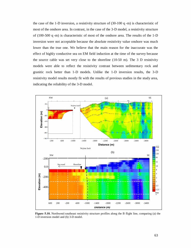
63

the case of the 1-D inversion, a resistivity structure of (30-100 Ω-m) is characteristic of

most of the onshore area. In contrast, in the case of the 3-D model, a resistivity structure

of (100-500 Ω-m) is characteristic of most of the onshore area. The results of the 1-D

inversion were not acceptable because the absolute resistivity value onshore was much

lower than the true one. We believe that the main reason for the inaccurate was the

effect of highly conductive sea on EM field induction at the time of the survey because

the source cable was set very close to the shoreline (10-50 m). The 3 D resistivity

models were able to reflect the resistivity contrast between sedimentary rock and

granitic rock better than 1-D models. Unlike the 1-D inversion results, the 3-D

resistivity model results mostly fit with the results of previous studies in the study area,

indicating the reliability of the 3-D model.

Figure 5.10. Northwest–southeast resistivity structure profiles along the B flight line, comparing (a) the 1-D inversion model and (b) 3-D model.

SE NW

Distance (m) -200 -600 -1000 -1400 -1800 -2200 -2600 -3000 -3400 -3800

Elev

atio

n (m

)

Nojima fault

(a)

Ω.mm

Shoreline coastline

Sea ward

Nojima fault

Distance (m)

SE NW (b)

600 200 -200 -600 -1000 -1400 -1800 -2200 -2600 -3000 -3400

-200-

0.0- -200- -400- E

leva

tion

(m)

64

5.10. Discussion

The 3-D results of the present study clarified that a low-resistivity structure (1-5 Ω-m)

is characteristic of most of the offshore area beneath the sea. A moderate-resistivity

structure (~25 Ω-m) is characteristic of the coastal zone between the offshore and

onshore areas. Highly resistive zones (100-300 Ω-m) coincide with areas of granitic

rocks and are characteristic of most of the onshore area.

Previous studies in the same area showed that the inland side of the Nojima fault is

resistive (>200 Ωm) and that the coastal side is conductive (10~100 Ωm) (Takakura et

al., 1996). DC surveys in the Nashimoto area by Koreishi et al. (1996) and Suzuki et al.

(1996) revealed an uppermost layer that is moderately resistive (100~200 Ωm) and

about 10 m thick. A moderately conductive dyke structure with a resistivity of (30~60

Ωm) was also revealed just beneath the surface trace of the Nojima fault.

These previous studies were taken as evidence for reasonable interpretations of the

present study results. Hence the following geological features can be clarified in the

study area. A highly conductive zone of (1-3 Ωm), coinciding with Paleogene and

Quaternary sedimentary rock, consisting of alternating layers of silt, clay, and sand is

characteristic of the offshore area beneath the sea. A highly resistive zone of (>200 Ωm)

coinciding with granitic rock is characteristic of the onshore area. The Nojima fault acts

as a barrier to seawater invasion in the area, as can be seen in Figures 5.8 and 5.9. At

very shallow depths (Figure 5.9 A), highly conductive structure which can be

interpreted as seawater because it has the same resistivity values of seawater found

offshore area, intrudes into the landside area up to the fault zone. At a depth of about

100 m (Figure 5.9 B), less-conductive sedimentary deposits occur in the coastal area. At

a depth of about 200 m (Figure 5.8 A), seawater appears to again invade the landside

area. Furthermore, an offshore conductive structure (~5 Ωm) appears to invade the

landside at deeper level of 300 and 500 m (Figure 5.9 C and D).

To verify our results I have compared them with the Takakura et al. (1996) result in

which they compiled a resistivity map of the northern region of Awaji Island from a

helicopter electromagnetic and array controlled source audio frequency magnetotellurics

(CSAMT) investigation. They found that resistive zones (200 -1000 Ωm) coincide with

areas of granitic rocks and that conductive zones (10 -100 Ωm) correspond to areas of

paleogene and Quaternary sediments. In comparison with these results as shown in

figure 5.11, however the GREATEM results don't recover exact resistivity values of

65

their study, but in general both of conductive features (< 100 Ω-m) and resistive

features (>500 Ωm) were also recognized in our GREATEM results.

Although the GREATEM’ 3-D resistivity model results have been improved in

comparison with 1-D models results and they overall can reflect the subsurface structure

of the area nearly as shown by CSAMT results (Takakura et al. 1996) but, their

resistivity values are not completely fit with the values reveled by CSAMT study, this

maybe because the resistivity section showed by Takakura et al. (1996) is located at 1-

km northern the B line of our results. Also, maybe due to the effect of high conductive

sea on magnetic field induction by GREATEM was large because the source location

was very close to shoreline (Abd Allah et al., 2013a). Furthermore, the measured data

density of GREATEM is much more than CSAMT case which maybe also anther

reason.

Figure 5.11. Northwest–southeast resistivity structure profiles comparing (A) the results of CSAMT (Takakura et. al., 1996) and (B) the GREATEM results along the B flight line at Awaji Island. Coast line is at X=0 m. Color scale of 3-D model changed to fit the color scale used in Takakura et al. (1996)

200-

0.0-

-200- -400-

0.0 500 1000 1500 2000 2500

Distance (m)

Elev

atio

n (m

) El

evat

ion

(m)

Distance (km)

(B)

(A)

Ω-m

66

Furthermore, I have compared my results with the Ikeda et al. (2000) result in which

they showed a resistivity sections of the northern region of Awaji Island from CSAMT

investigation. They found that, in the shallower part there is a resistive zones (50 -500

Ωm) coincide with areas of granitic rocks and that conductive zones (10 -200 Ωm) close

to the area of Nojima fault. In comparison with these results as shown in figure 5.12, in

general both of conductive features (< 100 Ω-m) and resistive features (>200 Ωm) were

also recognized in our GREATEM results. Both of (A) and (B) sections are located

close to each other. It should be mentioned that, in case of CSAMT results (A) there is

only a few measuring point, so maybe the sensitivity of the GREATEM results (B) is

much better due to the dense of the measuring points.

Another evidence for the accuracy of our results is clarified in the figure 5.13, which

shows the resistivity wellbore logging data from 250 m to 2000 m depths by Ikeda et al.,

(2000) adjacent to our study site (Figure5.2). Their data indicated that a high-resistivity

zone of value ranging from 200 - 3000 Ω-m exists from 250 m to at least 1800 m in

Nojima cross sectional

Figure 5.12. Northwest–southeast resistivity structure profiles comparing (A) the results of CSAMT (Ikeda et. al., 2000) and (B) the GREATEM results along the B flight line at Awaji Island. Coast line is at X=0 m. Color scale of 3-D model changed to fit the color scale used in Ikeda et al. (2000)

(A)

(B)

Ω-m

67

depth. At a depth of 300 m the results raveled a resistivity structure (200- 2000 Ω-m)

which also revealed by our results at the same depth.

5.11. Conclusions

In the current study, I obtained a reasonable 3-D resistivity structure around the

Nojima fault, which runs along the shoreline. Our results delineated how seawater

invades the landside and revealed the fault is a barrier to seawater invasion.

Unlike 1-D resistivity models, the 3-D resistivity model can provide accurate and

reliable data, especially at coastal areas where the sea effect on EM induction is

significant. The present results show that the GREATEM system can be a useful tool for

studying the characteristics of coastal areas with complex topographic features to a

depth of several hundred meters. The method is also a promising tool for modeling 3-D

resistivity structures in coastal areas, such as sand ridges and subterranean distributions

Resistivity (Ω-m)

Dep

th (m

)

Nojima Cross-sectional

Figure.5.13. Resu1ts of the boreho1e e1ectrica1 resistivity logging data obtained from well drilling close Nojima fault area. (After Ikeda et al., [2000].)

68

of saline water. The results reflected that GREATEM can reveal the resistivity structure

of the Nojima fault running along coastal areas and this can be useful for delineating a

subsurface structure and characterization of an active fault under these situations. As

results, this information can be used for the mitigation of natural disasters such as

earthquakes and tsunamis, for the management of water resources, and for development

and planning in coastal areas.

The current study results fit well with the results of previous studies on Awaji Island,

confirming the credibility of 3-D models and assuring the applicability of our method to

coastal research. A 3-D resistivity modeling that considers large lateral resistivity

variations is required in case of large resistivity contrasts between land and sea in

surveys of coastal areas where 1-D resistivity model that assumes a horizontally layered

structure might be inaccurate.

69

Chapter 6

Summary and Future Plans

As a summary of this thesis, the GREATEM geophysical surveys and their 3-D

modeling have been shown to be effective in various environmental applications

performed at coast and active faults. With an improved signal-to-noise ratio and

stronger dipole moments of the transmitters, the variety of GREATEM surveys can be

expanded to study groundwater problems and mineral exploration. Conclusions of this

thesis are summarized in the following points:

1. I have verified our computing scheme, which is based on the 3-D SFD method

(Fomenko and Mogi, 2002) by comparing the results of a quarter-space and

trapezoidal hill models with the results of the 2.5-D FEM method developed by

Mitsuhata (2000), and the 3-D SLDM developed by Druskin and Knizhnerman (1994).

Although minor differences arise, the main features of the results obtained from the

three methods were similar. This confirms the accuracy and credibility of our

computing method.

2. The 3-D EM synthetic modeling results in this study indicate that the effect of the

sea on GREATEM survey data is inversely proportional to both the distance of the

dipole source from the shoreline and host-rock conductivity. Topography with high

slope angles has a greater effect than topography with low slope angles. In addition,

the area of the topographic feature closest to the dipole source has a large effect on

EM field induction for several meters. The modeling results of this study will be

considered when planning future GREATEM surveys, and will be used to provide a

reasonable interpretation of data collected in coastal areas. Although it is encouraging

that more studies of the effects of sea are supported by quantitative modeling, the non-

uniqueness of EM interpretation is a persistent problem, and modeling still has to rely

heavily on an obvious presumed structure.

3. The GREATEM field survey results at Kujukuri beach revealed that the system

can detect resistivity structures in coastal areas to a depth of ~350 m, within a distance

of more than 500 m from the shoreline. The induced current just beneath the source is

almost zero and the penetration depth increases gradually with range on both sides of

the source. As a result, the GREATEM method has some limitations in that it is

difficult to delineate the resistivity structure directly beneath the source, but data

70

quality deteriorates with increasing distance from the source (Ito et al., 2011).

However, the present results show that the GREATEM system can be useful for

studying the characteristics of sea/land boundaries in coastal areas. The method is also

promising for modeling 3-D resistivity structures in coastal areas, such as the

subterranean distribution of saline water, which can lead to landslides or collapse in

volcanic edifices and cliffs or steep slopes along faults (Mogi et al., 2009). As a result,

this information can be useful for the study of earthquakes and tsunamis, management

of water resources, and development planning in coastal areas.

4. The results of the second GREATEM field survey at Nojima fault, Awaji Island,

were used to delineate a reasonable 3-D resistivity structure around the Nojima fault,

which runs along the shoreline. Our results explained how seawater invades the

landside. Unlike 1-D resistivity models, 3-D resistivity models can provide accurate

and reliable data, especially in coastal areas where the effect of the sea on EM

induction is significant. These results indicate that the GREATEM system can be a

useful tool for studying the characteristics of coastal areas with complex topographic

features to a depth of several hundred meters. The method is also a promising tool for

modeling 3-D resistivity structures in coastal areas, such as the subterranean

distribution of saline water. The information can be used for the mitigation of natural

disasters such as earthquakes and tsunamis, the management of water resources, and

development and planning in coastal areas. The results agree with the results of

previous studies on Awaji Island, confirming the credibility of 3-D models, and

confirming the applicability of our method to coastal research. Three-dimensional

resistivity modeling that considers large lateral resistivity variations is required where

large resistivity contrasts occur between the land and sea in surveys of coastal areas

where a 1-D resistivity model that assumes a horizontally layered structure might be

inaccurate.

5. Overall, 3-D models are better for recovering resistivity structures at all depths, and

can account for variations in lateral conductivity.

6. Finally, the results show that GREATEM system can give information regarding

seawater intrusion in sedimentary rocks and resistivity structure along active faults.

These results indicate that GREATEM is a promising method for the assessment of

natural disaster areas, such as earthquakes, volcanoes, and active faults, in addition to

natural resource management.

71

Through this research, I would like to propose some future projects that can develop

and improve the GREATEM system to increase its efficiency and applicability in

various types of research project. Because current 1-D inversion can be distorted in

some cases of surveying coastal areas, one research challenge is to complete

development of the 3-D EM inversion algorithm for interpreting GREATEM field

survey data in other areas with more complex topography (e.g., the Tokachidake

volcano, and the Nojima fault area). However, completion of development of this new

inversion code is challenging, because little significant research has been conducted

relative to the 3-D inversion of Airborne EM systems, but it will make a considerable

contribution to that field of study. Furthermore, other research plans include more

research studies aiming to improve and develop the GREATEM system, such as

increasing the transmitter source moment, as some heli-TEM systems now use a

moment of ~106 Am2. This, together with advanced modeling and inversion

procedures, can produce quantitative results useful for groundwater modeling in

coastal areas, which will expand application of the GREATEM system to

investigation of hazardous waste and seawater incursions, and facilitate its use in

hydrocarbon exploration.

72

List of Related Publications (A) Results Described in Chapter 3. 1. Abd Allah Sabry, Toru Mogi and Elena Fomenko, 2013a, Three-dimensional

electromagnetic modeling study of sea and topography effects on EM field

induction by grounded electrical source airborne transient electromagnetics

(GREATEM) system surveys, Proceedings of the 3-DEM5th international

symposium, Sapporo, Japan, May, 2013.

2. Mogi Toru, Elena Fomenko and Sabry Abd Allah, 2011, Three-dimensional

modeling of GREATEM data and its application to field data, Proceedings of

workshop on recent advances in ground and airborne electromagnetics methods -

innovation in processing and inversion techniques. AMD, India, September,

2011

(B) Results Described in Chapter 4. 3. Abd Allah Sabry, Toru Mogi, Hisatoshi Ito, Kazuhiro Tsukuda, Kenzo Kiho,

Hideshi Kaieda, Koichi Suzuki, Akira Jymori, Youichi Yuuki and Elena

Fomenko, 2013b, Three-dimensional resistivity characterization of a coastal area:

application to the Grounded Electrical-Source Airborne Transient

Electromagnetic (GREATEM) survey data from Kujukuri beach, Central Japan,

Journal of Applied Geophysics, 99, 1-11,

4. Ito Hisatoshi , Toru Mogi, Akira Jomori, Youichi Yuuki, K. Kiho, Hideshi Kaieda,

Koichi Suzuki, Kazuhiro Tsukuda, and Sabry Abd Allah, 2011, Further revealing

underground resistivity structures in coastal areas by grounded source airborne

electromagnetics, Earth, planet and space, 63, e9-e12.

5. Abd Allah Sabry, Toru Mogi, Hisatoshi Ito, Kazuhiro Tsukuda, Kenzo Kiho, Hideshi

Kaieda, Koichi Suzuki, Akira Jymori, Youichi Yuuki and Elena Fomenko , 2011,

Three-dimensional resistivity modeling for the GREATEM survey data at

Kujukuri beach, Central Japan, Proceedings for 10th SEGJ international

symposium, Kyoto, Japan, November, 2011.

73

(C) Results Described in Chapter 5. 6. Abd Allah Sabry, Toru Mogi, Hisatoshi Ito, Kazuhiro Tsukuda, Kenzo Kiho,

Hideshi Kaieda, Koichi Suzuki, Akira Jymori, Youichi Yuuki and Elena

Fomenko , 2014, Three-dimensional resistivity modeling of grounded electrical-

source airborne transient electromagnetic (GREATEM) survey data from the

Nojima Fault, Awaji Island, South-east Japan, Exploration Geophysics, 45, 49-61.

7. Abd Allah Sabry, Toru Mogi, Hisatoshi Ito, Akira Jymori, Youichi Yuuki, Elena

Fomenko, Kenzo Kiho, Hideshi Kaieda, Koichi Suzuki, Kazuhiro Tsukuda

(2013), Three-dimensional resistivity modeling of GREATEM survey data from

the Nojima fault, Awaji island, Japan, Proceedings for 11th SEGJ international

symposium, 2013, Yokohama, Japan, November, 2013.

(D) Other Publications. 8. Verma K. Saurabh., Toru Mogi, Sabry Abd Allah, Shashi P. Sharma and Elena

Fomenko, 2013, 3-D Tau imaging of subsurface conductors by contemporary

helicopter born time domain EM systems, Proceedings of the 3-DEM5th international

symposium, Sapporo, Japan, May, 2013.

74

References Abd Allah S., T. Mogi, H Ito, A. Jomori, Y. Yuuki, E. Fomenko, K. Kiho, H. Kaieda,

K. Suzuki and K. Tsukuda, 2014, Three-dimensional resistivity modeling of

grounded electrical-source airborne transient electromagnetic (GREATEM) survey

data from the Nojima fault, Awaji Island, southeast Japan, Journal of Exploration

geophysics, 45, 49-61.

Abd Allah S., T. Mogi and E. Fomenko, 2013a, Three-dimensional electromagnetic

modeling of sea and topographic effects on electromagnetic field induction by

grounded electrical source airborne transient electromagnetics (GREATEM) survey

systems, Proceedings of the 5th International Symposium on Three-Dimensional

Electromagnetics Sapporo, Japan, May 7-9.

Abd Allah S., T. Mogi, H Ito, A. Jomori, Y. Yuuki, E. Fomenko, K. Kiho, H. Kaieda,

K. Suzuki and K. Tsukuda, 2013b, Three-dimensional resistivity characterization of

a coastal area: Application of Grounded Electrical-Source Airborne Transient

Electromagnetic (GREATEM) survey data from Kujukuri beach, Central Japan,

Journal of applied geophysics, 99, 1-11.

Awata Y., Mizuno K., Sugiyama Y., Imura R., Shimokawa K., Okumura K. and

Tsukuda E., 1996, Surface fault ruptures on the northwest coast of Awaji island

associated with the Hyogo-ken Nanbu earthquake of 1995, Japan: Zisin, 49, 113-24

(in Japanese with English abstract).

Awata Y. and Mizuno K., 1998, Explanatory text of the strip map of the surface fault

ruptures associated with the 1995 Hyogo-ken Nanbu Earthquake, central Japan: The

Nojima, Ogura and Nadagawa Earthquake Fault: Tectonic Map Series, 1: 10,000

Map 12, p. 74: Geological Survey of Japan, Tsukuba (in Japanese with English

abstract).

Best E., and Bremner T., 1986, The Sweepem airborne electromagnetic system in

Airborne Resistivity Mapping, ed. G.J. Palacky, Geological Survey of Canada,

Paper 86-22, 71-77.

Collett S., Barringer R., and Loveless J., 1983, COTRAN electromagnetic survey of the

NENIAEA Athabasca test area, in Uranium Exploration in Athabasca basin,

skatchewan, Canada, ed. E.M. Cameron, Geological Survey of Canada, Paper 82-11,

179-190.

75

Druskin V., and Knizhnerman, L., 1994, Spectral approach to solving three-dimensional Maxwell’s diffusion equations in the time and frequency domains: Radio Sci., 29, 937-953.

Electromagnetic Research Group for the 1995 Hyogo-ken Nanbu Earthquake, 1997,

Tectonoelectric signal related with the occurrence of the 1995 Hyogo-ken Nanbu

earthquake (M7.2) and preliminary results of electromagnetic observation around the

focal area: Journal of Physics of the Earth, 45, 91-104.

Ellis, R. G., 1995, Joint 3-D EM inversion, proceeding of the International Symposium

on Three-Dimensional Electromagnetics, 307-323.

Ellis, R. G., 1998, Inversion of airborne electromagnetic data, Exploration

Geophysics, 29, 121-127.

Femonko E., and T. Mogi, 2002, A new computation method for a staggered grid of 3-D

EM field conservative modeling, Earth Planets and Space, 54, 499-509.

Fountain D., 1998, Airborne electromagnetic systems- 50 years of developments,

Exploration Geophysics, 29, 1-11.

Goldstein, M.A., and Strangway, D.W, 1975, Audio-frequency magnetotellurics with

grounded electric dipole source. Geophysics 40, 669-683.

Hallier, S., E. Chaljub, M. Bouchon, and H. Sekiguchi, 2008, Revisiting the basin-edge

effect at Kobe during the 1995 Hyogo-Ken Nanbu earthquake, Pure Appl. Geophys.,

165, 1751-1760, doi:10.1007/s00024-008- 0404-y.

Hayashi H., T. Nakamitsu, Y. Yanagisawa, M. Watanabe, S. Horiuchi, C. Shimada, A.

Kitamura, S. Sekiguchi, and K. Kasahara, 2009, Borehole geology and age of the

Hasunuma seismic observatorion well, Sanbu city, Chiba prefecture, Central

Honshu. Japan, Report of Research Institute for Earth Science and Disaster

Prevention, 73, 19-39.

Hoerdt A., Vladimir D., Leonid K., Kurt-Martin S., 1992, Interpretation of 3-D effects

in long-offset transient electromagnetic (LOTEM) soundings in the munsterland

area/Germany. Geophysics, 57, 1127-l137.

Hornbach M. J., N. Braudy, R. W. Briggs, M.-H. Cormier, M. B. Davis, J. B. Diebold,

N. Dieudonne, R. Douilly, C. Frohlich, S. P. S. Gulick, H. E. Johnson, P. Mann, C.

M. G. McHugh, K. Ryan-Mishkin, C. S. Prentice, L. Seeber, C. C. Sorlien, M. S.

Steckler, S. J. Symithe, F. W. Taylor, and J. Templeton, 2010, High tsunami

frequency as a result of combined strike-slip faulting and coastal landslides. Nature

Geoscience 3, 783-788, doi:10.1038/ngeo975.

76

Huang, H., and Fraser, D. C., 2002, Dielectric permittivity and resistivity mapping

using high frequency, helicopter-borne EM data, Geophysics, 67, 727-738.

Huzita K., 1980, Role of the Median Tectonic Line in the Quaternary tectonics of the

Japanese Islands: Memoirs of the Geological Society of Japan, 18, 129-153.

Ikebe N., 1956, Cenozoic geohistory of Japan: Proceedings of the 8th Pacific Science

Congress, 2, 446– 456.

Ikeda R., Ilo y., Omura k., Takahash N., Shiokawa Y., and Matsuda Y., 2000, Active

Fau1t Investigations by CSAMT and Galvanic Electric Potential Logging

in the Northern Part of Awaji Is1and，Japan, Research Institute for Earth

Science and Disaster Prevention’s report No. 60. (in Japanese with English abstract)

Ito H., Tsukuda K., Suzuki K., Kaieda H., Kiho K., and Mogi T, 2012, Applicability of

the grounded-source airborne electromagnetics to coastal areas, Central research

institute of electrical power industry’s Rep. No. N12008. (in Japanese with English

abstract).

Ito H., Mogi T, Jomori A., Yuuki Y., Kiho K., Kaieda H., Suzuki K., Tsukuda K., and

Abd Allah S., 2011, Further investigations of underground resistivity structures in

coastal areas using grounded- source airborne electromagnetics, Earth planets and

space, 63, e9-e12.

Jomori, A., 1991, The response to sine-waves in the ground and an investigation into

TDEM analysis. In: Proceedings of the 85th SEGJ conference, 73, 355-359 (in

Japanese).

Kirkegaard C., Torben S., Esben A., and Flemming J., 2011, Salinity Distribution in

Heterogeneous Coastal Aquifers Mapped by Airborne Electromagnetics: Vadose

Zone Journal, 10, 125-135. doi:10.2136/vzj2010.0038.

Kiyama, T., and A. Marui, 1999, Study on groundwater flow and seawater and

freshwater interface in Hasunuma Parkland, Chiba—Part 2: Observation of the

depth of seawater and freshwater interface by using core sample of well #1, Chishitu

News, 539, 55–59 (in Japanese).

Koreishi Y., Fujita J., Nakahigashi H., Asakawa S., Senna S. and Ishigaki K., 1996, The

geophysical characteristics of active faults in Hanshin district: Butsuri-Tansa, 49,

487-97 (in Japanese with English abstract).

Lazenby and Becker, 1984, Simplified Prediction of Transient Electromagnetic

Response, Geophysics, 49, 913-197.

77

Lin A. Tadashi M., and Kenta K., 2007, Tectonic implications of damage zone-related

fault-fracture networks revealed in drill core through the Nojima fault, Japan:

Tectonophysics, 443, 161-173.

Mallin M. A., and C. A. Corbett, 2006. How hurricane attributes determine the extent of

environmental effects: Multiple hurricanes and different coastal systems, Estuaries

and Coasts 29, 1046-1061, doi: 10.1007/BF02798667.

Masuda F., O. Fujiwara, T. Sakai and T. Araya, 2001, Relative sea-level changes and

co-seismic uplifts over six millennia, preserved in beach deposits of the Kujukuri

strand plain, Pacific coast of the Boso Peninsula, Japan, Chigaku Zasshi (J. Geogr.),

110 , 650–664. (in Japanese with English abstract).

Marui, A., T. Ishii, Y. Uchida, and T. Hayashi, 1999, Study on groundwater flow and

seawater and freshwater interface in Hasunuma Parkland, Chiba — Part 1: Study

plan and situation of drilling about well #1, Chishitu News, 539, 47–54 (in

Japanese).

Mitsuhata Y., T. Uchida, K. Matsuo, A. Marui, and K. Kusunose, 2006, Various-scale

electromagnetic investigations of high-salinity zones in a coastal plain, Geophysics

71, B167-B173.

Mitsuhata Y., T. Uchida, and H. Amano, 2002, 2.5-D inversion of frequency-domain

electromagnetic data generated by a grounded-wire source, Geophysics, 67, 1753-

1768.

Mitsuhata Y., 2000, 2-D electromagnetic modeling by finite-element method with a

dipole source and topography, Geophysics, 65, 465-475.

Mizuno K., Hattori H., Sangawa A. and Takahashi H.,1990, Geology of the Akashi

district with Geological Sheet Map 1: 50 000, pp. 90: Geological Survey of Japan,

Tsukuba (in Japanese with English abstract).

Mogi, T, E. Fomenko and S. Abd Allah, 2011, Three-dimensional modeling of

GREATEM data and its application to field data, Proceedings of International

Workshop on "Recent Advances in Ground and Airborne Electromagnetic Methods -

Innovations in Processing and Inversion Techniques", AMD India.

Mogi T., K. Kusunoki, H. Kaieda, H. Ito, A. Jomori, N. Jomori, and Y. Yuuki., 2009,

Grounded electrical-source airborne transient electromagnetic (GREATEM) survey

of Mount Bandai, north-eastern Japan, Exploration Geophysics, 40, 1-7.

78

Mogi T., Y. Tanaka, K. Kusunoki, T. Morikawa, and N. Jomori, 1998, Development of

Grounded Electrical Source Airborne Transient EM (GREATEM), Exploration

Geophysics, 29, 61-64.

Mohri k., Uchiyama T., Shen L., Cai C., Panina L., Honkura Y., and Yamamoto M.,

2002, Amorphous wire and CMOS IC-based sensitive micro magnetic sensors

utilizing magneto impedance (MI) and stress-impedance (SI) effects. IEEE

Transactions on Magnetics 38, 3063-3068.

Moriwaki H, 1979, The landform evolution of the Kujukuri coastal plain, central Japan

Daiyonki Kenkyu (Quat. Res. Jpn.) 18, 1-16 (In Japanese with English abstract).

Murakami, M. and Tagami, T., 2004, Dating pseudotachylyte of the Nojima fault using

the zircon fission-track method: Geophysical Research Letters, 31, L12604 doi:

10.1029/2004GL020211.

Murata A., Keiji T., Takao M., and Aiming L., 2001, Quaternary vertical offset and average slip rate of the Nojima Fault on Awaji Island, Japan: The Island Arc, 10, 360-367.

Nabighian N., 1979, Quasi-static transient response of a conducting half space– An

approximate representation, Geophysics, 44, 1700–1705.

Nishigami K., Masataka A., and Keiichi T., 2001, Seismic observations in the DPRI

1800 m borehole drilled into the Nojima Fault zone, south-west Japan: The Island

Arc, 10, 288-295.

Oka Y. and Sangawa A., 1981, The formation of the sedimentary basin in the east of

Inland Sea and the uplift of the Awaji Island, Japan: Journal of Geography, 90, 25-41

(in Japanese with English abstract).

Okada A., 1973, On the Quaternary faulting along the Median Tectonic Line. In

Sugiyama R. (ed.) Median Tectonic Line, 49–86: Tokai University Press, Tokyo (in

Japanese with English abstract).

Okazaki K., T. Mogi, M. Utsugi, Y. Ito, H. Kunishima, T. Yamazaki, Y. Takahashi, T.

Hashimoto, Y. Yamamaya, H. Ito, H. Kaieda, K. Tsukuda, Y. Yuuki, and A. Jomori,

2011, Airborne electromagnetic and magnetic surveys for long tunnel construction

design, Physics and Chemistry of the Earth, 36, 1237-1246.

Palacky, G.J. and West, G.F., 1991, Airborne electromagnetic methods, in Nabighian,

M.N., Ed., Electromagnetic Methods in Applied Geophysics, 2, 811-879.

Reid, J. E., and Macnae, J. C., 1998, Comments on the electromagnetic "smoke ring”

concept, Geophysics, 63, 1908-1913.

79

Research Group for Active Faults of Japan (1991), Active faults in Japan -sheet maps

and inventories, University of Tokyo Press, pp437. (In Japanese with English).

Sangawa A., 1984, The history of fault movement since late Pliocene in the central part

of Southwest Japan, Royal Society of New Zealand Bulletin, 24, 75-86.

Sørensen, K. I., and E. Auken, 2004, SkyTEM—A new high-resolution helicopter

transient electromagnetic system. Exploration Geophysics) 35, 191-199,

doi:10.1071/EG04194.

Spies B., and Frischknecht F., 1991, electromagnetic sounding, in electromagnetic

methods in applied geophysics, investigation in geophysics, volume 2, application,

part A, 285-425.

Steuer, A., B. Siemon, and E. Auken, 2009, A comparison of helicopterborne

electromagnetics in frequency- and time-domain at the Cuxhaven valley in Northern

Germany. Applied Geophysics, 67, 194 -205, doi:10.1016/j.jappgeo.2007.07.001.

Strack, K.M., 1992, Exploration with deep transient electromagnetics. Elsevier Science,

pp. 373.

Suzuki K., Oda Y., Tani K., Mogi T., Hayashi H. and Jomori A., 1996, 3-D electrical

survey and step continuous wave radar survey for Nojima Fault area: Results of

measurement of resistivity at trench site: Butsuri-Tansa, 49, 511-21 (Japanese with

English abstract).

Takahashi, Y., 1992, K-Ar ages of the granitic rocks in Awaji Island with an emphasis

on timing of Mylonitization: Journal of Mineralogy, Petrology and Economic

Geology, 87, 291-299.

Takahashi T., Nozaki K., Shima H., Yamane M. and Igarashi T., 1996, Field

experiments of various geophysical methods at the Nojima Fault: Butsuri- Tansa, 49,

498-510 (in Japanese with English abstract).

Takakura S., Konishi N., Nakamura N., Takahashi N., and Kikuchi A., 1996, Helicopter

electromagnetic and array CSAMT investigations of active faults in the north region

of the Awaji Island, Japan: Butsuri- Tansa, 49, 474-86 (In Japanese with English

abstract).

Tamura T., Fumitoshi Murakami, Futoshi Nanayama, Kazuaki Watanabe and

Yoshiki Saito, 2008, Ground-penetrating radar profiles of Holocene raised-beach

deposits in the Kujukuri strand plain, Pacific coast of eastern Japan. Marine Geology

248, 11-27.

80

Tamura T., F. Masuda, T. Sakai and O. Fujiwara, 2003, Temporal development of

prograding beach–shoreface deposits: the Holocene of Kujukuri coastal plain,

eastern Japan. Marine Geology 198, 191-207.

Thomson, S., Fountain, D. and Watts, T., 2007, Airborne Geophysics – Evolution and

Revolution, Proceedings of Exploration 07: Fifth Decennial International

Conference on Mineral Exploration.

Uehara D., A. Kikuchi, A. Tanaka, M. Katsuda, M. Nagakawa, M. Okuma, K.

Watanabe, and Y. Mitsuhata, 2007, Application of electrical resistivity

measurements along a land-seafloor continuously crossing line in the Kujukuri

coastal area, Japan, Butsuri-Tansa, 60, 489-499 (Japanese with English abstract).

Verma, S. K, Mogi T, Abd Allah S., Sharma P., and Fomenko E., 2013, 3-D Tau

imaging of subsurface conductors by contemporary helicopter born time domain EM

systems: Proceedings of the 5th International Symposium on Three-Dimensional

Electromagnetics, Sapporo, Japan, May 7-9.

Viezzoli A., L. Tosi, P. Teatini, and S. Silvestri, 2010, Surface water–groundwater

exchange in transitional coastal environments by airborne electromagnetics: The

Venice Lagoon example. Geophysical Research Letters, 37, L01402,

doi:10.1029/2009GL041572.

Vrbancich J., and P. K. Fullagar, 2007, Towards remote sensing of sediment thickness

and depth to bedrock in shallow seawater using airborne TEM. Exploration

Geophysics, 38, 77-88.

Walker G., Cresswell G., Munday T., and Liddicoat C., 2004, South Australian Salinity

Mapping and Management Support Project, Final Report of South Australia,

Department of Water, Land and Biodiversity Conservation 2004/39.

Wang C-Y., A. Wong, D. S. Dreger, and M. Manga, 2006, Liquefaction limit during

earthquakes and underground explosions: Implications on ground-motion attenuation.

Bulletin of the Seismological Society of America, 96, 355-63.

Ward, S. H., and G. W. Hohmann, 1988, Electromagnetic theory for geophysical

applications, Electromagnetic Methods in Applied Geophysics, 1, 130-311.

Wilkinson, K., Chamberlain, T., and Grundy, M. 2005, The role of geophysics in

understanding salinisation in Southwestern Queensland, Exploration Geophysics, 36,

78-85.

Wolfgram, P., and Karlik, G., 1995, Conductivity-depth transform of GEOTEM data,

Exploration Geophysics, 26, 179-185.

81

Yamaguchi S., Takahisa M., Hiroo I., 2001, Resistivity mapping using the VLF-MT

method around surface fault ruptures of the 1995 Hyogo-ken Nanbu earthquake,

Japan: The Island Arc, 10, 296-305.

Yee K. S., 1966, Numerical solution of initial boundary value problems involving

Maxwell’s equation in isotropic media, IEEE, Trans. Antenn. Prop., AP-14, 302-

307.