multiple viewpoint rendering for three-dimensional ... · multiple viewpoint rendering for...
TRANSCRIPT

Multiple Viewpoint Rendering for Three-Dimensional Displays
Michael W. Halle
S.B., Massachusetts Institute of Technology (1988)S.M.V.S., Massachusetts Institute of Technology (1991)
Submitted to the Program in Media Arts and Sciences, School of Architecture and Planningin partial fulfillment of the requirements for the degree ofDoctor of Philosophy at the Massachusetts Institute of Technology
June 1997
c Massachusetts Institute of Technology 1997. All rights reserved.
AuthorProgram in Media Arts and Sciences, School of Architecture and Planning
March 14, 1997
Certified byStephen A. Benton
Professor of Media Arts and SciencesThesis Supervisor
Accepted byStephen A. Benton
Chairman, Departmental Committee on Graduate Students

Multiple Viewpoint Rendering for Three-Dimensional Displays
by
Michael W. Halle
Submitted to the Program in Media Arts and Sciences, School of Architecture and Planningon March 14, 1997, in partial fulfillment of the requirements for the degree of
Doctor of Philosophy
Abstract
This thesis describes a computer graphics method for efficiently rendering images of static ge-ometric scene databases from multiple viewpoints. Three-dimensional displays such as parallaxpanogramagrams, lenticular panoramagrams, and holographic stereograms require samples of im-age data captured from a large number of regularly spaced camera images in order to produce athree-dimensional image. Computer graphics algorithms that render these images sequentially areinefficient because they do not take advantage of the perspective coherence of the scene. A newalgorithm, multiple viewpoint rendering (MVR), is described which produces an equivalent set ofimages one to two orders of magnitude faster than previous approaches by considering the imageset as a single spatio-perspective volume. MVR uses a computer graphics camera geometry basedon a common model of parallax-based three-dimensional displays. MVR can be implemented us-ing variations of traditional computer graphics algorithms and accelerated using standard computergraphics hardware systems. Details of the algorithm design and implementation are given, includ-ing geometric transformation, shading, texture mapping and reflection mapping. Performance ofa hardware-based prototype implementation and comparison of MVR-rendered and conventionallyrendered images are included. Applications of MVR to holographic video and other display sys-tems, to three-dimensional image compression, and to other camera geometries are also given.
Thesis Supervisor: Stephen A. BentonTitle: Professor of Media Arts and Sciences
This work has been sponsored in part by the Honda R & D Company, NEC, IBM, and the Design Staff ofthe General Motors Corporation.

Doctoral dissertation committee
Thesis AdvisorStephen A. Benton
Professor of Media Arts and SciencesMassachusetts Institute of Technology
Thesis ReaderV. Michael Bove
Associate Professor of Media TechnologyMassachusetts Institute of Technology
Thesis ReaderSeth Teller
Assistant Professor of Computer Science and EngineeringMassachusetts Institute of Technology
Acknowledgements
I begin by thanking my thesis committee: V. Michael Bove of the Media Laboratory, Seth Tellerof the Laboratory for Computer Science, and my professor Stephen Benton of the Media Lab. Thisprocess has not been a conventional one, and they have shown helpfulness and flexibility throughoutit. As my professor, Dr. Benton has been most generous in the support of this work, and myunderstanding of three-dimensional displays would never have developed without his mentorshipover the years.
I owe the Spatial Imaging Group at MIT my heartfelt thanks for their support of this researchand of me. In particular, Wendy Plesniak, Ravikanth Pappu, and John Underkoffler helped methrough my the trying writing and presentation time and looked over drafts of this manuscript. Inaddition, Wendy designed the beautiful teacup used as a test object in this thesis. All the membersof the Spatial Imaging Group and the entire MIT Media Laboratory, both past and present, havebeen my colleagues and friends since I came to the lab in 1985.
I also offer my appreciation for the patience and financial and personal support extended bymy group at the Brigham and Women’s Hospital. Ferenc Jolesz and Ron Kikinis have tolerated thelengthy absence this document has caused and have extended only kindness, patience and concernin exchange. The entire gang at the Surgical Planning Lab has just been great to me. Funding fromRobert Sproull from Sun Microsystems supported me at the hospital during part of the time thisdocument was written; I am proud to be part of another of his contributions to the field of computergraphics.
Finally, I would not be writing this document today if it were not for the education and encour-agement given to me by my parents, the sense of discovery and pride they instilled in me, and thesacrifices they made so that I could choose to have what they could not. They taught me to findwonder in the little things in the world; I could not imagine what my life would be like without thatlesson.
4

Contents
1 Introduction 81.1 Images, models, and computation . . . . . . . . . . . . . . . . . . . . . . . . . . 91.2 Beyond single viewpoint rendering. . . . . . . . . . . . . . . . . . . . . . . . . . 11
This work: multiple viewpoint rendering. . . . . . . . . . . . . . . . . . . . . . . 12Chapter preview . . . . . . . . . . . . . . . . . . . . . . . . . . . . . . . . . . . . 12
2 The plenoptic function and three-dimensional information 142.1 Introduction .. . . . . . . . . . . . . . . . . . . . . . . . . . . . . . . . . . . . . 14
2.1.1 A single observation . . . . . . . . . . . . . . . . . . . . . . . . . . . . . 142.1.2 Imaging . . . . . . . . . . . . . . . . . . . . . . . . . . . . . . . . . . . . 152.1.3 Animation . . . . . . . . . . . . . . . . . . . . . . . . . . . . . . . . . . 162.1.4 Parallax . . . . . . . . . . . . . . . . . . . . . . . . . . . . . . . . . . . . 17
2.2 Depth representations . . . . . . . . . . . . . . . . . . . . . . . . . . . . . . . . . 182.2.1 Directional emitters. . . . . . . . . . . . . . . . . . . . . . . . . . . . . . 212.2.2 Occlusion and hidden surfaces. . . . . . . . . . . . . . . . . . . . . . . . 222.2.3 Transparency . . . . . . . . . . . . . . . . . . . . . . . . . . . . . . . . . 222.2.4 Full parallax and horizontal parallax only models . . . . . . . . . . . . . . 24
2.3 Cameras and the plenoptic function . . . . . . . . . . . . . . . . . . . . . . . . . 252.4 Parallax-based depth systems . . . . . . . . . . . . . . . . . . . . . . . . . . . . . 27
2.4.1 Parallax is three-dimensional information . . . . . . . . . . . . . . . . . . 282.4.2 Display issues . . . . . . . . . . . . . . . . . . . . . . . . . . . . . . . . 30
2.5 The photorealistic imaging pipeline. . . . . . . . . . . . . . . . . . . . . . . . . 31
3 Spatial display technology 343.1 Spatial displays . . . . . . . . . . . . . . . . . . . . . . . . . . . . . . . . . . . . 34
3.1.1 Terminology of spatial displays . . . . . . . . . . . . . . . . . . . . . . . 343.1.2 Photographs: minimal spatial displays . . . . . . . . . . . . . . . . . . . . 353.1.3 Stereoscopes . . . . . . . . . . . . . . . . . . . . . . . . . . . . . . . . . 35
3.2 Multiple viewpoint display technologies. . . . . . . . . . . . . . . . . . . . . . . 363.2.1 Parallax barrier displays . . . . . . . . . . . . . . . . . . . . . . . . . . . 373.2.2 Lenticular sheet displays . . . . . . . . . . . . . . . . . . . . . . . . . . . 383.2.3 Integral photography . . .. . . . . . . . . . . . . . . . . . . . . . . . . . 393.2.4 Holography . . . . . . . . . . . . . . . . . . . . . . . . . . . . . . . . . . 403.2.5 Holographic stereograms . . . . . . . . . . . . . . . . . . . . . . . . . . . 41
3.3 A common model for parallax displays . . . . . . . . . . . . . . . . . . . . . . . . 413.4 Implications for image generation . . . . . . . . . . . . . . . . . . . . . . . . . . 45
5

4 Limitations of conventional rendering 484.1 Bottlenecks in rendering. . . . . . . . . . . . . . . . . . . . . . . . . . . . . . . 484.2 Improving graphics performance . . . . . . . . . . . . . . . . . . . . . . . . . . . 494.3 Testing existing graphics systems . . . . . . . . . . . . . . . . . . . . . . . . . . . 514.4 Using perspective coherence . . . . . . . . . . . . . . . . . . . . . . . . . . . . . 53
5 Multiple viewpoint rendering 555.1 The “regular shearing” geometry . . . . . . . . . . . . . . . . . . . . . . . . . . . 555.2 The spatio-perspective volume . . . . . . . . . . . . . . . . . . . . . . . . . . . . 57
5.2.1 Epipolar plane images . . . . . . . . . . . . . . . . . . . . . . . . . . . . 585.2.2 Polygons and polygon tracks. . . . . . . . . . . . . . . . . . . . . . . . . 605.2.3 Polygon slices and PSTs .. . . . . . . . . . . . . . . . . . . . . . . . . . 60
5.3 Multiple viewpoint rendering . . .. . . . . . . . . . . . . . . . . . . . . . . . . . 625.3.1 Basic graphical properties of the EPI . . . . . . . . . . . . . . . . . . . . . 63
5.4 The MVR algorithm . . . . . . . . . . . . . . . . . . . . . . . . . . . . . . . . . 655.5 Overview . . . . . . . . . . . . . . . . . . . . . . . . . . . . . . . . . . . . . . . 655.6 Specific stages of MVR . . . . . . . . . . . . . . . . . . . . . . . . . . . . . . . . 68
5.6.1 Geometric scan conversion . . . . . . . . . . . . . . . . . . . . . . . . . . 685.6.2 View independent shading . . . . . . . . . . . . . . . . . . . . . . . . . . 705.6.3 Back face culling and two-sided lighting. . . . . . . . . . . . . . . . . . . 705.6.4 Hidden surface elimination . . . . . . . . . . . . . . . . . . . . . . . . . . 735.6.5 Anti-aliasing . . . . . . . . . . . . . . . . . . . . . . . . . . . . . . . . . 745.6.6 Clipping . . . . . . . . . . . . . . . . . . . . . . . . . . . . . . . . . . . 745.6.7 Texture mapping . . . . . . . . . . . . . . . . . . . . . . . . . . . . . . . 755.6.8 View dependent shading . . . . . . . . . . . . . . . . . . . . . . . . . . . 795.6.9 Combining different shading algorithms . . . . . . . . . . . . . . . . . . . 865.6.10 Image data reformatting .. . . . . . . . . . . . . . . . . . . . . . . . . . 875.6.11 Full parallax rendering . . . . . . . . . . . . . . . . . . . . . . . . . . . . 88
6 Implementation details 906.1 Basic structure . . . . . . . . . . . . . . . . . . . . . . . . . . . . . . . . . . . . 906.2 Before the MVR pipeline . . . . . . . . . . . . . . . . . . . . . . . . . . . . . . . 916.3 Scene input .. . . . . . . . . . . . . . . . . . . . . . . . . . . . . . . . . . . . . 916.4 MVR per-sequence calculations . . . . . . . . . . . . . . . . . . . . . . . . . . . 92
6.4.1 Per-vertex calculations . . . . . . . . . . . . . . . . . . . . . . . . . . . . 926.4.2 Polygon slicing. . . . . . . . . . . . . . . . . . . . . . . . . . . . . . . . 94
6.5 Device-dependent rendering . . . . . . . . . . . . . . . . . . . . . . . . . . . . . 966.5.1 Conversion to rendering primitives . . . . . . . . . . . . . . . . . . . . . . 976.5.2 Texture mapping . . . . . . . . . . . . . . . . . . . . . . . . . . . . . . . 1026.5.3 Reflection mapping . . . . . . . . . . . . . . . . . . . . . . . . . . . . . . 1026.5.4 Hidden surface removal . . . . . . . . . . . . . . . . . . . . . . . . . . . 1036.5.5 Multiple rendering passes. . . . . . . . . . . . . . . . . . . . . . . . . . 103
6.6 Output . . . . . . . . . . . . . . . . . . . . . . . . . . . . . . . . . . . . . . . . . 1046.7 Full parallax rendering issues . . . . . . . . . . . . . . . . . . . . . . . . . . . . . 105
7 Performance Tests 1067.1 Test parameters . . . . . . . . . . . . . . . . . . . . . . . . . . . . . . . . . . . . 1067.2 MVR performance . . . . . . . . . . . . . . . . . . . . . . . . . . . . . . . . . . 107
6
7.3 MVR versus SVR . . . . . . . . . . . . . . . . . . . . . . . . . . . . . . . . . . . 1127.3.1 Polygon count dependencies. . . . . . . . . . . . . . . . . . . . . . . . . 1127.3.2 Image size dependencies . . . . . . . . . . . . . . . . . . . . . . . . . . . 116
7.4 Full parallax MVR . . . . . . . . . . . . . . . . . . . . . . . . . . . . . . . . . . 1177.5 Rendering accuracy. . . . . . . . . . . . . . . . . . . . . . . . . . . . . . . . . . 1187.6 When to use MVR . . . . . . . . . . . . . . . . . . . . . . . . . . . . . . . . . . 118
8 Relationship to other work 1228.1 Computer generated 3D images . . . . . . . . . . . . . . . . . . . . . . . . . . . . 1228.2 Holographic image predistortion . . . . . . . . . . . . . . . . . . . . . . . . . . . 1238.3 Computer vision . . . . . . . . . . . . . . . . . . . . . . . . . . . . . . . . . . . . 1248.4 Stereoscopic image compression . . . . . . . . . . . . . . . . . . . . . . . . . . . 1248.5 Computer graphics . . . . . . . . . . . . . . . . . . . . . . . . . . . . . . . . . . 125
8.5.1 Coherence . . . . . . . . . . . . . . . . . . . . . . . . . . . . . . . . . . 1258.5.2 Stereo image generation . . . . . . . . . . . . . . . . . . . . . . . . . . . 1268.5.3 Hybrid approaches . . . . . . . . . . . . . . . . . . . . . . . . . . . . . . 126
9 Applications and extensions 1299.1 Application to three-dimensional displays . . . . . . . . . . . . . . . . . . . . . . 129
9.1.1 Predistortion . . . . . . . . . . . . . . . . . . . . . . . . . . . . . . . . . 1309.1.2 Holographic video . . . . . . . . . . . . . . . . . . . . . . . . . . . . . . 130
9.2 Image based rendering . . . . . . . . . . . . . . . . . . . . . . . . . . . . . . . . 1319.3 Application to other rendering primitives . . . . . . . . . . . . . . . . . . . . . . . 134
9.3.1 PST strips and vertex sharing . . . . . . . . . . . . . . . . . . . . . . . . . 1349.3.2 Point cloud rendering . . . . . . . . . . . . . . . . . . . . . . . . . . . . . 1349.3.3 Volume rendering . . . . . . . . . . . . . . . . . . . . . . . . . . . . . . . 135
9.4 Compression for transmission and display . . . . . . . . . . . . . . . . . . . . . . 1359.5 Opportunities for parallelization .. . . . . . . . . . . . . . . . . . . . . . . . . . 1399.6 Other camera geometries . . . . . . . . . . . . . . . . . . . . . . . . . . . . . . . 140
10 Conclusion 142
A Glossary of terms 144
B Pseudocode 150
References 158
7

Chapter 1
Introduction
In 1838, Charles Wheatstone published his paper, “Contributions to the physiology of vision – part
the first. On some remarkable, and hitherto unobserved, phenomena of binocular vision” in the
Philosophical Transactions of the Royal Society[74]. In this paper, Wheatstone first reported his
invention of the stereoscope, the device that marks the genesis of the field of three-dimensional dis-
play. Today’s technological descendants of Wheatstone’s stereoscope are now beginning to bring
a true three-dimensional perception of computer generated virtual worlds to scientists, artists, de-
signers, and engineers. Providing three-dimensional display technology to make these applications
possible has been the goal of the Spatial Imaging Group at the MIT Media Laboratory. One piece of
that technology, the efficient generation of synthetic images for three-dimensional displays, is the
subject of this thesis.
Wheatstone developed the stereoscope to investigate the physiological effects of binocular dis-
parity; his experiments using hand drawn stereoscopic image pairs provided scientific proof of the
connection between binocular vision and depth perception for the first time. Along with the re-
lated depth cue of motion parallax described by Helmholtz in 1866 [71], binocular depth perception
was one of the last of the major human cues to depth to be discovered. Wheatstone himself seems
surprised that visual disparity had not been documented earlier:
. . . [these observations] seem to have escaped the attention of every philosopher and
artist who has treated of the subjects of vision and perspective.
In fact, following the publication of Wheatstone’s paper, some of the greatest natural philosophers
of the day (notably Sir David Brewster) set out to demonstrate that stereoscopic depth perception
had been observed much earlier in history; they failed to produce any such proof.
The subtlety of the disparity between the perspective projections seen by our two eyes is per-
haps one explanation for the relative lateness of these discoveries. This subtlety is an important fac-
tor in the history of three-dimensional display. While for the most part we take our binocular depth
8
perception for granted, displays and devices that excite our sense of depth are unexpected, fascinat-
ing and mysterious. Stereoscopes, 3D movies, holograms, and virtual reality are three-dimensional
technologies that at different times in history have each been enveloped in an aura of overzealous
public fascination. Misunderstanding and misinformation about the technologies themselves are
constant companions to the mystery that they seem to evoke. In spite of the public fascination about
3D over the years, only now has the expertise and the technology of three-dimensional imaging
brought the field closer to being established and accepted.
Our visual perception of dimensionality guides us as we navigate and interact with our world,
but we seldom use it as a tool for spatial representation. We are seemingly more comfortable in
a Euclidean world where we can assign explicit locations, sizes, and geometries to objects, either
in an absolute sense or in relationship to other objects. When measuring distances, for instance,
we certainly prefer a geometric representation to a disparity-based one: we do not express our
distance from objects in terms of the retinal disparity, but rather as an explicit distance measure.
This preference even holds true when we perform the measurement using a disparity-based device
such as an optical rangefinder.
The mystery of binocular perception and stereopsis is not restricted to the lay person. Under-
standing the mechanisms of human depth perception, or even beginning to approach its performance
and robustness using computation, is still far beyond our analytical abilities. Work such as that of
Hubel and Wiesel [35] has given experimental insights into some of the neurological mechanisms
of depth perception, but most of the basic questions still remain. For example, the “correspondence
problem”, the solution to which matches corresponding points from one retinal image to another,
remains beyond the capability of current computer algorithms even though most humans effectively
solve it every waking moment of their lives. Although a simple geometry relates the explicit struc-
ture of an object to the parallax exhibited by a distinct object detail, a general and reliable technique
to extract information of this type when it is implicitly encoded in an image pair or sequence eludes
us.
1.1 Images, models, and computation
So on one hand, our understanding of one of the most important cues to the shape of our surround-
ings, our ability to extract structural information from the implicit depth cues in disparate images,
remains incomplete. On the other hand, our ability toaccurately measure distances from the atomic
to the galactic scale, and to express those measurements explicitly as geometric models, continues
to improve. By further exploring the relationship between explicit three-dimensional geometry to
the implicit depth information contained in images, we can advance our understanding of human
depth perception, build better display systems to interface complex visual information to it, and
more effectively synthesize that information for high quality, interactive displays.
9

The relationship between images and geometry is part of several fields of study in the compu-
tational domain. These fields include computer vision, image compression, computer graphics, and
three-dimensional display. Each field has its own subclass of problems within the larger set and its
own approach to solving them. The lines between these fields are becoming increasingly blurred as
they borrow ideas and techniques from each other. The goal of this thesis is to assemble concepts
from these various fields to more efficiently produce three-dimensional image data.
Computer vision
Computer vision algorithms acquire visual information about a scene and attempt to build a model
a three-dimensional model. Computer vision most often converts images to geometry, from implicit
depth to explicit depth. If there is a single cumulative result of all computer vision research, it is
that solutions to the “computer vision problem” are underconstrained, application dependent, and
computationally demanding. In general, they require the use of eithera priori information or data
inference to fully satisfy algorithmic constraints.
Image compression
Image compression seeks to reduce the information required to transmit or store image data. Many
of the image compression algorithms in use or under development today either use properties of the
human visual system to decide what information can be removed with the least perceptual effect, or
incorporate models of the scene being imaged to better choose a compression strategy. Scene-based
compression methods face some of computer vision’s hard problems of scene understanding. If a
compression algorithm uses an incorrect model of the scene, the compression ratio of the image
data stream may be worse than optimal. Final image quality is a function of bandwidth and fidelity
constraints.
Computer graphics
While computer vision infers explicit-depth geometry from implicit-depth images, the field of com-
puter graphics produces images from geometric models of a virtual scene using a synthetic camera.
Just like Wheatstone’s stereoscopic drawings, computer-rendered images contain structural infor-
mation about a scene encoded implicitly as image data. Converting geometry to images is by far
easier than the inverse problem of scene understanding. While computer graphics may approximate
the behavior of nature and physics, such as the interaction of light with surfaces, in general no infer-
ence of a scene’s structure needs to be made. Computer graphics algorithms have matured rapidly
in part because they are readily implemented on increasingly fast computer systems.
Computer graphics’ success, however, has for the most part been based on the relative simplic-
10

ity of a scene- orobject-centricparadigm that converts three-dimensional geometric models into
single two-dimensional projections of that model. For applications of computer graphics in use to-
day, a two-dimensional projection is efficient to produce and provides a sufficient rendition of the
scene. High quality synthetic still images for advertising, for instance, need informatio captured
only from a single synthetic camera. Most computer animation techniques are based on repeated re-
transformation and reprojection of a scene for each frame of a sequence. These applications produce
images or image sequences where each frame is generated almost independently, and most parallax-
based three-dimensional information about the scene is lost. The three-dimensional structure of the
scene is seldom used to assist in rendering several viewpoints at once.
Three-dimensional display
The field of three-dimensional display involves methods of presenting image data to a viewer in
such a way as to mimic the appearance of a physical three-dimensional object. The techniques used
are based on the principles of Wheatstone and those that followed him. Three-dimensional display
requires knowledge of human perception in order to present understandable and compelling images
to the viewer without distracting artifacts. The display devices themselves provide the link between
the image being displayed and the data that describes it. Computer graphics is a powerful way to
create the image data required by three-dimensional display devices because of the wide variety of
possible scenes and the generality and ease with which images can be manipulated and processed.
Conversely, the value of three-dimensional imaging for use in computer graphics display has
become increasingly accepted during the 1980’s and 1990’s under the blanket term of “virtual real-
ity”. Virtual reality displays are typically stereoscopic headsets, helmets, or glasses equipped with
video devices that present a stereoscopic image pair to the wearer [63]. Many VR systems offer an
immersive experience by updating the images in response to the viewer’s eye, head, or body move-
ments. These interactive uses of three-dimensional imaging have placed heightened importance on
the rapid generation of stereo pairs. Higher fidelity three-dimensional displays originally developed
using photographically-acquired and static image data have been adapted for both the static and
dynamic display of synthetic imagery [64]. These technologies, including holographic stereograms
and lenticular panoramagrams, represent the next step in creating a more realistic “virtual reality”,
but require an onerous amount of image data.
1.2 Beyond single viewpoint rendering
The current generation of three-dimensional displays uses traditional single viewpoint computer
graphics techniques because of their ubiquity in the research field and the marketplace. Unlike
single frame images and animation sequences, however, rendering algorithms for three-dimensional
display can directly exploit the depth information lost in the single viewpoint rendering process.
11

Recently, computer graphics algorithms that use different, less geometric rendering paradigms
have begun to emerge. Image based rendering methods in holography [34] [32] and in mainstream
computer graphics [46] [28] have begun to look beyond explicit geometry as a way to render scenes.
Other algorithms have explored the relationship between the explicit geometry information of com-
puter graphics and the otherwise difficult problems of image interpolation [15] and compression
[45]. Still other work borrows from the image compression field by using image prediction to min-
imize computation in animated sequences [69].
This work: multiple viewpoint rendering
To this point, however, no research has been presented that exploits the relationship between the
explicit three-dimensional scene geometry and a parallax-based depth model to efficiently produce
the large amount of image data required by three-dimensional display devices. This thesis presents
just such an algorithm. The perspective coherence that exists between images of varying viewpoint
as a result of parallax is the key to decreasing the cost of rendering multiple viewpoints of a scene.
Using perspective coherence, multiple viewpoint rendering can dramatically improve both software
and hardware rendering performance by factors of one to two orders of magnitude for typical scenes.
The multiple viewpoint rendering algorithm described here is firmly rooted in the computer
graphics domain. It transforms geometry into images. Many of the techniques it uses are adapted
from traditional computer graphics. The images it produces are, ideally, identical to those produced
without the help of perspective coherence. It does not infer three-dimensional information like a
computer vision algorithm might; it relies instead on the explicit scene geometry to provide that
data directly, without inference.
In some ways, though, multiple viewpoint rendering shares a kindred spirit with computer
vision. The terminology used in this paper is adapted from the computer vision field. At a more
philosophical level, this algorithm asks a moreviewer-centricquestion of, “what information must a
display present to the viewer to produce a three-dimensional image?”, not theobject-centricalterna-
tive, “what is the most efficient way to reduce the three-dimensional geometry to a two dimensional
image?”
Chapter preview
This thesis begins with a construct from computer vision that describes everything that a viewer can
perceive: Adelson’s plenoptic function [2]. For a viewer in a fixed location, the plenoptic function
describes a single viewpoint rendition of the scene. If the viewpoint is allowed to vary, the change
in the plenoptic function corresponds to both disparity and motion parallax. The discussion of the
plenoptic function in this context leads naturally into a more detailed consideration of implicit and
explicit depth models.
12

Since the plenoptic function describes all that can be seen by a viewer, a sufficiently dense
sampling of the plenoptic function on a surface around the object captures all the visual informa-
tion about that object. If a display could recreate and mimic this function, the appearance of the
display would be indistinguishable from that of the original object. This connection, then, relates
the plenoptic function to the characteristics of three-dimensional display types. Parallax displays,
the type most compatible with the display of photorealistic computer graphic images, are the major
focus of this thesis.
Chapter 3 is a detailed description of parallax displays and their relationship to computer graph-
ics. The optical behavior of many parallax displayscan be approximated by a single common model.
This display model has a corresponding computer graphics camera model that is used to render an
array of two-dimensional perspective images that serve as input to the display device. The common
relation that ties the different parallax display technologies together is the type of image informa-
tion they require: a regularly spaced array of camera viewpoints. For some displays, the sampling
density of this camera array is very high, consisting of several hundred or thousand images. To
satisfy such huge data needs, generation of image data must be as efficient as possible to minimize
rendering time. However, we will show that for common types of synthetic scene databases and
existing computer graphics systems, rendering is fairly inefficient and unable to use coherence in
the scene.
The discussion of the limitations of conventional rendering leads into the main contribution of
this work: a description of a multiple viewpoint rendering algorithm designed to significantly im-
prove the efficiency of rendering large sets of images by taking advantage of perspective coherence.
The basics of multiple viewpoint rendering, or MVR, are built up from first principles based on com-
puter vision perspective. The space in which rendering is performed, called the spatio-perspective
volume, will be described and its properties outlined. These properties make MVR more efficient
than conventional rendering. The MVR chapter further shows how scene geometry is converted into
primitives that can be rendered into the spatio-perspective volume. The MVR rendering pipeline is
explained in detail, including how it can be used with different computer graphics techniques.
The implementation chapter explains the details of a prototype MVR implementation built to
run on commercially available computer graphics hardware platforms. Some of these details are re-
lated to engineering compromises in the prototype; others involve limitations in the interface to the
underlying graphics device. This implementation is used to compile the results found in the subse-
quent performance chapter. Then, with MVR and its capabilities presented, the MVR approach can
be compared with work done by others in computer graphics and related fields. Finally, sample uses
and possible extensions for MVR are given in the applications and extensions chapter. The ideas
and algorithms behind multiple viewpoint rendering help close the gap between three-dimensional
imaging and computer graphics, and between three-dimensional display technology and the practi-
cal display of photorealistic synthetic imagery.
13

Chapter 2
The plenoptic function and
three-dimensional information
2.1 Introduction
In 1991, Edward Adelson developed the concept of theplenoptic functionto describe the kinds
of visual stimulation that could be perceived by vision systems [2]. The plenoptic function is an
observer-based description of light in space and time. Adelson’s most general formulation of the
plenoptic functionP is dependent on several variables:
� the location in space from where light being viewed or analyzed, described by a three-
dimensional coordinate(x; y; z),
� a direction from which the light approaches this viewing location, given by two angles� and
�,
� the wavelength of the light�, and
� the time of the observationt.
The plenoptic function can thus be written in the following way:
P (x; y; z; �; �; �; t):
2.1.1 A single observation
If the plenoptic function could be measured everywhere, the visual appearance of all objects as
seen from any location at any time could be deduced. Such a complete measurement, of course,
is not practical. On the other hand, every visual observation is based on some sampling of this
14

θ
φ
C
(θC, φC)
scene
Figure 2-1: The spherical coordinate system of the plenoptic function is used to describe the linesof sight between an observer and a scene.
function. For example, a cyclopean observer sees a range of values of� and� as lines of sight that
pass through the pupil its eye. The cones of the eye let the observer measure the relative intensity
of � along lines of site and experience the results through a perception of color. In this case, an
instantaneous observation from a locationC can be described in a simplified plenoptic form:
PC(�C ; �C ; �)
Figure 2-1 shows the relationship between the viewer and a point on an object.
Instead of using an angular(�; �) representation to describe lines of sight, computer vision
and computer graphics usually parameterize the direction of light rays using a Cartesian coordinate
system. A coordinate(u; v) specifies where the ray intersects a two dimensional plane or screen
located a unit distance from the point of observation. Figure 2-2 shows this Cartesian representa-
tion. The elements of the coordinate grid correspond to pixels of discretized image. The Cartesian
representation of the plenoptic function as seen from locationC is given as follows:
PC(uC ; vC ; �)
2.1.2 Imaging
The imaging process involves creating patterns of light that suggest to an observer that he or she is
viewing an object. Images perform this mimicry by simulating in some way the plenoptic function
of the object. For instance, the simplified plenoptic function shown above describes a single pho-
tographic representation of an object seen from one viewpoint at one time. A static graphic image
on a computer monitor is one example of an approximation to this plenoptic function. The contin-
uous spatial detail of the object is approximated by a fine regular grid od pixels on the screen. A
15

sceneu
v
C
(uC, vC)
Figure 2-2: The Cartesian coordinate system of the plenoptic function.
full color computer graphic image takes advantage of the limited wavelength discrimination of the
human visual system by replacing the continuous spectrum represented by� with a color vector�:
PC(uC ; vC ;�)
� is a color vector in a meaningful space such as (red, green, blue) or (cyan, magenta, yellow, black)
that represents all the wavelengths visible along a single line of sight. All other wavelengths in the
spectrum are considered to have zero intensity. This color vector approximation reduces the amount
of data required to describe the plenoptic function based on the physiology of the human observer.
2.1.3 Animation
The human visual system also has detectors for measuring changes inu andv with respect to other
plenoptic parameters. We interpret a limited subset of these changes that vary with time asmotion.
There are several types of motion.Object motioncauses vectors inu andv to change regularly
in proportion to an object’s velocity along a visual path that is related to the object’s direction of
travel. Viewer motionin the absence of object motion can produce a similar change inu andv
vectors, but in proportion to the velocity and direction of a moving observer. Viewer motion is also
known asegomotion. Distinguishing between object motion and viewer motion is a complex visual
task because both can be manifested by a similar change inu andv. In both cases, the viewer sees
the image of the object move across the visual field. This thesis will refer to a visual change ofu
andv due strictly to a change in viewpoint asapparentobject motion.
In the imaging domain, the sensors in the human visual system that detect motion can be
stimulated using a series of images to approximate a continuously changing scene. This image
16

u
v
Figure 2-3: Parallax describes the relationship between motion of the viewpoint and the directionfrom which light from a scene detail appears to come.
sequence is called amoviein the film industry and ananimationin computer graphics. Animation
encompasses the entire subset of changes to the plenoptic function over time, including viewer or
camera motion, object motion, and changes in lighting conditions. A huge number of different
cinematic and image synthesis techniques fall under the category of animation techniques.
2.1.4 Parallax
Animation includes the changes inu andv due to changes in viewpoint over time. The human vi-
sual system also has mechanisms to interpret apparent object motion due to instantaneous changes
in viewpoint. Binocular vision samples the plenoptic function from two disparate locations simul-
taneously. The disparity of the two eye viewpoints produces a corresponding disparity in theu and
v vectors of each view that manifests itself as apparent object motion. We call the interpretation
of this disparitystereopsis. Viewer motion can produce a perception of the continuous version of
disparity calledparallax. Motion parallaxis a depth cue that results from visual interpretation of the
parallax of apparent object motion as a result of known viewer motion. The parallax-based depth
cues of disparity and motion parallax are essential tools of three-dimensional imaging and display
technology.
Depending on exact definitions, parallax can be considered either a subset of or closely related
to animation. In either case, parallax describes a much smaller subset of the more general plenop-
tic function than does animation. In this thesis, disparity and motion parallax are strictly defined
for static scenes only, so apparent object motion results exclusively from viewer motion. Appar-
ent object motion due to parallax is very regular and constrained compared to the arbitrary object
motion that can occur in animation. Understanding, modeling, and ultimately synthesizing parallax
information is thus a more constrained problem than rendering general animation sequences.
17

Animation is a general tool for imaging; the cinematography and computer graphics industries
are both directed towards solving pieces of the greater “animation problem”. Parallax is a more
limited and more poorly understood tool of image understanding and three-dimensional display.
While a vast body of imaging research has been dedicated to producing better and faster animation,
this thesis looks more closely at parallax-based imaging in order to efficiently generate images for
three-dimensional display devices. The first step in approaching parallax is to understand how the
geometry of a scene is related to the parallax information that is implicitly stored in images of the
scene captured from disparate viewpoints. The next section uses the plenoptic function as a tool for
investigating this connection.
2.2 Depth representations
In mathematics and geometry, the most common way to represent a three-dimensional point is to
specify its position in space explicitly as a Cartesian coordinate(x; y; z). This representation is also
used in computer graphics to describe scene geometry: vertices of geometric primitives are specified
explicitly as three-dimensional points. A Cartesian description has two information-related proper-
ties: locality and compactness. First, the Cartesian description islocal: the geometrically smallest
part of the object (the vertex) is described by the smallest unit of information (the coordinate). Sec-
ond, it iscompact: the vertex description does not contain redundant information. Additionally,
a Cartesian representation requires the selection of a coordinate system and an origin to provide a
meaningful quantitative description of the object.
An explicit representation of object three-dimensionality is not, however, the only one that can
be used. In fact, human vision and almost all other biological imaging systems do not interpret
their surroundings by perceiving explicit depth. To do so would require physical measurement
of the distance from some origin to all points on the object. Such direct measurement in human
senses is mostly associated with the sense of touch, not sight: we call a person who must feel
and directly manipulate objects to understand them without the benefit of vision blind. While other
direct methods of object shape and distance measurements, such as echolocation, exist in the animal
world, they provide much less detailed information and are also much less common than visual
techniques.
Instead, sighted creatures primarily use an image based, implicit representation to infer the
depth of objects in their surround. There are many different possible implicit representations of
depth; the one that human vision uses is associated with stereopsis due to the disparity between the
retinal images seen by the left and right eyes, and motion parallax due to observer motion. When
the viewer’s eyepoint moves, object detail appears to move in response, as shown in Figure 2-3. A
parallax-based representation is an implicit one because neither depth nor quantitative disparity are
recorded as a numeric value; rather, parallax is manifested by a change in location of the image of
18
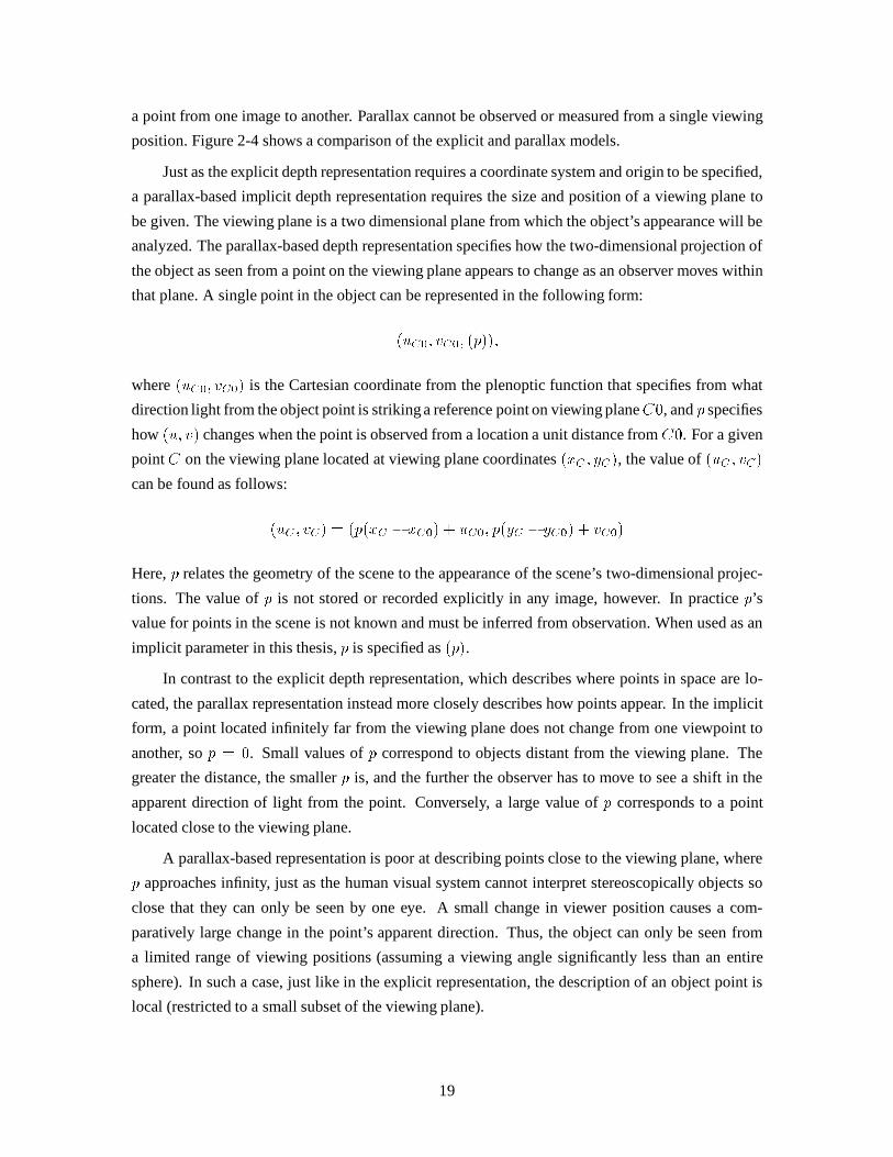
a point from one image to another. Parallax cannot be observed or measured from a single viewing
position. Figure 2-4 shows a comparison of the explicit and parallax models.
Just as the explicit depth representation requires a coordinate system and origin to be specified,
a parallax-based implicit depth representation requires the size and position of a viewing plane to
be given. The viewing plane is a two dimensional plane from which the object’s appearance will be
analyzed. The parallax-based depth representation specifies how the two-dimensional projection of
the object as seen from a point on the viewing plane appears to change as an observer moves within
that plane. A single point in the object can be represented in the following form:
(uC0; vC0; (p));
where(uC0; vC0) is the Cartesian coordinate from the plenoptic function that specifies from what
direction light from the object point is strikinga reference point on viewing planeC0, andp specifies
how(u; v) changes when the point is observed from a location a unit distance fromC0. For a given
pointC on the viewing plane located at viewing plane coordinates(xC ; yC), the value of(uC ; vC)
can be found as follows:
(uC ; vC) = (p(xC � xC0) + uC0; p(yC � yC0) + vC0)
Here,p relates the geometry of the scene to the appearance of the scene’s two-dimensional projec-
tions. The value ofp is not stored or recorded explicitly in any image, however. In practicep’s
value for points in the scene is not known and must be inferred from observation. When used as an
implicit parameter in this thesis,p is specified as(p).
In contrast to the explicit depth representation, which describes where points in space are lo-
cated, the parallax representation instead more closely describes how points appear. In the implicit
form, a point located infinitely far from the viewing plane does not change from one viewpoint to
another, sop = 0. Small values ofp correspond to objects distant from the viewing plane. The
greater the distance, the smallerp is, and the further the observer has to move to see a shift in the
apparent direction of light from the point. Conversely, a large value ofp corresponds to a point
located close to the viewing plane.
A parallax-based representation is poor at describing points close to the viewing plane, where
p approaches infinity, just as the human visual system cannot interpret stereoscopically objects so
close that they can only be seen by one eye. A small change in viewer position causes a com-
paratively large change in the point’s apparent direction. Thus, the object can only be seen from
a limited range of viewing positions (assuming a viewing angle significantly less than an entire
sphere). In such a case, just like in the explicit representation, the description of an object point is
local (restricted to a small subset of the viewing plane).
19

(x, y, z)
(xC0, yC0)(xC, yC)
(uC0, vC0)(uC, vC)
uC = p (xC - xC0) + uC0
vC = p (yC - yC0) + vC0
(uC0, vC0, (p))
Explicit depthrepresentation:each object pointhas three-dimensionalcoordinates
Parallax-basedimplicit depthrepresentation:object details movefrom viewpoint to viewpoint as given by
object point
camera plane
p is measure of parallax, animplicit parameter manifested in the observed change ofdirection between viewpoints
C0C
Figure 2-4: Explicit geometric and implicit parallax-based image representations of an object point.The geometric representation of a point is its three-dimensional location in space. The parallax-based representation of the same point describes how the point appears from the viewing zone.(uC0; vC0) is the plenoptic function’s description of the direction from which light from the pointstrikesC0, while the implicit parameter(p) is manifested by a change in this direction resultingfrom viewer motion fromC0 to a new pointC.
20

For other points located further from the viewing plane, a parallax-based representation is much
less local. A point’s representation is made up of information from all the viewing locations that
can observe it. A single point relatively far from the viewing plane can be seen from a wide range
of viewing positions; its effect is widely distributed. On the other hand, information about the point
is still coherent: the appearance of a point as seen from one viewer location is a good estimate
of the point’s appearance as seen from a proximate observation point. Furthermore, the implicit
parallax parameter assures that the direction of the light from the point not only changes slowly, but
predictably.
2.2.1 Directional emitters
So far, this discussion has included only descriptions of isolated points in space emitting light of
a particular color. These sources appear like stars glowing in space, never taking on a different
brightness or hue no matter how or from where they are viewed. This illumination model of om-
nidirectional emission is adequate to describe emissive and diffuse materials. Many natural objects
are made up of materials that have an appearance that changes when they are viewed from different
directions. This class of materials includes objects that have a shiny or specular surface or a micro-
scopic structure. Single, ideal points of such a material are calleddirectional emitters: they appear
to emit directionally-varying light. This definition includes points on surfaces that reflect, refract,
or transmit light from other sources; the emission of these points is dependent on their surrounding
environment.
To model a directional emitter using an explicit depth representation requires that extra in-
formation be added to the model to describe the point’s irradiance function. The light emitted by
each point must be parameterized by the two additional dimensions of direction. Since a direction-
by-direction parameterization would for many applications be unnecessarily detailed and expensive
to compute and store, this function is usually approximated by a smaller number of parameters.
The Phong light model of specular surfaces [57] is probably the most common approximation of
directional emitters.
In a parallax-based representation, the position of the viewer with respect to the object, and
thus the viewing direction, is already parameterized as part of the model. Incorporating directional
emitters into the parallax-based model is therefore easier than using the explicit depth model. A
directional emitter can be described completely if the emitter’s appearance is known from all view-
points. Alternatively, a lighting model can be used to approximately describe how the point’s color
changes when the surface it is located on is viewed from different directions. The parallax-based
representation already provides a framework for the linear change in direction of light that results
from viewer motion; the modeling of a changing color as a function of the same parameter fits this
framework.
21

2.2.2 Occlusion and hidden surfaces
Some object and shading models can be approximated as a collection of glowing points in space.
These kinds of models have been used for wire frame models for applications such as air traf-
fic control. Wire frame models and illuminated outlines are not, however, very applicable to the
recording, representation or display of natural objects. An accurate representation of real world
scenes must include some modeling of solid and occluding objects. Similarly, photorealistic image
display requires the ability to render opaque objects and, consequently, the occlusion of one object
by another.
The parallax-based implicit depth model is superior to the explicit depth model for represent-
ing scene occlusion. Recall that the parallax-based depth model is viewer-centric, while the explicit
depth model is object-centric. Occlusion is a viewer-centric property: whether or not a point oc-
cludes another is determined by the viewpoint from which the pair of points is viewed. The explicit
model is not associated with a viewer, nor is a point represented by this model associated with any
other point in the object. No way exists to define the visibility of a particular object point without
information about the rest of the object’s structure and the location of the viewer. The explicit model
is poor for representing occlusion specifically because its representation of object points is compact
and local: no model information exists on how other parts of the object effect light radiated from
the point.
The parallax-based model does not indicate what light is emitted from a particular point; rather
it specifies what light is seen from a given direction. Whether light traveling along a single line of
sight is the result of the contribution of a single point or the combination of transmitted, reflected,
and refracted light from many different points, the parallax model encodes the result as a single
direction. In the case where the object is composed of materials that are completely opaque (no
transparent or translucent materials), the parallax model records only the light from the point on
the object closest to the viewer lying along a particular direction vector. Many computer graphics
algorithms, such as the depth-buffer hidden surface algorithm, are effective in producing informa-
tion about the closest visible parts of objects; parallax-based models are good matches to these
algorithms.
2.2.3 Transparency
The window analogy
Transparent and translucent materials can also be described using the parallax-based method, but at
the expense of greater effort and computational expense. Imagine a clear glass window looking out
onto a outdoor scene. The relationship of the light from the scene and the window’s glass can be
thought of in two ways. Most commonly, perhaps, the glass seems like an almost insignificant final
22

step as it passes from the scene to the viewer’s eye. In this case, from a computational perspective,
the glass is almost a “no-op” when acting on the plenoptic function: an operation performed with
no resulting action. In computer graphics, the glass could be modeled as a compositing step where
the scene is the back layer and the glass forms an almost transparent overlay. When considered in
this way, the window appears most incidental to the imaging process.
Another way to consider the relationship between the window and the scene places the glass in
a much more important role. Light emerging from the scene streams towards the glass from many
different directions and at many different intensities. The back surface of the glass intercepts this
light, and by photoelectric interaction relays it through the thickness of the glass and re-radiates it
from the window’s front surface. An ideal window changes neither the direction nor the intensity
of the light during the process of absorption, transport, and radiation. The window is a complex
physical system with the net effect of analyzing the plenoptic function in one location and repro-
ducing it exactly in another. In this consideration of the window and the scene, the viewer is not
seeing the scene through an extraneous layer; instead, the viewer sees a glowing, radiating glass
pane that is interpreting information it observes from its back surface. From what object or through
what process this information comes to the glass is irrelevant to the viewer: only the glass need be
considered.
Parallax-based transparency
Non-opaque materials can be described in the parallax-based representation using this second model
of imaging. The visible parts of the object form a hull of visibility through which all other parts
of the object much be observed. Computational methods can be used to calculate the influence
of interior or partially occluded parts of objects on the light emitted from unoccluded parts of the
object. The rendering equation is a description of how energy is transported from each piece of
a scene to all others [39]. If the contribution of the energy from the otherwise invisible parts of
the object to the visible parts has been taken into account, the invisible parts need no longer be
considered. In fact, one of the main premises of image based rendering [46] states that the hull of
the object can be much simpler than its visible parts: it can instead be a more regular shape such
as a sphere, a polyhedron, or even a simple plane like the window pane. Exactly which type of
radiating hull is used and what method of finding the composite radiation profile of points on that
hull is implemented depends on the application and the types of scenes, objects, and materials to be
represented.
Geometry-based transparency and occlusion
The explicit depth model can also be adapted to include occlusion, but the process is more complex
than that for the equivalent parallax-based model. Direction emitters must first be implemented.
23
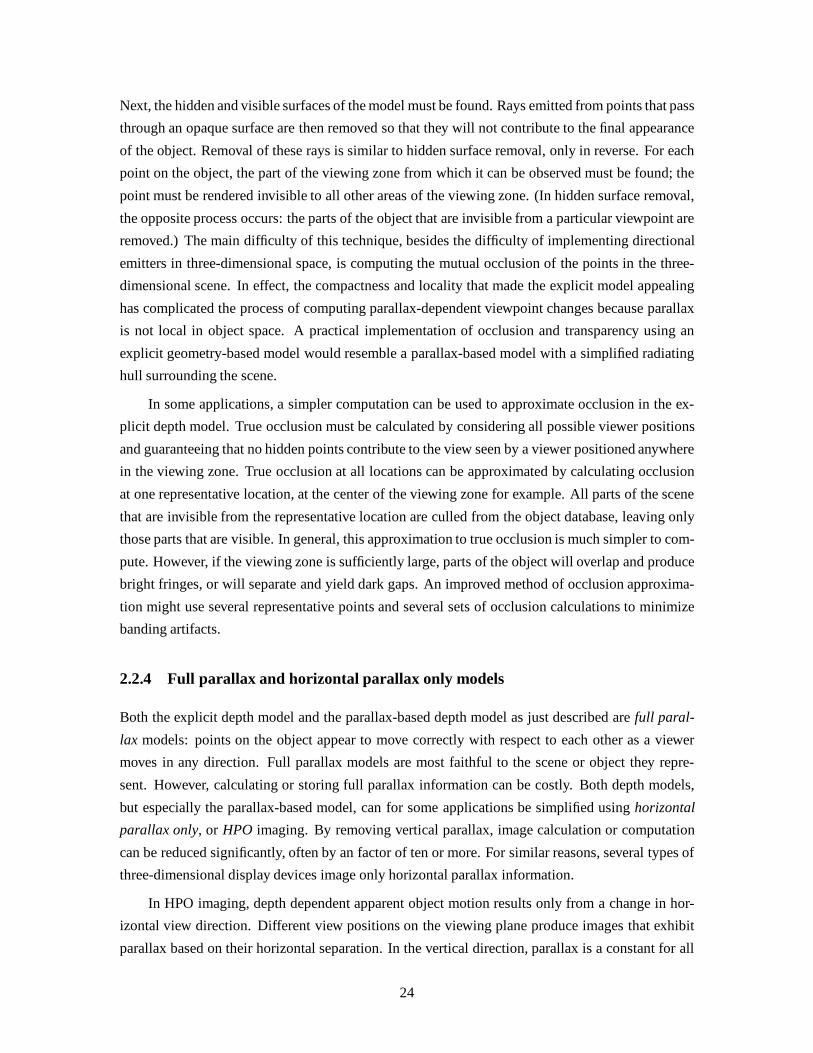
Next, the hidden and visible surfaces of the model must be found. Rays emitted from points that pass
through an opaque surface are then removed so that they will not contribute to the final appearance
of the object. Removal of these rays is similar to hidden surface removal, only in reverse. For each
point on the object, the part of the viewing zone from which it can be observed must be found; the
point must be rendered invisible to all other areas of the viewing zone. (In hidden surface removal,
the opposite process occurs: the parts of the object that are invisible from a particular viewpoint are
removed.) The main difficulty of this technique, besides the difficulty of implementing directional
emitters in three-dimensional space, is computing the mutual occlusion of the points in the three-
dimensional scene. In effect, the compactness and locality that made the explicit model appealing
has complicated the process of computing parallax-dependent viewpoint changes because parallax
is not local in object space. A practical implementation of occlusion and transparency using an
explicit geometry-based model would resemble a parallax-based model with a simplified radiating
hull surrounding the scene.
In some applications, a simpler computation can be used to approximate occlusion in the ex-
plicit depth model. True occlusion must be calculated by considering all possible viewer positions
and guaranteeing that no hidden points contribute to the view seen by a viewer positioned anywhere
in the viewing zone. True occlusion at all locations can be approximated by calculating occlusion
at one representative location, at the center of the viewing zone for example. All parts of the scene
that are invisible from the representative location are culled from the object database, leaving only
those parts that are visible. In general, this approximation to true occlusion is much simpler to com-
pute. However, if the viewing zone is sufficiently large, parts of the object will overlap and produce
bright fringes, or will separate and yield dark gaps. An improved method of occlusion approxima-
tion might use several representative points and several sets of occlusion calculations to minimize
banding artifacts.
2.2.4 Full parallax and horizontal parallax only models
Both the explicit depth model and the parallax-based depth model as just described arefull paral-
lax models: points on the object appear to move correctly with respect to each other as a viewer
moves in any direction. Full parallax models are most faithful to the scene or object they repre-
sent. However, calculating or storing full parallax information can be costly. Both depth models,
but especially the parallax-based model, can for some applications be simplified usinghorizontal
parallax only, or HPO imaging. By removing vertical parallax, image calculation or computation
can be reduced significantly, often by an factor of ten or more. For similar reasons, several types of
three-dimensional display devices image only horizontal parallax information.
In HPO imaging, depth dependent apparent object motion results only from a change in hor-
izontal view direction. Different view positions on the viewing plane produce images that exhibit
parallax based on their horizontal separation. In the vertical direction, parallax is a constant for all
24

points, as if the depth of all points on the object were identical. Given this constant vertical depth, a
constant parallaxPH can be calculated and used to find the direction of light from any view point:
(uC ; vC) = (p(xC � xC0) + uC0; PH(yC � yC0) + vC0)
HPO is an effective approximation because humans and most other organisms perceive depth
using horizontally-offset eyes or sensors. HPO provides stereoscopic depth to these systems. Hu-
mans can also move their eyes more easily from side to side than up and down, so many viewers of
HPO displays see horizontal image parallax without noticing that the vertical parallax is missing.
Applications that require great accuracy or image quality, however, should use full parallax imaging
when possible to maximize image realism.
The choice between the explicit depth model and the parallax-based implicit depth model de-
pends on the type of scenes or spatial information being represented, the method of scene data
acquisition and display, the desired speed of image computation, and theaccuracy of the final im-
age. The explicit depth model is a compact and local representation of object points, while the
parallax-based model is a less local representation of an object’s appearance as seen from a viewing
zone. For photorealistic image representation, the parallax-based model is generally more useful
because directional emitters and occlusion are simpler to implement.
The next section discusses imaging models and display devices capable of displaying depth.
Since the emphasis of this text is on photorealistic imaging, the parallax-based model and the de-
vices and image techniques that use it will be examined almost exclusively at the expense of the
explicit depth model.
2.3 Cameras and the plenoptic function
Besides the eye, a camera is the most common instrument used to measure the plenoptic func-
tion. The simplest camera, called a pinhole camera because its aperture is very small, analyzes the
plenoptic function at a single point. The point of analysis corresponds to the location of the aperture.
During the stages of the imaging process, light from the object can be parameterized in several
different ways, depending on the location from which the light is being observed. As previously
described, the light that appears to be radiated by a point of an object may actually be made up of
light contributed by many different parts of the scene. Each three-dimensional object point in its
environment has a characteristic function of radiation described by the plenoptic function measured
at the point. If a point radiates light towards the camera aperture, and no other point lies between
the point and the aperture, that point will be imaged by the camera onto the film. Most light emitted
by the object is not captured by the camera because it is either radiated away from the aperture or is
blocked by some other part of the object.
25

object points:(xO, yO, zO),each emitting light with
a function PO(θO, φO, λ).
camera location: (xC, yC, zC),intercepts light with a
function PC(uC, vC, λ).
object
film plane: Directionalinformation is encoded spatially in 2D as an image:
FI (X(uC), Y(vC), Λ),where X and Y are scalingfunctions.
3D spatialinformation
2D directional information
2D spatialinformation
Figure 2-5: A pinhole camera analyzes the plenoptic function of a three-dimensional scene.
26

object
Multiple cameras encode the object's depth information implicitly as the first derivative of image position (parallax).
Figure 2-6: Several cameras can be used to record depth information about a scene by sampling theplenoptic function at different locations.
While the structure of the object is three-dimensional and spatial, the camera records the struc-
ture as two-dimensional and directional by sampling the object’s light from a single location. The
direction of the rays passing through the pinhole is re-encoded as a spatial intensity function at the
camera’s film plane. Figure 2-5 charts the course of this conversion process. The pattern on the film
is a two-dimensional map of the plenoptic function as seen by the camera aperture. The intensity
pattern formed is a two-dimensional projection of the object; all depth information has been lost
(except for that information implicitly conveyed by occlusion and other monocular depth cues).
2.4 Parallax-based depth systems
A pinhole camera, then, is by itself unable to record depth information about a scene. Several such
cameras can, however, be used as part of a depth-sensitive instrument by sampling a scene’s plenop-
tic function from different locations. Figure 2-6 shows a multiple viewpoint camera arrangement.
27

free space(no occlusion)
camera plane
film plane
arbitrarilycomplex scene
Figure 2-7: Parallax-based imaging systems sample the direction of light at many spatial locations.
Since the image from each camera is a two-dimensional function, any three-dimensional in-
formation about the scene must clearly be encoded implicitly in the image data, not explicitly as
a depth coordinate. Implicit depth of an object point is recorded on the camera film by the dis-
tance the image of the object point moves as seen from one camera’s viewpoint to the next. This
image-to-image jump is called parallax. In a continuous mathematical form, parallax becomes the
first derivative in spatio-perspective space. All multiple viewpoint imaging systems, those using
multiple cameras to capture three-dimensional data about a scene, use this first-derivative encoding
to record that data onto a two-dimensional medium. Human vision is a good example of this type
of imaging system. We refer to this class of devices as parallax-based depth systems.
2.4.1 Parallax is three-dimensional information
Parallax-based imaging systems capture disparity information about a scene and produce an output
that to some approximation mimics the three-dimensional appearance of that scene. By sampling
the plenoptic function at a sufficiently high number of suitably positionedanalysis points, a parallax-
based imaging system can present a field of light that appears three-dimensional not just to a viewer
located at the viewing zone, but at any other view location as well.
28

discretizedvirtual imageof object
imagemodulation
projectors
view zone
Figure 2-8: If tiny projectors radiate the captured light, the plenoptic function of the display is anapproximation to that of the original scene when seen by an observer.
29

Figures 2-7 and 2-8 illustrate this process, which is exactly what the window pane in the pre-
vious example does to light from its scene. If the direction of light from an arbitrary collection of
sources can be sampled at many spatial locations, the visible three-dimensional structure of those
sources is captured. Furthermore, if tiny projectors (directional emitters) send out light from the
same points in the same directions, the appearance of that light will be indistinguishable from that
from the original scene. The mimicry is not just true at the point of analysis; the display looks
like the objects from any depth so long as no occluder enters the space between the viewer and the
display.
2.4.2 Display issues
Image display systems depend on the fact that a display device can mimic the recorded appearance
of a scene. A photograph, for instance, displays the same spatial pattern as recorded on the film of
the camera, and an observer interprets that image as a rendition of the scene. For this imitation to
be interpreted as a recognizable image by a human observer, the light emitted by the display must
have a certain fidelity to the light from the original object. In other words, the display approximates
the plenoptic function of the original scene. This approximation of the display need not be exact.
The required level of approximation required depends on the application of the display system.
For example, a black and white television image is coarsely sampled spatially and devoid of color
information; however, the gross form, intensity, and motion information it conveys is adequate for
many tasks.
The overwhelming majority of imaging and display systems present a plenoptic approximation
that contains neither parallax nor explicit depth information. Such systems rely on monocular depth
cues such as occlusion, perspective, shading, context, anda priori knowledge of object size to
convey depth information. These two-dimensional display systems usually also rely on the fact that
a human observer is very flexible in interpreting changes in scale from object to display. As a result,
a photograph of a person need not be enlarged to exactly the size of that person’s face in order to be
recognized.
This thesis is most concerned with devices that are capable of displaying recorded three-
dimensional information about scenes. Unlike two-dimensional displays, three-dimensional dis-
plays mimic an object’s plenoptic function by emitting directionally-varying light. The broad class
of three-dimensional displays can be divided into two smaller categories: volumetric displays,
which emit light from a range of three-dimensional points in a volume, and parallax displays, which
emit spatially-varying directional light from a surface. These two categories of output devices are
directly analogous to explicit and implicit depth recording methods.
30
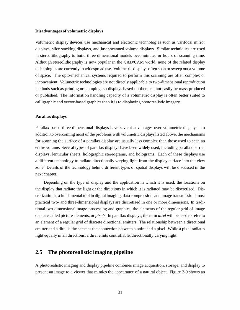
Disadvantages of volumetric displays
Volumetric display devices use mechanical and electronic technologies such as varifocal mirror
displays, slice stacking displays, and laser-scanned volume displays. Similar techniques are used
in stereolithography to build three-dimensional models over minutes or hours of scanning time.
Although stereolithography is now popular in the CAD/CAM world, none of the related display
technologies are currently in widespread use. Volumetric displays often span or sweep out a volume
of space. The opto-mechanical systems required to perform this scanning are often complex or
inconvenient. Volumetric technologies are not directly applicable to two-dimensional reproduction
methods such as printing or stamping, so displays based on them cannot easily be mass-produced
or published. The information handling capacity of a volumetric display is often better suited to
calligraphic and vector-based graphics than it is to displaying photorealistic imagery.
Parallax displays
Parallax-based three-dimensional displays have several advantages over volumetric displays. In
addition to overcoming most of the problems with volumetric displays listed above, the mechanisms
for scanning the surface of a parallax display are usually less complex than those used to scan an
entire volume. Several types of parallax displays have been widely used, including parallax barrier
displays, lenticular sheets, holographic stereograms, and holograms. Each of these displays use
a different technology to radiate directionally varying light from the display surface into the view
zone. Details of the technology behind different types of spatial displays will be discussed in the
next chapter.
Depending on the type of display and the application in which it is used, the locations on
the display that radiate the light or the directions in which it is radiated may be discretized. Dis-
cretization is a fundamental tool in digital imaging, data compression, and image transmission; most
practical two- and three-dimensional displays are discretized in one or more dimensions. In tradi-
tional two-dimensional image processing and graphics, the elements of the regular grid of image
data are called picture elements, orpixels. In parallax displays, the termdirel will be used to refer to
an element of a regular grid of discrete directional emitters. The relationship between a directional
emitter and a direl is the same as the connection between a point and a pixel. While a pixel radiates
light equally in all directions, a direl emits controllable, directionally varying light.
2.5 The photorealistic imaging pipeline
A photorealistic imaging and display pipeline combines image acquisition, storage, and display to
present an image to a viewer that mimics the appearance of a natural object. Figure 2-9 shows an
31

displayrenderingreadout/decoding
encoding/recording
storage
scenedescription
viewer
image
scene generation
Figure 2-9: A photorealistic imaging and display pipeline consists of many steps that transform acomputer graphic scene into visual data that the viewer interprets as a three-dimensional image ofthat scene.
example of a complete imaging pipeline. For synthetic images, rendering is just one of the steps
in the display of photorealistic computer graphics. Rendering transforms a scene description into
image information that can be encoded and stored in a recording medium or transmitted over a
channel. At the other end of the display pipeline, image data is read or received, decoded, and
displayed for a viewer.
The most straightforward way of approaching the rendering process, then, is to think of it as
the display process in reverse. For a parallax display, information can be rendered for a display by
computing the intersection of all rays leaving the display that pass through the object’s image and
intersect the viewing zone. In other words, the rendering process computes the synthetic plenoptic
function of the object throughout the viewing zone. This information can be computed in any order
and by any method; the encoding process that follows rendering is responsible for reformatting this
information into a display-compatible form.
If the ubiquitous computer graphics pinhole camera model is considered in the context of the
plenoptic function, each pixel of such a camera’s image is a measurement of the plenoptic function
along a unique ray direction that passes through the camera viewpoint. In order to sample the
plenoptic function over the entire surface of the viewing zone, a pinhole camera can be moved
to many different locations, capturing one viewpoint after another. To improve the efficiency of
the imaging process, acquisition can be simplified by spacing the camera at uniform locations, by
maintaining a consistent camera geometry, and by capturing no more view information than can be
used by a particular display device. These steps are optimizations, however; a sufficiently dense
and complete sampling of the plenoptic function throughout the viewing zone provides enough
information for any subsequent display encoding.
32

The next chapter develops the relationship between parallax display technologies and the com-
puter graphics rendering process that provides image information for them. It first describes the
general characteristics and technology of several parallax display types. Although these displays
depend on optics that vary from simple slits to lenses to complex diffractive patterns, they can be
related by a unified model precisely because they are parallax-based. This common display model
corresponds to a computer graphics model for image rendering. An understanding of both the ren-
dering and display ends of the imaging pipeline provides insight into the structure of the information
that must be produced for spatial display.
33
Chapter 3
Spatial display technology
The history of three-dimensional display devices includes many different technologies, several of
which have been repeatedly re-invented. Confusion in and about the field of three-dimensional
imaging is in part a result of the lack of a unifying framework of ideas that tie together different
display technologies. The recent increased interest in three-dimensional display technologies for
synthetic and dynamic display adds to the importance of providing this framework. This chapter
reviews the mechanics of the most prevalent parallax displays types, then builds a common parallax
display model that describes their shared properties. The camera geometry designed to produce
images for this common model serves as a basis for the computer graphics algorithms detailed in
this thesis.
3.1 Spatial displays
3.1.1 Terminology of spatial displays
Throughout its history, three-dimensional imaging has been plagued by poorly defined terminology.
Some of the most important terms in the field have definitions so overloaded with multiple meanings
that even experienced professionals in the field can often not engage in conversation without a
clarification of terms. Several of these terms are important in this thesis.Three-dimensional display
andspatial displayare used interchangeably to describe the broad category of devices that image a
three-dimensional volume. In particular, “three-dimensional images” should not be confused with
the two-dimensional projections of three-dimensional scenes that computer graphics produces. The
termautostereoscopicrefers to a device that does not require the viewer to wear glasses, goggles,
helmets, or other viewing aids to see a three-dimensional image.
A spatial display mimics the plenoptic function of the light from a physical object. The accu-
racy to which this mimicry is carried out is a direct result of the technology behind the spatial display
34

device. The greater the amount and accuracy of the view information presented to the viewer by the
display, the more the display appears like a physical object. On the other hand, greater amounts of
information also result in more complicated displays and higher data transmission and processing
costs.
As described at the end of the previous chapter, spatial displays fall into two different major
subclasses: volumetric displays and projectional or parallax displays. Volumetric displays image
points inside a volume, while parallax displays emit directionally varying light from a surface.
Parallax displays, because they are compatible with photo-realistic computer graphics images, are
described in detail in the next section.
3.1.2 Photographs: minimal spatial displays
A photograph can be considered a minimal spatial display. A photograph is a spatial representation
of the directional component of the plenoptic function as analyzed by a camera at one position
in space. This recorded information is played back in the familiar photographic form where this
single viewpoint is dispersed in all directions approximately equally. Since only one perspective of
the scene is recorded, the displayed perspective remains constant, independent of ultimate viewer
location. The photograph is capable, however, of recording single-view depth cues, thus conveying
an understandable spatial rendition of many objects.
3.1.3 Stereoscopes
Stereoscopes were the earliest optical devices developed to present more than one viewpoint of
an object to a viewer. The stereoscope developed by Wheatstone in 1838 was fundamental to his
seminal explanation of binocular depth perception. The development of stereoscopes by Brewster,
Holmes, and others led to a widespread popularity of three-dimensional photographs in Europe
and America in the late 1800’s. Viewers of similar optical design can still be seen today as View-
MasterTM toy viewers.
A stereoscope is the simplest spatial display that can image the directional component of the
plenoptic function at more than one position, thus providing disparity-based depth information to
an observer. A stereoscopic camera photographically samples the plenoptic function from two posi-
tions separated by a distance corresponding to the interoccular distance of a typical human observer.
A stereoscope displays these two photographs through separate optical channels in a way that min-
imizes crosstalk between the two images. The observer, when presented with the image pair, sees
the two disparate images and perceives stereoscopic depth.
While the stereoscope is a simple, elegant, and effective device, viewing images using it is
an inconvenient and solitary experience. An external optical device must be used to see the three-
dimensional image, and that image is visible to only one viewer at a time. A range of other tech-
35

nologies based on the same principles as the stereoscope have been used to present the two views
in a more convenient and accessible way. Several of these technologies permit a single stereoscopic
image to be viewed by several people at once. Multi-viewer displays use different multiplexing
techniques to encode both images onto a single screen, print, or piece of film. Examples of mul-
tiplexing mechanisms includes polarization (polarized projection or vectographs viewed through
polarized glasses), color (anaglyphic projection or printing using red and green or blue inks), or
temporal switching (motorized shutter disks or shutter glasses that block one of two sequentially
displayed images). Anaglyphic and polarized projection methods lend themselves to the display of
stereoscopic movies using the same display principles.
The geometry and construction of the stereoscope restricts the location of the viewer to essen-
tially one position. Although the other two-view display methods can relax this constraint, a moving
viewer is still presented with the same two camera viewpoints. Since true three-dimensional objects
change in appearance when a viewer moves, such a stationary three-dimensional display fails in
its mimicry of reality. The paradox of an unchanging image in the face of egomotion is mentally
reconciled with the false conclusion that the displayed object is in fact constantly moving to always
present the same face to the viewer. This illusion of motion both distracts the viewer and provides
no additional information about the object’s three-dimensional structure.
More advanced versions of the stereoscope solve this problem by tracking the physical location
of the observer and capturing or computing the two images that the observer’s eyes should see. In
these systems, observer motion is reflected in a natural change in displayed viewpoint. In other
words, the viewer’s location is used to determine where to sample the plenoptic function of the
scene. In addition to eliminating the image tracking illusion, these types of parallax displays can
be very effective because they permit the viewer to experience not just stereoscopic depth, but
also motion parallax. Motion parallax, the apparent motion of the scene that occurs in response to
egomotion, is a strong depth cue for many types of scenes. For synthetic image display, observer-
tracking systems are computationally very demanding. Two new viewpoints must be rendered at
irregular locations at high enough frame rate and low enough latency to keep up with a motion
of a viewer. Systems that fail to maintain this rate can produce a disorientation called “simulator
sickness”.
3.2 Multiple viewpoint display technologies
Motion parallax can be displayed without the need for continuous tracking, acquisition and display
of two viewpoints by using a display device that constantly displays several different viewpoints of
the objects to appropriate locations in the view zone. These projected location in space are known as
virtual view apertures. As the viewer’s eye falls into the aperture corresponding to a viewpoint, the
appropriate view information becomes visible on the display. Binocular depth can be conveyed if
36

slit aperture
image data
view information
opaque barrier
illumination source
Figure 3-1: A parallax panoramagram display consists of slits in an opaque parallax barrier.
the viewer’s two eyes fall into two different apertures. These multi-view displays inherently contain
more image information than do their two-view counterparts. The extra view information about a
scene that the display requires must be captured or computed in some way. The mechanism of the
display device or the complexity of the electronics used to drive it is usually more complicated than
that used in two-view systems.
3.2.1 Parallax barrier displays
Parallax barrier displays are among of the earliest autostereoscopic display technologies. Displays
of this type consist of a series of regularly spaced, narrow slits in an opaque barrier material (Fig-
ure 3-1). These slits are positioned above an imaging medium such as a piece of high resolution
photographic film. The display is brightly back lit so that stripes of the film are visible through the
slits of the display. The separation between the slits and the film permit different parts of the film to
be visible when the display is viewed from different directions.
Two types of three-dimensional displays use parallax barriers. The first developed, theparallax
stereogram, was developed by Fredrick Ives in 1903 [37]. Under each slit of the parallax stereogram
are two long vertical strips of image information, one from a left eye view and the other from the
right. From a small range of viewpoints, an observer looking through the slits of the display see one
view with one eye and the other view with the other eye. The purpose of the barrier is to prevent
the viewer’s eye from seeing the other eye’s view information. The image data for all slits of the
parallax stereogram is created by interleaving columns of the left and right view images.
37

Between 1918 and 1928, Kanolt [40] and Fredrick’s son Herbert Ives [38] independently ex-
tended the parallax stereogram to display more than two views. This new display was called a
parallax panoramagram. Instead of two interleaved views behind each slit, the parallax panoram-
agram uses a vertical column from each of a series of horizontally-varying views to form a slit’s
image. The barrier must block out all but one of these views from an observer, so the ratio of slit
thickness to barrier width is smaller in the parallax panoramagram than in the parallax stereogram.
The parallax panoramagram displays horizontal directional information in the same way that a
pinhole camera stores a scene onto film. Each location on the imaging medium behind a slit lies on
a line of unique slope passing through the slit. Light passing through the imaging medium from the
backlight forms a fan of rays radiating from the slit. All points on the surface of the display other
than those lying on a slit can radiate nothing at all; the spatial component of the display’s plenoptic
function is inherently point sampled at the slit locations. To the viewer, the samples appear as bright
lines of the scene overlaid by black stripes. Point sampling thus produces image artifacts because
some points of the object being imaged cannot be seen from some or all directions.
Depending on the method by which a parallax panoramagram is recorded, the directional in-
formation encoded by each slit may be a continuous function or a collection of discrete samples.
Discrete versions are more commonplace. For example, the underlying image medium may be
composed of discrete picture elements, or the image information used to make the parallax panora-
magram may come from a collection of pinhole cameras located in fixed positions. A continuous
version could be recorded using either a camera with a slit aperture moving on a track, or a fixed
camera with a set of cylindrical lenses. Whether discrete or continuous, the exact means of record-
ing the directional information significantly affects the appearance of the final image.
3.2.2 Lenticular sheet displays
The parallax barrier’s major shortcoming is its low optical efficiency. Only a small amount of light
can pass through the narrow slits from the light source and image behind. The rest is absorbed by
the barrier. The larger the number of views recorded behind each slit, the less light that can pass
through the increasingly small slit openings. (Smaller slits also lead to loss of image resolution due
to diffraction from the slit edges.) Large parallax barrier displays require banks of lights behind
them to achieve sufficient brightness.
An alternative to the parallax panoramagram’s “pinhole camera” approach to imaging is the
“lenticular sheet” display, which uses cylindrical lenses instead of slits to display the image medium
(Figure 3-2). More properly, this type of display is called alenticular panoramagram, but it is more
often just called alenticular. In a lenticular panoramagram, each lens focuses light from a range
of horizontal positions on the imaging medium and directs all of it out towards theviewing zone,
the distance at which the viewer will be located. Unlike a parallax barrier display, a lenticular sheet
absorbs very little light during display.
38

cylindricallenslet
image data
view information
Figure 3-2: A lenticular panoramagram is an HPO display using long, cylindrical lenses.
Lenticular panoramagrams have higher image quality compared to parallax panoramagrams.
Assuming that the lenticules are positioned to focus the film plane to the viewing zone, small ranges
of image data will appear to fill the entire lenticule horizontally. The image data is effectively
replicated across the width of the lenticule. Only the small gaps between lenticules will have no
image information at all.
Both lenticular and parallax panoramagrams are prone to crosstalk between the information for
adjacent lenticules or slits. Usually, nothing separates the image data associated with one slit from
the data for the slit next to it. From extreme viewpoints the information from one slit or lens can be
viewed through its neighbor. The effect on the entire image can be one of either a sudden perspective
change or a depth inversion. This problem can be reduced by placing informationless black “guard
bands” in between the image data for adjacent elements. Both types of panoramagrams also suffer
from the fact that the simultaneous spatial encoding of multiple perspective views in the imaging
medium considerably reduces the horizontal spatial resolution of the final display. This encoding
also limits the amount of view information that can be stored.
3.2.3 Integral photography
The integral photograph [47] [20] or integram is very similar to the lenticular sheet display except
that it images the directional component of the plenoptic function as a two-dimensional, rather than
one-dimensional, function (Figure 3-3). Integral photographs are thus capable of full parallax dis-
play. Some early integral photographs were made from pinhole sheets, but the optical efficiency
of the result was so poor as to render them impractical. Instead, a sheet of spherical or “fly’s eye”
lenses are used to project image information from an array of two-dimensional images located be-
39

sphericallenslet
image data
Figure 3-3: An integral photograph, or integram, uses spherical lenses to display both horizontaland vertical parallax.
hind them. Compared to lenticular panoramagrams, storing the two-dimensional directional image
information for each lenslet in a spatial encoding is even more costly than storing just the horizontal
dimension. Integral photographs sacrifice significant spatial resolution in both dimensions to gain
full parallax.
3.2.4 Holography
The hologram was first invented by Gabor in 1948 [25], and applied to image display by Leith and
Upatnieks [44]. Functionally, a hologram behaves much like an integral photograph with extremely
small lenses. Light from an illumination source is diffracted in different directions by a contin-
uous range of sites on the hologram’s surface. As a result, holograms are capable of producing
three-dimensional images of a spatial quality andaccuracy unparalleled by other technologies. The
continuity of the wavefront radiated by a hologram can coherently focus the image of object de-
tail. Thus, just like a volumetric display, a holographic image can provide the human depth cue of
accommodation.
Holograms store directional information about the plenoptic function differently than do other
types of parallax displays. Holograms encode directional information as interference fringes of
varying spatial frequency. The scale of these fringes can range from about 100 to about 5000
line pairs per millimeter for display holograms. When the fringes of a hologram are illuminated
appropriately, they diffract light that recreates the object’s plenoptic function. The high information
density of the holographic medium is directly responsible for the fidelity of the holographic image.
40

Ironically, the hologram’s huge information storage capacity is also one of the medium’s chief
disadvantages: the high information density demands careful physical processes and intensive com-
putational techniques in order to create the holographic pattern. If the diffraction pattern is optically
encoded, recording the fine structure of the interference fringes requires high resolution, insensitive
recording materials and vibration-isolated exposure apparatus. The phase sensitivity of holography
dictates that a coherent optical source such as a laser must be used. Direct computation of fringe
patterns instead of optical exposure is currently possible only for the crudest images because of the
large amount of image data required. Although the hologram is a remarkable device, most of its
practical uses involve some form of information reduction.
3.2.5 Holographic stereograms
The holographic stereogram is a holographic display type with significantly reduced information
requirements. Many of the characteristics of lenticular and parallax panoramagrams also apply to
holographic stereograms. Indeed, as Okoshi has noted [56], the holographic stereogram should
more correctly be called a holographic panoramagram to reinforce this familial connection. Instead
of the hologram’s continuous representation, the holographic stereogram uses discrete sampling
and interpolation to reduce the amount of image information both spatially and directionally. The
image data is usually stored in the recording medium either optically or electrically. Holographic
stereograms of the type considered here are an outgrowth of work by DeBitetto in 1969 [18].
The mechanical and optical simplicity of the holographic stereogram, in conjunction with the
information capacity of the underlying holographic material, permits a wide range of possible trade-
offs between quantity of image data, image fidelity, and ease of manufacture. Most holographic
stereograms are usually horizontal parallax only and display approximately 50 to 1000 discrete
view directions at every spatial location on the display surface. These stereograms are made using
a master-transfer, or “two-step”, process. Other holographic stereograms can be recorded directly
on the output media in a single step; these “one-step” stereograms are usually HPO and discretize
spatial position rather than direction. Full parallax displays can be created in either one-step or
two-step form. The flexibility of the holographic stereogram to span the range between the simple
photograph to the complex hologram is mitigated by difficulties of illumination and the wavelength
dependencies of diffractive optics.
3.3 A common model for parallax displays
The basic behavior of a large class of multi-view three-dimensional displays, including parallax and
lenticular panoramagrams, integral photographs, and holographic stereograms, can be described
using the disparity-based depth model. In each of these displays, spatial locations on the display
surface act as directional emitters for the disparity information that the display presents. The most
41

important differences between the various displays are whether the spatial or directional encodings
are continuous or discretized, the type of interpolation of the displayed information, the optical
coherence of the light leaving the display, and the presence or absence of vertical parallax. These
characteristics are determined by the recording, storage and output imaging technologies used in
the display. McCrickerd contributed early insight into the similarities of these displays [50].
Since these displays are parallax based, each encodes depth implicitly as image information.
The image data that parallax displays require can be acquired by cameras arranged in arrays or
moving on tracks. These displays can also use image information produced using computer graph-
ics algorithms that compute the appearance of a virtual scene as seen from specific locations or
viewpoints. The quality of the final image produced by the display is a function of the input data,
the encoding of the directional information contained in it, and the characteristics of the display
device itself.
Another common characteristic of this display class is that most such devices image the scene
using only horizontal parallax. The direls used in HPO display devices accurately approximate the
directional component of the plenoptic function only in the horizontal direction. Such display ele-
ments appear different when viewed from varying horizontal positions, but maintain an appearance
of constant intensity when seen from different vertical positions. An HPO display has a fixed verti-
cal depth for all parts of the scene. Typically, the constant depth is set so that scene details appear
to have a vertical location at the plane of the display. HPO is a common engineering tradeoff in
the fabrication of parallax displays. The information bandwidth of HPO displays is usually sig-
nificantly less than for full-parallax displays, so the image recording and display mechanisms for
these displays can be simpler. HPO displays may use the saved bandwidth to provide higher spatial
resolution.
Figure 3-4 shows the relationship between a full-parallax parallax display and its viewing zone.
In this case, the viewing zone is discretized into apertures: each direl of the display sends a ray
bundle of a given intensity towards each aperture. An observer in the view zone intercepts this light
from the direl as well with light emitted from other direls in different directions that intersect the
same view aperture. The display appears to be a single image made up of these different directional
components. Each view aperture is a place in the viewing zone where the plenoptic function of the
display closely corresponds to that of the object being imaged.
Similarly, Figure 3-5 shows an HPO parallax display and its view zone. Here, the viewing zone
is broken into long thin vertical apertures, with the intensity of light leaving the display’s direls re-
maining constant over the vertical span of each aperture. The HPO display can have fewer apertures
than the full-parallax version, so less information needs to be captured, stored, and displayed.
All planar parallax displays can be approximated using a model based on these diagrams. A
common model of disparity-based displays allows imaging and computational methods to be cre-
ated for the entire class of displays, rather than for one particular type. The differences between the
42

display
viewing zone
outputaperture
direl
full parallax
Figure 3-4: A discrete, full-parallax parallax display and the two-dimensionalgrid of view aperturesthat it projects.
43

viewing zone
outputaperture
direl
horizontal parallax only
display
Figure 3-5: An HPO parallax display projects a one-dimensional grid of long, thin view apertures.
44

physics of the different disparity-based displays are relatively minor compared to the strong simi-
larities in their display geometries, information content, and sampling issues. The general model
of parallax displays is sufficiently detailed to match the display to the other stages of imaging (im-
age acquisition or synthesis, data recording and storage, data retrieval) without introducing image
artifacts or distortions. During display analysis and design, display-specific characteristics can be
included once the fundamentals of the general model have been addressed.
3.4 Implications for image generation
At the time when most disparity-based displays were developed, the required image data was cap-
tured from natural three-dimensional scenes using an array of cameras, a moving camera on a track
or grid, or a specialized optical device. The advent of computer graphics has led to the need for
three-dimensional displays of virtual scenes, and an increasing number of commercially-made par-
allax displays are now authored and rendered using computers. Most image generation techniques
are tailored to specific devices without consideration of more general models and principles. The
growing demand for synthetic three-dimensional displays foreshadows the need for more efficient
ways to generate images for them. The common model of parallax displays provides a foundation
upon which computer graphics image generation techniques can be built.
Capturing or generating image information for parallax displays consists of calculating the
appearance of each direl as seen from each view aperture. Thedisplayand view planes of the
viewing geometry correspond to theimageandcameraplane in the recording or rendering geometry.
Every view aperture located at the view plane has a corresponding camera position on the camera
plane. Ray bundles sent from each direl to each view aperture correspond to lines of sight from each
camera to the image plane. A synthetic camera’s lines of sight are pixels in the camera’s image.
Figure 3-6 demonstrates the camera geometry that corresponds to the parallax display shown in
Figure 3-4. Figure 3-7 is the camera geometry used to capture images for the HPO parallax display
shown in Figure 3-5.
Undistorted spatial images require a direct correspondence between image generation and dis-
play geometries. Given this constraint, the camera model can be used to estimate the amount of
image data required to produce a parallax display. For full parallax imaging for a display withm�n
direls ands � t view apertures,s � t cameras must render images with at leastm � n pixels of
raw image data each. An HPO display withs view apertures will requires camera views. Indepen-
dent of the method of image generation, spatial displays of a given construction and fidelity require
this amount of raw rasterized image data for display. The image generation requirements for even
simple multi-view parallax displays is much higher than for the same resolution two-dimensional
image.
45

image plane
camera plane
camera location
object
full parallax
Figure 3-6: A full-parallax camera geometry used to capture images for the the common parallaxdisplay model. This arrangement of cameras corresponds to the PRS camera geometry described inChapter 5.
Since the amount of raw image information is fixed by the characteristics of the display, rapid
generation of image data must rely on efficient image generation techniques rather than information
reduction. As the next chapter will show, however, traditional computer graphics algorithms are
relatively inefficient when generating images of complex synthetic scenes.
46

image plane
camera plane
camera location
object
horizontal parallax only
Figure 3-7: The camera geometry for horizontal parallax only displays. This camera geometry isreferred to in Chapter 5 as the LRS camera geometry.
47

Chapter 4
Limitations of conventional rendering
If existing algorithms were sufficiently fast or otherwise well suited to the task of synthesizing im-
ages for parallax displays, there would be little practical need to explore more specialized rendering
methods specially designed for that purpose. Each perspective of the image sequence could be
rendered by a computer graphics camera, one at a time, using optimized general-purpose graphics
software and hardware. The simplicity and economy of this approach would be quite alluring.
Unfortunately, the current state of computer graphics software and hardware is insufficiently
powerful to compute perspective images at a high enough frame or data rate to support high quality
dynamic three-dimensional displays. The high information density of multiple viewpoint displays
assures that the process of image generation will remain challenging at least for the forseeable
future. This section demonstrates inefficiencies in existing computer graphics techniques, and how
the properties of perspective image sequences can be used to increase the efficency of rendering.
4.1 Bottlenecks in rendering
The complexity of object descriptions in computer graphics has continued to increase to match the
maturity of rendering algorithm design, the performance of computer processors, and the size of
computer memory available. Most scanline computer graphics algorithms were originally devel-
oped in the 1970’s. At that time, most object descriptions were coarse, devoid of the level of detail
found in scene descriptions today. Such objects can be represented by a relatively small number of
vertices, with each geometric primitive of the object spanning a relatively large number of pixels in
the final raster or display device. The ratio of the number of pixels shaded in the final raster to the
number vertices in the object description represents a trade-off between the relative costs of pixel
and vertex operations. For reference in this text, we will refer to the pixel-to-vertex ratio as�.
In most computer graphics systems, vertex operations are comparatively expensive when com-
pared to pixel fill operations. Vertices are usually floating point coordinates, while pixels are often
48

integer or fixed point values. Vertices are manipulated individually with relatively costly matrix
operations, while pixels can be drawn in spans or warped in parallel. Vertices are also typically sent
across the general purpose bus that connects the computer system’s CPU to its graphics hardware,
whereas pixel information more often flows over much higher speed internal bus, into memory, and
out to a display subsystem.
If the � of an object description closely matches a graphics system’s optimal�, the time re-
quired to render the object will be minimized. On the other hand, if an object has a much higher�
than that for which the graphics system is optimized, the rendering process will be limited by the
maximum speed that primitives can be converted to pixels. Conversely, an object with too low a�
for a particular architecture will be limited by vertex-related factors.
In order to meet the requirement of interactive image display and manipulation, early graphics
subsystems were designed to efficiently render objects of low vertex count, minimizing expensive
vertex operations and relying on image coherence to accelerate rendering. In other words, the
hardware was optimized to render scenes of high�. As time passed, geometric databases became
more complex and detailed to match the increasing sophistication of computer hardware as well
as the multi-fold drop in the price of computer memory. Higher object detail translates directly to
smaller polygons and a larger number of vertices. During the same time, the number of addressable
pixels of output devices (and thus the number of pixels an algorithm needs to render) has also
increased, but physical limitations of display devices have restricted the rate of this growth to a
factor of about four to six. Computer graphics hardware has adapted to rendering these higher
fidelity databases by reducing the target�, increasing the amount and speed of the hardware dealing
with per-vertex calculations.
Without algorithmic changes, however, matching the� of scene descriptions and the optimal
� of graphics hardware has become increasingly difficult. Many highly detailed databases are ap-
proaching the point that triangle primitives have shrunken to approximately the size of a pixel (a
� of approximately1=3). While such small geometry remains useful for surface interpolation and
antialiasing, the hardware required to perform so many per-vertex operations and to transmit the
vertex information have a prohibitively high cost. Large geometric databases are also expensive in
terms of external storage and I/O.
4.2 Improving graphics performance
Several approaches have been used to reduce the optimal� in current graphics architectures and
algorithms. One of the simplest ways is to usevertex sharingto minimize the redundancy of a
vertex data set. Vertex sharing is a class of techniques based on the assumption that most objects
are not composed of a set of individual polygons, but instead of surfaces made up of adjacent
ones. Adjacent surface polygons share vertices. By describing the surface not as a list of polygons
49

but as a collection of triangle or quadrilateral strips, meshes, or fans, the number of vertices can
be significantly reduced. A triangle strip, for example, describes a set of adjacent triangles with
approximately one vertex per triangle for long strips. Thus, about three times as many triangles
can be described with the same number of vertices using sufficiently long triangle strips. Some
geometry-building algorithms are amenable to outputting triangle strips or meshes, while others are
not, so the practically of vertex sharing depends on the kind of objects most likely to be used.
Similarly, some of the communications costs associated with a large number of vertices can
be reduced by compressing the vertex data before transmission across the graphics bus, and de-
compressing it before rendering [19]. Such compression schemes rely on the coherence that exists
between vertices that are close together and surface orientation vectors that are closely aligned.
The positions of two vertices adjacent in a data stream, or better yet those of three vertices that
represent an object triangle, are likely to be statistically correlated and representable by a smaller
number of bits than if each vertex is considered alone. Deering claims typical compression rates of
approximately 6 to 10, including the gains made by triangle sharing.
Another option to reduce� is to use higher order geometric functions such as spline patches to
represent surfaces of objects. For many objects these more expressive primitives can significantly
reduce the size of the object’s geometric description. The description is sent across the system bus to
the graphics subsystem, where it is almost always converted into polygonal primitives. In this way,
the system bus becomes less of a bottleneck in the rendering process, although vertex hardware is
still required to deal with the internal polygonal primitives. Unfortunately, many types of geometric
data are not amenable to representation with higher-order primitives.
A different approach to improving rendering efficiency is to replace geometric detail with im-
age detail using texture mapping. A texture map consists of raster data that can be stored in the
graphics subsystem, warped, and drawn onto scene geometry. The scale of the geometry no longer
needs to be on the scale of the smallest image detail. Rather than decreasing the optimal� for a
graphics system, texture mapping permits objects of high� to have much greater image detail.
Texture mapping has successfully been implemented in all but the least costly graphics archi-
tectures. Textures, however, are most effective for data reduction when the objects in the scene are
mapped with repetitive patterns so that texture images can be reused; otherwise, the cost of tex-
ture memory and texture data transfer can quickly become high. Texture maps can also not replace
highly complex geometry or smooth polygonal silhouette edges. Most texture map algorithms are
view independent: they appear the same when viewed from any direction. Related but more compli-
cated texture map algorithms such as bump mapping [9] and view dependent textures [17] add view
dependent shading parameters. These algorithms are currently seldom implemented in hardware.
50
4.3 Testing existing graphics systems
The following two experiments show the relative vertex and pixel-fill limits that define� for a range
of computer graphics rendering systems. Both experiments were performed on three machines: a
Silicon Graphics Indigo R4000 with an Elan graphics subsystem; a Silicon Graphics Indigo2 R4400
with a Maximum Impact; and a two processor Silicon Graphics Onyx R4400 with a RealityEngine2
graphics engine. These three machines span a range of performance from entry workstations to high
end rendering engines. In both experiments, a set of equally-sized isosceles triangles were drawn
to the screen using the OpenGLTM graphics library [11]. Each triangle was described by three
independent vertices consisting of three-dimensional location, color, and a normalized direction
vector. The color of each vertex was determined solely by the vertex color which was interpolated
by across the triangle by the graphics hardware; the direction vector was not used for lighting
purposes.
The first experiment measures the amount of time required to render a fixed number of triangles
of a given area. A scene of 10,000 triangles was repeatedly rendered into a 256 pixel wide by 256
high pixel RGB window. The total rendering time was divided by the number of polygons drawn
to find the rendering time per polygon. This time, in microseconds per polygon, is plotted against
polygon area in Figure 4-1.
Independent of graphics platform, each curve shows an initial flat line for small polygons,
followed by a linearly increasing line for progressively larger polygons. The flat part of the line
shows that for small polygons, the cost of processing the 30,000 vertices per scene dominates the
cost of filling the resulting pixels. (Since both vertex and pixel operations occur in parallel, only the
greater of the two is reflected in the total rendering time.) Beyond a certain point, linear increases
in area are directly reflected as linear increases in rendering time.
Figure 4-2 shows the result of a related but slightly different experiment. This test measures
the total time to draw 500,000 pixels into an800 � 800 pixel RGB window using triangles of a
given size. This total time corresponds to rendering an object that has been tesselated into varying
numbers of triangles, but spans the same size on the screen. When large triangles are used, the
rendering time is almost independent of polygon size, and the lines are flat. In this region, pixel
filling dominates the rendering time. Below a certain area, the cost of the larger number of vertices
dominates the fill costs, resulting in longer rendering times. These renderings are vertex limited.
To be sure, the optimal� for a given machine or scene is dependent on a number of factors not
measured in these experiments. Polygon shading, orientation, aspect ratio, screen alignment, and
pixel processing could all affect rendering performance and change�. These tests do show, though,
that for typical rendering operations and polygons, graphics subsystems of a wide range of power
are each optimized for a� corresponding to triangles ranging from about16� 16 to about50� 50
51

0 500 1000 1500 2000triangle area (pixels)
0
5
10
15
20m
icro
seco
nds/
tria
ngle
pixel fill rate limits10,000 triangle scene
Indigo ElanIndigo2 Mx ImpactOnyx RE2
256
512
892
Figure 4-1: Results of an experiment designed to test the pixel fill rate behavior of three differentgraphics architectures. The experiment consisted of filling 10,000 identical triangles using OpenGL.Different runs of the experiment used triangles of different sizes.
pixels. Objects tesselated with polygons about the size of single pixels may take up to two orders
of magnitude longer to render than objects made up of polygons of this optimal size.
In summary, the� of geometric scene descriptions has decreased steadily over time with de-
velopment of computer hardware. Traditional computer graphics algorithms and hardware exploit
the image coherence most prevalent in scene descriptions of high�. These mechanisms are less
efficient when rendering the complex, detailed scene descriptions that have become more common
in recent years. Such objects typically have fewer large, featureless patches that can be represented
by large polygons. Moreover, many objects have inherent geometric complexity — it is unlikely
that efficient geometric descriptions will soon emerge that can efficiently encode them. Image co-
herence continues to play a smaller and smaller role in high quality computer graphics. Other forms
of coherence must be used in order to more efficiently represent geometry to graphics hardware and
software and to turn it into pixels.
52

101
102
103
104
105
triangle area (pixels)
100
101
102
103
draw
tim
e (m
illis
econ
ds)
vertex limits500,000 pixels filled
Indigo ElanIndigo2 Mx ImpactOnyx RE2
175
490
645
Figure 4-2: Experimental results of a vertex performance test. 500,000 pixels were drawn on thescreen using different numbers of triangles.
4.4 Using perspective coherence
As we have seen previously, a characteristic of parallax-based systems as compared to explicit ge-
ometric models is that object information is not compact or local: information about small parts
of an object is distributed over a wide range of image information. This important characteristic
is an useful guide in helping to overcome the “� barrier” when rendering multi-perspective im-
ages. In traditional computer graphics, the three-dimensional geometric model is projected onto
a two-dimensional plane to form an image. If the geometry is expressed in an explicit three-
dimensional form, the two-dimensional projection of the data will share the local property of the
three-dimensional model. Three-dimensional vertices are projected into two dimensions, forming
geometric primitives that can be scan converted. If the scene geometry is complex, however, the
footprint of the each scene polygon is a small area with a position and shape that must be recom-
puted when each perspective image is rendered.
53

Alternatively, the multi-perspective rendering process can be altered to fit more naturally the
characteristics of the parallax-based images. Rather than using the spatial coherence of the scene to
simplify the rendering process, the coherence between the appearance of the scene from one view-
point to another can instead be exploited. This inter-viewpoint, or perspective, coherence provides
a way to convert scene geometry into larger rendering primitives while still permitting interpola-
tion and other incremental techniques to be used to improve the performance of scan conversion,
shading, and hidden surface removal.
Perspective coherence is one type of scene coherence that is resistant to increases in object
complexity. Perspective coherence depends on the fact that scenes appear similar when viewed
from proximate camera positions. The location and shade of visible objects in a scene tends to
remain constant or vary slowly with respect to varying viewpoint. Furthermore, objects that are
visible from one viewpoint are also likely to be visible from a range of similar viewpoints. Our
real world experience supports these claims: most objects in our surround do not flash or become
quickly visible and invisible as we change the direction from which we gaze upon them. In this
way, perspective coherence is more often valid and dependable for complicated scenes than is image
coherence.
The next chapter will examine the properties of image coherence in spatio-perspective space,
and will describe an algorithm designed to take advantage of it. This technique, called multiple
viewpoint rendering, can greatly increase� and therefore make the scene more efficient to render.
54

Chapter 5
Multiple viewpoint rendering
The previous chapter of this thesis demonstrated that single viewpoint rendering algorithms are
inefficient when the images they render have limited spatial coherence. Single viewpoint rendering
also does not use the perspective coherence that exists in abundance in image data recorded from
closely-spaced viewpoints. This chapter shows how the rendering process can be adapted to exploit
perspective coherence in order to efficiently sample the plenoptic function from multiple viewpoints.
5.1 The “regular shearing” geometry
We begin by considering more closely the camera geometry used for parallax displays as shown in
Figures 3-6 and 3-7. The capture cameras are arranged in a regularly-spaced linear or planar array
located at the camera plane. The orientation of each of the cameras is identical: each camera faces
so that its optical axis is perpendicular to the camera plane, and each camera’s plumb line or up
vector is aligned with the camera plane’s vertical axis. The lens of each camera can be shifted to
recenter the image plane in the camera view. An object located on the image plane will appear in
the same location in each camera’s image. Figure 5-1 details the camera orientation with respect to
the camera plane.
We will refer to the two-dimensional camera arrangement shown in Figure 3-6 as theplanar
regular shearing(PRS) camera geometry. A PRS camera captures full-parallax information about
a scene. Similarly, the one-dimensional array of cameras in Figure 3-7 is called thelinear regular
shearing(LRS) camera geometry, which captures only horizontal parallax information. When either
the one-dimensional or two-dimensional cases is appropriate, the general termregular shearing, or
RS, will be used. Since the scene is assumed to be static, the concept of a camera array is used
interchangeably with the idea of a single camera moving sequentially from one viewpoint to the
next.
55

y
x
all camera up vectors are parallel to camera plane y vector
all camera optical axesare perpendicular to camera plane
Figure 5-1: A closeup of the camera orientation used in the PRS camera geometry. The optical axisof each camera is perpendicular to the camera plane, while each camera’s up vector is aligned withthey axis of the camera plane.
As we have previously seen in Figure 2-4, the apparent direction of light from a single three-
dimensional point in a scene changes linearly in proportion to a change in viewpoint location when
an observer moves in a plane. In the RS geometry, the spacing of cameras is linear and is restricted
to the camera plane or track. Thus, a scene detail also appears to move linearly in the image of
one camera view to the next (assuming no occlusion of the detail occurs). The alignment of the
camera’s orientation with respect to the camera grid produces the result that a change in horizontal
camera viewpoint produces a strictly horizontal motion of scene detail. Similarly, a change in
vertical viewpoint produces a change in only the vertical position of scene detail in a PRS camera
arrangement. For simplicity, our initial emphasis here will be on HPO imaging. Later, the concepts
will be extended to include full parallax camera geometries. Figure 5-2 shows a two-dimensional,
“Flatland” [1] view of the RS camera geometry, where images of a two-dimensional scene are
captured by a camera moving along a horizontal track. Each camera images is a one-dimensional
projection of the scene onto a line of film.
In 1987, Bolles, Baker and Marimont used an LRS geometry in their work on image analysis
using many camera viewpoints [12]. These vision researchers were looking for structure in three-
dimensional scenes captured by many cameras. To simplify their algorithm, they usedepipolar
planesto limit the search for corresponding points in different images. An epipolar plane is the
plane that includes two or more camera locations and a point in the object. The location of the image
of the object point as seen from each viewpoint must lie along the line of intersection between the
epipolar plane and the image plane. This line is called anepipolar line. The “epipolar constraint”
effectively reduces the search for corresponding points from a two-dimensional matching problem
to a one-dimensional one. Their work also assumes that the scene is static, so that any image-to-
56

L R
optical axes
camera plane
image plane
object
Figure 5-2: A two-dimensional view of the PRS camera geometry.
image change is the result of camera motion. Bolleset. al.’s work also includes experiments with
other camera geometries and addresses issues of camera calibration. Here we depart from their
approach and concentrate on the properties of the spatio-perspective volume as produced by LRS
cameras, while using their terminology as appropriate.
5.2 The spatio-perspective volume
When an RS camera is used to capture an image of a scene, each camera viewpoint in the grid
produces a two-dimensional projection of the scene on its film plane. These two-dimensional im-
ages can be arranged by viewpoint location to form an image volume called thespatio-perspective
volume. For a PRS camera geometry, the spatio-perspective volume is four-dimensional, while the
simpler LRS geometry produces a three-dimensional volume. In the LRS case, the image volume
include all of the camera images stacked in front of each other with the rightmost view being in front.
The picture on the left in Figure 5-3 shows a spatio-perspective volume composed of a collection of
computer graphics images captured using an LRS camera geometry.
Two dimensions of this spatio-perspective volume include the horizontal (x) and vertical (y)
spatial dimensions of each camera image; the third dimension, perspective (p), is the camera loca-
tion. Although the volume of image data may be discretized spatially by the camera’s sensors and in
perspective by the individual viewpoints, the spatio-perspective volume spanned by the image data
is a continuous space.
57

L
R
L
Rspatio-perspective volume epipolar plane image
Figure 5-3: An spatio-perspective volume derived from a synthetic scene is shown on the left; on theright is an EPI from the volume. EPIs are horizontal slices through the volume, where perspectiveviews are vertical slices.
5.2.1 Epipolar plane images
The appearance of the perspective images that are the vertical planes of the spatio-perspective vol-
ume in Figure 5-3 is familiar. The volume itself, though, can be sliced along other axes to form
different images that do not correspond to single perspectives. For instance, Figure 5-3 shows a
horizontal plane being extracted from the spatio-perspective volume. This plane inx-p space is
composed of thenth horizontal scanline from each camera image in the image stack. Each one of
these scanlines lies along a common epipolar plane in the LRS camera geometry. Bolleset. al.
named this image of the slice through the spatio-perspective volume anepipolar plane image, or
EPI. The EPI is the image space in which the rendering algorithms described in this chapter will
draw.
The properties of the LRS camera geometry constrain scene details to move strictly horizon-
tally from view to view. Therefore, each EPI can be considered separately from all others because
no part of an object will appear in two different EPIs. Reducing the scene that is being imaged from
three to two dimensions as shown in Figure 5-2 in effect also reduces the spatio-perspective volume
to a single EPI. The following examples use this “Flatland” scene representation to better explain
the EPI’s properties.
Figure 5-4 shows a “Flatland” LRS camera imaging a simple scene consisting of three points.
The points are located behind, in front of, and at the image plane. The one-dimensional images
from the camera are assembled to form a two-dimensional epipolar plane image. Figure 5-5 shows
the EPI produced by the camera. Each line in the EPI is the track of the corresponding point in the
scene. At the viewpoint from where one point occludes another, the tracks of the points through the
EPI cross.
58

L R
Figure 5-4: A camera in an LRS geometry captures images of a three point scene.
L
R
x
p
Figure 5-5: The epipolar plane image of the three point scene.
59

The linear track representation of a three-dimensional point is one of several properties of the
epipolar plane image volume that makes it useful for image analysis. Algorithms for detecting linear
features in images are common. Since the search algorithm need only look within an EPI for data
from a single track, the search process is a two- and not three-dimensional one. Once the path of
a linear track through the volume is determined, the depth and position of the corresponding point
can be found given that the parameters of the capturing camera are known.
5.2.2 Polygons and polygon tracks
Most computer graphics scene databases consist of polygons instead of just points. Polygons are
graphics primitives that describe patches of surface. Most computer graphics algorithms and hard-
ware are optimized for polygon drawing, sometimes even more so than for line drawing. For a
three-dimensional scene, the vertices of polygons sweep out linear tracks through spatio-perspective
space. The area between the vertices is swept out by the surface of the polygon itself. The area of
the spatio-perspective volume swept out by a polygon is called apolygon track, or PT.
Figure 5-6 extends the scene in Figure 5-4 to include two “Flatland” polygons (lines) connect-
ing two pairs of the vertices. Figure 5-7 shows the spatio-perspective volume that corresponds to
the resulting two polygon scene. The large shaded areas are the PTs from the two polygons. The PT
from the front polygon occludes the PT from the more distant polygon. The PT of the rear polygon
crosses itself as the camera transitions from viewing the polygon’s front surface to viewing its rear
surface. Since the polygons in the scene have a solid color that is not dependent on view direction,
the PTs also have a constant unvarying color over their surface area.
5.2.3 Polygon slices and PSTs
A polygonal three-dimensional scene can be reduced to a set of lines like those shown in Figure 5-6
by intersecting the scene’s polygons with the each epipolar plane. Each polygon is decomposed into
a set of horizontalpolygon slicesthat lie along scanlines of the image sequence. Each polygon slice
sweeps out a region of its corresponding EPI called apolygon slice track, or PST. PSTs can also be
thought of as slices through a PT.
The exact shape of a PST depends on the orientation of its slice and its distance from the image
plane. Figure 5-8 shows several examples of polygon slice orientation and the corresponding PST
shape. For all shapes, the horizontal edges of a PST are the projection of the polygon slice onto
the image plane as seen from the far left and far right camera locations. These edges are called
projected edges, orp-edges. The non-horizontal edges of each PST are the tracks of the endpoints
of the polygon slice. These edges, called interpolated edges ori-edges, interpolate between the two
projections of the slice through all camera viewpoints.
60

L R
Figure 5-6: The three points of the scene are joined with two surfaces.
L
R
x
p
Figure 5-7: The EPI resulting from the new scene. Large areas are swept out by the surfaces.
61
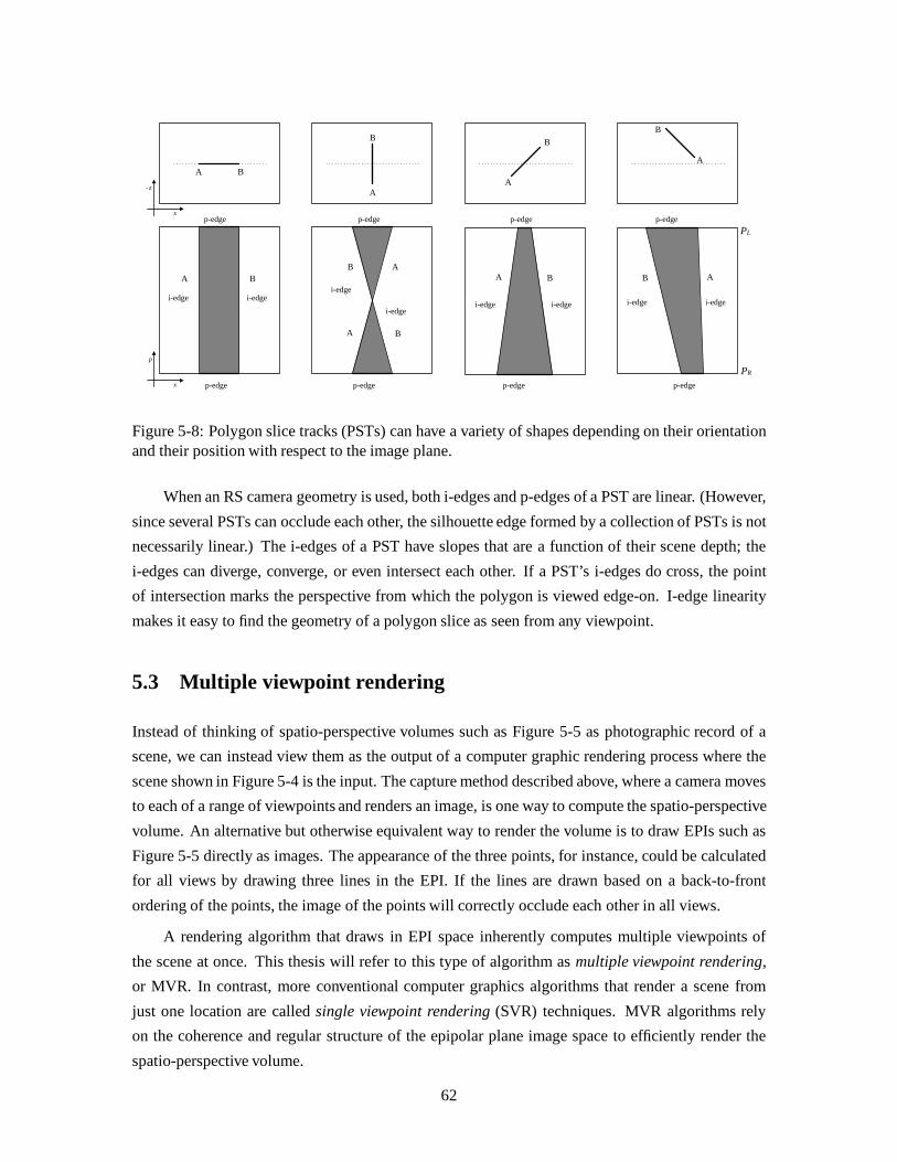
x
- z
x
p
PL
PR
p-edge p-edgep-edge
p-edge p-edgep-edgep-edge
p-edge
i-edge i-edgei-edge
i-edgei-edge i-edge i-edge i-edge
A B
A
B
A
B
A
B
A BAB
A B AB
A B
Figure 5-8: Polygon slice tracks (PSTs) can have a variety of shapes depending on their orientationand their position with respect to the image plane.
When an RS camera geometry is used, both i-edges and p-edges of a PST are linear. (However,
since several PSTs can occlude each other, the silhouette edge formed by a collection of PSTs is not
necessarily linear.) The i-edges of a PST have slopes that are a function of their scene depth; the
i-edges can diverge, converge, or even intersect each other. If a PST’s i-edges do cross, the point
of intersection marks the perspective from which the polygon is viewed edge-on. I-edge linearity
makes it easy to find the geometry of a polygon slice as seen from any viewpoint.
5.3 Multiple viewpoint rendering
Instead of thinking of spatio-perspective volumes such as Figure 5-5 as photographic record of a
scene, we can instead view them as the output of a computer graphic rendering process where the
scene shown in Figure 5-4 is the input. The capture method described above, where a camera moves
to each of a range of viewpoints and renders an image, is one way to compute the spatio-perspective
volume. An alternative but otherwise equivalent way to render the volume is to draw EPIs such as
Figure 5-5 directly as images. The appearance of the three points, for instance, could be calculated
for all views by drawing three lines in the EPI. If the lines are drawn based on a back-to-front
ordering of the points, the image of the points will correctly occlude each other in all views.
A rendering algorithm that draws in EPI space inherently computes multiple viewpoints of
the scene at once. This thesis will refer to this type of algorithm asmultiple viewpoint rendering,
or MVR. In contrast, more conventional computer graphics algorithms that render a scene from
just one location are calledsingle viewpoint rendering(SVR) techniques. MVR algorithms rely
on the coherence and regular structure of the epipolar plane image space to efficiently render the
spatio-perspective volume.
62

5.3.1 Basic graphical properties of the EPI
An image such as Figure 5-5 can be drawn efficiently using computer graphics techniques. A simple
line equation is a sufficient description to draw each track. The line’s slope is dependent on the depth
of the corresponding point, while the position of the line depends on where ineach view the point
appears. Recall that a point’s Cartesian description is compact (contains no redundant information)
and local (represents a small part of space). In comparison, the line description of the point’s track
is also compact, but the line itself is not local because it spans many perspectives.
The non-locality of the line description of a point track in EPI space translates into more effi-
cient rendering. EPI point tracks are linear features of the type for which scanline computer graphics
algorithms are often optimized. Rasterization of EPI tracks can be performed efficiently. Tracks are
long features that typically remain visible for large segments of image space, so the constant costs
associated with setup for rendering a line can be amortized over the many inexpensive incremental
calculations that occur when drawing the pixels along the line’s length. In short, The EPI space
brings together the images of the point from all views and incorporates them into a single geometric
primitive.
In order to explain the implications for rendering the spatio-perspective volumes of three-
dimensional scenes using MVR, we consider Figure 5-3 in more detail. The figure shows an EPI
extracted from an HPO spatio-perspective volume of a computer graphic scene. The scene consists
of three objects: a diffuse cube and star and a shiny cone. These objects were rendered using a
hardware-based polygon renderer that calculates the Phong light model at each polygon vertex and
uses Gouraud or linear shading to fill the interior pixels of the polygons. The selected EPI shown
on the right is made from image data near the middle of each image.
Figure 5-9 demonstrates some of the useful properties of the epipolar plane image space. The
EPI is made up of the image of many PSTs, but structure and coherence in the image are clearly
visible. Since a polygon slice that is visible from one viewpoint is usually visible from a range of
proximate viewpoints, the PSTs in the image are very long. The shading of the objects in the scene
are also fairly constant with respect to perspective. For diffuse objects such as the cube and star, the
color is independent of viewpoint, so the shade of those object’s PSTs changes only with horizontal
position and remains constant with respect to perspective. Large primitives with slowly varying
shading are very efficient for graphics algorithms to render.
For some non-diffuse objects such as the cone, color varies only slowly with respect to view-
point. The white streak on the cone’s track in the EPI is an approximation to an specular highlight
moving across the surface. Specular highlights are not attached to the surface upon which they
appear; for objects with high curvature the specular highlight can move rapidly across the surface
as the viewpoint changes. The cone was rendered using a Phong light model applied to each scene
vertex in each perspective view, so the specular highlight does not remain a constant shade.
63

L
R
vertices sweepout linear tracks
shading oftenconstant orslowly varying
simple back-face detectionand culling
large polygon-like primitives
occlusion
approximatedspecular highlight
Figure 5-9: EPIs have graphical properties that make them appealing to render.
Even though the EPI space is different from conventional image space, occlusion relations
between objects hold in the EPI just as they do in a perspective image. The image of the star, for
instance, is overlapped by the cube and the cone both in the original image sequence and in the EPI.
This depth relationship is important because it means that graphics primitives can be rendered into
EPIs using conventional hidden surface removal techniques.
These properties of epipolar plane images and PSTs can be harnessed by a multiple viewpoint
rendering algorithm to efficiently synthesize image information. A high-level diagram of an MVR
rendering process for an LRS camera geometry is shown in Figure 5-10. The input to the rendering
system is a geometric scene description. Transformation and lighting operations are performed
on the vertices of the geometry to compute the scene’s appearance as seen from extreme camera
viewpoints. Next, the geometry is intersected with the scanlines of the final image to form a set of
geometric slice primitives. These slices are stored in a table, sorted by scanline. Each entry of the
table is processed independently to render EPIs in the spatio-perspective volume. The slices of the
table entry are converted to PSTs. The PST is the fundamental rendering primitive of MVR: each
PST is rasterized in turn into its EPI. The spatio-perspective volume is complete after all EPIs have
been rendered.
The next section will present a more detailed overview of the MVR rendering process by re-
lating it to the conventional SVR rendering pipeline. The basic algorithm is followed by more in-
depth information about particular rendering techniques such as back-face culling, hidden surface
removal, view independent shading, texture mapping, and reflection mapping.
64

for each scanline
scene database
per-vertexcalculationsand polygonslicing
scanline slice table
slice to PSTconversion
EPI rasterization
Figure 5-10: A high-level block diagram showing the MVR system designed to render a spatio-perspective volume for an LRS camera geometry
5.4 The MVR algorithm
A typical SVR algorithm generates a perspective image sequence by reading in the model, trans-
forming it into world space, repeatedly transforming the scene geometry based on the position of a
moving camera, performing shading calculations, and scan converting the result to produce the final
image rasters. Although some operations such as view independent lighting could be performed
once for the entire image sequence, most implementations execute them once per view.
As a general rule, MVR reduces the cost of producing the perspective image sequence by
performing as many calculations as possible just once per sequence rather than once per view.
Model input, transformation, lighting, clipping, and scanline intersection all happen entirely or in
part during the initial startup process. The fewer remaining operations are done repeatedly aseach
EPI is rendered. By considering the image sequence as a whole, MVR reduces the cost of scene
synthesis.
Furthermore, MVR capitalizes on the increased coherence of the EPI to render primitives more
efficiently. Rendering PSTs, with long extent and often slowly-varying shading, is more efficient
than rendering a larger number of smaller polygons. PSTs also have a more regular shape and are
easier to rasterize than a general polygon. Increased rendering efficiency, combined with reduced
number of per-view operations, makes MVR faster than SVR for sufficiently long image sequences.
Figure 5-11 shows a comparison between the SVR and MVR rendering pipelines.
5.5 Overview
Figure 5-12 follows the MVR algorithm through the process of rendering a simple triangle
scene. The MVR algorithm differs from SVR beginning at the view transformation step: view
transformation is done once per image sequence, not once per view as in SVR. Instead of computing
65

model input
model transform
viewing transform
clipping
polygon rasterization
display
shading
model input
model transform
viewing transform
PST rasterization
display
horizontal clipping
vertical/depth clipping
scanline intersectionlighting
lighting
shading
once per EPI
once per view
once per sequence once per sequence
transformedpolygons
polygonslices
(x, y, z)
(x, y, z, w)
(xL, xR, y, z, w)
(x, y, z)
single viewpoint rendering multiple viewpoint rendering
perspective divide
perspective divide
Figure 5-11: The MVR pipeline compared with the more conventional SVR pipeline.
66

the transformed geometry from one camera location after another, the MVR algorithm performs
only the two transformations that correspond to two different camera viewpoints along the view
track. These two viewpoints are typically the most extreme camera locations along the view track;
if they are not, the coordinates from the extreme camera locations can readily be determined. Since
the camera moves in an LRS camera geometry, every scene vertex moves strictly horizontally and
linearly through positions indicated by these two transformations. Every scene vertex(x; y; z), then,
produces a transformed homogeneous coordinate(xL; xR; y; z; w) that specifies the vertex location
as seen from the extreme camera views:(xL; y; z; w) and(xR; y; z; w). The cost of performing the
combined transformation is less than the cost of two ordinary transformations because they, z, and
w coordinate values only need to be computed once.
After transformation, MVR performs an operation similar to scan conversion to slice the trans-
formed polygons into scanline-high primitives. Conventional scan conversion uses an edge table or
similar data structure to find the boundaries of scanlines by interpolating between polygon vertices.
MVR uses the same method to find the intersection of each polygon with each scanline. While
scan conversion rasterizes the interpolated spans into pixels, MVR’s slice conversion produces a
collection of polygon slices that are in three-dimensional space and continuous. Each slice has two
endpoints:(xL; xR; y; z; w)0 and(xL; xR; y; z; w)1. Note thaty0 = y1 because the two endpoints
by definition lie on the same scanline. Slices that fall above or below the view volume can be
clipped and discarded because no translation of the shearing camera can cause them to move into
view. Similarly, near and far plane depth clipping can also be done at this point.
Once slice conversion has reduced the entire scene into polygon slices, the slices are rendered
into the EPI volume. The volume is rendered EPI by EPI, with each EPI rendered separately by con-
verting the polygon slices that intersect it into PSTs. The conversion from a polygon slice to a PST
is relatively simple. The four vertices of a PST are as follows:(x0L; PL; z0; w0), (x1L; PL; z1; w1),
(x0R; PR; z0; w0), and(x1R; PR; z1; w1), wherePL andPR are the minimum and maximum per-
spective coordinate values in spatio-perspective space.
The PSTs that are rendered into an EPI are clipped, culled, shaded, and rasterized using tech-
niques much like those of conventional scan conversion. In some cases, properties of the PST
L
R
}
x
y
z x
p
zx
y
zx
y
z
Transformed polygon scene geometry (xL, xR, y, z, w).
Polygon is intersected with the scanlines of the screen.
Polygon slices are formed by interpolating between vertices.
Each slice is converted to a PST and rendered into a different EPI.
Figure 5-12: The basic MVR rendering pipeline as applied to rendering a triangle.
67
simplify the process or rasterization and rendering. The details of the techniques of each of these
rendering steps will be discussed individually in the next section.
5.6 Specific stages of MVR
5.6.1 Geometric scan conversion
The process of scan conversion, as the name implies, converts geometric primitives into scanlines
of the image raster. SVR scanline algorithms convert polygons that have been projected onto the
view plane into pixels of the final image. The particular implementation of the rendering algorithm
used may restrict the geometry of the input polygons in order to simplify rendering. For instance,
all polygons might have to be convex, or have only three vertices. Further restriction on the shape of
polygons is not practical even when characteristics may significantly affect performance. Polygons
may be very large or very small, have tall or wide aspect rations, or have edges or vertices that are
not aligned with the scanlines of the image.
Most scan conversion algorithms use a data structure such as an edge table to traverse the
edges of a polygon, finding endpoints of horizontal scanlines. The geometric parameters assigned
to the vertices of the polygon are linearly interpolated along the polygon edges to find values for
the endpoints of the horizontal spans. Once all the spans have been found, the endpoint values are
further interpolated to find the values for each pixel lying along the span. The simplest polygon, the
triangle, usually requires horizontal interpolation between two pairs of opposing edges to fill all the
scanlines.
In MVR, the polygon slicing process performs the scanline intersection function of SVR scan
conversion. MVR’s actual scan conversion is the process of converting the geometric description of
a PST into the pixels of an EPI. Compared to an arbitrary polygon, a PST is geometrically simpler
and graphically easier to render. Assuming a polygon slice remains within the camera’s field of
view throughout all viewpoints and that no other clipping or culling occurs, both p-edges of the
corresponding PST are screen aligned to the top and bottom scanlines of the EPI. Under the same
restrictions, both i-edges span all scanlines of the EPI.
Interpolation of geometric parameters is also easier when rendering a PST than when rendering
an arbitrary polygon. Figure 5-13 explains how the parameters of the PST are interpolated. When
the polygon slice is formed, the slice’s two endpoints are interpolated from the positions of the
polygon vertices. The constanty coordinate of the two endpoints is used for assigning the polygon
slice to an EPI but is otherwise not used during scan conversion. When rendering the PST, thex
coordinate values of the two slice endpoints are interpolated along i-edges between the extreme left
and right perspectives. Thez andw coordinate values remain fixed along i-edges since the depth of
a vertex remains constant with perspective under the RS camera geometry.
68

1dp
(x0L, PL, z0, w0)
(x0R, PR, z0, w0)
(x1L, PL, z1, w1)
(x1R, PR, z1, w1)
PL
PR
1
ds
(x1s, ps, z1, w1)(x0s, ps, z0, w0) (xp, ps, zp, wp)
x0s = ds x0R + (1 - ds) x0L
x1s = ds x1R + (1 - ds) x1L
xp = dp x1s + (1 - dp) x0s
zp = dp z1s + (1 - dp) z0s
wp = dp w1s + (1 - dp) w0s
p-edge
p-edge
i-edgei-edge
ps = ds PR + (1 - ds) PL
Figure 5-13: Interpolation of geometric parameters is similar to, but simpler than, the process ofinterpolating across the surface of a polygon. The large black dots are the vertices of the PST. Thepositions of the PST vertices are determined based on the data stored in the corresponding polygonslice. The scanline endpoints indicated by the gray dots are found be linearly interpolating alongeach i-edge. The normalized interpolation parameterds varies from zero to one over the range of allscanlines. The value for each pixel along a horizontal scanline is found by linearly interpolating thescanline endpoint values using the parameterdp. A pixel sample is shown in the figure as a whitedot. In addition to the geometric parameters shown, the view independent color ofeach pixel canbe found by a similar interpolation process.
69

After the location of all points along each i-edge have been determined, the pixels in the interior
of the PST can be found by interpolating along horizontal lines between the two i-edges. Thex
coordinate value is an interpolation of the already-interpolatedx endpoint values, while thez and
w coordinate values will always vary linearly from the value of one endpoint to another. In the case
where i-edges intersect each other, the interpolation process will move step from the left to the right
i-edges for all perspectives on one side of the intersection point, and from right to left on the other
side.
5.6.2 View independent shading
Computer graphics often approximates the behavior of a class of diffuse, emissive, or constant
colored materials by assuming that the material’s appearance does not change when viewed from
different directions. A view independent model is very efficient to implement in MVR because
the color of a polygon slice is independent of perspective. As a direct result, the shading of the
corresponding PST does not vary in the perspective direction. The shading of a PST varies strictly
horizontally from i-edge to i-edge. If the shading operation is thought of as a color-computing
function, a view independent function is one-dimensional and only needs to be sampled at different
rates to produce all the scanlines of a PST.
Another type of light model assumes that polygons are sufficiently small and that the color of an
object varies slowly enough that lighting calculations can be performed just at the vertex locations
of the scene’s polygons, and not at every pixel. The view independent version of this model is
called Gouraud shading. The Gouraud shading algorithm performs per-vertex lighting calculations,
computes a single color value, and linearly interpolates the color across the polygon. The process of
interpolation is very similar to, and often performed at the same time as, the geometric interpolation
of scan conversion.
MVR can efficiently render Gouraud-shaded scenes by performing view independent lighting
calculations at the vertices of the scene polygons, interpolating those values first to find the color of
the endpoints of the polygon slices, then interpolating again to calculate each pixel of the scanline.
The color of a vertex is constant with respect to perspective, so the color of each i-edge is also a
constant. The interpolation of the color vector is exactly the same as the scalar interpolation of thez
orw geometric coordinate values. Figure 5-14 shows the shading of a self-intersecting PST. As the
figure demonstrates, each horizontal line of the PST is a simple resampling of an identical shading
function derived by linear interpolation of the two endpoint values.
5.6.3 Back face culling and two-sided lighting
Back face culling is the process of removing surfaces from the scene geometry that face away from
the camera in order to reduce the cost of rendering. Back face culling assumes that the shading
70

E0 E1
polygon slice
V1R
V1L
V0R
V0L
x
p
PL
PR
E1 = (x1L, x1R, y, z1, w1)E0 = (x0L, x0R, y, z0, w0)
V0R = (x0R, PR, z0, w0) V0L = (x0L, PL, z0, w0)
V1R = (x1R, PR, z1, w1) V1L = (x1L, PL, z1, w1) direction of shading interpolation
Figure 5-14: Interpolating view independent shading parameters uses the same mathematics asgeometric interpolation.
71

E0
E1
PL
PR
PT
vR
vT
x0Lx1L
x1Rx0R
dL = x1L - x0L
dR = x1R - x0R
dL - dR
dLvT = vR
x
p
if dLdR < 0
dL
dR
vR = PR - PL
vT = PT - PL
camera track
image plane
polygon slice
Figure 5-15: Back face culling and two-sided lighting operations can be inexpensively performedby using similar triangles to calculate the perspectivePT where the polygon is seen edge-on.
properties of a surface are valid for its front face only. For many objects, back facing surfaces are
often occluded by front facing ones, so omitting them has no effect on the final rendering of the
scene.
On the other hand, it is sometimes useful to use surfaces that can be seen from both the front
and back. For example, interior surfaces of mechanical models used in computer aided design
applications may have a different color so they are clearly visible in cutaway drawings. Bidirectional
surfaces can have other distinguishing material properties in addition to different colors for the front
and back face. Back face culling is not appropriate for two-sided surfaces. Instead, a two-sided
lighting model is used to perform separate lighting calculations depending on the orientation of the
surface.
In SVR, back face culling and two-sided polygon rendering techniques are implemented by
computing the dot product of a polygon’s surface normal with the camera’s eye vector. The sign of
the dot product specifies if the polygon is facing toward or away from the camera. The dot product
must be calculated for every polygon at every viewpoint.
In MVR, a simple geometric technique can be used to compute in which views a polygon slice
faces forward or away from the camera. Figure 5-15 shows the general principle applied to a single
polygon slice. The PRS camera geometry guarantees that only three possible conditions can occur
to a polygon slice’s relative direction through in image sequence: the slice is always front facing, it
72

is always back facing, or it transitions once from one orientation to the other. In the first two cases,
a single dot product of the eye vector with the polygon slice normal determines a slice’s orientation
through all views.
In the third case, the PST of the polygon slice can be divided into a front and a back facing
section by finding the point of transition between the two. This transition perspective is the point
where the PST’s i-edges intersect each other. From this viewpoint, the polygon slice is seen edge-
on and subtends no screen width. All perspectives to one side of the transition perspective face in
one direction; all those on the other side face the other way. Different rendering parameters can be
applied to the two pieces of the PST to implement two-sided lighting, or the back facing piece can
be culled. (In hardware implementations of MVR, breaking self-intersecting PSTs into two pieces
is recommended because most rendering hardware supports only convex rendering primitives.)
Whether or not a PST intersects itself, and the location of the transition perspectivePT if it
does, can be found using thex coordinates of the vertices of the PST. These coordinate values are
x0L; x0R; x1L; x1R. Let dL anddR be the signed widths of a PST’s p-edges:
dL = x1L � x0L
dR = x1R � x0R (5.1)
If dRdL < 0, then the PST crosses itself. The transition perspectivePT can be found using the ratio
of the two signed widths as detailed in Figure 5-15.
5.6.4 Hidden surface elimination
Hidden surface elimination or removal prevents surfaces occluded by other parts of an object being
visible in a rendered image. Hidden surface elimination in MVR can use most of the techniques
common in SVR. One of the simplest techniques for hidden surface elimination is depth buffering.
When a PST is scan converted into an EPI, the depth of every pixel of the PST’s image can be
interpolated from the depth values of the polygon slice’s endpoints. A image precision buffer holds
the depth of the frontmost primitive at every pixel in the EPI. A newly rendered pixel from a PST is
only written into the EPI if its pixel depth is closer to the camera than the pixel value already written
at that spatial location. An MVR depth buffer shares all the strengths and weaknesses of SVR depth
buffering.
Depth buffering is an example of animage spacerendering technique because it performs depth
comparisons based on pixels of the image and not on scene geometry. Algorithms that use scene
geometry instead of pixel-level primitives are calledobject spacetechniques. MVR can use other
hidden surface techniques, both image space and object space algorithms. Object space algorithms
are usually easier to implement in MVR than in SVR because of the simple two-dimensional geom-
etry of the epipolar plane filled with one dimensional polygon slices. In contrast, SVR algorithms
73

often split, sort, and re-order planar geometric primitives in three-dimensional space. Furthermore,
the number of polygons that intersect one particular scanline of an image is usually a small fraction
of the total number of polygons in a scene. MVR only has to process this subset, which decreases
the cost and increases the locality of geometric operations.
5.6.5 Anti-aliasing
Anti-aliasing techniques are used to eliminate or avoid aliasing artifacts due to image discretization.
Anti-aliasing in MVR is exactly analogous to that used in SVR. The process is somewhat different,
however, because the images being rendered are not viewpoints, but EPIs.
Anti-aliasing an EPI filters image detail in the spatial domain in one dimension and in per-
spective in the other. Spatial anti-aliasing is commonly used in computer graphics. Perspective
anti-aliasing, which are less common, can be used to guarantee that object detail seen from one
viewpoint will not jump to a non-overlapping spatial location in another. Perspective anti-aliasing is
important when information from different views will be combined either optically in an autostereo-
scopic display or computationally in an image based rendering system [31].
Spatial anti-aliasing in the EPI band limits only the horizontal detail of the image. Vertical
anti-aliasing must be done using data from multiple EPIs. The simplest way to implement vertical
anti-aliasing is to supersample the scene vertically, render more EPIs, and filter the final image data
to a smaller size. More elegant approaches could use additional information about the polygon slice
to build two- or three-dimensional fragment masks such as those used in the A-buffer [13].
5.6.6 Clipping
Clipping prevents the parts of primitives that lie outside the boundaries of the view area from being
rendered. Clipping in MVR happens during two different parts of the rendering pipeline. The parts
of the scene that fall above or below the viewpoint in any view can be clipped before or during the
polygon slicing process. The horizontal motion of the shearing camera can never cause these parts
of the scene to become visible, so they can be clipped early in the rendering process. Lateral camera
motion also does not change the depth of objects in the PRS camera geometry, so depth clipping can
also be performed at this point. In addition, if the maximum extent of the rendering track is known
before the polygon slicing process, parts of the scene lying outside the union of all viewpoint’s view
frusta can be clipped.
All other horizontal clipping must be done with the knowledge that a primitive falling outside
the viewpoint of one perspective might be partially or entirely visible when viewed from another
perspective. Each PST can be clipped to the boundaries of the EPI before rasterization to satisfy this
condition. Any standard clipping algorithm can be used to perform the this operation. The geometry
of the PST guarantees that the rightmost and leftmost points of the primitive will be located on a
p-edge. This characteristic can provide a fast bounds test to see if a PST needs to be clipped.
74

5.6.7 Texture mapping
Texture mappingis a technique for applying non-geometric detail to primitives in a geometric scene.
Two types of texture mapping are in common use. The first, procedural texturing, uses a functional
texture description. The second more general type, raster texturing, uses a grid or volume of image
data to provide texturing information. Raster texture mapping is used in many software computer
graphics systems, and is now implemented on all but the least expensive graphics hardware engines.
Here we will discuss the details of mapping two-dimensional raster textures onto polygonal surfaces.
SVR texture mapping
In SVR, two-dimensional texture mapping begins by positioning the texture on the geometric sur-
face. The texture is represented as a regular, two-dimensional array of color values. The image
data is indexed using a normalized coordinate system with axess and t, each ranging between0
and 1. Locations in the texture map are referred to using an(s; t) coordinate. The vertices of
the surface polygon are mapped to parts of the texture by assigning a texture map coordinate to
each. The texture mapping algorithm is responsible for transferring the detail of the texture to the
appropriately-oriented screen area of the polygon when the primitive is scan converted.
SVR texture map algorithms are complicated by several factors. First, mapping usually hap-
pens during scan conversion, at a point in the rendering pipeline after perspective foreshortening has
been introduced using perspective divide. Following perspective division, the geometric coordinate
space is no longer linear while the texture space still is. This mismatch can lead to distortion of
textures mapped onto surfaces seen in perspective.
To fix this distortion, a modified three-dimensional texture coordinate is computed for every
polygon vertex: �s
w;t
w;1
w
�
wherew is the homogeneous coordinate of the vertex’s geometric coordinate under perspective.
These coordinates can be linearly interpolated to first find the texture coordinates of scanline end-
points, then to find those of individual pixel values. At the point that true texture coordinates are
needed, the first two interpolation coordinate values are divided by the third:
( sw)
( 1w);( tw)
( 1w);( 1w)
( 1w)
!= (s; t; 1)
The(s; t) coordinates can then be used to index the texture map. The computational cost of avoiding
perspective distortion is the interpolation of an additional coordinate value, and one extra division
per pixel.
75

Since both texture mapping and scan conversion of geometry to pixels are discrete imaging
operations, proper sampling of the texture space is important to avoid aliasing artifacts. Correct
texture mapping requires that the area of texture space spanned by the geometric boundaries of a
mapped pixel be filtered together when computing that pixel’s color. The scale and orientation of
texture space is arbitrary with respect to image space, so the amount and direction of filtering is not
fixed. Even worse, the non-linearities of perspective foreshortening lead to changes in the scale of
pixel size in texture space, even across a single scanline.
Several texture map techniques have been developed to approximate correct filtering of texture
maps. The most common technique uses a multi-resolution texture map called aMIP map [76].
A MIP map consists of several versions of the same texture, isotropically filtered and subsampled
by powers of two. Aliasing artifacts can be avoided by choosing texture information for each pixel
from the correct resolution level of the MIP map. Deciding the appropriate level of the MIP map is
an additional calculation that must be done per pixel.
Finally, mapping large textures may be computationally expensive and inefficient in terms of
memory management. In order to apply texture detail to a polygon, the texture map algorithm must
fetch the texture color information from memory. Computer architectures often try to prefetch or
cache data likely to be used in future computations so that the relatively slow operations of bus
transfer and memory access do not slow down the faster processor operations. Predictions of this
sort usually require locality of reference, where an entire group of data can be moved into faster
memory for repeated access. Large textures do not fit completely into this fast memory; efficient
prediction of access is important for a fast texture map implementation.
The texture values for a single polygon are usually localized in texture space, so an appropriate
memory algorithm could make reasonable guesses about what memory was likely to be used in
order to prefetch or cache. A two-dimensional memory organization is required for this operation
because the orientation of image space may not be parallel to lines of memory organization in texture
memory. However, individual polygons of the scene may be rendered in arbitrary order; there is no
guarantee that the region of texture mapped onto one polygon will be local to that mapped to the
next. The worst-case behavior of the texture mapping algorithm probes texture memory in an almost
random fashion, precluding any benefit of caching.
MVR texture mapping
The simplest MVR texture mapping algorithm corresponds exactly to SVR texture mapping, except
the map is applied to the pixels of a PST rather than to those of a polygon. Homogeneous texture
coordinates are calculated at the end of the polygon slices and applied to the vertices of the PST be-
fore rasterization. The texture mapping algorithm performs the per-pixel texture divide to calculate
true texture coordinates. Texture map algorithms implemented in hardware can be used to render
the PSTs with moderate efficiency gains over SVR rendering.
76

reflection-mappedcone
texture-mappedstar and cube
L
R
Figure 5-16: Texture mapping introduces pixel-level detail onto a geometric surface, such as thosethat make up the star and cube. These details are attached to the surface. In contrast, view dependentshading, such as the reflection map used to shade the cone, moves across the surface of the objectin response to viewer motion.
MVR texture mapping can also be extended to use the properties of the PRS camera geometry
to reduce computational and memory costs. The most revealing observation about textures is that
they are appear attached to the surfaces with which they are associated. A change in a viewer’s
location does not alter the appearance of the texture other than what results from the affine transfor-
mation of the underlying surface. In other words, texture mapping is a view independent shading
operation. Figure 5-16 shows an example of texture mapped objects, along with a shiny cone that is
shaded with a view dependent shading model.
In MVR, view independence has similar implications for texture mapping as it did for Gouraud
shading. Recall that the one-dimensional Gouraud shading function for the polygon slice is deter-
mined by interpolating the results of lighting operations performed on the slice endpoints. Texture
mapping is also a one-dimensional function that instead is defined by the values in texture memory
that map to the polygon slice. This function is the same for all scanlines of the PST; only the rate of
sampling changes from one scanline to the next.
Figure 5-17 shows the stages of texturing a polygon slice using an MVR-specific texture map-
ping algorithm. The polygon slice is taken from a surface seen in perspective. The maximum
texture resolution required for any part of the PST is first determined by taking the maximum width
of the two p-edges in pixel space. All scanlines of the PST can be mapped with a subsample of
this maximum-resolution texture. The sampling rate may be rounded up to the nearest power of
two to simplify later filtering and subsampling. Next, the texture coordinates of the endpoints of
the polygon slice must be found. Since the polygon is viewed under perspective, the homogeneous
texture coordinates( sw; tw; 1w) are computed for each of the vertices of the original scene polygons.
Linear interpolation is used to find the coordinates of the slice endpoints.
77

2D MIP texture map
"footprint" of polygon in texture space
"footprints" of texturesamples from polygon slice
extracted 1D texture map
1D MIP texture map
a polygon slice from the middle of aforeshortened, texture-mapped polygon
x
p
EPI showing rendered image of textured PST. The horizontal bands correspond to different levels of the MIP map.
PL
PR
s
t
Figure 5-17: An MVR-specific algorithm can be used to improve the efficiency of texture by ex-tracting texture information from main texture memory and storing it in a one-dimensional array.Texture mapping is performed by repeatedly resampling the same extracted texture memory. Thisprocess eliminates the need for a per-pixel homogeneous divide.
78

The texturing process continues by using the endpoint texture coordinates and the maximum
sampling rate to extract a one-dimensional texture vector from main texture memory. For each sam-
ple in the vector, true texture coordinates are found by the per-pixel texture divide. The correct level
of the MIP map is chosen per sample to assure proper band limiting. The one-dimensional texture
vector, once extracted, is a perspective-corrected shading function that can be linearly resampled to
texture every scanline of the PST. Significantly, the per-pixel divide only happens when the texture
vector is extracted because, under the constraints of the PRS camera geometry, the depth of any
point on the polygon slice remains constant with respect to viewpoint position. Since the depth of
the slice remains constant, the value of1
walso remains constant. The per-pixel texture divide is
one of the most costly operations of perspective-correct texture mapping; eliminating it reduces the
complexity of texture hardware and accelerates the rendering process.
To apply the texture function to the PST, a one-dimensional MIP map of the texture vector
is built. This MIP map is inexpensive to compute. The number of resolution levels of the map
can be limited, and computation further reduced, by finding the minimum width of the PST in any
scanline. (If the signed widths of the two p-edges are of different signs, the minimum resolution
is one sample; otherwise it is the pixel width of the shorter of the two p-edges.) The width of the
PST changes linearly from scanline to scanline, so the appropriate level of the MIP map to apply to
any scanline can be determined geometrically. As each level of the MIP map is needed, it can be
brought into cached memory where it will be used repeatedly for several scanlines. Alternatively,
all the levels of the one-dimensional MIP map may fit into the cache memory of many systems.
Recall that one of the problems of SVR texturing was that poor locality of reference precluded
effective caching of texture memory. In MVR, memory accesses are much more regular. For scenes
where a unique texture is applied to each surface, MVR will touch each element of main texture
memory only once for an entire perspective image sequence, while SVR will access each texture
once per image. Because of the computational and memory savings of MVR, textured scenes are
significantly faster to render using MVR rather than SVR methods.
5.6.8 View dependent shading
Phong shading
Many materials in the natural world appear different when viewed from different directions. They
might be shiny and reflect light from the sun or another light source towards the viewer. Or, the
material might reflect the appearance of the sky or surrounding objects. If the surface was rough,
the material might diffuse and soften the reflection. Designers use shiny surfaces and specular
highlights to help determine subtle flaws in mechanical designs. For reasons of realism and surface
evaluation, then, rendering view dependent shaded surfaces is an important subclass of computer
graphics algorithms.
79
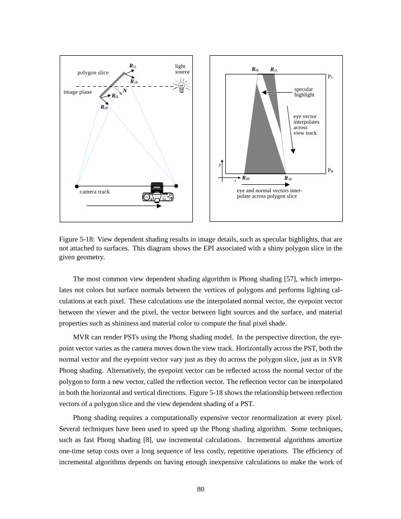
PL
PR
R1L
R0Rx
p
camera track
image plane
polygon slice
NR0L
R0R
R1L
R1R
R0L
R1R
eye and normal vectors inter-polate across polygon slice
eye vector interpolates across view track
lightsource
specularhighlight
Figure 5-18: View dependent shading results in image details, such as specular highlights, that arenot attached to surfaces. This diagram shows the EPI associated with a shiny polygon slice in thegiven geometry.
The most common view dependent shading algorithm is Phong shading [57], which interpo-
lates not colors but surface normals between the vertices of polygons and performs lighting cal-
culations at each pixel. These calculations use the interpolated normal vector, the eyepoint vector
between the viewer and the pixel, the vector between light sources and the surface, and material
properties such as shininess and material color to compute the final pixel shade.
MVR can render PSTs using the Phong shading model. In the perspective direction, the eye-
point vector varies as the camera moves down the view track. Horizontally across the PST, both the
normal vector and the eyepoint vector vary just as they do across the polygon slice, just as in SVR
Phong shading. Alternatively, the eyepoint vector can be reflected across the normal vector of the
polygon to form a new vector, called the reflection vector. The reflection vector can be interpolated
in both the horizontal and vertical directions. Figure 5-18 shows the relationship between reflection
vectors of a polygon slice and the view dependent shading of a PST.
Phong shading requires a computationally expensive vector renormalization at every pixel.
Several techniques have been used to speed up the Phong shading algorithm. Some techniques,
such as fast Phong shading [8], use incremental calculations. Incremental algorithms amortize
one-time setup costs over a long sequence of less costly, repetitive operations. The efficiency of
incremental algorithms depends on having enough inexpensive calculations to make the work of
80
setup worthwhile. An incremental algorithm used to render small polygons in SVR may not have
enough pixels to render to offset initial per-polygon costs. Since PSTs are larger than most polygons,
they may be more efficient to render using incremental techniques.
One disadvantage of using a technique such as fast Phong shading in MVR is that the accuracy
of shading may suffer. For example, fast Phong uses a Taylor series approximation of the exact
shading function to avoid the vector normalization. Taylor’s series is an exact approximation at a
central point in the function, but it is only approximate at other points of evaluation. The accuracy
can fall off quickly with distance from the central point. If the MVR viewing track is very long, the
range eyepoint vectors can cause a large variation in the parameters of the shading function, which
in turn can result in large errors in shading.
Reflection mapping
A more general technique for implementing a large class of view dependent shading is calledre-
flection mapping. Like texture mapping, reflection mapping introduces non-geometric detail into
a geometric scene. Rather than using surface coordinates to associate parts of a texture with parts
of the scene, a reflection map instead uses surface orientation to map the color of a reflection onto
the scene geometry. The environments that surround objects, such as sky, ground, and neighboring
objects, can be reflected in this way. Furthermore, specially designed reflection maps can be used
to simulate Phong shading of a surface.
Reflection maps can be implemented in several different ways. The most convenient ways
convert surface normal information into map indices that can be used with texture mapping to ap-
ply the reflection information to each surface. One implementation of this type of reflection map
technique, called spherical reflection mapping, converts the three-dimensional reflection vector into
a two-dimensional polar form, then indexes the coordinates into a specially-prepared environment
map. The map’s appearance is that of a shiny sphere seen from very far away: all directions of
reflection are represented somewhere in the map. In SVR, reflection-texture coordinates are com-
puted and assigned to each polygon vertex. The vertex texture information is linearly interpolated
by the texture mapping algorithm to fill the polygon.
MVR can use the same spherical reflection map algorithm to apply a reflection to a PST.
Reflection-texture coordinates are applied to each of the four PST vertices. Unfortunately, the wide
range of eyepoint vectors complicate this view depending shading algorithm. The first problem, as
Voorhies [72] points out, is the spherical reflection map’s susceptibility to texture wraparound. The
polar mapping used to convert the reflection vector into texture coordinates maps the far pole of
the reflection sphere to a circle, not a single point. Whenever an interpolated primitive’s reflection
spans the far pole, a small change in the reflection vector can cause a large change in the texture
coordinate of the image, and thus produce significant shading errors. In SVR, the problem does
not frequently occur because small polygons are unlikely to span much of the reflection sphere. In
81

MVR, a very long camera track may swing the reflection vector by up to 180 degrees. In such a
situation, many PSTs would likely span a pole. This problem can be reduced by using not just one
reflection map, but two: one constructed to favor the near pole of the reflection sphere, the other to
favor the far pole. Based on the average direction of the reflection vectors, a PST can be rendered
using one map or the other. Figure 5-18 shows a spherical reflection map pair.
Another problem with spherical reflection maps is that the produce only an approximation to
correct reflections. This property of approximation can be seen in the following simple example. If
two reflection vectors differing in only one directional component are interpolated, they sweep out a
great arc across the sphere of reflection. Projecting this arc from three to two dimensions using the
spherical texture mapping formula will also in general produce an arc through the reflection map
space. However, the spherical reflection map algorithm only calculates the texture coordinates of
the two endpoints of the curve, and linearly interpolates between them. The arc that passes through
the correct part of the reflection map is instead replaced by a straight line connecting the curve
endpoints. The two different interpolation paths are shown in Figure 5-20. For reflection vectors of
large variation, such as those seen in MVR, this error can produce noticeably incorrect reflections.
One way to minimize this distortion is to break up the long view track into smaller ones. In effect,
each PST is broken up into horizontal bands where correct reflection coordinates can be assigned to
the vertices of each. The arc through reflection map space is approximated in this way by a polygon,
but at the expense of more lighting calculations.
To eliminate this interpolation problem, MVR requires a reflection mapping algorithm where
linear interpolating between two reflection vectors and converting the result to reflection-texture
space produces the same results as converting to texture coordinates immediately and interpolating
the results. Voorhies describes an algorithm that has this property. Instead of using a flattened
sphere as a reflection map, the Voorhies algorithm maps the environment onto the planar faces of a
cube that surrounds the object. Although the possibility is not described in the paper, the reflection
from a single light source or other localized reflection can be implemented with just a single flat
oriented plane. Such a plane is shown in Figure 5-21.
82

forward facing
backward facing
Figure 5-19: A pair of spherical reflection maps is used to minimize the problem of reflectionwraparound in reflection mapped MVR-rendered images.
83

incorrect linear interpolation
correct sphericalinterpolation
Figure 5-20: Interpolation errors occur when texture coordinates that correspond to reflection vec-tors are linearly interpolated. Correct interpolation would either linearly interpolate the vectorsor interpolate the texture coordinates in a spherical coordinate space. For large ranges of cameramotion, the errors in shading can be significant.
Figure 5-21: A planar reflection map representing the effect of two light sources.
84

One of the important parts of Voorhies’ cubical reflection map algorithm is the efficient way
that it computes and uses unnormalized reflection vectors. A formulation is given that calculates
the unnormalized reflection vectorR given an eyepoint vectorE and surface directionN vectors
(which can also have non-unit length):
R = 2N(N �E)� E(N �N)
The rendering algorithm never needs to normalize the reflection vector. IfR has components
(x; y; z), the texture coordinates for one of the planes of the cube is given by(s = xz; t = y
z),
wheres andt are independent of the magnitude ofR. A texture matrix can be used to transform
R into the coordinate system of the reflection plane. The ratio operation can be implemented using
the homogeneous division hardware used in texture mapping.
Reflection mapping, just like texture mapping, must be done with consideration of perspective
foreshortening of the surface onto which the reflection appears. As Voorhies suggests, perspective
correction can be performed by premultiplying the texture coordinates derived fromR by 1
w, the
inverse of the geometric homogeneous coordinate. The homogeneous reflection-texture can be lin-
early interpolated freely and only converted back to an true texture coordinate at the pixel level.
This interpolation process is called hyperbolic interpolation [10]. The conversion to(s; t) texture
space happens automatically when the ratios of the reflection components are taken:1
wcancels out
from both numerator and denominator of the fraction.
Another convenience of the unnormalized vector formulation is the resulting linear relationship
between eyepoint and reflection vectors. The following equation shows this linear relationship:
R(N;E+ �dE) = 2(N � (E+ �dE))N� (N �N)(E+ �dE)
= 2N(N �E) + 2�N(N � dE)� (N �N)E� �(N �N)dE
= 2N(N �E)� (N �N)E+ �[2N(N � dE)� (N �N)dE]
= R(N;E) + �R(N;dE) (5.2)
Furthermore, letE0 be a fixed eyepoint vector,�Ex be an incremental step of the eye vector
in thex direction, and�Ey a step of the eye vector in they direction. Any motion of the PRS
camera viewpoint produces an eye vector
E = E0 + x�Ex + y�Ey
Given this eye vector, the resulting reflection vectorR is given by the following equation:
R = R(N;E0) + xR(N; �Ex) + yR(N; �Ey)
85

In other words, the relationship betweenE andR is separable. Separability will be important later
when the implementation of full parallax MVR is considered. The linear relationship between the
eyepoint vector and the reflection vector also means that the incremental reflection vectors can be
prescaled by the inverse homogeneous coordinate with correct results:
1
wR =
1
wR(N;E0) + x
1
wR(N; �Ex) + y
1
wR(N; �Ey)
The remaining step of the process is to demonstrate that the projection of the three-dimensional
vector onto two-dimensional texture space preserves straight lines. This property can be shown
by observing that the operation of computing the ratio of the reflection components performs a
projection of the three-dimensional vector onto the cubic texture plane. As long as the reflection
vector has non-zero magnitude, the projection operation always preserves straight lines.
The linear relationship of the eyepoint vector and reflection vector and the straight-line pre-
serving property of the projection operation imply that the cubic reflection map algorithm does not
introduce the spherical distortions that occur in the spherical reflection map algorithm. Unfortu-
nately, the algorithm as presented by Voorhies was designed to use special operations not currently
implemented in existing hardware graphics systems. One of these operations is a three-way compar-
ison operation used to decide into which texture map a reflection vector should index. Difficulties
arise when the algorithm is implemented on existing systems that do not have these special features.
Details of these problems will be presented in the implementation section.
Reflection mapping, whatever technique is used, requires that reflection map coordinates be
computed at every vertex in the scene. An exact implementation of reflection mapping would find
the eyepoint vector by subtracting each vertex position from the position of the camera. In this case,
every vertex will have a slightly different eyepoint vector. A simplification of this calculation finds
one representative eyepoint vector for every perspective viewpoint, perhaps between the centroid of
the object and the camera location. This approximation effectively moves the viewer to a distant po-
sition for the purposes of shading. Since the eyepoint vector still varies with respect to perspective,
reflections still move with respect to the surfaces on which they are seen.
5.6.9 Combining different shading algorithms
Most scenes are made up of a number of different materials, and most materials are not exclusively
specular or diffuse but a combination of the two. Modeling real-world scenes requires a way to
combine different shading models and results to form composite shading functions. The simplest
way to combine the shading methods previously described (Gouraud shading, texture mapping,
reflection mapping, and other view dependent shading techniques) is to render each in a separate
rendering pass. Separating the different techniques allows, for example, texture mapping algorithms
to be used to implement both texture mapping and reflection mapping. In the case of view depen-
86

dent shading, the effect of different light sources or environments may require a series of different
rendering passes.
The implementer of multi-pass rendering can choose to process the entire scene in one pass
after the other, or to render all the passes for each EPI before moving on to the next. The second ap-
proach is usually preferred because the scanline slice table only needs to be traversed once. In either
case, though, the result of the multiple rendering passes are usually summed using anaccumulation
buffer or blending hardware.
5.6.10 Image data reformatting
After the rasterization process has produced a complete spatio-perspective volume, the image data is
ready for the next step in the imaging pipeline, be it additional processing operations, data storage,
or immediate display. The epipolar plane image volume is produced by MVR one EPI at a time.
In other words, the first scanline from each of the perspective images is rendered, then the second
scanline, then the third, and so on. The naturalEPI-major ordering of the data is different than
theviewpoint-majorordering that is natural for SVR. If an MVR renderer is required to produce
compatible viewpoint-major data, scanlines of the output images must be reshuffled in memory or
on disk. Reshuffling can be expensive in terms of memory or I/O costs, so ways to avoid it should
be considered if possible.
Many of the applications for which MVR is well-suited can use data in EPI-major format, ob-
viating the need to rearrange data. For instance, a raster-scanned disparity-based three-dimensional
display such as a CRT-driven panoramagram, or a holographic video system [62], most likely scans
out data in EPI-major order. If the rendering process is fast enough, the display subsystem can be
scanning out one line of the image while MVR can be generating the data for the next one.
Other display pipelines may require that the rendered image data be manipulated further before
it is suitable for final display. One example of this kind of post-processing is precompensation for
optical distortions that the display introduces [33]. In HPO displays, most of these distortions are
restricted to the horizontal direction and therefore lie in epipolar planes. As a result, distortion cor-
rection can often be done by predistorting EPIs. Since the rendering, predistortion, and display are
independent, the three operations can occur in parallel on different scanlines of the image volume.
The latency of the now-parallel display process is also greatly reduced. A further discussion of im-
age predistortion and opportunities for parallelization is included in the applications and extensions
chapter.
Finally, some applications that require viewpoint-major images may be able to perform image
reformatting as part of another process. For instance, an imaging pipeline that stores its data in
secondary storage, such as on a disk, might write data to disk in EPI-major format, but read it back
from disk scanline by scanline to build up viewpoint-major format images. A scanline of data is
87

usually long enough that retrieving them from disk is efficient. Sequential reads only require a
disk seek between them. This technique masks the cost of reshuffling data behind the larger cost of
disk access. Another example of this kind of application is image based rendering. The image based
rendering algorithm can potentially traverse a large amount of image memory building up the pieces
of a single arbitrary viewpoint. In this case, the reshuffling operation effectively happens during
every extraction. The order in which that data is originally generated is thus only of secondary
importance.
5.6.11 Full parallax rendering
The MVR algorithm described so far produces only a linearly varying range of perspectives using an
LRS camera, not a two-dimensionalmatrix of views. In theory, the additional perspective coherence
of full parallax would further increase the efficiency of the rendering process. Object details would
sweep out a two-dimensional surface in the hypervolume of camera views, while polygons could
be rendered from all viewpoints at once by scan-converting the four-dimensional volume that lies
between the surfaces defined by the polygon’s vertices.
There are several reasons why such an implementation of full parallax rendering is currently
impractical. First, a typical three-dimensional image array is too big to fit into primary memory on
many computer systems. Because of the order in which MVR renders its image data, producing per-
spective images is costly if image memory is not available by random access. Many of the benefits
of two-dimensional perspective coherence would be lost to swapping on machines with insufficient
memory. Second, a true full parallax MVR algorithm is poorly suited to hardware acceleration
on today’s memory-limited graphics subsystems. The memory constraints for hardware rendering
systems are even more severe than for primary computer memory: only a small amount of image
information can be processed at one time. Full parallax MVR implemented using existing hard-
ware requires that the higher dimensional spatio-perspective volume be broken down into a series
of two-dimensional images, resulting in no extra computational saving from the extra coherence.
The simplest way to produce the two-dimensional perspective image matrix of a PRS camera is
to render a series of one-dimensional perspective image sequences using horizontal parallax MVR.
The PRS grid is decomposed into a series of LRS camera tracks. To produce each sequence, the
scene’s polygons must be retransformed, resliced and rerendered. Pre-calculation can reduce the
cost of this repeated operation by taking advantage of the PRS geometry. For example, retrans-
forming the polygons from one HPO image subsequence to another can be much less expensive
than a full matrix multiply per point. From one vertical camera position to another, the screen po-
sition of a vertex varies regularly, and only in the y direction. This vertical per-viewy delta can
be pre-calculated; to transform a vertex from one horizontal row of images to the next, a vertex’sy
coordinate is incremented by this delta. Retransformation can thus be done at a cost of one addition
per vertex.
88

Conveniently, texture map coordinates do not change from one vertical perspective to another,
just as texture coordinates do not shift across surfaces. Reflection coordinates, in contrast, change
with vertical as well has horizontal perspective. The separability of the relationship between the
reflection and eyepoint vectors can be used to incrementalize the reflection vector calculation. The
change in eyepoint between two adjacent vertical perspectives can be used to precalculate the incre-
mental reflection vector at the time of vertex transformation. To recalculate the reflection vector for
each new vertical perspective, only one vector addition is required. For a reflection-mapped scene,
the total cost of retransforming the scene vertices for each new horizontal image sequence is thus
only four scalar additions per vertex.
This chapter has described the properties of the spatio-perspective space that are useful for
rendering as well as specific techniques that MVR uses to efficiently render the spatio-perspective
volume. The next chapter looks more closely at implementation details of the MVR algorithm.
89

Chapter 6
Implementation details
This chapter describes constraints and other considerations arising from a prototype implementation
of the MVR algorithm. Some of these issues result from inherent characteristics of MVR. Others are
due to practical limitations of this implementation, including constraints imposed by the graphics
hardware used to render MVR primitives. Details of both types of issues will be discussed here.
6.1 Basic structure
The MVR implementation described here is composed of four distinct elements:
� data input and conversion to standard form
� per-sequence geometry processing
� device-dependent rasterization
� output of pixel data to files or displays
This organization is convenient because the details of file conversion and image data handling,
which may change depending on the application, are separate from the more basic rendering compo-
nents. Furthermore, the calculations done once per image sequence are for the most part independent
of the underlying graphics library. The operation that are performed once per EPI are more closely
tied to the graphics library used for implementation. In the case of the prototype implementation,
this graphics library is OpenGL [11], as implemented under the IRIX 5.3 operating system running
on Silicon Graphics computer systems. If support for another similar library were desired, most of
the changes could be made in the device-dependent module of the prototype implementation. The
steps of the pipeline are shown in Figure 6-1.
90

modeler
geometrycreation
textureassignment
color assignment
input
geometryformatconversion
per-sequenceoperations
geometrytransformation
polygon slicing
per-EPI operations
slice to PST conversion
device-dependentoperations
rasterization
output
image data reformatting
incremental operations setup
other imagingand displaystages
MVR
Figure 6-1: A block diagram of the high-level modules used in the prototype MVR implementation.
6.2 Before the MVR pipeline
The prototype implementation of MVR was designed for compatibility with the scene geometry
generated by the Alias Studio modeling program from the Alias/Wavefront Division of Silicon
Graphics, Inc. Alias Studio is used both by our laboratory but also by many of our sponsors and
collaborators in the automobile industry. The Alias Studio modeler allows the user to create, import,
and manipulate higher-level graphics primitives such as non-uniform rational B-spline (NURBS)
patches to design complicated objects and scenes. Fortunately, one of the modeler’s output options
converts all of these primitives into simple independent triangles. The degree to which the model is
tessellated to form the triangle database can be controlled by the user.
The modeler uses lighting and texture effects applied by the user to calculate per-vertex colors.
By disabling view dependent shading effects in the modeler, all view independent shading can be
included in the model’s vertex color information This function of the modeler eliminates the need
for MVR to perform these calculations. Reducing the complexity of the MVR renderer increases
the chances that the final rendered image will match model that the user created.
6.3 Scene input
The input stage is responsible for interfacing the MVR program to external modeling and scene
generation programs and for converting their output into a standardized form stored in random
access memory. The internal form consists of a set of independent triangles, with each triangle
vertex described by a three-dimensional location, a color, a directional orientation, and a texture
coordinate. Since the triangles are independent and not arranged in a strip or grid, each vertex is
replicated three times. This arrangement was easiest to prototype because it is directly compatible
with the Alias Studio output; more efficient implementations could construct and use a shared-vertex
geometry description.
91

V0,0 V0,1
V1,0
V0,m-1
Vn-1, m-1Vn-1,0
V1,m-1
horizontal parallax (HPO MVR, m views)
vertical parallax(n separate
HPO sequences)
Figure 6-2: Full parallax MVR is implemented as a series of horizontal parallax image sequences,indicated by the solid black lines. Geometric transformations and shading parameters can be com-puted at selected viewpoints and interpolated to find values at all other viewpoints. The large blackdots indicate viewpoints that correspond to view transformation matrices.
6.4 MVR per-sequence calculations
6.4.1 Per-vertex calculations
The first rendering step of the MVR algorithm proper precalculates per-vertex information used
throughout the view sequence. Per-vertex data includes vertex locations, view independent shading
information, and texture coordinates for both texture and reflection mapping. Each of these parame-
ters is computed in such a way that the results can later be linearly interpolated, first to find polygon
slice endpoint values, then to find values for interior points within a PST. The prototype implemen-
tation is designed to generate images for a full parallax geometry using multiple horizontal parallax
image sequences; vertex precalculation includes computing parameters that describe vertical paral-
lax as well as horizontal. For reference, Figure 6-2 shows the arrangement and designations of the
viewpoints that make up the different image sequences in a full parallax rendering.
Lateral motion of a shearing camera results in the apparent motion of scene vertices only in
the direction of that motion. Because of this fact, only two transformation matrices are required
92

to describe the range of viewpoints of a PRS camera geometry: one corresponding to an origin
viewpoint, the other to a viewpoint offset both horizontally and vertically from the first. In Figure 6-
2, the corresponding view positions are labeledV0;0 andV1;m�1.
A point (x; y; z) transformed by the matrix derived fromV0;0 has following coordinates:
(x0;0; y0;0; z0;0; w0;0):
Similarly, transformation from pointV1;m�1 yields
(x1;m�1; y1;m�1; z1;m�1; w1;m�1):
The coordinates of the point when viewed from other important locations can be derived from these
two transformations. For example, the coordinates for viewpointsV0;m�1 andV1;0 are given as
follows:
V0;m�1 ) (x1;m�1; y0;0; z0;0; w0;0)
V1;0 ) (x0;0; y1;m�1; z0;0; w0;0)
The transformation matrices corresponding toV0;0 andV1;m�1 are computed from view pa-
rameter information provided in a configuration file. The redundant information is removed, leaving
only the terms necessary to find the following coordinates:
(x0;0; x1;m�1; y0;0; y1;m�1; z0;0; w0;0)
this expression can be abbreviated unambiguously as:
(x0; xm�1; y0; y1; z0; w0)
wherex0 is thex coordinate of the vertex seen from the first view of the first horizontal image
sequence,xm�1 thex coordinate from the last view of the same sequence, andy1 is they coordinate
seen from the first view of the second horizontal image sequence.
Each scene vertex is transformed using the pair of transformations fromV0;0 andV1;m�1. Be-
cause of the reduced redundancy of the calculation, transforming a vertex costs approximately 1.5
matrix multiplies. The homogeneous divide, which should happen by this point, is also less expen-
sive than that required for two independent points.
To incrementalize the calculation of new vertex positions through the rendering process, the
transformed geometry is stored as initial values and incremental offsets:
(x0;�x; y0;�y; z; w)
93

�x and�y have slightly different meanings:�x is the difference betweenx coordinates across the
entire range of horizontal perspectives, while�y is the difference from one vertical perspective to
another. These differences reflect how the two values are used during rendering.
Assigning view independent shading and texture coordinates to vertices is straightforward be-
cause these values do not vary with perspective. Typically, color is interpolated linearly, not hy-
perbolically, across polygons since the eye seldom notices errors in shading due to foreshortening.
Texture coordinates, which must be interpolated hyperbolically, are assigned in a form compatible
for linear interpolation as follows:
(s0; t0; q) =
�s
w;t
w;1
w
�
Reflection coordinates are view dependent parameters: the direction of the reflection vector
varies with perspective. A change in viewpoint in one direction can result in the reflection vector
changing in another, even though the relationship between the reflection and eye vector is separable.
For each reflection-mapped vertex, reflection vectors must be computed from three viewpoints,
where two of the points are offset strictly horizontally and two strictly vertically. The two vector
differences between these pairs of reflection vectors are the incremental change due to viewpoint.
one difference vector represents the change due to horizontal observer motion, the other due to
vertical. Both vectors are stored for all reflection-mapped vertices.
6.4.2 Polygon slicing
Polygon slicing uses the transformed scene geometry to form a set of data structures representing the
intersection of each triangle with each scanline. The position and values of the shading parameters
at the slice endpoints are determined by interpolation of the per-vertex values.
A scene with many large polygons could, when sliced, result in a very large slice database.
If the slice data structure stored the interpolated values of the endpoints directly, the memory re-
quirements for storing the slices could well exceed reasonable levels. To avoid this problem, the
prototype implementation instead uses an indirect data structure that refers to triangle vertices and
their values instead of storing them directly. Figure 6-3 is a pictorial representation of a slice data
structure. Each slice is represented by ay coordinate, three references to triangle vertices, and two
scalar interpolation constants. The three vertex references describe the two edges of the triangle
upon which the two endpoints of the slice lie. The two edges share the vertex referenced to by
�Vs, with the first endpoint lying between�Vs and�V� and the other falling between�Vs and�V�.
The scalar interpolation parameters� and� specify the normalized position of the respective slice
endpoint between the two edge vertices.
The interpolation parameters� and� are used to find the parameter values for each polygon
slice endpoint. IfP represents a shading parameter for a given vertex, the value forP at the slice
94

α
β
(1−β)(1−α)
V0
V2
V1
E0 E1
*Vα *Vβ*Vsα βy
P(E0) = (1-α)P(*Vα) + αP(*Vs)
P(E1) = (1-β)P(*Vβ) + βP(*Vs)
slice data structure
slice
trianglefrom scene
Figure 6-3: MVR’s slice data structure contains references to vertices in the scene database, aswell as interpolation parameters specifying the location of the slice endpoints with respect to thosevertices.
95

endpoints can be found using the following relation:
P (E0) = (1� �)(�V�) + �(�Vs)
P (E1) = (1� �)(�V�) + �(�Vs)
In this way, the values for all linearly interpolated parameters can be calculated without the need to
store the results explicitly for all slices in the database.
Slices are formed by point sampling each triangle based on its projection into screen space, at
intervals corresponding to the height of a scanline. The exact location of scanline intersection, and
the number of slices per polygon, is dependent on vertical viewpoint. As a result, the slice database
must be recalculated for every horizontal parallax image sequence that composes a full parallax
rendering sequence.
As the slices for each polygon in the scene database are formed, they are inserted into a database
called ascanline slice table. The slice table has one entry for every horizontal scanline of the image,
stored in order from bottom to top. Every table entry holds a list of the polygon slices that intersect
the corresponding scanline. Once an entry in the slice table has been filled, it contains all the
geometric information required to render the EPI for that scanline. Inserting the slices from each
polygon into the table as they are generated eliminates the need to later sort the entire table.
Once the scanline slice table has been constructed, each EPI is rendered in turn. Here we
consider the sequential rendering of EPIs; a multiple processor computer system could possibly
render several EPIs simultaneously.
In order to be rendered in spatio-perspective space, the polygon slices that intersect each scan-
line must be converted into PSTs that can be rendered into the EPI. Current graphics systems do not
directly rasterize PSTs, so the PST description must be converted into other graphics primitives that
can be rasterized. In order to simplify experimentation with different graphics primitives, the proto-
type implementation explicitly converts polygon slices to PSTs, then passes the PST data structures
to a graphics system-dependent rendering module. The next section describes how the rasterization
of PSTs has been implemented.
6.5 Device-dependent rendering
Up until this point in the rendering pipeline, all of MVR’s computational costs incurred have been
independent of the number of perspective views in the final image. In fact, the scene representation
is still continuous and geometric in the horizontal and perspective directions. Once the rasterization
process begins, rendering costs become dependent on the number of views produced, if only because
more pixels have to be drawn onto the screen or into memory. The goal is to find a way to render a
96
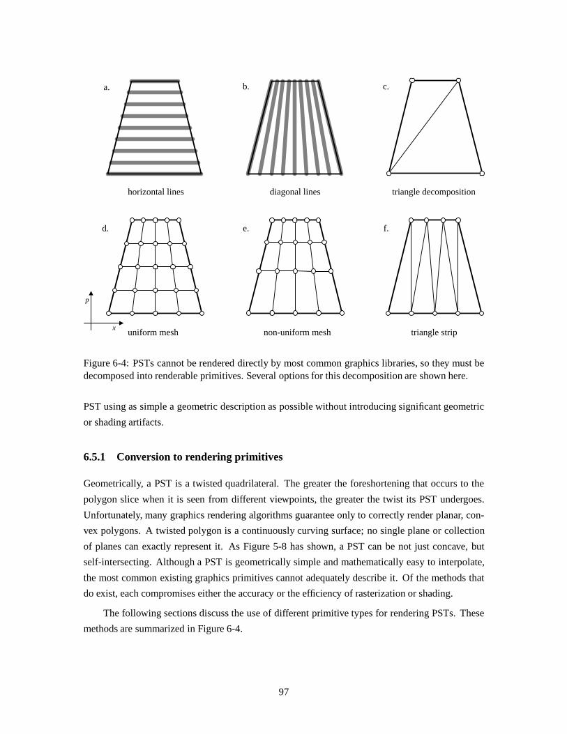
x
p
a. b. c.
d. e. f.
horizontal lines diagonal lines triangle decomposition
uniform mesh non-uniform mesh triangle strip
Figure 6-4: PSTs cannot be rendered directly by most common graphics libraries, so they must bedecomposed into renderable primitives. Several options for this decomposition are shown here.
PST using as simple a geometric description as possible without introducing significant geometric
or shading artifacts.
6.5.1 Conversion to rendering primitives
Geometrically, a PST is a twisted quadrilateral. The greater the foreshortening that occurs to the
polygon slice when it is seen from different viewpoints, the greater the twist its PST undergoes.
Unfortunately, many graphics rendering algorithms guarantee only to correctly render planar, con-
vex polygons. A twisted polygon is a continuously curving surface; no single plane or collection
of planes can exactly represent it. As Figure 5-8 has shown, a PST can be not just concave, but
self-intersecting. Although a PST is geometrically simple and mathematically easy to interpolate,
the most common existing graphics primitives cannot adequately describe it. Of the methods that
do exist, each compromises either the accuracy or the efficiency of rasterization or shading.
The following sections discuss the use of different primitive types for rendering PSTs. These
methods are summarized in Figure 6-4.
97

Horizontal lines
A PST can be represented as a set of horizontal lines, one per scanline, that interpolate geometric
and shading parameters from one endpoint to another. This rendering method is exact: values of
parameters vary correctly across each line, and the geometry of the shape matches the ideal PST.
For efficiency, scanline-aligned horizontal lines are relatively simple for scan conversion hardware
to draw. Also, no pixel that is part of the PST is ever drawn more than once, which may minimize
the cost of hidden surface removal and permit parallelization.
The horizontal line technique has the disadvantage that the number of primitives that must be
drawn to fill a PST is large, and linearly proportional to the number of perspective images to be
rendered. The number of vertices passed to the graphics subsystem to describe the lines would
be the same as if an SVR algorithm filled each polygon using a set of horizontal lines. Filling
primitives using horizontal lines would not only fail to increase the pixel to vertex ratio�, it would
significantly decrease it for most scenes.
Diagonal lines
Another line drawing technique for rendering PSTs draws diagonal lines that connect the two p-
edges of the PST. The diagonal lines are interpolations of the two i-edges, gradually changing
in slope from one i-edge to the other. Each line has a constant depth value, shade, and texture
coordinate. The number of diagonal lines required to fill a PST is dependent on the pixel width of
the longer p-edge.
The diagonal line algorithm has the advantage that the number of primitives drawn is not de-
pendent on the number of viewpoints to be rendered. Scenes with small polygons viewed from
many different viewpoints can be filled with a small number of diagonal lines. Drawing constant
shaded lines is also a relatively fast operation.
On the other hand, diagonal lines are more costly to draw than strictly horizontal or vertical
ones. A single pixel of a PST image may be painted by several different lines. Care must be taken
to assure that line rasterization fills all pixels of the PST, leaving no holes. Improper filtering of the
lines may produce moire patterns and other aliasing artifacts. A diagonal line drawing algorithm
cannot draw primitives narrower than its line width. As a result, if a PST intersects itself, the
algorithm will incorrectly render the perspectives close to the intersection point.
Quadrilaterals and triangles
Surfaces are generally preferable to lines for filling operations because they eliminate the prob-
lems of gaps, holes, or repeated pixel repaints. Surfaces can also be more efficient in terms of the
pixel to vertex ratio. The most obvious choice of surface primitive for rendering PSTs is a single
98
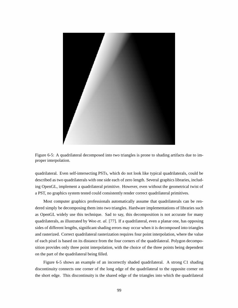
Figure 6-5: A quadrilateral decomposed into two triangles is prone to shading artifacts due to im-proper interpolation.
quadrilateral. Even self-intersecting PSTs, which do not look like typical quadrilaterals, could be
described as two quadrilaterals with one side each of zero length. Several graphics libraries, includ-
ing OpenGL, implement a quadrilateral primitive. However, even without the geometrical twist of
a PST, no graphics system tested could consistently render correct quadrilateral primitives.
Most computer graphics professionals automatically assume that quadrilaterals can be ren-
dered simply be decomposing them into two triangles. Hardware implementations of libraries such
as OpenGL widely use this technique. Sad to say, this decomposition is notaccurate for many
quadrilaterals, as illustrated by Wooet. al. [77]. If a quadrilateral, even a planar one, has opposing
sides of different lengths, significant shading errors may occur when it is decomposed into triangles
and rasterized. Correct quadrilateral rasterization requires four point interpolation, where the value
of each pixel is based on its distance from the four corners of the quadrilateral. Polygon decompo-
sition provides only three point interpolation, with the choice of the three points being dependent
on the part of the quadrilateral being filled.
Figure 6-5 shows an example of an incorrectly shaded quadrilateral. A strong C1 shading
discontinuity connects one corner of the long edge of the quadrilateral to the opposite corner on
the short edge. This discontinuity is the shared edge of the triangles into which the quadrilateral
99

is decomposed. The error is manifested not just in color but in all parameters interpolated across
the surface. The problem can change geometry as well as shading: the error affects the interpo-
lated depth values of each pixel, which can result in incorrect hidden surface removal. Errors are
minimized for scenes with small polygons, for areas of small variation in color or texture, or for
relatively small ranges of viewpoint.
Polygon meshes
More accurate polygonal approximations require further subdivisionsof the PST into smaller pieces.
Smaller polygons yield reduced shading error, but require more vertices to describe. Meshes reduce
the number of vertices required to describe a primitive because interior vertices of the mesh are
shared between polygons.
The most obvious tessellation of a PST is formed by covering it with a uniform polygonal
mesh. Uniform spacing is not optimal for reducing shading artifacts, though. Errors in quadrilateral
shading are proportional to the ratio between the length of their two sides. This ratio varies geomet-
rically over the height of the PST, not linearly. A uniform grid over-tessellates the wide parts of a
PST where the ratio changes slowly, and under-tessellates the narrow parts where it changes more
quickly. A non-uniform tessellation using a geometrically increasing spacing reduces the number
of subdivisions needed.
Linear patches
OpenGL simplifies the process of subdividing the PST into a polygonal grid by providing a surface
patch primitive. A PST can be described as a linear surface patch to the graphics library. Although
linear surface patches are somewhat unusual in computer graphics, libraries such as OpenGL im-
plement them as a more primitive case of higher order surfaces patches. The degree of tessellation
of the patch, whether uniform or non-uniform over the patch, can be specified as a parameter when
the patch is rendered.
The surface patch primitive is very convenient for specifying the PST, and future implementa-
tions of OpenGL could be optimized to render linear patches using only interpolation, without Tess
elating them into polygons at all. At the current time, however, surface patches are not used as often
as polygon meshes or triangle strips. Consequently, this primitive appears to not be optimized as
heavily as the more oft-used primitives.
Triangle strips
A tessellated surface patch can always be replaced by the geometrically identical triangle strip or
mesh. A triangle strip of sufficient density is in fact very similar to a set of horizontal or diagonal
100

inaccurate two-triangle interpolation
accurate interpolation
0.0 0.1 0.25 0.5 0.75 1.0
Figure 6-6: Adaptive triangle strip decomposition correctly shades PSTs compared to the artifactsintroduced by simple triangle decomposition.
lines, except it can be rendered without holes or redrawn pixels. The degree of tessellation of
a triangle strip determines the accuracy of the PST’s shading. A triangle strip consisting of tall,
slender triangles is preferable to one made up of short wide ones because the primitive count is
independent of the number of viewpoints rendered. Small polygon slices may only require a few
triangles to fill them entirely.
Adaptive tessellation
One final optimization of polygon tessellation can be made by adaptively decomposing each PST
based on its individual twist. Since a difference in the lengths of a PST’s p-edges can only occur be-
cause of twist, an untwisted PST has p-edges of identical length and can be rendered with only two
triangles. Most scenes have a significant fraction of polygons that face towards the viewer. These
polygons correspond to PSTs that have little or no twist and that do not demand dense polygonaliza-
tion when being rendered. The further from unity the ratio between the lengths of the two p-edges
is, the greater the amount of tessellation required. The upper limits of tessellation is determined by
the pixel width of the wider p-edge. Figure 6-6 shows the difference in shading error between a
set of PSTs rendered using simple triangle decomposition and another using adaptive triangle strip
decomposition.
The prototype implementation permits a user-defined choice of PST rendering between the
efficient but error-prone quadrilateral approximation and the slower but more correct adaptive mesh
decomposition. The adaptive mesh method is implemented using the linear surface patch primitive
available in OpenGL. The fast quadrilateral method is useful as an indicator of MVR’s maximum
101

performance. For most of the scenes rendered for performance tests, in fact, the shading artifacts
were not very noticeable because the polygons were small and usually had slowly varying shading
across their surface. On the other hand, adaptive mesh decomposition produced hardware-related
artifacts unrelated to the primitives themselves on one test system. Performance on this system was
also poor for linear surface patches. This fact seems to indicate that the part of the hardware pipeline
that deals with linear surface patches on this system was not as well used, tested, or optimized as
the polygon rendering pipeline.
6.5.2 Texture mapping
Texture mapping is supported in the prototype implementation by assigning the texture coordinates
of the polygon slice endpoints to both ends of the corresponding PST i-edge. The implementation
relies on the underlying graphics library to render the texture using conventional MIP-based texture
mapping. The MVR-optimized texture mapping operation described in the MVR algorithm chapter
is not incorporated into the prototype implementation. When possible, a user-defined texture map
is used to determine per-vertex colors of the model before MVR begins. While applying texture in
this way negates many of the advantages of texture mapping, it does an effective job of producing
rendered images that match the user’s textured model.
6.5.3 Reflection mapping
Both spherical and planar reflection mapping are implemented in the prototype rendering system.
Reflection mapping is perhaps the one area where limitations of the graphics library with respect to
MVR are the most glaring. Neither algorithm provides distortion- and artifact-free images over a
wide viewpoint range without subdivision of the PST graphics primitives.
The spherical reflection mapping implementation converts the per-vertex reflection vectors into
spherical texture coordinates just before PST rendering. The reflection vectors corresponding to the
left and right eyepoints are first normalized, then scaled by the inverse homogeneous coordinate
value 1
w. Thez values of the reflection vectors for each corner of the PST are used to vote on whether
the forward or reverse reflection sphere is used as a map. Based on this choice, the reflection map is
converted to the appropriate two-dimensional spherical texture coordinates. The reflection mapping
facilities built into the OpenGL library are not directly used, although the process of reflection
mapping is effectively the same.
The quality of the spherically reflection mapped images is quite good, provided that the view
track length is limited no more than approximately the distance between the camera and the object.
The transition point between the front and rear reflection spheres is sometimes noticeable. Planar
reflection mapping produces fewer distortions of the reflections in the image, but suffers artifacts
from the lack of complete hardware support. To implement planar reflection maps, the reflection
102

vectors for the PST are used directly as texture coordinates. The texture transformation matrix
provided by OpenGL transforms the coordinates of each reflection vector into the coordinate system
of each of the planar reflection maps. The transformation is performed in such a way that the
major or prevailing axis of the reflection vector in the map’s coordinate space is loaded into the
homogeneous coordinate of the texture value. The hardware-provided perspective texture divide
performs the requires vector ratio operation, projecting the vector onto the map.
Unfortunately, two different reflection vectors map to every texture coordinate:(x; y; z) and
(�x;�y;�z) both map to(xz; yz). The Voorhies algorithm has a separate hardware element to dis-
tinguish the major axis of each reflection vector, which differentiates between these two cases.
Without this element, the ambiguity of the reflection vector to texture coordinate mapping can
produce severe interpolation artifacts when a PST’s reflection vectors span a significant range of
direction. OpenGL also provides no clipping of primitives with negative homogeneous texture co-
ordinates. These limitation effectively impose the same limits on viewpoint range that are required
for artifact-free spherical reflection mapping. If the hardware system described by Voorhies is ever
commercialized, MVR will be able use it directly for arbitrary reflection mapping.
6.5.4 Hidden surface removal
Hidden surface removal in the prototype implementation uses the depth buffer algorithm performed
by the underlying graphics library and perhaps by underlying graphics hardware. Thez coordinate
of the polygon slice is scaled by the transformation process to range between0 at the near and1 at
the far depth plane. The normalizedz value is scaled by the graphics library to span an algorithm-
or hardware-dependent integer depth range. Depth buffering in the EPI plane preserves the natural
depth relationship between polygon slices.
6.5.5 Multiple rendering passes
The combination of view independent color, texture mapping, and multiple reflection mapping ren-
dering passes is implemented using an accumulation buffer provided by the graphics library. The
accumulation buffer is an invisible memory buffer of greater numerical precision than the pixel
values from any one rendering pass. As each pass is rendered, its contribution is added to the accu-
mulation buffer. A scaling factor is applied if necessary to prevent overflow of pixel values. Each
rendering pass typically contributes a mathematically equal fraction of the appearance of the final
image. In some cases, such as if several independent light sources illuminate different parts of the
scene, a group of rendering passes could be accumulated with unequal scaling. Once accumulation
of all rendering information is complete, the composite image information is read back into the
display memory where it can be accessed just like any other image.
103

Figure 6-7: Nine images from a larger full-parallax image set, showing the combination of texturemapping and reflection mapping using the accumulation buffer.
Figure 6-7 shows a 3�3 grid of images taken from a 16�3 image full-parallax rendering of
a texture mapped and reflection mapped Ferio. Texture mapping was performed using MIP map
texture coordinates applied to the vertices of each PST. Reflection mapping was done using the
spherical reflection mapping technique. The two rendering passes were composited using the accu-
mulation buffer.
6.6 Output
As the graphics subsystem renders each EPI, it stores the results in display memory. EPI images are
of little use to a user seated in front of a graphics workstation; to convert the data into a usable form,
it must normally be read back into the computer’s main memory and stored on disk or manipulated
by another stage of the imaging pipeline. A very small number of applications may be able to
decode the video signal of the framebuffer directly as a means of using the EPI image information.
The output stage of the prototype implementation is designed for convenient inspection of the
rendered data without the need to store or examine every perspective. Any single perspective image
can be selected from a sequence, or the entire sequence can be stored. In addition, all output can be
disabled in order to test the speed of the rendering process without delays caused by disk or network
limitations.
104

Image sequences are stored in a single file using a variant of the “portable pixmap” (PPM)
format. The PPM format has a simple string-based header followed by an array of unencoded three-
byte binary values specifying the color of each pixel. PPM supports arbitrary comment lines in the
header of the image; MVR inserts a special comment line describing the number of viewpoints, both
horizontal and vertical, in the viewpoint array. Storage can be either in EPI-major or viewpoint-
major order, depending on the order in which the data is generated. A special flag in the PPM
comment indicates in which order a particular file is stored. It is the responsibility of the program
that reads the file to correctly interpret the data as either a collection of EPIs or perspective views.
6.7 Full parallax rendering issues
As previously mentioned, the full parallax rendering method that this MVR algorithm uses does not
take advantage of the additional perspective coherence found in the vertical dimension to increase
the efficiency of rendering. Significant computational savings do result, however, from the per-
vertex precalculations that take place at the beginning of the MVR pipeline. The incremental delta
values stored at each vertex during initial transformation, a result of the regular motion of the PRS
camera, reduce the cost of moving from one horizontal parallax image subsequence to the next.
After a horizontal parallax image subsequence is completed and its image data stored, all MVR
data structures other than the scene triangle database must be reinitialized. First, the position ofeach
scene vertex must be recalculated for the new vertical viewpoint position. The currenty coordinate
of each vertex is incremented by the corresponding�y for that vertex. Similarly, the current reflec-
tion vector is incremented by the vertical difference reflection vector at each vertex. All other vertex
parameters are constant with respect to a change in vertical viewpoint; thus, they require no update
from one horizontal subsequence to the next.
Using this incremental technique, each vertex can be transformed quite inexpensively using
approximately seven additions. If the incremental technique is not used, several full matrix mul-
tiplications would be required to re-transform the position and reflection vectors foreach vertex.
Once all vertices are retransformed, a new slice database is formed from the newly positioned trian-
gles. The process of EPI rendering repeats using the new set of slices.
105

Chapter 7
Performance Tests
This section compares the performance of a prototype implementation of a multiple viewpoint ren-
derer with a similar conventional single viewpoint rendering system. The two renderers use the
same core programming code and data structures. Both convert the appropriate graphics primitives
into OpenGL rendering commands that in turn produces arrays of pixels. The two algorithms dif-
fer only by the additional MVR transformation code, MVR’s polygon slicer, and the generation of
rendering primitives.
7.1 Test parameters
In all cases, computer graphics models from Alias/Wavefront Corporation’s Alias Studio modeler
were used as object descriptions. Alias permits the surface patch model primitives it uses to de-
scribe objects to be polygonalized into varying numbers of triangles based on a user specification.
Alias also performs color calculations using its rendering parameters, applying ambient, diffuse, and
emitted lighting characteristics, intrinsic surface colors, and texture maps toeach vertex. This color
calculation simplifies the rendering process by removing all view independent shading calculations.
For all experiments, only the time required to transform and render the scenes were included.
The time required to read the scene description from external storage is independent of the effi-
ciency of the renderers and is identical for the two rendering methods. Similarly, the time needed
to read any data back from the graphics framebuffer, as would be required in most applications
where multiple viewpoints would be rendered, is unrelated to the relative computational efficiency
of either renderer. Timings only include a single rendering pass of view independent shading param-
eters. Since view dependent rendering is implemented as additional textured rendering passes on
the same graphics primitives for both MVR and SVR algorithms, the relative difference in rendering
performance should be similar with or without those passes.
106

Finally, both types of renderers used the same computer graphics camera geometry for all
experiments. The camera was set 500mm from the objects (which was scaled accordingly to fill
a significant portion of the field of view), and moved over and area 500mm in size. For most of
the experiments, horizontal parallax only rendering was used, so the camera moved only along
a horizontal track. For the full parallax experiments, the camera moved over a 500mm�500mm
grid. In all cases, the camera’s view was recentered to that the midplane of the object remained
geometrically fixed in the output image.
Two different optimizations were made to the MVR and SVR implementations for these tests.
All MVR images were rendered by treating PSTs as quadrilaterals, which in turn were decomposed
into triangles by the graphics hardware. This choice trades shading accuracy for speed. In fact,
since most of the databases used in the tests have relatively small polygons, shading inaccuracy is
not very noticeable. The SVR algorithm was optimized by replacing the re-transformation and re-
rendering of each view of a horizontal image sequence with repeated re-rendering of the sequence’s
center view. The prototype implementation performs transformation in software; since SVR can
use hardware-based matrix transformation, using the software version would unfairly hurt its per-
formance.
Two computer graphics models were used for comparing the MVR and SVR algorithms. The
first is an automobile shell, a Honda Ferio provided by the Honda Motor Company. The Ferio
consists of approximately 137,000 polygons and is shaded without texture applied in the modeler.
The second test object is a synthetic model of a colorful teacup, modeled by Wendy Plesniak of
the Spatial Imaging Group at MIT using Alias Studio. This object has a texture map applied by
the modeler when the colors of the vertices are computed. The teacup model was stored at a range
of different tessellations ranging from 4K to 143K polygons. Figure 7-1 shows the images of the
two models from a viewpoint located in the center of the view track. Figure 7-2 shows the teacup
models tessellated to different levels of detail. The color patches of the teacup produce a wonderful
swath of structure and color when rendered as EPIs; Figure 7-3 shows one of the EPIs produced
when the spatio-perspective volume of the cup is calculated.
7.2 MVR performance
This first test shows how long each stage of the MVR render process takes to perform when ren-
dering a moderately sized polygon database. The Ferio test model was used for this experiment.
This object was rendered into varying numbers of views 640�480 pixels in size. The rendering
platform used to conduct the tests was a Silicon Graphics Indigo2 with one 150MHz R4400 CPU
and a Maximum Impact graphics subsystem. The time shown is the amount of time to render all
views.
107

143
137
Figure 7-1: The teacup and Ferio models used for comparing SVR and MVR algorithms. Thenumbers refer to the number of the polygons in the scene, given in thousands of polygons.
108

4 16
63 99
143
Figure 7-2: The teacup model at varying levels of tesselation. The numbers indicate thousands ofpolygons.
109

Figure 7-3: An epipolar plane image that describes the appearance of the part of the cup near its lipis both efficient to render and aesthetically pleasing to view.
110

0 200 400 600 800 1000number of views
0.0
10.0
20.0
cum
mul
ativ
e tim
e (s
econ
ds)
stages of MVRferio (136858 tris, 640x480)
renderprimitives
polygon slicing
MVR transform
SVR transform
read triangles
SVR total time(for comparison)
Figure 7-4: Comparative costs of the stages of multiple viewpoint rendering.
Figure 7-4 shows a breakdown of the time taken by the rendering stages. Reading data from
external store and applying the conventional computer graphics world space to display space trans-
form consumes a constant amount of time, independent of the number of views being computed.
Computing the MVR-specific differential transformation information that describes how a vertex
moves from viewpoint to viewpoint takes about a constant 45% more time than does a conventional
transformation. MVR also requires a constant time to slice the polygons into PSTs. The sum of
these constant costs is amortized over the cost of all computed views.
For fewer than about 250 views, the total cost of rendering an image sequence is independent
of the number of views. In this performance region, the graphics subsystem is vertex limited; the
pixel size of the primitives sent to it does not affect rendering time. Beyond this view count, the
renderer’s performance bottleneck becomes the ability of the hardware to rasterize the PSTs. As the
PSTs become longer to span more and more viewpoints, the cost of filling them increases linearly.
111

For comparison, the time required to render the scene using SVR is included as a black line on the
far left of the graph. This line grows linearly at a rapid rate and is quickly not visible on the graph.
The comparison between MVR and SVR is better made in the next sets of experiments.
7.3 MVR versus SVR
7.3.1 Polygon count dependencies
The next set of experiments compares the speed of MVR and SVR for rendering object databases
of different polygonal counts. The teacup model was used for this test. The tesselations used
for the tests were the 4K, 16K, 63K, and 143K triangle models. These models were rendered
using the SVR and MVR algorithms at three different pixel resolutions: 160�140, 640�480, and
1120�840. Rendering was done using a Silicon Graphics Onyx with 2 150MHz R4400 processors
and a RealityEngine2 graphics system.
The results of the rendering tests for intermediate resolution images (640�480) are shown in
Figure 7-5. The graph indicates the time to render each view in an image sequence based on the total
rendering time and the number of views rendered. The bold lines indicate the rendering times for
MVR, while the dashed lines are the corresponding values for SVR. When using MVR to render a
small number of views, the cost rendering the large number of PSTs that results from polygon slicing
dominates the computation. In these instances, MVR takes longer to render an image sequence of
an equivalent scene than does SVR. As the number of views increases, these constant costs are
amortized over a larger number of views and the higher efficiency of rendering PSTs becomes more
evident. At a certain point, the cost of rendering using MVR or SVR are the same – this point is
called the “break-even point” and is noted on the graph for each polygon database.
For objects with very few polygons, the break-even point happens only after many views: for
the 4K polygon database that point is 250 views. Rendering these kinds of scenes is what SVR
excels at. As the polygon count increases, the efficiency of filling polygons in SVR drops, while
the costs of MVR increase only slightly. For 16K polygons, the break-even point has dropped
significantly to 36 views. For 63K polygons, only 13 views are needed, and 143K polygons require
only 10 to break even. For very large numbers of views, filling MVR’s PST primitives becomes the
limiting rendering factor, and its performance curves begin to flatten out.
If the pixel size of the image is increased to 1120�840, the number of pixels spanned by
each polygon also increases. When this happens, SVR becomes more efficient. Figure 7-6 shows
the performance of MVR versus SVR at this resolution. Due to the characteristics of the graphics
hardware, the curves for SVR appear almost identical to the ones in the 640�480 test. Except for
the 4K polygon database, SVR is vertex limited, not pixel-fill limited, so filling larger polygons
takes no additional time. For the 4K polygon database, MVR is never faster than SVR, even after
112

100
101
102
103
number of views
10−2
10−1
100
101
seco
nds
per
view
MVR vs. SVR (scene complexity)teacup (640x480)
4K MVR16K MVR63K MVR143K MVR4K SVR16K SVR63K SVR143K SVR
1013
36
250
Figure 7-5: Comparison of MVR and SVR per-view rendering times for intermediate resolutionimages.
113
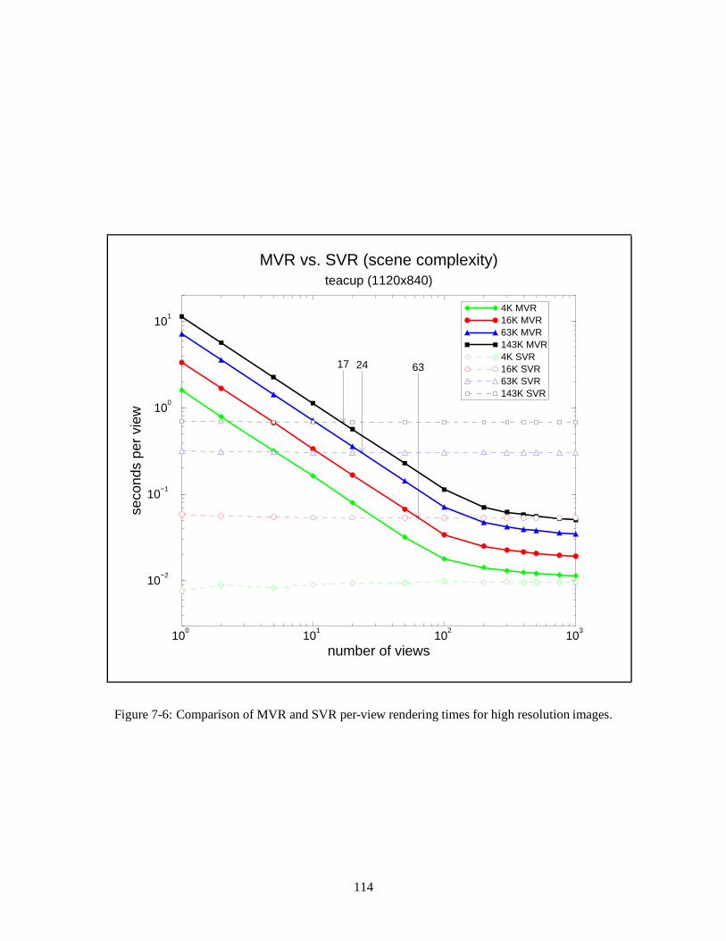
100
101
102
103
number of views
10−2
10−1
100
101
seco
nds
per
view
MVR vs. SVR (scene complexity)teacup (1120x840)
4K MVR16K MVR63K MVR143K MVR4K SVR16K SVR63K SVR143K SVR
17 24 63
Figure 7-6: Comparison of MVR and SVR per-view rendering times for high resolution images.
114

100
101
102
103
number of views
10−3
10−2
10−1
100
101
seco
nds
per
view
MVR vs. SVR (scene complexity)teacup (160x140)
4K MVR16K MVR63K MVR143K MVR4K SVR16K SVR63K SVR143K SVR
4 5 11 38
Figure 7-7: Comparison of MVR and SVR per-view rendering times for low resolution images.
1000 views. Since both MVR and SVR are pixel-fill limited in this case, their costs asymptotically
approach each other. For all other polygon databases, the break-even point has shifted by a factor
of about 1.75 compared to the 640�480 resolution image, the ratio of the scale-up in pixel size.
For the lowest resolution images, MVR is significantly faster than SVR. Figure 7-7 shows
these results. At a pixel resolution of 160�140, MVR generates a relatively small number of PSTs
to render, while SVR must render all of the polygons of the database, each with very few pixels.
The tradeoffs are such that for the highest polygon count database, only four views are required to
reach the break-even point. For the same database, MVR is more than 100 times faster than SVR
for rendering 1000 views.
115

100
101
102
103
number of views
10−3
10−2
10−1
100
101
seco
nds
per
view
MVR vs. SVR (resolution)ferio (136858 triangles)
MVR 1120x840MVR 640x480MVR 160x120SVR (all res’ns)
2.3 7 10.3
Figure 7-8: Comparison of MVR and SVR rendering times as a function of image resolution.
7.3.2 Image size dependencies
The next set of experiments summaries the relative efficiency of MVR in comparison to SVR over
a range of resolutions for a database of a fixed number of polygons. Both MVR and SVR renderers
were set up to render views at three resolutions: 160�120, 640�480, and 1120�840. The 137K
polygon Ferio database was used as a test object, and the renderings were performed on the same
Indigo2 Maximum Impact system.
In the single viewpoint renderer, the resolution of the images made no significant difference in
the per-view rendering time: each view took about one second to generate at each of the three image
resolutions. As a result, only one SVR line is indicated on the result graph, shown in Figure 7-8.
The multiple viewpoint algorithm is, as previously shown, affected by changes in pixel resolution.
The break-even points for the three image sizes are noted on the graph, ranging from 2.3 for the
116

0 10x10 50x50 100x100number of views (per dimension)
0
250
500
750
tota
l ren
derin
g tim
e (s
econ
ds)
MVR (full parallax)teacup (640x480 view res.)
4K tris16K tris63K tris100K tris143K tris
Figure 7-9: Performance of MVR using a full parallax rendering algorithm.
smallest to 10.3 for the largest. Otherwise, these tests corroborate the results of the previous set of
experiments performed on the Onyx.
7.4 Full parallax MVR
The final test shows the performance of MVR when used to render a full parallax, two-dimensional
matrix of views. The 2D matrix is rendered by decomposing it into a set of one-dimensional hori-
zontal parallax only sequences, which are rendered sequentially. For these experiments, the teacup
database at different tessellation levels were rendered on the SGI Onyx system. The image pixel
size of the output images was set to 640�480.
Figure 7-9 shows that for full parallax grids up to one hundred views on each side, the cost
of rendering grows linearly as a function of grid size, not grid area. The cost of SVR, in contrast,
would increase quadratically as the grid grows. This difference in growth occurs because , MVR
117

is vertex limited when rendering less than 100 views at this image resolution and on this hardware.
Therefore, the cost of rendering an HPO sequence of 5, 10, 50, or 100 views is the same. The linear
growth of MVR is a direct result of more HPO sequences being rendered: the coherence of vertical
perspectives is used to only a minor extent in this simple full parallax rendering scheme.
7.5 Rendering accuracy
Ideally, MVR and SVR algorithms would produce pixel-identical renderings of the same scene. In
practice, such accuracy is neither likely nor necessary. Even different implementations of the same
graphics library by different software vendors can produce slightly different renditions of geometry
and shading. On the other hand, large or inherent errors in either geometry or shading defy the basic
principle of equivalent algorithms. This section presents a direct comparison between the output of
the MVR and SVR prototype implementation.
Figure 7-10 shows four images taken from two horizontal image sequences of sixteen images
each. The sequence shown on the left was rendered with SVR, the one on the right was rendered
with MVR. The middle column shows the absolute value of the difference between the two images,
with inverted contrast to reproduce better in print. Figure 7-11 is an enlarged image of the area
outlined by the rectangle in Figure 7-10. In the difference image, two types of errors are visible.
The light gray areas represent shading artifacts. In general, these errors are less than five percent
of the total dynamic range of the image. Shading differences result from the different methods in
linear interpolation across triangles as well as from PST shading errors.
Larger but less frequent errors are the result of misaligned geometry. Differences due to this
problem show up on the lip and at the edge of the cup. Throughout the sixteen image sequence, this
geometric error resulted in artifacts never more than one pixel wide along an edge, and remained
consistentlyattached to that edge. The most likely cause of error is a small mismatch in the geometry
used by the MVR and SVR pipelines, yielding two images of slightlydifferent sizes. The differences
in shading and geometry are so minor in this sequence that a stereoscopic image pair of one MVR
and one SVR image can be viewed in a stereoscope without any artifacts being visible.
7.6 When to use MVR
The results of this chapter clearly indicate that MVR improves rendering performance for non-
pathological scenes over a moderate number of viewpoints. In some cases, though, a very large
number of views must be rendered before the average efficiency of MVR exceeds that of SVR. Even
worse, a few types of scenes with objects that exhibit high spatial coherence may take significantly
longer to render using MVR.
118

Figure 7-10: A comparison of the output of SVR and MVR. Both sets of four images were takenfrom a larger set of sixteen. On the left, an image sequence rendered using SVR. On the right, anMVR-rendered sequence. In the middle, a difference image consists of pixels values of one minusthe absolute value of the difference between the images. The rectangle shows the area enlarged inFigure 7-11.
119

Figure 7-11: An enlargement of the difference image in Figure 7-10. The light gray areas are shad-ing errors. The darker broken lines at the lip and edge of the cup are due to geometry misregistration.
120
For example, a scene composed of a collection of slender, nearly vertical polygons would be
decomposed by the MVR algorithm into many polygon slices. These slices break up the spatial co-
herence of the original scene. Rendering the slices as PSTs instead of of drawing the long polygons
themselves might significantly increase the cost of MVR rendering.
The basic rule of thumb for deciding if a scene is a good candidate for rendering using MVR
is as follows:
If the average pixel height of a polygon in a final output view is smaller than the number
of perspective views to be rendered in the image sequence, then MVR will probably
perform the same or better than SVR.
This rule is a simple comparison between the relative amounts of spatial and temporal coherence
in a scene. One important specific case is the generation of stereoscopic image pairs for two-view
display devices. MVR is usually not well suited to this computer graphics rendering task. Two
views is not enough image samples to extract significant performance gains from the coherence in
all but the most complex scenes. In general, MVR is most useful only for longer image sequences.
Other application-related factors, such as the use of texture mapping or the need for output data in
EPI-major or viewpoint-major order, should also be considered.
121
Chapter 8
Relationship to other work
The multiple viewpoint rendering algorithm described in this thesis was developed based on the
requirements of three-dimensional display devices, specifically holographic stereograms. The re-
search on this MVR algorithm dates back to work in volume rendering for holographic stereograms
done by the author in 1989. The concepts of MVR for point-cloud images such as those produced
by the dividing cubes algorithm [16] were developed in 1991. Other concepts were outgrowths
of the author’s work in optical predistortion for three-dimensional displays based on warping the
spatio-perspective image volume [32]. Even supporting ideas, such as what Bolleset. al. refers to
as epipolar plane images, were developed by the author independently based on first principles.
As a result, parts of the work contained in this thesis predate many of the related documents
from different fields included in this section. Now that the MVR algorithm has been fully described,
it is possible to compare its approach, performance, advantages and disadvantages to related work
from other fields. This chapter outlines important related research on a field-by-field basis. A few
developments such as image compression and image based rendering are related to MVR closely
enough to merit further discussion in the applications and extensions chapter that follows.
8.1 Computer generated 3D images
The first computer generated stereoscopic image pairs were created by A. Michael Noll in 1965 [55].
This work on single pairs was followed in November of the same year by a paper demonstrating
three-dimensional movies [54]. For both methods, an IBM mainframe computer generated a series
of line drawings and wrote instructions for drawing them to a magnetic tape. This tape then fed
the instructions to a film recorder, which wrote to either microfilm or 16mm movie film. Noll’s
remarkable image sequences show visualizations of a four-dimensional hypercube being turned
inside-out and a simulation of the motion of the basilar membrane of the ear in response to an
acoustic pulse. Noll’s foresighted conclusions are worth quoting: “The preceding examples indicate
122

several possible applications of computer-generated three-dimensional movies in both the sciences
and the arts....As technology progresses, increasing numbers of scientists, animators, artists and
others will use the graphic capabilities of computers coupled with devices for producing visual
output. Completely new approaches to presenting complicated concepts will become possible. The
computer generated three-dimensional movies described in this article are only a small glimpse at
what the future may bring.”
The creation of computer generated autostereoscopic displays dates back to the holographic
stereograms of King, Noll, and Berry in 1970 [41]. Until that time, computed holographic images
were created by calculating the individual fringe patterns required to diffract light from each object
point to all viewpoint directions [48]. Given the computational resources available at that time, such
a calculation for even moderately complex three-dimensional scenes was essentially intractable.
Noll’s system was used to compute a series of perspective images of a set of three-dimensional
lines, and print them on a film recorder. The images were then projected onto a diffusion screen
one by one. As each perspective image was recorded, a vertical strip of a holographic plate was
exposed. The result was a computer generated holographic stereogram, where each slit displayed
the appearance of a single viewpoint. In contrast to the large amount of computational time required
to compute a hologram fringe by fringe, Kinget. al.’s holographic stereogram required only 23
seconds of computer time to generate 193 perspective images.
8.2 Holographic image predistortion
The improvements in holographic display technology throughout the 1970’s and early 1980’s were
not accompanied by significant corresponding advances in stereoscopic image generation tech-
niques. The most significant advancements in image generation came in the field of image pre-
distortion, which uses computer graphics or image processing techniques to compensate for optical
distortions introduced by the display. Molteni performed such precompensation in hisStar Wars
holographic stereogram [53].
More analytic predistortion algorithms were developed by Holzbach [34] and Teitel [68] to
correct for the more extreme distortions found in the Alcove hemicylindrical holographic stere-
ogram. Holzbach’s technique consisted of rendering a large number of perspective images. A two-
dimensional warp was applied to each perspective image to compensate for the Alcove’s cylindrical
shape. Then an image based rendering method was used to form a series of synthetic horizontal
foci located on the hologram plane, with one focus for each holographic aperture. Teitel’s algorithm
used a computer graphics ray tracer to compute the predistorted images directly. Neither algorithm,
however, used any aspect of image coherence to improve the performance of the rendering process.
An algorithm similar to Holzbach’s was later used by Artn Laboratories to produce computer gener-
ated images for PSCholograms, a parallax barrier display technology [58][52]. Halle extended the
123

post-processing predistortion algorithms to wide angle of view holographic stereograms [33] and
full color displays [42].
8.3 Computer vision
Computer vision algorithms, and more specifically shape inference algorithms, use two-dimensional
information from some number of sensors to deduce the three-dimensional shape of an object. There
is widespread research on shape from shading and shape from a limited number of viewpoints, but
all such algorithms are prone to noise and image ambiguity when analyzing realistic scenes. Several
researchers concentrated on analyzing data from image sequences, as described by Aggarwal and
Nandhakumar [5]. In 1987, Bolles, Baker, and Marimont presented work on epipolar-plane image
analysis [12]. Their simplest camera geometry consists of a camera moving on a linear track in
front of a scene. The camera’s optical axis remains perpendicular to the camera track throughout
all camera positions. The camera captures views at regularly spaced intervals. Using this camera
geometry, objects translate strictly horizontally in the resulting camera images, at a rate inversely
proportional to the object’s distance from the camera. An epipolar line is a horizontal sample
through a single perspective image. An epipolar plane image is the collection of images of a single
epipolar line as seen in all captured perspective images.
Bolleset. al.perform scene analysis by looking for tracks made by object details in an epipolar-
plane image. For the camera geometry described above, unoccluded objects trace a linear path
with a slope related to the object’s depth. A computer vision algorithm can detect these paths and
convert them back to a three-dimensional location. If many input camera views are used to form the
epipolar-plane image volume, noise in any one image contributes little to the final depth analysis.
As a result, a large number of input views leads to improved noise immunity. Trajectories of objects
close to the camera occlude those further away. The paper further describes perspective image
volumes composed of images captured by a camera moving along a curved track could be warped
into the same form as the simple camera geometry described above.
Takahashi, Honda, Yamaguchi, Ohyama, and Iwata used epipolar-plane image analysis to gen-
erate intermediate views from a smaller number of photographically acquired images for use in
holographic stereograms [66]. Although they claim good results for the process, they do not give
efficiency results nor publish any solutions to the correspondence problem in low-detail areas.
8.4 Stereoscopic image compression
Related to computer vision approaches to image understanding and interpolation are stereo image
compression algorithms. Stereo image compression seeks to use the similarity between images in
a stereoscopic image sequence to fit the data representing those images into a smaller transmission
124

channel. Finding ways to compress stereo images amounts to solving a relaxed version of the
correspondence problem. If exact correspondences between details in the image sequence could be
found, these details could be encoded together with great efficiency. However, good compression
ratios may be obtained using approximate rather than exact matches. Image characteristics such as
shot noise, hidden and revealed areas, and viewpoint dependent lighting effects that hinder robust
solutions to the correspondence problem can still be compressed, although perhaps by sending more
image information.
Lukacs proposed using predictive coding for both stereo pairs and stereoscopic image se-
quences for use in autostereoscopic displays in 1986 [49]. His work does not seem to go beyond
simple block disparity matching, however. Most other work in the field is concerned with compres-
sion of single stereo pairs or stereo pair movie sequences. Perkins examined two different methods
of compressing stereo image pairs in 1992, one coding the two channels separately and the other
coding them together. Tamtaoui and Labit used motion compensation to compress stereo movies
[67]. Sethuraman, Siegel, and Jordan used a hierarchical disparity estimator to compress stereo
pairs and stereo sequences [59]. For image sequences, they used MPEG compatible compression
for the left views, and estimated the right views using the left images. In 1995, they extended their
research to include a region-based disparity estimator with variable-sized blocks, improving both
compression ratios and image quality [60]. Althoughaccurate solution of the correspondence prob-
lem is not necessary for any of these algorithms, they all suffer from the need to perform an image
analysis and correspondence search to find correlated image regions. No explicit three-dimensional
information about the scene is available to identify corresponding regions without search.
Only a small amount of work has been done in the area of human sensitivity to sampling
and compression artifacts in stereoscopic images. Dinstein, Kim, Tselgov, and Henik blurred and
compressed one or both stereo images in a pair and evaluated performance of a depth-dependent
task [21]. Their main result was that performance was relatively unaffected by blurring one of the
two images in a stereo pair. Halle described the sampling limitations of autostereoscopic displays
required to avoid aliasing artifacts manifested by vertical stripe artifacts [31]. St. Hilaire also
examined issues of sampling in holographic stereograms [61].
8.5 Computer graphics
8.5.1 Coherence
As holographic display technology advanced, significant inroads were being made in the field of
computer graphics. Improvements in the efficiency of computer graphics algorithms came from ex-
ploiting coherence in scene databases (object space coherence) or images (image space coherence).
Significant reductions in the time required to generate a single frame were made by using this co-
125

herence. Although motivated by the desire for computer generated films, however, little progress
was made in using the frame coherence in image sequences. Sutherland, Sproull, and Schumacker
created a taxonomy of coherence types in 1974 [65]. In their review paper, they note that while a
variety of algorithms exploit image coherence within a single frame, “it is really hard to make much
use of object and frame coherence, so perhaps it is not surprising that not much has been made.”
This quote is as much a commentary on the limited computer graphics hardware of the day and, as
a result, the impracticality of generating computer generated movies of any length than it is a state-
ment about the difficulty of exploiting frame coherence. It does show, however, that frame coherent
algorithms are a relatively new development in computer graphics.
The use of frame coherence became more viable, and more necessary, with the advent of ray-
tracing computer graphics algorithms [75]. Badt first described the use of temporal coherence in
ray tracing in 1988 with two algorithms, one using object-space coherence, the other image-space
coherence [6]. Badt’s work was followed by improved algorithms from Chapman, Calvert, and
Dill [14], and Glassner [27]. Each of these algorithms have significant drawbacks, however. Some
support only object motion, not viewpoint motion. Others place significant restrictions on image
light models. Groeller and Purgathofer [29] produced a less limited algorithm using manipulation
of a hierarchical space partitioning tree, with computational gains for simple scenes up to a factor
of two. This algorithm, like the ones before it, are tied strongly to the ray-tracing image generation
paradigm, and thus are impractical for rapid image generation. A more thorough characterization
of frame coherent algorithms can be found in a 1990 taxonomy by Tost and Brunet [70].
8.5.2 Stereo image generation
Adelson and Hodges have presented a series of papers related to the generation of stereoscopic im-
age pairs by taking advantage of perspective coherence in various different ways. In 1990, Ezell
and Hodges used Badt’s second algorithm to generate stereoscopic image pairs [24]. Adelson and
Hodges further refined the reprojection algorithm [4]. Adelson, Bentley, Chong, Hodges, and Wino-
grad demonstrated modest computational savings using a scanline-based stereoscopic rendering al-
gorithm in 1991 [3]. Collectively, these algorithms appear to be the first to use characteristics of
stereoscopic images to simplify rendering. They computed only single pairs of images, however.
8.5.3 Hybrid approaches
Zeghers, Bouatouch, Maisel, and Bouville presented an algorithm in 1993 [78] that uses motion
compensated interpolation to produce a series of intermediate frames in an image sequence using
pixel and motion field information from two fully-computed frames (known as base images). This
algorithm has the advantage that the image interpolation is independent of the actual rendering
algorithm used to compute the two base images. Its primary disadvantages are that the motion field
126

of the images must be computed, and that the interpolation of image data is done in image space,
reducing image quality in areas of fine detail.
Chen and Williams [15] also use computer graphics information to guide the viewpoint inter-
polation of synthetic scenes. Their algorithm uses the known camera geometries that render two
images and the depth buffers associated with those images to build an image-space morph map.
The map describes the corresponding points in the two images that should be interpolated to find
the position of image detail as seen from an intermediate viewpoint. Chen and Williams point out
the usefulness of this type of interpolation for costly operations such as shadow and motion blur
rendering. They discuss the significance of a view interpolation algorithm that can be performed at
a rate independent of scene complexity. Their algorithm includes methods for reducing problems
of “overlaps” (areas of the image where two different surfaces occlude each other as seen from the
intermediate viewpoint) and “holes” (places in the final image where no image data is known).
These problems, though, can only be minimized, not eliminated in the general scase scenes.
The algorithm also cannot handle anti-aliased input images because of the primitive model of three-
dimensionality supported by the image-space depth-buffer. Specular highlights and other view-
dependent lighting phenomena are not interpolated correctly because they move differently than
the object described by the depth-buffer. Some error in image interpolation of specular highlights
may be tolerable, but a high quality rendition of a scene with such highlights would require many
original input images.
In contrast, MVR uses the original scene data, not an image space depth buffer, as its model of
the scene for interpolation. Using this data permits much a more accurate geometric interpolation
to occur during the rendering process that is compatible with anti-aliasing and view-dependent
shading. On the other hand, the rendering cost of MVR is dependent on scene complexity unlike an
image space algorithm.
The Zegherset. al. and Chen and Williams’ algorithms are perhaps most significant because
they bridge the gap between the computer graphics rendering process and image processing al-
gorithms such as motion compensated interpolation. Wallach, Kunapalli, and Cohen published a
solution to a complementary problem in 1994 [73]: they use a polygonal rendering algorithm to
produce an image of the object motion field. This information is then used as a hint for an MPEG
image sequence compressor. The standard MPEG compression algorithm encodes moving object in
an image sequence by searching for similar blocks from frame to frame in the sequence. The mo-
tion field hint directs the MPEG compressor to look for a matching block in a particular direction.
Wallachet. al.’s major contribution is the computation of the motion field directly from a polygonal
database.
These hybrid algorithms demonstrate how computer vision, computer graphics, and image
processing techniques can be merged together in mutually beneficial ways. Other recent such hy-
brid computer graphics algorithms include work by Levoy [45] and McMillan and Bishop [51].
127

McMillan and Bishop present work most relevant to multi-perspective imaging by warping parts of
two-dimensional images to simulate viewing from arbitrary viewpoints. The algorithm is limited by
the ambiguity of the two-dimensional image input data: the three-dimensional position of objects
is not known and must be inferred. In this case, the computer graphics algorithm is limited by the
difficulty in solving the correspondence problem in computer vision.
Some of McMillan and Bishop’s concepts have been extended into a growing field of research
tentatively given the termimage based rendering. Levoy and Hanrihan [46] and Gortleret. al.
[28] have presented work that uses a sampling of image data from disparate viewpoints to produce
new images from arbitrary viewpoints. Levoy and Hanrihan’s work uses images taken using a PRS
camera geometry, while Gortler et. al. use a regularization method to process data sampled from
from an irregular set of camera locations. Image based rendering algorithms of the type described
by Levoy and Hanrihan are equivalent to those used for holographic predistortion, except that one
image is extracted rather than a sequence. The relationship between image based rendering and
MVR will be discussed more fully in the applications and extensions chapter.
128

Chapter 9
Applications and extensions
This chapter discusses uses for multiple viewpoint rendering and extends the ideas to new areas.
The foremost and most straightforward application of MVR is the generation of images for three-
dimensional parallax displays. MVR can, for example, be used as an input stage for image predis-
tortion algorithms and other image based rendering techniques. Techniques used in MVR can be
applied to camera geometries other than the PRS camera. While the previous sections described
polygon rendering, other primitives can also be rendered within an MVR framework. Depending
on the application, MVR can be parallelized to maximize the speed of rendering. Finally, MVR
can be used as a compression algorithm, splitting the renderer into two pieces across a transmission
line. The diverse set of applications described here are only an overview of possible uses for MVR.
While these examples focus mostly on HPO imaging, many of the techniques are also applicable to
full parallax imaging as well.
9.1 Application to three-dimensional displays
The PRS camera geometry was developed in Chapter 3 specifically to match the requirements of
the common parallax display model. Generating image data for a particular parallax display first
requires fitting the display’s geometric and optical characteristics to the parameters of the common
model. These parameters include the number of required perspective samples, the density of each
camera image, and the size and location of the camera and image planes.
These camera parameters are used along with the scene description as input to the MVR al-
gorithm. The rendering process produces image data that conforms to the specified geometry. For
display types that closely match the common display model, the information can be used directly to
drive the recording or display device. In most cases some amount of data reformatting is required.
For instance, some displays may need image data in viewpoint-major format, while others might be
able to use EPI-major format directly. Similarly, one type of display might use all the perspective
129

information for one direl at once, while another might display the light leaving all direls on a scan-
line from one direction at a time. Adapting the ordering of the stream of image information to the
needs of the particular display is a relatively simple reshuffling operation that can be done either
during rendering or as a post-processing step.
9.1.1 Predistortion
In some cases, the optical characteristics of a display make it an imperfect match for the common
parallax display model. For example, optical aberration may warp the shape of the display’s aperture
plane into something no longer planar, or move it away from the view zone. Distortions of this type
may be wavelength dependent in the case of diffractive optics, sending red, green, and blue light to
different positions in space. Without modification, image data rendered by any method will produce
a spatial image that appears distorted, moves incorrectly, or has color fringing.
In the case of such distortions, the output of MVR can often be warped to form a new spatio-
perspective image volume that compensates for the display’s optical aberrations. For HPO images,
the warp is often restricted to the horizontal direction, so EPIs can be warped at the time at which
they are produced. The warping process can also include data ordering required by a given display
type.
9.1.2 Holographic video
Holographic video display is a good example of an application to which the characteristics of MVR
are well-matched. The first holographic video, or electro-holographic, display systems were de-
veloped at the MIT Media Laboratory [62]. The details of the display technology are beyond this
paper’s scope; only the essential characteristics of the system will be described here. A holographic
video display uses an electrically-driven diffractive element such as an acousto-optic light modulator
to bend and focus light from a source beam. The frequency components of the incoming electrical
signal determine in which directions light is diffracted. A superposition of different frequencies can
result in a complex output wavefront. The optical system of a holographic video device produces
an image of the diffractive modulator that spans the image plane of the display. An appropriate
diffraction pattern varying across the image plane results in an output wavefront that focuses light
to form a three-dimensional image.
Techniques borrowed from holographic stereograms, such as HPO imaging and spatial dis-
cretization, are used to reduce the information requirements of holographic video. In an HPO imag-
ing system, each horizontal line of the output display can be considered independently. Each such
scanline is broken into discrete elements, where each element can diffract light into a discrete set
130

of directions. These elements are direls of the display. The electrical signal applied to the display
controls the relative intensity of the light diffracted in the each of the different discrete directions by
each direl.
Figure 9-1 shows a summary of the process of rendering for holographic video. The rendering
process must calculate the appearance of each direl as seen from each direction. If all direls have
the same set of directions, the appearance of all direls as seen from one direction can be found using
a computer graphics camera placed at infinity looking at the image plane, with each pixel of the
resulting image corresponding to a direl. An MVR camera is used to render the camera views that
correspond to all the ray directions simultaneously.
The data from the MVR camera forms an EPI volume. In each EPI in the volume, the appear-
ance of each direl as seen from all views is stored as columns of pixels. The pixel intensity values
from each such column describe the piecewise intensity of the appropriate direl’s wavefront. The
intensity values are used to modulate a set of precalculated waveforms that diffract light in specific
directions. The sum of these intensity-weighted waveforms is the modulation function for the direl.
The signals for all the direls on a scanline are abutted and used to drive the light modulator.
Other dynamic parallax displays, such as lenticular sheets places over CRTs or other image
modulators, could use a similar MVR-based rendering system to produce EPI-major data for rapid
display.
9.2 Image based rendering
Image based rendering is recent paradigm of computer graphics that manipulates image data
instead of explicit geometry to form new images. Both light field rendering [46] and the lumigraph
[28] use large amounts of image data and information about camera locations to render arbitrary
views of a three-dimensional scene. This work is conceptually and algorithmically similar to holo-
graphic image predistortion methods [33]. Each of these techniques work by resampling known
data about the plenoptic function around an object to form new viewpoints. In effect, they imple-
ment computationally what a parallax display does optically: convert a dense sampling of image
information into a new viewpoint or set of viewpoints.
Just as MVR is an efficient image generation technique for three-dimensional displays, it can
also be used to generate input image data for image based rendering systems. The regular grid of
camera viewpoints implemented by MVR with the PRS camera geometry can be used directly by
the light field rendering algorithm. MVR serves as a geometry to light field converter, from which
the light field resampling algorithm can extract arbitrary views.
131

referencebeam
piecewise-modulatedwavefront
diffractivelight modulator
Σ
p
x
image plane (enlarged)
lines of sight from distant cameras through each pixel on the image plane
one pixel
a strip of datafrom the epipolar plane image captured with thegeometry above, showing the appearance of one of the pixels seen from all viewpoints
pixel intensities modulate the elements of a bank of waveforms, each of which diffracts light in one direction
weighted sum of waveforms
Figure 9-1: MVR rendering for an HPO holographic video display.
132

scenegeometry perspective
image sequence
light fieldrendering
MVR
image predistortion
predistortedimage sequence
arbitraryperspective
Figure 9-2: MVR provides conversion from geometry to image data that image based renderingtechniques can use to produce arbitrary views or view sequences.
133

9.3 Application to other rendering primitives
9.3.1 PST strips and vertex sharing
Vertex sharing, another common geometry compression technique, can be applied to MVR com-
pression to reduce geometric redundancy. Vertex sharing is used in triangle strips and meshes in
SVR to increase the pixel-to-vertex ratio. SimilarPST stripscan be formed by the MVR renderer
either during slicing or just before PST rendering to further improve the� of MVR. Finding PST
strips in the polygon slice database is a one-dimensional search problem, which makes finding PST
strips easier than finding triangle strips.
9.3.2 Point cloud rendering
The database of a point cloud scene consists of a collection of points, each represented by a posi-
tion, a color, and a surface orientation vector. Data of this type is produced by the dividing cubes
algorithm [16]. Point primitives are easier to render than polygons because of their simplicity. Point
databases are also easier to edit because each primitive never require subdivision. For sparse data,
an irregular grid of point cloud data may be more efficient for storage than a mostly-empty data
volume on a regular grid.
Rendering oriented point primitives is MVR is also simpler than rendering polygons. Each
point forms a line through an EPI. View independent shading is linearly interpolated from one end
of the line to the other. While the point primitives do not need to be sliced, they do need to be sorted
into scanlines after transformation.
Holes in the surface due to insufficient density of the point cloud are an artifact that occurs with
point cloud images rendered using any method. The sampling density is determined in world space
based on the approximate resolution of the final output display. Extreme transformations, such as
the shearing that occurs near the ends of the MVR view track, are more likely to produce these
holes. Hole artifacts can be reduced or eliminating in MVR by scaling the primitives horizontally
to fill more space at the extreme perspectives. Scaling is based on the dot product of the view vector
with the horizontal component of the primitive’s surface normal. Where the absolute value of the
dot product is close to unity, no scaling is required. Where it is close to zero, the track of the line
through EPI space must broaden most rapidly towards the extreme perspectives. Although current
graphics hardware does not support lines of width that varies along their length, the effect can be
approximated by breaking the line into discrete segments of constant width.
134
9.3.3 Volume rendering
The very first MVR-like algorithm developed in the course of this research, and the inspiration for
the polygon rendering algorithms previously described, was a volume rendering algorithm. Vol-
ume rendering uses a regular grid of data to describe a scene [22]. Shading operations turn image
data into per-voxel color and opacity values based on light models, edge strength, and user-defined
editing. MVR can be used to render multiple viewpoints of a data volume. For simplicity, this
algorithm assumes that the color and opacity information can be reformatted to form a volume with
planes parallel to the MVR camera plane, and that only view independent lighting calculations are
used in the volume lighting calculations. Each depth plane can be considered a complex filter acting
on all the planes behind it. To compute the appearance of the volume from a single direction, the
“over” image compositing operator [23] is applied pixel by pixel toeach depth plane from back to
front.
The MVR volume renderer can composites EPI images of each depth slice. Figure 9-3 shows
the basic pipeline for MVR volume rendering. A set of EPIs is generated for each horizontal plane
through the data volume, one EPI per data scanline. The EPI for each data scanline is just that
scanline swept through perspective space with a slope defined by the distance between the scanline
and the image plane. Each scanline has a constant slope. The EPIs for all the data scanlines can
be composited to form a final EPI. This EPI holds the appearance of the horizontal slice of the data
volume seen from all locations on the view track.
9.4 Compression for transmission and display
Three-dimensional television has been the dream of the public and scientists alike dating back at
least as far as the work of Herbert Ives in the 1930’s. The major stumbling block to any system for
transmission of 3D is the large bandwidth of the information. Using HPO displays and limiting the
number of views to be transmitted reduces these costs at the expense of some image fidelity. Even
with these approaches, though, unencoded transmission of the three-dimensional image data is still
prohibitive, both from information content and business standpoints. The long-term commercial
revenue for one “four-view” 3D television station is most likely eclipsed by that of four conventional
monocular stations.
The advent of digital television brings with it the possibility of using perspective coherence
to reduce the channel requirements of the highly-redundant 3D views. Compression methods such
as MPEG, which use image based prediction along with other coding techniques, work on image
data from a sequence to reduce the amount of information that needs to be transmitted. At the other
end of the algorithmic spectrum, model-based or computer graphics methods send an explicit three-
dimensional scene description to the receiver and ask that the decoding system turn it into image
135
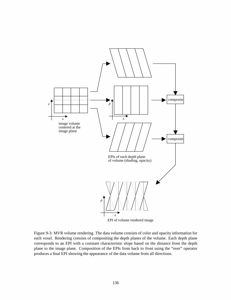
composite
composite
image volumecentered at the image plane
EPIs of each depth planeof volume (shading, opacity)
EPI of volume rendered image
z
x
p
x
p
x
Figure 9-3: MVR volume rendering. The data volume consists of color and opacity information foreach voxel. Rendering consists of compositing the depth planes of the volume. Each depth planecorresponds to an EPI with a constant characteristic slope based on the distance from the depthplane to the image plane. Composition of the EPIs from back to front using the “over” operatorproduces a final EPI showing the appearance of the data volume from all directions.
136

scenedatabase
MVRper-vertexcalculationand slicing
visibility rendering
view-independent rendering
view-dependent rendering
imagedifference
transmitter
receiver
geometrydecompression
geometrycompression
for each scanline
culled slice database
polygonslice database image
compression
slice database view-independent
rendering
imagesum
imagedecompression
EPI
transmission channel
scanlinedisplay
Figure 9-4: This block diagram shows a system for the transmission of view-count independentthree-dimensional images, based on a hybrid geometry and image data stream.
data. The object description may be compact compared to the amount of image information it
represents, but the receiver must be powerful enough to perform the task of decoding and rendering
it.
MVR can be used as a basis for a compression and transmission technique that shares attributes
of both the image-based and the model-based algorithms. A schematic of the system described here
is pictured in Figure 9-4. The MVR technique, like the geometric approach, begins with an explicit
scene description of an object. The MVR encoder performs all of the view independent calculations
of the MVR pipeline, including transformation, view independent lighting, scanline intersection,
and per-slice texture extraction. The polygon slice database formed by slice intersection is the
basis of the information to be transmitted to the receiver. The elements of the slice database are
still geometric and have continuous representations. However, the transmitter has done much of
the work of scan conversion and lighting, and the vertical resolution of the database is fixed to the
number of scanlines of the output display.
137

For the receiver, rendering the slice database is much easier than rendering the original scene
geometry. Rendering consists of converting the continuous slice database into EPIs for each scan-
line. The number of views to be rendered is decided by the receiver, not the transmitter: different
quality displays can all render the same slice database. The polygon slices in the slice table are
stored in scanline order, so all of the slice information for a particular EPI is transmitted together.
For a three-dimensional display device that scans out the image data from one EPI at a time, poly-
gon slices can be rendered into the current EPI and discarded without requiring additional storage.
One-dimensional texture vectors for each slice can also be transmitted, used, and deleted in this
way. Texture mapping and other view independent shading can be efficiently implemented using
image resampling and warping hardware commonly used for video effects.
Polygon slice data is amenable to compression for efficient transmission. Scene heuristics
estimate the coherence used to guide this compression. For instance, the polygons that compose
many scenes are located close to the image plane, are oriented approximately parallel to it, and
have a fairly constant horizontal extent. In other words, an object can be approximated to a first
order as a planar object on the image plane with a fixed number of polygons. The polygon slices
for such an object would correspond to PSTs with almost vertical i-edges and with relatively short
p-edges. This kind of geometry can be compressed by converting the slice coordinates to a fixed-
point representation, difference encoding the slice endpoints, and entropy encoding the results to
efficiently encode slices of the most typical size. Other forms of scene geometry compression such
as those proposed by Deering [19] can also be used. In addition, thez coordinates of each slice can
be disguarded by the transmitter because depth information is implicitly encoded by the difference
of x coordinates.
For complicated scenes, many polygons in the original database may not be visible anywhere
within the range of viewpoints of the MVR camera. The slices that result from these polygons do
not affect the appearance of the receiver’s image and can be culled before transmission. To perform
this culling, the MVR encoder pre-renders each EPI, but shades each PST using a constant and
unique color, without anti-aliasing. This type if rendering is calledvisibility rendering. The color
acts as a label for each pixel to indicate which polygon slice produced it. Once the EPI is rendered,
the transmitter sends only the slices that were labeled by at least on pixel in the EPI.
View dependent shading can be handled in two ways. First, shading can be modeled geomet-
rically just as in the MVR rendering algorithm described previously. If this approach is chosen,
the receiver must have extra information about the scene, such as light sources and material prop-
erties, and must perform more rendering calculations. Alternatively, the transmitter can encode the
difference between a high quality image with view dependent shading and the lower quality view
independent image and send it as a compressed error signal. The receiver adds the error signal to the
output of its view independent renderer to recreate the higher quality image. This idea is similar to
Levoy’s geometry assisted compression [45]. Most compression techniques include this kind of er-
138

ror image to make up for shortcomings of the compression model, so the view dependent difference
image fits well into this model.
9.5 Opportunities for parallelization
The MVR algorithm is well-suited for computational parallelization. Opportunities exist for both
data parallel (simultaneous processing of different parts of the data set) and process parallel (pipelin-
ing a series of computations performed on one piece of data) operations. Efficient parallelization
depends on access to the entire scene database at once; the “stream of polygons” model common
in immediate-mode rendering hardware systems is not compatible with MVR rendering because of
the EPI-major ordering of the rendering process.
MVR’s per-sequence processing stage is similar to SVR in being the most difficult to parallelize
efficiently. Per-vertex transformation and shading operations on scene polygons can be readily
distributed over a set of processors since these operations require a fixed amount of computation.
Scanline intersection and polygon slice generation, however, have a computation time dependent
on the size of the polygon being processed. Since the size of the transformed polygons is not
known when polygons are assigned to processors, some processors assigned only small polygons
may sit idle while processors with large polygons continue to run. In addition, the slice table is a
writable global data structure that must be accessed by all processors to record the result of their
slicing operations. Slice table entries must be locked before writing to avoid data corruption; this
locking may lead to resource contention and processor waiting. For full parallax rendering, different
horizontal image subsequences can be processed in parallel when memory for such an operation is
available.
Once the slice table is completed, however, the remaining stages of MVR can be both parti-
tioned and pipelined. Each slice table entry describes all of the scene geometry that contributes to
the corresponding EPI completely. Each EPI, then, can be processed independently and in parallel.
The time required to render one EPI is dependent on the number of slices that intersect the corre-
sponding scanline and the pixel area of the PSTs that must be rasterized. Both of these values can
be used when scheduling resources for each EPI: the number of slices is known, and the area of the
PSTs can be estimated based on the width and orientation of each slice.
In SVR, polygon rasterization is difficult to parallelize because a single polygon can be large
or small, nearly isotropic or very wide or tall. Parallel rasterization usually assigns parts of the
screen to different processors, so the size and shape of polygons directly affects the efficiency of
scheduling. PSTs, on the other hand, have a more regular shape than typical polygons. For instance,
PSTs cross most or all scanlines of the EPI. Resource allocation based on heuristics of the primitives
are more likely to be correct, and efficiency of rendering can be maximized as a result.
139

When MVR serves an the rendering stage of a larger imaging or display pipeline, the data from
each EPI can be processed in pipeline fashion by each subsequent stage as it is produced by the
renderer. A discussion of this process was included in the section on the implementation of the
MVR output stage. When one of the stages of display is a scanning display device with no image
storage buffer, great care must be taken when scheduling the rendering process to assure that image
data is always available to the display device when it needs it. Image buffering can be used to
smooth out variations in the rate at which rendered image data is made available. Since storing a
complete copy of the last-rendered EPI volume (analogous to double-buffering in SVR) would be
very expensive in terms of memory requirements, partial buffering of a smaller section of the image
can be used as a compromise.
9.6 Other camera geometries
Not only is the PRS camera geometry designed to match the geometry of planar parallax displays;
it also happens to be the geometry to which MVR techniques are best suited. Two properties in
particular are very convenient. First, the regular spacing of the camera array produces linear features
that can be easily represented and rasterized. Second, the restrictions on camera alignment force
apparent object motion to be in the same axis as camera motion. The image of each object detail in
the spatio-perspective volume is restricted to an EPI, so only a small, regular subset of the volume
needs to be accessed at any one time. This property of good locality of reference is important
computationally because the spatio-perspective image volume can be very large.
While the PRS camera geometry may be the most straightforward to use with MVR, other
camera arrangements can be rendering using MVR techniques. A few camera geometries can be
created by assembling pieces of the RS camera geometry. For instance, a collection of images that
form a cylinder around an object can be constructed from a series of LRS cameras where the linear
tracks are aligned with the long axis of the cylinder. Other camera configurations can be synthesized
using image based rendering techniques to combine different parts of views generated using either
the PRS or this cylindrical camera geometry.
For certain other geometries, the path of object details through the spatio-perspective volume
that result from camera motion may be regular and readily rasterized. An object orbited by a camera
located at a great distance from an object produces a series of sinusoidal tracks with a magnitude
that depends on the distance from the object to the center of rotation and with a phase that is a
function of the object’s spatial orientation. The sinusoidal tracks become the i-edges of PSTs in this
geometry’s spatio-perspective volume. The PST can be rasterized by filling in the pixels that lie
between the two sinusoids.
Unfortunately, the geometry of the spatio-perspective volume becomes more complicated if
this orbiting camera moves closer to the object. The effect of perspective causes the track of object
140
points to cross from one scanline to another from view to view in a position-dependent pattern,
decreasing the locality of the memory that a rendering algorithm must rasterize. This property
might preclude the use of computer graphics hardware for accelerated rendering unless the device
can access a three-dimensional volume of display memory. Perspective also causes the shape of
tracks through the spatio-perspective volume to become more complicated: the apparent velocity
of a point changes depending on whether the point is close to or far from the camera. Depending
on the application, polynomial approximations of this distorted path could be used to simplify path
evaluation and rasterization.
A rendering system with access to large amounts of display memory and a flexible algorithm
for rasterization could be used to render images from a broader class of camera geometries as long
as the scene remains static and the camera grid is regular. This same system could be used for direct
rendering of full-parallax information as well. On the other hand, the general animation problem
of rendering a scene with arbitrary camera and object motion is much broader, more general, and
more difficult. The less regular the changes in the scene geometry are, the more calculation that
must be done to compute, shade, and rasterize the track of each object in the scene. Eliminating
these variables is exactly what made MVR so efficient for rendering images using the PRS camera
geometry. Efficient rasterization of the spatio-temporal volume that results from arbitrary animation
is sure to remain a subject of research for some time to come.
141

Chapter 10
Conclusion
In the past thirty years, computer graphics has evolved from wireframe images and stick figures to
full length feature movies and imagery visually indistinguishable from real objects. Realism, ani-
mation, and simulation of natural phenomena will continue to become better and faster as the future
unfolds. But the next step toward realism, the world of three-dimensional images, still lies ahead.
The multiple viewpoint rendering algorithm described in this thesis is one of the links between
today’s graphics techniques and the three-dimensional display devices of tomorrow.
Multiple viewpoint rendering is not designed to solve the general problem of animating objects
efficiently. It is tailored to a much smaller problem: how to generate a dense, regular sampling
of view information of a scene that can be used for three-dimensional display. By restricting its
scope in this way, MVR can harness perspective coherence to improve the efficiency of rendering
perspective image sequences. MVR uses explicit geometric information, not image data, to interpo-
late the positions of objects in intermediate views. Image generation can occur at rates one to two
orders of magnitude faster than existing rendering algorithms with higher quality output than image
interpolation techniques.
Today, MVR can be implemented using established computer graphics techniques, running
on existing software and hardware platforms, rendering commonplace geometric databases. Small
modifications to existing algorithms and hardware designs can bring even greater performance and
quality improvements. In the future, MVR will remain efficient as object databases become more
detailed because perspective coherence is for the most part independent of the size of the geometric
primitives that make up a scene.
The challenge of convenient, affordable, high fidelity three-dimensional displays remains daunt-
ing because of limitations of bandwidth and display technologies. Generating a single image will
always remains easier than generating many different ones. Because of this fact, MVR will not
replace single viewpoint rendering any more than 3D displays will obsolete flat, static images.
However, efficient image generation is now a much less significant obstacle to overcome on the way
142

to practical three-dimensional displays. As new strides in display and information technology are
made, multiple viewpoint rendering and techniques derived from it will be able to provide a wealth
of three-dimensional information for applications that require the ultimate in realism.
143

Appendix A
Glossary of terms
accumulation buffer An image buffer used in computer graphics to combine several rendered im-ages.
anti-aliasing Any of a series of methods used to bandlimit the signal of an image that is undergoingdiscrete sampling. In computer graphics,spatial anti-aliasingis used to avoid aliasing arti-facts such as moire patterns and jagged lines (“jaggies”).Temporal anti-aliasingintegratesthe appearance of a scene throughout the time between frame, perhaps introducing motionblur. Perspective anti-aliasingproperly samples the part ofspatio-perspective spacethat liesbetween discrete camera viewpoints, producing an effect similar to lens blur.
autostereoscopicPresenting a three-dimensional image without the need for glasses, helmets, orother viewer augmentation. Autostereoscopic is used to describe a class of three-dimensionaldisplays.
cache, cachingIn computer architectures, a cache is piece of fast memory used to store frequently-used information in order to reduce the cost of repeatedly retrieving it. Caching is the processof storing data in the cache. Cache strategies determine which data should be stored for lateruse.
coherence In computer graphics, an attribute or property shared by different parts of a scene. Co-herence is used to reduce the cost of rendering images.Image coherenceconsists of coherentproperties of a single viewpoint, such as large areas of constant color or possible representa-tion by large geometric primitives.Perspective coherenceis the similarity between an imagecaptured from one viewpoint and another captured from a viewpoint slightly offset from thefirst. Temporal coherenceis the image similarity of a camera image captured at one time toanother captured some time later.
full parallax An image property where a change in viewpoint in any direction produces a corre-sponding and proportional change in the relative apparent position of details in a scene, as afunction of the depth of the detail.
horizontal parallax only (HPO) An image property where only a change in viewpoint in the hor-izontal direction produces a corresponding and proportional change in the relative apparentposition of details in a scene, as a function of the depth of the detail. In the vertical direction,viewer motion results in detail motion of a fixed rate independent of scene depth.
camera plane The plane in space where the cameras of a PRS camera array are located whenimages are captured. The cameras in the plane look toward and re-center the image plane.
144

The location of the camera plane should correspond to the location of the display’s viewplane.
depth buffer A memory buffer that consists of one depth value per pixel of a rendered image.The computer graphics technique of depth buffering uses the depth buffer to perform hiddensurface removal. A pixel from a geometric primitive is rendered into the image buffer only ifits depth value indicates it is closer to the viewer than the depth value stored at that pixel inthe depth buffer. Also called aZ-buffer.
directional emitter A point in space capable of emitting directionally-varying light. The light’svariation can be in color or intensity.
direl Short for “Directional element”. A discrete element of a display capable of sending outdirectionally-varying light. In other words, direls look different when viewed from differentdirections. Direls can be used to createparallax displays.
disparity The difference in apparent position of an object detail when viewed from different twolocations. Thebinocular disparityof our two eyes provides our sense of stereoscopic depthperception.
display plane The plane in space that corresponds to the location of a flat-format parallax display.Compare toimage plane, view plane, camera plane.
egomotion Motion by the observer or by a camera capturing a scene.
epipolar plane The plane that lies between two camera viewpoints and a point in a scene. Theintersections between the epipolar plane and the image plane of the images captured from thetwo camera viewpoints are called epipolar lines.
epipolar plane image (EPI) A two-dimensional image made up of epipolar lines, in images takenfrom many cameras, that result from a shared epipolar plane. A collection of EPIs form anepipolar plane image volume, orspatio-perspective volume.
EPI-major ordering An ordering of image data in a data stream where an entire EPI is sent beforethe next one begins. For example, the first scanline from the first perspective image is sent,then the first scanline from the next perspective, and so on until the first EPI has been putonto the stream. Then the second scanline from the first image and all the other scanlines thatmake up the second EPI are sent. The process repeats until all EPIs have been sent. Compareto viewpoint-major ordering.
geometry compressionA class of methods for reducing the amount of memory required to repre-sent scene geometry.
hologram A diffractive optical or display device.
holographic image predistortion An image based rendering process by which the distortions in-troduced by holographic stereograms can be reduced or eliminated. Image processing tech-niques are used to introduce an opposite distortion to the images used to expose each holo-graphic aperture. The image distortion and the hologram’s distortion cancel each other, pro-ducing an undistorted image.
holographic stereogram A display that uses holographic medium to record discrete spatial anddirectional information, usually for the purpose of displaying a three-dimensional image.
145

holographic video An electronic device used to produce moving three-dimensional images usinga diffractive optical light modulator.
i-edge The diagonal edges of a PST that interpolate the shape of a polygon slice through interme-diate viewpoints of an image sequence. Short forinterpolated edge. See alsop-edge.
image plane The plane in space that all of the cameras of aPRS cameraarray center in their view.This plane represents the “center of interest” of the cameras, and usually falls in the middle ofthe volume being imaged. The image plane used in a computer graphics rendering for displaycorresponds to the display plane when the display device is viewed.
image based renderingA class of computer graphics algorithms that use image data about a sceneas a rendering primitive. Images or parts of images can be combined to form new viewpointsand perspectives on an object or scene. Image based rendering typically requires a largeamount of image data for manipulation. However, rendering a final image requires timeindependent of the original scene complexity.
image spaceThe discrete space in which a pixelated, two-dimensional image is represented. Com-putations performed in image space operate on the discretized two-dimensional samples ofthe image. These techniques are done with what is calledimage precision.
lenticular panoramagram An autostereoscopicdisplay technology that consists of a set of longvertical lenses molded into a plastic sheet. Image data behind each lens is visible from onlycertain angles.
light field rendering An image based renderingsystem that uses a regular grid of cameras as asource of image data.
LRS (linear-regular-shearing) camera geometryA one dimensionalPRScamera geometry wherecameras are arranged in a regular, one-dimensional array along a linear track. An LRS cameracapturesHPOdepth information.
lumigraph An image based renderingsystem that uses a set of images from cameras arranged atirregular intervals, along with calibration information, as source of image data.
MIP map A multi-resolution data structure used in computer graphics to minimize aliasing in tex-ture and reflection maps.
multiple viewpoint rendering (MVR) A class of computer graphics algorithms that compute theappearance of a scene from many locations at once. Multiple viewpoint rendering can exploitcoherence not found in a single image. Compare tosingle viewpoint rendering (SVR).
object spaceThe continuous space in which a geometric object is represented. Computations per-formed in object space operate on geometric primitives in three dimensions. Calculations aredone withobject precision.
p-edge The horizontal edges of a PST that are the projections of the polygon slice as seen from thetwo extreme viewpoints. Short forprojection edge. See alsoi-edge.
parallax The relationship between the change in an observer’s position and the change of apparentposition of an object detail that results from the viewer’s motion. Parallax is usually associ-ated with lateral viewer motion.Motion parallaxis the depth cue that results from observermotion.
146

parallax display A two-dimensional device that produces a three-dimensional image by filling avolume of space with directionally-varying light.
parallax panoramagram An autostereoscopic display technology that consists of a set of longvertical slits in an opaque barrier material. Image data behindeach slit is visible from onlycertain angles.
pixel A picture element. A pixel is a single element of a two-dimensional display. Light from apixel is scattered in many different directions. In a computer graphics system, animageis anarray of pixels whose appearance is under the direct control of data stored inimage memory.
pixel fill limited The state of a computer system where the most time-consuming step of a process-ing pipeline is performing per-pixel operations. Computers with slow access to the memoryin which pixel data is stored are prone to pixel fill limitations.
plenoptic function A mathematical description of light seen by a sensor along one line of sight, atone time, in one color or wavelength. Knowledge of the value of the plenoptic function inseveral of its dimensions is the basis of vision systems.
point cloud rendering A computer graphics method for photorealistic rendering where surfaces ofobjects are composed of small pieces of surface represented by a location, color, and surfaceorientation.
polygon A primitive used in computer graphics rendering as an element of a piecewise descriptionof an object.
polygon slice The intersection of a polygon with the scanline of a display. A polygon slice is aone-dimensional primitive in three-dimensional space used in multiple viewpoint rendering.
polygon slice track (PST) The portion of spatio-perspective space swept out by apolygon slice. APST is a primitive used in multiple viewpoint rendering: PSTs are scan-converted in order torenderEPIs.
prefetch Prefetching is a computer architecture technique that retrieves information from memorythat is likely to be needed in the near future. Prefetching can prevents relatively slow mem-ory accesses from slowing down faster computation. Strategies for prefetching require thatmemory accesses be predictable.
PRS (planar-regular-shearing) camera geometryA computer graphics camera geometry con-sisting of a two-dimensional array of regularly-spaced cameras, all facing perpendicular tothe plane upon which they are positioned, all of their optical axes parallel, and all of their upvectors aligned with the vertical axis of the camera plane. The cameras can shift their frustaso as to re-center all of their views on the image plane. A PRS camera capturesfull parallaxinformation about a scene.
PS (regular-shearing) camera geometryA class camera geometries includingPRSandLRS.
reflection mapping A computer graphics technique used to introduce non-geometric detail ontosurfaces of a geometric scene. Reflection maps approximate the surrounding environmentof an object as image data. Reflections are mapped onto surfaces by using the orientationof the surface and the location of the viewer to determine which part of the map to apply.The process of reflection mapping can usetexture mappingtechniques to perform the map
147

operation. Reflections do not appear attached to the surfaces onto which they are mapped.Reflection mapping is much less complex than more accurate reflection algorithms such asraytracing.
single viewpoint rendering (SVR) A class of computer graphics algorithms that compute the ap-pearance of a scene from a single location. Most conventional computer graphics packagesare SVR algorithms. Compare tomultiple viewpoint rendering (MVR).
spatial display A display device that produces an images that appears three-dimensional. Alsocalled a three-dimensional display.
spatio-perspective volumeA multi-dimensional mathematical representation of the relationshipbetween the location of a camera viewpoint and the apparent position of an object as seenfrom that viewpoint. One or more dimensions of the volume represent the spatial domain ofthe object, while other dimensions represent the location of the viewer. The spatio-perspectivevolume can be discretized into perspective views orepipolar plane images.
spatio-temporal volume Similar to aspatio-perspectivevolume, except that the volume spans timeand space instead of time and perspective. The two volumes are identical if the scene is staticand the observer moves to each viewpoint at a regular rate of time.
scanline slice tableAn MVR data structure that holds the sliced polygons of a scene, groupedaccording to the scanline they intersect. Each slice table entry contains all the geometryneeded to render anEPI.
stereoscopeA optical display device used to present two different images to a viewer’s two eyes.A stereoscope consists of two separate optical channels and two images, one each for theviewer’s left and right eyes.
stereoscopicDefined variously as either three-dimensional, appearing solid, related to binocularvision, or requiring the use of astereoscope.
texture mapping A computer graphics technique used to introduce non-geometric detail onto sur-faces of a geometric scene. Textures can be described either functionally or as image data.Textures appear attached to the surfaces onto which they are mapped. In many cases, thegeometry of texture-mapped scenes can be simplified because the texture represents the finedetail of the scene.
vertex A three-dimensional point that represents a corner or control point of a geometric primitive.Typically, vertices are represented as a set of floating point or fractional fixed point numbers.
vertex limited The state of a computer system where the most time-consuming step of a processingpipeline is performing per-vertex operations. Computers with slow floating-point computa-tions, or which send vertex information across a slow interface bus, are likely to be vertexlimited.
vertex sharing A method for reducing the size of polygonal scene databases. The vertices of poly-gons that make up a surface are often shared by several polygons. Rather than repeating thevertices for each polygon, vertex sharing methods such as polygon strips and meshes describethe shared vertices only once. Sharing can improve the performance of rendering by reducingthe amount of information that must be sent across a computer’s bus.
148

view plane The plane in space where the view will be located when a parallax display is viewed.For HPO displays, this plane marks the distance at which the fixed vertical and distance-varying horizontal perspectives match, producing an image with no anamorphic distortion.For all parallax displays, the view plane is the reference point for determining the location ofthecamera plane.
view dependent A parameter attribute that changes depending on the direction of view. A view de-pendent color on a surface, for example, appears different when the surface is looked at fromdifferent directions. Specular material characteristics are usually considered view dependent.
view independent A parameter attribute not depending on the direction of view. A view indepen-dent color on a surface, for instance, does not change as the looks at the surface from differ-ent directions. Diffuse, ambient, and emissive material characteristics are usually consideredview independent.
viewpoint-major ordering An ordering of image data in a data stream where a entire perspectiveis sent before the next one begins. Typically, the horizontal scanlines of each image are sentsequentially, followed by the scanlines of the next time, and so on until all images are putonto the stream. Compare toEPI-major ordering.
volume rendering A computer graphics method that produces two-dimensional images of a three-dimensional regular grid of data, using the data itself as the rendering primitive.
volumetric display A device that mechanically or optically scans out three-dimensional points ina volume, such that all the light emitted by a single point is phase-coherent.
149

Appendix B
Pseudocode
This appendix presents a simplified rendition of a full parallax multiple viewpoint rendering algo-rithm in pseudocode form. Important issues dealing with clipping, exact boundaries of slices andscanlines, and other details have been omitted for clarity.
Data typesdefineVertexf (This structure contains all information about a triangle vertex)
( the values being used for this horizontal subsequence )x left, x right, ( x pos. of vertex as seen from far left and far right views )y, z, w,texturef s, t, qg,refl f R left, R right g,
scenef (original scene information about the vertex)x, y, z, w, (vertex position)color, (view independent color)texturef s, tg (texture coordinates)normal f x, y, zg (surface normal)
g
mvr f ( information about the vertex from extreme camera views )x, y, z, w, (position of vertex as seen from the bottom-left camera view)deltax, (distance the vertex moves horizontally from a left to a right camera view)deltay, (distance the vertex moves vertically from one camera view to the one above it)color, (view independent color of the vertex)texturef s, t, qg (homogeneous texture coordinates)refl f
R, (reflection vector)deltaRH, (horizontal refl. vector increment)deltaRV, (vertical refl. vector increment)
g
g
g
150

defineSlicef (A slice describes a horizontal slice through a triangle.)(The structure is implicit, refering to vertices of the triangle.)
y, (the scanline on which this slice is found)Vertex *Va, *Vs, *Vb, (the vertices closest to this slice.)a, b, (interpolation parameters that describe the distance
between slice endpoints and the vertices.)g
definePSTf (A PST structure describes the geometry of the slice’s track through an EPI.)PST vertex v[4];
g
definePSTvertexfx, y, z,texturef s, t, qg,refl f R g;
g
151

Main MVR functionfunction MVR renderfull parallax (nrows, mcols)f
params = readparams();(reads camera and other parameters from a file)scenetriangles = readgeometry();(reads scene geometry (triangles) from a file)
(initial view independent calculations)transformscene(scenetriangles);light scene(scenetriangles);
(loop over all horizontal subsequences to generate a full parallax camera grid)foreach row from 0 to mrowsf
(render a single horizontal subsequence of images using MVR.)
(slice all triangles)foreach t in scenetrianglesf
triangleslices = slicetriangle(t);foreach slice in triangleslicesf
( add slice to table )insert(scanlineslice table[slice.y], slice);
g
g
(render all the slices, scanline by scanline)foreach tableentry in scanlineslice tablef
clearEPI();foreach slicein tableentryf
pst = converttriangleslice to PST(slice);rasterize(pst);
g
storeEPI();g
incrementaltransform(scenetriangles);g
g
152

Transformationfunction transformscene (triangles)f
(perform MVR view transform and set up for incremental transformation)
T0 = view V[0,0] transform(params); ( transform from bottom left viewpoint )T1 = view V[1,m-1] transform(params); ( transform from bottom+1, right viewpoint )
foreach t in trianglesfforeach v in t.verticesf
( transform geometry )w = transform(T0, v.scene.w);
x0 = transform(T0, v.scene.x) / w;x1 = transform(T1, v.scene.x) / w;y0 = transform(T0, v.scene.y) / w;y1 = transform(T1, v.scene.y) / w;z = transform(T0, v.scene.z) / w;
( fill out vertex geometry information, prepare for incremental calculations )v.mvr.x = x0;v.mvr.deltax = x1 - x0;v.mvr.y = y0;v.mvr.deltay = y1 - y0;v.mvr.w = w;v.mvr.z = z;
recip w = 1/w;
( texture information )v.mvr.texture.s = v.mvr.scene.texture.s * recipw;v.mvr.texture.t = v.mvr.scene.texture.t * recipw;v.mvr.texture.q = recipw;
( reflection vectors )( transform from bottom, right viewpoint )T2 = view V[0,m-1] transform(params);
( find reflection vectors. )( eye0, eye1, eye2 are eye vectors for the three different viewpoints. )R0 = reflectionvector(v.scene.normal, eye0, T0, params);R1 = reflectionvector(v.scene.normal, eye1, T1, params);R2 = reflectionvector(v.scene.normal, eye2, T2, params);
R0 = R0 * recipw;R1 = R1 * recipw;R2 = R2 * recipw;
153

v.mvr.refl.R = R0;v.mvr.refl.deltaRH = R1 - R2;v.mvr.refl.deltaRV = R2 - R0;
( setup current values for first pass )v.x left = v.mvr.x;v.x right = v.mvr.x + v.mvr.deltax;v.y = v.mvr.y0;v.z = v.mvr.z;v.w = v.mvr.w;
v.texture = v.mvr.texture;
v.refl.R left = v.mvr.refl.R0;v.refl.R right = v.mvr.refl.R0 + v.mvr.refl.deltaRH;
g
g
g
function incrementaltransform (scenetriangles)f(increment the current value of all vertices for the next horizontal subsequence)foreach t in trianglesf
foreach v in t.verticesf( ”+=” adds the right hand side to the left hand side )v.y += v.mvr.deltay;
( vector additions )v.refl.R left += v.mvr.refl.deltaRV;v.refl.R right += v.mvr.refl.deltaRV;
g
g
g
154

Polygon slicingfunction slice triangle (verts[3])f (break triangle up into slices of height 1, store as a slice list)
Vertex *sortedv[3];Slice slices[] =fg;
sortedv = sort by y(verts);dist10 = sortedv[1].y - sortedv[0].y;dist21 = sortedv[2].y - sortedv[1].y;dist20 = sortedv[2].y - sortedv[0].y;
y = ystart = ceil(sortedv[0].y); (round up to the nearest scanline)
(first part of triangle: v[0] shares edges with v[1] (param a) and v[2] (param b))a = 1.0 - ((ystart - sortedv[0].y) / dist10);deltaa = 1.0 / dist10;b = 1.0 - ((ystart - sortedv[0].y) / dist20);deltab = 1.0 / dist20;
while y < sortedv[1].y faddslice(slices, y, sortedv[0], a, sortedv[1], b, sortedv[2]);y += 1;a += deltaa;b += deltab;
g
(second part of triangle: v[2] shares edges with v[1] (param a) and v[0] (param b))a = 1.0 - ((y - sortedv[1]) / dist21);deltaa = 1.0 / dist21;b = 1.0 - b;
while y < sortedv[2].v faddslice(slices, y, sortedv[2], a, sortedv[1], b, sortedv[0]);y += 1;a -= deltaa;b -= deltab;
g
return slices;g
155

Slice and interpolation utilitiesfunction addslice (slices, y, *Vs, a, *Va, b, *Vb)f
Slice slice;
slice.y = y;
(point the vertex references at the vertices passed in)slice.Vs = Vs;slice.Va = Va;slice.Vb = Vb;
(set the interpolation parameters)slice.a = a;slice.b = b;
insert slice(slices, slice);g
function interp vertices (slice)f(Convert indirect slice information into explicit vertex values.)Vertex v[2];
a = slice.a;b = slice.b;( Only ”current” values need to be interpolated; do entire structure here for simplicity. )v[0] = linterp(a, slice.*Va, slice.*Vs);v[1] = linterp(b, slice.*Vb, slice.*Vs);return v;
g
function linterp (a, value0, value1)f(linearly interpolate between two scalars or vectors,using normalized interpolation parameter a where0 � a � 1.)
return (1 - a)*value0 + a*value1;g
156

Slice to PST conversionfunction converttriangleslice to PST (slice)f
(Converts from 3D geometry into a PST primitive that can be rendered into an EPI)Vertex interpv[2];PST pst;
iv = interp vertices(slice);
pst.v[0].x = iv[0].x left;pst.v[0].y = Pleft;pst.v[0].z = iv[0].z;pst.v[0].color = iv[0].color;pst.v[0].texture = iv[0].texture;pst.v[0].refl = iv[0].refl.Rleft;
pst.v[1].x = iv[1].x left;pst.v[1].y = Pleft;pst.v[1].z = iv[1].z;pst.v[1].color = iv[1].color;pst.v[1].texture = iv[1].texture;pst.v[1].refl = iv[1].refl.Rleft;
pst.v[2].x = iv[0].x right;pst.v[2].y = Pright;pst.v[2].z = iv[0].z;pst.v[2].color = iv[0].color;pst.v[2].texture = iv[0].texture;pst.v[2].refl = iv[0].refl.Rright;
pst.v[3].x = iv[1].x right;pst.v[3].y = Pright;pst.v[3].z = iv[1].z;pst.v[3].color = iv[1].color;pst.v[3].texture = iv[1].texture;pst.v[3].refl = iv[1].refl.Rright;
return pst;g
157

PST rasterizationfunction rasterize (pst)f ( converts the PST geometry description into pixels.)
PST vertex vstart, vend; ( beginning and end of a horizontal pixel span )nlines = Pright - P left;
vstart.color = pst.v[0].color;vstart.texture = pst.v[0].texture;vstart.z = pst.v[0].z;vend.color = pst.v[1].color;vend.texture = pst.v[1].texture;vend.z = pst.v[1].z;
foreach line from 0 to nlinesfa = line / (nlines - 1); ( normalized interpolation parameter )
( only x coordinate and reflection vectors change with respect to perspective )vstart.x = linterp(pst.v[0].x, pst.v[2].x);vend.x = linterp(pst.v[1].x, pst.v[3].x);vstart.refl.R = linterp(a, pst.v[0].refl.R, pst.v[2].refl.R);vend.refl.R = linterp(a, pst.v[1].refl.R, pst.v[3].refl.R);
foreach pixel from vstart.xto vend.xfb = pixel / (vend.x - vstart.x - 1); ( interpolation parameter )
x = pixel;y = line;z = linterp(b, vstart.z, vend.z);color = linterp(b, start.color, vend.color);
( texture map coordinates, with hyperbolic interpolation )texture = linterp(b, vstart.texture, vend.texture);texture.s = vpixel.texture.s / vpixel.texture.q;texture.t = vpixel.texture.t / vpixel.texture.q;
( linearly interpolate the reflection vector )R = linterp(b, vstart.refl.R, vend.refl.R);
pixel color = computecolor(color, texture, R);zbuffer write pixel(x, y, z, pixelcolor);
g
g
g
158

Bibliography
[1] Edwin A. Abbott. Flatland: A Romance of Many Dimensions. 2nd edition, 1884. Writtenunder the pseudonym A. Square.
[2] Edward H. Adelson and J. R. Bergen. The plenoptic function and the elements of early vision.Computational Models of Visual Processing, pages 3–20, 1991.
[3] Stephen J. Adelson, Jeffrey B. Bentley, In Seok Chung, Larry F. Hodges, and Joseph Wino-grad. Simultaneous generation of stereoscopic views.Computer Graphics Forum, 10(1):3–10,March 1991.
[4] Stephen J. Adelson and Larry F. Hughes. Generating exact ray-Traced animation frames byreprojection.IEEE Computer Graphics and Applications, 15(3):43–53, May 1995.
[5] J. K. Aggarwal and N. Nandhakumar. On the computation of motion from sequences of im-ages: A review.Proc. IEEE, 76(8):917–935, August 1988.
[6] Sig Badt, Jr. Two algorithms for taking advantage of temporal coherence in ray tracing.TheVisual Computer, 4(3):123–132, September 1988.
[7] Stephen A. Benton. Survey of holographic stereograms. InProcessing and Display of Three-Dimensional Data. SPIE, 1983.
[8] Gary Bishop and David M. Weimer. Fast Phong shading. In David C. Evans and Russell J.Athay, editors,Computer Graphics (SIGGRAPH ’86 Proceedings), volume 20, pages 103–106, August 1986.
[9] James F. Blinn. Simulation of wrinkled surfaces. InComputer Graphics (SIGGRAPH ’78Proceedings), volume 12, pages 286–292, August 1978.
[10] James F. Blinn. Jim blinn’s corner: Hyperbolic interpolation.IEEE Computer Graphics andApplications, 12(4):89–94, July 1992.
[11] OpenGL Architecture Review Board.OpenGL Reference Manual: The Official ReferenceDocument for OpenGL, Release 1. Addison-Wesley, Reading, MA, USA, 1992.
[12] R. C. Bolles, H. H. Baker, and D. H. Marimont. Epipolar-plane image analysis: An approachto determining structure from motion.Inter. J. Computer Vision, 1:7–55, 1987.
[13] Loren Carpenter. The A-buffer, an antialiased hidden surface method. In Hank Christiansen,editor,Computer Graphics (SIGGRAPH ’84 Proceedings), volume 18, pages 103–108, July1984.
159

[14] J. Chapman, T. W. Calvert, and J. Dill. Exploiting temporal coherence in ray tracing. InProceedings of Graphics Interface ’90, pages 196–204, May 1990.
[15] Shenchang Eric Chen and Lance Williams. View interpolation for image synthesis. In James T.Kajiya, editor,Computer Graphics (SIGGRAPH ’93 Proceedings), volume 27, pages 279–288,August 1993.
[16] Harvey E. Cline et al. Two algorithms for the three-dimensional construction of tomograms.Medical Physics, 15(3):320–327, June 1988.
[17] Paul E. Debevec, Camillo J. Taylor, and Jitendra Malik. Modeling and rendering architecturefrom photographs: A hybrid geometry- and image-based approach. In Holly Rushmeier, ed-itor, SIGGRAPH 96 Conference Proceedings, Annual Conference Series, pages 11–20. ACMSIGGRAPH, Addison Wesley, August 1996. Held in New Orleans, Louisiana, 04-09 August1996.
[18] D. J. DeBitetto. Holographic panoramic stereograms synthesized from white light recordings.Applied Optics, 8–8:1740–1741, August 1969.
[19] Michael F. Deering. Geometry compression. In Robert Cook, editor,SIGGRAPH 95 Con-ference Proceedings, Annual Conference Series, pages 13–20. ACM SIGGRAPH, AddisonWesley, August 1995. Held in Los Angeles, California, 06-11 August 1995.
[20] R. L. DeMontebello. Number 3,503,315. U.S. Patent, 1970.
[21] I. Dinstein, M. G. Kim, Joseph Tselgov, and Avishai Henik. Compression of stereo images andthe evaluation of its effects on 3-d perception. In Andrew G. Tescher, editor,SPIE ProceedingsVol. 1153: Applications of Digital Image Processing XII, pages 522–530. SPIE, January 1990.
[22] Robert A. Drebin, Loren Carpenter, and Pat Hanrahan. Volume rendering. In John Dill, editor,Computer Graphics (SIGGRAPH ’88 Proceedings), volume 22, pages 65–74, August 1988.
[23] Tom Duff. Compositing 3-D rendered images. In B. A. Barsky, editor,Computer Graphics(SIGGRAPH ’85 Proceedings), volume 19, pages 41–44, July 1985.
[24] John D. Ezell and Larry F. Hodges. Some preliminary results on using spatial locality tospeed up ray tracing of stereoscopic images. In Scott S. Fisher and John O. Merritt, editors,SPIE Proceedings Vol. 1256: Stereoscopic Displays and Applications, pages 298–306. SPIE,September 1990.
[25] Dennis Gabor. A new microscopic principle.Nature, (161):777–779, 15 May 1948.
[26] I. Glaser and A. A. Friesem. Imaging properties of holographic stereograms. InThree-Dimensional Imaging, volume 120. SPIE, 1977.
[27] Andrew Glassner. Adaptive precision in texture mapping. In David C. Evans and Russell J.Athay, editors,Computer Graphics (SIGGRAPH ’86 Proceedings), volume 20, pages 297–306, August 1986.
[28] Steven J. Gortler, Radek Grzeszczuk, Richard Szeliski, and Michael F. Cohen. The lumigraph.In Holly Rushmeier, editor,SIGGRAPH 96 Conference Proceedings, Annual Conference Se-ries, pages 43–54. ACM SIGGRAPH, Addison Wesley, August 1996. Held in New Orleans,Louisiana, 04-09 August 1996.
160

[29] E. Groeller and W. Purgathofer. Using temporal and spatial coherence for accelerating thecalculation of animation sequences. In Werner Purgathofer, editor,Eurographics ’91, pages103–113. North-Holland, September 1991.
[30] N. D. Haig. Three-dimensional holograms by rotational multiplexing of two dimensionalfilms. Applied Optics, 12–2:419–420, February 1973.
[31] Michael Halle. Holographic stereograms as discrete imaging systems. In S. A. Benton, editor,SPIE Proceedings Vol. #2176: Practical Holography VIII, pages 73–84, Bellingham, WA,1994. SPIE.
[32] Michael W. Halle. The generalized holographic stereogram. S.M.V.S. thesis, School of Archi-tecture and Planning, Massachusetts Institute of Technology, February 1991.
[33] Michael W. Halle, Stephen A. Benton, Michael A. Klug, and John S. Underkoffler. The ultra-gram: A generalized holographic stereogram. InProceedings of the SPIE Practical Hologra-phy V, February 1991.
[34] Mark Holzbach. Three-dimensional image processing for synthetic holographic stereograms.Master’s thesis, Massachusetts Institute of Technology, September 1986.
[35] D. H. Hubel and T. N. Wiesel. Receptive fields, binocular interaction, and functional architec-ture in the cat’s visual cortex.Journal of Physiology (London), 160:106–154, 1962.
[36] L. Huff and R. L. Fusek. Color holographic stereograms.Optical Engineering, 19–5:691–695,September/October 1980.
[37] Fredrick E. Ives. Number 725,567. U.S. Patent, 1903.
[38] Herbert E. Ives. A camera for making parallax panoramagrams.Journal of the Optical Societyof America, 17:435–439, December 1928.
[39] James T. Kajiya. The rendering equation. In David C. Evans and Russell J. Athay, editors,Computer Graphics (SIGGRAPH ’86 Proceedings), volume 20, pages 143–150, August 1986.
[40] C. W. Kanolt. Number 1,260,682. U.S. Patent, 1918.
[41] M. C. King, A. M. Noll, and D. H. Berry. A new approach to computer-generated holography.Applied Optics, 9–2:471–475, February 1970.
[42] Michael A. Klug, Michael W. Halle, and Paul M. Hubel. Full-color ultragrams. In Stephen A.Benton, editor,SPIE Proceedings Vol. 1667: Practical Holography VI, pages 110–119. SPIE,May 1992.
[43] E. N. Leith. White light holograms.Scientific American, 235:80–95, October 1976.
[44] E. N. Leith and J. Upatnieks. Reconstructed wavefronts and communication theory.Journalof the Optical Society of America, 52(10):1123–1130, October 1962.
[45] Marc Levoy. Polygon-assisted JPEG and MPEG compression of synthetic images. In RobertCook, editor,SIGGRAPH 95 Conference Proceedings, Annual Conference Series, pages 21–28. ACM SIGGRAPH, Addison Wesley, August 1995. Held in Los Angeles, California, 06-11August 1995.
161

[46] Marc Levoy and Pat Hanrahan. Light field rendering. In Holly Rushmeier, editor,SIGGRAPH96 Conference Proceedings, Annual Conference Series, pages 31–42. ACM SIGGRAPH, Ad-dison Wesley, August 1996. Held in New Orleans, Louisiana, 04-09 August 1996.
[47] M. G. Lippmann. Epreuves reversibles donnant la sensation du relief.J. Phys., (7, 4thseries):821–825, November 1908.
[48] A. W. Lohmann and D. P. Paris. Binary Fraunhofer holograms, generated by computer.AppliedOptics, 6(10):1739+, 1967.
[49] Michael E. Luckacs. Predictive coding of multi-viewpoint image sets. InProc. ICASSP ’86,pages 521+, 1986.
[50] J. T. McCrickerd. Comparison of stereograms: Pinhole, fly’s eye, and holographic types.Journal of the Optical Society of America, 62:64–70, January 1972.
[51] Leonard McMillan and Gary Bishop. Plenoptic modeling: An image-based rendering sys-tem. In Robert Cook, editor,SIGGRAPH 95 Conference Proceedings, Annual ConferenceSeries, pages 39–46. ACM SIGGRAPH, Addison Wesley, August 1995. Held in Los Angeles,California, 06-11 August 1995.
[52] Stephan Meyers, Daniel J. Sandin, William T. Cunnally, Ellen Sandor, and Thomas A. Defanti.New advances in computer-generated barrier-strip autostereography. In Scott S. Fisher andJohn O. Merritt, editors,SPIE Proceedings Vol. 1256: Stereoscopic Displays and Applications,pages 312–321. SPIE, September 1990.
[53] William J. Molteni. Star wars. Holographic Stereogram, 1980.
[54] A. Michael Noll. Computer generated three-dimensional movies.Computers in Automation,pages 20+, November 1965.
[55] A. Michael Noll. Stereographic projections by digital computer.Computers in Automation,pages 32+, May 1965.
[56] T. Okoshi.Three-Dimensional Imaging Techniques. Academic Press, New York, 1976.
[57] Bui-T. Phong. Illumination for computer generated pictures.Communications of the ACM,18(6):311–317, June 1975.
[58] Daniel J. Sandin, Ellen Sandor, William T. Cunnally, Mark Resch, Thomas A. Defanti, andMaxine D. Brown. Computer-generated barrier-strip autostereography. In Scott S. Fisher andWoodrow E. Robbins, editors,SPIE Proceedings Vol. 1083: Three-Dimensional Visualizationand Display Technologies, pages 65+. SPIE, September 1989.
[59] Sriram Sethuraman, M. W. Siegel, and Angel G. Jordan. A multiresolution framework forstereoscopic image sequence compression. InProc. of ICIP ’94, volume II, pages 361+, 1994.
[60] Sriram Sethuraman, M. W. Siegel, and Angel G. Jordan. A multiresolution region basedsegmentation scheme for stereoscopic image compression. InDigital Video Compression:Algorithms and Technologies 1995, pages 265+. SPIE, 1995.
[61] Pierre St. Hilaire. Modulation transfer function and optimum sampling of holographic stere-ograms.Applied Optics, 33(5):768–774, February 1994.
162

[62] Pierre St. Hilaire, Stephen A. Benton, and Mark Lucente. Synthetic aperture holography: anovel approach to three-dimensional displays.Journal of the Optical Society of America A,9(11):1969–1977, November 1992.
[63] Michael R. Starks. Stereoscopic video and the quest for virtual reality: an annotated bibliog-raphy of selected topics. In John O. Merritt and Scott S. Fisher, editors,SPIE Proceedings Vol.1457: Stereoscopic Displays and Applications II, pages 327–342. SPIE, August 1991.
[64] Michael R. Starks. Stereoscopic video and the quest for virtual reality: an annotated bibliogra-phy of selected topics, part ii. In Scott S. Fisher and John O. Merritt, editors,SPIE ProceedingsVol. 1669: Stereoscopic Displays and Applications III, pages 216–227. SPIE, June 1992.
[65] Ivan E. Sutherland, Robert F. Sproull, and Robert A. Schumacker. A characterization of tenhidden-surface algorithms.Computing Surveys, 6(1), March 1974.
[66] S. Takahashi, T. Honda, M. Yamaguchi, N. Ohyama, and F. Iwata. Generation of intermediateparallax-images for holographics stereograms. InPractical Holography VII: Imaging andMaterials, pages 2+. SPIE, 1993.
[67] Ahmed Tamtaoui and Claude Labit. 3-D TV: joined identification of global motion parametersfor stereoscopic sequence coding. In Kou-Hu Tzou and Toshio Koga, editors,SPIE Proceed-ings Vol. 1605: Visual Communications and Image Processing ’91: Visual Communication,pages 720–731. SPIE, November 1991.
[68] Michael A. Teitel. Anamorphic raytracing for synthetic alcove holographic stereograms. Mas-ter’s thesis, Massachusetts Institute of Technology, September 1986.
[69] Jay Torborg and Jim Kajiya. Talisman: Commodity Real-time 3D graphics for the PC. InHolly Rushmeier, editor,SIGGRAPH 96 Conference Proceedings, Annual Conference Series,pages 353–364. ACM SIGGRAPH, Addison Wesley, August 1996. Held in New Orleans,Louisiana, 04-09 August 1996.
[70] Daniele Tost and Pere Brunet. A definition of frame-to-frame coherence. In N. Magnenat-Thalmann and D. Thalmann, editors,Computer Animation ’90 (Second workshop on Com-puter Animation), pages 207–225. Springer-Verlag, April 1990.
[71] H. L. F. von Helmholtz. Helmholtz’s Treatise on Physiological Optics. Opt. Soc. Amer.,Rochester, New York, 1924. translated from the 3rd German edition, J. P. C. Southall editor.
[72] Douglas Voorhies and Jim Foran. Reflection vector shading hardware. In Andrew Glass-ner, editor,Proceedings of SIGGRAPH ’94 (Orlando, Florida, July 24–29, 1994), ComputerGraphics Proceedings, Annual Conference Series, pages 163–166. ACM SIGGRAPH, ACMPress, July 1994. ISBN 0-89791-667-0.
[73] Dan S. Wallach, Sharma Kunapalli, and Michael F. Cohen. Accelerated MPEG compressionof dynamic polygonal scenes. In Andrew Glassner, editor,Proceedings of SIGGRAPH ’94(Orlando, Florida, July 24–29, 1994), Computer Graphics Proceedings, Annual ConferenceSeries, pages 193–197. ACM SIGGRAPH, ACM Press, July 1994. ISBN 0-89791-667-0.
[74] Charles Wheatstone. On some remarkable, and hitherto unresolved, phenomena of binocularvision. Philosophical Transactions of the Royal Society of London, 2:371–394, 1838.
163

[75] Turner Whitted. An improved illumination model for shaded display.Communications of theACM, 23(6):343–349, June 1980.
[76] Lance Williams. Pyramidal parametrics. InComputer Graphics (SIGGRAPH ’83 Proceed-ings), volume 17, pages 1–11, July 1983.
[77] Andrew Woo, Andrew Pearce, and Marc Ouellette. It’s really not a rendering bug, you see..IEEE Computer Graphics and Applications, 16(5):21–25, September 1996 1996. ISSN 0272-1716.
[78] Eric Zeghers, Kadi Bouatouch, Eric Maisel, and Christian Bouville. Faster image rendering inanimation through motion compensated interpolation. InGraphics, Design and Visualization,pages 49+. International Federation for Information Processing Transactions, 1993.
164