mapping relationships and positions of objects in images

SMU Data Science Review SMU Data Science Review

Volume 2 Number 3 Article 11

2019

Mapping Relationships and Positions of Objects in Images Using Mapping Relationships and Positions of Objects in Images Using

Mask and Bounding Box Data Mask and Bounding Box Data

Jaime M. Villanueva Jr Southern Methodist University, [email protected]

Anantharam Subramanian Southern Methodist University, [email protected]

Vishal Ahir Southern Methodist University, [email protected]

Andrew Pollock Getty Images, [email protected]

Follow this and additional works at: https://scholar.smu.edu/datasciencereview

Part of the Categorical Data Analysis Commons

Recommended Citation Recommended Citation Villanueva, Jaime M. Jr; Subramanian, Anantharam; Ahir, Vishal; and Pollock, Andrew (2019) "Mapping Relationships and Positions of Objects in Images Using Mask and Bounding Box Data," SMU Data Science Review: Vol. 2 : No. 3 , Article 11. Available at: https://scholar.smu.edu/datasciencereview/vol2/iss3/11

This Article is brought to you for free and open access by SMU Scholar. It has been accepted for inclusion in SMU Data Science Review by an authorized administrator of SMU Scholar. For more information, please visit http://digitalrepository.smu.edu.

https://scholar.smu.edu/datasciencereview

https://scholar.smu.edu/datasciencereview/vol2

https://scholar.smu.edu/datasciencereview/vol2/iss3

https://scholar.smu.edu/datasciencereview/vol2/iss3/11

https://scholar.smu.edu/datasciencereview?utm_source=scholar.smu.edu%2Fdatasciencereview%2Fvol2%2Fiss3%2F11&utm_medium=PDF&utm_campaign=PDFCoverPages

http://network.bepress.com/hgg/discipline/817?utm_source=scholar.smu.edu%2Fdatasciencereview%2Fvol2%2Fiss3%2F11&utm_medium=PDF&utm_campaign=PDFCoverPages

https://scholar.smu.edu/datasciencereview/vol2/iss3/11?utm_source=scholar.smu.edu%2Fdatasciencereview%2Fvol2%2Fiss3%2F11&utm_medium=PDF&utm_campaign=PDFCoverPages

http://digitalrepository.smu.edu/

Mapping Relationships and Positions of Objectsin Images Using Mask and Bounding Box Data

Anantharam Subramanian1, Vishal Ahir1, Jaime Villanueva1, and AndrewPollock2

1 Masters of Science in Data Science, Southern Methodist University, Dallas, TX75275 USA

{anantharams,vahir, jvillanueva}@smu.edu2 Getty Images, Seattle, WA [email protected]

Abstract. In this paper we present novel methods for automaticallyannotating images with relationship and position tags that are derivedusing mask and bounding box data. A Mask Region-based ConvolutionalNeural Network (Mask R-CNN) is used as the foundation for the ob-ject detection process. The relationships are found by manipulating thebounding box and mask segmentation outputs of a Mask R-CNN. Theabsolute positions, the positions of the objects relative to the image,and the relative positions, the positions of objects relative to the otherobjects, are then associated with the images as annotations that are out-put in order to assist with the retrieval of those images with keywordsearches. Programs were developed in python to perform the image anal-ysis and as well as streamline the manual annotation of the images fortesting. Image annotations that specify the relative location of objects toeach other in an image would empower more nuanced searches allowingfor finer filtering of images that contain common objects. Because themasks are manipulated as boolean matrices, the processing is fast. Also,this approach is model agnostic being able to work with any model thatoutputs a boolean mask and bounding box data.

1 Introduction

Computer algorithms that can detect and classify objects in an image havebecome very sophisticated to the point that in certain venues, they have beenable to outperform humans.1 Even though the development of current algorithmscontinues to be able to classify an increasing assortment of objects, the need tobe able to extract even more information from digital images continues to pushthis development of computer models. One of these needs is the ability to notonly classify objects in an image, but also to detect the relationship of these

1 Parthasarathy, Dhruv. “A Brief History of CNNs in Image Segmentation: FromR-CNN to Mask R-CNN.” Medium, 27 Apr. 2017, https://blog.athelas.com/a-brief-history-of-cnns-in-image-segmentation-from-r-cnn-to-mask-r-cnn-

34ea83205de4.

1

Villanueva et al.: Mapping Relationships and Positions of Objects in Images

Published by SMU Scholar, 2019

objects to each other. Current computer models can group pixels together inorder to delineate and classify objects, but there is no effective way to expressthe location of the objects in relation to each other within in image.

There is a need for an automated way to analyze images and classify notonly what objects are in the image, but also the position of those objects withreference to both the image and to the other objects in the image. To addressthis, a program is developed that will output annotations to a python dictionarythat matches the annotations to an image reference. In this way, the image canbe located by using keywords that can be matched against the program outputsin the dictionary. The absolute position is recorded in two ways. First, in astandard 3 x 3 grid using ’top’, ’center’, ’bottom’, ’left’, and ’right’. This gridis flexible and can be moved around to accommodate different filtering needs.Second, the image can be divided up into a variable number of sections labeledwith letters and numbers along each respective axis. The relative position willoutput the relationships, ’next to’, ’above’, ’below’, ’touching’, ’on’, and ’in’.Being able to annotate both the absolute and relative positions enables a userto differentiate between photos that may have many of the same objects.

The need for this ability came about as a natural result of the progress inthe field of Computer vision (CV). This field involves extracting informationfrom images that can be useful for understanding the context of the image.This process is concerned with using algorithms to automatically process theimages and generate this information. Earlier studies from several decades agoare stepping stones for many computer vision algorithms today. Digital imageprocessing was a similar field, however, gaining complete scene understandingwas never the end goal in that field. In contrast, today there are many fields indigital image processing which try to understand the objects within an imageas well as the scene context. A few of these are: image processing and analysis,machine vision, imaging, and pattern recognition.

Other common CV applications include inspection of objects at any stageon a production line. For e.g. identifying apples that are bruising, checking thatbottles are filled completely with beverages, etc. When used indoors, lightingis seldom an issue but CV is also as widely used outdoors. One common usebeing reading registration plates on tollbooths at any given time or conditionslike rain etc. With progress made in deep learning, we now have models thatcan generate 3D shapes of objects, from images and/or maps, efficiently. Thisability has applications within disciplines like robotics, artificial intelligence, andmedical imaging.

The progress in digital image process technologies was accompanied by anincreasing amount of digital images to process. The larger any one collectionof images becomes, the more structured the organization has to be in order tobe able to find a particular image when needed. To aid in this process, imagesare tagged with keywords that describe the objects, actions of objects, or thescene context in an image. At first, the tagging process was performed manually,but machine learning models were developed that are capable of automatically

2

SMU Data Science Review, Vol. 2 [2019], No. 3, Art. 11


generating annotations for images. These auto-generated tags aid in the efficientretrieval of images from image databases.

How specifically a search function can retrieve an image based on search key-words is important for any organization that digitizes, stores, and catalogs largeamounts of images. The ability of the search algorithm to weed out unrelatedor undesired images is dependent on the quality of the tags. This quality can beenhanced by descriptions of not only objects, actions, or scene context, but alsoby including words that describe the relationships between objects. A programthat can auto-generate words that accurately describe this kind of relationshipbetween objects in an image will provide more specific search results.

These words often grammatically take the forms of prepositional phrases thatare objects of verbs, and grouped together these can be described as predicatesthat describe the positioning of noun objects in reference to each other. Examplesof these predicates are ’standing on top of’, or ’hiding behind the’, or ’sittinginside of’. Determining how well these predicates were generated is ultimatelyjudged by the accuracy of a keyword search. For example, if the search is ’mansitting in car’, then the images returned should not show a man next to a car,or behind a car, or on top of a car.

Part of the challenge in relating objects in an image spatially has to do withhow neural networks process images. Individual image pixels are read into abig array which an algorithm segments as part of the object detection process.”But because categorization neural network want to reduce a large amount ofpixels to a small amount of data ... they also lose the ability to precisely localizeobject instances...” 2 Though this fact affects the precision with which the edgesof pixels can be located, a Convolutional neural network (CNN) still has theability to determine the relative positions of objects to each other.

The pre-trained model, Mask Region-based Convolutional Neural Network(Mask R-CNN), is used to aid in the detection and classification process. Themodel weights being used are weights that were trained on Microsoft’s CommonObects in Context (MS-COCO) dataset. This is a dataset that was developedby Microsoft to further the research in the field of CV. It contains over 2 mil-lion labeled instances with over 300,00 labeled images [6]. The weights and themodels are all used in the Keras environment. Keras is a popular open-sourceneural net library that offers resources for those wanting to train a neural net.3The computational backend used in Keras is Tensorflow which is a library thatallows for efficient computations of complex matrix calculations. Keras resourcesused include VGG16, which is another model that is used for developing neu-

2 Culurciello, E., “Segmenting, Localizing and Counting Object Instances in anImage.” Towards Data Science, 26 Oct. 2017, https://towardsdatascience.

com/segmenting-localizing-and-counting-object-instances-in-an-image-

878805fef7fc3 Heller, Martin. “What Is Keras? The Deep Neural Network API Explained.” In-

foWorld, 28 Jan. 2019, https://www.infoworld.com/article/3336192/what-is-

keras-the-deep-neural-network-api-explained.html

3



ral networks.4 This model was used initially when learning about ConvolutionalNeural Networks (CNN), but it was eventually replaced with Mask R-CNN.

Following the introduction are discussions of Tensorflow and Artificial NeuralNetworks. Then the results of the program are presented followed by an analysisof these results. Before the conclusion, ethical concerns associated with thisprogram are discussed.

2 TensorFlow

TensorFlow is a free and open-source software library for dataflow and differen-tiable programming across a range of tasks. It is a symbolic math library and isalso used for machine learning applications such as neural networks. It is usedfor both research and production at Google.5 Google designed TensorFlow torun on variety of platforms like GPU, CPU and TPU and from desktops, serverclusters, mobile and edge devices

2.1 Computation Graphs

By creating and computing operations that can interact with each other, Ten-sorFlow allows us to implement Machine Learning algorithms. Such interactionsform what is referred to as a ”computation graph”. Computation graph, forexample, is a set of interconnected entities called nodes/vertices. These nodesare connected to each other via edges. The edges allow data to flow from oneentity to another. In TensorFlow, every node is considered as an operation (add,subtract, multiply, etc) to be applied on some input that will be received viaedges and can generate output that is passed to other nodes. Operations can beanything from simple arithmetic to complex ones. At times they may only cre-ate summaries or generate constant values. Such computation graphs can havedirect dependency or indirect dependency between nodes. Nodes that relate tosame edge have direct dependency whereas if there are multiple edges and 1 ormore nodes between 2 nodes, they are considered indirectly dependent. As anexample, below, B is directly connected to A and E is indirectly connected to C.Working with TensorFlow involves creating a computation graph and executingit. After the graph is constructed, we need to create a session and run it. Asession object is part of TensorFlow API that communicates between Pythonobjects and data at our end and while doing that it also interacts with com-putational system where memory is allocated for objects we define along withintermediate variables stored. TensorFlow computes only the essential nodes ac-cording to set of dependencies. Irrespective of size of graph, only a small portioncan be executed as needed. To describe above graph, first we import TensorFlowand perform next steps.A = Constant(4), B = Constant(3), C = Add A and B,D = Multiply A and B, E = Sub result of D and C, final result 5.

4 VGG16 – Convolutional Network for Classification and Detection, https://

neurohive.io/en/popular-networks/vgg16/5 What Is TensorFlow? Introduction, Architecture & Example. Accessed 17 Sep. 2019.https://www.guru99.com/what-is-tensorflow.html

4



Fig. 1. Direct and Indirect Graphs

Fig. 2. Sample TensorFlow Graph Execution

5



2.2 TensorFlow Building Blocks

Variables and placeholders are core building blocks for TensorFlow. Variablesdon’t loose data each time the session is run. They can maintain fixed state ingraph. Current state information is important as it will influence how they willchange in following iteration. Variables are computed only when the model isrun. Two functions getvariables() and Variable() are used to get existing andvariables vice-versa. The designated built-in structure for feeding input valuesare called placeholders. Placeholders are empty variables that will be filled withdata later. Placeholders have an argument called shape, in case it is not passedor passed as None, they can be fed with any size of data. At the time whenplaceholders are defined they must be fed with input values else an exception isthrown.

2.3 Gradient Descent Optimizer

It is always required to have a good measure for evaluating model’s performance.Discrepancy between prediction and actual observations is often referred to as aloss function or objective. An optimized model is the one that has right param-eters to minimize this difference. A common loss function typically used is MSEor Mean Squared Error, where the average of squared differences or residuals istaken across the samples. In case of categorical data, a common loss function iscross entropy. It is a measure of similarity between two distributions. In case ofdeep learning classification models, the probabilities of each classification classis the output, such probabilities are compared with true class. Similar distri-butions have less cross entropy. To minimize loss function, a common approachis gradient descent. Gradient Descent algorithms work on highly complicatednetwork architectures. Alternatively, Stochastic Gradient Descent takes only asubset of data set as input referred to as mini-batches. They do tend to have ahigh variance. TensorFlow computes gradients on its own by deriving them fromprevious operations and structure of computation graph.

3 Artificial Neural Networks

In general, artificial neural networks (ANN) are mathematical models inspiredby biological neural networks in the brain which can be trained to learn a spe-cific output for a given input. In a brain, information is passed by the firing ofcollections of neurons, and the different patterns of the grouping of these neu-rons being fired are associated with specific results. An ANN works similarly inthat a particular output of the network can be taught by finding patterns innumbers in the input of the network. The neuron, the basic unit of an ANN,is referred to as a node. The initial layer of nodes holds numerical informationrepresenting the input data. The final output is a number which is further usedfor some function. Often this function is classification. In-between the input andoutput, there can be additional layers, usually called hidden layers, with each

6



layer consisting of nodes. The number of nodes in each layer and the number oflayers between the input and output can vary depending on the type of ANNbeing used and the application for this use. Except for the input and output,in a fully connected model, every single node in one layer passes informationto every node in the next layer. Conversely, every node in any one layer alsoreceives information from every node in the preceding layer. The information

Fig. 3. Artificial Neural Network

being passed is in the form of numbers, and the numbers any one node receivesis added to some bias constant. Then this result is fed through a mathematicalequation referred to as an activation function. There are many types of activa-tion functions, but typically, the activation function transforms the number intoanother scaled value. This scaled value becomes the output for that node andaffects what value is passed on to all the nodes in the next layer. The numberbeing passed between nodes consists of a weighting coefficient that is multipliedby the value being output from the node. If the node is from the initial inputlayer, then this value is the numeric representation of the input data. If the nodeis an internal layer, then this value is the output of the activation function. Thesteps summarizing the general operation of a neural network can be expressed bysaying that first, a list of values each representing a node in the initial input layereach gets multiplied by a weighting coefficient. The result of this multiplication

7



is sent to every node in the next layer. In each of those nodes, a bias constantis added. Then the result of this addition is fed to an activation function whichoutputs a scaled value. The process then repeats for the next layer with a newset of values for the weighting coefficients.

The general steps for a neural network’s operation describes how numbersflow through the network, but not how the network learns. This is achievedthrough a process known as backpropagation which is a term that describes thenetwork finding the optimal values for the weighting coefficients that are used ateach layer. The method used to find these optimal values is gradient descent.6

When training a neural network, the desired output is indicated which thenforces values for its output node that backpropagate through the entire network.For example, if the output desired is a specific classification from a list of fourdifferent classifications, then the value in the node in the output layer whichis associated with that class needs to be maximized. Since the value in thatnode is a result of every node in the preceding layer all of which individually areresults of all the nodes in their preceding layer, the process is complex, especiallyconsidering that the optimal value of the weighting coefficients has to work forall the classifications, not just one of them. The complexity grows with the sizeof the input and number of layers added between the input and output.

An example of this complexity can be seen by considering the total numberof parameters involved with the processing of a small grayscale image with alow resolution of 20x20. This means 400 pixels resulting in an initial input of400 nodes each with a normalized value determining the amount of shade in thepixel. Each of these 400 nodes would be multiplied by a weight, then passed toevery node in the next layer where it would be added to a bias. From the input,there are already 400 initial values, and 400 weights. If the next layer had a verylow number of nodes such as 10, then each input node would send its initialvalue multiplied by the weight to every node where it would be added to a bias.That means every node in the next layer uses 400 weights, 400 initial values,and 1 bias for a total of 8010 parameters for moving from the initial layer to onehidden layer. A neural network can have several layers with each layer havingthousands of nodes. If the input image had a higher resolution such as 100x100,the total number of parameters can very quickly increase.

One of the methods for reducing the number of parameters in the network isin the choice of the activation function. A popular activation function for neuralnetworks in the past has been the same function used by logistic regression, thesigmoid function, which outputs a continuous value between 0 and 1. A morerecent activation function that is popular is the ReLu function which standsfor rectified linear unit. This function outputs a 0 if the input is less than 0,otherwise it just outputs the input value. When a 0 is output, this effectivelynullifies the value and the parameters that would be transferred to the next layer

6 Ognjanovski, Gavril. “Everything You Need to Know about Neural Networks andBackpropagation — Machine Learning Made Easy. . . .” Medium, 7 Feb. 2019, https://towardsdatascience.com/everything-you-need-to-know-about-neural-

networks-and-backpropagation-machine-learning-made-easy-e5285bc2be3a

8



from this node. This helps to introduce sparsity into the network. Other typesof neural networks have been developed for efficient processing of different typesof data. For image data, one of these networks is a CNN.

3.1 Convolutional Neural Network

A CNN is good at processing data that share some spatial relationship. Thedistance between the data and where it is placed in space affects the patternsthat are extracted. This distance would be lost in an ANN because the inputwould be the values of each pixel transformed into one vector, however, the CNNretains the relationship. One reason this type of neural network is popular forprocessing images because it has features that can reduce the overall amount ofparameters in the network. It does this by exploiting a property of images inthat usually, the value of one pixel is very close to the value of all the pixels thatare surrounding it. Therefore, every individual pixel does not need to be used inthe process of extracting the patterns. This can be accomplished by processinga small area of pixels with a filter. The filter is a matrix where each element hasa value that is optimized to detect a specific pattern in the image. This filtersize is much smaller than the image size being around 3x3. The filter is alsoreferred to as a window. The window is slid over the entire 2D image pixel bypixel. The dot product between the values in the window and the values in thesection of image that is being covered is stored as a single value of a grid in thenext layer. The amount that the window is moved is referred to as the stride.If the 3x3 filter is slid with a stride of one, meaning one pixel at a time, theneach single value in the grid in the next layer will be formed from overlapping3x3 sections of the input image. This means that the next layer’s dimensionsare smaller than the input layer. This is the convolution process and is usuallythe very first layer of a CNN. The values of the filter are initialized to onesand zeros, and the arrangement of the these values in the filter can emphasizeor de-emphasize certain patterns in the underlying image.7 These patterns arereduced to a single number by the dot product operation in the first layer afterthe input layer. Then this layer is subjected to a pooling layer where a smallsection, such as a 2x2 or 3x3, non-overlapping portion of the grid is reduced againto typically the largest value in that small section. This process of convolutionand pooling can be repeated several times each of which extracts a higher levelcombination of features than the previous layer. The end result of this is passedto an output grid which is then vectorized and passed to a fully connected layerthat generates a final node value. The fully connected layer operates the sameas an ANN. The convolution layers can each be composed of many filters thatselect for different features. The backpropagation process optimizes the valuesin each filter. Each of these filters is associated with a node, and each node is

7 Deshpande, Adit. A Beginner’s Guide To Understanding Convolutional NeuralNetworks. Accessed 17 Sep. 2019. https://adeshpande3.github.io/adeshpande3.github.io/A-Beginners-Guide-To-Understanding-Convolutional-Neural-

Networks/

9



associated with a function which determines whether that node will be activatedor not. The pattern of activation of the nodes through the network is ultimatelywhat makes the decision at the output nodes.

3.2 Region-based Convolutional Neural Network

A regular CNN is good at training images for classification, but modern computervision needed a way to not just classify an image with a single object, but itneeded a way to classify all the objects within an image. This is problematicbecause the output of a CNN typically would only classify the input to oneclass. The image could be split up into areas of focus and searched, but this couldcomputationally be an issue because the number of regions generated that wouldbe needed to get a good classification could reduce the efficiency of the detectionprocess. A region-based convolutional neural network (R-CNN) addresses thisissue by beginning the process with a selective search method. This method,first, divides the image into regions, then using distance metrics, hierarchicallygroups these regions together. This grouping process results in different regionproposals. These region proposals are then fed to a CNN in order to extract thefeatures. Once these features are extracted, the process of classification for theregion is performed by SVM classification. In addition, a bounding box for theregion is determined by linear regression. The area delineated by the boundingbox is referred to as a a region of interest (ROI).

3.3 Fast and Faster Region-based Convolutional Neural Network

Though, R-CNN was an improvement over regular CNN, it was still too slowfor certain real-time computer vision needs. The search method for dividing theimage into regions was relatively slow, and each region needed to be fed to theCNN. Fast Region-based convolutional neural networks (Fast R-CNN) addressedthe issue of multiple runs through a CNN by feeding the image first to the CNN.Instead of extracting features, the CNN would output a feature map from whichthe region proposals would be determined by the selective search method. Thisfeature map is also referred to as a region proposal network (RPN). These regionswould be pooled and fed to a fully connected layer for classification. The poolingprocess consists of down-sampling the features in the ROI. This is necessary inorder to introduce noise into the process making sure the classification processcan better generalize. The Faster Region-based convolutional neural network(Faster R-CNN) works similarly to the Fast R-CNN, but it substitutes the slowerselective search method for generating the region proposals with a different fasternetwork.

3.4 Mask Region-based Convolutional Neural Network

The Mask Region-based convolutional neural network (Mask R-CNN), extendsfunctionality of Faster R-CNN by adding the ability to do instance segmenta-tion. Problems in detection and segmentation can be broadly classified into 4

10



categories namely, classification, localization, object detection and instance seg-mentation. The segmentation task creates a pixel wise mask for every objectthat is found in the image. The full network occurs in two stages. The first stageworks similarly to Faster R-CNN, and generates the ROI. Then these ROI arefed to a fully connected convolutional network (FCN) to do instance segmenta-tion. The FCN is trained to produce binary masks within the ROI so that thepixels that are true in the mask correspond to the object being detected in thebounding box. The positive regions that are selected in ROI classification areconverted into soft masks. The generated masks are low in resolution of about28x28 pixels. The smaller mask size helps us to keep the mask branch lighter. Inthis way Mask R-CNN gives image segmentation, classification, and boundingboxes for objects in an image. The two stages are built on the backbone of aFeature Pyramid Network (FPN). The framework that we utilized for retrain-ing model uses ResNet101 with FPN backbone. The purpose of the FPN is toenhance output from backbone model to better represent objects at multiplescales.

4 Design and Solution

4.1 Model Training

A CNN model using VGG16 was initially developed to detect dogs and cats. Thisexercise helped to gauge the reliability of using the pre-trained VGG16 weights.During the training of the CNN model, around 28,000 images were used. Thena technique called Transfer Learning was used to train this model to detectdifferent objects. Transfer Learning allows someone building a model to use theweights trained on another set of images as a foundation for learning a new setof images. This helped to get better accuracy during model development whileonly using around 1000 new training images. The results of this can be seen inFigure 4.

Fig. 4. CNN Transfer Learning Performance

11



The initial run of the CNN yielded around 94 percent accuracy, and the CNNmodel developed with Transfer Learning gave a performance on the new set ofimages of around 72 percent accuracy. The problem with this approach was thateven with Transfer Learning, the training time for each new object needed todetect the relationships would yield a model that was limited. Since the objectdetection ability would hinder our ability to express relationships, other pre-trained models were explored, in particular models were explored that wouldallow detection of an array of objects commonly found in images allowing us theflexibility to focus on developing the logic for the object relations. The modelwe ended up utilizing was the Mask R-CNN model developed by the Matterportframework8. Even though development started with the new model, preparationswere made to cover instances of images that might not be covered by Mask R-CNN, therefore the preparation of validation data sets was started using theVGG annotation tool which was very easy to understand and implement. Thesesets were focused on annotating situations that the new model was having issueswith, specifically, training people inside of cars.

Fig. 5. Annotated Sample

We downloaded 75 images from the Flickr website and split them into trainand test sets. Using the VGG annotation tool we created an outline for a personsitting in a car either driving or sitting in backseat. A sample annotated imageis shown in figure 5. This tool creates a JSON file with coordinates of the objectannotated which are needed for input when training and testing a new model.

8 Waleed, Abdulla. Matterport/Mask R-CNN. 2017. Matterport, Inc, 2019. https:

//github.com/matterport/MaskR-CNN

12



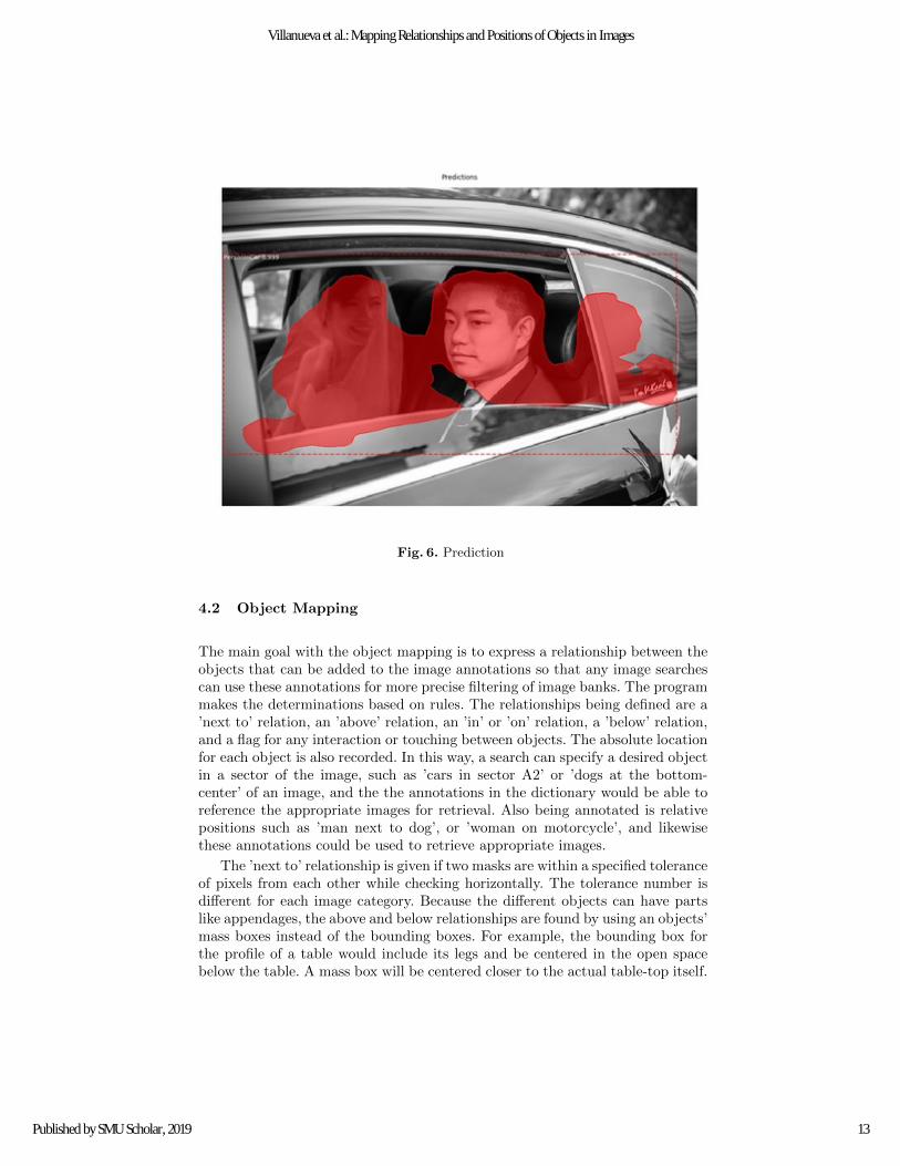
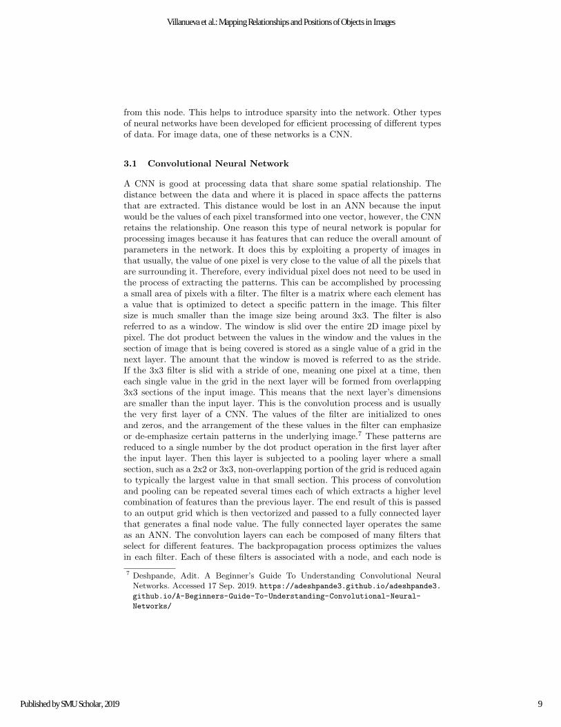
Fig. 6. Prediction

4.2 Object Mapping

The main goal with the object mapping is to express a relationship between theobjects that can be added to the image annotations so that any image searchescan use these annotations for more precise filtering of image banks. The programmakes the determinations based on rules. The relationships being defined are a’next to’ relation, an ’above’ relation, an ’in’ or ’on’ relation, a ’below’ relation,and a flag for any interaction or touching between objects. The absolute locationfor each object is also recorded. In this way, a search can specify a desired objectin a sector of the image, such as ’cars in sector A2’ or ’dogs at the bottom-center’ of an image, and the the annotations in the dictionary would be able toreference the appropriate images for retrieval. Also being annotated is relativepositions such as ’man next to dog’, or ’woman on motorcycle’, and likewisethese annotations could be used to retrieve appropriate images.

The ’next to’ relationship is given if two masks are within a specified toleranceof pixels from each other while checking horizontally. The tolerance number isdifferent for each image category. Because the different objects can have partslike appendages, the above and below relationships are found by using an objects’mass boxes instead of the bounding boxes. For example, the bounding box forthe profile of a table would include its legs and be centered in the open spacebelow the table. A mass box will be centered closer to the actual table-top itself.

13



The mass box for an object is determined by starting with the given coordi-nates of the bounding box and scanning towards the image one axis at a time,one pixel at a time. At each iteration of pixel movement, the total pixels of themask remaining in the box is multiplied by the percentage of pixels of the maskremaining in the box. The coordinate will continue iterating all the way to theother end of the box remembering at what value the product was maximal. Allfour axes are moved in towards the center of the object in this manner.

The ’above’ and ’below’ tags use the center of the mass box of the object whilechecking to what degree the pixels from each object aligned with each other.The ’on’ and ’in’ tags proved troublesome relying on the interaction between anobject’s pixels and another object’s topline to be determined. One other usefulrelationship that is recorded is an interaction between objects where objects areactually touching. First, each mask is artificially inflated by a specified numberof pixels. This is performed by scanning in from all four edges of the image oneaxis at a time. The scanning looks at the specified number of pixels, and if thefirst pixel is False, it performs a logical ’OR’ operation and replaces all pixelsbeing evaluated by the result. After this is completed for each object’s mask, alogical ’AND’ is performed between each mask followed by a search for any Truevalues. If any are found, then the objects are determined to be touching.

5 Analysis and Results

A summary of the performance of the three models primarily used can be seenin Table 1. The testing of the COCO weights with our images was expected tobe a little higher, but even at 82% accuracy, these weights were very serviceable.The model was tested against the same images that were used to generate therelationship tags.

Table 1. Testing of Model Performance.

Model Weights Accuracy

CNN VGG16 94%

CNN VGG16 (Transfer Learning) 72%

Mask R-CNN COCO Mask R-CNN 82%

One interesting thing to note is that the images used for testing the MS-COCO weights as well as the annotation process overwhelmingly had people asthe detected object. This spread can be seen in Figure 7. Though, it makes sensethat people would normally be a part of images in general, it is noteworthy thatmany practice runs were run on controlled sets such as dogs, cats, bikes, carsetc., and the objects being detected does affect the accuracy numbers. Certainmodels just seem to do better with certain objects. The Mask R-CNN modelseems to do very well with people being able to detect a person accurately ifeven the smallest part of any part of the person was in the image.

14



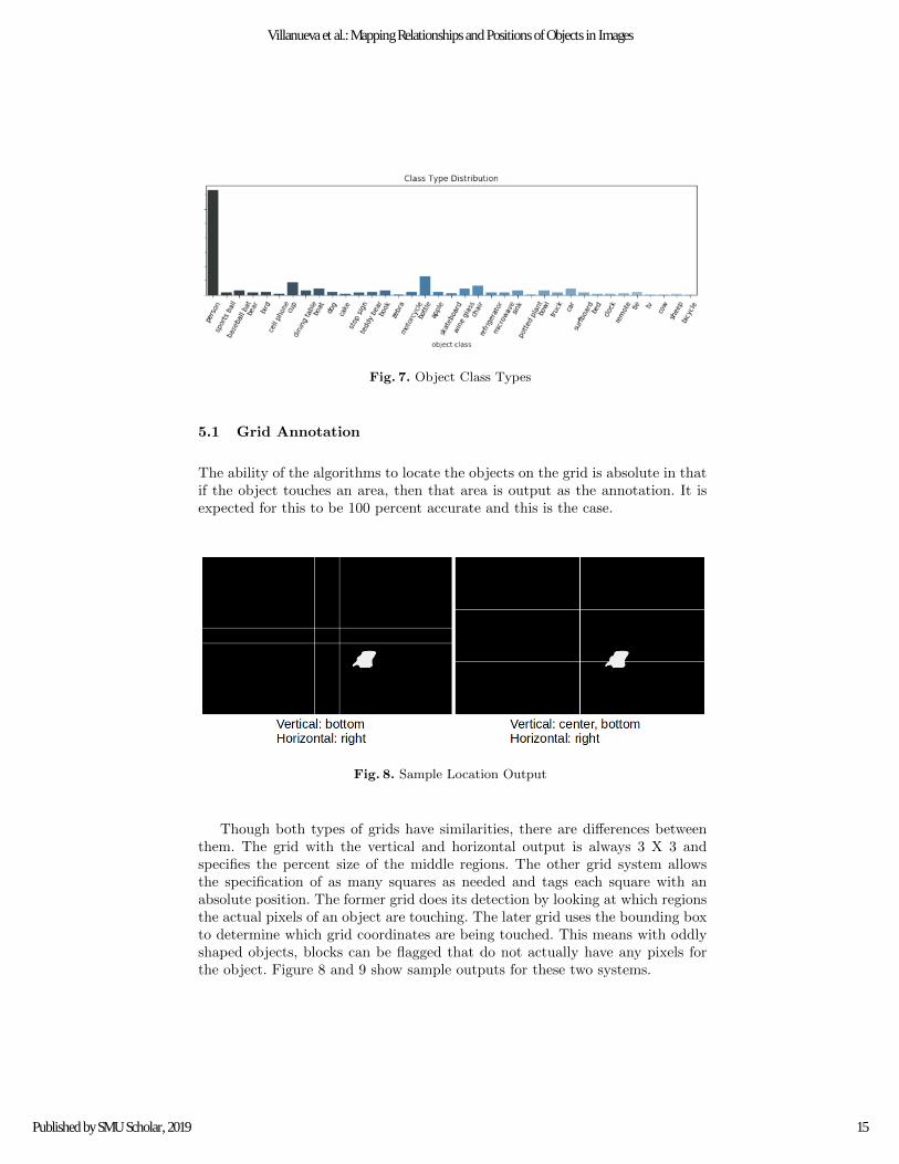
Fig. 7. Object Class Types

5.1 Grid Annotation

The ability of the algorithms to locate the objects on the grid is absolute in thatif the object touches an area, then that area is output as the annotation. It isexpected for this to be 100 percent accurate and this is the case.

Fig. 8. Sample Location Output

Though both types of grids have similarities, there are differences betweenthem. The grid with the vertical and horizontal output is always 3 X 3 andspecifies the percent size of the middle regions. The other grid system allowsthe specification of as many squares as needed and tags each square with anabsolute position. The former grid does its detection by looking at which regionsthe actual pixels of an object are touching. The later grid uses the bounding boxto determine which grid coordinates are being touched. This means with oddlyshaped objects, blocks can be flagged that do not actually have any pixels forthe object. Figure 8 and 9 show sample outputs for these two systems.

15



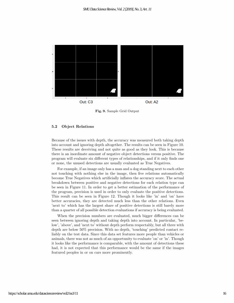
Fig. 9. Sample Grid Output

5.2 Object Relations

Because of the issues with depth, the accuracy was measured both taking depthinto account and ignoring depth altogether. The results can be seen in Figure 10.These results are deceiving and not quite as good as they look. This is becausethere is an inordinate amount of negative object detections versus positive. Theprogram will evaluate six different types of relationships, and if it only finds oneor none, the unused detections are usually evaluated as True Negatives.

For example, if an image only has a man and a dog standing next to each othernot touching with nothing else in the image, then five relations automaticallybecome True Negatives which artificially inflates the accuracy score. The actualbreakdown between positive and negative detections for each relation type canbe seen in Figure 11. In order to get a better estimation of the performance ofthe program, precision is used in order to only evaluate the positive detections.This result can be seen in Figure 12. Though it looks like ’in’ and ’on’ havebetter accuracies, they are detected much less than the other relations. Even’next to’ which has the largest share of positive detections is still barely morethan a quarter of all possible detection evaluations if accuracy is being evaluated.

When the precision numbers are evaluated, much bigger differences can beseen between ignoring depth and taking depth into account. In particular, ’be-low’, ’above’, and ’next to’ without depth perform respectably, but all three withdepth are below 50% precision. With no depth, ’touching’ predicted contact re-liably on the test data. Since this data set features more people than vehicles oranimals, there was not as much of an opportunity to evaluate ’on’ or ’in’. Thoughit looks like the performance is comparable, with the amount of detections thesehad, it is not expected that this performance would be the same if the imagesfeatured peoples in or on cars more prominently.

16



Fig. 10. Relationship Accuracy

Fig. 11. Relationship Positive/Negative Splits

17



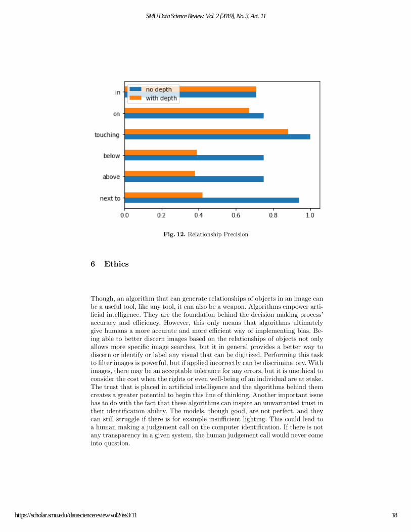
Fig. 12. Relationship Precision

6 Ethics

Though, an algorithm that can generate relationships of objects in an image canbe a useful tool, like any tool, it can also be a weapon. Algorithms empower arti-ficial intelligence. They are the foundation behind the decision making process’accuracy and efficiency. However, this only means that algorithms ultimatelygive humans a more accurate and more efficient way of implementing bias. Be-ing able to better discern images based on the relationships of objects not onlyallows more specific image searches, but it in general provides a better way todiscern or identify or label any visual that can be digitized. Performing this taskto filter images is powerful, but if applied incorrectly can be discriminatory. Withimages, there may be an acceptable tolerance for any errors, but it is unethical toconsider the cost when the rights or even well-being of an individual are at stake.The trust that is placed in artificial intelligence and the algorithms behind themcreates a greater potential to begin this line of thinking. Another important issuehas to do with the fact that these algorithms can inspire an unwarranted trust intheir identification ability. The models, though good, are not perfect, and theycan still struggle if there is for example insufficient lighting. This could lead toa human making a judgement call on the computer identification. If there is notany transparency in a given system, the human judgement call would never comeinto question.

18



7 Conclusions

Much information can be determined from the pixel and bounding box outputsof the Mask R-CNN. They can be used to determine the absolute location ofa detected object in the image. To a lesser degree, they can also be used todetermine the relationship of a detected object to other detected objects. Partof the issue with relative relationship determination using only bounding boxesand masks is the variability created by all the different types of camera angles,plus the variability in the different sizes of objects being detected, as well asthe fact that the detection is good enough to recognize only partial pieces ofan images as a whole. Several pictures had just a hand or foot recognized asa person. Being able to reliably describe a relationship between objects wouldrequire collection of many different types of images of that particular object.This could aid in helping a rule based method like this. However, the absoluterelationships can reliably be associated with keywords which can be used tomore precisely filter large banks of images. The relative relationships tags canbe used as well, but dealing with the issues of depth, makes this model performat best in the 50% precision range. This reduced performance, however, may besufficient enough to help in sorting through large banks of images.

References

1. Bowen, C.e.a.: Revisiting rcnn: On awakening the classification power of fasterrcnn. In: arXiv.org (2018)

2. Burkov, A.: The Hundred-Page Machine Learning Book. Andriy Burkov (2019)

3. Gao, J.e.a.: Note-rcnn: Noise tolerant ensemble rcnn for semi-supervised objectdetection. In: arXiv.org (2018)

4. Johnson, J.: Adapting mask-rcnn for automatic nucleus segmentation. In: arXiv.org(2018)

5. Lei, Q., e.a.: Research on human target recognition algorithm of home servicerobot based on fast-rcnn. 10th International Conference on Intelligent ComputationTechnology and Automation (ICICTA) 2017, 47–55 (2017)

6. Lin, T.Y., Maire, M., Belongie, S., Bourdev, L., Girshick, R., Hays, J., Perona, P.,Ramanan, D., Zitnick, C.L., Dollar, P.: Microsoft coco: Common objects in context(2014)

7. Liu, Y.e.a.: A method for singular points detection based on faster-rcnn. In: AppliedSciences 8.10 (2018) (2018)

8. Malhotra, K.R.e.a.: Autonomous detection of disruptions in the intensive care unitusing deep mask rcnn. IEEE Computer Society Conference on Computer Visionand Pattern Recognition Workshops 2018, 1944–1946 (2018)

9. Sommer, L.e.a.: A-fast-rcnn: Hard positive generation via adversary for objectdetection. In: 018 25th IEEE International Conference on Image Processing (ICIP).p. 3054–3058 (2018)

10. Sorokin, A.: Lesion analysis and diagnosis with mask-rcnn. In: arXiv.org (2018)

11. Sun, Xudong, W.P., Hoi, S.C.: Face detection using deep learning: An improvedfaster rcnn approach. In: Neurocomputing 299.C (2018). p. 42–50 (2018)

19



12. Ullah, A.e.a.: Pedestrian detection in infrared images using fast rcnn. In: 2018Eighth International Conference on Image Processing Theory, Tools and Applica-tions (IPTA). pp. 1–6 (2018)

13. Wang, Xiaolong, S.A., Gupta, A.: A-fast-rcnn: Hard positive generation via adver-sary for object detection. In: arXiv.org (2017)

14. Yu, Y.e.a.: Fruit detection for strawberry harvesting robot in non-structural en-vironment based on mask-rcnn. Computers and Electronics in Agriculture 163(2019)

15. Zhang, W.: Characters detection on namecard with faster rcnn. In: arXiv.org(2018)

16. Zhang, Changzheng, X.X., Tu, D.: Face detection using improved faster rcnn. In:arXiv.org (2018)

20



mapping relationships and positions of objects in images

Documents