mapping secondary succession species in agricultural

Mapping secondary successionspecies in agricultural landscape withthe use of hyperspectral andairborne laser scanning data

Aleksandra RadeckaDorota Michalska-HejdukKatarzyna Osińska-SkotakAdam KaniaKonrad GórskiWojciech Ostrowski

Aleksandra Radecka, Dorota Michalska-Hejduk, Katarzyna Osińska-Skotak, Adam Kania, Konrad Górski,Wojciech Ostrowski, “Mapping secondary succession species in agricultural landscape with the use ofhyperspectral and airborne laser scanning data,” J. Appl. Remote Sens. 13(3), 034502 (2019),doi: 10.1117/1.JRS.13.034502.

Downloaded From: https://www.spiedigitallibrary.org/journals/Journal-of-Applied-Remote-Sensing on 21 Nov 2021Terms of Use: https://www.spiedigitallibrary.org/terms-of-use

Mapping secondary succession species in agriculturallandscape with the use of hyperspectral and airborne

laser scanning data

Aleksandra Radecka,a,* Dorota Michalska-Hejduk,b

Katarzyna Osińska-Skotak,a Adam Kania,c Konrad Górski,a

and Wojciech OstrowskiaaWarsaw University of Technology, Department of Photogrammetry, Remote Sensing and

Spatial Information Systems, Faculty of Geodesy and Cartography, Warsaw, PolandbUniversity of Lodz, Department of Geobotany and Plant Ecology, Lodz, Poland

cDefinity Ltd., Sw. Judy Tadeusza, Wroclaw, Poland

Abstract. Secondary succession is a process that is often observed taking place in former agri-cultural ecosystems. Its characteristics are especially important in protected areas, for the pur-poses of monitoring and protective measures. Effective mapping of succession is facilitated bythe development of automated methodologies based on remote sensing data, which are capableof complementing traditional field research. The objective of this work is to determine whetherthe classification of high-resolution hyperspectral and light detection and ranging (LiDAR) datawith the use of the random forest algorithm enables us to produce an accurate succession speciesmap. First, feature extraction techniques are applied to 1-m hyperspectral images and a∼7 point∕m2 dense point cloud. Minimum noise fraction layers and vegetation indices are cal-culated from the hyperspectral data and geometry related indices from the LiDAR data. Finally,the recursive feature elimination algorithm is applied to the combined dataset and the referencepolygons to select the optimal set of features for subsequent classification. The results indicatethat the proposed methodology has the potential to be used operationally. The final classificationproduct is characterized by a relatively high Cohen’s kappa value of 0.68, with single speciesclassified with various accuracies, expressed by F1 scores ranging from 0.45 to 0.87. © TheAuthors. Published by SPIE under a Creative Commons Attribution 4.0 Unported License.Distribution or reproduction of this work in whole or in part requires full attribution of the original pub-lication, including its DOI. [DOI: 10.1117/1.JRS.13.034502]

Keywords: ecological process; Natura 2000 monitoring; hyperspectral imaging; light detectionand ranging data; data fusion; random forest.

Paper 190042 received Jan. 18, 2019; accepted for publication Jun. 20, 2019; published onlineJul. 16, 2019.

1 Introduction

The succession process is currently the subject of a large number of research projects all overthe world, for example in Europe,1–3 North America,4–9 South America,10–12 and also in Asia.13

The reason behind the interest in this topic is undoubtedly connected with its significance, whichcan be seen from three different perspectives. In some areas, similar to the current research, thesecondary succession is perceived as a threat to certain ecosystems. This is because large areas ofseminatural nonforest communities, e.g., grasslands and meadows (and especially the less pro-ductive parts) have been abandoned, resulting in secondary succession.14–16 The cessation ofmowing or grazing allows species with clonal growth to complete their full development andinduces changes in the quantitative and spatial structures of plant communities.17 One of theresults of this process is the disappearance of some groups of species (e.g., heliophilous ones)and the formation of shrub and forest communities created by species that are better adapted topoor light conditions. This situation leads to changes in the composition of species in an eco-system,18,19 in not only plant species but also animal communities.20–22 As a result, secondary

*Address all correspondence to Aleksandra Radecka, E-mail: [email protected]

Journal of Applied Remote Sensing 034502-1 Jul–Sep 2019 • Vol. 13(3)


https://doi.org/10.1117/1.JRS.13.034502

https://doi.org/10.1117/1.JRS.13.034502

https://doi.org/10.1117/1.JRS.13.034502

https://doi.org/10.1117/1.JRS.13.034502

https://doi.org/10.1117/1.JRS.13.034502

mailto:[email protected]




succession also leads to changes at the landscape level. This standpoint is generally taken if theprocess threatens the existence of protected habitats or the vegetation involves invasive species.This view is represented by Szostak et al.,2 Szostak et al.,3 Vanderlinder et al.,7 and others. Inother places, secondary succession is recognized as having a highly positive impact on climateand biodiversity and as an important reservoir of carbon.8,9,11 In most cases, however, the impor-tance of secondary succession is simply explained by the large size of the terrain encompassed,land use and land cover changes, and the resultant need to assess its influence on ecosystemfunctions and services.1,4–6,10,12,13

Regardless of the reason, studies of secondary succession focus mainly on identifying theplaces, in which the succession occurs, estimating the size of this area3,7 and describing thestages of the process,1,4–6,9–13 and rarely on determining other characteristics such as the standage or species richness.8 To the authors’ knowledge, few research projects have investigated thesubject of the differentiation of succession species. Although many studies have focused on theidentification of tree, shrub, or other plant species, only a small number of these have involvedthe mapping of succession tree species.23,24 The majority of studies have been carried out in anurban environment25–27 or in different types of mature forests.28–30 This indicates a need forfurther research into succession-specific challenges, e.g., the possibilities of distinguishing dif-ferent succession species based on their spectral and geometrical characteristics or approaches tothe processing of reference data. This study is a response to these needs. Its primary goals are to(i) examine the possibility of effectively mapping succession species present in an agriculturallandscape via the use of simultaneously acquired high-resolution hyperspectral and light detec-tion and ranging (LiDAR) data and (ii) to investigate the most important features of tree-speciesclassification using the recursive feature elimination (RFE) algorithm.

2 Study Area

The study area is located in the southern part of Poland, in the Silesian Voivodeship, nearCzestochowa city (50°45” N; 19°17” E). It encompasses an area of about 25 km2. This area,according to the physiographic regionalization of Poland,31 is located in the macroregion of theKrakow-Czestochowa Upland, the mesoregion of the Czestochowa Upland, and the microregionof the Mirowsko-Olsztynska Upland. The area is located in the Warta basin, east ofCzestochowa, at the northern end of the Czestochowa Upland, being an enclave of natural andseminatural ecosystems, present between the highly urbanized areas of Silesia and Czestochowaindustrial districts.

The thermal conditions of the area are typical for the climatic region of the central highlands,with an average annual temperature of 7.6°C. The coldest months of the year are January andFebruary, and the average temperatures during these months are relatively low, approaching−3°C. The average annual air temperature amplitude is typical of western and centralPoland, amounting to 20.8°C. Due to the thermal conditions, the vegetation period lasts for about210 days per year. Snow cover, for which the durability depends on a negative air temperature,persists in the upland area for about 50 to 70 days. Precipitation is relatively high, exceeding700 mm per year.

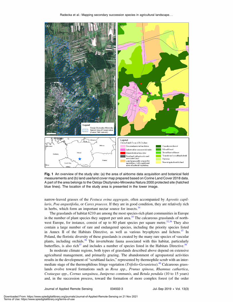
The area includes a complex of limestone hills (absolute heights range between 278 and374 m) with numerous karst forms, such as caves, crosses, fissures, sinkholes, and so on.The hills are covered by natural forest communities (mostly beech and hornbeam forests) orseminatural species-rich grasslands.32 The areas adjacent to the hills are occupied by cultivatedfields and pine forests. The area is characterized by a wide diversity of habitats, with a consid-erable wealth of plant and animal species;33 it is, therefore, protected as a Natura 2000 site knownas Ostoja Olsztynsko-Mirowska (PLH240015) (Fig. 1).

The most important threatened nonforest habitats in this area are two types of grassland(codes 6120 and 6210), which were analyzed in this research. The first type, habitat 6120, con-sists of dry, frequently open grasslands on more or less calcareous sands with a subcontinentalcentre of distribution, comprising seminatural, moderately open to closed, relatively low-grownmesoxeric grasslands on slightly calcareous sands in the lowlands, and medium height moun-tains throughout temperate Europe. These grasslands are mostly dominated by tussock-forming,

Radecka et al.: Mapping secondary succession species in agricultural landscape. . .



narrow-leaved grasses of the Festuca ovina aggregate, often accompanied by Agrostis capil-laris, Poa angustifolia, or Carex praecox. If they are in good condition, they are relatively richin herbs, which form an important nectar source for insects.34

The grasslands of habitat 6210 are among the most species-rich plant communities in Europein the number of plant species they support per unit area.35 The calcareous grasslands of north-west Europe, for instance, consist of up to 80 plant species per square metre.32,36 They alsocontain a large number of rare and endangered species, including the priority species listedin Annex II of the Habitats Directive, as well as various bryophytes and lichens.37 InPoland, the floristic diversity of these grasslands is created by the many rare species of vascularplants, including orchids.38 The invertebrate fauna associated with this habitat, particularlybutterflies, is also rich37 and includes a number of species listed in the Habitats Directive.39

In moderate climate regions, both types of grasslands described above depend on extensiveagricultural management, and primarily grazing. The abandonment of agropastoral activitiesresults in the development of “scrubland facies,” represented by thermophile scrub with an inter-mediate stage of the thermophilous fringe vegetation (Trifolio-Geranietea).40 Calcareous grass-lands evolve toward formations such as Rosa spp., Prunus spinosa, Rhamnus cathartica,Crataegus spp., Cornus sanguinea, Juniperus communis, and Betula pendula (10 to 15 years)and, in the succession process, toward the formation of more complex forest (of the order

Fig. 1 An overview of the study site: (a) the area of airborne data acquisition and botanical fieldmeasurements and (b) land use/land cover map prepared based on Corine Land Cover 2018 data.A part of the area belongs to the Ostoja Olsztynsko-Mirowska Natura 2000 protected site (hatchedblue lines). The location of the study area is presented in the lower image.




Fagetalia), over 70 years or more.41 Scrub encroachment is the most frequently documentedreason for change in 6210* sites; this is considered to be an acute threat because it can resultin an increase in soil nutrients and a decline in the richness of grassland species42 as the suc-cession progresses.

An overview of the landscape and selected succession species of the study area is presentedin Fig. 2.

3 Materials and Methods

3.1 Data

The research described here was carried out using two types of data: remote sensing and fielddata. Remotely acquired data consisted of hyperspectral images, RGB images, and LiDAR data(Fig. 3). The technical parameters characterizing the sensors and the data they provided are pre-sented in Table 1. The collected field data could be divided into two groups: the first was spec-trometer measurements that were needed for the evaluation of the atmospheric correction ofhyperspectral imagery, and the second comprised botanical measurements acquired in the formof GPS points, with supplementary attributes characterizing the trees and shrubs occurring in thearea under study (i.e., the height of an object, its crown density, crown radius, level of discolor-ation, level of defoliation, and neighboring vegetation type). The species were divided into twogroups: (i) species playing a role in the early stages of the succession process, referred to as“promoters” (seven species) and (ii) nonsuccessive species referred to here as “other,” whichcomprised the remainder of a diverse range of species occurring in the study area. The totalnumber of collected polygons was 406 (Fig. 4); after processing, they served as a classificationreference.

It is especially important that all of the data mentioned already were acquired simultaneously.Acquiring all remote sensing data at the same time enabled subsequent uncomplicated and

Fig. 2 Succession promoters present in the Ostoja Olsztynsko-Mirowska Natura 2000 protectedsite: (a) grasslands being overgrown by Scots pine, Pinus sylvestris, silver birch, Betula pendula,and common hazel, Corylus avellana; (b) common juniper, Juniperus communis, and buckthorn,Rhamnus cathartica, on a limestone hill; (c) silver birch, Betula pendula; (d) hawthorn, Crataegusspp.; (e) Scots pine, Pinus sylvestris.




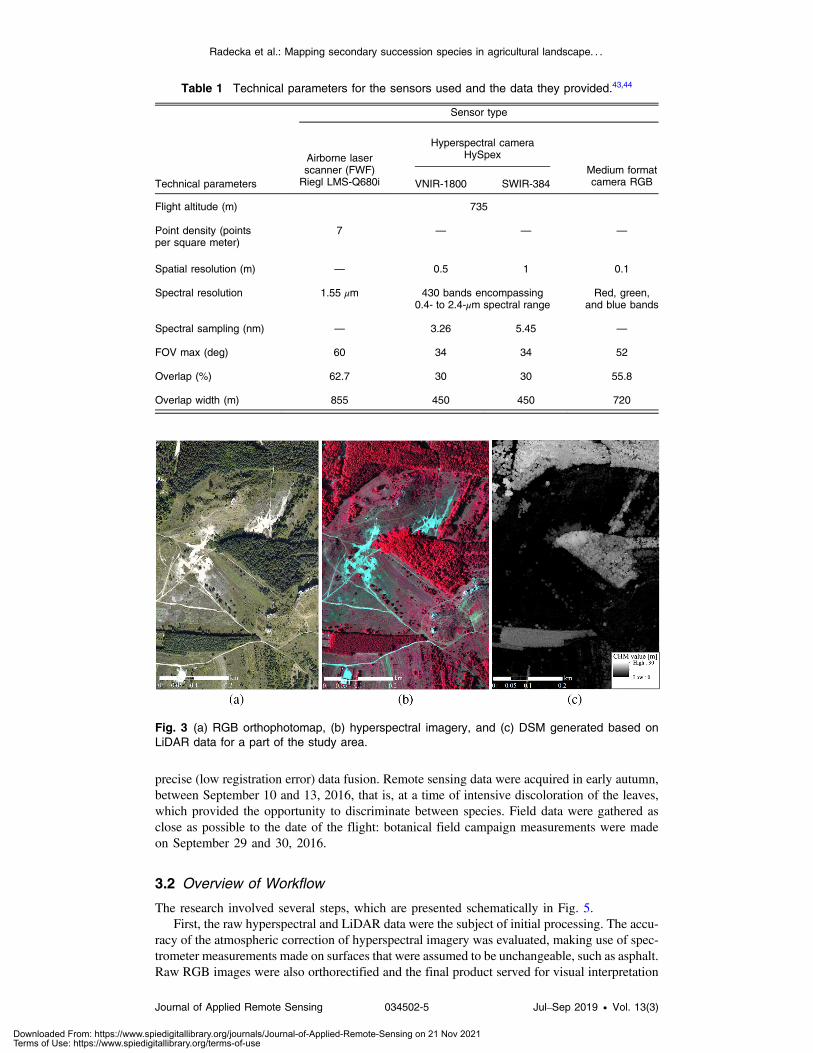
precise (low registration error) data fusion. Remote sensing data were acquired in early autumn,between September 10 and 13, 2016, that is, at a time of intensive discoloration of the leaves,which provided the opportunity to discriminate between species. Field data were gathered asclose as possible to the date of the flight: botanical field campaign measurements were madeon September 29 and 30, 2016.

3.2 Overview of Workflow

The research involved several steps, which are presented schematically in Fig. 5.First, the raw hyperspectral and LiDAR data were the subject of initial processing. The accu-

racy of the atmospheric correction of hyperspectral imagery was evaluated, making use of spec-trometer measurements made on surfaces that were assumed to be unchangeable, such as asphalt.Raw RGB images were also orthorectified and the final product served for visual interpretation

Fig. 3 (a) RGB orthophotomap, (b) hyperspectral imagery, and (c) DSM generated based onLiDAR data for a part of the study area.

Table 1 Technical parameters for the sensors used and the data they provided.43,44

Technical parameters

Sensor type

Airborne laserscanner (FWF)Riegl LMS-Q680i

Hyperspectral cameraHySpex

Medium formatcamera RGBVNIR-1800 SWIR-384

Flight altitude (m) 735

Point density (pointsper square meter)

7 — — —

Spatial resolution (m) — 0.5 1 0.1

Spectral resolution 1.55 μm 430 bands encompassing0.4- to 2.4-μm spectral range

Red, green,and blue bands

Spectral sampling (nm) — 3.26 5.45 —

FOV max (deg) 60 34 34 52

Overlap (%) 62.7 30 30 55.8

Overlap width (m) 855 450 450 720




Fig. 5 The main steps of the research described in this paper.

Fig. 4 Location of measured trees and shrubs as referenced data.




throughout all the stages of the research. In the second step, dedicated to feature extraction,preprocessed hyperspectral and LiDAR data were used to prepare new informative products.The hyperspectral imagery alone and the datasets created by combining it with the LiDAR dataare known to be powerful sources of information about vegetation and have been used in manyresearch studies involving species discrimination.23,25,26,28–30,45

In the next stage, botanical field measurements were manually processed, which made itpossible to determine the outlines of the research objects. The polygons created at this stagewere later used as a reference for species classification. The supervised feature selection donein the fourth step made it possible to choose an optimal set of features for subsequent classi-fication. The result of the classification process was then masked based on three criteria: height,land cover, and the presence of shadows. In the final step, the result was evaluated using stat-istical measures.

The whole process is described in detail in the following sections, which discuss each of theaforementioned issues.

3.2.1 Preparation of reference data

The source data for preparation of the reference polygons were botanical field measurementsindicating the location and characteristics of the research objects, which were trees and shrubs.Points were collected using a differential global positioning system (DGPS) receiver, with errorvalues of between 0.3 and 0.5 m on average and never exceeding 1 m. Although the measure-ment accuracy was high, the creation of a reference polygon in the form of a buffer around apoint would not be an ideal approach. Bearing in mind the relationship between the measurementaccuracy and the size of the object, it could be expected that several valid pixels would be omit-ted and some invalid ones added to a reference set in this way.

The procedure chosen in the first step assumed the creation of a buffer whose radius wasdetermined to be the object’s radius, as measured by the botany expert in the field, plus a few (2to 3) meters. The additional enlargement of the buffer was done to account for a DGPS meas-urement accuracy, as well as possible little misalignments between the measurements and remotesensing data. The prepared vectors, i.e., circles, were then projected onto the pixel grid of thehyperspectral data, dividing each circle into a number of elements reflecting pixels. In the laststep, these elements were visually evaluated against the presence of an object (a tree or a shrub),mixed pixels on the border of an object and its surroundings, and the presence of shadows. Thiswork was carried out by a botany expert, who utilized many different materials: orthophotos,hyperspectral mosaic, and a crown height model (CHM). An example of the resultant polygonscan be seen in Fig. 6.

A few nonsuccessive species present on the research area occurred mostly in high foreststands, and therefore, reference polygons created for these specimens could not be based onprecise dGPS measurements. However, they were highly different spectrally and in crown shape,thus easy to identify visually and vectorize on the remote sensing materials.

Finally, the prepared reference polygons were divided into training and validation samplesusing stratified random sampling. Each stratum was a combination of a species and the values ofparameters that in the authors’ opinion characterized the most important of its features: its height,crown density, and size defined by the radius. This operation ensured diversification of both thetraining and the validation sets for each species. The final number of reference polygons used inthe classification process is presented in Table 2.

3.2.2 LiDAR data processing

Raw LiDAR data were preprocessed and oriented according to the standard procedure in Riegl’sdedicated software RiProcess (RIEGL Laser Measurement Systems GmbH, Horn, Austria).46

Full-wave signal decomposition was also performed in Riegl’s software (RIEGL LaserMeasurement Systems GmbH, Horn, Austria),47 using a Gaussian decomposition techniqueto describe the recorded signal, its extracted echoes and their descriptive parameters such asthe echo width and amplitude. Next, the preprocessed point clouds were classified usingAxelsson’s algorithm48 into ground, vegetation, and unclassified, according to the ASPRS




LAS classification standard, in Terrasolid software (Terrasolid Ltd., Helsinki, Finland).49 Theresult of the automatic classification was manually checked using cross sections views of thepoint cloud in TerraScan and all detected errors were manually corrected by the airborne dataprovider.

In the next step, LiDAR-based rasters, an input dataset for species classification, were gen-erated. The processing of point clouds was performed using TU Wien OPALS software50 andstandard rasterization methods. To calculate several raster models, several additional calculationswere needed directly in the point clouds, for example for the normalized height or echo ratioparameter51 of each point. The final raster datasets were divided into three groups based on thepoint cloud class used to create each raster and according to the scheme used in BCAL soft-ware:52 an ALL group (generated based on the points of all classes except noise), a GRD group(generated based on ground points only), and a VEG group (generated based on vegetation

Table 2 The number of reference polygons used in the classification process.

Species name Number of calibration polygons Number of validation polygons

Silver birch, Betula pendula 14 18

Scots pine, Pinus sylvestris 15 19

Common juniper, Juniperus communis 20 25

Buckthorn, Rhamnus cathartica 13 20

Hawthorn, Crataegus spp. 15 19

Blackthorn, Prunus spinosa 13 17

Common pear, Pyrus communis 13 20

Other species 71 94

Fig. 6 (a) CHM, (b) hyperspectral imagery, and (c)–(f) overlaid with the reference polygons andclose-up of the study area fragment.




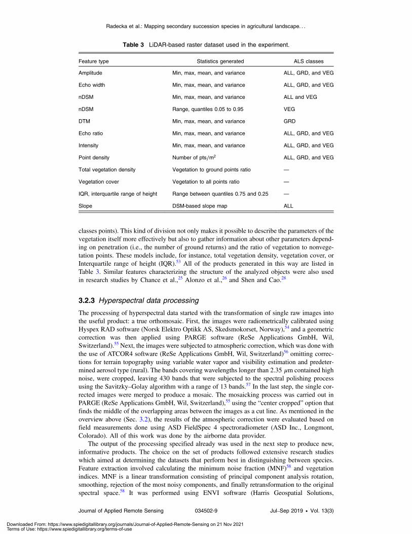
classes points). This kind of division not only makes it possible to describe the parameters of thevegetation itself more effectively but also to gather information about other parameters depend-ing on penetration (i.e., the number of ground returns) and the ratio of vegetation to nonvege-tation points. These models include, for instance, total vegetation density, vegetation cover, orInterquartile range of height (IQR).53 All of the products generated in this way are listed inTable 3. Similar features characterizing the structure of the analyzed objects were also usedin research studies by Chance et al.,25 Alonzo et al.,26 and Shen and Cao.28

3.2.3 Hyperspectral data processing

The processing of hyperspectral data started with the transformation of single raw images intothe useful product: a true orthomosaic. First, the images were radiometrically calibrated usingHyspex RAD software (Norsk Elektro Optikk AS, Skedsmokorset, Norway),54 and a geometriccorrection was then applied using PARGE software (ReSe Applications GmbH, Wil,Switzerland).55 Next, the images were subjected to atmospheric correction, which was done withthe use of ATCOR4 software (ReSe Applications GmbH, Wil, Switzerland)56 omitting correc-tions for terrain topography using variable water vapor and visibility estimation and predeter-mined aerosol type (rural). The bands covering wavelengths longer than 2.35 μm contained highnoise, were cropped, leaving 430 bands that were subjected to the spectral polishing processusing the Savitzky–Golay algorithm with a range of 13 bands.57 In the last step, the single cor-rected images were merged to produce a mosaic. The mosaicking process was carried out inPARGE (ReSe Applications GmbH, Wil, Switzerland),55 using the “center cropped” option thatfinds the middle of the overlapping areas between the images as a cut line. As mentioned in theoverview above (Sec. 3.2), the results of the atmospheric correction were evaluated based onfield measurements done using ASD FieldSpec 4 spectroradiometer (ASD Inc., Longmont,Colorado). All of this work was done by the airborne data provider.

The output of the processing specified already was used in the next step to produce new,informative products. The choice on the set of products followed extensive research studieswhich aimed at determining the datasets that perform best in distinguishing between species.Feature extraction involved calculating the minimum noise fraction (MNF)58 and vegetationindices. MNF is a linear transformation consisting of principal component analysis rotation,smoothing, rejection of the most noisy components, and finally retransformation to the originalspectral space.58 It was performed using ENVI software (Harris Geospatial Solutions,

Table 3 LiDAR-based raster dataset used in the experiment.

Feature type Statistics generated ALS classes

Amplitude Min, max, mean, and variance ALL, GRD, and VEG

Echo width Min, max, mean, and variance ALL, GRD, and VEG

nDSM Min, max, mean, and variance ALL and VEG

nDSM Range, quantiles 0.05 to 0.95 VEG

DTM Min, max, mean, and variance GRD

Echo ratio Min, max, mean, and variance ALL, GRD, and VEG

Intensity Min, max, mean, and variance ALL, GRD, and VEG

Point density Number of pts∕m2 ALL, GRD, and VEG

Total vegetation density Vegetation to ground points ratio —

Vegetation cover Vegetation to all points ratio —

IQR, interquartile range of height Range between quantiles 0.75 and 0.25 —

Slope DSM-based slope map ALL




Broomfield, Colorado)59 and the resultant layers were put through a preselection process, inwhich the noisy layers were deleted and only informative layers were kept. Vegetation indiceswere calculated using both ENVI (Harris Geospatial Solutions, Broomfield, Colorado)59 andEnMAP-Box software (The Environmental Mapping and Analysis Program, EarthObservation Center EOC of DLR, Germany),60 and many different vegetation features werecharacterized.

3.2.4 Feature selection

In the next step, the products of the LiDAR and hyperspectral data processing underwent a fea-ture selection procedure. As described by Archibald and Fann61 and Singh et al.,62 the appli-cation of feature selection is an important step that should be implemented before classification,as it can reduce the time taken to build the learning model and increase the accuracy of theclassification result, improving its generalization ability as well. These benefits can be achievedby removing redundant and insignificant features. In this research, the feature selection processwas performed using the RFE algorithm based on a random forest estimate of feature impor-tance. The chosen algorithm is categorized in the literature as a wrapper approach.62

As a standard part of the random forest learning algorithm, an internal assessment of thevariable importance is calculated. For every model learned using the random forest classifier,an estimation of the importance of each feature used for classification is available in the form of avalue between 0.0 and 1.0.

When used in an RFE workflow, this possibility is used in the following way. First, a clas-sifier is learned using the full set of features. The resulting importance of the variable (or feature)is then analyzed and typically one feature (or sometimes more) with the lowest score (i.e.,the least useful in discriminating between target classes) is eliminated from the feature set.The next round of learning is then performed, eliminating the next weakest feature, and thisprocedure is repeated until all the features are exhausted or the accuracy of the model startsdropping significantly, which happens as the number of features gets too small to discriminatethe classes.

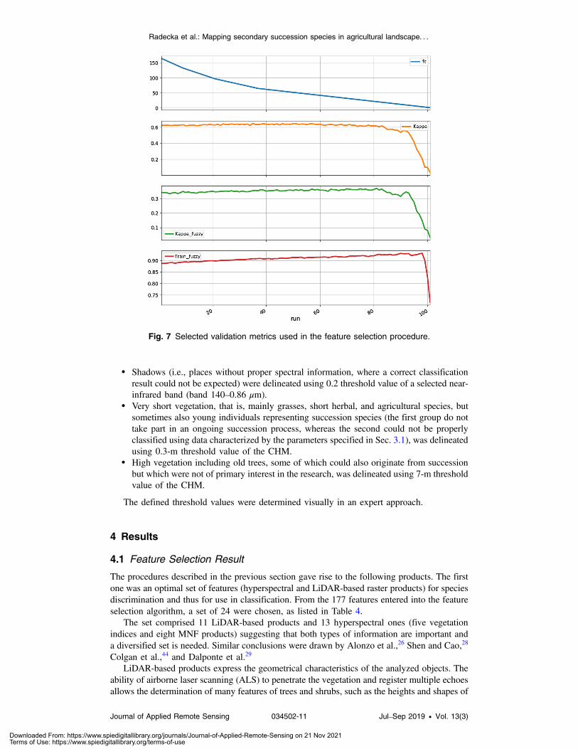
A full set of validation metrics was calculated at each stage of this procedure (i.e., number offeatures, Kappa values calculated in both hard and fuzzy way, validation accuracies on the train-ing, as well as on validation set), then the metrics from the whole procedure were plotted on agraph. Example of the selected metrics is presented in Fig. 7. The number of features considered“best” was selected after manual analysis, aiming for relatively small number of most inform-ative features still resulting in good learning/validation performance for a given dataset.

These properties of the algorithm made it possible to choose an optimal set of features forclassification, a combination of hyperspectral and LiDAR-based layers, making use of Cohen’skappa value63 to characterize each of the models.

3.2.5 Classification and postprocessing

As indicated in the previous sections, the classification involved making use of both the set oflayers determined during the feature selection stage and the reference polygons. The classifi-cation was done using a pixel-based random forest algorithm, treating the succession speciesas separate classes, and the rest of the species present in the research area as one class, in asimilar way to Colgan et al.45 and Graves et al.23

The result obtained from a classifier was an image indicating one chosen class for each pixel,meaning that the research area was completely classified. Given the way in which the algorithmworks, there was no measure that specified the degree of similarity between the model (trainingdata) and each pixel analyzed. Therefore, areas that were outside the interest of the researchcould not be eliminated automatically in the same step.

The exclusion process was realized by preparing a specific mask. Four types of deletioncriteria were defined:

• Anthropogenic objects (i.e., nonvegetative areas outside the analysis in the research) wereselected using 0.4 threshold value of the normalized difference vegetation index (NDVI).




• Shadows (i.e., places without proper spectral information, where a correct classificationresult could not be expected) were delineated using 0.2 threshold value of a selected near-infrared band (band 140–0.86 μm).

• Very short vegetation, that is, mainly grasses, short herbal, and agricultural species, butsometimes also young individuals representing succession species (the first group do nottake part in an ongoing succession process, whereas the second could not be properlyclassified using data characterized by the parameters specified in Sec. 3.1), was delineatedusing 0.3-m threshold value of the CHM.

• High vegetation including old trees, some of which could also originate from successionbut which were not of primary interest in the research, was delineated using 7-m thresholdvalue of the CHM.

The defined threshold values were determined visually in an expert approach.

4 Results

4.1 Feature Selection Result

The procedures described in the previous section gave rise to the following products. The firstone was an optimal set of features (hyperspectral and LiDAR-based raster products) for speciesdiscrimination and thus for use in classification. From the 177 features entered into the featureselection algorithm, a set of 24 were chosen, as listed in Table 4.

The set comprised 11 LiDAR-based products and 13 hyperspectral ones (five vegetationindices and eight MNF products) suggesting that both types of information are important anda diversified set is needed. Similar conclusions were drawn by Alonzo et al.,26 Shen and Cao,28

Colgan et al.,44 and Dalponte et al.29

LiDAR-based products express the geometrical characteristics of the analyzed objects. Theability of airborne laser scanning (ALS) to penetrate the vegetation and register multiple echoesallows the determination of many features of trees and shrubs, such as the heights and shapes of

Fig. 7 Selected validation metrics used in the feature selection procedure.




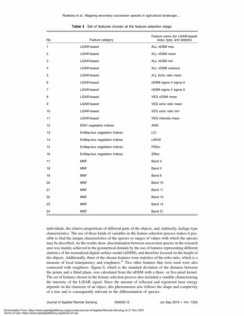
individuals, the relative proportions of different parts of the objects, and, indirectly, leafage-typecharacteristics. The use of these kinds of variables in the feature selection process makes it pos-sible to find the unique characteristics of the species or ranges of values with which the speciesmay be described. As the results show, discrimination between succession species in the researcharea was mainly achieved in the geometrical domain by the use of features representing differentstatistics of the normalized digital surface model (nDSM), and therefore focused on the height ofthe objects. Additionally, three of the chosen features were statistics of the echo ratio, which is ameasure of local transparency and roughness.51 Two other features that were used were alsoconnected with roughness. Sigma 0, which is the standard deviation of the distance betweenthe points and a fitted plane, was calculated from the nDSM with a three- or five-pixel kernel.The set of features chosen in the feature selection process also included a variable characterizingthe intensity of the LiDAR signal. Since the amount of reflected and registered laser energydepends on the character of an object, this phenomenon also follows the shape and complexityof a tree and is consequently relevant in the differentiation of species.

Table 4 Set of features chosen at the feature selection stage.

No. Feature categoryFeature name (for LiDAR-based:

class, type, and statistic)

1 LiDAR-based ALL nDSM max

2 LiDAR-based ALL nDSM mean

3 LiDAR-based ALL nDSM min

4 LiDAR-based ALL nDSM variance

5 LiDAR-based ALL Echo ratio mean

6 LiDAR-based nDSM sigma 3 sigma 0

7 LiDAR-based nDSM sigma 5 sigma 0

8 LiDAR-based VEG nDSM mean

9 LiDAR-based VEG echo ratio mean

10 LiDAR-based VEG echo ratio min

11 LiDAR-based VEG intensity mean

12 ENVI vegetation indices ARI2

13 EnMap-box vegetation indices LCI

14 EnMap-box vegetation indices LWVI2

15 EnMap-box vegetation indices PSSrc

16 EnMap-box vegetation indices SRtot

17 MNF Band 3

18 MNF Band 5

19 MNF Band 6

20 MNF Band 10

21 MNF Band 11

22 MNF Band 13

23 MNF Band 14

24 MNF Band 21




The chosen hyperspectral raster products were complementary to the characterized LiDAR-based features. Five vegetation indices turned out to be important for species differentiation:anthocyanin reflectance index 2 (ARI2),64 leaf chlorophyll index (LCI),65 leaf water vegetationindex (LWVI2),66 simple ratio (SRtot),67 and pigment-specific simple ratio for carotenoids(PSSRc).68 Four of these refer to vegetation characteristics that are related to the visible partof the electromagnetic spectrum, i.e., the presence of leaf pigments (chlorophylls and carote-noids). The amounts of the specified pigments are functions of time and may change differentlyfor different species; these are, therefore, significant in the analysis. The results of the study byAlonzo et al.,26 which focused on urban tree species discrimination, confirm the high informa-tion content of the visible spectral range when compared to other parts of the electromagneticspectrum.

The final index chosen LWVI2 is connected with the amount of water present in leaves, afeature that is distinguished in the short-wave infrared part of the spectrum. The amount of water(leaf turgor) is strongly dependent on the air (temperature and humidity) and soil (primarilymoisture) conditions, in which the plant grows. For individuals growing relatively close to eachother in similar habitat conditions, it can be expected that the amount of water in the leaves ispartially a function of the species.

Eight products of MNF transformation were difficult to analyze in detail; the spectral origin ofeachMNF band is not easy to trace, as it results from complex processing of source spectral bands.It can only be observed that the chosen set did not comprise the most informative layers, that is, thefirst ones. On the contrary, it included layers that were characterized by different informationcontents, proving that the features needed to discriminate between species are very specific.

4.2 Classification Result

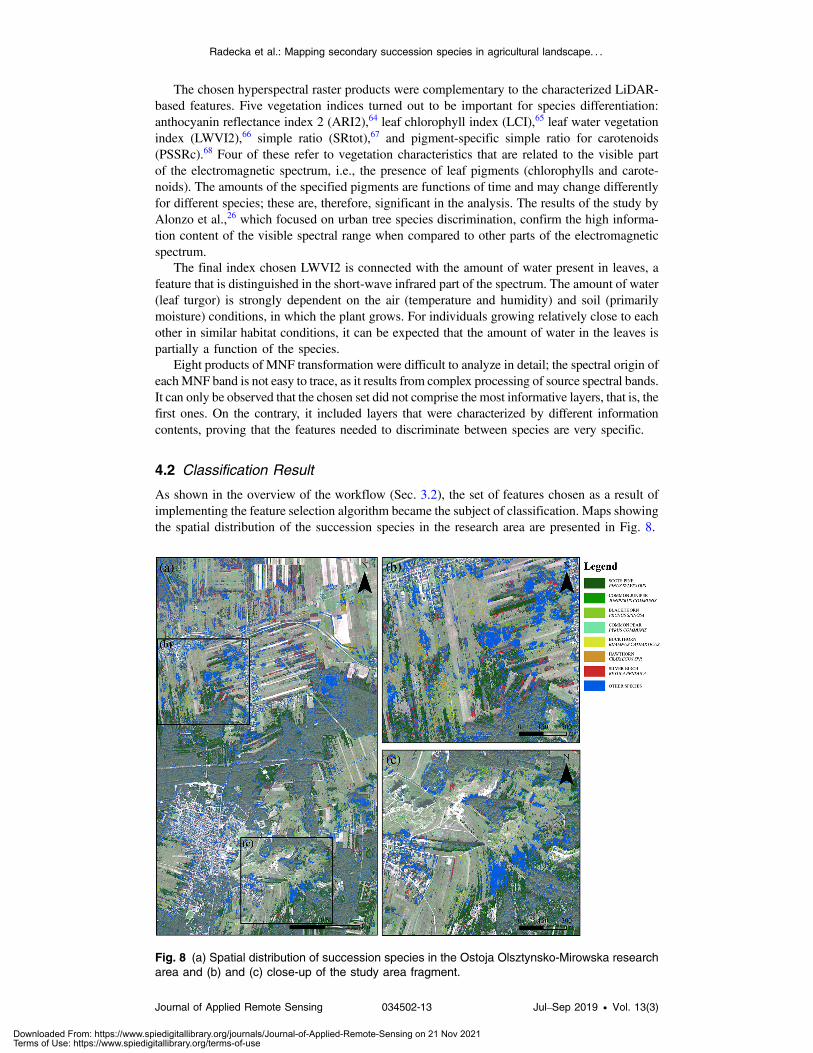
As shown in the overview of the workflow (Sec. 3.2), the set of features chosen as a result ofimplementing the feature selection algorithm became the subject of classification. Maps showingthe spatial distribution of the succession species in the research area are presented in Fig. 8.

Fig. 8 (a) Spatial distribution of succession species in the Ostoja Olsztynsko-Mirowska researcharea and (b) and (c) close-up of the study area fragment.




The maps reveal that the most frequently occurring succession species are Pinus sylvestrisand Betula pendula (mainly in the northern part of the study area). A large part of the researcharea is also occupied by nonsuccessive species, referred to here as “other.” Both of the abovespecies, Pinus sylvestris and Betula pendula, occur in compact single-species patches. In mostcases, Pinus sylvestris is present close to the border between arable land and dense coniferousstands, whereas Betula pendula occurs in various places. The rest of the classified successionspecies do not form regularly shaped patches and are mostly scattered. In general, the trees andshrubs shaping the succession process form elongated patches corresponding to the fallows on orclose to which they grow. This is obvious given that fallows, as unused land, are places withmostly undisturbed ecological processes.

4.3 Accuracy Assessment

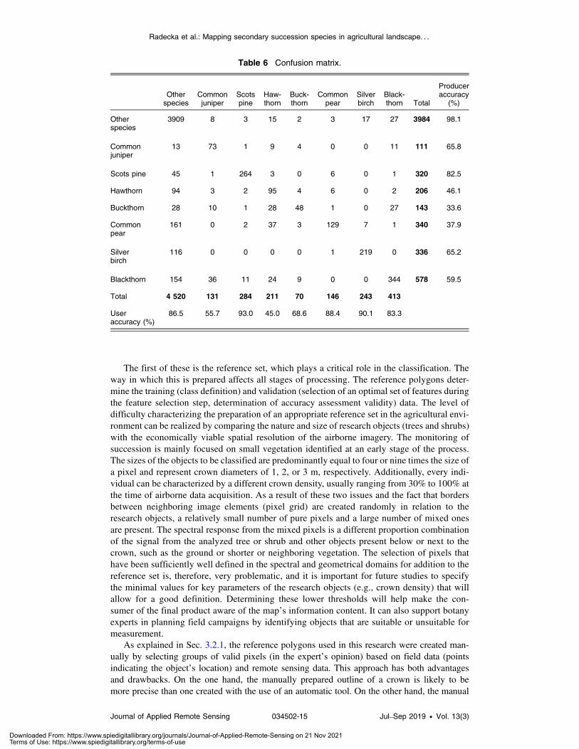
The classification result was evaluated using statistical measures as part of an accuracy assess-ment. The report included the value of Cohen’s kappa, which characterizes the global accuracyof the product; F1 scores, which provide information about the classification accuracy of eachspecies (Table 5); and a confusion matrix (Table 6).

The value of Cohen’s kappa of 0.681 suggests that discrimination between succession spe-cies was relatively successful; however, individual species were classified with various levels ofaccuracy. The highest F1 score of 0.919 characterized the “other” class, which could have beenpredicted in view of the large amount of reference data in the class and the broad range of valuesit encompassed. The confusion matrix indicates that this class had a very low omission error(1.9%) and a higher commission error (13.5%), spreading into other classes, especiallyPyrus communis, Betula pendula, and Prunus spinosa. The same tendencies in the commissionerror of the “other” class were observed by Colgan et al.45 and Graves et al.23

It can also be noticed that three succession species, Betula pendula, Pinus sylvestris, andPrunus spinosa, were classified with high accuracy, with F1 scores of 0.756, 0.874, and0.694, respectively. The four remaining species were classified with average accuracy, rangingfrom F1 ¼ 0.451 for Rhamnus cathartica to F1 ¼ 0.603 for Juniperus communis.

5 Discussion

In this study, a methodology for identifying succession species in an agricultural landscape wasproposed and evaluated. The results obtained here indicate that the selected approach is valid,although there are several points that can be further developed.

Table 5 F1 scores and Cohen’s kappa.

Species name F1 score

Silver birch, Betula pendula 0.756

Scots pine, Pinus sylvestris 0.874

Common juniper, Juniperus communis 0.603

Buckthorn, Rhamnus cathartica 0.451

Hawthorn, Crataegus spp. 0.456

Blackthorn, Prunus spinosa 0.694

Common pear, Pyrus communis 0.531

Other species 0.919

Cohen’s kappa

0.681




The first of these is the reference set, which plays a critical role in the classification. Theway in which this is prepared affects all stages of processing. The reference polygons deter-mine the training (class definition) and validation (selection of an optimal set of features duringthe feature selection step, determination of accuracy assessment validity) data. The level ofdifficulty characterizing the preparation of an appropriate reference set in the agricultural envi-ronment can be realized by comparing the nature and size of research objects (trees and shrubs)with the economically viable spatial resolution of the airborne imagery. The monitoring ofsuccession is mainly focused on small vegetation identified at an early stage of the process.The sizes of the objects to be classified are predominantly equal to four or nine times the size ofa pixel and represent crown diameters of 1, 2, or 3 m, respectively. Additionally, every indi-vidual can be characterized by a different crown density, usually ranging from 30% to 100% atthe time of airborne data acquisition. As a result of these two issues and the fact that bordersbetween neighboring image elements (pixel grid) are created randomly in relation to theresearch objects, a relatively small number of pure pixels and a large number of mixed onesare present. The spectral response from the mixed pixels is a different proportion combinationof the signal from the analyzed tree or shrub and other objects present below or next to thecrown, such as the ground or shorter or neighboring vegetation. The selection of pixels thathave been sufficiently well defined in the spectral and geometrical domains for addition to thereference set is, therefore, very problematic, and it is important for future studies to specifythe minimal values for key parameters of the research objects (e.g., crown density) that willallow for a good definition. Determining these lower thresholds will help make the con-sumer of the final product aware of the map’s information content. It can also support botanyexperts in planning field campaigns by identifying objects that are suitable or unsuitable formeasurement.

As explained in Sec. 3.2.1, the reference polygons used in this research were created man-ually by selecting groups of valid pixels (in the expert’s opinion) based on field data (pointsindicating the object’s location) and remote sensing data. This approach has both advantagesand drawbacks. On the one hand, the manually prepared outline of a crown is likely to bemore precise than one created with the use of an automatic tool. On the other hand, the manual

Table 6 Confusion matrix.

Otherspecies

Commonjuniper

Scotspine

Haw-thorn

Buck-thorn

Commonpear

Silverbirch

Black-thorn Total

Produceraccuracy

(%)

Otherspecies

3909 8 3 15 2 3 17 27 3984 98.1

Commonjuniper

13 73 1 9 4 0 0 11 111 65.8

Scots pine 45 1 264 3 0 6 0 1 320 82.5

Hawthorn 94 3 2 95 4 6 0 2 206 46.1

Buckthorn 28 10 1 28 48 1 0 27 143 33.6

Commonpear

161 0 2 37 3 129 7 1 340 37.9

Silverbirch

116 0 0 0 0 1 219 0 336 65.2

Blackthorn 154 36 11 24 9 0 0 344 578 59.5

Total 4 520 131 284 211 70 146 243 413

Useraccuracy (%)

86.5 55.7 93.0 45.0 68.6 88.4 90.1 83.3




treatment of mixed pixels may be inconsistent between different individuals, while an automatedtool would act in a reliable way and would create an approach that is better fitted to the data.Future research on this subject should be focused on testing different segmentation methods orother automated procedures. The results of research studies by Alonzo et al.,26 Graves et al.,23

Colgan et al.,45 and Shen and Cao28 suggest that these techniques can be used for the correct andefficient delineation of single trees based on the remote sensing data.

The most problematic issue concerning the classification stage seems to be the definition ofclasses. The approach applied in the current work is directly related to the project’s needs: eachsuccession species was treated as a separate class, whereas the rest of the vegetation occurringin the study area was placed in the “other” class. The results of the accuracy assessment suggestthat a few species are very similar to each other, based on remote sensing measures, and thatmerging these should probably be considered in the future. Incorporating an automatic analysisof the separability of the classes into the methodology may be an optimal way of dealing withthis problem. This separability analysis needs to be done individually, not only for differentgroups of species but also for other individuals (due to intraspecies diversity) and obviouslyfor remote sensing data acquisition dates, as a result of the vegetation’s phenological stagesover time.

The postprocessing of the final product is also a challenging task. An image resulting fromthe application of the random forest classifier characterizes each pixel as belonging to a singlechosen class; that is, the research area is entirely classified. The correct delineation of the spatialextent of the species, therefore, requires further processing. This can be done in several differ-ent ways:

• By collecting the reference polygons for each of the classes present in the research area,this may be time-consuming and therefore expensive, especially if the study site is char-acterized by high biodiversity, i.e., a large number of species.

• By creating a special mask, i.e., a layer containing the objects and areas for which a refer-ence was not provided and which are therefore to be deleted from the classification map.This method has been proven to be effective for eliminating objects and areas that arerelatively easy to define, such as anthropogenic areas or water, but is often useless fordeleting nonsuccessive species that are very similar to the research objects.

• Using a measure of similarity between the model (training set) and an analyzed pixel. Thecalculated values can be thresholded to select pixels with low similarity values, i.e., thosethat should not be included in any of the analyzed classes. This is the most straightforwardapproach, but is not always available for a given classifier, for example, the random forestalgorithm used in this research. This problem was also discussed by Alonzo et al.26

• By utilizing a combination of the aforementioned approaches.

As indicated in Sec. 3.2.5, the classification map was postprocessed using a combinedapproach. Different nonvegetative objects and areas were delineated using a special mask, whilepixels representing nonsuccessive species were chosen by creating an “other” class from a selec-tion of representative species. This approach is easy to implement: it does not require any com-plicated calculations and can be applied without collecting a reference for each species.However, it often overestimates the “other” class because of its high variance. The issue of thedefinition of the “other” class should be studied further in the future.

6 Conclusion

The aim of this research was to determine the potential of an accurate identification of successionspecies present in an agricultural landscape with the use of high-resolution aerial remote sensingdata. Promising results were obtained from classifying a dataset comprised of hyperspectral andLiDAR-based products using the random forest algorithm. The use of the RFE algorithm alsoenabled us to observe that both data sources are important in the correct discrimination of spe-cies. The operational use of the methodology presented here requires several elements to bedeveloped further; these are the preparation procedure for the reference polygons and the def-inition of the classes used in classification.




Acknowledgments

The authors would like to express their gratitude to MGGPAero Sp. z o.o. for preprocessing thehyperspectral and LiDAR data and to Justyna Wylazłowska for helping with the botanical fieldcampaign. This research was partially funded by the Poland National Centre for Research andDevelopment. Three types of experts are involved in the project’s implementation: airborneremote sensing data provider (Consortium Leader: company MGGP Aero), botany experts(project partners, scientific units: University of Lodz, Institute of Technology and LifeSciences, and University of Silesia in Katowice), and remote sensing specialists (project part-ners, scientific units: Warsaw University of Technology, University of Warsaw, and WarsawUniversity of Life Sciences). The authors declare no conflict of interest.

References

1. N. Kolecka et al., “Mapping secondary forest succession on abandoned agricultural landwith LiDAR point clouds and terrestrial photography,” Remote Sens. 7, 8300–8322 (2015).

2. M. Szostak et al., “Monitoring the secondary forest succession and land cover/use changesof the Błedów Desert (Poland) using geospatial analyses,” Quaestiones Geographicae35(3), 1–13 (2016).

3. M. Szostak, P. Hawryło, and D. Piela, “Using of Sentinel-2 images for automation of theforest succession detection,” Eur. J. Remote Sens. 51(1), 142–149 (2017).

4. S. Martinuzzi et al., “Quantifying tropical dry forest type and succession: substantialimprovement with LiDAR,” Biotropica 45(2), 135–146 (2013).

5. M. J. Falkowski et al., “Characterizing forest succession with lidar data: an evaluation for theInland Northwest, USA,” Remote Sens. Environ. 113, 946–956 (2009).

6. M. Castillo et al., “LIDAR remote sensing for secondary tropical dry forest identification,”Remote Sens. Environ. 121, 132–143 (2012).

7. M. S. Vanderlinder et al., “Use of remote sensing to assess changes in wetland plant com-munities over an 18-year period: a case study from the Bear River Migratory Bird Refuge,Great Salt Lake, Utah,” West. N. Am. Nat. 74(1), 33–46 (2014).

8. J. A. Gallardo-Cruz et al., “Predicting tropical dry forest successional attributes from space:is the key hidden in image texture?” PLoS One 7(2), e30506 (2012).

9. U. J. Sánchez-Reyes et al., “Assessment of land use-cover changes and successional stagesof vegetation in the natural protected area Altas Cumbres, Northeastern Mexico, usingLandsat satellite imagery,” Remote Sens. 9(7), 712 (2017).

10. M. Batistella and D. Lu, “Integrating field data and remote sensing to identify secondary suc-cession stages in the Amazon,” 2002, https://www.researchgate.net/publication/255609982_Integrating_Field_Data_and_Remote_Sensing_to_Identify_Secondary_Succession_Stages_in_the_Amazon (accessed 15 August 2018).

11. I. C. G. Vieira et al., “Classifying successional forests using Landsat spectral propertiesand ecological characteristics in eastern Amazonia,” Remote Sens. Environ. 87, 470–481(2003).

12. V. E. Garcia-Millan, G. A. Sanchez-Azofeifa, and G. C. Malvárez, “Mapping tropical dryforest succession with CHRIS/PROBA hyperspectral images using nonparametric decisiontrees,” IEEE J. Sel. Top. Appl. Earth Obs. Remote Sens. 8(6), 3081–3094 (2015).

13. G. Çakir et al., “Mapping secondary forest succession with geographic information sys-tems: a case study from Bulanikdere, Kirklareli, Turkey,” Turk J. Agric. For. 31(1), 71–81(2006).

14. B. Barabasz-Krasny, “Vegetation differentiation and secondary succession on abandonedagricultural large-areas in south-eastern Poland,” Biodiv. Res. Conserv. 41, 35–50 (2016).

15. P. Poschlod, J. P. Bakker, and S. Kahmen, “Changing land use and its impact on biodiver-sity,” Basic Appl. Ecol. 6, 93–98 (2005).

16. D. Van der Hoek and K. V. Sykora, “Fen meadow succession in relation to spatial andtemporal differences in hydrology and soil conditions,” Appl. Veg. Sci. 9, 185–194 (2006).

17. Á. J. Albert et al., “Secondary succession in sandy old-fields: a promising example ofspontaneous grassland recovery,” Appl. Veg. Sci. 17, 214–224 (2014).




https://doi.org/10.3390/rs70708300

https://doi.org/10.1515/quageo-2016-0022

https://doi.org/10.1080/22797254.2017.1412272

https://doi.org/10.1111/btp.2013.45.issue-2

https://doi.org/10.1016/j.rse.2009.01.003


https://doi.org/10.3398/064.074.0104

https://doi.org/10.1371/journal.pone.0030506

https://doi.org/10.3390/rs9070712

https://www.researchgate.net/publication/255609982_Integrating_Field_Data_and_Remote_Sensing_to_Identify_Secondary_Succession_Stages_in_the_Amazon






https://doi.org/10.1109/JSTARS.2014.2365180

https://doi.org/10.1515/biorc-2016-0005

https://doi.org/10.1016/j.baae.2004.12.001

https://doi.org/10.1111/j.1654-109X.2006.tb00667.x

https://doi.org/10.1111/avsc.12068

18. Z. Kącki and D. Michalska-Hejduk, “Assessment of biodiversity in Molinia Meadows inKampinoski National Park based on biocenotic indicators,” Polish J. Environ. Stud. 19(2),351–362 (2010).

19. A. Suder, “Purple-moor grass meadows (alliance Molinion caeruleae Koch 1926) in theeastern part of Silesia Upland: phytosociological diversity and aspects of protection,”Nat. Conserv. 65, 63–77 (2008).

20. F. Neves et al., “Successional and seasonal changes in a community of dung beetles (Cole-optera: Scarabaeinae) in a Brazilian tropical dry forest,” Nat. Conserv. 8, 160–164 (2010).

21. M. Quesada et al., “Succession and management of tropical dry forests in the Americas:review and new perspectives,” For. Ecol. Manage. 258, 1014–1024 (2009).

22. J. Tews, “Animal species diversity driven by habitat heterogeneity/diversity: the importanceof keystone structures,” J. Biogeogr. 31, 79–92 (2004).

23. S. J. Graves et al., “Tree species abundance predictions in a tropical agricultural landscapewith a supervised classification model and imbalanced data,” Remote Sens. 8, 161 (2016).

24. N. E. Zimmermann et al., “Remote sensing-based predictors improve distribution models ofrare, early successional and broadleaf tree species in Utah,” J. Appl. Ecol. 44, 1057–1067(2007).

25. C. M. Chance et al., “Invasive shrub mapping in an urban environment from hyperspectraland LiDAR-derived attributes,” Front. Plant Sci. 7, 1–19 (2016).

26. M. Alonzo, B. Bookhagen, and D. A. Roberts, “Urban tree species mapping using hyper-spectral and LIDAR data fusion,” Remote Sens. Environ. 148, 70–83 (2014).

27. L. Liu et al., “Mapping urban tree species using integrated airborne hyperspectral andLiDAR remote sensing data,” Remote Sens. Environ. 200, 170–182 (2017).

28. X. Shen and L. Cao, “Tree-species classification in subtropical forests using airborne hyper-spectral and LiDAR data,” Remote Sens. 9, 1180 (2017).

29. M. Dalponte, L. Bruzzone, and D. Gianelle, “Fusion of hyperspectral and LIDAR remotesensing data for classification of complex forest areas,” IEEE Trans. Geosci. Remote Sens.46(5), 1416–1427 (2008).

30. G. P. Asner et al., “Invasive species detection in Hawaiian rainforests using airborne imagingspectroscopy and LiDAR,” Remote Sens. Environ. 112, 1942–1955 (2008).

31. J. Kondracki, Geografia Regionalna Polski, p. 440, Wydawnictwo Naukowe PWN,Warszawa (1998).

32. M. Ruszkiewicz-Michalska and D. Michalska-Hejduk, “Grzyby pasożytnicze roślin char-akterystycznych dla muraw kserotermicznych Festuco-Brometea w okolicach Olsztyna kołoCzestochowy [Phytopathogenic fungi of characteristic plant species of Festuco-Brometeaxerothermic grasslands in the vicinity of Olsztyn near Czestochowa],” ZiemiaCzestochowska 30, 195–208 (2003).

33. “Standard data form for Natura 2000 site PLH240015,” Olsztyńsko-Mirowska Refuge,http://n2k-ws.gdos.gov.pl/wyszukiwarkaN2k/webresources/pdf/PLH240015 (accessed 22January 2018).

34. J. A. M. Janssen and J. Dengler, “E1.9a oceanic to subcontinental inland sand grassland ondry acid and neutral soils,” European Red List of Habitats—Grasslands Habitat Group,https://www.researchgate.net/publication/312297575_E19a_Oceanic_to_subcontinental_inland_sand_grassland_on_dry_acid_and_neutral_soils (accessed 31 May 2017).

35. B. Calaciura and O. Spinelli, “Management of Natura 2000 habitats. 6210 Seminatural drygrasslands and land facies on calcareous substrates (Festuco-Brometalia) (*important orchidsites),” European Commission. Technical Report 12(24) (2008).

36. M. F. W. DeVries, P. Poschlod, and J. H. Willems, “Challenges for the conservation ofcalcareous grasslands in Northwestern Europe: integrating the requirements of flora andfauna,” Biol. Conserv. 104, 265–273 (2002).

37. The Convention on the Conservation of European Wildlife and Natural Habitats, EuropeanTreaty Series 104, Join Nature Conservation Committee, Peterborough, https://rm.coe.int/1680078aff (accessed 22 January 2018).

38. W. Mróz, Monitoring siedlisk przyrodniczych. Przewodnik metodyczny [Natura 2000Habitat Monitoring], Part I–III, Biblioteka Monitoringu Środowiska, Warszawa, Poland(2010–2012).




https://doi.org/10.4322/natcon.00802009

https://doi.org/10.1016/j.foreco.2009.06.023

https://doi.org/10.1046/j.0305-0270.2003.00994.x

https://doi.org/10.3390/rs8020161

https://doi.org/10.1111/jpe.2007.44.issue-5

https://doi.org/10.3389/fpls.2016.01528



https://doi.org/10.3390/rs9111180

https://doi.org/10.1109/TGRS.2008.916480


http://n2k-ws.gdos.gov.pl/wyszukiwarkaN2k/webresources/pdf/PLH240015




https://www.researchgate.net/publication/312297575_E19a_Oceanic_to_subcontinental_inland_sand_grassland_on_dry_acid_and_neutral_soils




https://doi.org/10.1016/S0006-3207(01)00191-4

https://rm.coe.int/1680078aff




39. S. Colas and M. Hébert, “Guide d’estimation des coûts de gestion des milieux naturelsouverts,” [Guide for estimating the costs of managing open natural environments],Espaces Naturels de France (2000).

40. Habitats Directive Annex I Habitats, European Commission, Interpretation Manual ofEuropean Union Habitats, version EUR 28, 2013, http://ec.europa.eu/environment/nature/legislation/habitatsdirective/docs/Int_Manual_EU28.pdf (accessed 22 January 2018).

41. M. Partel et al., “Restoration of species-rich limestone grassland communities from over-grown land: the importance of propagule availability,” Ecol. Eng. 10, 275–286 (1998).

42. The Invertebrate Conservation Trust, “Advice on managing BAP habitats,” UplandCalcareous Grassland, 2007, https://www.buglife.org.uk/advice-and-publications/advice-on-managing-bap-habitats/upland-calcareous-grassland (accessed 22 January 2018).

43. “HySpex products,” https://www.hyspex.no/products/ (accessed 22 February 2018).44. “Datasheet Riegl LMS-Q680i,” 2012, http://www.riegl.com/uploads/tx_pxpriegldownloads/

10_DataSheet_LMS-Q680i_28-09-2012_01.pdf (accessed 22 January 2018).45. M. S. Colgan et al., “Mapping savanna tree species at ecosystem scales using support vector

machine classification and BRDF correction on airborne hyperspectral and LiDAR data,”Remote Sens. 4, 3462–3480 (2012).

46. RiProcess Data Sheet for RIEGL Scan Data, http://www.riegl.com/uploads/tx_pxpriegldownloads/11_Datasheet_RiProcess_2016-09-16_01.pdf (20 September 2018).

47. RiAnalyze Data Sheet for Automated Resolution of Range Ambiguities, http://www.riegl.com/uploads/tx_pxpriegldownloads/11_DataSheet_RiMTA-ALS_2015-08-24_03.pdf(accessed 20 September 2018).

48. P. Axelsson, “Processing of laser scanner data-algorithms and applications,” ISPRS J.Photogramm. Remote Sens. 54(2), 138–147 (1999).

49. “TerraSolid Terrascan user guide,” http://www.terrasolid.com/guides/tscan/index.html(accessed 20 July 2018).

50. G. Mandlburger et al., “OPALS—a comprehensive laser scanning software for geomorpho-logical analysis,” inGeophys. Res. Abstr., Vol. 13, EGU2011-7933, EGU General Assembly(2011).

51. B. Höfle et al., “Detection of building regions using airborne LiDAR: a new combination ofraster and point cloud based GIS methods,” in Proc. GI-Forum—Int. Conf. Appl. Geoinf.,Salzburg, Austria, pp. 66–75 (2009).

52. BCAL, BCAL Lidar Tools, Boise, Idaho, 2016, https://bcal.boisestate.edu/tools/lidar(accessed 22 January 2018).

53. J. S. Evans et al., “Discrete return Lidar in natural resources: recommendations for projectplanning, data processing, and deliverables,” Remote Sens. 1(4), 776–794 (2009).

54. HySpex RAD, https://www.hyspex.no/ (accessed 26 October 2018).55. D. Schläpfer, “Parametric Geocoding, PARGE User Guide, Version 3.3, ReSe Applications

Schläpfer, p. 270 (2016).56. R. Richter and D. Schlapfer, “ATCOR4 manual,” ReSe Applications, https://www.rese-apps

.com/pdf/atcor4_manual.pdf (accessed 26 October 2018).57. Ł. Sławik et al., “Multiple flights or single flight instrument fusion of hyperspectral and ALS

data? A comparison of their performance for vegetation mapping,” Remote Sens. 11, 970(2019).

58. A. A. Green et al., “A transformation for ordering multispectral data in terms of image qual-ity with implications for noise removal,” IEEE Trans. Geosci. Remote Sens. 26(1), 65–74(1988).

59. “ENVI API programming guide,” Harris Geospatial Solutions Documentation Center,http://www.harrisgeospatial.com/docs/ProgrammingGuideIntroduction.html (accessed 21September 2018).

60. A. Rabe et al., “EnMAP-Box 3 documentation,” Earth Observation Center EOC of DLR,Germany, http://www.enmap.org/enmapbox.html (accessed 12 December 2018).

61. R. Archibald and G. Fann, “Feature selection and classification of hyperspectral imageswith support vector machines,” IEEE Geosci. Remote Sens. Lett. 4(4), 674–677 (2007).

62. A. A. G. Singh, A. Balamurugan, and J. Leavline, “Literature review on feature selectionmethods for high-dimensional data,” Int. J. Comput. Appl. 136(1), 9–17 (2016).




http://ec.europa.eu/environment/nature/legislation/habitatsdirective/docs/Int_Manual_EU28.pdf





https://doi.org/10.1016/S0925-8574(98)00014-7

https://www.buglife.org.uk/advice-and-publications/advice-on-managing-bap-habitats/upland-calcareous-grassland





https://www.hyspex.no/products/



http://www.riegl.com/uploads/tx_pxpriegldownloads/10_DataSheet_LMS-Q680i_28-09-2012_01.pdf





https://doi.org/10.3390/rs4113462

http://www.riegl.com/uploads/tx_pxpriegldownloads/11_Datasheet_RiProcess_2016-09-16_01.pdf





http://www.riegl.com/uploads/tx_pxpriegldownloads/11_DataSheet_RiMTA-ALS_2015-08-24_03.pdf




https://doi.org/10.1016/S0924-2716(99)00008-8

https://doi.org/10.1016/S0924-2716(99)00008-8

http://www.terrasolid.com/guides/tscan/index.html




https://bcal.boisestate.edu/tools/lidar



https://doi.org/10.3390/rs1040776

https://www.hyspex.no/



https://www.rese-apps.com/pdf/atcor4_manual.pdf




https://doi.org/10.3390/rs11080970

https://doi.org/10.1109/36.3001

http://www.harrisgeospatial.com/docs/ProgrammingGuideIntroduction.html




http://www.enmap.org/enmapbox.html




https://doi.org/10.1109/LGRS.2007.905116

https://doi.org/10.5120/ijca2016908317

63. R. G. Congalton and K. Green, Assessing the Accuracy of Remotely Sensed Data: Principlesand Practices, CRC Press, Taylor & Francis Group, Boca Raton (2008).

64. A. A. Gitelson, M. N. Merzlyak, and O. B. Chivkunova, “Optical properties and non-destructive estimation of anthocyanin content in plant leaves,” Photochem. Photobiol.74(1), 38–45 (2001).

65. B. Datt, “A new reflectance index for remote sensing of chlorophyll content in higher plants:tests using eucalyptus leaves,” J. Plant Physiol. 154, 30–36 (1999).

66. L. S. Galvao, A. R. Formaggio, and D. A. Tisot, “Discrimination of sugarcane varieties inSoutheastern Brazil with EO-1 Hyperion data,” Remote Sens. Environ. 94(4), 523–534(2005).

67. B. Datt, “Remote sensing of chlorophyll a, chlorophyll b, chlorophyll a+b and total carot-enoid content in eucalyptus leaves,” Remote Sens. Environ. 66, 111–121 (1998).

68. G. A. Blackburn, “Spectral indices for estimating photosynthetic pigment concentration: atest using senescent tree leaves,” Int. J. Remote Sens. 19(4), 657–675 (1998).

Aleksandra Radecka received her BSc and MSc degrees in spatial planning from WarsawUniversity of Technology (WUT) in Poland, in 2015 and 2017, respectively. She is currentlypursuing her PhD in geodesy and cartography at WUT. Since 2016, she has worked as a researchassistant in the Department of Photogrammetry, Remote Sensing and Spatial InformationSystems, WUT. Her research interest includes the usage of thermal and hyperspectral remotesensing techniques for environmental studies.

Dorota Michalska-Hejduk received her MSc degree in biology and her PhD in ecology fromthe University of Lodz in Poland where she is working in the Department of Geobotany andPlant Ecology. Her research interests include plant science, nature protection, monitoring ofNatura 2000 habitats and species, and ecological processes. In 2014, she received an award forservices to “Environmental Protection and Water Management” from the Ministry of theEnvironment in Poland. She is a member of the Society of Ecological Restoration.

Katarzyna Osińska-Skotak received her MSc degree in photogrammetry and cartography in1994, her MSc degree in meteorology and atmosphere protection in 1997, her PhD in 2001, andher DSc degree in photogrammetry and remote sensing in 2011 from Warsaw University ofTechnology (WUT) in Poland. Since 2012, she has been a head of the Department ofPhotogrammetry, Remote Sensing and Spatial Information Systems at WUT. Her research inter-ests include the applications of thermal, multi- and hyperspectral remote sensing techniques inenvironmental and urban monitoring. She is a board member of the Remote Sensing andGeoinformatics Group of the Polish Geographical Society.

Adam Kania has experience in private consultancy for business in areas such as environmentalmanagement, quality management systems, IT management, and software development. Hisareas of interest also included data processing, statistics, machine learning, optimization, andAI algorithms. He is currently leading the development of the Vegetation ClassificationStudio—a scientific software tool for fast and effective classification of remote sensing data.Last year, he founded Definity Ltd., a company working in research and development of algo-rithms and tools for AI, machine learning, remote sensing, and scientific computing.

Konrad Górski received his MSc degree in photogrammetry and remote sensing in 2016 fromWarsaw University of Technology (WUT) in Poland. He is now a PhD student at the WUTFaculty of Geodesy and Cartography. From 2016 to 2018, he has been working in theDepartment of Photogrammetry, Remote Sensing and Spatial Information Systems at WUT.His research interests include employing new sensors and processing techniques in a wide rangeof specialized applications, especially modern ultralight sensors compatible with unmannedplatforms, to enhance industry capabilities.

Wojciech Ostrowski received his MSc degree in geodesy and cartography (specialization:photogrammetry and remote sensing) in 2013 from Warsaw University of Technology (WUT)in Poland, where he has been working as a research-teaching assistant in the Department of




https://doi.org/10.1562/0031-8655(2001)074%3C0038:OPANEO%3E2.0.CO;2

https://doi.org/10.1016/S0176-1617(99)80314-9


https://doi.org/10.1016/S0034-4257(98)00046-7

https://doi.org/10.1080/014311698215919

Photogrammetry, Remote Sensing and Spatial Information Systems, since 2013. His researchinterests include LIDAR data applications in archaeology prospection and remote sensing aswell as photogrammetric processing of UAV and aerial oblique images. He is a member of thePolish Society for Photogrammetry and Remote Sensing, and the Computer Applications andQuantitative Methods in Archaeology and Aerial Archaeology Research Group.




mapping secondary succession species in agricultural

Documents