arX

iv:a

stro

-ph/

9710

327v

2 1

0 Fe

b 19

98

Maps of Dust IR Emission for Use in Estimation of Reddening

and CMBR Foregrounds

David J. Schlegel

University of Durham, Department of Physics, South Road, Durham DH1 3LE, United

Kingdom

and

Douglas P. Finkbeiner & Marc Davis

University of California at Berkeley, Departments of Physics and Astronomy, 601 Campbell

Hall, Berkeley, CA 94720

ABSTRACT

We present a full sky 100µm map that is a reprocessed composite of

the COBE/DIRBE and IRAS/ISSA maps, with the zodiacal foreground and

confirmed point sources removed. Before using the ISSA maps, we remove the

remaining artifacts from the IRAS scan pattern. Using the DIRBE 100µm and

240µm data, we have constructed a map of the dust temperature, so that the

100µm map may be converted to a map proportional to dust column density.

The dust temperature varies from 17 K to 21 K, which is modest but does

modify the estimate of the dust column by a factor of 5. The result of these

manipulations is a map with DIRBE-quality calibration and IRAS resolution. A

wealth of filamentary detail is apparent on many different scales at all Galactic

latitudes. In high latitude regions, the dust map correlates well with maps of H I

emission, but deviations are coherent in the sky and are especially conspicuous

in regions of saturation of H I emission toward denser clouds and the formation

of H2 in molecular clouds. In contrast, high-velocity H I clouds are deficient in

dust emission, as expected.

To generate the full sky dust maps, we must first remove zodiacal light

contamination as well as a possible cosmic infrared background (CIB). This

is done via a regression analysis of the 100µm DIRBE map against the

Leiden-Dwingeloo map of H I emission, with corrections for the zodiacal light

via a suitable expansion of the DIRBE 25µm flux. This procedure removes

virtually all traces of the zodiacal foreground. For the 100µm map no significant

CIB is detected. At longer wavelengths, where the zodiacal contamination is

weaker, we detect the CIB at surprisingly high flux levels of 32 ± 13 nW/m2/sr

– 2 –

at 140µm, and 17 ± 4 nW/m2/sr at 240µm (95% confidence). This integrated

flux is ∼ 2 times that extrapolated from optical galaxies in the Hubble Deep

Field.

The primary use of these maps is likely to be as a new estimator of Galactic

extinction. To calibrate our maps, we assume a standard reddening law, and use

the colors of elliptical galaxies to measure the reddening per unit flux density

of 100µm emission. We find consistent calibration using the (B−R) color

distribution of a sample of 106 brightest cluster ellipticals, as well as a sample of

384 ellipticals with (B−V ) and Mg line-strength measurements. For the latter

sample, we use the correlation of intrinsic (B−V ) versus Mg2 index to greatly

tighten the power of the test. We demonstrate that the new maps are twice as

accurate as the older Burstein-Heiles reddening estimates in regions of low and

moderate reddening. The maps are expected to be significantly more accurate

in regions of high reddening. These dust maps will also be useful for estimating

millimeter emission that contaminates CMBR experiments and for estimating

soft X-ray absorption.

We describe how to readily access our maps for general use.

Subject headings: Cosmology: observations — dust — extinction — infrared:

ISM: continuum

1. Introduction

In the past 15 years, two NASA missions have revolutionized our knowledge of the

diffuse interstellar medium. The path-breaking Infrared Astronomy Satellite (IRAS) mission

of 1983 led to the first full-sky maps of the diffuse background radiation in four broadband

infrared channels, centered at 12, 25, 60, and 100µm, with a ∼ 5 arcminute beam. The

DIRBE experiment (Diffuse InfraRed Background Experiment) onboard the COBE satellite

imaged the full sky in 10 broad photometric bands from 1µm to 240µm with a beam of

0.7. This experiment, for all but the shortest wavelength channels, was active for 42

weeks in 1989-1990 before its 4He cryogen was exhausted. Although IRAS was optimized

to detect point sources and sources of small angular extent (Beichman et al. 1988), it has

been possible to create large area sky maps from the IRAS data stream (ISSA images:

Wheelock et al. 1994). Striping artifacts from time variation in the zodiacal foreground

emission has largely been filtered out of the individual ISSA maps, but artifacts remain and

the zero-point has large-scale drifts across the images. The DIRBE experiment had a much

– 3 –

better control of the absolute calibration and has two channels further to the submillimeter

than does IRAS (at 140µm and 240µm), but the maps have much less angular resolution.

The diffuse emission seen in these experiments is a superposition of zodiacal foreground

emission, dust and molecular emission from the interstellar medium (ISM), point sources

from within and beyond the Milky Way, and possibly a diffuse extragalactic background.

Separating these components has proven to be a most difficult task (Hauser 1996).

The zodiacal emission dominates the 12µm and 25µm channels and is a quite serious

contaminant at 60µm, while its contribution to the 100µm maps is less strong. Modelling

of the zodiacal emission has proven quite complex (Reach et al. 1996). One must consider

that the zodiacal dust in the ecliptic plane has a distribution of temperatures, that the tilt

of Earth’s orbit relative to the midplane of the dust is readily detectable, and that the

zodiacal emission shows a strong dependence on solar elongation, information which is lost

if one uses only the annual-averaged map of the DIRBE data.

A full-sky map of the diffuse radiation serves many purposes, and we here report

our efforts to combine the 100µm maps of IRAS and DIRBE in a manner designed to be

accessible to the general astrophysical community. To construct this map, we have removed

the zodiacal foreground emission from the DIRBE maps, removed striping artifacts from

the IRAS/ISSA maps, subtracted confirmed point sources, and combined the maps in such

a way as to preserve the DIRBE calibration and IRAS resolution. We have used the ratio of

100µm to 240µm emission to deduce a dust color temperature, allowing us to translate the

100µm emission to a column density of radiating dust. Such a procedure may be inadequate

towards complex, dense clouds at low Galactic latitude, but in most directions the emission

is dominated by dust within a single environment and radiation field.

Since the diffuse emission in the infrared is a direct measure of the column density of

the interstellar dust, such a map can be used as a measure of extinction for extragalactic

objects. As we shall argue below, the new dust map has better angular resolution and better

control of systematics than possible with the reddening maps of Burstein & Heiles (1978,

1982). The essence of the Burstein-Heiles procedure was to assume that variations in the

dust-to-neutral-gas ratio can be adequately modelled by the smoothed mean background of

galaxies (at northern declinations), or that this ratio is constant (at southern declinations).

We make no assumptions about variations in dust-to-gas; neither do we need make any

assumption about the correlation of diffuse ionized gas with neutral hydrogen. We only

make the weaker assumption that the distribution of dust grain sizes is everywhere the

same, since the relationship between UV/optical extinction and far-IR emission depends on

the grain size distribution (Draine & Lee 1984; Draine & Anderson 1985; Guhathakurta &

Draine 1989; Mathis & Cardelli 1992). The diffuse gas, where our results apply, is thought

– 4 –

to have reasonably uniform dust properties, with values of RV ≡ A(V )/E(B−V ) ≈ 3.1.

Since neither the Burstein-Heiles nor our assumptions are true for all environments, a

comparison between the different methods is of interest.

To calibrate the extinction curve, we extensively explored the anticorrelation of counts-

in-cells of the APM galaxy survey (Maddox et al. 1990b, 1990c) with 100µm emission,

finding a consistent calibration in different directions of the sky. Due to complications in

translating this calibration into E(B−V ), we shall defer this discussion for a separate paper

(Finkbeiner et al. 1997).

Since we find that the 100µm maps are well correlated with H I emission at high

latitudes, we do not not expect the new extinction maps to grossly deviate from the

Burstein-Heiles reddening estimates when averaged to the same scales. But many dusty

regions have filamentary structure with large fluctuations in extinction estimates over

angular scales much smaller than the resolution of the BH maps. Furthermore, at low

Galactic latitudes, regions such as Orion and Ophiuchus might be saturated in H I emission,

or partially ionized, whereas the dust remains optically thin.

Another important application for maps of the diffuse emission is to compare with

CMBR fluctuation maps. Recent analyses of the COBE/DMR fluctuations (Kogut et al.

1996) show a positive correlation with DIRBE maps, particularly in the North Polar Spur

region. Similar correlations are seen between the Saskatoon CMBR maps and the IRAS

maps (Oliveira et al. 1997; Leitch et al. 1997; Jaffe et al. 1997). This is unexpected, since

these 40 GHz CMBR experiments are not sensitive to dust emission, but are sensitive to

free-free emission from the Warm Ionized Medium (WIM). This implies that the WIM

is at least partly correlated with the cold, dusty medium, and that our dust maps could

be used as a model for both components (Reynolds 1995). Alternatively, the observed

CMBR correlations might be explained by small spinning dust grains producing continuum

emission in the 10− 100 GHz range (Draine & Lazarian 1997), in which case the dust maps

should correlate extremely well with CMBR observations over the entire sky.

This paper is organized as follows: Section 2 describes the processing of the DIRBE

data. We describe how the weekly averaged DIRBE maps are trimmed and then

reconstituted into annual average maps more suitable for our simple treatment of the

zodiacal light removal. We fit a zodiacal light model by maximizing the correlation between

the DIRBE maps and H I in regions of high Galactic latitude and low flux.

The diffuse cirrus emission is expected to have a reasonably uniform temperature since

the ultraviolet radiation field which is heating the dust must be a smooth function of

angular position except within dense clouds. Fortunately, the emission at 100 and 240µm

– 5 –

is expected to be dominated by grains sufficiently large to be in equilibrium with the

radiation field (e.g. Draine & Anderson 1985; Guhathakurta & Draine 1989), so that the

100µm/240µm color ratio can provide a useful measure of grain temperature. In Section

2.4, we describe how we measure the temperature in the presence of substantial noise in

the 240µm map. This information is used to translate the 100µm emission to dust column

density.

The inclusion of the IRAS data is discussed in Section 3. Before we can combine the

IRAS/ISSA map with the DIRBE map, we must first deal with the ISSA boundaries and

discontinuities. The ISSA maps are destriped versions of the original IRAS scans, but

further destriping is possible and essential for high angular-resolution studies. We use a

matched set of window functions that low-pass filter the DIRBE map to 1 resolution and

high-pass filter IRAS/ISSA maps on the same scale. The combined map is then simply the

sum of these two filtered maps. Section 4 details the removal of extragalactic objects and

point sources from the maps, leaving behind only a map of the dust emission.

In Section 5, we present a simple procedure for normalizing the reddening per unit flux

density of dust emission. We correlate the residual of the (B−V ) vs. Mg2 index for 384

elliptical galaxies against the estimated reddening, and adjust the normalization until the

slope of the relation is zero. The resulting calibration has an uncertainty of only 10%. We

also show that the maps have an accuracy of 16% in predicting reddening, which is twice as

good as the older BH procedure.

A summary of all these reprocessing procedures in presented in Section 6. Readers

uninterested in the details of the analysis should skip directly to this point. General

discussion and conclusions are presented in Sections 7 and 8. Appendix A discusses the

contamination level of stars that remain in the maps. Appendix B describes how to relate

the reddenings and extinction in different optical and infrared filters. Appendix C describes

how to access the final maps.

2. Dust Column Densities From the DIRBE Maps

2.1. The DIRBE Data Set

The DIRBE data set is in the public domain and was obtained from the National

Space Science Data Center (NSSDC) on CDROM. For a complete description of the

DIRBE instrument, see Boggess et al. (1992). Both Annual Average Skymaps and maps

averaged over each week of the mission are provided. The data are binned to 393,216

0.32 × 0.32 pixels on the COBE Quadrilateralized Spherical Cube. (For a description of

– 6 –

this “skycube” projection, see Chan & O’Neill 1975.) As described below, we create new

annual average 25µm and 100µm skymaps from the 41 weekly maps in skycube format

in which the weighting function of each week is forced to be the same for both channels.

We then reproject the data to standard, equal-area, polar projections oversampled to 512

pixels from b = 0 to b = 90 (0.0250 square degrees/pixel). In order to preserve total flux

to a good approximation, we initially projected to a Lambert (polar) mapping with 4 × 4

smaller pixels which were then binned to the 0.0250 square-degree resolution. (Note that

the surface brightness of the cirrus is preserved in this re-projection.) These maps for each

passband, b, are denoted by Db, and are in units of MJy/sr. We use the 25µm map as a

model of the zodiacal light, and the 100µm and 240µm maps for measuring the temperature

and column density of the dust.

2.2. Zodiacal Light Removal

The DIRBE maps are severely contaminated by zodiacal emission from dust in the

solar system, otherwise known as the IPD (inter-planetary dust). The IPD primarily

re-radiates thermally at ∼ 280 K in the infrared (for ν0 emissivity). Its emission per unit

column density is substantially higher than that of 20 K Galactic dust: using an α = 2

emissivity law, the 100µm emission of the IPD is larger by a factor ∼ 105 than that of

Galactic dust for an equivalent column density. The brightest zodiacal emission is in the

ecliptic plane, at the level of ∼ 10 MJy/sr. Based upon our solutions, this corresponds to

an extinction at the negligible level of A(B) ≈ 10−6 mag. Thus, the removal of zodiacal

light emission is critical as it makes no measurable contribution to optical extinction.

The 25µm maps, where the IPD emission peaks, is used to model the IPD contamination

at the longer wavelengths. Before removing this contamination, the DIRBE annual average

data must first be regenerated so that the data at all wavelengths are sampled at the

same time and through the same IPD. The zero-points of the zodiacal contamination are

constrained by H I maps at high Galactic latitude.

2.2.1. Dependence on Time and Solar Elongation Angle

Removal of the zodiacal light is a difficult problem. The observing strategy of the

COBE satellite resulted in a lower signal-to-noise ratio in the ecliptic plane where the

zodiacal light is most prominent. The number of high-quality DIRBE observations per

pixel ranged from ∼ 200 at the ecliptic equator to ∼ 800 near the ecliptic poles. The

– 7 –

least-sampled regions were approximately cones of 90 opening angle centered at ecliptic

(λ, β) = (100, 0), and (λ, β) = (280, 0). The DIRBE maps exhibit a striping pattern

perpendicular to the ecliptic plane; scans adjacent in the sky correspond to temporally

separated instrument tracks, taken at varying solar elongation angles, through different

column densities of IPD.

Measurements for each week of the mission were used to construct weekly skymaps.

The DIRBE Annual Average Skymaps are a combination of the weekly maps, averaged

by the number of times that each pixel was observed in a weekly map. Unfortunately, the

whole sky is not scanned each week, and some parts of the scanned region are omitted in

certain weeks due to interference from the moon and planets. Furthermore, not all the

detectors were on at all times.

A cursory glance at the weekly skymaps reveals a serious problem with combining data

in this way. Near the ecliptic plane, the 25µm flux exhibits a strong dependence on solar

elongation angle, e. During the 41 weeks, data were typically taken between e = 64 and

e = 124, and the 25µm flux varies by a factor of two over this range. Comparison with the

100µm IPD flux also reveals a strong temperature gradient with respect to e. This is easily

explained by assuming a radial gradient of IPD density from the sun, because a line of sight

passing close to the sun must traverse more (and hotter) dust than a line of sight at larger

solar elongation. As a further complication, because the 10 passbands were not always

observed simultaneously, the weekly skymaps of the weighting function do not always match

across all channels. Contributions to the Annual Average Skymaps were weighted according

to the number of observations made in each channel, in spite of the strong dependence on

elongation angle.

In cases where the measurement noise is overwhelmed by the time-dependent systematic

variations, this method of averaging is inappropriate. The weights assigned to sky pixels

are thus not always the same for the 25µm and 100µm weekly maps, leading to weighted

Annual Average Skymaps which cannot be directly compared to each other. To rectify

this, we recombine the 41 weekly skymaps using the same weight for the same pixels in

different passbands. We use the error maps for the 100µm passband as weights in all other

passbands. Because the IPD temperature gradient is strongest at low e, we further delete

all data in each weekly map taken at e < 80. The resulting maps have noise and artifacts

which are somewhat worse than the Annual Average Skymaps from the NSSDC; however,

the artifacts are the same at both wavelengths. The resulting 25µm map is appropriate for

modelling the IPD contamination at other wavelengths.

– 8 –

2.2.2. Scale and Zero-Point of the Zodiacal Light

The spatial-temporal variations of zodiacal light are complicated and difficult to model

analytically. Our procedure for removing the zodiacal light assumes that the 100µm map

correlates linearly with H I at high Galactic latitudes and low flux levels (Boulanger et al.

1996). Note that one should also expect some dust within the extensive ionized H+ zones,

and that the column density ratio N(H+)/N(H I) has considerable scatter in different

directions (Reynolds 1990). The relationship between the diffuse ionized and neutral

hydrogen in any direction is complex (Reynolds 1995); some of the H+ is associated with

neutral gas, while other ionized clouds adjoin neutral regions. We are of course interested in

measuring the dust associated with both components, and to the degree that there is dust

within H+ regions not associated with neutral regions, the scatter of dust and H I will be

increased. The degree of scatter between neutral gas and dust is therefore of considerable

interest, but this scatter should not bias our procedure.

We consider the 25µm map as a template of the unwanted zodiacal foreground, as the

25µm channel is so thoroughly dominated by the IPD. In a few regions where the Galactic

cirrus contributes more than a few per cent to the 25µm emission, we interpolate the 25µm

map in bins of constant ecliptic latitude. To first order, we subtract scaled versions of the

25µm map in order to minimize the scatter between the H I and zodiacal-corrected 100µm

and 240µm emission. We further refine this correction with the addition of a quadratic

term to account for temperature variations in the IPD.

Fitting black-body functions to the zodiacal light from 12µm to 60µm, we find that

the color temperature does not vary by more than ten percent from ecliptic equator to the

poles. This allows us to make a first-order correction under the assumption that the IPD

is at a constant temperature. The DIRBE 25µm map, D25, is directly scaled to model

the zodiacal contamination at longer wavelengths. The raw maps for these other DIRBE

passbands, Db, are corrected to

DLb = Db − AbD25 − Bb. (1)

The coefficient Ab determines the scaling of the zodiacal emission from the 25µm DIRBE

passband to passband b. The zero-point offset, Bb, is used to account for a multitude

of non-zodiacal contributions to the 25µm and 100µm maps, either from the Galaxy or

extragalactic light. Although the 25µm map is relatively free of point sources, the ten

brightest sources have been masked to their local averages (see Table 1). Note that these

sources were not excluded from the 100µm or 240µm maps.

Assuming that H I correlates linearly with dust at high latitudes and low flux

levels, we make use of the H I flux to determine the zodiacal flux scaling coefficients and

– 9 –

zero-point offsets. We compare the emission, DL, to the H I column density, H, from

the Leiden-Dwingeloo 21-cm survey (Hartmann & Burton 1996). The 21-cm emission is

summed in the velocity range −72 < vLSR < +25 km/s, which samples almost all of the

Galactic H I at high Galactic latitudes. (At high latitudes, H I outside of this range shows

no correlation with the 100µm maps). We solve for the coefficients Ab and Bb of equation 1

and the H I-to-DIRBE ratio, ζb, using a least-squares minimization of

χ2 =∑

i

[

ζb(DLb )i − Hi

σi

]2

(2)

in each passband. The errors in this relation are systematic and difficult to express

analytically. Therefore, we take the uncertainties, σi, to be proportional to the H I flux.

The fitting procedure is performed on the maps binned to 2.5 and limited to those areas

of the sky with low emission, H I < 200 K km/s, or N(H) < 3.7 × 1018 cm−2 (19% of the

sky). Two dust clouds with unusual temperature and the region immediately around the

very bright source NGC 253 are omitted from the fits. The results of these fits for b = 100,

140, 240µm are presented in Table 2, and a scatter diagram is shown in Figure 1 both (a)

before and (b) after the correction.

Temperature variations in the IPD make the linear correction of equation 1 inadequate

for our purposes. Based on 12µm/25µm and 25µm/60µm ratios, the color temperature of

the IPD varies by 5% for an α = 1 emissivity law or by 10% for an α = 2 emissivity law.

Because the 100µm band is on the Rayleigh-Jeans side of the spectrum, this results in a 5 or

10% error in zodiacal light. As the zodiacal light contributes up to 10 MJy/sr at 100µm in

the ecliptic plane, this results in absolute errors of 1 MJy/sr, with a strong ecliptic latitude

dependence. A constant temperature, linear model of zodiacal dust removal is a good first

approximation, but is clearly too simplistic. Because the neighboring passbands at 12µm

and 60µm are a complex mix of zodiacal and non-zodiacal contributions, it is desirable to

model the variation in IPD temperature using only the 25µm map rather than some linear

combination of passbands. Thus we are driven to higher order fits using only the 25µm

map.

The temperature variations in the IPD are most strongly a function of ecliptic latitude,

β. An adequate second-order function for modelling the variations in IPD emission at

longer wavelengths is to include a term that is linear in the product of D25 and D25(β),

the mean 25µm emission at each ecliptic latitude (limited to |b| > 20 to minimize Galactic

contamination in the model). With a scaling coefficient, Qb, the corrected maps then

become

DQb = Db − (Ab + QbD25(β))D25 − Bb. (3)

The above is referred to as the quadratic correction. Solutions are again found via equation

– 10 –

2 using the same region of the sky as before. Results are presented in Table 2. Since

the linear and quadratic contributions are not orthogonal, there is no particular physical

meaning to the coefficients derived in the quadratic fits; they are merely the coefficients

which yield the minimum χ2.

The result of the quadratic correction is shown in Figure 1(c). At 100µm, the quadratic

correction is clearly superior to the linear correction, reducing the RMS scatter from 19%

to 16% (for H I< 200 K km/s). At 240µm, the difference between the two fits is negligible.

This is both because the 240µm map has a higher inherent noise, and because the zodiacal

light correction at such long wavelengths is smaller. Even though there is no obvious

difference in fitting methods at 240µm, we apply the quadratic correction to both passbands

to avoid introducing systematic errors into the determination of the dust temperature.

Using the Bell Laboratories H I survey (Stark et al. 1992) instead of Leiden-Dwingeloo

results in a zero-point change in the final 100µm map of only 0.013 MJy/sr, with a standard

deviation of 0.047 MJy/sr.

In principle, the fit should be done between the H I gas and the total column density

of dust. The total column is a complicated function of the 100 and 240µm maps, and the

zodiacal-light coefficients for both those maps need be fit simultaneously. This non-linear fit

with six parameters is not stable, primarily because the DIRBE 240µm signal-to-noise ratio

is too low at high latitudes. For this reason, we have performed the fit independently for the

100 and 240µm maps. As long as the temperature of the dust does not vary significantly

and systematically with ecliptic latitude, then the fit coefficients for our zodiacal model

should be valid. As we discuss in the following section, variations in the Galactic dust

temperature at the high latitudes used in these fits are hardly measurable above the noise.

This least-squares minimization procedure is used only to remove the zodiacal

foreground. Our measure of the best removal is minimal scatter between the far-IR dust

emission and 21-cm emission. There could well be an additional component of dust that is

not correlated with the H I emission, such as dust associated with diffuse H+ regions. In

such a situation, our procedure for zodiacal foreground removal should remain unbiased,

but the interpretation of the fit coefficients would be different. The slope Ab would signify

the amount of dust associated with neutral gas mixed with ionized gas, while the offset

Bb would be the dust associated with instrumental offset, the CIB, and dust emission

associated with a uniform sphere of diffuse H+.

This method of zodiacal light correction is by no means definitive. A more thorough

examination of the problem is currently under way by Reach and collaborators (Reach

1997). They are performing a detailed modelling in three-dimensional space of the IPD

that includes the dependence of dust temperature and density on the distance from the

– 11 –

Sun, as well as specific dust bands, and the inclination of the dust cloud with respect to the

Earth’s orbit. However, our model is adequate for the present analysis. In the worst case,

assuming that all of the residual scatter in the corrected 100µm plots at H I< 100 K km/s

is due to imperfectly-subtracted zodiacal light, the RMS of this error is 0.05 MJy/sr. This

corresponds to an error of 0.004 mag in A(B).

2.3. Zodiacal Removal to Isolate the CIB

As a digression at this point, the question of the cosmic infrared background (CIB)

was a major motivating factor for the DIRBE experiment. The extraction of the CIB has

proven to be a considerable challenge (Hauser 1996), and to date CIB detections from

DIRBE data have been reported as upper limits. The regression analysis described above

is one method to approach such a measurement, provided the zodiacal model is adequate.

The coefficient B of the regression fits is a constant term that remains after the zodiacal

foreground dust and all Galactic dust correlated with H I emission is removed. This term is

not likely to be an instrumental offset, since DIRBE had a cold-load internal chopper and

the entire telescope was cold. A significant detection of B is either a measure of the CIB or

due to some unknown instrumental artifact.

Since the zodiacal dust is confined to a thin zone in the ecliptic plane of the solar

system, along directions away from the ecliptic plane, all the zodiacal foreground is

approximately 1 A.U. from the Sun. It is therefore reasonable to assume the zodiacal

foreground emission of our reconstructed yearly maps to be the same temperature in all

directions, for sufficiently high |β|. Thus a linear model should be adequate for removal

of the zodiacal emission. However, one cannot look strictly at the ecliptic poles, since the

25µm maps vary only a factor of 3.5 from the ecliptic plane to the pole; a suitable lever arm

in β is therefore essential to decouple the isotropic CIB from the smoothly varying zodiacal

foreground.

We have performed linear regression analyses for the 100µm, 140µm, and 240µm maps

as a function of the lower limit on ecliptic latitude, |β|, using the procedures described in

Section 2.2.2. The results are listed in Table 3. The quoted errors represent the formal 95%

confidence intervals, and do not incorporate systematic errors due to our choice of zodiacal

model. For the zero-point term, B, the quoted errors are dominated by covariance with the

zodiacal coefficient, A. At 100µm, we have no significant detection, largely because the

zodiacal foreground is quite substantial. At 140µm and 240µm, the determination of B is

significant and non-zero. These are possibly measurements of the CIB, as we discuss in

Section 7.4 below.

– 12 –

2.4. DIRBE Temperature Maps

The main component of Galactic dust detected by DIRBE spans a color temperature

range of 17 K to 21 K for an assumed λ−2 emissivity (Reach et al. 1995). At the extremes

of this temperature range, the emission at 100µm will differ by a factor of 5 for the same

column density of dust. Therefore, it is crucial to use temperature information to recover

the dust column density. There are three useful DIRBE bands for computing the Galactic

dust temperature, centered at 100µm, 140µm and 240µm. The median signal-to-noise

ratio per pixel for these maps at |b| > 10 is 164, 4.2, and 4.9, respectively. Because of

the high S/N at 100µm, we will use that map as a spatial template and multiply it by a

temperature-correction factor derived from the 100µm to 240µm ratio. The 140µm map is

not used because of its large noise level compared to the nearby 100µm map. We attempt

no temperature correction in regions of very low emission, since our procedure will introduce

noise and the exact temperature of the dust in these dilute regions is less important.

2.4.1. FIR Spectrum of the Dust

Estimation of the dust color temperature and column density is complicated by our

lack of knowledge about dust opacities and temperature distributions. Our procedure

works only if the large grains responsible for the emission at 100 to 240µm are in thermal

equilibrium with the interstellar radiation field, and the smaller, transiently heated dust

grains make a negligible contribution to emission at these wavelengths. Fortunately, these

assumptions appear to be in agreement with our current understanding of interstellar dust

emission (Guhathakurta & Draine 1989; Sodroski et al. 1997).

Because the ISM is optically thin in the FIR, the intensity Iν is given by

Iν =∫

ds ρκνBν(T ), (4)

where T is the grain temperature, ρ is the mass density, Bν is the Planck function, κν is the

opacity, and the integral is over the physical path length. Since the dust particles are small

(radii a < 0.25µm) compared to FIR wavelengths, the opacity κν does not depend upon the

details of the particle size distribution. However, the opacity does depend upon the nature

of the material. In general, the opacity follows a power law in the FIR,

κν ∝ να. (5)

The Draine & Lee (1984) model predicts that the FIR emission is predominately from

graphite with α ≈ 2.0. Layer-lattice materials, such as amorphous carbon, have opacities

– 13 –

α ≈ 1.0, and silicates have α ≈ 1.5. We have chosen α = 2.0 in deriving our dust

temperatures. Though this choice directly affects the temperature estimation, we show that

our final dust column densities are completely insensitive to this choice. The reason for this

insensitivity is that the DIRBE passbands are sufficiently near the Wien tail of the dust

spectrum.

“Classical” grains with radii a > 0.05µm exposed to ambient starlight retain an

equilibrium temperature. In the section that follows, we assume such an equilibrium and fit

each line-of-sight with a single color temperature. However, each line-of-sight through the

Galaxy may pass through several regions at different equilibrium temperatures. By ignoring

multiple temperature components, we systematically underestimate the true column density.

We have modelled this effect by fitting a single color temperature to emission from 18 K

dust added to emission from another region at temperature TB. For different choices of TB

and its mass fraction, fB, we compare the recovered dust column to the true column density

(Figure 2). For the range 15 < TB < 21.5 K, the true column is at most underestimated by

10%. A factor of two error would result only in contrived circumstances with TB < 12 K or

TB > 33 K. As the majority of the sky spans only a five degree range of temperature, our

single-temperature model is deemed satisfactory.

Another constituent of the dust which we have ignored are very small grains (VSGs),

with radii a <∼ 0.005µm. These VSGs are stochastically heated by the interstellar radiation

field (ISRF), and cannot be characterized by a single temperature. VSGs undergo a

sudden rise in temperature following absorption of a visible or UV photon, followed by a

nearly-continuous decline in temperature as the heat is radiated away in the form of many

FIR photons. Such grains are assumed to be responsible for the stronger-than-expected

Galactic cirrus emission observed by IRAS at 12 − 60µm. The contribution from VSGs at

the wavelengths we use to fit the temperature (λ > 100µm) is small (Draine & Anderson

1985; Guhathakurta & Draine 1989). Thus, the VSGs do not spoil our derivation of the

column density due to classical grains. VSGs would be significant to our dust maps only

if their density is much higher than expected, and their distribution different from that of

classical grains in the diffuse ISM.

2.4.2. Recovering a Temperature Map

The 100µm and 240µm maps are too noisy to recover a reliable and independent dust

color temperature at each DIRBE pixel. In the regions of low signal-to-noise, a filtering

scheme is required. One option is to smooth the maps with a large beam, using the resulting

maps to construct a heavily-smoothed temperature map. This simple technique has the

– 14 –

disadvantage of throwing away small-scale information in the compact dusty regions where

the signal-to-noise ratio is high. The spirit of most filtering methods is to produce a map

with a fairly uniform signal-to-noise ratio. An optimal scheme would smooth the data where

there is no signal (and very little dust), and leave the data unsmoothed in the regions with

large signal (and more dust). However, such schemes (e.g., the minimum-variance Wiener

filter) have the disadvantage of overweighting low S/N pixels near high S/N pixels in such

a way that bright sources have noisy halos.

One way to avoid artifacts such as halos around bright sources is to filter the maps

on a local basis at each pixel. We assume that regions of very little dust have a uniform

temperature. This allows us to combine the DIRBE maps with background averages taken

at high Galactic latitudes, weighting in such a way that we preserve S/N.

To generate the temperature-correction map from the zodiacal-light-corrected DIRBE

maps, we first remove 13 bright point sources from the DIRBE images (including M31,

the LMC, and the SMC; see Table 1). We smooth both the 100µm and 240µm maps

with a Gaussian filter of FWHM= 1.1, which determines the resolution of the resulting

temperature map.

The dust effective color temperature is recovered from the ratio of intensities at 100µm

and 240µm. Using the filtered DIRBE maps from equation 7, we define the ratio map

R =DS

100

DS240

, (6)

where

DSb = WD

Qb + (1 − W)DQ

b . (7)

Each filtered map, DSb , is a weighted average of the local (Gaussian-smoothed) DIRBE flux

and the background average flux determined at high Galactic latitude. The background

average flux, DQb , is determined separately in the North and South Galactic hemispheres.

The weight function, W, determines how to filter the resulting R between the local quantity

and the background average. Where W is small, the resulting R will have the high latitude

background value, as appropriate in regions of low S/N. In regions of high S/N, the weight

function approaches unity and R reduces to the local value of the flux density ratio. The

advantages of this method are that it has no leakage from neighboring pixels and that the

scale of the smoothing is constant. Therefore, noise generated by the ratio of two small,

uncertain numbers is suppressed. The background averages are assessed in each hemisphere

by simply averaging the 100µm and 240µm flux within the window |b| > 75. The ratios are

0.661 in the north and 0.666 in the south.

We determine the weight function W by a minimum-variance analysis of the resulting

– 15 –

ratio map R. For this purpose we use a map of the standard deviation of measured 240µm

flux at each point, σ240, reduced by the effective binning of the Gaussian smoothing of the

maps. For the 240µm map, the DIRBE errors are in the range 0.5 < σ240 < 2.0 MJy/sr,

much larger than for the 100µm map. Because the detector noise is negligible for the 100µm

data, we construct a weight function that minimizes the variance in the reciprocal of the

color ratio, δ2(1/R),

⟨

δ2(1/R)⟩

=σ2

240W2 +

(

DQ240 − D

Q100/RT

)2(1 − W)2

(

DQ100 − D

Q100

)2W2 +

(

DQ100

)2(1 − W)2

(8)

where RT is an assumed mean color ratio. We use RT = 0.55, but the results are insensitive

to this choice. Minimization of this function with respect to W leads to a quadratic

equation whose solution is a map of the weight function

W = W(DQ100, RT , DQ

240, DQ100, σ240). (9)

The resulting W function is close to the simple expression W = DQ240/(DQ

240 + 5) for typical

noise levels in the DIRBE 240µm map.

To convert from the ratio map, R, to effective color temperature, we need to know the

emissivity model for the dust, ǫν , and the frequency response of the DIRBE instrument

passbands, W (ν). This information is combined to form a color-correction factor, Kb, for a

passband b. Using an ǫν = να emissivity model,

Kb(α, T ) =∫

dνBν(T )ναWb(ν), (10)

The DIRBE Explanatory Supplement (1995), Appendix B, has tabulated Kb(α, T ) for all

their bands in the domain 0 < α ≤ 2 and 10 K ≤ T ≤ 2 × 104 K. These color-correction

factors are well fit by a functional form

K(α, T ) =

∑

i aiτi

∑

j bjτ j; τ ≡ log10T. (11)

Coefficients for these fits at α = 2.0 are presented in Table 4. The fits are accurate to

one percent at all temperatures. The measured flux in passband b, Db, of dust emitting

thermally with a να emissivity is

Db = Kb(α, T )Ib(T ), (12)

where Ib is the actual intensity at the frequency b. Calculating the ratio, R(α, T ), that

DIRBE would measure for a given temperature and emissivity model,

R(α, T ) =D100

D240=

K100(α, T )I100(T )

K240(α, T )I240(T ). (13)

– 16 –

We interpolate the function Kb(α, T ) for 3000 temperatures and invert equation 13, yielding

T (R). The emissivity model α = 1.5 yields a color temperature ∼ 2 K hotter than α = 2.0,

but the effect of this on the recovered dust column density is not significant aside from

an overall, multiplicative normalization. Aside from this normalization, the final column

density maps vary only at the 1% level for an α = 1.5 versus α = 2.0 emissivity model. For

all calculations that follow, we have chosen α = 2.0 in agreement with the Draine & Lee

(1984) dust model. The resulting temperature map is shown as Figure 3. The light regions

on the temperature map denote warmer dust, while the darker regions denote cooler dust

where the 100µm flux underestimates the column density of dust. Note that most of the

sky is a neutral grey color, while several prominent, high latitude molecular cloud regions

show up as dark filaments. A few isolated white (hot) spots correspond to the LMC, SMC,

and O-star regions near Ophiuchus and Orion.

We compute the column density of dust as the amount of 100µm emission we would

expect if the dust were all at a reference temperature of T0 = 18.2 K. The column density,

DT , is expressed as the 100µm flux multiplied by a temperature-correction factor, X:

DT = DQ100X, (14)

where

X(α, T ) =B(T0)K100(α, T0)

B(T )K100(α, T )(15)

and B(T ) is the Planck function. For an α = 2.0 emissivity model and an arbitrary

reference temperature of T0 = 18.2 K, we combine equations 13 and 15 to solve for X as a

function of the DIRBE 100µm/240µm ratio. The solution is well fit by

log10X = −0.28806 − 1.85050 (log10R) − 0.02155 (log10R)2. (16)

A temperature map, T, is recovered with the function,

log10T = 1.30274 + 0.26266 (log10R) + 0.04935 (log10R)2. (17)

The maximum deviation of these fits is 0.8% in the domain 10 < T < 32 K. The column

density map, DT , recovered from equation 14, is our model for the Galactic dust at DIRBE

resolution.

3. Folding in IRAS Resolution

The infrared maps from the COBE satellite have the advantages of being well-calibrated

and well-corrected for zero point drift. However, with a resolution of 0.7 FWHM, the

– 17 –

COBE/DIRBE maps utterly fail to resolve important filamentary details in the cirrus and

detect only the very brightest point sources. Therefore, we resort to use of the older IRAS

satellite data to improve upon this limited angular resolution.

The IRAS satellite observed 97% of the sky in four passbands, detecting some 250, 000

point sources, including ∼ 20, 000 galaxies. In addition to these point sources, the satellite

discovered the infrared cirrus, especially visible in the 100µm band (Low et al. 1984). As the

instrument was designed for point source detection (differential photometry), it is far from

optimal for the absolute photometry required to make sense of the cirrus. In particular, the

zero-point from one scan to the next drifts considerably, leaving stripes with power on a

range of scales, from a few arcminutes to several degrees.

The IRAS Sky Survey Atlas (ISSA: Wheelock et al. 1994) released by IPAC in

1991-1994 is the most useful presentation of the IRAS data for our purposes. The ISSA

sky is divided into 430 plates 12.5 degrees square and spaced roughly every 10 degrees in

right ascension and declination. The ISSA maps suffer from the zero-point drifts as well as

residual zodiacal light. Despite the best efforts at IPAC to remove striping artifacts and

zodiacal light, these features are still quite obviously present. This limits the usefulness of

these maps for many applications.

We have reprocessed the ISSA data to create a 100µm map with the following

properties:

• ISSA plates destriped, reducing the amplitude of the striping artifacts by a factor of

∼ 10,

• de-glitching algorithm employed to remove small-scale artifacts that are not confirmed

on other IRAS scans,

• IRAS missing data areas filled in with DIRBE data,

• IRAS zero-point drifts corrected to DIRBE on scales ≥ 1,

• angular resolution close to the IRAS limit (FWHM= 6.1′),

• extragalactic objects removed to a flux limit of f100 ≈ 1.2 Jy at |b| > 5,

• stars removed to a flux limit of f100 ≈ 0.3 Jy at |b| > 5.

The combination of our destriping algorithm and the DIRBE zero-point in effect removes

zodiacal contamination from the ISSA maps. Section 3.1 discusses our Fourier destriping

algorithm. Removal of deviant pixels, including asteroids, is described in Section 3.2.

– 18 –

Section 3.3 describes the method used to combine DIRBE and IRAS data to form our final

maps. The removal of 20, 000 point sources is the topic of Section 4.

3.1. De-striping the ISSA Maps

IPAC took steps to destripe the ISSA plates, including a zodiacal light model and

local destriping algorithm. However, serious striping remains. Fortunately, the scanning

strategy of the IRAS satellite gives sufficient information to remove most of the striping

artifacts that remain. Cao et al. (1996) have made important progress towards destriping

the maps and deconvolving the IRAS beam reponse in small regions of the sky. However,

due to the complexity of their algorithm and large amount of computing time required, it

is impractical at this time to apply such a method to the full sky. We have developed an

algorithm that is straightforward to implement and can easily be applied to the full sky.

We consider each ISSA plate separately, and manipulate it in Fourier space. One ISSA

plate and its Fourier transform are seen in Figure 4(a) and (b), where zero wavenumber is

at the center. The rays emanating from the center are a clear signature of the striping in

real space. The problem then becomes one of removing this excess power in Fourier space

that is associated with the real-space stripes. Because the IRAS satellite scanned most of

the sky two or three times, usually at a different angle, the contamination in Fourier space

occurs at different wavenumbers for each scan. Thus, the contaminated wavenumbers from

one scanning angle can be replaced with wavenumbers from the other scanning angles.

The steps involved are (1) identifying the contaminated wavenumbers, and (2) an optimal

replacement strategy which allows for the lack of full coverage for many of the scans.

Because the stripes are radial in Fourier space, we parameterize the Fourier domain

in polar coordinates (kr, kθ) for the purposes of this discussion, although it is discretely

sampled in kx and ky for calculations.

For each ISSA plate, there are 3 HCONs (hours-confirmed scans) referred to as

HCON-1, HCON-2, and HCON-3. The composite map generated from these is called

HCON-0, but when we refer to “the HCONs” we mean HCONs 1, 2, and 3. Many of these

individual HCONs contain data with striping in only one direction. In general, however,

a single HCON image may contain data taken in multiple scan directions, and significant

regions of missing data. In many cases, HCON-3 contains little or no data. For each HCON

map there is a corresponding coverage map, which was used by IPAC to compute a weighted

average of the three HCONs for each plate. (These coverage maps were kindly provided to

us by S. Wheelock). The Explanatory Supplement also reports the use of a local destriper,

– 19 –

but it appears to have had negligible effect in low-flux regions of the sky.

3.1.1. Criterion for Bad Wavenumbers

With each plate, we begin by generating a composite map from the three HCONs,

using the three coverage maps for weights. This is equivalent to the HCON-0 composite

maps released with the ISSA, except that no local destriper has been applied, and asteroids

and other artifacts have not been removed.

Because our method is based on Fourier transforms where bright point sources may

overwhelm many modes, we perform a crude point source removal before any analysis.

This consists of selecting objects or regions which are more than 0.7 MJy/sr above the

median-filtered image. Several tests of this method indicate that it masks all significant

point sources but not the striping. These sources are then replaced with the median

of an annulus around them. Because these sources are only removed when identifying

contaminated modes, the details of this process are unimportant.

This composite HCON-0 image (without point sources) is smoothed with a 6′-FWHM

Gaussian to produce a baseline image which is used to fill in missing pixels in each of

the three HCONs. This smoothing is enough to suppress most of the striping, and the

replacement of missing pixels allows us to Fourier transform completely-filled, square

images. Before transforming, we subtract the mean value from each image, apodize the

edges, and embed the 500 × 500 image in a 1024 × 1024 array (which is equivalent to

demanding isolated boundary conditions). The transform for a typical plate is shown in

Figure 4(b).

It is necessary to define a criterion with which to select the contaminated wavenumbers.

We denote the FFT of HCON-n as Fn and a particular element of k-space as Fn(kr, kθ). We

bin the Fourier domain into 90 azimuthal bins, each 2 degrees wide in kθ. A background

power as a function of kθ is determined by first finding the median at each θ, then

median-filtering the result. We define a power ratio, γθ, as the ratio of the power in each

kθ bin to the background power. By normalizing in this way, we expect γθ to be near

unity except in angular bins that are contaminated by stripes. We somewhat arbitrarily

choose γθ < 1.2 to be “good” power and γθ > 1.6 to be “bad.” Between these two cuts,

the information is deemed acceptable for retention, but poor enough to avoid replacing

other “bad” power with it. In this way, “good” power is used where available, and we avoid

corrupting real structures by not discarding power whose ratio is less than 1.6.

– 20 –

3.1.2. The Destriping Algorithm

Each HCON is destriped separately before combining them to an averaged map.

Because of the incomplete coverage in some HCONs, it would not be optimal to combine

the images in Fourier space. Instead, for each HCON-n, we create a stripe image, Sn, which

is removed in real space. In this way, we may utilize the good data in each HCON, even if

only a fraction of the plate is covered.

A composite of “good” power, Fgood, is generated by averaging all power at each

(kr, kθ) with γθ < 1.2. Any mode with no “good” power is set to zero. (Modes with

wavelengths larger than 1 are not changed to avoid discreteness problems.) A bad pixel

mask is produced for each HCON, indicating which regions of each Fn are contaminated.

The difference between Fn and Fgood for bad modes only is inverse-transformed to obtain

Sn, the stripes corresponding to HCON-n. This stripe map is subtracted from each raw

HCON to produce individual, destriped HCONs. Note that only stripes have been removed,

and the destriped images retain all of the original point sources and other real structures.

These destriped images are then de-glitched (following section) and averaged, weighted by

the coverage maps, to obtain the final HCON-4 images.

Figure 5 shows the one-dimensional power spectrum of four plates before and after

the destriping process. The destriping has reduced the high spatial-frequency variance by

nearly a factor of two in some high Galactic-latitude areas. In cases where the point sources

subtraction fails, nothing is done to the plate. This occurs only at low Galactic latitude

where the striping artifacts are overwhelmed by cirrus emission. We have not found stripes

to be important for the generation of a reddening map in these areas, so we have done

nothing about them.

3.2. De-glitching the ISSA Maps

In addition to striping, the ISSA images contain other artifacts that must be removed.

These anomalous features include transient sources, such as asteroids, and detector glitches

that should have been removed from the time-ordered data stream. Images with two or

more HCONs allow identification of these artifacts by looking for discrepant pixels. We

generically term this process “de-glitching.” IPAC chose to de-glitch the ISSA images

by visual inspection. This post-production step removed anomalies from individual

HCONs before combining them to produce HCON-0 images. Thus, HCON-0 differs from a

coverage-map-weighted average of the HCONs wherever anomalies were removed. Rather

than rely upon visual inspection, we implement an automated de-glitching algorithm.

– 21 –

The first task is to identify discrepant points. We compare each destriped HCON to

a local median, filtered on a 10.′ scale. Because some ISSA pixels have better coverage

than others, they have lower noise. Therefore, we set the threshold for a deviant pixel

at 2/√

N MJy/sr, where N is the number of times IRAS observed that pixel. The pixels

which deviate from the median-filtered background by more than this threshold are flagged,

as are their immediate neighbors. Pixels flagged in all available HCONs are deemed to be

“confirmed sources.” These include real point sources, knots in the cirrus, and also pixels

near regions of no data. In all these regions, asteroids cannot be differentiated from features

that should remain in the map. However, pixels that are flagged in at least one, but not all,

HCONs are flagged as “glitches.” These pixels and their neighbors are replaced with data

from the other HCONs. The reader should note that cirrus features are not modified by

this algorithm.

Our de-glitching algorithm affects less than 0.1 percent of the sky. For comparison,

IPAC removes 0.47% of pixels at |β| < 20 and 0.19% of pixels at |β| > 20. The resulting

destriped and de-glitched ISSA maps are termed HCON-4.

Three planets were scanned by IRAS and not adequately removed from the ISSA plates.

These require special attention, as Saturn in particular is enormously bright compared to

the background flux. Neptune and Uranus moved sufficiently between scans that they can

be removed in one HCON while retaining coverage in the other HCONs. Because Neptune

appears close to the Galactic plane, its surface brightness is comparable to the background

level of ∼ 100 MJy/sr. We remove it in each HCON with a circle of radius 7.5′. Uranus

is only incompletely removed from the ISSA plates, still causing hysteresis in the in-scan

direction. We remove areas of 220′ in the in-scan direction and 94′ in the cross-scan.

Saturn is problematic since it appears only in HCON-1 and HCON-2, and moves very little

between those scans. Because of this, we excise a circle of radius 2 in all HCONs. This

area, centered at (l, b) = (326.28, +51.66), is treated like the exclusion strip and filled

with DIRBE data (see following section). The planet removal is implemented before the

destriping algorithm, and the de-glitching procedure afterwards.

3.3. Combining ISSA with DIRBE

The ISSA and DIRBE data are combined in such a way as to retain the small-scale

information from IRAS and the large-scale calibration of DIRBE. The ISSA HCON-4 maps

are processed to match the color response and zero-point of the zodiacal-subtracted DIRBE

100µm maps on scales larger than one degree. Regions with no IRAS data are filled with

DIRBE-resolution data. The maps are first projected into two 4096 × 4096 pixel polar

– 22 –

projections, one for the north and another for the south.

The ISSA maps are first multiplied by a constant value, C, to approximately correct

the IRAS gain to that of DIRBE. The relative gain factors between DIRBE and IRAS are

difficult to assess exactly, owing to the drifts in IRAS zero-points. The DIRBE Explanatory

Supplement presents a preliminary linear transformation between IRAS and DIRBE data

based upon carefully selected regions (in an obsolete version of the Supplement, but

reprinted in Wheelock et al. 1994, Table IV.D.1). They find the IRAS brightness levels to

be too high by 38% at 100µm. This is a compromise value, as we find the IRAS calibration

to be too high by this value for the cirrus, yet consistent with DIRBE for bright point

sources. We choose to globally recalibrate the IRAS data with a compromise value of

C = 0.87. We also convolve the ISSA images with a FWHM= 3.2′ Gaussian, W G(3.2′),

bringing the effective IRAS smoothing to 6.1′.

In order to correct the IRAS zero-point to that of DIRBE on scales > 1, we construct

a difference map between the two on these scales. This difference map, S, is added to the

destriped IRAS map, Ides, to yield a final map containing the small-scale information from

IRAS with the large-scale calibration of DIRBE (after zodiacal correction):

Icorr = C · Ides ∗ W G(3.2′) + S. (18)

The difference map must be taken between the IRAS and DIRBE data filtered to the same

point spread function. The procedure is complicated by the fact that neither the IRAS

nor DIRBE beams are Gaussian. The DIRBE point spread function is approximately 42′

square with power-law tails. Fortunately, for most of the sky, repeated scans from different

directions result in an averaged DIRBE response approximated by a circular tophat.

Therefore, the ISSA map is convolved with a circular tophat of radius 21′, W 2(21′), while

still in the 1.5′ pixel plates, then is re-projected to a polar projection, introducing the same

distortions that exist in the DIRBE projections. At this point, both maps are further

smoothed by a FWHM= 40.′ Gaussian to obtain a final map with FWHM= 1.00. The

difference map is

S = [DQ − C · Ides ∗ W G(3.2′) ∗ W 2(21′)] ∗ W G(40′), (19)

where DQ represents the 100µm DIRBE map after zodiacal correction (equation 3). The

RMS of the difference map is 0.9 MJy/sr at |b| > 30, which is representative of the

zero-point drifts in the IRAS/ISSA maps.

Due to the differing color responses, the residual of the smoothed ISSA and DIRBE

maps has a few high and low regions, near very bright sources. Other than NGC 253, these

are all in the Galactic plane, the LMC or the SMC. We mask these regions in the difference

– 23 –

map to the median of an annulus around them (see Table 1). This treatment is not meant

to be strictly correct, and introduces substantial absolute errors, relative to the rest of the

map. However, on top of the sources, the fractional errors are not significant, and this

procedure eliminates halos and recovers the correct zero-point nearby the sources.

Regions of missing ISSA data must be filled with DIRBE data in a way that treats the

boundaries of the missing ISSA data properly. Both steps of the ISSA smoothing process

are done in the following way: a mask, set to 1 for good pixels and 0 for missing data, is

smoothed in the same way as the data. The missing data is zero-filled so that it does not

contribute to the smoothed result. After smoothing, mask pixels with values less than 0.5

are discarded, and the remaining pixels are properly weighted by dividing by the value

in the smoothed mask. The mask generated by the second ISSA smoothing is applied to

the DIRBE data set as well, so that in both maps, pixels near a boundary only contain

information from the “good” side of the boundary. Point sources just barely on the “bad”

side should contribute equal tails to the “good” side, eliminating potential problems with

the zero calibration.

The column density of dust that radiates at 100 − 240µm is recovered with

DT = IcorrX, (20)

where we have replaced the DIRBE 100µm flux with the corrected IRAS 100µm flux

in equation 14. The temperature-correction map, X, is necessarily only at the DIRBE

resolution of ∼ 1, although the reprocessed IRAS map has a final resolution of 6.1′.

4. Removing Point Source and Extragalactic Objects

For the purposes of an extinction map, only the Galactic infrared cirrus is of interest.

Our dust maps are meant to trace the diffuse emission from dust as well as localized clumps,

such as Bok globules, which are typically on the scale of a few arcminutes. The stars,

planetary nebulae and other point (unresolved) sources in the ISSA must be eliminated.

We also remove verified extragalactic objects down to a given flux limit. The resulting

maps should be free of all contaminating sources and galaxies at |b| > 5, and most such

sources in select regions at lower latitudes.

– 24 –

4.1. Strategy

Our goal is to replace contaminating sources with the most likely value of the

underlying 100µm emission. The most obvious solution is to subtract the flux multiplied by

the PSF for each source. However, the shape of the PSF is neither Gaussian nor circularly

symmetric, and its shape depends upon the IRAS scan directions at each position on the

sky. Because of these uncertainties, and because many extragalactic objects are not point

sources anyway, we replace sources with a median value from the surrounding sky. For

point sources, we replace pixels within a radius of either 5.25′ (for f100 < 10 Jy) or 7.5′ (for

f100 ≥ 10 Jy). For extended sources, we replace pixels within the measured radius plus 1.5′.

The median is always taken from a surrounding annulus with the same area as its interior.

In total, 1.2% of the ISSA pixels at |b| > 5 are flagged as sources and replaced. The LMC,

SMC and M31 and sources in their vicinity are not removed. At latitudes |b| < 5, we

remove galaxies and stars only in those parts of the sky deemed unconfused by the PSCZ

galaxy survey (Saunders 1997).

Sources are not identified from the IRAS 100µm maps due to the confusion with cirrus.

Instead, sources are primarily identified from the 60µm band of the IRAS Point Source

Catalog (PSC), where confusion with cirrus is less of a problem and the spatial resolution

is somewhat better.

4.2. Extragalactic Sources

Galaxies detected by the IRAS satellite have been extensively studied, and lists of

such objects are readily available from the literature. Rice et al. (1988) have studied the

largest galaxies detected by IRAS. Strauss et al. (1992) and Fisher et al. (1995) completed

a redshift survey of IRAS galaxies to a flux limit of 1.2 Jy at 60µm over most of the sky.

The PSCZ redshift survey (Saunders 1997) covers a somewhat smaller area of sky to a lower

flux limit of 0.6 Jy.

Many nearby galaxies are resolved in the ISSA maps and cannot be treated as point

sources. Rice et al. have studied those galaxies with blue-light isophotal diameters greater

than 8′, and reports improved total flux densities from the IRAS data. The 70 large

galaxies with a total flux at 60µm exceeding 0.6 Jy are removed from our maps as extended

objects (excepting the LMC, SMC, M31 and M32, due to its proximity to M31). These

objects are removed using a radius equal to one-half their major-axis, isophotal diameter

at B = 25 mag/⊓⊔, plus 1.5′. The radius of NGC 253 is increased to 36′ to remove IRAS

hysteresis artifacts near this extremely bright source.

– 25 –

The IRAS 1.2 Jy Galaxy Survey identifies most infrared-emitting galaxies at |b| > 5

down to a flux limit of 1.2 Jy at 60µm (Fisher et al. 1995). Fluxes for extended sources

were systematically underestimated by the PSC, and were improved with a process called

ADDSCANing (Strauss et al. 1990). The galaxy survey employed a color selection,

f 260 > f12f25, which very efficiently discriminates between galaxies and stars. Each candidate

source was classified based upon visual inspection of POSS and ESO plates, or upon

inspection of CCD images if the plates were inconclusive. Planetary nebulae were identified

spectroscopically. The survey identifies 5320 galaxies with f60 > 1.2 Jy. In addition, 444

point sources made the flux and color cuts: 98 extragalactic H II regions, 210 stars, and 136

planetary nebulae. All these galaxies and point sources are removed from our maps, unless

they coincide with the large (Rice et al.) galaxies already removed, or the LMC, SMC and

M31. We ignore the sources classified as “cirrus or dark cloud”, “unobserved” or “empty”

fields, and two reflection nebulae.

The PSCZ redshift survey covers nearly the same region of sky as the 1.2 Jy survey,

but to a flux limit of 0.6 Jy at 60µm. This survey employed an additional color cut,

f100/f60 < 4, which retains approximately 97% of galaxies. A list of PSCZ identifications

was provided by Will Saunders (1997) before publication. This list includes 15, 285 galaxies,

many of which are duplicates from the 1.2 Jy Survey. These galaxies, plus an additional

455 objects measured as unresolved by the ADDSCAN process, are removed from the dust

maps.

The 1.2 Jy and PSCZ surveys did not have complete sky coverage. Two strips in

ecliptic longitude (the exclusion strip) were not observed by the IRAS satellite, amounting

to 4% of the sky. Other regions, primarily at low Galactic latitude, are too confused by

cirrus emission to make reliable source identifications. These galaxy surveys divided the

sky into approximately one-degree-square “lune” bins, from which masks were constructed.

The 1.2 Jy survey masks those bins at |b| < 5, in the exclusion strip, or with more than

16 sources per square degree. These “confused” bins comprise 3.5% of the sky at |b| > 5,

and are primarily located in star-forming regions such as Orion-Taurus, Ophiuchus and

Magellanic Clouds. The PSCZ survey masks a larger fraction of the sky at high latitudes

(8.5%), but includes 1.2% of the sky at low latitudes which is not confused.

We identify and remove a small number of galaxies by hand to make our dust maps as

free as possible from contamination at |b| > 5. The Point Source Catalog was searched for

objects brighter than 1.2 Jy that were masked from both the 1.2 Jy and PSCZ surveys. 195

satisfied the PSCZ color criteria for galaxies. Upon visual inspection of ISSA plates and the

Digitized Sky Survey, 68 were identified as point sources or galaxies, and removed from the

dust maps.

– 26 –

The many faint galaxies that remain in our maps are not significant. As the median

galaxy color is f100/f60 = 2.0, our adopted flux cut at 60µm roughly corresponds to

f100 > 1.2 Jy. Galaxies just below this limit will have a peak flux density of ∼ 0.12 MJy/sr

at 100µm, corresponding to A(B) ≈ 0.01 mag. Thus, the final extinction maps will have

some small-scale contamination from extragalactic objects at that level. This contamination

is very nearly uniformly distributed. In addition, very faint galaxies must contribute at

some level to a uniform, extragalactic flux. This contribution cannot be easily extrapolated

from known galaxies, since the measured number counts, N ∝ f−1.460 , must flatten at low

flux levels to prevent the total number and total flux from diverging. However, any uniform

contamination is irrelevant, as it is degenerate with the constant term in the zodiacal

contamination which has already been removed (Section 2.2.2).

4.3. Stars

We remove stars from the ISSA maps in all regions of |b| > 5, and select regions of

lower latitude. Strauss et al. (1990) found that the infrared color criterion

f 260 < f12f25 (21)

effectively discriminates stars from galaxies. We identify as stars all PSC objects that

satisfy this color cut. At latitudes |b| > 5 (and not near M31, LMC and SMC), 4697

sources with f60 > 0.6 Jy are selected for removal from the dust maps. At lower latitudes,

we only select stars in the unmasked regions of the PSCZ survey. A higher flux cut of

f60 > 1.2 Jy selects 97 stars in those low-latitude zones.

In Appendix A, we show that any remaining, fainter stars produce negligible

contamination.

5. Using the Maps to Measure Galactic Reddening

For the past 17 years, almost all extragalactic observers have made reddening and

extinction corrections using the maps of Burstein & Heiles (BH: 1978, 1982). The BH maps

derive the column density of dust from H I 21-cm flux. At northern declinations (δ > −23),

the BH maps are modulated by local H I-to-dust ratios on scales of 13 deg2, derived from

the Shane-Wirtanen galaxy counts. The DIRBE/IRAS dust maps, on the other hand,

directly measure the dust, and no corrections need be made for optically thick H I emission,

for ionization, or for the formation of molecular hydrogen. Furthermore, the DIRBE/IRAS

maps are of uniform quality over the full sky, whereas the BH maps exclude all regions

– 27 –

at |b| < 10 (17.4% of the sky), as well as a region of 1080 square degrees (2.6% of the

sky) lacking 21-cm data. This latter region is near the south Galactic pole, approximately

bounded by −135 < l < 21 and b < −62.

We limit the discussion of tests of our reddening map to two extragalactic reddening

measurements. These tests provide confirmation that our dust maps are indeed suitable

estimates of reddening, as good as or better than those of BH. These tests also normalize

the amplitude of reddening (in magnitudes) per unit of 100µm flux (in MJy/sr). Our

reddening estimates can be written simply as

E(B−V ) = p DT = p IcorrX, (22)

where we seek the calibration coefficient p. DT represents the point-source-subtracted,

IRAS-resolution 100µm map, corrected to a reference temperature of 18.2 K using the

DIRBE temperature map (equation 20).

The reddening of external galaxies allows a straightforward calibration of our maps.

For example, consider the sample of brightest cluster ellipticals of Postman & Lauer

(1995), for which (B−R) colors are provided for 106 galaxies. These objects are at

modest redshift (z < 0.05) and well-distributed over the sky. We use the k-corrected

colors provided and apply our dust maps to estimate the reddening toward each galaxy,

assuming E(B−R) = 1.64 E(B−V ) for normal grains with RV = 3.1 (see Appendix B).

For a good normalization of the dust map, one expects no correlation between intrinsic

(B−R) for the galaxies and E(B−V ). Because the distribution of the intrinsic (B−R) of

the BCG galaxies is not Gaussian, it is best to use a non-parametric statistical procedure

to test the correlation. We measured the Spearman rank correlation coefficient between

extinction-corrected (B−R) and E(B−V ). For calibration constants p < 0.0118 or

p > 0.0196, the chances that a random distribution would have a correlation as large as

observed is less than 5%. Thus, our 95% confidence limits for the normalization of the

maps is p = 0.016 ± 0.004. As confirmation of the procedure, we applied the same statistic

to these galaxies using the BH reddening estimates:

E(B−V ) = q EBH. (23)

EBH represents the BH reddening in (B−V ), limiting the analysis to the 99 galaxies

with BH estimates. For a scaling factor in the range 0.66 < q < 1.05, the BH reddening

applied to the BCG galaxies leave no significant correlation between intrinsic (B−R) and

foreground reddening, indicating that the BH normalization (q = 1) is acceptable.

A sharper test of the reddening calibration is possible by using an auxiliary correlate

to reduce the variance of the intrinsic color distribution. For example, the Mg2 index

– 28 –

described by Faber et al. (1989) is expected to correlate closely with the intrinsic (B−V )

color for elliptical galaxies. For both increased metallicity and increased stellar population

age, the line-strength increases and the colors become redder. Use of the the Mg2 index

is ideal, since it is available for large samples and is not affected by reddening. We use

the sample of 472 elliptical galaxies presented by Faber et al., which has very broad sky

coverage, including many galaxies in rather dusty directions. Of this sample, 389 galaxies

have photoelectric colors in ≤ 30′′ apertures, Mg2-index measurements, and estimates of BH

reddening. Five of these galaxies are reported by D. Burstein to have suspect photometry

and have been removed for our list (NGC 83, 545, 708, 1603, and 7617). The (B−V ) colors

are listed in this catalog as being k-corrected and reddening-corrected in a manner that

deviates slightly from BH reddenings given in the published full-sky BH map. In one region

of the sky (230 < l < 310, −20 < b < +15) it was determined that the BH map is

not reliable and reddenings were assigned based upon deviations in the Mg-color relation

(Burstein et al. 1987). We have added the tabulated reddening corrections back to the

colors to obtain the raw (only k-corrected) colors before proceeding with our analyses. We

should note that the unreliable region lacks a dust-to-gas ratio estimate in the BH map

construction.

Dave Burstein kindly sent us an updated version of Faber et al.’s Table 1, in which

the Mg2 estimates have been improved. For these objects, we compute a linear regression

of reddening-corrected (B−V ) against Mg2, with residuals δ(B−V ). We compute the

Spearman rank correlation coefficient of δ(B−V ) versus the reddening estimate, again

arguing that a good dust map will have no residual correlation. For the BH reddenings

as listed by Faber et al. 1989, or for the published BH reddening estimates, there is no

significant residual correlation between δ(B−V ) and the reddening estimate. Our formal

normalization of the BH map is q = 0.90 ± 0.09, with the standard deviation in δ(B−V )

reduced from 0.048 mag to 0.031 mag.

Applying the same procedure to the DIRBE/IRAS maps we find a 95% confidence

range p = 0.0184 ± 0.0014 for the calibration constant. For p values in this range, the

standard deviation of δ(B−V ) is reduced to 0.028 mag. A plot of (B−V ) residuals from the

Mg-color relation versus reddening is shown in Figure 6, using both BH and DIRBE/IRAS

reddening estimates. A different symbol type is used for galaxies in the north (DEC> −23;

squares) versus the south (DEC< −23; crosses), as the BH maps do not utilize dust-to-gas

information for the southern points. Galaxies with no BH map values were not used in

the fits, but are shown in the lower panel as asterisks. A slight trend in the residuals is

evident for both BH and DIRBE/IRAS corrections, in the sense that the highest reddening

values appear to be overestimated. However, this trend is not statistically significant for

the DIRBE/IRAS corrections. Note that the galaxies lacking BH estimates (asterisks) were

– 29 –

not used in the fits, but still have reasonable color residuals using DIRBE/IRAS reddening

corrections.

The larger size and reduced intrinsic-color scatter of the Faber et al. sample leads to

a much tighter constraint on p, one which is consistent with the value derived from the

BCG sample. The 10% precision of the calibration is remarkably tight, and is consistent

with early estimates of IRAS reddening calibrations from Rowan-Robinson et al. (1991).

(However, we note that IRAS-only estimates of the reddening severely suffer from the

poorly-constrained zero-point, zodiacal contamination, and un-accounted variations in the

dust temperature.)

The accuracy of the reddening maps can be estimated from the residuals in the

Mg-color relation. We assume that the errors in the reddening estimates, σD−I, are

fractional, increasing with increasing reddenings such that

σD−I = f E(B−V ). (24)

We further assume that the intrinsic dispersion in the Mg-color relation is σBV = 0.0257 mag

(including measurement errors), which is the measured dispersion for a sub-sample of

galaxies in clean regions of the sky. A total error for the color of each galaxy is the

quadrature sum of σD−I and σBV. Using this model for the errors, one can determine the

accuracy of the reddenings by increasing f until the χ2 of the fit equals the number of

degrees of freedom. For the BH reddening maps, we find f = 0.29, and for the DIRBE/IRAS

reddening maps we find f = 0.16. This demonstrates that the DIRBE/IRAS reddening

estimates have an accuracy of 16%, which is nearly a factor of two improvement over the

BH estimates for this full-sky comparison. In regions of low reddening, E(B−V ) <∼ 0.1 mag,

this data set indicates that DIRBE/IRAS and BH reddening estimates may be equally

good.

The Burstein & Heiles reddening map appears to be more accurate in the Northern sky

(δ1950 > −23), where where galaxy counts were used to model gas/dust variation. Splitting

the data into two subsamples, one finds f = 0.25 for the 257 galaxies at δ1950 > −23, and

f = 0.31 for the 115 galaxies at δ1950 < −23. Burstein et al. (1987) identify one region

in the Southern sky, approximately bounded by l = [230, 310], b = [−20, 20], where a

low dust/gas ratio is presumed to make the BH predictions too large. We find that the

dust/gas ratio in this region is variable, but not unusual on average. Comparing the BH

map to Leiden-Dwingeloo 21-cm data in the South, we conclude that the BH map may be

unreliable near their survey edges at b = ±10. Within the region identified by Burstein et

al., we find a smaller region, bounded by l = [230, 240], b = [−15,−10], which appears

corrupted and too high in the BH map.

– 30 –

We had originally attempted to use counts-in-cells of the APM galaxy survey (Maddox

et al. 1990b, 1990c) as a normalization of the dust map. Extinction as measured by the

DIRBE/IRAS column-density maps can be calibrated by studying the statistical covariance

between the APM and DIRBE/IRAS dust maps: dusty regions have increased dust

emission and diminished galaxy counts. However, we encountered a problem similar to that

seen by Heiles (1976) when he attempted to compare reddening measures to the counts

of Shane-Wirtanen galaxies. Using the APM counts, we find a normalization (p) that is

approximately twice that described above. The extra sensitivity of the galaxy counts to

dust is almost certainly due to the catalog of galaxies being surface-brightness limited as

well as magnitude limited; increased foreground dust not only diminishes the total flux of

the galaxy but diminishes the size of the isophotal aperture and increases the likelihood

that the galaxy will be either classified as a star or not be counted at all. We shall provide

details of this analysis in a separate paper (Finkbeiner et al. 1997).

6. Processing Summary

We have extensively processed the available far-IR data sets to generate a uniform-

quality, column-density map of the dust that radiates from 100µm to 240µm. The major

steps in the processing are summarized below:

1. The annual average DIRBE maps have been regenerated such that the same zodiacal

dust column is observed at all wavelengths. Data with solar elongation e < 80 has

been deleted.

2. A zodiacal light model has been constructed from the DIRBE 25µm map. The model

parameters were constrained by forcing the dust to trace the gas (as measured by the

Leiden-Dwingeloo H I survey) at high Galactic latitudes.

3. Striping artifacts in the IRAS/ISSA 100µm maps were removed using a Fourier-space

filtering algorithm.

4. Asteroids and non-Gaussian noise was removed from the IRAS/ISSA maps using a

de-glitching algorithm that compared multiple scans.

5. The IRAS and DIRBE 100µm maps were combined, preserving the DIRBE zero-point

and calibration.

6. Stars and galaxies were removed to a limiting flux of f60 = 0.6 Jy over most of the

sky at |b| > 5, and parts of the sky at lower latitudes.

– 31 –

7. The color temperature of the dust was derived from the DIRBE 100µm and 240µm

maps. A temperature-correction map is used to convert the 100µm cirrus map to a

map proportional to dust column.

8. The temperature-corrected dust map is calibrated to the reddening of external

elliptical galaxies. The use of the (B−V ) vs. Mg2 correlation allows us to set the

calibration constant to 10% precision.

We have confirmation of the superiority of the new procedure by a test of the scatter

of residual (B−V ) colors after regression against Mg2 line-strength. The scatter of the

regression is dominated by intrinsic scatter among the galaxies. We measure a reduction in

the variance consistent with a fractional error in the reddening estimates of 16% for the

new maps versus 29% for the BH estimates.

7. Discussion

7.1. The Nature of the Full-Sky Infrared Cirrus

The new data show a wealth of filamentary structure that extends to the smallest

scale resolved by our maps. A representative slice of the sky is shown in Figure 7, where

we present the BH image, the Leiden-Dwingeloo H I image, the dust map with DIRBE

resolution, and the final dust map with IRAS resolution. This slice displays part of the

Polaris Flare on the left and the delicate structure of the high-latitude Draco molecular

cloud complex (Herbstmeier, Heithausen, & Mebold 1993; Mebold et al. 1985), also

known as MBM complex 26 (Magnani, Blitz, & Mundy 1985), to the right of center.

The small-scale structure in the plot is at the resolution limits of the IRAS data. Higher

resolution data would perhaps show even finer scale structure.

The full-sky dust map is shown as Figure 8 with a logarithmic stretch to emphasize

the faint, high latitude features. The cirrus filaments arch across the Galactic poles, and

between these filaments there are several low-density holes. The Lockman hole, the region

of minimum flux in the H I maps (l = 150.5, b = 53; Lockman et al. 1986), is one such low

density region, with a temperature-corrected flux of 0.39 MJy/sr. The Southern Galactic

sky contains regions with even lower dust emission, perhaps by a factor of two. The lowest

column density holes are located at l = 346.4, b = −58.0, and l = 239.7, b = −48.6,

with temperature-corrected fluxes of 0.18 MJy/sr. Unfortunately, no high-quality H I data

exists to verify that the lowest-density holes are also minima in H I emission. A tabulation

of dust properties for our low-density holes and the Galactic poles appears in Table 5. A

– 32 –

large region of the Southern Galactic sky (b < −40, 160 < l < 320) appears to have

very low dust emission and should therefore have the least foreground contamination for

CMBR studies or large-scale-structure analyses of redshift surveys. Projects in the northern

hemisphere, such as the Sloan Digital Sky Survey and the North Galactic strip of the Two

Degree Field (2dF) survey, may be more compromised by Galactic extinction. In particular,

the North Galactic strip of the 2dF is significantly more dusty than their Southern region.

However, the corrections derived from the new dust maps should prove adequate for most

analyses.

In Figure 9, we show the power spectra of intensity fluctuations of the dust map

calculated separately in eight independent patches of sky at high Galactic latitude. For

each hemisphere, we have extracted four quadrants in Galactic latitude bounded by

|b| > 45. The power spectra of these high-latitude patches have no preferred scale, but

are reasonably-well described as power laws with P (k) ∝ k−2.5. The amplitude of the

power is different in each patch, which is indicative of extreme phase-coherence in the cirrus

structure of the Galaxy. To assume that the fluctuations can be approximated as random

phase power is a completely inadequate description of this infrared cirrus, and could lead

to misleading estimates of Galactic foregrounds in CMBR experiments.

7.2. Differences between the Dust and H I maps

As seen in Figure 10, the correlation between the dust and the H I emission is

remarkably tight for low flux levels, but has substantial scatter at higher flux levels.

Because the 240µm map is on the Rayleigh-Jeans portion of the dust emission curve, one

might expect it to better correlate with the H I than the 100µm map. We see the opposite

effect: there is more scatter in the 240µm - H I correlation. We attribute this partly to

the considerably larger noise of the 240µm map. But some of this increased scatter is

undoubtedly generated by cool molecular cloud regions, in which much of the hydrogen is in

molecular form, and the 100µm is exponentially reduced because of the lower temperature,

while the 240µm emission is suppressed only linearly with temperature. Furthermore, the

dust-H I scatter is non-negligible even in the regions of low flux, where the gas is expected

to be predominantly neutral. This scatter may indicate either fluctuations in the ionization

fraction of the gas, extensive regions of H+, or variations in the dust-to-gas ratio within

neutral zones.

A ratio map of temperature-corrected dust to the Leiden-Dwingeloo H I map is

shown as Figure 11. The Leiden-Dwingeloo map includes H I gas from the full velocity

range of the survey (−450 ≤ vLSR ≤ +400 km/s) converted to dust column via the ratio

– 33 –

0.0122 ( MJy/sr)/( K km/s) found in Table 2. Note that there are fluctuations in the ratio

which are spatially coherent, indicating they are not instrumental noise, but rather real

features on the sky. Most of the high-latitude sky is a neutral grey, while regions of high

dust-to-gas ratio appear as white. The most prominent of these features at high latitudes

must be diffuse interstellar molecular clouds as well as regions of saturated H I emission,

such as Orion (l ≈ 180,b ≈ −20) and Ophiuchus (l ≈ 0, b ≈ 15). The Polaris Flare

(l ≈ 150, b ≈ 40) is very conspicuous. Comparison of Figure 11 to Figure 3 shows that

these regions of high dust-to-gas ratio often coincide with the regions of lower temperature,

which is as expected, since the regions are optically thick in the UV and therefore shielded

from the full ionizing flux of the Galaxy. Although searches for CO have failed to detect an

abundance of molecular gas above the Galactic disk (e.g. Hartmann, Magnani, & Thaddeus

1997), it is very likely that molecular hydrogen is very abundant in these cooler regions

(Spaans & Neufeld 1997).

Regions of low dust-to-gas ratio appear as black. These regions are primarily distant,

high-velocity H I clouds in which the dust, if present, is not as well-illuminated by a UV

radiation field, and is therefore too cold to emit at 100µm. The Magellanic Stream is

partially present in the South, while numerous high-velocity clouds are very prominent at

high latitude in the North.

A general gradient of dust-to-gas ratio from Galactic center to anti-center is perhaps

present in the Northern sky, but if present in the Southern sky, the gradient is obscured

by the Orion nebula. Even in the grey, high latitude regions, the dust-to-gas ratio map is

not uniform and exhibits fluctuations of ±15% amplitude that are coherent over scales of

10 degrees. These modulations might indicate real gas to dust variation or they may hint

at some unresolved instrumental problems. For example, three parallel bands in the North

are residuals of the imperfect zodiacal light removal, but their total modulation is only 15%

peak-to-trough.

Figure 12 is a full-sky map of the DIRBE/IRAS reddening estimate minus the BH

estimate, for the region |b| > 10. Recall that the BH maps are largely H I maps, with the

zero-point adjusted and with smooth variations in dust-to-gas ratio computed on the basis

of galaxy counts. As expected, apart from an offset, the BH reddening maps are very close

to the new reddening estimates over most high-latitude regions of the sky, rarely differing

by more than 0.02 mag (aside from a global zero-point difference). But there are large

systematic differences at low latitude and towards molecular clouds, such as Orion and

Ophiuchus. These modulations largely reflect the direct differences in the dust-to-gas ratio

maps (Figure 11). These coherent modifications of the reddening estimates are important

for full-sky analyses of the galaxy distribution, particularly for studies of large-scale flow

– 34 –

fields.

7.3. The Reddening at the Galactic Poles

The absolute zero-point of dust column density in the Galaxy is both difficult to

model from 21-cm or infrared emission, and difficult to measure directly from stellar colors.

The zero-point of 21-cm maps are uncertain due to sidelobe contamination of the radio

telescopes. Furthermore, the 21-cm maps completely miss any dust associated with ionized

hydrogen. Although the DIRBE instrument chopped against a cold load to insure a stable

zero point, the zero point of the combined DIRBE/IRAS dust maps are uncertain because

of uncertain zodiacal contamination and a possible isotropic, extragalactic background.

Direct measure of the reddening is an equally difficult task. Extragalactic sources can not

be used because their intrinsic colors are not known. Studies of Galactic sources are limited

to calibration of the dust column density between local and halo stars. Such comparisons

may suffer from selection effects, and do not sample Galactic dust beyond a few hundred

parsecs.

The debate as to the reddening zero-point has traditionally focused on the values at

the Galactic poles. Although we find the absolute minima in the dust column are not

at the poles (see Table 5), most studies are near these two lines-of-sight. Some authors

have claimed that the Galactic poles are essentially free of reddening, whereas others

claim a reddening of order E(B−V ) ≈ 0.02 − 0.05 mag, corresponding to an extinction

A(B) ≈ 0.1− 0.2 mag. This debate was reviewed by Burstein & Heiles in 1982, and has yet

to be resolved.

Several large studies have been conducted to measure the colors of A and F stars

near the Galactic poles. Color excesses from ubvβy photometry for these stars with

well-known, intrinsic colors is used to measure E(b−y) reddening. Most of these studies

argue for E(B−V ) <∼ 0.01 mag. The data of Hilditch, Hill, & Barnes (1983) yield an

average E(B−V ) = 0.011 mag for 34 stars at b > 75 and more than 200 pc above

the plane. Furthermore, the subset of these stars in the quadrant 90 < l < 180 show

E(B−V ) = 0.000 mag. A similar northern hemisphere study by Perry & Johnston (1982)

is used to argue for negligible reddening for stars within 200 pc distance towards the NGP.

In a companion study in the southern hemisphere, Perry & Christodoulou (1996) find

E(B−V ) = −0.010 ± 0.016 mag for 73 stars within 15 of the SGP. A reanalysis of some

of these data by Teerikorpi (1990) argues these result are subject to statistical biases,

suggesting that the average reddening reaches E(B−V ) = 0.04 mag at 400 pc above the

Galactic plane.

– 35 –

Our estimated reddening, averaged over 10 in diameter, is E(B−V ) = 0.015 mag

at the NGP and E(B−V ) = 0.018 mag at the SGP. This corresponds to a blue-band

extinction of A(B) = 0.065 (0.080 mag) at the NGP (SGP), using an RV = 3.1 extinction

law. We believe that a nonzero reddening at the poles is compelling for several reasons.

First of all, we observe both 100µm emission and H I emission at the poles, not all of which

could be scattered light or zodiacal emission since it is structured and not entirely smooth

at either pole. The fact that a linear dust-to-H I regression fits so well through all the low

flux regions suggests that this is truly material in the ISM. The gas has low velocity so it

is certainly part of the Milky Way, and so therefore must be the dust. If the A and F star

reddenings are not biased by selection effects, then this gas and dust must be more than

several hundred parsecs above the Galactic plane.

It is theoretically unreasonable for the dust at high Galactic latitude to have fully

evaporated. Although the dust at the poles might have been preferentially ablated by

the shocks which formed the Local Bubble, such ablation would generally be expected to

act oppositely to the coagulation that occurs in dense molecular regions. The grain size

distribution should tip further toward smaller grains, thereby lowering the value of RV but

not eliminating the small grains which dominate UV and optical extinction.

For many analyses, a change in the zero-point of dust reddening is irrelevant. But for

studies such as photometry of distant supernovae, such an effect is quite important, and its

neglect will lead to a systematic errors in the inferred q0. This arises because the extinction

is not grey, and more strongly affects the B- or V-band spectra of nearby SNe than the R-

or I-band spectra of distant SNe.

An offset is readily apparent between the DIRBE/IRAS reddening maps and

those of Burstein & Heiles. We measure a median difference of 0.020 mag in E(B−V )

between the maps at high Galactic latitudes (|b| > 45), in the sense that the BH maps

are systematically lower. For the reasons stated above, we believe the DIRBE/IRAS

zero-point to be more reliable. If one were to shift the DIRBE/IRAS maps down by

0.020 mag, the lowest column-density holes would have unphysical, negative reddenings of

E(B−V ) = −0.015 mag.

7.4. Measurement of the CIB

The search for the signature of an Extragalactic Background Light (EBL) has a long

history (Peebles 1971; Bond, Carr, & Hogan 1986; Bond, Carr, & Hogan 1991; Zepf & Silk

1996; Guiderdoni et al. 1997; Franceschini et al. 1997). Such a background is inevitable and

– 36 –

can be estimated based upon a star formation history, and the corresponding injection of

energy and metals into the interstellar medium at various epochs. The predicted EBL can

be expressed as

νIν = 0.007ρBc2(∆Z)(c/4π)(1 + zf )−1, (25)

where ρB is the present baryon density and ∆Z is the overall metallicity produced at

redshift zf (Bond, Carr, & Hogan 1986). For ΩBh2 = 0.025 and ∆Z = 0.02, this yields

νIν = 37/(1 + zf ) nW/m2/sr. A high background flux thus favors substantial metal

production at low redshift. The emergent flux will appear either in the UV/visible/near-IR

window if the star formation is not very dusty, or will appear in the 100− 300µm window if

the majority of the light in star forming regions is reprocessed by dust.

In the discussion of Section 2.3 above, we described our regression of the dust maps

on the H I data while removing the zodiacal foreground and a constant background term.

Table 3 lists the derived background coefficients, Bb, in MJy/sr, as a function of the

limiting ecliptic latitude cut |β|. Note from this table that the inferred Bb values drop as

the fits are extended to lower values of |β|. This results from the inadequacy of the linear

model for zodiacal foreground removal, especially for the 100µm data. But for fits with

|β| > 20, the 140µm and 240µm fits stabilize and are significantly different from zero. The

error bars are dominated by the large covariance between the measurement of Bb and Ab,

which becomes very extreme at large |β| cuts. The error bars listed are the 95% confidence

intervals, not including systematic effects. From variations of these results with ecliptic

latitude cuts, and from simulations with mock IPD maps, we estimate that systematic

errors are comparable to the tabulated, formal errors: 0.5, 0.2, and 0.2 MJy/sr at 100, 140,

and 240µm, respectively.

Based on these fits, we conclude that there does exist a well-quantified uniform

background radiation at 140µm and 240µm. We prefer to use the coefficients derived from

|β| > 30 as the best compromise between an inadequate model at low |β| and insufficient

modelling leverage at high |β|. Our results are similar, although slightly higher, than those

reported previously by Boulanger et al.(1996). The only significant difference between

our procedure and that of Boulanger et al. is that we fit all terms of the linear regression

simultaneously. In perhaps more convenient units, a surface brightness of 1.0 MJy/sr

translates to νIν = 30, 20, and 12 nW/m2/sr at 100µm, 140µm, and 240µm, respectively.

The derived fluxes from Table 3 thus translate to an upper limit of 15 nW/m2/sr at 100µm,

and detected flux of 32 ± 13 nW/m2/sr at 140µm, and 17 ± 4 nW/m2/sr at 240µm, where

we have included the estimated, systematic error.

We suspect that this isotropic flux is either extragalactic or is some sort of foreground

directly related to the DIRBE telescope. No Galactic source is likely to be isotropic. We

– 37 –

detect no hint of a dust layer distributed like csc |b| that is uncorrelated with the H I

distribution, as might be expected from a uniform disk of ionized gas. Since these results

derive from comparison to the H I distribution, they are sensitive to unknown offsets in the

H I-dust relation. We have assumed that the Galactic H I-to-dust relationship has no zero

offset, which leads us to more reddening than predicted by the BH maps. If we force our

mean high latitude reddening to match the BH maps, then the inferred CIB would increase.

A possible instrumental explanation for the strong signature at 140µm and 240µm is

given by Hauser (1996). Although the entire DIRBE telescope was operated at 2 K, which

should minimize radiation by the telescope mimicking an isotropic background, in these two

channels there is a measurable radiative offset induced by JFETs, operating at 70K, used

to amplify the detector signals. Uncertainty in the correction for this effect is estimated to

be 5 (2) nW/m2/sr at 140 (240) µm (Fixsen et al. 1997), which is considerably less than

the signal we measure.

Presuming this flux is indeed a cosmic infrared background, the inferred value is

somewhat above that expected from the integrated star formation and dust reprocessing

history of high redshift galaxies, even if they are shrouded in dust (Guiderdoni et al. 1997).

The measured background is four times larger than that expected based on an empirical

summation of the observed luminosity density of galaxies (Malkan & Stecker 1997). The

numbers we measure might be consistent with a strong burst of massive star formation

in elliptical galaxies, if they are sufficiently dusty (Zepf & Silk 1996). Puget et al. (1996)

report an isotropic background detection from analysis of COBE/FIRAS data in the

400-1000µm region, and our background measurements appear to be on the high side of the

extrapolation of their measurements.

The EBL derived from the optical fluxes in the Hubble Deep Field (HDF), with

modest extrapolation of the galaxy counts, is approximately 7.5 nW/m2/sr (Madau 1997),

a factor of ∼ 2 smaller than that reported here. After masking detected sources in the

HDF, Vogeley (1997) has shown that the remaining EBL, unless it is truly uniform, has

a surface brightness that is at most a small fraction of the integrated light of the discrete

sources. These results, together with recent observations of the UV continuum slope at high

z (Pettini et al. 1997), suggest that much early star formation was very dust-enshrouded,

reprocessing most of the UV, optical and near-IR photons to the far-infrared. An integrated

far-IR background flux of such a magnitude, if correct, is a very promising sign for high

angular-resolution studies of the far-infrared. Space missions such as FIRST and ISO, and

ground-based submillimeter observations with SCUBA on the JCMT and with the MMA

will have a tremendous opportunity to resolve this background, or to demonstrate that it

does not actually exist.

– 38 –

A more detailed analysis of the CIB is currently underway by the DIRBE team

(Hauser et al. 1998; Kelsall et al. 1998; Arendt et al. 1998; Dwek et al. 1998). Instead of

our simple, empirical model of the zodiacal foreground, they have solved for a detailed

three-dimensional model of the interplanetary dust. They provide a much more complete

analysis of the separation of Galactic emission from the infrared background, and their

results will undoubtedly supersede the preliminary measurements reported here.

8. Summary

We have constructed a full-sky map of the Galactic dust based upon its far-infrared

emission. The IRAS experiment provides high angular resolution at 100µm, whereas the

DIRBE experiment provides the absolute calibration necessary across several passbands

to map the dust color temperature and convert 100µm emission to dust column density.

Point sources and extragalactic sources have been removed, leaving a map of the infrared

cirrus. This dust map is normalized to E(B−V ) reddening using the colors of background

galaxies. The final maps have a resolution of 6.1′, and are shown to predict reddening with

an accuracy of 16%.

The new dust map leads to reddening estimates quite consistent with the Burstein-

Heiles maps in most regions of the sky, with the new maps proving to be twice as reliable.

These new maps are certainly to be preferred in regions of high extinction, where H I-based

maps suffer from saturation of the 21-cm line or insensitivity to molecular hydrogen.

Further tests are encouraged to determine the accuracy of our predicted reddenings and

extinction. In particular, the accuracy of the maps at |b| < 10 has yet to be established.

The maps will undoubtedly prove useful for analyses of current and future CMBR

experiments, as well as a host of Galactic structure studies. For example, it will be of

interest to determine whether the temperature variations observed at high latitude are

consistent with molecular line observations, and whether better constraints on the distance

to the high latitude molecular clouds can be obtained. Molecular line observations of several

of the regions of low dust-to-H I ratio (i.e., the high velocity clouds) will give information

on the metal abundance in these regions, which might lead to better constraints on their

distance from the plane of the Milky Way.

We show that the dust correlates very well with the available H I maps over most of

the sky. The ratio of dust-to-gas can be used to flag molecular clouds on one extreme, and

high velocity H I clouds on the other. We note that the lowest regions of dust emission

occur in the Southern Galactic sky, in a region where there exist no high-quality H I maps.

– 39 –

The South Galactic sky has less power in the dust, and should be preferred for CMBR

experiments and large-scale galaxy surveys.

We argue that Burstein & Heiles (1982) underestimate reddening by 0.020 mag in

E(B−V ). Our predicted extinction at the Galactic poles is A(B) = 0.065 mag (North)

and A(B) = 0.080 mag (South) on 10 scales. There do exist holes that have extinction as

low as A(B) = 0.02 mag; the most prominent of these are listed in Table 5. We find the

lowest-column-density dust holes are in the Southern Galactic sky, but it is not known if

these are also the regions of lowest H I. If these selected regions are indeed low in H I, then

they should become preferred directions for deep imaging and spectroscopy of extragalactic

sources in the soft X-ray bands, where Galactic extinction is a severe problem.

In the process of generating these maps and removing the zodiacal foreground, we

have detected what appears to be a significant far-IR background flux, approximately 32

and 17 nW/m2/sr in the 140µm and 240µm bands respectively. This flux is surprisingly

high, higher than the integrated light seen in the Hubble Deep Field. If our measurement

is a detection of the CIB and not some artifact associated with the DIRBE telescope, this

suggests that early star formation was heavily dust shrouded in most of the Universe.

The dust maps are publicly available, as described in Appendix C.

9. Acknowledgments

The COBE data sets were developed by the NASA Goddard Space Flight Center under

the guidance of the COBE Science Working Group and were provided by the NSSDC. We

thank Sherry Wheelock of IPAC for providing us with ISSA coverage maps. We thank Steve

Maddox for supplying the APM maps, Will Saunders and the PSCZ team for providing

positions and identifications from the PSCZ survey, and Tod Lauer for providing the BCG

data. We are especially indebted to Carl Heiles for stimulating discussions and invaluable

guidance during the course of this project. Further discussions with Dave Burstein and

Chris McKee were extremely useful. All the analysis described in this paper was performed

in IDL, which increased our efficiency by an enormous factor. DPF was partially supported

by an NSF Graduate Fellowship. This work was supported in part by NASA grant

NAG5-1360.

– 40 –

A. Remaining Stellar Contamination

Stars have been removed from our map to a flux level of f100 ≈ 0.3 Jy (Section 4.3).

At 100µm, these sources contribute a total of 26, 700 Jy at |b| > 5, amounting to a mean

flux density of 0.0026 MJy/sr. With a median star color of f100/f60 = 0.4, our adopted flux

cut at 60µm roughly corresponds to f100 > 0.3 Jy. Stars just below this limit have a peak

flux density of ∼ 0.03 MJy/sr at 100µm, corresponding to A(B) ≈ 0.003 mag. Thus, the

contamination from remaining, individual stars is very small in the final extinction maps.

The concern about remaining contamination from stars is that, although small on

average, it may increase dramatically at low Galactic latitudes where the star density is

very high. We show that this is not a problem, by extrapolating to the contribution from

stars below our flux limit. In order to trace the star counts to low flux and low Galactic

latitude, we restrict this analysis to a strict color cut which limits cirrus confusion:

1. 0.1 < f60/f25 < 0.3

2. 0.03 < f60/f12 < 0.15

3. f100/f60 < 2

This strict color cut retains 70% of the stars, while efficiently excluding the cirrus. The

color-color plane in Figure 13 compares this strict color cut to the looser cut, f 260 < f12f25.

The distribution of stars (satisfying this strict color cut) as a function of flux is fit by

∆ log N = 2.37 − 0.84(∆ log f60/0.1). (A1)

With a slope in the range −1 < m < 0, the number of stars at faint flux levels diverges,

but the flux from those sources converges. This allows us to normalize the flux from stars

fainter than a given flux cut, fcut, relative to the number of stars brighter than that cut:

Flux of stars < fcut

Number of stars > fcut=

( −m

1 + m

)

fcut

Jy. (A2)

For a flux cut fcut = 0.6 Jy, this ratio is 3.2 Jy−1. As the number of stars must converge,

this ratio represents an upper limit to the flux from faint stars. Next, we trace the

distribution of stars as a function of Galactic latitude. Again to minimize cirrus confusion,

we limit ourselves to the strict color cut and brighter stars (f60 > 1.2 Jy). The distribution

of stars roughly corresponds to a csc |b| law for |b| > 10. At lower latitudes, the PSC is

losing stars primarily due to confusion with cirrus. At |b| = 10, the cirrus has a surface

density that is typically 17 times brighter than a 1.2 Jy point source in the ISSA 60µm

maps.

– 41 –

We combine the flux and latitude distribution of stars to estimate the contamination

from faint stars. Using a mean color for stars of f100/f60 = 0.54, we plot the estimated

contribution from stars fainter than f60 = 0.6 Jy in the 100µm maps (Figure 14). The

contamination is approximated by the functional form

F100 = 2 × 10−4 csc |b| MJy/sr. (A3)

For comparison, we overplot the total 100µm flux from the PSC stars explicitly removed

from the maps. This demonstrates that the faint stars are expected to contaminate the

100µm maps at a level less than 0.01 MJy/sr for |b| > 5. This is not significant, as it

represents contamination in derived A(B) values of less than 10−3 mag.

B. Extinction in Different Bandpasses

We have shown that the DIRBE/IRAS dust maps faithfully trace the dust responsible

for reddening of blue light (Section 5). We need some method of extrapolating the

reddening in (B−V ) to reddening and extinction in other passbands. Measuring such

relative extinctions is a well-developed industry, albeit one still fraught with some

controversy. In particular, the composition of interstellar dust is not well known, nor its

variation within the Galaxy.

The selective extinction is variable across optical passbands. This extinction curve is

usually parametrized in terms of the V-band extinction, A(V ), and a measure of the relative

extinction between B- and V-band,

RV =A(V )

A(V ) − A(B)≡ A(V )

E(B−V ). (B1)

The value of RV varies from 2.6 to 5.5 in the measurements of Clayton & Cardelli (1988),

with a mean value of 3.1 in the diffuse ISM. High density regions are presumed to have

larger values of RV as grains coagulate into larger grains that are relatively grey absorbers

(Draine & Anderson 1985; Guhathakurta & Draine 1989; Kim & Martin 1995). This

variation is certainly a source of concern, as the extinction curves vary significantly in

blue passbands for different values of RV . These variations can be well-represented by the

same two-parameter function in any region of the Galaxy. We use the functional form of

O’Donnell (1994) in the optical and Cardelli, Clayton, & Mathis (1989) in the ultraviolet

and infrared. The extinction curve is nearly the same at λ > 8000 A for all values of RV ,

with deviations of up to 30% in V-band and 55% in B-band.

Fortunately, the observational evidence favors a single extinction curve for most

diffuse clouds in the Galaxy, with RV ≈ 3.1. Even including stars in dense clouds, the

– 42 –

76 measurements of stars from Clayton & Cardelli show a dispersion of 0.7 in RV . This

translates into a scatter of only 10% in A(B)/A(∞) and 6% in A(V )/A(∞). Surprisingly,

Kenyon, Dobrzycka & Hartmann (1994) find agreement with an RV = 3.1 extinction curve

for stars in the heavily-reddened Taurus-Auriga cloud. Rieke & Lebofsky (1984) have shown

the extinction curve to be valid at wavelengths 1 < λ < 13µm.

The extinction in each passband b, ∆mb, is evaluated for an extinction in the V

passband, δmV :

∆mb = −2.5 log

[∫

dλ Wb(λ) S(λ) 10−(Aλ∆mV /2.5)

∫

dλ Wb(λ) S(λ)

]

. (B2)

The system response, in terms of quantum efficiency, is represented by W (λ), and S(λ) is

the photon luminosity of the source. As we have normalized the dust maps to the reddening

of elliptical galaxies, we use an elliptical galaxy for the source. We average the normal

elliptical galaxy SEDs from Kennicutt (1992), extrapolating the source as S(λ) ∝ λ outside

his range of spectral coverage. The above expression has been evaluated for a variety of

passbands in the limit of low extinction (∆mV → 0), then re-scaled to A(V ) = 1.

The system response is the convolution of the atmosphere, telescope optics, filter and

detector responses. Where possible, we have chosen the system responses that correspond

to the commonly-used standard stars for each filter. A photo-electric Cousins UBV RKCIKC

system is represented by the filter responses published by Landolt (1992) convolved with the

quantum efficiency of the RCA 3103A photomultiplier and the atmospheric transparency at

Cerro Tololo. A CCD Cousins UBV RKCIKC system is represented by the filter responses

of the CTIO TEK#2 filter set, convolved with their Tek2K CCD Q.E. and the atmosphere

at Cerro Tololo. The Stromgren ubvβy system matches the filter curves published by

Crawford & Barnes (1970), convolved with a Tek2K CCD Q.E. and the atmosphere at Kitt

Peak. The Gunn griz system matches the filter curves published by Schneider, Gunn, &

Hoessel (1983), convolved with the atmosphere at Palomar. The Spinrad night-sky filter,

RS, has been widely used at Lick Observatory, and is convolved with the Orbit 2K Q.E.

and the atmosphere at Lick. The infrared JHKL′ bands are represented by the IRCAM3

filter set at UKIRT, convolved with the atmosphere at Mauna Kea. The u′g′r′i′z′ filter set

for the Sloan Sky Survey represent the total system response at Apache Point as published

by Fukugita et al. (1996). The total system response for some of the broad-band filters for

WFPC2 were taken from the Space Telescope Science Institute web page. The photographic

responses for the Second Generation Digitized Sky Survey are from Weir, Djorgovski, &

Fayyad (1995), convolved with the atmosphere at Palomar.

The bJ passband used for the APM maps has an unusual definition and is treated

differently. The APM maps were calibrated with CCD photometry using the following

– 43 –

definition (Maddox et al. 1990):

bJ ≡ B − 0.28(B−V ). (B3)

Combining equations B2 and B3, one can show the following to be rigorously true:

A(bJ) = 0.72A(B) + 0.28A(V ). (B4)

The results for all passbands appear in Table 6. The effective wavelength, λeff ,

represents that wavelength on the extinction curve with the same extinction as the full

passband. The final column normalizes the extinction to photo-electric measurements of

E(B−V ). Assuming an RV = 3.1 dust model, the dust maps should be multiplied by the

value in this column to determine the extinction in a given passband. Extinctions in narrow

passbands can be determined by evaluating the Cardelli et al. or O’Donnell extinction law

at the corresponding wavelength.

C. Data Presentation

The 100µm map and the dust map are available electronically. Both maps consist of

the destriped, de-glitched ISSA data recalibrated to DIRBE and point-source subtracted.

The 100µm map maps the emission in units of MJy/sr. The dust map applies our

temperature-correction to convert 100µm emission to column density of dust, calibrated

to E(B−V ) reddening in magnitudes. Reddenings and extinctions in other passbands are

computed by multiplication with the numbers in Table 6.

All maps are stored as FITS files, in pairs of 4096 × 4096 pixel Lambert projections.

The NGP projection covers the northern Galactic hemisphere, centered at b = +90, with

latitude running clockwise. The SGP projection covers the southern Galactic hemisphere,

centered at b = −90, with latitude running counter-clockwise. (Note that Figures 3, 8, 11,

and 12 show the SGP projections rotated by 180.) Galactic coordinates (l, b) are converted

to pixel positions (x, y) via

x = 2048√

1 − n sin (b) cos (l) + 2047.5 (C1)

y = −2048n√

1 − n sin (b) sin (l) + 2047.5 (C2)

where n = +1 for the NGP, and n = −1 for the SGP. Pixel numbers are zero-indexed, with

the center of the lower left pixel having position (x, y) = (0, 0). These Lambert projections

are minimally distorted at high Galactic latitudes, with the distortion approaching 40% at

b = 0. The pixel size of (2.372′)2 well-samples the FWHM of 6.1′.

– 44 –

The caveats to using these maps to measure reddening or extinction can be summarized

as follows:

• Every effort has been made to remove both extragalactic sources and unresolved

(Galactic) sources from the dust maps at |b| > 5, and unconfused regions at lower

latitudes. Some sources will remain owing to confusion or unusual FIR colors. No

sources fainter than 0.6 Jy at 60µm are removed, although these are not significant

contaminants.

• The IRAS satellite did not scan a strip amounting to 3% of the sky. In addition,

we remove a circle of radius 2 centered at (l, b) = (326.28, +51.66) contaminated

by Saturn. These regions are replaced with DIRBE data, and have no point sources

removed.

• The 100µm passband for the DIRBE satellite is somewhat different than the 100µm

passband on IRAS. For a 20 K blackbody, the difference is small, but the color

temperature of sources is sometimes very different than that of the cirrus. This

sometimes results in artifacts in the temperature-correction term (on scales of one

degree). Our remedy is described in Section 3.3.

• The LMC, SMC and M31 are not removed from the maps, nor are sources within their

Holmberg radius. Accurate reddenings through these galaxies is not possible since

their temperature structure is not sufficiently resolved by DIRBE. Typical reddenings

towards these galaxies is estimated from the median dust emission in surrounding

annuli: E(B−V ) = 0.075 mag for the LMC, 0.037 mag for the SMC, and 0.062 mag

for M 31.

• At low Galactic latitudes (|b| < 5), most contaminating sources have not been

removed from the maps, and the temperature structure of the Galaxy is not well

resolved. Furthermore, no comparisons between our predicted reddenings and

observed reddening have been made in these regions. Thus, our predicted reddenings

here should not be trusted, though inspection of the maps might be of some use.

• The normalization of the dust column density to reddening has a formal uncertainty

of 10%.

• Should one wish to change the DIRBE/IRAS dust zero-point to be consistent with

the Burstein-Heiles maps, we suggest subtracting 0.020 mag in E(B−V ).

The reddening maps will be available in the CD-ROM series of the AAS, or from

the web site http://astro.berkeley.edu/davis/dust/index.html. Mask files are also

– 45 –

available that contain the most important processing steps for any given position on the

sky. Further details will be available with the data files.

– 46 –

REFERENCES

Arendt, R. G. et al. 1998, in preparation

Bessel, M. S. 1990, PASP, 102, 1181

Boggess, N. W. et al. 1992, ApJ, 397, 420

Bond, J. R., Carr, B. J., & Hogan, C. J. 1991, ApJ, 367, 420

Bond, J. R., Carr, B. J., & Hogan, C. J. 1986, ApJ, 306, 428

Boulanger, F., Abergel, A, Bernard, J. P., Burton W. B., Desert, F. X., Hartmann, D.,

Lagache, G., & Puget, J. L. 1996, A&A, 312, 256

Burstein, D., & Heiles, C. 1978, ApJ, 225, 40 [BH]

Burstein, D., & Heiles, C. 1982, AJ, 87, 1165

Burstein, D., Davies, R. L., Dressler, A., Faber, S. M., Stone, R. P. S., Lynden-Bell, D.,

Terlevich, R. J., & Wegner, G. 1987, ApJ, 64, 601

Cardelli, J. A., Clayton, G. C., & Mathis, J. S. 1989, ApJ, 345, 245

Cao, Y., Prince, T. A., Tereby, S., & Beichman, C. A. 1996, PASP, 108, 535

Chan, F. K., & O’Neill, E. M. 1975, “Feasibility Study of a Quadrilaterized Spherical Cube

Earth Data Base”, Computer Sciences Corp., March 1975, EPRF Technical Report

2-75 (CSC)

Clayton, G. C., & Cardelli, J. A. 1988, AJ, 96, 695

COBE Diffuse Infrared Background Experiment (DIRBE) Explanatory Supplement, ed. M.

G. Hauser, T. Kelsall, D. Leisawitz, & Weiland, J. 1995, COBE Ref. Pub. No. 95-A

(Greenbelt, MD: NASA/GSFC), available from the NSSDC

Crawford, D. L., & Barnes, J. V. 1970, ApJ, 75, 978

de Oliveira-Costa, A., Kogut, A., Devlin, M., Netterfield, C. B., Page, L. A., & Wollack E.

J. 1997, ApJ, 482, L17

de Vaucouleurs, G. et al. 1991, “Third Reference Catalogue of Bright Galaxies” (New York:

Springer-Verlag) [RC3]

Draine, B. T., & Lee, H. M. 1984, ApJ, 285, 89

– 47 –

Draine, B. T., & Anderson, N. 1985, ApJ, 292, 494

Draine, B. T., & Lazarian, A. 1997, preprint astro-ph/9710152

Dwek, E. et al. 1998, in preparation

Efstathiou, G., Bond, J. R. & White, S. D. M. 1992, MNRAS, 258, 1

Faber S. M., Wegner G., Burstein D., Davies R. L., Dressler A., Lynden-Bell D., Terlevich

R. J. 1989, ApJS, 69, 763

Finkbeiner, D. P., Schlegel, D. J., & Davis, M. 1997, in preparation

Fisher, K. B. 1992, Ph.D. Thesis, University of California at Berkeley

Fisher, K. B., Huchra, J. P., Strauss, M. A., Davis, M., Yahil, A., & Schlegel, D. 1995,

ApJS, 100, 69

Fixsen, D. J. et al. 1997, ApJ, 490, 482

Franceschini, A., Aussel, H., Bressan, A., Cesarsky, C. J., Danese, L., De Zotti, G., Elbaz,

D., Granato, G. L., Mazzei, P., & Silva, L. 1997, preprint astro-ph/9707080

Fukugita, M., Ichikawa, T., Gunn, J. E., Doi, M., Shimasaku, K., & Schneider, D. P. 1996,

AJ, 111, 1748

Gaustad, J. E., McCullough, P. R., & Van Buren, D. 1996, PASP, 108, 351

Guhathakurta, P., & Draine, B. T. 1989, ApJ, 345, 230

Guiderdoni, B., Bouchet, F. R., Puget, J. L., Lagache, G., & Hivon, E. 1997, preprint

astro-ph/9706095

Hartmann, D., & Burton, W. B. 1997, Atlas of Galactic Neutral Hydrogen (Cambridge:

Cambridge University Press)

Hartmann, D., Magnani, L., & Thaddeus, P. 1997, preprint

Hauser, M. 1996, in “Unveiling the Cosmic IR Background”, ed. E. Dwek, AIP Conference

Proceedings, Vol. 348, 11

Hauser, M., et al. 1998, in preparation

Herbstmeier, U., Heithausen, A., & Mebold, U. 1993, A&A, 272, 514

– 48 –

Hilditch, R. W., Hill, G., & Barnes, J. V. 1983, MNRAS, 204, 241

IRAS Catalogs and Atlases: Explanatory Supplement 1988, eds. Beichman, C. A.,

Neugebauer, G., Habing, H. J., Clegg, P. E., & Chester, T. J. (Washington, D.C.:

U.S. Government Printing Office)

IRAS Point Source Catalog, Version 2. 1988, Joint IRAS Science Working Group

(Washington, D.C.: U.S. Government Printing Office)

Jaffe, A. H., Finkbeiner, D. P., Bond, J. R. 1998, in preparation

Kelsall, T. et al. 1998, in preparation

Kennicutt, R.C. 1992, ApJS, 79, 255

Kenyon, S. J., Dobrzycka, D., & Hartmann, L. 1994, AJ, 108, 1872

Kim, H., & Martin, P. 1995, ApJ, 462, 296

Knude, J. 1996, A&A, 306, 108

Kogut, A., Banday, A. J., Bennett, C. L., Gorski, K. M., Hinshaw, G., & Reach, W. T

1996, ApJ, 460, 1

Landolt, A. U. 1992, AJ, 104, 340

Leitch, E. M., Readhead, A., Pearson, T., & Myers, S. 1997, preprint astro-ph/9705241

Lockman, F. J., Jahoda, K., & McCammon, D. 1986, ApJ, 302, 432

Low, F. J. et al. 1984, ApJ, 278, L19

McFadzean, A. D., Hilditch, R. W., & Hill, G. 1983, MNRAS, 205, 525

Madau, P. 1997, preprint astro-ph/9709147

Magnani, L., Blitz, L., & Mundy, L. 1985, ApJ,295,402

Maddox, S. J., Efstathiou, G., & Sutherland, W. J. 1990, MNRAS, 246, 433

Malkan, M. A., & Stecker, F. W. 1997, preprint astro-ph/9710072

Mathis, J. S., & Cardelli, J. A. 1992, ApJ, 398, 610

Mebold, U., Cernicharo, J., Velden, L., Reif, K., Crezelius, C., & Goerigk, W. 1985, A&A,

151, 427

– 49 –

Nandy, K., Thompson, G. I., Jamar, C., Monfils, A., & Wilson, R. 1975, A&A, 44, 195

National Space Science Data Center, accessible via the World Wide Web at

“http://nssdc.gsfc.nasa.gov/astro/astro home.html” [NSSDC]

Neugebauer, G. et al. 1984, ApJ, 278, L1

O’Donnell, J. E. 1994, ApJ, 422, 1580

Oke, J. B. & Sandage, A. 1968, ApJ, 154, 21

Peebles, P. J. E. 1971, Physical Cosmology (Princeton, NJ: Princeton University Press), 59

Perry, C. L., & Christodoulou, D. M. 1996, PASP, 108, 772

Perry, C. L., & Johnston, L. 1982, ApJS, 50, 451

Pettini, M., Steidel, C. C., Adelberger, K. L., Kellogg, M., Dickinson, M., & Giavalisco, M.

1997, preprint astro-ph/9708117

Postman, M., & Lauer, T. R. 1995, ApJ, 440, 28

Puget, J. L. et al. 1996, A&A, 308, L5

Reach, W. T. 1995, private communication

Reach, W. T. et al. 1995, ApJ, 451, 188

Reach, W. T. et al. 1996, A&A, 315, 381

Reach, W. T. 1997, in preparation

Reynolds, R. J. 1990, “The Interstellar Disk-Halo Connection in Galaxies”, IAU Symposium

No. 144, ed. H. Bloeman, Kluwer Academic Publishers, 67

Reynolds, R. J., Tufte, S. L., Kung, D. T., McCullough, P. R., & Heiles, C. 1995, ApJ, 448,

715

Rice, W. et al. 1988, ApJS, 68, 91

Rieke, G. H., & Lebofsky, M. J. 1984, ApJ, 288, 618

Rowan-Robinson, M., Jones, M., Leech, K., Vedi, K., & Hughes, J. 1991, MNRAS, 249, 729

Saunders, W. 1997, private communication

– 50 –

Schlegel, D. J. 1995, Ph.D. Thesis, University of California at Berkeley

Schneider, D. P., Gunn, J. E., & Hoessel, J. G. 1983, ApJ, 264, 337

Simonetti, J. H., Dennison, B., & Topsana, G. A. 1996, ApJ, 458, L1

Sodroski, T. J., Odegard, N., Arendt, R. G., Dwek, E., Weiland, J. L., Hauser, M. G., &

Kelsall, T. 1997, ApJ, 480, 173

Spaans, M., & Neufeld, D. A. 1997, ApJ, 484, 785

Stark, A. A., Gammie, C. F., Wilson, R. W., Bally, J., Linke, R. A., Heiles, C., & Hurwitz,

M. 1992, ApJS, 79, 77

Strauss, M. A. 1989, Ph.D. Thesis, University of California at Berkeley

Strauss, M. A., Davis, M., & Huchra, J. P. 1990, ApJ, 361, 49

Strauss, M. A., Huchra, J. P., Davis, M., Yahil, A., Fisher, K., & Tonry, J. 1992, ApJS, 83,

29

Teerikorpi, P. 1990, A&A, 235, 362

Tully, R. B., & Fisher, J. R. 1977, A&A, 54, 661

Vogeley, M. 1997, preprint astro-ph/9711209

Weir, N., Djorgovski, S., & Fayyad, U. M. 1995, AJ, 110, 1

Wheelock, S. L. et al. 1994, IRAS Sky Survey Atlas: Explanatory Supplement, JPL

Publication 94-11 (Pasadena: JPL)

Witt, A. N. & Lillie, C. F. 1973, A&A, 25, 397

Zepf, S. E., & Silk, J. 1996, ApJ, 466, 114

This preprint was prepared with the AAS LATEX macros v4.0.

– 51 –

2

4

6

8

10

12D

100

[MJy

/Sr] (a) No correction

0

2

4

6

DL 10

0 [M

Jy/S

r] (b) Linear correction

0 50 100 150 200 250 300Dwingeloo HI [K km/s]

0

2

4

6

DQ 10

0 [M

Jy/S

r] (c) Quadratic correction

Fig. 1.— The 100µm-H I correlation with (a) no correction, (b) linear correction, and (c)

quadratic correction for zodiacal contamination. The fits in the range [0, 200] K km/s are

shown as solid lines.

– 52 –

Fig. 2.— Ratio of recovered versus true column density of dust using a single-temperature

fit to two components. A fraction of dust, fB, at temperature TB is added to 18 K dust.

The recovered column density is always lower than the true column density, with contours

spaced in units of 0.1.

THIS FIGURE AVAILABLE at http://astro.berkeley.edu/davis/dust/index.html

Fig. 3.— Temperature map as determined with an α = 2 emissivity model. These Lambert

projections are centered on the NGP (top), and SGP (bottom), with Galactic latitude

labelled in degrees. Lines of constant latitude and longitude are spaced every 30 degrees.

Note the cool molecular cloud regions and the hot star-forming regions.

THIS FIGURE AVAILABLE at http://astro.berkeley.edu/davis/dust/index.html

Fig. 4.— Fourier destriping of plate 379: (a) raw ISSA HCON-0 image, (b) FFT with

wavenumber 0 in center, (c) destriped image, (d) FFT of destriped image. Note that one

of the kθ bins contains less power than the rest. These are modes in which power from

HCON-3 has replaced power in the other HCONs; however HCON-3 covers only half the

plate, resulting in less power.

– 53 –

1 10 100deg-1

1

Pk(

dest

ripe)

/Pk(

raw

)

Fig. 5.— Ratio of power in destriped ISSA image versus power in raw image. Ratios for

four arbitrary plates are shown (plate numbers 199, 216, 217 and 379).

– 54 –

Fig. 6.— Residuals from the (B−V ) vs. Mg2 regression, plotted against foreground

reddening, for (a) the BH maps and (b) the DIRBE/IRAS maps. Plus symbols represent

galaxies at southern declinations where the BH maps lack dust-to-gas ratio information, and

asterisks are those lacking any BH values.

THIS FIGURE AVAILABLE at http://astro.berkeley.edu/davis/dust/index.html

Fig. 7.— Slice of sky from (a) the BH map, (b) the Leiden-Dwingeloo H I map, (c) our

dust map with DIRBE resolution, and (d) our dust map with IRAS resolution. The slice

measures approximately 90 × 30, centered at l = 100, b = +35.

THIS FIGURE AVAILABLE at http://astro.berkeley.edu/davis/dust/index.html

Fig. 8.— Full-sky dust map for the NGP (top) and SGP (bottom).

– 55 –

Fig. 9.— Power spectrum of dust. The four solid curves represent four quadrants in the

North Galactic sky at |b| > 45, while the four dashed curves represent four quadrants of

the South Galactic sky.

– 56 –

0

5

10

15

20

25

30D

Q 240

[MJy

/Sr] (a) Quadratic correction 240µ

0

5

10

15

20

25

30

DQ 10

0 [M

Jy/S

r] (b) Quadratic correction 100µ

0 200 400 600 800 1000Dwingeloo HI [K km/s]

0

5

10

15

20

25

30

DT [M

Jy/s

r]

(c) Temperature corrected

Fig. 10.— The H I correlation with (a) DIRBE 240µm (corrected for zodiacal contamination),

(b) DIRBE 100µm (also corrected), and (c) our derived dust column density. This plot

demonstrates that the gas to dust relationship deteriorates at high flux levels.

– 57 –

THIS FIGURE AVAILABLE at http://astro.berkeley.edu/davis/dust/index.html

Fig. 11.— Dust-to-H I gas ratio for the NGP (top) and SGP (bottom).

THIS FIGURE AVAILABLE at http://astro.berkeley.edu/davis/dust/index.html

Fig. 12.— Difference between our reddening map and that of Burstein & Heiles (1978, 1982)

in the NGP (top) and SGP (bottom).

Fig. 13.— Color-color diagram for PSC sources. The diagonal line efficiently discriminates

between galaxies (above the line) and stars (below). The square box is a strict color cut

which retains 70% of stars. For clarity, only 1 in 10 of the stars are plotted.

– 58 –

Fig. 14.— Contamination at 100µm from faint stars. The solid histogram represents the

derived contamination at 100µm from stars with fluxes below our flux cut. The dotted

histogram shows the flux from stars explicitly removed from the maps.

– 59 –

Table 1. Masked sources in DIRBE maps

l b D25 X S f60 IRAS name

(deg) (deg) ( Jy)

4.6 35.5 X

5.2 36.7 X

28.8 3.5 X 3041 18288-0207

49.4 -0.3 X 5263 19209+1421

80.1 -6.4 X

90.7 -46.5 X

94.4 -5.3 X

95.5 -87.5 X X

105.0 68.8 X

106.8 5.3 X 11230 22176+6303

109.9 2.1 X 12830 22540+6146

111.5 0.8 X 7073 23113+6113

118.1 5.0 X

121.3 -21.5 X M31

123.1 -6.4 X

126.6 -0.7 X

133.5 -31.3 X

133.7 1.2 X 12000 02219+6152

141.4 40.6 X X 1170 09517+6954

165.4 -9.0 X 3121 04269+3510

168.0 -58.0 X

173.7 2.7 X 1709 05375+3540

178.0 -31.5 X

187.0 1.3 X

189.9 0.5 X 1157 06063+2040

197.8 56.0 X

205.3 -14.4 X 1291 05445+0016

206.6 -16.3 X 7894 05393-0156

209.0 19.6 X

213.7 -12.5 X 13070 06056-0621

221.4 45.1 X X 5652 09452+1330

239.4 -5.1 X 1453 07209-2540

243.2 0.3 X

265.1 1.4 X 8333 08576-4334

– 60 –

Table 1—Continued

l b D25 X S f60 IRAS name

(deg) (deg) ( Jy)

272.7 -39.5 X

274.0 -1.1 X 7500 09227-5146

279.3 -33.3 X LMC

287.6 -0.6 X 13470 10431-5925

302.5 -44.4 X SMC

305.4 0.2 X 8861 13092-6218

309.3 19.2 X

316.5 21.0 X

318.0 32.9 X

353.1 16.9 X 2196 16235-2416

359.9 -17.7 X X

Note. — List of sources removed from the D25

map used to construct the zodiacal-light model, the

temperature-correction X map, or the S map used to

combine the DIRBE and IRAS 100µm maps. Sources

removed from each map are denoted by an X. Those

that correspond to a bright source in the IRAS Point

Source Catalog have their 60µm flux and name listed.

– 61 –

Table 2. Zodiacal light model coefficients

λ Fit A B Q D/Gas Scatter Z

(µm) ( MJy/sr)/( K km/s) (%) ( MJy/sr)

100 L 0.1607± 0.0005 −0.958± 0.015 ... 0.01363± 0.00012 19 2.383 ± .014

140 L 0.0738± 0.0005 0.058 ± 0.015 ... 0.02555± 0.00012 21 1.590 ± .032

240 L 0.0192± 0.0005 0.668 ± 0.015 ... 0.01895± 0.00012 18 1.068 ± .023

100 Q 0.0810± 0.0020 0.623 ± 0.043 8.79E-4 ± 2.2E-5 0.01222± 0.00012 16 2.697 ± .014

140 Q −0.0653± 0.0020 2.82 ± 0.043 1.53E-3 ± 2.2E-5 0.02309± 0.00012 19 2.132 ± .032

240 Q −0.0504± 0.0020 2.05 ± 0.043 7.68E-4 ± 2.2E-5 0.01772± 0.00012 17 1.338 ± .023

Note. — A, B, and Q are the best-fit coefficients for the linear (L) or quadratic (Q) zodiacal light model. The ratio

between the model-corrected IR-emission and H I emission, D/Gas, has the quoted scatter in the range [0, 200] K km/s. After

removing the contribution from dust, Z is the zodiacal light plus the CIB averaged at high ecliptic latitudes (|β| > 85).

– 62 –

Table 3. CIB at 100µm, 140µm, 240µm.

|β| cut 100µm Flux 140µm Flux 240µm Flux

(deg) ( MJy/sr) ( MJy/sr) ( MJy/sr)

0 −0.96 ± 0.04 0.06 ± 0.08 0.67 ± 0.05

5 −0.86 ± 0.04 0.28 ± 0.09 0.77 ± 0.06

10 −0.71 ± 0.04 0.55 ± 0.09 0.92 ± 0.06

15 −0.49 ± 0.05 0.87 ± 0.10 1.07 ± 0.07

20 −0.29 ± 0.05 1.13 ± 0.13 1.20 ± 0.08

30 0.02 ± 0.08 1.49 ± 0.20 1.34 ± 0.14

45 0.15 ± 0.19 1.69 ± 0.50 1.27 ± 0.33

Note. — Derived CIB level using different cuts in

ecliptic latitude for our zodiacal model. Errors denote

95% confidence limits, excluding systematic errors. The

preferred solution uses the cut at |β| = 30, as described

in the text.

– 63 –

Table 4. Coefficients for Kb(α, T )

Coeff b = 100µm b = 240µm

a0 1.00000 1.00000

a1 2.18053 −1.55737

a2 −4.89849 0.74782

a3 2.38060

b0 −0.80409 0.89257

b1 3.95436 −1.29864

b2 −4.27972 0.61082

b3 1.70919

Note. — Coefficients for DIRBE

color-correction factors, Kb(α, T ), fit

using equation 11. Fits assume an

α = 2 emissivity model.

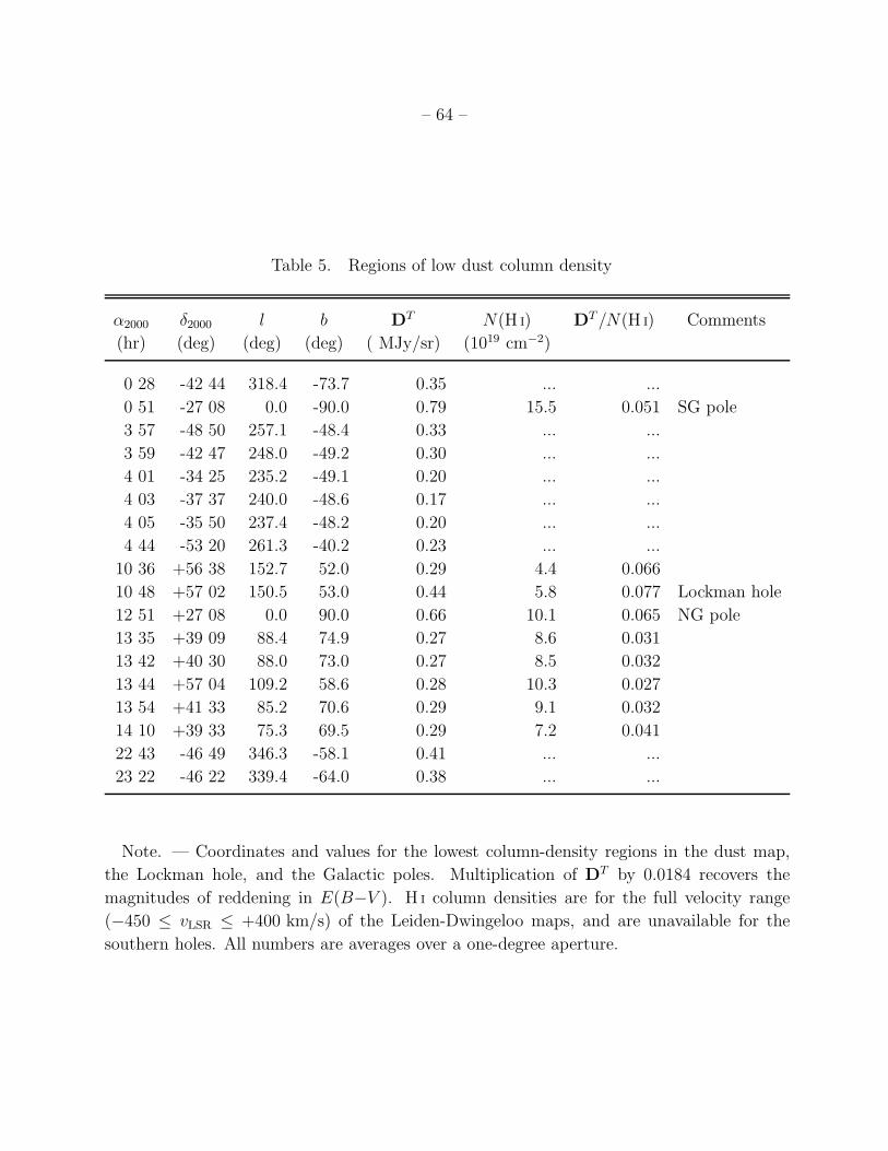
– 64 –

Table 5. Regions of low dust column density

α2000 δ2000 l b DT N(H I) DT /N(H I) Comments

(hr) (deg) (deg) (deg) ( MJy/sr) (1019 cm−2)

0 28 -42 44 318.4 -73.7 0.35 ... ...

0 51 -27 08 0.0 -90.0 0.79 15.5 0.051 SG pole

3 57 -48 50 257.1 -48.4 0.33 ... ...

3 59 -42 47 248.0 -49.2 0.30 ... ...

4 01 -34 25 235.2 -49.1 0.20 ... ...

4 03 -37 37 240.0 -48.6 0.17 ... ...

4 05 -35 50 237.4 -48.2 0.20 ... ...

4 44 -53 20 261.3 -40.2 0.23 ... ...

10 36 +56 38 152.7 52.0 0.29 4.4 0.066

10 48 +57 02 150.5 53.0 0.44 5.8 0.077 Lockman hole

12 51 +27 08 0.0 90.0 0.66 10.1 0.065 NG pole

13 35 +39 09 88.4 74.9 0.27 8.6 0.031

13 42 +40 30 88.0 73.0 0.27 8.5 0.032

13 44 +57 04 109.2 58.6 0.28 10.3 0.027

13 54 +41 33 85.2 70.6 0.29 9.1 0.032

14 10 +39 33 75.3 69.5 0.29 7.2 0.041

22 43 -46 49 346.3 -58.1 0.41 ... ...

23 22 -46 22 339.4 -64.0 0.38 ... ...

Note. — Coordinates and values for the lowest column-density regions in the dust map,

the Lockman hole, and the Galactic poles. Multiplication of DT by 0.0184 recovers the

magnitudes of reddening in E(B−V ). H I column densities are for the full velocity range

(−450 ≤ vLSR ≤ +400 km/s) of the Leiden-Dwingeloo maps, and are unavailable for the

southern holes. All numbers are averages over a one-degree aperture.

– 65 –

Table 6. Relative extinction for selected bandpasses

Filter λeff A/A(V ) A/E(B−V ) Filter λeff A/A(V ) A/E(B−V )

( A) ( A)

Landolt U 3372 1.664 5.434 Stromgren u 3502 1.602 5.231

Landolt B 4404 1.321 4.315 Stromgren b 4676 1.240 4.049

Landolt V 5428 1.015 3.315 Stromgren v 4127 1.394 4.552

Landolt R 6509 0.819 2.673 Stromgren β 4861 1.182 3.858

Landolt I 8090 0.594 1.940 Stromgren y 5479 1.004 3.277

CTIO U 3683 1.521 4.968 Sloan u′ 3546 1.579 5.155

CTIO B 4393 1.324 4.325 Sloan g′ 4925 1.161 3.793

CTIO V 5519 0.992 3.240 Sloan r′ 6335 0.843 2.751

CTIO R 6602 0.807 2.634 Sloan i′ 7799 0.639 2.086

CTIO I 8046 0.601 1.962 Sloan z′ 9294 0.453 1.479

UKIRT J 12660 0.276 0.902 WFPC2 F300W 3047 1.791 5.849

UKIRT H 16732 0.176 0.576 WFPC2 F450W 4711 1.229 4.015

UKIRT K 22152 0.112 0.367 WFPC2 F555W 5498 0.996 3.252

UKIRT L′ 38079 0.047 0.153 WFPC2 F606W 6042 0.885 2.889

Gunn g 5244 1.065 3.476 WFPC2 F702W 7068 0.746 2.435

Gunn r 6707 0.793 2.590 WFPC2 F814W 8066 0.597 1.948

Gunn i 7985 0.610 1.991 DSS-II g 4814 1.197 3.907

Gunn z 9055 0.472 1.540 DSS-II r 6571 0.811 2.649

Spinrad RS 6993 0.755 2.467 DSS-II i 8183 0.580 1.893

APM bJ 4690 1.236 4.035

Note. — The above tabulates the magnitudes of extinction evaluated in different passbands using the

RV = 3.1 extinction laws of Cardelli et al. (1989) and O’Donnell (1994). The final column normalizes the

extinction to photo-electric measurements of E(B−V ).