marital age homogamy in china: a reversal of trend … age homogamy in china: a reversal of trend in...
TRANSCRIPT


Marital Age Homogamy in China: A Reversal of Trend in the Reform Era?
ZHENG MU
University of Michigan
YU XIE
University of Michigan
_____________
Acknowledgments: An early version of this paper was presented at the 2009 International Sociological Association Research Committee 28 on Social Stratification and Mobility spring meeting in Beijing, China and the 2010 Population Association of America annual meeting in Dallas, Texas. We are grateful to Tak Wing Chan, Albert Esteve, Cindy Glovinsky, Alexandra Killewald, Qing Lai, Katherine Lin, Lin Ma, James Raymo, Christine Schwartz, Pam Smock, Arland Thornton, Berna Torr, Xiwei Wu, Jia Yu, Zhuoni Zhang, members of Quantitative Methodology Program at the University of Michigan and conference participants for their help and advice.
Corresponding Author: Direct all correspondence to Zheng Mu, Room 2067, 426 Thompson Street, Population Studies Center, Institute for Social Research, University of Michigan, Ann Arbor, MI 48106-1248. Phone: 734-358-8715. Email: [email protected].

Marital Age Homogamy in China 2
INTRODUCTION
Social homogamy refers to the degree to which individuals with similar social
characteristics marry each other (Burgess and Wallin 1943). Practiced in a variety of societies,
social homogamy has captured the attention of researchers interested in marriage and social
stratification. In this literature, an increase in homogamy based on such attributes as
socioeconomic status, education, and race and ethnicity has been considered indicative of a
decline in social openness and an increase in social inequality (Mare 1991; Kalmijn 1991, 1998;
Smits, Ultee, and Lammers 1998; Raymo and Xie 2000; Harris and Ono 2005; Schwartz and
Mare 2005; Mare and Schwartz 2006; Schwartz 2010; Torche 2010; Zijdeman and Maas 2010).
Compared to other forms of social homogamy, age homogamy has received less attention
among researchers. Age homogamy, however, is also an important indicator of social closure and
gender inequality, as large age differences between spouses have been associated with more
patriarchal family systems and less spousal intimacy (Van Poppel et al. 2001; Blossfeld 2009;
Van de Putte et al. 2009). While the literature contains several studies on age homogamy (e.g.,
Atkinson and Glass 1985; Van Poppel et al. 2001; Esteve, Cortina, and Cabré 2009; Van de Putte
et al. 2009), none deals with a long-term trend in contemporary China, particularly reform-era
China.
Our study covers trends in age homogamy in China between 1960 and 2005, using
indicators based on Schoen’s forces of attraction (Schoen 1981, 1988; Qian and Preston 1993;
Esteve et al. 2009). We use a random sample of the nationally representative China 2005 1%
Population Inter-census Survey (also called 2005 mini-census). Instead of a consistent increase,
as expected from the existing literature, results surprisingly show an inverted U-shaped trend in

Marital Age Homogamy in China 3
age homogamy. One plausible explanation is the reversal towards “necessity considerations” in
mate-selection during the post-1990 reform era.
RESEARCH BACKGROUND
Age Homogamy and Modernization
A large literature in sociology has explored trends in social homogamy (Atkinson and
Glass 1985; Mare 1991; Kalmijn 1991, 1993, 1998; Qian 1997; Raymo and Xie 2000; Van
Poppel et al. 2001; Schwartz and Mare 2005; Qian and Lichter 2007; Esteve et al. 2009; Song
2009; Van de Putte et al. 2009; Han 2010; Zijdeman and Maas 2010). In this literature, social
homogamy is widely considered a measure of social closure or cleavage (Smits et al. 1998;
Raymo and Xie 2000; Van Poppel et al. 2001; Schwartz and Mare 2005; Zijdeman and Maas
2010), which is generally expected to lessen during periods of economic development
accompanied by more egalitarian and liberal social values (Goode 1970; Kalmijn 1991, 1993,
1998; Qian 1997; Raymo and Xie 2000; Qian and Lichter 2007).
Age homogamy, however, should be conceptualized as a unique form of social
homogamy and, as such, differs radically from other forms of social homogamy in its theoretical
implications. Whereas homogamy in other social attributes reveals inequality and social closure,
age homogamy between spouses is indicative of gender equality and social openness (Casterline,
Williams, and McDonalds 1986; Wheeler and Gunter 1987; Van Poppel et al. 2001). From a few
studies of trends in age homogamy, the consensus so far is that economic development is
associated with either an increase in age homogamy or no clear trend (Atkinson and Glass 1985;
Qian 1998; Van Poppel et al. 2001; Esteve et al. 2009; Van de Putte et al. 2009; Casterline, Qian,
and Liu 2010).
Marital Age Homogamy in China 4
To see why this is the case, let us first consider the traditional family patterns in most
societies before industrialization. While we acknowledge variations in practice at both the
societal and the individual levels, the traditional family is characterized by a relatively large age
gap between an older, bread earner husband and his younger wife (Van Poppel et al. 2001). This
pattern supports the patriarchal family system by reinforcing the husband’s authority and
impeding spousal intimacy (Cain 1993; Van Poppel et al. 2001; Barbieri, Hertrich, and Grieve
2005). However, with industrialization and women’s increasing economic roles outside the home
in modern societies, the average age gap between the husband and the wife narrows. In this
context, a trend towards smaller age gaps, i.e., age homogamy, is taken to indicate a change
towards gender equality and love-based (as opposed to necessity-based) marriages (Bozon 1991;
Van Poppel et al. 2001; Van de Putte et al. 2009).
To better understand why spousal age gap may be affected by modernization, we now
turn to Kalmijn’s (1991, 1998) general framework for explaining social homogamy. Within his
framework, three sets of factors need to be considered: (1) the preferences of marriage
candidates, (2) the impact of a “third party” (marriage candidates’ parents, for example), and (3)
the interaction structures of the marriage market. All the factors are affected, in favor of age
homogamy, by the process of economic development (Smits et al. 1998; Raymo and Iwasawa
2005; Song 2009).
By preference, social researchers commonly mean individuals’ choices free of structural
constraints and motivated by their own social values and beliefs. Marriage is a social institution
that binds two persons together in an intimate living relationship. Of course, people may get
married for different reasons: some for economic exchange, some for family or even national
interests, and some for romantic love. As a society changes from an agricultural society to a

Marital Age Homogamy in China 5
modern, industrial one, however, romance becomes increasingly the accepted and even the
predominant basis for marriage (Xu and Whyte 1990; Thornton and Lin 1994). Admittedly,
persons of different ages can and do form strong bonds based on romantic love, but romance is
most likely to develop when partners interact directly and share similarities in such
characteristics as age, culture, tastes and physical conditions (Bhrolchain 1992; Van Poppel et al.
2001). Consequently, a shift to a love-based mate-selection norm is more likely to lead to smaller
age differences (Wheeler and Gunter 1987; Bozon 1991; Van Poppel et al. 2001).
Moreover, it is well established that as a society is transformed from an agriculture-based
to an industry-based economy, individuals themselves rather than parents or other authority
figures increasingly make decisions about family-related behaviors (Goode 1970; Xu and Whyte
1990; Thornton and Lin 1994; Thornton 2001; Barbieri et al. 2005; Thornton, Axinn and Xie
2007). That is, one clear implication of development is the diminished impact of the “third party”
and the freedom of young individuals to choose their own mates. When youth are left on their
own to choose their potential spouses, their choices may be limited to those whom they know
best – most likely peers of similar ages to their own – and thus reduce the spousal age difference
(Casterline et al. 1986; Wheeler and Gunter 1987; Bozon 1991; Van Poppel et al. 2001).
Besides preference and the impact of the “third party,” the structure of the marriage
market can also be affected by economic development (Bytheway 1981; Atkinson and Glass
1985; Vera, Berardo, and Berardo 1985; Kalmijn 1991, 1998; Bhrolchain 1992; Stier and Shavit
1994; Lichter, Anderson, and Hayward 1995; Todd, Billari, and Simão 2005). For example, with
industrialization, educational attainment generally increases. As a result, youth spend an
increasingly large fraction of their pre-marital years in school, resulting in a much higher
probability of finding a spouse among schoolmates before completing their education. This may

Marital Age Homogamy in China 6
be especially true for those receiving higher education, as the timing for pursuing postsecondary
education is highly similar to that for selecting marriage partners. Therefore, lengthened
education completion may transform postsecondary institutions into important marriage markets
and thus may increase the incidence of age homogamy between schoolmates (Mare 1991;
Blossfeld and Timm 2003).
For these reasons, a consensus emerges in the existing literature that economic
development should generally lead to a rise in age homogamy. This prevailing theoretical view is
also supported by empirical evidence from a variety of countries. For example, a recent study by
Casterline et al. (2010) reports that out of the twenty-four developing countries under study,
seventeen experienced an increase in percentages of couples with age gaps (husband’s minus
wife’s) between 0-5 years (zero and five included). The increases ranged from as low as 0.2% for
Peru between 1977 and 2004 to as high as 20.5% for Ghana between 1979 and 2008. Developed
countries experienced similar increases. The percentage of couples with age gaps within four
years (four included) for the United States increased from 37.1% in 1900 to 63.3% in 1960 and
69.9% in 1980 (Atkinson and Glass 1985). The percentage of marriages with age gaps less than
two years (two excluded) rose by 7%-20% for the Dutch regions between 1812 and 1913 (Van
de Putte et al. 2009). The proportion of spouses within the same five-year age categories (five
included) increased from 35% in the mid-nineteenth century to more than 50% in the 1970s and
early 1980s for the Netherlands (Van Poppel et al. 2001). The same percentage for Spain
increased from 36% in 1944 to 49% in 2000 (Esteve et al. 2009). Thus, previous studies all
indicate a secular decline in the age gap between spouses, particularly during periods of
development. Is this generalization universal? Specifically, does it hold true for China in its
recent past?
Marital Age Homogamy in China 7
The Chinese Context
The People’s Republic of China was founded in 1949 after the Communist Revolution.
For the first 30 years, China suffered from numerous political conflicts, and the Communist
ideology for equality prevailed (Meisner 1999; Whyte 2010). In 1978, China began its economic
reform, leading to dramatic improvements in economic and educational outcomes (Xie and
Hannum 1996; Qian 2000; Wu and Xie 2003; Hauser and Xie 2005; Whyte 2010). For example,
from 1978 to 2005, China’s per capita GDP grew from 381 yuan to 2,062 inflation-adjusted
yuan, averaging an annual growth rate of 6.45% (China Statistics Press 2006: Table 3-1, 3-17).
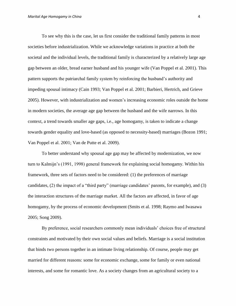
In terms of education, from 1978 to 2005, the proportion of population enrolled in postsecondary
institutions grew from 0.09% to 1.19% (China Statistics Press 2006: Table 4-1, 21-6),1 while
from 1982 to 2005, the illiteracy rate dropped tremendously from 31.87% to 11.04%2 (China
Statistics Press 1985: Table 6 of the Third Census Document; 2006: Table 4-13). For persons
aged 25-29, the age range in which marriage usually occurs, the percentage completing
postsecondary education grew dramatically from 1.04% in 1982 to 12.66% in 2005 (China Data
Center 1982: Table 5-48; 2005: Table 4-1).
Throughout the history of modern China since 1949, women’s social standing has been
improving. In 1950, China instituted the Marriage Law, which formally legalized free-choice
marriages and explicitly protected wives’ rights and interests, equal to those of husbands (China
Administration Council 1950: Item 5). Women’s socioeconomic status has also significantly
1 All percentages completing postsecondary education in this sentence and in the next paragraph were
computed as ratio of population completing postsecondary education over that receiving any education,
due to data availability.
2 The base for the 1982 illiteracy rate is population 12 years and older, and that for the 2005 illiteracy rate
is population 15 years and older. This comparison gives us a conservative evaluation of the drop in
illiteracy.

Marital Age Homogamy in China 8
improved (Lavely et al. 1990; Hannum and Xie 1994; Hannum 2005; Zhang, Hannum, and
Wang 2008; Song 2009). In education, women’s attainment has gradually caught up with that of
men (Hannum and Xie 1994; Wu and Song 2010: Table 2; Wu and Zhang 2010). For instance, in
1982, the percentages receiving postsecondary education were respectively 1.24% for men and
0.64% for women; these percentages increased to 6.72% and 5.63% in 2005, narrowing men’s
advantage from about 100% to only about 20% (China Data Center 1982: Table 5-46; 2005:
Table 4-1).
This change in women’s social status has challenged status hypergamy – the tendency of
women to marry men of higher social status – a traditional practice for marriages in China and
other East Asian countries (Yang 1959; Freedman 1970; Meijer 1971; Baker 1979; Croll 1981;
Watson and Ebrey 1991; Xu, Ji, and Tung 2000; Fan and Li 2002; Raymo 2003; Raymo and
Iwasawa 2005; Dasgupta, Ebenstein and Sharygin 2010). Chinese society traditionally
maintained a patriarchal and patrilineal family system (Thornton and Lin 1994; Xu et al. 2000;
Xie and Zhu 2009). Due to the restricted access of women to work outside households, their
social statuses were determined by the social standings of their parents before marriage and their
husbands after marriage. Under this rigid patriarchal system, men customarily assumed the role
of primary bread earners with higher socioeconomic statuses than their wives. Thus, status
hypergamy was prevalent in traditional Chinese society as a cultural norm. With women’s
improvement in socioeconomic status, particularly in education, it becomes increasingly harder
to maintain status hypergamy.
These social changes in modern China – increasing free choice in mate selection,
improvement in economic well-being, and rise of women’s social status – provide the
appropriate context in which we can interpret trends in age homagamy in China since 1960.

Marital Age Homogamy in China 9
According to the existing literature we reviewed in the preceding subsection, these changes
should all have been in favor of increasing age homogamy for contemporary China. Has the
actual trend been a steady increase in age homogamy? This is an empirical question that we
address in this paper.
DATA AND METHODS
This study uses both descriptive statistics and homogamy indicators based on “forces of
attraction” (Qian and Preston 1993; Esteve et al. 2009). In order to examine the robustness of the
descriptive results, we also apply log-multiplicative layer effect models using year of marriage as
the layer variable. Due to space limitation, we do not report all the results. The data are based on
a random sample of the China 2005 1% Population Inter-census Survey (also called 2005 mini-
census).
Analytical Samples
We first restrict our analysis to individuals aged 15 and older in order to exclude those ineligible
for marriage. Next, to compute forces of attraction, we construct, for each year being studied,
two subsamples: one of single individuals, and the other of couples. Because we need to
construct these subsamples retrospectively from data in 2005, we are concerned with the effect
of mortality, given women’s lower mortality than men’s (Yaukey, Anderton, and Lundquist
2007), which may result in severe underestimation of spousal age gaps for earlier cohorts. Hence,
we restrict both “single” and “couple” subsamples to marriage cohorts between 1960 and 2005.
For the “single” subsample, we set the marriageable age range at 15 to 50 for each
marriage cohort. Note that, we need to construct a pool of single persons at risk of marrying for
each marriage cohort, including those who were married later. Therefore, this reconstructed
subsample of “singles” includes all persons aged between 15 and 95 in 2005, and married
Marital Age Homogamy in China 10
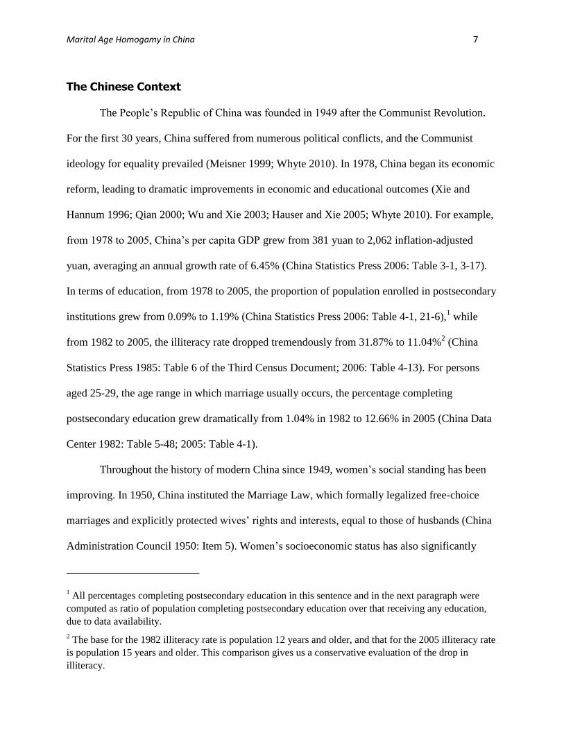
between 1960 and 2005 or still single in 2005. These restrictions leave us with a total of
1,880,015 individuals, with 947,324 males and 932,691 females respectively.
For the “couples” subsample, we restrict the data to those couples in which both partners
were married for the first time that year, forming the marriage cohort. These restrictions result in
a total of 459,721 couples for marriage cohorts between 1960 and 2005. We use this larger
“couple” sample for descriptive analyses and log-multiplicative layer effect models. However, to
compute homogamy indicators based on forces of attraction, we further restrict the sample to
couples with both partners’ ages at first marriage between 15 and 50 corresponding to the
assumed marriageable age range. This additional restriction reduced only a small number of
cases, resulting in a total of 459,291 couples.
Past studies on trends in homogamy have relied on repeated cross-sectional data of
recently contracted marriages or newlyweds, to avoid bias from selective marital dissolution or
remarriage (e.g., Mare 1991; Qian and Preston 1993; Kalmijn 1994; Qian 1998; Raymo and Xie
2000; Schwartz and Mare 2005). Note that information about age at marriage is available only on
the 2005 mini-census but on not regular censuses. We capitalize on this unique feature of the
2005 mini-census data and reconstruct, retrospectively, the experiences of marriage cohorts from
this later cross-sectional dataset. Due to data limitation, we restrict our analysis to first marriages,
and as based on the abovementioned literature, this may introduce a bias to our study. Given the
very low divorce rates in China throughout this period, however, we do not see this as a severe
problem.3 Still, it is useful to speculate on the direction of such biases. As many scholars of
marriage have argued, larger spousal age differences often predict higher risks of divorce (Day
3 Divorce rates range from as low as 0.035% in 1980 to as high as 0.137% in 2005 (China Statistics Press,
2006).

Marital Age Homogamy in China 11
1964; Bumpass and Sweet 1972; Levinger 1976; Wilson and Smallwood 2008), and additionally,
higher marriage parity usually relates to larger spousal age gaps (Dean and Gurak 1978;
Atkinson and Glass 1985; Vera et al. 1985; Bhrolchain 1992). Given the rise in divorce rates, our
focus on the prevailing first marriages is likely to exert a bias towards a heightened trend in age
homogamy, increasingly so for more recent periods.
Additionally, due to the cross-sectional nature of the 2005 mini-census dataset, a majority
of the younger individuals in 2005 may have not yet completed their mate selection process.
Thus, our sample may include a disproportionately higher proportion of younger marriages for
this age group. According to the literature, later marriages usually relate to larger age gaps (Qian
1998; Van Poppel et al. 2001). Hence, there should be an overestimation for the level of age
homogamy for later marriage cohorts due to higher percentage of younger age groups in those
cohorts.
Homogamy Indicators
The concept of force of attraction was first introduced by Schoen (1981, 1988). It is a
special type of marriage rate based on the harmonic mean of single males and females, i.e., those
at risk of marriage, for each spousal age combination. The mathematical formula of force of
attraction is:
( ) ( )
ij
iji j
i j
m
H W
H n W n
, (1)
in which ijm indicates the number of marriages between males aged i and females aged j ;
iH and jW respectively identifies the number of eligible males at age i and that of eligible
females at age j ; n is length of the age intervals. In this formula, the number of marriages that

Marital Age Homogamy in China 12
are actually contracted is considered along with the amount of potential exposure between
eligible males aged i and females aged j . Thus, the population at risk of marriage is taken into
account. Compared to investigation only considering prevailing marriages, our analysis controls
for changes in age-sex composition of the marriage market.
For each marriage cohort, we calculate a homogamy indicator based on forces of
attraction (Esteve et al. 2009). The homogamy indicator is the ratio of sum of forces of attraction
( ij as defined in Equation (1)) where i equals j , over the sum of all forces of attraction. This
indicator reflects the strength of preferences for age homogamy over the overall distribution of
couples. It ranges from 0 to 1 – the larger the indicator, the stronger the preference for age
homogamy.
We construct forces of attraction and homogamy indicators respectively with single-year,
three-year and five-year age groups. As Van Poppel and colleagues (2001) demonstrated,
dividing age at marriage into groups with mandatorily determined boundaries and widths can
only identify level of heterogamy with relatively large spousal age gaps and thus may produce
inaccurate results. Furthermore, this approach may classify some marriages with a small age gap
(eg., with husband marrying at 35 and wife at 34) as heterogamy, while classifying others with a
large age gap (with husband marrying at 34 and wife at 30) as homogamy. Therefore,
experimenting with changing age groupings enables us to mitigate the negative impact of
categorization by observing robustness of the results. These different groupings can also provide
levels of age homogamy based on definitions of varying strictness. While homogamy indicators
with single-year age groups define age homogamy in the most conservative sense, those with
five-year age groups provide much more liberal definitions.

Marital Age Homogamy in China 13
RESULTS
Trend in Marital Age Homogamy
Figure 1 presents results on trends in age homogamy using different descriptive measures
of spousal age gaps. The bottom line shows proportions of couples with no age gap – the most
conservative definition of age homogamy. The line right above it shows proportions of couples
with an age gap of [0, 1], and then [0, 3]. The top line shows the most liberal definition of age
homogamy with the broadest age gap of [-1, 4]. As can be seen from the figure, the four lines
provide very similar trends. However, to our surprise, rather than a consistent increase, all four
lines demonstrate increases from the start of the series to the early 1990s and salient decreases
thereafter.
0
20
40
60
80
Pe
rcen
tage
1960 1965 1970 1975 1980 1985 1990 1995 2000 2005
Marriage Cohort
Husband-Wife Age Gap=0 [0,1]
[0,3] [-1,4]
Note: Percentages are calculated by dividing number of couples with the given age gapby the total number of couples of the marriage cohort.Source: National Bureau of Statistics of China, China 2005 1% Population Inter-census Survey.
Figure 1 Percentage of Different Levels of Age Homogamy1960-2005
We obtain a similar inverted U-shaped trend using homogamy indicators by forces of
attraction, with all three age groupings. As can be seen in Figure 2, level of age homogamy rose

Marital Age Homogamy in China 14
continuously after 1960 but dropped from the early 1990s on. This analysis is not a repetition of
those shown in Figure 1. By using homogamy indicators, we can evaluate underlying preferences
of age homogamy while controlling for the confounding influence of the age-sex composition of
the marriage market.
0
.1
.2
.3
.4
.5
.6
Hom
oga
my Ind
ica
tor
1960 1965 1970 1975 1980 1985 1990 1995 2000 2005
Marriage Cohort
single year three years
five years
Note: Homogamy indicators are constructed as the ratio of sum of forces of attraction (as definedin Equation(1)) where equals, over the sum of all forces of attraction for marriage cohort 1960-2005,respectively with age in single-, three- and five-year groups. Larger indicators reflect higherlevels of marital age homogamy.Source: National Bureau of Statistics of China, China 2005 1% Population Inter-census Survey.
Figure 2 Levels of Age Homogamy by Force of Attraction1960-2005
Both sets of trends shown in Figures 1 and 2 deviate from our expectations. The earlier
trends, up to the early 1990s, confirm our expectation, since social development should have led
to more love-based marriages and smaller spousal age gaps, as predicted by the established
positive relationship between age homogamy and social development (Van Poppel et al. 2001).
However, since the early 1990s, the trend started to reverse, leading to an inverted U-shape for
the entire period under study.

Marital Age Homogamy in China 15
Is the reversal real? In order to observe the trends more clearly, we computed moving
averages for the three sets of homogamy indicators, with equal and varying weights for the
adjacent three, five, seven, nine and eleven marriage cohorts respectively. Appendix Tables A1
to A3 contain computed homogamy indicators based on the three sets of age groupings. As can
be seen from these results, the inverted U-shaped trend in age homogamy holds true for all
different age groups and for varying methods of computing moving averages. Among them, the
trend based on three-year age groups is especially sharp. Therefore, we present in Figure 3 the
trends based on three-year age groups respectively with raw homogamy indicators and their
moving averages for the adjacent seven marriage cohorts with equal weights.
.18
.2
.22
.24
.26
.28
Hom
oga
my Ind
ica
tor
1960 1965 1970 1975 1980 1985 1990 1995 2000 2005
Marriage Cohort
moving average raw
Note: Raw homogamy indicators are constructed as the ratio of sum of forces of attraction(as defined in Equation(1)) where equals, over the sum of all forces of attraction for marriage cohort1960-2005, with age in three-year groups. Their moving averages are constructed by averagingthe raw homogamy indicators for the adjacent seven marriage cohorts with equal weights.Larger indicators reflect higher levels of marital age homogamy.Source: National Bureau of Statistics of China, China 2005 1% Population Inter-census Survey.
Figure 3 Levels of Age Homogamy by Force of Attractionwith Moving Average 1960-2005
As can be seen, the two trends based on raw indicators and their moving averages are
generally consistent with each other in spite of short-term fluctuations shown in the raw
indicators. The trend based on moving averages is clear: From 1960 to the mid-1960s, there was

Marital Age Homogamy in China 16
a slight increase in level of age homogamy, and the trend was unstable around the period of
Cultural Revolution between 1967 and 1976. Starting from the mid- to late-1970s, there was a
sharp increase until the early 1990s, when a drop began. We also conduct analysis based on log-
multiplicative layer effect models (Xie 1992; Raymo and Xie 2000) with varying design
matrices, and an inverted U-shaped trend keeps showing for all the models used.4
As discussed earlier, all of our sample construction and restriction methods should lead to
overestimation of levels of age homogamy for later marriage cohorts. Regarding this, we
consider the observed reversal of the trend in age homogamy, from more homogamy to less
homgamy after the early 1990s, conservative. The actual reversal without the data limitations
should even be more pronounced than that revealed by our data.
Separation of Hypogamy and Hypergamy
As shown above, a consistent increase in levels of age homogamy along the course of
development was disrupted during the post-1990 reform era. A decline in age homogamy in the
more recent period suggests that either hypogamy (i.e., an older wife marrying a younger
husband) or hypergamy (i.e., a younger wife marrying an older husband), or both, has increased.
However, theoretical implications of these two alternatives are quite different. For example,
while an increase in age hypogamy may indicate more liberal attitudes on gender relations and
marriage, a rise in age hypergamy may reflect quite the opposite, with the husband resuming
their power over the wife. Therefore, distinguishing changes in either age hypogamy or
hypergamy could shed light on the potential explanations for the reversal trend in age
homogamy.
4 These results are posted on the author’s website.
Marital Age Homogamy in China 17
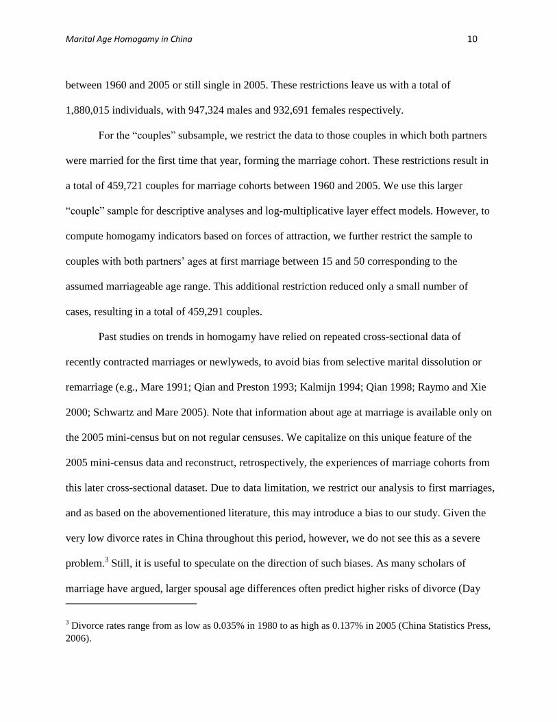
As can be seen in Figure 4, the trend in age hypogamy increased from 1960 all the way
towards early 1990s and decreased afterwards. While we may attribute the increase to more
liberal attitudes on age differences in the earlier period, the decrease in the more recent period is
puzzling. However, for our purpose of explaining the recent decrease in age homogamy, this tells
us that more older women marrying younger husbands is not likely to be the reason for the
decline in age homogamy in the more recent period.
0
5
10
15
20
Pe
rcen
tage
of A
ge
Hypo
ga
my
1960 1965 1970 1975 1980 1985 1990 1995 2000 2005
Marriage Cohort
Note: As shown are percentages of age hypogamy for each marraige cohort of 1960-2005.Source: National Bureau of Statistics of China, China 2005 1% Population Inter-census Survey.
Figure 4 Percentage of Marital Age Hypogamy, 1960-2005
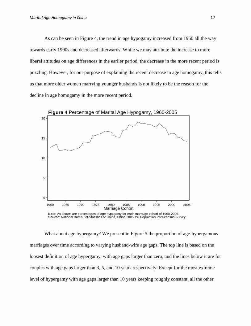
What about age hypergamy? We present in Figure 5 the proportion of age-hypergamous
marriages over time according to varying husband-wife age gaps. The top line is based on the
loosest definition of age hypergamy, with age gaps larger than zero, and the lines below it are for
couples with age gaps larger than 3, 5, and 10 years respectively. Except for the most extreme
level of hypergamy with age gaps larger than 10 years keeping roughly constant, all the other

Marital Age Homogamy in China 18
lines present similar trends, with percentages of age hypergamy decreasing from 1960 to the late
1980s, then increasing from the early 1990s on.
0
20
40
60
80
Pe
rcen
tage
1960 1965 1970 1975 1980 1985 1990 1995 2000 2005
Marriage Cohort
Husband-Wife Age Gap>0 3+
5+ 10+
Note: Percentages are calculated by dividing number of couples with the given age gapby the total number of couples of the marriage cohort.Source: National Bureau of Statistics of China, China 2005 1% Population Inter-census Survey.
Figure 5 Percentage of Different Levels of Age Hypergamy1960-2005
The pattern shown by Figure 5 echoes those pertaining to age homogamy in Figures 1 to
3. That is, during the most recent post-reform era since the early 1990s, more individuals have
retreated from age homogamy and chosen age hypergamy instead. Why hypergamy? What is so
special about the post-1990 reform era? In the next section we will discuss a possible explanation
for the reversal in age homogamy.
Economic Pressure: An Explanation for the Reversal
At first glance, the decrease in marital age homogamy and the corresponding increase in
age hypergamy since the early 1990s are surprising in terms of the widely believed positive
relationship between age homogamy and development. However, as mentioned earlier, status
hypergamy was widely practiced in traditional China (Thornton and Lin 1994; Xie and Zhu

Marital Age Homogamy in China 19
2009). Thus, while age hypergamy was substantially eroded after the founding of the People’s
Republic of China in 1949, there may be reasons for it to return in the post-1990 reform period.
In contrast with other periods examined in this paper, the reform era has been one not
only of rapid economic growth and a sharp increase in standard of living, but also of a
tremendous rise in consumer aspirations accompanied by increasingly severe market competition.
Those social forces may have influenced marital decisions in different or even opposite ways.
First, from the bride’s standpoint, increasingly severe competition within the labor
market during the post-1990 reform era may have brought women back to a disadvantaged
position. Some researchers (Summerfield 1994; Zhang et al. 2008) have found that a narrow
emphasis on short-term efficiency and profit-making among many companies during more recent
reform-era has led to greater discrimination against women within the labor market. In recent
years, women’s unemployment increased significantly (Summerfield 1994; Wu and Song 2010:
Table 2). Facing this new, unfavorable labor market environment, many women may be
involuntarily forced back into traditional homemaker roles. In light of their “downgraded” role in
the labor market, marrying a “good” husband with respect to his socioeconomic conditions has
once again become an attractive channel to higher social status. Since older men are more likely
to possess higher social status and greater economic potential, this may make older husbands
more appealing (Bozon 1991).
Second, from the groom’s standpoint, men now also face increasingly fierce market
competition and higher costs of establishing households. Women’s resumption of housewife
roles and retreat to the necessity considerations may be associated with men’s increasing
problems in matters of career and marriage. Just as women are forced back into the role of
homemakers, men are now more likely to be stuck in the role of bread earners. Considering the

Marital Age Homogamy in China 20
conventional practice of status hypergamy, men also face greater pressures to accumulate richer
socioeconomic resources given women’s enhanced educational profiles (Raymo and Iwasawa
2005). Thus, they have to compete in both the labor and the marriage markets, with competition
ever more intense on both fronts. To become more attractive to women during this double
contest, men need to wait longer while accumulating resources (Thornton, Axinn and Teachman
1995; Smock and Manning 1997; Xie et al. 2003).
Therefore, while women may begin to marry older men in response to their occupational
downgrades, men may need to settle down later by virtue of the double competitions they face.
These tendencies, generated by the economic reforms, may eventually have led to larger age gaps
between husbands and wives in the later stage of the reform. That is, the positive influence of
economic growth on age homogamy may have been counteracted by an opposing social force
resulting from increased market competition. The same process of the reform that helped narrow
spousal age gaps in the early years may, since the early 1990s, have contributed to the widening
of spousal age gaps due to intensified competition. For convenience, we call this the “economic
pressure” explanation.
Theoretically speaking, status hypergamy can be attained through a variety of channels.
Women can marry up in terms of achieved traits such as education and occupation, or ascribed
traits such as family origins and race/ethnicity. Among these domains, age and education are
especially important. Age is tightly related to overall socioeconomic status, since older
individuals are more likely to accumulate greater cultural and social resources (Van Poppel et al.
2001). Moreover, a normative large spousal age gap with the husband older than the wife is
believed to efficiently facilitate the traditional division of labor within the household (Wheeler
and Gunter 1987; Van Poppel et al. 2001). Thus, women may marry older husbands with

Marital Age Homogamy in China 21
established status so as to achieve status hypergamy (Bozon 1991). At the same time, education
has been well established as a predictor of socioeconomic conditions (Mincer 1974; Mare 1991;
Xie and Hannum 1996; Xu et al. 2000; Wu and Xie 2003; Hauser and Xie 2005; Schwartz and
Mare 2005) as well as a reflection of one’s family origins (Mare 1991; Raftery and Hout 1993;
Lucas 2001; Blossfeld and Timm 2003). Hence, women often choose to marry husbands with
more education than they have received themselves so as to realize status hypergamy.
Note that women’s educational attainment has increased dramatically during China’s
post-1949 history (Lavely et al. 1990), resulting in a rapid narrowing of the gender gap in
education (Hannum and Xie 1994; Hannum 2005). This trend may be a unique contributing
factor in reversing the trend towards age homogamy. While the economic pressure for status
hypergamy intensified during the post-1990 reform era, it also became increasingly difficult for
highly educated women to find husbands with enough education to satisfy the expectation of
education-based hypergamy. In Figure 6, for example, we observe that, since the late 1970s and
especially since the early 1990s, males’ and females’ educational levels have gradually
converged. Specifically, the ratio of spousal educational gap (husband’s minus wife’s) to wives’
years of schooling has decreased from as high as 0.27 in 1960 all the way down towards 0.03 in
2005. The narrowing gender gap in education has made it ever more difficult to practice
hypergamy with respect to education. Thus, couples may elect to achieve hypergamy instead by
means of age, widening the age gap so that the husband still maintains an economic advantage
over his similarly educated but less experienced wife. Therefore, during the post-1990 reform
era, the notion of “marrying up” may have reemerged with a different meaning: the husband
tending to be older and economically better off than the wife, though not necessarily better
educated.

Marital Age Homogamy in China 22
0
2
4
6
8
10
Ye
ars
of S
ch
oo
ling
1960 1965 1970 1975 1980 1985 1990 1995 2000 2005
Marriage Cohort
Husband Wife
Note: As shown are the average years of schooling of husbands and wivesfor each marraige cohort of 1960-2005.Source: National Bureau of Statistics of China, China 2005 1% Population Inter-census Survey.
Figure 6 Husbands' and Wives' Average Years of Schooling1960-2005
To test this conjecture, we conduct an auxiliary analysis based on a revised version of
Mincer’s (1974) human capital model. In this analysis, we consider what possible role the
narrowing gender educational gap may have played as a concrete causal mechanism for the
economic pressure explanation. Because we do not have perfect data for this part, this analysis is
intended mainly to demonstrate the relevance of this causal mechanism. The key idea is that the
spousal age gap may serve to compensate for the decreased spousal educational gap so as to
maintain status hypergamy. That is, during the later stage of the economic reform, age may have
begun to substitute for education as an effective proxy for men’s richer socioeconomic resources,
in the face of emerging convergence in educational attainment by gender.5
5 We are also aware that as higher education becomes more prevalent, postsecondary institutions may
play an increasingly important role as locations for mate selection. Conducting the mate selection process
in schools may lead to both educational and age homogamy. Under this circumstance, if the level of age
Marital Age Homogamy in China 23
We compare husbands’ earnings premiums by holding average educational attainment
and average age at first marriage at different levels for each marriage cohort. Lacking historical
data on couples’ earnings at the time of marriage, we instead resort to an estimation of their
potential earnings through a revised version of Mincer’s (1974) human capital model, in which
the estimated earnings of the year of marriage are based on the average educational attainment
and years of work experience for each marriage cohort. Specifically, we use the following
equation for each sex:
0 1 1 2 2lnY X X , (2)
where Y is earnings, X1 years of schooling, and X2 years of work experience. All ’s are
unknown parameters, and is the residual unexplained by the model. Equation (2) deviates
from Mincer’s model in that it does not include the quadratic term of years of work experience.
This is reasonable given that we restrict the analysis to persons aged between 20 and 30, the age
range in which most marriages occur and work experience increases earnings steadily. Thus,
inclusion of the quadratic term is not theoretically compelling and may result in a loss of
precision and predictive power of the model.
We use data from Chinese Household Income Project (CHIP) 1988, 1995 and 2002 to
estimate ’s in Equation (2), respectively for marriage cohorts 1985-1991, 1992-1998 and 1999-
2005. We use data only for urban workers because personal earnings are ambiguous for rural
residents in CHIP. Again, because our main objective here is illustrative, a systematic bias in the
auxiliary analysis resulted from the restriction to urban workers should not invalidate the
substantive conclusion. Given our specific purpose to estimate husbands’ earnings premiums, as
homogamy still decreases in the post-1990 reform era, we can claim stronger evidence for the potential
return to necessity considerations in mate selection.

Marital Age Homogamy in China 24
well as the gender differential in returns to education and experience, we estimate Equation (2)
separately for men and women. Combined with other criteria for excluding observations with
missing or incomplete data, this procedure yields samples of 2,052 men and 2,321 women from
CHIP 1988, 1,013 men and 1,060 women from CHIP 1995 and 640 men and 709 women from
CHIP 2002. We capture all forms of income, including the provision of cash bonuses and
subsidies. Earnings in 1995 and 2002 are adjusted by the appropriate price indices so that all
analyses are comparable in 1988 Yuan (China Statistics Press 2006). Following Xie and Hannum
(1996), we recode education into years of schooling for education6 and calculate work
experience as the difference between current age and age at first year of experience, which varies
with education.7
Once we obtain estimated ’s, we apply average years of schooling and average age at
first marriage for each marriage cohort using 2005 mini-census data to the regression equations
so as to estimate earnings at the time of marriage. Here we extrapolated years of work experience
from years of schooling and age at first marriage. In the end, we are able to estimate husband’
earnings premiums to wives’ with
^
^ln( )Husband
Wife
Earnings
Earnings
by marriage cohort. To explicitly
illustrate the role of increase in the spousal age gap in compensating for decrease in the
educational gender gap, we construct four trends according to (1) whether education was fixed to
6 Less than three years of schooling=1; three years of schooling but less than primary school=4; primary
school=6; junior high=9; senior high=12; trade school=13; community/technical college=15; college and
graduate school=17.
7 Specifically, the ages at first year of experience for each educational level are: primary school and
lower=14; junior high=16; senior high=19; trade school=20; community/technical college=22; college
and graduate school=24.

Marital Age Homogamy in China 25
the 1985 level or was allowed to change as it actually did, and (2) whether age at first marriage
was fixed to the 1985 level or was allowed to change as it actually did. The combination of these
two specifications yields four trends of husbands’ earnings premiums to wives’, one observed
and three hypothetical: (a) that based on observed average educational attainment and average
age at first marriage; (b) that based on observed average educational attainment, with average
age at first marriage held at the level of 1985; (c) that based on observed average age at first
marriage, with average educational attainment held at the level of 1985; and (d) that with both
average educational attainment and age at first marriage held at the level of 1985. The results are
shown in Figure 7.
0
.05
.1
.15
.2
.25
.3
.35
.4
ln(h
usb
an
ds' ea
rnin
gs/w
ive
s'e
arn
ing
s)
1985 1990 1995 2000 2005
Marriage Cohort
(a).Observed Education and Age at First Marriage (b).Observed Education and Age at First Marriage in 1985
(c).Observed Age at First Marriage and Education in 1985 (d).Education and Age at First Marriage in 1985
Note: Husbands' earnings premiums are calculated as the natural logarithm of the ratio ofhusbands' to wives' earnings. Earnings are estimated by Mincer's human capital modelbased on years of schooling and age at first marriage of each marriage cohort.Source: National Bureau of Statistics of China, China 2005 1% Population Inter-census Survey.Chinese Household Income Project 1988, 1995, 2002 (Urban Sample).
Figure 7 Husbands' Earnings Premium, 1985-2005
As can be seen in Figure 7, Trend (a) is interlaced with (b) until around 1995, and starts
to diverge upwardly from (b) with increasing gaps afterwards. Meanwhile, compared to (c), (a) is
only interlaced with it briefly during the earlier stages of the reform till around 1987 and then

Marital Age Homogamy in China 26
diverges downwardly with increasing gaps. Both divergences point to the story of compensation
for spousal educational gaps with spousal age gaps. Specifically, with the shrinkage of
educational gaps without a corresponding increase in age gaps between husbands and wives,
status hypergamy, as reflected in husbands’ earnings premiums, although still existing, cannot
stay at the same level as hypergamy based on the actual age and educational gaps, as shown by
the comparison between (a) and (b). In the same respect, if female education had not increased as
it has, the manner in which spousal age gap increases may lead to even higher husbands’
earnings premiums than those based on actual age and educational gaps, as shown by the
comparison between (a) and (c). Furthermore, the husband’s premiums shown in (d), which fixes
both schooling and age at first marriage to 1985 averages, are generally lower than those in (c)
but higher than those in (b). This result further demonstrates the overriding importance of
spousal age gap relative to educational gap regarding their determining role for economic
hypergamy.
CONCLUSIONS AND DISCUSSION
Based on results from descriptive statistics and homogamy indicators, a consistent pattern
emerges that begs explanation. As expected, during the general process of development in China,
there was a salient increase in marital age homogamy, and this increasing tendency continued
into the early post-reform era around the early 1990s. The increase in age homogamy is further
facilitated by the dramatic change in education. With a rising proportion of the population
receiving postsecondary education, the role of postsecondary institutions as major marriage
markets should become more prominent. This should have resulted in more homogamy based on
both age and education. Thus, there are good reasons to expect this trend of increasing age
homogamy to continue.

Marital Age Homogamy in China 27
However, the empirical pattern has been different, as the trend began to change in post-
1990 years, at a time when the economic reform in China was implemented more widely and
more thoroughly. Results using different methods all consistently show a conspicuous inverted
U-shaped trend for age homogamy. Correspondingly, there has been a U-shaped trend for age
hypergamy. The combination of these two trends indicates the retreat to necessity considerations
for mate selection in the face of increasingly severe economic pressures. For women, they may
have tried to resume status hypergamy in response to their own “downgraded” occupational
prospects during the post-1990 reform era. Note that, given the convergence in educational
attainment by gender, educational hypergamy is harder to achieve than before. Therefore, age
hypergamy has become an increasingly important channel towards status hypergamy. Men, on
the other hand, may need to wait longer so as to accumulate richer resources and to become more
attractive on the marriage market regarding their resumed bread earner roles and women’s
enhanced educational profiles. All these changes during the post-1990 reform era may have
subverted the increasing trend in age homogamy and instead promoted age hypergamy.
Also, as can be seen from the auxiliary analysis using the human capital model, sharp
differences are shown across the four trends by the combination of education and age at first
marriage at the level of 1985 or their actual levels. This indirectly supports our conjecture that
larger spousal age gaps in the post-1990 reform era served to compensate for the rapidly reduced
spousal educational gap, so as to maintain the convention of status hypergamy.
In summary, this study is an empirical investigation of the long-term trend in marital age
homogamy in contemporary China, with a surprising finding of the trend being reversed, from an
increase to a decrease, in the post-1990 economic reform era. We proposed economic pressure
during the late economic reform era as the explanation of this reversal in trend. We further
Marital Age Homogamy in China 28
explored an implication of this explanation with an analysis of a related trend – changes in
educational attainment – and found it to be plausible as a causal mechanism of the reversal.
We are aware that Qian (1998) and Van Poppel et al. (2001) have both presented a
reversal of the increasing trend in age homogamy respectively for the United States and the
Netherlands. These two studies explained the reversal with delays in marriage and increasing
prevalence of cohabitation. We note that the intensification of China’s economic reform since the
1990s has also coincided with a period of delayed marriages and an emergence of cohabitation in
China (Jiang 2002; Jin, Li and Feldman 2003; Xu, Qiang and Wang 2003; Shi 2010). However,
both a delay in marriage and the choice of cohabitation over marriage can also be interpreted as
resulting from a heightened pressure for household establishments (Thornton et al. 1995; Xie et
al. 2003; Thornton et al. 2007). Therefore, our “economic pressure” explanation, as much as it is
unique for China’s reform era, is also consistent with those for trends in age homogamy in other
countries.
We also recognize that some important pieces are missing from this puzzle. First, as a
number of researchers have argued, both remarriage and cohabitation may have a large influence
on the resulting spousal age gaps (Bytheway 1981; Atkinson and Glass 1985; Vera et al. 1985;
Bhrolchain 1992; Stier and Shavit 1994; Todd et al. 2005). These two phenomena may even
become more relevant considering their greater prevalence during reform-era China. It is
unfortunate that our dataset does not include information on either of the phenomena, but this
limitation should serve as a good starting point for future research. Second, due to the salient
rural-urban divide in China regarding their remarkably differential processes of social and
economic development (Xie and Hannum 1996; Hauser and Xie 2005), our estimation of returns
to education and work experience based on the CHIP urban samples is limited. Although we only

Marital Age Homogamy in China 29
expect the levels of husbands’ earnings premiums to change across the rural-urban divide, it is
still worthwhile to conduct separate analyses based on respective rural and urban samples so as
to establish more accurate conclusions. Last, Mare and Schwartz (2006) and Torche (2010)’s
works have shown fruitfulness in directly incorporating measures of husbands’ earnings
premiums into their log-linear models of educational homogamy. This would be a more
straightforward way to test our “economic pressure” explanation. However, this analysis requires
information on the spouses’ respective education and earnings at the time of marriage, which is
unavailable in our dataset used.
These limitations will serve as good starting points for the future research on marital age
homogamy, as well as studies of other crucial social changes taking place in contemporary
China. We also welcome further research on age homogamy in other countries or with cross-
national perspectives. Research on this topic shall shed new light on the changing patterns of
gender norms, gender stratification, and family behaviors across the world.

Marital Age Homogamy in China 30
REFERENCES
Atkinson, M.P., and B.L. Glass. 1985. Marital age heterogamy and homogamy, 1900 to 1980. Journal of
Marriage and Family 47: 685-91.
Baker, H.D.R. 1979. Chinese family and kinship. London, UK: Macmillan.
Barbieri, M., V.Hertrich, and M.Grieve. 2005. Age difference between spouses and contraceptive practice
in sub-saharan africa. Population (English Edition) 60: 617-54.
Bhrolchain, M.N. 1992. Age difference asymmetry and a two-sex perspective. European Journal of
Population 8: 23-45.
Blossfeld, H.P. 2009. Educational assortative marriage in comparative perspective. Annual Review of
Sociology 35: 513-30.
Blossfeld, H. P., and A. Timm, eds. 2003. Who marries whom? educational systems as marrriage markets
in modern societies. European Studies of Population. Vol. 12. The Netherlands: Kluwer Academic
Publishers.
Bozon, M. 1991. Women and the age gap between spouses: An accepted domination? Population.English
Selection 3: 113-48.
Bumpass, L.L., and J.A. Sweet. 1972. Differentials in marital instability: 1970. American Sociological
Review 37: 754-66.
Burgess, E.W., and P.Wallin. 1943. Homogamy in social characteristics. American Journal of Sociology
49: 109-24.
Bytheway, W.R. 1981. The variation with age of age differences in marriage. Journal of Marriage and
Family 43: 923-27.
Cain, M. 1993. Patriarchal structure and demographic change. In Women’s position and demographic
change., eds. N.Federici, K.O.Mason and S.Sogner, 43-60. Oxford, UK: Clarendon Press.
Casterline, J.B., Z.Qian, and J.Liu. 2010. Assortative mating on age: Trends in the spousal age difference.
Paper presented at annual meeting of the Population Association of America, Dallas, TX.
Casterline, J.B., L.Williams, and P.McDonald. 1986. The age difference between spouses: Variations
among developing countries. Population Studies 40: 353-74.
China Administration Council. Marriage Law of People's Republic of China, People's Republic of China
Laws and Regulations (1950): Item 5.
China Data Center. China 1982 population census data assembly. in University of Michigan [database
online]. Available from http://chinadataonline.org/member/census1982/ybListDetail.asp?ID=1
(accessed 11/01/2010).
———. China 2005 1% population survey data assembly. in University of Michigan [database online].
Available from http://chinadataonline.org/member/census2005/ybListDetail.asp?ID=3 (accessed
11/01/2010).
China Statistics Press. China statistical yearbook 1985. in University of Michigan China Data Center
[database online]. Available from
http://chinadataonline.org/member/yearbooksp/ybListDetail_C.asp?YBID=CH1985000# (accessed
11/01/2010).
———. China statistical yearbook 2006. in University of Michigan China Data Center [database online].
Available from http://chinadataonline.org/member/yearbooksp/ybListDetail.asp?YBID=CH2006000
(accessed 11/01/2010).
Croll, E. 1981. The politics of marriage in contemporary china. Cambridge, UK: Cambridge University
Press.

Marital Age Homogamy in China 31
Dasgupta, M., A.Y.Ebenstein, and E.J.Sharygin. 2010. China's marriage market and upcoming challenges
for elderly men. World Bank Policy Research Working Paper Series (June 1),
http://ssrn.com/abstract=1632195 (accessed 11/01/2010).
Day, L.H. 1964. Patterns of divorce in australia and the united states. American Sociological Review 29:
509-22.
Dean, G., and D.T.Gurak. 1978. Marital homogamy the second time around. Journal of Marriage and
Family 40: 559-70.
Esteve, A., C.Cortina, and A.Cabré. 2009. Long term trends in marital age homogamy patterns: Spain,
1922-2006. Population (English Edition) 64: 173-202.
Fan, C.C., and L.Li. 2002. Marriage and migration in transitional china: A field study of gaozhou,
western guangdong. Environment and Planning A 34: 619-38.
Freedman, M. 1970. Ritual aspects of chinese kinship and marriage. In Family and kinship in chinese
society., ed. M.Freedman, 163-187. Stanford, CA: Stanford University Press.
Goode, W.J. 1970. World revolution and family patterns. New York, NY: The Free Press.
Han, H. 2010. Trends in educational assortative marriage in china from 1970 to 2000. Demographic
Research 22, (April 27), http://www.demographic-research.org/volumes/vol22/24/ (accessed
11/01/2010).
Hannum, E. 2005. Market transition, educational disparities, and family strategies in rural china: New
evidence on gender stratification and development. Demography 42: 275-99.
Hannum, E., and Y.Xie. 1994. Trends in educational gender inequality in china: 1949-1985. Research in
Social Stratification and Mobility 13: 73-98.
Harris, D.R., and H.Ono. 2005. How many interracial marriages would there be if all groups were of
equal size in all places? A new look at national estimates of interracial marriage. Social Science
Research 34: 236-51.
Hauser, S.M., and Y.Xie. 2005. Temporal and regional variation in earnings inequality: Urban china in
transition between 1988 and 1995. Social Science Research 34: 44-79.
Jiang, L. 2002. Has china completed demographic transition? Paper presented at the Regional Population
Conference of the International Union for the Scientific Study of Population, Bangkok, Thailand.
Jin, X., S.Li, and M.W.Feldman. 2005. Marriage form and age at first marriage: a comparative study in
three counties in contemporary rural china. Social Biology 52: 18-46.
Kalmijn, M. 1991. Shifting boundaries: Trends in religious and educational homogamy. American
Sociological Review 56: 786-800.
———. 1993. Trends in black/white intermarriage. Social Forces 72: 119-46.
———. 1994. Assortative mating by cultural and economic occupational status. American Journal of
Sociology 100: 422-52.
———. 1998. Intermarriage and homogamy: Causes, patterns, trends. Annual Review of Sociology 24:
395-421.
Lavely, W., Z.Xiao, B.Li, and R.Freedman. 1990. The rise in female education in china: National and
regional patterns. The China Quarterly 121: 61-93.
Levinger, G. 1976. A social psychological perspective on marital dissolution. Journal of Social Issues 32:
21-48.
Lichter, D.T., R.N.Anderson, and M.D.Hayward. 1995. Marriage markets and marital choice. Journal of
Family Issues 16: 412-31.

Marital Age Homogamy in China 32
Lucas, S.R. 2001. Effectively maintained inequality: Education transitions, track mobility, and social
background effects. The American Journal of Sociology 106: 1642-90.
Mare, R.D. 1991. Five decades of educational assortative mating. American Sociological Review 56: 15-
32.
Mare, R.D., and C.R.Schwartz. 2006. Income inequality and educational assortative mating: Accounting
for trends from 1940 to 2003. California Center for Population Research Working Paper CCPR-
017-05.
Meijer, M.J. 1971. Marriage law and policy in the chinese people's republic. Hongkong, China: Hong
Kong University Press.
Meisner, M.J. 1999. Mao's china and after: A history of the people's republic. New York, NY: Free Press.
Mincer, J. 1974. Schooling, experience, and earnings. New York, NY: National Bureau of Economic
Research; [distributed by Columbia University Press].
Qian, Y. 2000. The institutional foundations of market transition in the people’s republic of china. Asian
Development Bank Institute Working Paper Series No. 9.
Qian, Z. 1997. Breaking the racial barriers: Variations in interracial marriage between 1980 and 1990.
Demography 34: 263-76.
———. 1998. Changes in assortative mating: The impact of age and education, 1970-1990. Demography
35: 279-92.
Qian, Z., and D.T.Lichter. 2007. Social boundaries and marital assimilation: Interpreting trends in racial
and ethnic intermarriage. American Sociological Review 72: 68-94.
Qian, Z., and S.H.Preston. 1993. Changes in american marriage, 1972 to 1987: Availability and forces of
attraction by age and education. American Sociological Review 58: 482-95.
Raftery, A.E., and M.Hout. 1993. Maximally maintained inequality: Expansion, reform, and opportunity
in irish education, 1921-1975. Sociology of Education 66: 41-62.
Raymo, J.M. 2003. Educational attainment and the transition to first marriage among japanese women.
Demography 40: 83-103.
Raymo, J.M., and M.Iwasawa. 2005. Marriage market mismatches in japan: An alternative view of the
relationship between women's education and marriage. American Sociological Review 70: 801-22.
Raymo, J.M, and Y.Xie. 2000. Temporal and regional variation in the strength of educational homogamy.
American Sociological Review 65: 773-81.
Schoen, R. 1981. The harmonic mean as the basis of a realistic two-sex marriage model. Demography 18:
201-16.
———. 1988. Modeling multigroup populations. New York, NY: Plenum Press.
Schwartz, C.R. 2010. Earnings inequality and the changing association between spouses’ earnings.
American Journal of Sociology 115: 1524-57.
Schwartz, C.R., and R.D.Mare. 2005. Trends in educational assortative marriage from 1940 to 2003.
Demography 42: 621-46.
Shi, B. 2010. A study on the legal issues of cohabitation (“wei hun tong ju de fa lv wen ti yan jiu”). The
South of China Today (“Jin Ri Nan Guo”) 175: 98-107.
Smits, J., W.Ultee, and J.Lammers. 1998. Educational homogamy in 65 countries: An explanation of
differences in openness using country-level explanatory variables. American Sociological Review 63:
264-85.
Smock, P.J., and W.D.Manning. 1997. Cohabiting partners' economic circumstances and marriage.
Demography 34: 331-41.

Marital Age Homogamy in China 33
Song, L. 2009. The effect of the cultural revolution on educational homogamy in urban china. Social
Forces 88: 257-70.
Stier, H., and Y.Shavit. 1994. Age at marriage, sex-ratios, and ethnic heterogamy. European Sociological
Review 10: 79-87.
Summerfield, G. 1994. Economic reform and the employment of chinese women. Journal of Economic
Issues 28: 715-32.
Thornton, A. 2001. The developmental paradigm, reading history sideways, and family change.
Demography 38: 449-65.
Thornton, A., W.G. Axinn, and J.D.Teachman. 1995. The influence of school enrollment and
accumulation on cohabitation and marriage in early adulthood. American Sociological Review 60:
762-74.
Thornton, A., W.G.Axinn, and Y.Xie. 2007. Marriage and cohabitation. Chicago, IL: University of
Chicago Press.
Thornton, A., and H.Lin. 1994. Social change and the family in taiwan. Chicago, IL: University of
Chicago Press.
Todd, P.M., F.C.Billari, and J.Simão. 2005. Aggregate age-at-marriage patterns from individual mate-
search heuristics. Demography 42: 559-74.
Torche, F. 2010. Educational assortative mating and economic inequality: A comparative analysis of three
latin american countries. Demography 47: 481-502.
Van de Putte, B., F.Van Poppel, S.Vanassche, M.Sanchez, S.Jidkova, M.Eeckhaut, M.Oris, and
K.Matthijs. 2009. The rise of age homogamy in 19th century western europe. Journal of Marriage
and Family 71: 1234-53.
Van Poppel, F., A.C.Liefbroer, J.K.Vermunt, and W.Smeenk. 2001. Love, necessity and opportunity:
Changing patterns of marital age homogamy in the netherlands, 1850-1993. Population Studies 55:
1-13.
Vera, H., D.H.Berardo, and F.M.Berardo. 1985. Age heterogamy in marriage. Journal of Marriage and
Family 47: 553-66.
Watson, R.S., and P.B.Ebrey, eds. 1991. Marriage and inequality in chinese society. Berkeley, CA:
University of California Press.
Wheeler, R.H., and B.G.Gunter. 1987. Change in spouse age difference at marriage: A challenge to
traditional family and sex roles? The Sociological Quarterly 28: 411-21.
Whyte, M.K. 2010. Myth of the social Volcano—Perceptions of inequality and distributive injustice in
contemporary china. Stanford, CA: Stanford University Press.
Wilson, B., and S.Smallwood. 2008. Age differences at marriage and divorce. Population Trends 132: 17-
25.
Wu, X., and X.Song. 2010. Gender inequality in education and employment: China’s urban labor markets
in transition, 1982-2005. Paper presented at annual meeting of the Population Association of
America, Dallas, TX.
Wu, X., and Y.Xie. 2003. Does the market pay off? Earnings returns to education in urban china.
American Sociological Review 68: 425-42.
Wu, X., and Z.Zhang. 2010. Changes in educational inequality in china, 1990-2005: Evidence from the
population census data. Research in Sociology of Education 17: 123-52.
Xie, Y. 1992. The log-multiplicative layer effect model for comparing mobility tables. American
Sociological Review 57: 380-95.

Marital Age Homogamy in China 34
Xie, Y., and E.Hannum. 1996. Regional variation in earnings inequality in reform-era urban china. The
American Journal of Sociology 101: 950-92.
Xie, Y., J.M.Raymo, K.Goyette, and A.Thornton. 2003. Economic potential and entry into marriage and
cohabitation. Demography 40: 351-67.
Xie, Y., and H.Zhu. 2009. Do sons or daughters give more money to parents in urban china? Journal of
Marriage and Family 71: 174-86.
Xu, L.C., C.Z.Qiang, and L.Wang. 2003. The timing of marriage in china. Annals of Economics and
Finance 4: 343-57.
Xu, X., J.Ji, and Y.Tung. 2000. Social and political assortative mating in urban china. Journal of Family
Issues 21: 47-77.
Xu, X., and M.K.Whyte. 1990. Love matches and arranged marriages: A chinese replication. Journal of
Marriage and Family 52: 709-22.
Yang, C.K. 1959. The chinese family in the communist revolution. Cambridge, MA: Technology Press;
[distributed by Harvard University Press].
Yaukey, D., D.L.Anderton, and J.H.Lundquist. 2007. Demography: The study of human population. 2nd
ed. Long Grove, IL: Waveland Press.
Zhang, Y., E.Hannum, and M.Wang. 2008. Gender-based employment and income differences in urban
china: Considering the contributions of marriage and parenthood. Social Forces 86: 1529-60.
Zijdeman, R.L., and I.Maas. 2010. Assortative mating by occupational status during early
industrialization. Research in Social Stratification and Mobility 28: 395-415.

Marital Age Homogamy in China 35
APPENDICES
Appendix Table A1: Homogamy Indicators Based on Forces of Attraction with Age Group of One, 1960-2005 (Fig 2)
Marriage Cohort
Raw Equal Weights Varying Weights
Adjacent 3 cohorts 5 cohorts 7 cohorts 9 cohorts 11 cohorts Adjacent 3 cohorts 5 cohorts 7 cohorts 9 cohorts 11 cohorts
1960 0.0959 0.0891 0.0863 0.0864 0.0881 0.0898 0.0914 0.0888 0.0879 0.0879 0.0885
1961 0.0823 0.0863 0.0864 0.0881 0.0898 0.0955 0.0853 0.0859 0.0867 0.0877 0.0898
1962 0.0806 0.0833 0.0881 0.0898 0.0955 0.0942 0.0826 0.0856 0.0873 0.0899 0.0911
1963 0.0868 0.0874 0.0885 0.0955 0.0942 0.0933 0.0872 0.0880 0.0913 0.0923 0.0925
1964 0.0947 0.0933 0.0981 0.0940 0.0933 0.0934 0.0936 0.0961 0.0952 0.0945 0.0942
1965 0.0983 0.1077 0.0990 0.0944 0.0931 0.0954 0.1053 0.1018 0.0986 0.0966 0.0962
1966 0.1300 0.1044 0.0987 0.0965 0.0968 0.0970 0.1108 0.1041 0.1008 0.0993 0.0986
1967 0.0851 0.1002 0.0988 0.1005 0.1005 0.0997 0.0965 0.0977 0.0989 0.0995 0.0996
1968 0.0856 0.0885 0.1021 0.1033 0.1032 0.1003 0.0878 0.0958 0.0991 0.1006 0.1005
1969 0.0948 0.0985 0.0990 0.1052 0.1024 0.1031 0.0976 0.0983 0.1013 0.1017 0.1021
1970 0.1150 0.1080 0.1042 0.0990 0.1046 0.1047 0.1098 0.1067 0.1033 0.1038 0.1041
1971 0.1142 0.1135 0.1045 0.1037 0.1026 0.1092 0.1137 0.1086 0.1065 0.1051 0.1063
1972 0.1113 0.1042 0.1091 0.1075 0.1096 0.1097 0.1060 0.1077 0.1076 0.1083 0.1087
1973 0.0870 0.1054 0.1086 0.1152 0.1151 0.1139 0.1008 0.1051 0.1095 0.1115 0.1122
1974 0.1179 0.1057 0.1154 0.1180 0.1191 0.1186 0.1088 0.1124 0.1148 0.1164 0.1171
1975 0.1123 0.1261 0.1200 0.1204 0.1217 0.1229 0.1227 0.1212 0.1208 0.1211 0.1217
1976 0.1483 0.1317 0.1289 0.1242 0.1247 0.1240 0.1359 0.1320 0.1286 0.1272 0.1262
1977 0.1347 0.1380 0.1329 0.1320 0.1264 0.1275 0.1372 0.1348 0.1336 0.1310 0.1299
1978 0.1312 0.1347 0.1388 0.1333 0.1337 0.1304 0.1338 0.1366 0.1351 0.1346 0.1334
1979 0.1382 0.1370 0.1345 0.1391 0.1366 0.1348 0.1373 0.1358 0.1372 0.1370 0.1363
1980 0.1416 0.1355 0.1381 0.1384 0.1392 0.1382 0.1371 0.1377 0.1380 0.1384 0.1384
1981 0.1268 0.1404 0.1407 0.1386 0.1399 0.1407 0.1370 0.1390 0.1388 0.1392 0.1397
1982 0.1528 0.1411 0.1401 0.1419 0.1405 0.1410 0.1441 0.1419 0.1419 0.1414 0.1413
1983 0.1438 0.1440 0.1427 0.1422 0.1427 0.1428 0.1440 0.1433 0.1428 0.1428 0.1428
1984 0.1355 0.1447 0.1454 0.1435 0.1446 0.1434 0.1424 0.1441 0.1438 0.1441 0.1439
1985 0.1547 0.1435 0.1450 0.1475 0.1442 0.1429 0.1463 0.1456 0.1464 0.1456 0.1448
1986 0.1403 0.1486 0.1472 0.1455 0.1448 0.1438 0.1465 0.1469 0.1463 0.1457 0.1451
1987 0.1509 0.1486 0.1478 0.1438 0.1447 0.1450 0.1492 0.1484 0.1464 0.1458 0.1455
1988 0.1546 0.1480 0.1433 0.1461 0.1443 0.1444 0.1497 0.1461 0.1461 0.1454 0.1451
1989 0.1385 0.1417 0.1455 0.1441 0.1454 0.1448 0.1409 0.1435 0.1437 0.1444 0.1445
1990 0.1320 0.1407 0.1434 0.1449 0.1447 0.1449 0.1385 0.1413 0.1428 0.1435 0.1439
1991 0.1517 0.1414 0.1417 0.1445 0.1443 0.1447 0.1439 0.1427 0.1435 0.1438 0.1441
1992 0.1404 0.1460 0.1436 0.1419 0.1445 0.1457 0.1446 0.1441 0.1431 0.1436 0.1443
1993 0.1460 0.1448 0.1445 0.1440 0.1442 0.1444 0.1451 0.1448 0.1444 0.1443 0.1444
1994 0.1481 0.1435 0.1448 0.1467 0.1439 0.1438 0.1447 0.1447 0.1456 0.1450 0.1446
1995 0.1364 0.1459 0.1470 0.1445 0.1457 0.1451 0.1435 0.1454 0.1450 0.1453 0.1452
1996 0.1533 0.1469 0.1451 0.1456 0.1459 0.1459 0.1485 0.1466 0.1462 0.1461 0.1460
1997 0.1511 0.1469 0.1450 0.1467 0.1459 0.1456 0.1480 0.1463 0.1465 0.1463 0.1461
1998 0.1365 0.1452 0.1484 0.1456 0.1461 0.1448 0.1430 0.1460 0.1458 0.1459 0.1456
1999 0.1479 0.1459 0.1459 0.1472 0.1443 0.1446 0.1464 0.1461 0.1466 0.1458 0.1454
2000 0.1533 0.1473 0.1452 0.1442 0.1451 0.1421 0.1488 0.1468 0.1457 0.1455 0.1444
2001 0.1407 0.1473 0.1443 0.1431 0.1415 0.1427 0.1456 0.1449 0.1441 0.1432 0.1430
2002 0.1477 0.1401 0.1435 0.1408 0.1403 0.1415 0.1420 0.1428 0.1420 0.1414 0.1414
2003 0.1318 0.1411 0.1369 0.1396 0.1408 0.1403 0.1388 0.1377 0.1385 0.1392 0.1395
2004 0.1438 0.1320 0.1359 0.1369 0.1396 0.1408 0.1350 0.1354 0.1360 0.1372 0.1381
2005 0.1203 0.1321 0.1320 0.1359 0.1369 0.1396 0.1282 0.1301 0.1324 0.1339 0.1355
Note: Homogamy indicators are constructed by the forces of attraction based on age groups of one year. Specifically, the groups are the single ages for those aged between 20 and 35 and we combine those under age 20 as a group 15-19 and those above age 35 as two groups 36-40 and 41-50. Moving averages are calculated to smooth the
trend, and are computed respectively with equal and varying weights for the adjacent 3, 5, 7, 9 and 11 marriage cohorts. For those with three adjacent cohorts, weights
applied are respectively ¼, ½ and ¼; for those with five adjacent cohorts, weights applied are respectively 1/9, 2/9, 1/3, 2/9 and 1/9; for those with seven adjacent cohorts,
weights applied are respectively 1/16, 1/8, 3/16, 1/4, 3/16, 1/8 and 1/16; for those with nine adjacent cohorts, weights applied are respectively 1/25, 2/25, 3/25, 4/25, 1/5,
4/25, 3/25, 2/25 and 1/25; for those with eleven adjacent cohorts, weights applied are respectively 1/36, 1/18, 1/12, 1/9, 5/36, 1/6, 5/36, 1/9, 1/12, 1/18 and 1/36.
Source: China 2005 1% Population Inter-census Survey.

Marital Age Homogamy in China 36
Appendix Table A2: Homogamy Indicators Based on Forces of Attraction with Age Group of Three, 1960-2005 (Figs 2 & 3)
Marriage
Cohort Raw Equal Weights Varying Weights
Adjacent 3 cohorts 5 cohorts 7 cohorts 9 cohorts 11 cohorts Adjacent 3 cohorts 5 cohorts 7 cohorts 9 cohorts 11 cohorts
1960 0.2379 0.2131 0.2100 0.2051 0.2037 0.2048 0.2214 0.2157 0.2115 0.2089 0.2077
1961 0.1884 0.2100 0.2051 0.2037 0.2048 0.2073 0.2046 0.2049 0.2044 0.2045 0.2053
1962 0.2038 0.1942 0.2037 0.2048 0.2073 0.2068 0.1966 0.2005 0.2023 0.2038 0.2046
1963 0.1905 0.1974 0.1982 0.2073 0.2068 0.2061 0.1957 0.1971 0.2015 0.2033 0.2040
1964 0.1979 0.1996 0.2049 0.2023 0.2061 0.2069 0.1992 0.2024 0.2024 0.2037 0.2046
1965 0.2105 0.2101 0.2048 0.2040 0.2034 0.2083 0.2102 0.2072 0.2058 0.2050 0.2060
1966 0.2219 0.2119 0.2068 0.2056 0.2072 0.2059 0.2144 0.2102 0.2082 0.2078 0.2072
1967 0.2034 0.2085 0.2101 0.2100 0.2081 0.2065 0.2072 0.2088 0.2094 0.2089 0.2082
1968 0.2002 0.2060 0.2124 0.2121 0.2086 0.2064 0.2046 0.2089 0.2103 0.2097 0.2087
1969 0.2145 0.2122 0.2105 0.2098 0.2091 0.2064 0.2128 0.2115 0.2108 0.2102 0.2090
1970 0.2219 0.2163 0.2087 0.2071 0.2069 0.2064 0.2177 0.2127 0.2102 0.2090 0.2082
1971 0.2124 0.2096 0.2092 0.2052 0.2043 0.2079 0.2103 0.2096 0.2077 0.2065 0.2069
1972 0.1944 0.2031 0.2043 0.2050 0.2068 0.2062 0.2009 0.2028 0.2038 0.2049 0.2053
1973 0.2026 0.1958 0.1997 0.2067 0.2072 0.2100 0.1975 0.1987 0.2022 0.2040 0.2058
1974 0.1904 0.1972 0.2025 0.2040 0.2106 0.2112 0.1955 0.1994 0.2014 0.2047 0.2067
1975 0.1985 0.2052 0.2043 0.2087 0.2097 0.2135 0.2035 0.2039 0.2060 0.2073 0.2092
1976 0.2265 0.2095 0.2128 0.2115 0.2127 0.2160 0.2137 0.2132 0.2125 0.2125 0.2136
1977 0.2034 0.2250 0.2175 0.2167 0.2188 0.2223 0.2196 0.2184 0.2177 0.2181 0.2194
1978 0.2452 0.2208 0.2256 0.2252 0.2276 0.2281 0.2269 0.2262 0.2257 0.2264 0.2269
1979 0.2138 0.2327 0.2303 0.2371 0.2352 0.2302 0.2280 0.2293 0.2327 0.2336 0.2325
1980 0.2391 0.2343 0.2459 0.2416 0.2381 0.2374 0.2355 0.2413 0.2414 0.2402 0.2393
1981 0.2500 0.2568 0.2486 0.2447 0.2429 0.2417 0.2551 0.2515 0.2485 0.2465 0.2450
1982 0.2814 0.2633 0.2508 0.2482 0.2477 0.2452 0.2678 0.2584 0.2539 0.2517 0.2497
1983 0.2586 0.2550 0.2569 0.2529 0.2499 0.2498 0.2559 0.2564 0.2549 0.2531 0.2521
1984 0.2249 0.2510 0.2562 0.2566 0.2543 0.2516 0.2445 0.2510 0.2535 0.2538 0.2531
1985 0.2696 0.2471 0.2530 0.2571 0.2572 0.2551 0.2527 0.2528 0.2547 0.2556 0.2555
1986 0.2467 0.2604 0.2520 0.2548 0.2574 0.2568 0.2570 0.2542 0.2545 0.2555 0.2559
1987 0.2650 0.2552 0.2601 0.2538 0.2548 0.2577 0.2576 0.2590 0.2567 0.2560 0.2565
1988 0.2537 0.2614 0.2564 0.2585 0.2550 0.2544 0.2594 0.2578 0.2581 0.2570 0.2562
1989 0.2653 0.2568 0.2586 0.2572 0.2572 0.2552 0.2589 0.2588 0.2581 0.2578 0.2570
1990 0.2515 0.2581 0.2577 0.2570 0.2569 0.2548 0.2565 0.2571 0.2571 0.2570 0.2563
1991 0.2576 0.2564 0.2560 0.2572 0.2541 0.2514 0.2567 0.2563 0.2567 0.2558 0.2544
1992 0.2603 0.2544 0.2563 0.2525 0.2505 0.2492 0.2559 0.2561 0.2546 0.2531 0.2519
1993 0.2454 0.2575 0.2502 0.2479 0.2470 0.2464 0.2545 0.2521 0.2503 0.2491 0.2483
1994 0.2668 0.2444 0.2452 0.2437 0.2435 0.2424 0.2500 0.2473 0.2457 0.2449 0.2441
1995 0.2209 0.2401 0.2376 0.2403 0.2388 0.2380 0.2353 0.2366 0.2382 0.2384 0.2383
1996 0.2326 0.2253 0.2353 0.2331 0.2343 0.2368 0.2271 0.2317 0.2323 0.2330 0.2342
1997 0.2223 0.2296 0.2238 0.2290 0.2319 0.2330 0.2278 0.2256 0.2271 0.2288 0.2301
1998 0.2339 0.2219 0.2231 0.2250 0.2286 0.2275 0.2249 0.2239 0.2244 0.2259 0.2264
1999 0.2094 0.2202 0.2242 0.2243 0.2211 0.2245 0.2175 0.2212 0.2226 0.2220 0.2228
2000 0.2172 0.2217 0.2230 0.2195 0.2202 0.2181 0.2205 0.2219 0.2209 0.2206 0.2199
2001 0.2384 0.2239 0.2161 0.2181 0.2162 0.2178 0.2275 0.2212 0.2198 0.2185 0.2183
2002 0.2161 0.2180 0.2167 0.2128 0.2154 0.2162 0.2175 0.2171 0.2152 0.2153 0.2155
2003 0.1994 0.2094 0.2126 0.2133 0.2128 0.2154 0.2069 0.2100 0.2114 0.2118 0.2128
2004 0.2126 0.2028 0.2061 0.2126 0.2133 0.2128 0.2053 0.2057 0.2083 0.2099 0.2107
2005 0.1964 0.2045 0.2028 0.2061 0.2126 0.2133 0.2018 0.2023 0.2038 0.2067 0.2086
Note: Homogamy indicators are constructed by the forces of attraction based on age groups of three years. Specifically, we divide individuals into age groups 15-19, 20-
22, 23-25, 26-28, 29-31, 32-35, 36-40, and 41-50. Moving averages are calculated to smooth the trend, and are computed respectively with equal and varying weights for
the adjacent 3, 5, 7, 9 and 11 marriage cohorts. For those with three adjacent cohorts, weights applied are respectively ¼, ½ and ¼; for those with five adjacent cohorts,
weights applied are respectively 1/9, 2/9, 1/3, 2/9 and 1/9; for those with seven adjacent cohorts, weights applied are respectively 1/16, 1/8, 3/16, 1/4, 3/16, 1/8 and 1/16;
for those with nine adjacent cohorts, weights applied are respectively 1/25, 2/25, 3/25, 4/25, 1/5, 4/25, 3/25, 2/25 and 1/25; for those with eleven adjacent cohorts, weights
applied are respectively 1/36, 1/18, 1/12, 1/9, 5/36, 1/6, 5/36, 1/9, 1/12, 1/18 and 1/36.
Source: China 2005 1% Population Inter-census Survey.

Marital Age Homogamy in China 37
Appendix Table A3: Homogamy Indicators Based on Forces of Attraction with Age Group of Five, 1960-2005 (Fig 2)
Marriage
Cohort Raw Equal Weights Varying Weights
Adjacent 3 cohorts 5 cohorts 7 cohorts 9 cohorts 11 cohorts Adjacent 3 cohorts 5 cohorts 7 cohorts 9 cohorts 11 cohorts
1960 0.3727 0.3633 0.3716 0.3742 0.3758 0.3814 0.3664 0.3690 0.3711 0.3726 0.3751
1961 0.3538 0.3716 0.3742 0.3758 0.3814 0.3862 0.3671 0.3707 0.3726 0.3754 0.3783
1962 0.3882 0.3747 0.3758 0.3814 0.3862 0.3888 0.3780 0.3768 0.3786 0.3810 0.3831
1963 0.3820 0.3841 0.3831 0.3862 0.3888 0.3900 0.3836 0.3833 0.3846 0.3860 0.3871
1964 0.3822 0.3912 0.3953 0.3910 0.3900 0.3966 0.3890 0.3925 0.3919 0.3912 0.3927
1965 0.4095 0.4022 0.3991 0.3976 0.3992 0.4003 0.4040 0.4013 0.3997 0.3995 0.3998
1966 0.4148 0.4104 0.4026 0.4073 0.4086 0.4073 0.4115 0.4066 0.4069 0.4075 0.4074
1967 0.4068 0.4071 0.4174 0.4153 0.4154 0.4169 0.4070 0.4128 0.4139 0.4144 0.4152
1968 0.3997 0.4208 0.4230 0.4249 0.4239 0.4213 0.4156 0.4197 0.4220 0.4227 0.4223
1969 0.4560 0.4312 0.4301 0.4320 0.4300 0.4301 0.4374 0.4333 0.4327 0.4317 0.4312
1970 0.4379 0.4479 0.4404 0.4351 0.4377 0.4376 0.4454 0.4426 0.4393 0.4387 0.4384
1971 0.4499 0.4488 0.4478 0.4454 0.4432 0.4455 0.4491 0.4484 0.4471 0.4457 0.4456
1972 0.4587 0.4484 0.4524 0.4546 0.4533 0.4512 0.4510 0.4518 0.4530 0.4531 0.4525
1973 0.4366 0.4581 0.4577 0.4605 0.4619 0.4608 0.4527 0.4555 0.4577 0.4592 0.4597
1974 0.4788 0.4599 0.4672 0.4662 0.4682 0.4712 0.4646 0.4660 0.4661 0.4669 0.4682
1975 0.4643 0.4802 0.4709 0.4751 0.4766 0.4755 0.4762 0.4733 0.4741 0.4750 0.4751
1976 0.4973 0.4798 0.4861 0.4829 0.4826 0.4829 0.4842 0.4852 0.4842 0.4836 0.4834
1977 0.4777 0.4958 0.4930 0.4926 0.4892 0.4921 0.4912 0.4922 0.4924 0.4912 0.4915
1978 0.5123 0.5011 0.5010 0.4982 0.5019 0.4993 0.5039 0.5023 0.5005 0.5010 0.5005
1979 0.5134 0.5099 0.5052 0.5106 0.5085 0.5069 0.5108 0.5077 0.5090 0.5088 0.5082
1980 0.5040 0.5120 0.5198 0.5164 0.5148 0.5118 0.5100 0.5155 0.5159 0.5155 0.5144
1981 0.5186 0.5245 0.5250 0.5226 0.5186 0.5139 0.5230 0.5241 0.5235 0.5217 0.5193
1982 0.5509 0.5359 0.5265 0.5254 0.5197 0.5165 0.5396 0.5323 0.5293 0.5258 0.5230
1983 0.5382 0.5366 0.5321 0.5217 0.5213 0.5214 0.5370 0.5343 0.5288 0.5261 0.5246
1984 0.5207 0.5303 0.5258 0.5248 0.5233 0.5232 0.5279 0.5268 0.5259 0.5250 0.5244
1985 0.5321 0.5134 0.5209 0.5268 0.5264 0.5234 0.5180 0.5196 0.5228 0.5241 0.5239
1986 0.4873 0.5152 0.5197 0.5240 0.5261 0.5252 0.5082 0.5146 0.5187 0.5214 0.5225
1987 0.5262 0.5152 0.5219 0.5209 0.5230 0.5237 0.5180 0.5201 0.5205 0.5214 0.5221
1988 0.5322 0.5300 0.5187 0.5212 0.5191 0.5202 0.5305 0.5240 0.5228 0.5214 0.5211
1989 0.5316 0.5267 0.5258 0.5170 0.5182 0.5180 0.5279 0.5267 0.5225 0.5209 0.5200
1990 0.5162 0.5235 0.5211 0.5206 0.5162 0.5163 0.5217 0.5214 0.5210 0.5193 0.5184
1991 0.5229 0.5139 0.5172 0.5188 0.5178 0.5154 0.5162 0.5167 0.5177 0.5177 0.5170
1992 0.5028 0.5127 0.5136 0.5145 0.5173 0.5186 0.5102 0.5121 0.5132 0.5147 0.5159
1993 0.5126 0.5097 0.5108 0.5132 0.5162 0.5185 0.5104 0.5106 0.5117 0.5133 0.5149
1994 0.5137 0.5094 0.5106 0.5140 0.5155 0.5174 0.5105 0.5106 0.5121 0.5133 0.5146
1995 0.5019 0.5126 0.5145 0.5144 0.5160 0.5163 0.5099 0.5125 0.5133 0.5143 0.5149
1996 0.5222 0.5154 0.5171 0.5169 0.5156 0.5148 0.5171 0.5171 0.5170 0.5165 0.5160
1997 0.5220 0.5233 0.5183 0.5179 0.5153 0.5134 0.5230 0.5204 0.5193 0.5179 0.5165
1998 0.5255 0.5225 0.5219 0.5159 0.5147 0.5133 0.5233 0.5225 0.5196 0.5179 0.5165
1999 0.5201 0.5218 0.5174 0.5167 0.5133 0.5141 0.5214 0.5192 0.5181 0.5164 0.5157
2000 0.5199 0.5132 0.5145 0.5136 0.5155 0.5113 0.5148 0.5147 0.5142 0.5147 0.5136
2001 0.4996 0.5090 0.5096 0.5136 0.5111 0.5122 0.5067 0.5083 0.5106 0.5108 0.5112
2002 0.5076 0.5027 0.5100 0.5075 0.5097 0.5111 0.5039 0.5073 0.5074 0.5081 0.5089
2003 0.5009 0.5101 0.5025 0.5054 0.5075 0.5097 0.5078 0.5048 0.5050 0.5058 0.5069
2004 0.5219 0.5017 0.5032 0.5025 0.5054 0.5075 0.5068 0.5050 0.5040 0.5044 0.5052
2005 0.4823 0.5021 0.5017 0.5032 0.5025 0.5054 0.4955 0.4986 0.5004 0.5011 0.5023
Note: Homogamy indicators are constructed by the forces of attraction based on age groups of five years. Specifically, we divide individuals into age groups 15-19, 20-24,
25-29, 30-35, 36-40 and 41-50. Moving averages are calculated to smooth the trend, and are computed respectively with equal and varying weights for the adjacent 3, 5, 7,
9 and 11 marriage cohorts. For those with three adjacent cohorts, weights applied are respectively ¼, ½ and ¼; for those with five adjacent cohorts, weights applied are respectively 1/9, 2/9, 1/3, 2/9 and 1/9; for those with seven adjacent cohorts, weights applied are respectively 1/16, 1/8, 3/16, 1/4, 3/16, 1/8 and 1/16; for those with nine
adjacent cohorts, weights applied are respectively 1/25, 2/25, 3/25, 4/25, 1/5, 4/25, 3/25, 2/25 and 1/25; for those with eleven adjacent cohorts, weights applied are
respectively 1/36, 1/18, 1/12, 1/9, 5/36, 1/6, 5/36, 1/9, 1/12, 1/18 and 1/36.
Source: China 2005 1% Population Inter-census Survey.
