impact of educational and religious homogamy on marital stability
TRANSCRIPT

DI
SC
US
SI
ON
P
AP
ER
S
ER
IE
S
Forschungsinstitut zur Zukunft der ArbeitInstitute for the Study of Labor
Impact of Educational and Religious Homogamy on Marital Stability
IZA DP No. 4491
October 2009
Kornelius KraftStefanie Neimann

Impact of Educational and
Religious Homogamy on Marital Stability
Kornelius Kraft TU Dortmund, ZEW and IZA
Stefanie Neimann
TU Dortmund and RGS Econ
Discussion Paper No. 4491 October 2009
IZA
P.O. Box 7240 53072 Bonn
Germany
Phone: +49-228-3894-0 Fax: +49-228-3894-180
E-mail: [email protected]
Any opinions expressed here are those of the author(s) and not those of IZA. Research published in this series may include views on policy, but the institute itself takes no institutional policy positions. The Institute for the Study of Labor (IZA) in Bonn is a local and virtual international research center and a place of communication between science, politics and business. IZA is an independent nonprofit organization supported by Deutsche Post Foundation. The center is associated with the University of Bonn and offers a stimulating research environment through its international network, workshops and conferences, data service, project support, research visits and doctoral program. IZA engages in (i) original and internationally competitive research in all fields of labor economics, (ii) development of policy concepts, and (iii) dissemination of research results and concepts to the interested public. IZA Discussion Papers often represent preliminary work and are circulated to encourage discussion. Citation of such a paper should account for its provisional character. A revised version may be available directly from the author.

IZA Discussion Paper No. 4491 October 2009
ABSTRACT
Impact of Educational and Religious Homogamy on Marital Stability*
Using a rich panel data set from the German Socio-Economic Panel, we test whether spouses who are similar to each other in certain respects have a lower probability of divorce than dissimilar spouses. We focus on the effect of homogamy with respect to education and church attendance. Gary Becker's theory of marriage predicts that usually, positive assortative mating is optimal. Our results, however, suggest that homogamy per se does not increase marital stability but higher education and religiousness. JEL Classification: I20, J12 Keywords: divorce, homogamy, education Corresponding author: Kornelius Kraft TU Dortmund Volkswirtschaftslehre (Wirtschaftspolitik) 44221 Dortmund Germany E-mail: [email protected]
* The authors thank participants of the Brown Bag Seminar in Dortmund and the RGS conference for helpful comments. Stefanie Neimann thanks Ruhr Graduate School in Economics for financial support.

1 Introduction
For most developed countries, the last 40 to 50 years were characterized by
dramatic changes in common family structures. Cohabitation, for example,
is no longer a lifestyle disapproved of by many people but rather common
among couples before marriage. Another remarkable phenomenon is the
huge increase in divorce rates. In West Germany, the number of divorces
per 10,000 marriages rose from 35.7 in 1960 to 118.4 in 2004 (Statistis-
ches Bundesamt (2005)). However, divorce is usually a quite painful and
far-reaching experience in life for all persons involved. It is a decision of
serious consequences. Given the steady increase in the last decades, many
researchers from different fields like genetics or psychology as well as eco-
nomics have tried to shed light on the determinants of this decision. Other
studies focus on the financial and non-financial consequences, in particular
for women and children.
The present paper refers to one strand of the economic literature that tries
to find out what factors make an optimal match of husband and wife. That
is, what personal characteristics and what combinations of them have a sta-
bilizing effect on marriage and what not? Do marriages between individuals
who are similar to each other generally have a lower divorce probability?
Our analysis concentrates on the effect of individual education and church
attendance as well as spousal combinations of them. However, we also con-
trol for a large set of factors that have been proved to be important in the
analysis of marital stability.
Education is a result of a number of factors that in turn also potentially affect
marital stability, e.g. socialization or the attitude towards the traditional
labor division within the household. On the other hand, education has an
impact on other determinants of divorce like age at marriage, labor supply,
or income. Hence, education may influence marital stability in many ways.
Traditionally, husbands have a better education than their wives. Does this
combination, however, promise a lower risk of disruption or are ”modern”
relationships with two equally educated spouses more stable? What hap-
pens if the wife is better educated than the husband? The consideration of
educational combinations in our empirical analysis offers the opportunity to
test the effect of similar versus different educational levels on the probability
2

of divorce while we control for various other factors related to education as
well as risk of disruption.
The stability of a relation is partly determined by the general attitude of
the spouse towards marriage which is likely be affected by religiousness. In-
dividuals that attend church services have probably a more traditional view
on marriage and family and are therefore less prone to divorce than non-
religious people. The question is, however, what effect dissimilar preferences
in this respect have. Do couples of two non-religious spouses have a lower
risk of separation than couples with only one spouse interested in church
because of their homogenous preferences in this respect?
Gary Becker’s seminal model of household decision-making predicts that
negative assortative mating (that is, mating of unlikes) is optimal concern-
ing wage earnings capacity because it increases gains from specialization in
market and housework, respectively. For all other factors, homogamy should
have a stabilizing impact on marriage. Therefore, similar attitudes towards
religion should decrease the probability of divorce. The impact of educa-
tional homogamy, however, is not clear: On the one hand, education has a
huge impact on the individual’s wage earnings capacity so that homogamy
increases divorce probability. On the other hand, education contains a so-
cial or cultural element. In this respect, similarity should have a stabilizing
effect (Becker (1973, 1974a); Becker et al. (1977)).
As alternatives to the Becker approach, bargaining models have been pro-
posed (e.g. Manser and Brown (1980); McElroy and Horney (1981)). Usu-
ally, the division of household goods is not symmetric but depends on the
two spouses’ outside options. The latter are in turn largely affected by the
educational level and labor supply.
Our questions of interest have been largely neglected by the economic litera-
ture but have been discussed more intensively by sociologists. Nevertheless,
their results are rather mixed. For example, Koch (1993) cannot find any
statistically significant effect of the difference in education on marital sta-
bility of West German couples. In contrast, Muller (2003) shows a higher
probability of divorce if the husband is better educated compared to educa-
tional homogamous couples.
3

For our analysis, complementary log-log (cloglog) and random effects-cloglog
regression models are estimated with data from the German Socio-Economic
Panel (SOEP), waves 1984–2007. The sample consists of West German cou-
ples only that are observed from the beginning of their marriage on until
separation or right-censoring. The analysis focus on the effects of education
and church attendance, nevertheless, various other factors are also controlled
for like age at marriage, presence of children, or hours worked. Concerning
education, it is not only distinguished whether both have the same degree or
one spouse is higher educated but it is differentiated between different lev-
els. In contrast to the few other existing German studies, information about
church attendance is available for both spouses. In either case, we consider
changes in the explanatory variables over the course of marriage and do not
restrict our analysis to the situation at the beginning of marriage.
Our results do not generally confirm the stabilizing effect of homogamy.
Apparently, positive assortative mating with respect to education does not
enhance the stability of marriage despite of controlling for hours worked
and unemployment experience. It rather depends on whether one or both
spouses are only low-educated since these couples have a higher risk of di-
vorce. As expected, people that attend religious events have a lower divorce
probability. The stabilizing effect is even stronger if spousal combinations
are considered. Couples with two spouses participating in religious activities
are significantly more stable than any other combination. However, again
homogamy per se does not lower the risk of divorce.
The paper is structured as follows. Section 2 contains a discussion about
the effects of education and religious affiliation on marital stability in the
context of the two most important theoretical frameworks. Section 3 reviews
the relevant empirical literature, whereas section 4 describes the empirical
approach and the data used. In section 5, empirical results are presented.
Conclusions are given in section 6.
4

2 Theoretical discussion on the effects of educa-
tion and religious affiliation
There are two classes of theoretical frameworks modeling the decision-making
of a family. So-called unitary models or traditional household models assume
a joint utility function for all household members, whereas the second class
is based upon bargaining theory.
In the following, the two types are shortly presented in the context of mari-
tal stability. Focus is on the models’ predictions concerning the relationship
between the risk of divorce on the one hand, and education and religiousness
on the other hand. Nevertheless, other factors are also discussed since they
are influenced by education, e.g. labor supply or age at marriage.
2.1 Unitary models
Gary Becker is one of the most important contributors to the advancement
of family economics. With his ”Theory of Marriage” and later extensions
(Becker (1973, 1974a); Becker et al. (1977)), he provided a framework that
is still the basis for many analyses concerning the behavior of families.
The main implication of his model is that the family acts as if it were maxi-
mizing a joint utility function that incorporates the preferences of all family
members. Utility depends on household goods like children, love, and affec-
tion. They are produced within the household with market goods, time of
household members, and environmental variables (e.g. household’s human
capital) as input factors. The model implies that two persons marry when
the expected utility from being married exceeds the expected utility from
remaining single. Analogously, married couples separate when the expected
utility from remaining married falls below the expected utility from divorcing
and possibly remarrying. One reason for this turnover in expected utilities
can be an unpredictable change in personal traits of the spouse that may
cause the partner to reconsider his or her marriage decision. Thus, in such
a stochastic framework, the probability of divorce depends on the expected
gains from marriage and the distribution of unanticipated gains/losses from
marriage. One objective of the model is to find characteristics and spousal
combinations that minimize this probability of divorce by influencing the
5

gains from marriage and their uncertainty.
In the Beckerian world, the gains from marriage do not only rely on economies
of scale by joining households. The main factor is the complementarity of a
man and a woman in the home production of household goods. Thus, these
gains rise with increasing complementarity of inputs, namely market goods
and time. This implies that the one with the higher wage earnings capacity
should specialize in market work so that the household can afford more mar-
ket goods. The other one should use his or her time for home production.
This specialization gain is larger the higher the wage difference between the
two spouses. Moreover, specialization implies a mutual dependence between
the two mates. According to Becker, this aspect is the major incentive for
partners to marry and, in the periods following, to stay together. Thus,
every factor that makes the division of labor between husband and wife less
advantageous decreases the mutual dependence and therefore raises the risk
of marital disruption. Hence, negative assortative mating concerning wage
earnings capacity (or other factors that are close substitutes) is optimal.
In principle, Becker’s theory is gender-neutral. However, the economic
provider role is traditionally assigned to husbands and the homemaker role
to wives, to a certain degree due to their human capital investments before
marriage. Consequently, the increase in educational attainment and labor
market activity of women can be partially responsible for the rise in divorce
rates in the last decades. By growing equalization of men and women, the
incentives to marry and if married to stay together are reduced.1
Becker also provides an extensive analysis of optimal sorting with respect
to other factors. He finds that positive assortative mating, i.e. mating of
likes, is optimal for all other characteristics that are no good substitutes for
the wage earnings capacity. Hence, homogamy with respect to interests, re-
ligiousness, age, etc. should stabilize a partnership. He further shows that,
given positive assortative mating is optimal, gains from marriage are higher
for persons with higher values of characteristics.
In our opinion, religious affiliation is a good candidate to get information
about the impact of harmony in preferences. On the one hand, it stands
1There is also evidence, however, that educational institutions are very efficient mar-
riage markets that lower search costs. See e.g. Lewis and Oppenheimer (2000) or Nielsen
and Svarer (2006).
6
for a traditional attitude towards the institution marriage. Religious people
also usually live in an environment with religious peers that may stigmatize
divorced couples more than unreligious persons. On the other hand, prob-
ably even more important than the individual attitude is the conformity of
the spouses’ preferences in this respect. It is very likely that individuals
prefer a spouse who is of the same opinion concerning the importance of re-
ligion and hence, of marriage. Their relationships should therefore be more
stable than between spouses with different views.
The impact of education is not that straightforward: On the one hand, edu-
cation determines wage earnings capacity so that homogamy makes special-
ization less advantageous and therefore destabilize a marriage. On the other
hand, education is part of the general process of socialization and may repre-
sent individual’s preferences for the way of living. In this respect, similarity
has a stabilizing effect that would further increase with higher education.
The impact of the individual level is not obvious either: A good education
improves the opportunities on the labor market which in turn makes an
individual more independent from the partner. Hence, high education can
destabilize a relationship. However, individuals with higher education are
supposed to be more intelligent than others. This might imply that they are
better able to form expectations about their spouse and his or her future
characteristics. Therefore, they are less likely to become disappointed. An
alternative interpretation is that they are better able to find a partner who
is suited for lifetime. Both explanations would imply an inverse relationship
between education and risk of divorce. In summary, the effects of education
and its spousal combinations on marital stability are ambiguous. Moreover,
the aspect of preferences concerning the educational level of the spouse is less
clear than in the case of religiousness. Some may still prefer the traditional
labor division and therefore look for a partner with a different education
than the own one. Others may search for an equal spouse. Hence, the effect
of education on marital stability via preferences is a priori also not clear.
Another uncertainty-reducing factor is the search duration on the marriage
market. A longer or more intensive search should enhance the match quality
because an individual gathers more information about potential mates and
own preferences concerning the optimal partner. In empirical estimations,
7

this factor is usually captured by age at the time of marriage. A higher
age at marriage should stabilize a relationship because it usually implies a
longer search history. However, he effect may not be continuously negative.
There might exist an age threshold from which on a person accepts a match
of lower quality in order to save further search costs. As a consequence,
chance of divorce would be higher. However, we did not find evidence for a
non-linear relationship in our data.
Nevertheless, there is no way to fully eliminate uncertainty. A typical ex-
ample for unmet expectations is unemployment. It can be interpreted as a
negative shock for each employed person that cannot only lower household’s
income but also self-esteem and self-confidence. These consequences affect
marital stability negatively if gains from marriage are substantially reduced
for at least one partner. As other labor force behavior variables, the risk
of unemployment is also affected by education. Higher educated individuals
have a lower probability of losing the job than others.
The Becker model considers children as marital-specific investments that
stabilize a relationship. These ”commodities” increase the gains from mar-
riage since they make divorce more costly and thus, lower the probability
that it occurs. Children from previous relationships, however, are usually
not subsumed under marital-specific investments.
Some of the main assumptions of the unitary framework are subject of crit-
icism. For example, it is not explicitly modeled in which way the individual
preferences are incorporated in the joint utility function. Becker (1974b,
1981) suggests that it represents the utility function of the altruistic head of
the family. In this case, neglecting other family members, the marital good
is divided equally between the two spouses. Alternatively, one interprets
the family utility function as the consensus between the members. On the
whole, each interpretation is quite restrictive. Moreover, pooling of income
is difficult to justify if each family member has different outside options.
The validity of the unitary model can be tested by estimating whether the
distribution of income among household members has a significant effect on
demands for private goods. The model predicts insignificance. Several stud-
ies have found, however, that the distribution does matter and hence, reject
the unitary model (e.g. Browning et al. (1994) or Hoddinott and Haddad
(1995)). Furthermore, in times of increasing education and labor force par-
8

ticipation rates of married women it is questionable that specialization still
(if ever) constitutes the most important part of the gains from marriage.
Nevertheless, despite their limitations, unitary models are still often used
due to their simplicity and less stringent data requirements.
2.2 Models with household bargaining
The second class of models based on bargaining theory allow explicitly for
conflicts of interest and provide a mechanism by which family behavior is
formed from individual preferences. It is distinguished between coopera-
tive and non-cooperative bargaining solutions. Most popular is, however,
the cooperative Nash-bargaining model which we present in the following.
Some authors have questioned cooperative and have favored non-cooperative
models. However, in our opinion, if marriage is not suited for a coopera-
tive solution, then the Nash-bargaining solution may not be used for any
situation. Members of a family should be able to make binding agreements.
Nevertheless, Binmore et al. (1986) derive the Nash-bargaining solution as
the approximation of a non-cooperative game and show that this solution
has a quite general theoretical foundation.
As a solution to distributional problems between two players, 1 and 2, Nash
(1950) presented the allocation of goods (x1, x2) that maximizes the product
of the two persons’ utility gains over the outcome in case of disagreement
(s1, s2):
maxx1,x2
(x1 − s1)(x2 − s2) (1)
subject to
x1 + x2 = X. (2)
X stands for the output of a marital production process defined as the out-
put of home produced commodities (e.g. cooking, washing, child care) and
consumption goods. In principle, both could be measured in monetary terms
but often the home produced goods are not. The outcome in case of dis-
agreement (si) is also called threat point. The definition of it is problematic
9

and at the same time crucial for the outcome of these models. In their mod-
els about household decision-making in a bargaining framework, Manser and
Brown (1980) and McElroy and Horney (1981) define the individual situa-
tion in case of divorce as the threat point. Even though the credibility of a
divorce-threat is questionable in day-to-day decisions its use in our analysis
of divorce probabilities should be appropriate.2 Non-marketable goods like
trust and mutual support are not included in X even though they are very
important factors for a successful partnership.3 It can be assumed that they
either do not require time as input but other resources or that the time
invested in the production of these particular goods is not associated with
disutility like working in the labor market. Nevertheless, if these goods are
absent, living together with a partner could create a public bad instead of a
public good. In these cases, a spouse makes forecasts about the permanence
of this situation and evaluates the utility derived from monetary as well as
non-monetary factors. Only if there does not exist a monetary compensation
high enough for the unhappy situation marriage ends in divorce. Therefore,
we restrict our analysis to monetary factors but keep in mind the existence
of non-monetary causes of divorce.
Solving the above optimization problem with respect to x1 and x2 yields:
x1 =12X +
12(s1 − s2) (3)
and
x2 =12X +
12(s2 − s1). (4)
It becomes obvious that the division of the marital output will not be equal
unless the two threat points are the same. Hence, the threat points do not
only represent the outcome in case of disagreement but also determine the
internal sharing rule. Ceteris paribus within the Nash-bargaining frame-
2Other authors, e.g. Lundberg and Pollak (1993) as well as Konrad and Lommerud
(1995), favor non-cooperative behavior within the household as the relevant threat point.3Manser and Brown (1980) additionally include the partner’s personal characteristics
to the factors that determine the systematic utility of each individual. According to them,
personal attributes of the partner like education and religion may also affect the utility
out of consumption.
10

work, the advantage of being married compared to being single is:
x1 − s1 =12X − 1
2(s1 + s2) (5)
and
x2 − s2 =12X − 1
2(s1 + s2). (6)
The surprising result is that in case of Nash bargaining, irrespective of the
threat points, the incentive to remain married is the same for both partners.
Thus, the bargaining mechanism leads to an equalization of the difference
between the share of output within the marriage and the spouse’s outside
option. This result, however, depends on the assumed symmetric bargaining
power. Introducing asymmetric bargaining power by parameter β modifies
the optimization problem to:
maxx1,x2
(x1 − s1)β(x2 − s2)1−β (7)
subject to
x1 + x2 = X. (8)
The solutions are then:
x1 − s1 = βX − β(s1 + s2) (9)
and
x2 − s2 = (1− β)X − (1− β)(s1 + s2). (10)
The difference between the monetary values of the marriage and the outside
options is no longer the same. It is determined by the relative bargaining
power within marriage. Moreover, it serves as a weighting factor of the
threat points.
Similarly to the unitary model, the effect of education is not clear in this
framework. Higher education improves labor market opportunities which
in turn raises the threat point as well as the bargaining power. From this
point of view, education and marital stability are negatively related. On
11
the other hand, better labor market opportunities of both spouses may lead
to a higher family income and thus, to a higher systematic utility out of
consumption for both. As already discussed in section 2.1, the aspect of
preferences concerning the educational level of the spouse (as modeled in
Manser and Brown (1980)) is ambiguous.
The threat point is also determined by the probability of finding a more
suitable partner than the current one. It can be reasoned that living in the
city raises the probability of finding a better match which in turn increases
the probability of marital disruption. Similarly, a working spouse might not
only have a higher risk of divorce due to his or her financial independence but
also because of a higher probability to meet a more suitable partner. Our
previous discussion on the effects of religiousness applies to the bargaining
model as well.
3 Literature review
Due to the steady increase of divorce rates in the last 50 years, the literature
on divorce is quite extensive. Studies coming from different fields like eco-
nomics, sociology, psychology, or genetics have analyzed various factors that
may influence this trend and looked for the consequences for the persons in-
volved. Our analysis is related to the literature about marital sorting and
its impact on divorce which is far from being extensive in economics. More
empirical studies of this topic can be found in the sociological literature. In
the following, we consider both economic and sociological empirical analyses
looking for the impact of religious and educational homogamy. The results
are quite mixed.
As shown in section 2.1, Becker et al. (1977) derived numerous hypotheses
concerning the effect of various spousal characteristics on risk of divorce.
However, they were not able to test all of them because of data restrictions.
With respect to own education, they do not find any statistically signifi-
cant effect for the US which confirms their predicted ambiguity. In contrast,
marrying outside own religion increases the probability of dissolution signifi-
cantly. Weiss and Willis (1997) distinguish between the effects of an initially
bad match and surprises while being married using data from the National
12

Longitudinal Survey of High School Class 1972. In their analysis, homogamy
with respect to religion as well as education stabilizes a marriage. In addi-
tion, they observe a lower divorce probability the higher the education of at
least one spouse. In contrast, Charles and Stephens (2004) conclude that
”the effect of education on marriage stability is less a matter of the similar-
ity in schooling between husbands and wives as whether the couple is highly
educated or not and whether it is the husband or wife with higher level of
schooling.” Namely, the reduction in divorce probability compared to the
reference group is even higher for couples with a higher-educated husband
than for couples with a higher-educated wife. Koch (1993) looks for these
patterns using data from the first five SOEP-waves from 1984 to 1988. She
analyzes divorce probabilities for marriages already existing in 1984. Her re-
sults indicate that couples that live in a predominantly Catholic federal state
have a lower risk of divorce. In contrast, the difference in education does
not affect marital stability. However, her education variable refers only to
schooling neglecting the important aspect of vocational or university degree.
Moreover, couples are not observed from the beginning of their marriage on
so that the sample may consist of relatively stable couples having already
mastered their first years of marriage.
Among sociologists the relationship between homogamy and divorce has
been discussed more intensively. Usually, they also refer to the economic
household models by Gary Becker. Again, the results are not clear. Bumpass
and Sweet (1972), one of the earliest studies, and Bumpass et al. (1991)
use the 1970 National Fertility Study and the National Survey of Families
and Households (1987–1988) for the US, respectively. They find an inverse
relationship between wife’s educational attainment and the probability of
divorce. However, their findings do not generally support the hypothesis
that educational heterogamy is associated with a higher divorce risk. In-
stead, results of Bumpass et al. (1991) suggest that couples with a better
educated wife have the highest risk of dissolution, followed by couples of
the same education, whereas couples with a higher-educated husband have
the lowest divorce probability. In contrast, Tzeng and Mare (1995), using
US data from the National Longitudinal Surveys of Youth, of Young Men,
and of Young Women, show that more education reduces the probability of
dissolution, whereas heterogamy does not affect it. Finnas (1997) find this
13

pattern with Finnish data, too. In contrast to Charles and Stephens (2004),
they do not observe a difference whether the husband or the wife is higher
educated. These mixed results are also reflected in an international compar-
ison of nine countries initiated by Blossfeld and Muller (2002). The analysis
for West Germany (Muller (2003)) shows a (weakly) significant higher prob-
ability of divorce if the husband is higher educated than the wife compared
to educationally homogamous couples. Previous research has, however, ar-
rived at different conclusions with German data. Hall (1997) does not find a
statistically significant impact of educational homogamy (schooling degree)
on risk of divorce, whereas Kopp (2000) shows that homogamy with respect
to schooling degree increases marital stability but with respect to vocational
and university degree it has no effect. Both use data from the Mannheim
divorce study but different samples. Wagner (1997) presents an elaborated
analysis of determinants of divorce in West and East Germany with data
from the German Life History Study. For West Germany, he shows a positive
relationship between individual schooling and risk of divorce, in particular
for women. More segmented analyses reveal that very low and very high
educated persons have a higher risk of divorce. With respect to educational
homogamy, there is no general evidence for a stabilizing impact even though
he additionally distinguishes between the levels of education. However, his
results are based only on a sample of couples from birth cohorts 1919–1921.
The impact of religion seems to be clearer. A stabilizing effect of religious
homogamy and a destabilizing impact of religious heterogamy, respectively,
can be found in Charles and Stephens (2004), Bumpass et al. (1991), and
Bumpass and Sweet (1972) for the US and for Germany in Hall (1997). In
the latter case, the variable refers to church attendance per month similar
to our definition. Wagner (1997) and Diekmann and Klein (1991) find that
people without denomination have a higher divorce probability than people
with denomination. Muller (2003) finds the opposite. However, they all do
not look for the impact of religious homogamy.
14

4 Empirical approach
4.1 Complementary log-log model
Focus of our analysis is on the impact of certain explanatory variables on the
conditional probability of getting divorced, i.e. the probability of getting di-
vorced in time interval t given that the couple has not separated until then.
In most cases a proportional hazard model like the Cox model is used for
this kind of questions. However, for our analysis with grouped duration data
discrete-time models are better suited since they do not rely on the assump-
tion that at most one transition per period occurs. Several authors have
considered the discrete-time variant of the continuous proportional hazard
model (e.g. Kiefer (1988), Meyer (1990)). However, we follow an alterna-
tive approach and use a binary choice model. Sueyoshi (1995) shows that
the popular logit and probit models with period-specific dummy variables
yield similar results to the discrete-time proportional hazard model. In fact,
the complementary log-log model is perfectly equivalent to it (Cameron and
Trivedi (2005)) and therefore, we use this model with marriage duration-
specific dummy variables. The complementary log-log model is based on
the type 1 extreme value distribution which is asymmetric in contrast to
the logistic or standard normal distribution of the logit and probit model,
respectively. This asymmetry makes cloglog models superior for the analysis
of rare events like divorce.
Since the observations of one couple are likely correlated we use a robust
variance estimator for the cloglog model that accounts for this correlation.
In addition, we estimate a random effects cloglog model to consider the un-
observed heterogeneity issue. There is an intensive discussion on the effect
of unobserved heterogeneity on the estimation of duration models (see e.g.
Cameron and Trivedi (2005)). It is shown that the coefficients of the covari-
ates are affected by it, however, its identification is a non-trivial exercise.
Nicoletti and Rondinelli (2006) discuss the random effects complementary
log-log model that we use. They find that this model is robust to a possible
misspecification of the distribution of the unobserved heterogeneity.
The integral of the random effect component in our model is approximated
by using adaptive Gauss-Hermite quadrature with 20 quadrature points.
15
Refitting the model with different numbers of quadrature points did not
yield substantial changes in the results.4
4.2 Sample
Our data is taken from the West German sample of the SOEP, waves 1984
to 2007.5 The advantage of this data is the availability of a rather long time
series of 24 periods and numerous control variables. It is possible to identify
the time period when a marriage has begun and hence, we are able to account
for the length of a marriage. Couples are observed until separation/divorce
(whichever is stated first) or until observations are right-censored. In the
following, we do not distinguish between separation and divorce and use
them interchangeably.
We restrict our sample to couples where both spouses are in the age range
from 18 to 65 at the time of marriage. Ultimately, the sample consists of
1,281 couples with 11,337 couple-years and 284 divorces and separations
(see table 1). Hence, the observed probability of divorce is 2.51 %. 22.17
% of the couples finally separate. We pool first and later marriages: For
299 husbands (23.34 %) and 306 wives (23.89 %), we observe a second or
later marriage. In total, there are 454 couples (35.4 %) in which at least one
spouse is not married for the first time.
Table 1: Transitions
Destination
Origin Married Separated Divorced Widowed Total
Married 11,038 203 81 15 11,337
4For more details about the approximation method, see e.g. Liu and Pierce (1994) or
in the context of random effects logit models, see Rabe-Hesketh and Skrondal (2008).5The data used in this paper was extracted using the Add-On package PanelWhiz v2.0
Nov. 2007 for Stata. PanelWhiz (http://www.PanelWhiz.eu) was written by Dr. John P.
Haisken-DeNew ([email protected]). See Haisken-DeNew and Hahn (2006) for details.
The PanelWhiz generated DO file to retrieve the data used here is available from us upon
request. Any data or computational errors in this paper are our own.
16

Figure 1 illustrates the Kaplan-Meier survivor function for the sample. It
estimates the conditional probability of remaining married by period t given
that the couple has not separated until t. We see that the probability of
remaining married decreases by 10 percentage points within the first 4 years
of marriage. It further falls by 10 percentage points in the following 5 years.
After a marriage duration of 10 years, the probability to stay together is ca.
76 %. After the maximum observation time of 22 years, the likelihood to
stay married is still 63 %.
Figure 1: Kaplan-Meier survivor distribution function
0.60
0.70
0.80
0.90
1.00
Sur
vivo
r di
strib
utio
n fu
nctio
n
0 5 10 15 20Duration of marriage
Explanatory variables
In the following, we explain the definition of our explanatory variables and
present some descriptive statistics. Since the effects of education and reli-
gious affiliation are of main interest these variables are explained in more
detail.
Following Blossfeld and Timm (2003), three hierarchical groups of education
are classified:
17

1. No schooling degree or Hauptschul - or Realschul -degree, without vo-
cational degree (”Low”);
2. No schooling degree or Hauptschul - or Realschul -degree, but with vo-
cational degree or
Abitur/Fachhochschulreife, with or without vocational degree
(”Medium”);
3. University degree or degree of university of applied sciences (”High”).
These three levels should reflect the main differences in labor market oppor-
tunities and earnings capacities as well as regarding their cultural resources
(Blossfeld and Timm (2003)). Table 2 shows the distribution of educational
levels at the beginning of the marriage for husbands and wives separately.
The great majority of both sexes have medium education: 71 % of hus-
Table 2: Distribution of educational level at the time of marriage
Educ. Husbands Wives
level No. % Obs. % No. % Obs. %
Low 135 10.54 1,091 9.62 196 15.30 1,691 14.92
Med. 913 71.27 8,239 72.67 939 73.30 8,532 75.26
High 233 18.19 2,007 17.70 146 11.40 1,114 9.83
Total 1,281 100.00 11,337 100.00 1,281 100.00 11,337 100.00
bands and 73 % of wives with around 73 % and 75 % of total observations,
respectively. The percentage of husbands with a high educational level at
the time of marriage is, however, much higher than of wives: 18 % and 11
%, respectively. A comparison with the distribution of educational levels
in each period (see table 3) reveals slight shifts towards higher education.
Hence, some persons in the sample attain a higher educational level during
the observation period by finishing their vocational training or studies at
university. For example, the percentage of high educated husbands rises to
22.1 % and to 12.6 % for wives. For the regressions, only the period-specific
educational levels are used. Additional estimations using the educational
18

levels at the time of marriage have shown, however, that results are not
substantially altered.
Based on these three educational groups, we first defined nine possible
Table 3: Distribution of period-specific educational level
Educ. Husbands Wives
level No. % Obs. % No. % Obs. %
Low 126 9.84 1,010 8.90 184 14.36 1,623 14.32
Med. 872 68.07 8,048 70.99 936 73.07 8,488 74.87
High 283 22.09 2,279 20.10 161 12.57 1,226 10.81
Total 1,281 100.00 11,337 100.00 1,281 100.00 11,337 100.00
Number of husbands and wives refer to stated education in their last sample year.
spousal combinations of education. Table 4 illustrates the distribution of
period-specific educational combinations. It can be seen that educational
homogamy is most common with a high proportion of two medium-educated
partners (54 %). For less than 10 % of the couples we observe a higher edu-
cated wife. Spouses with strongly divergent education are even less common:
only 3 couples consist of a low-educated wife and a high-educated husband
and vice versa. However, these small numbers make regression analysis
problematic and therefore, we merged the high-educated spouse with their
medium-educated peers, respectively. Alternatively, the low-educated part-
ner could be combined with his or her medium-educated peers. However,
given inherent labor market opportunities, equating medium- and high-
educated people are, in our opinion, less questionable than merging low-
and medium-educated individuals. Finally, we only distinguish between
seven spousal combinations of education.
As indicator for religiousness, we use the question whether the individual at-
tended church services or other religious events. In our opinion, this variable
is superior to measure any religious association than religious denomination
19

Table 4: Distribution of period-specific educational combinations
Husband’s Wife’s education
education Low Medium High Total
Low 340 653 17 1,010
(47) (76) (3) (126)
Medium 1,214 6,529 306 8,048
(134) (694) (44) (872)
High 69 1,307 903 2,279
(3) (166) (114) (283)
Total 1,623 8,488 1,226 11,337
(184) (936) (161) (1,281)
1) First row shows total number of observations.
2) Numbers in parentheses refer to the number of couples as
stated in their last sample year.
in general.6 For our analysis, we generated a dummy variable ”No church
attendance” for each spouse that takes the value 1 if someone never attended
church services and 0 if someone did so every week, every month or less fre-
quently. We do not distinguish between different types of religion.
Table 5 shows the distribution of the variable for wives and husbands sep-
Table 5: Distribution of church attendance
Yes No Total
Husband 5,907 5,430 11,337
(52.10) (47.90) (100.00)
Wife 6,850 4,487 11,337
(60.42) (39.58) (100.00)
Percentages in parentheses.
arately. We see that the majority state participation in religious activities,
at least occasionally. It becomes also clear that wives are slightly more in-6Both questions are not asked every year but for church attendance more frequently.
For these years in which the question is not asked, preceding information is carried over.
20
volved than husbands: 60 % of wives compared to 52 % of husbands went
to church services or other religious events.
In order to estimate the impact of homogamy, four groups are defined:
1. Both spouses attended church services or other religious events,
2. both spouses did not attend,
3. only the wife attended, and
4. only the husband attended.
Table 6 illustrates the spousal combinations in our sample. We find a pre-
dominance of couples with two spouses who went to religious events. Cou-
ples with a participating husband and a non-participating wife are rather
uncommon.
Table 6: Distribution of spousal combinations of church attendance
Church Church wife
husband Yes No Total
Yes 5,081 826 5,907
(44.82) (7.29) (52.10)
No 1,769 3,661 5,430
(15.60) (32.29) (47.90)
Total 6,850 4,487 11,337
(60.42) (39.58) (100.00)
Percentages in parentheses.
In addition to education and religion variables, we control for several other
factors that potentially influence the risk of divorce. Some of them are cor-
related with our covariates of main interest.
Age at marriage is one of the most important explanatory variables in pre-
vious analyses of marital stability. Nevertheless, it is also correlated with
21

education. Our data confirm that spouses with an academic degree tend to
marry at a later age than others. Other factors related to both education
and risk of divorce are income and unemployment. For our analysis, the
former is specified as the household’s total net income and the latter as the
cumulated number of months in this state.
Another aspect of homogamy between two spouses is the age difference. We
define it as the absolute difference between husband and wife, irrespective of
who is the older one. Similar to educational or religious homogamy, being of
a similar age should stabilize the relationship between two spouses.7 In order
to test the hypothesis that urban life increases the risk of divorce because of
the higher probability to meet a better match, we include a dummy variable
for living in the city center. In contrast, children living in the household
are expected to stabilize a marriage. We distinguish between children of
different ages, namely age 0–1, 2–7, and 8–15. However, we do not differ-
entiate between own children, adoptive children and children from previous
relationships. Additional controls are a dummy variable for a later marriage
of at least one spouse, year of birth, and duration dummies.
All the variables mentioned so far are in each case measured in the period
prior to the potential divorce. Thus, we estimate Pr(yit 6= 0|xi,t−1). How-
ever, we deviate from this definition in the case of labor supply. Working
behavior is an important potential risk factor of marital stability. It increases
the financial independence as well as the opportunity to meet candidates for
better suited matches. Moreover, it is correlated with education. In order
to separate the direct influence of education on the risk of divorce and the
indirect effect via labor supply, it is necessary to control for hours worked.
Labor market behavior can, however, be largely influenced by the subjective
probability of divorce (Johnson and Skinner (1986)). Therefore, we expect
a change in hours worked in the preceding years to divorce, in particular by
women, to become financially more independent. This would, however, bias
our estimates. For that reason, we use the lagged variable hours worked of
period t− 3 instead of t− 1 in order to circumvent this problem.8
7Various other specifications of the model that distinguish between an older husband
and an older wife as well as between different degrees of the age difference neither provide
evidence for a gender-specific difference nor for a non-linear impact.8Results are, nevertheless, quite robust to the definition of hours worked. See appendix
B for more details.
22
Table 10 in appendix A summarizes descriptive statistics of the variables
used in our regressions (except education and religion).
5 Results
Tables 7 and 8 present marginal effects instead of coefficients. In case of
continuous variables, we show partial derivatives, whereas for dummy vari-
ables, the change in the predicted probability of divorce due to the discrete
change from 0 to 1 is shown. Each derivative is evaluated at the means of
the independent variables.9 The marginal effects are rather small which,
however, can be attributed to the small probability of divorce. The pre-
dicted risk of separation is about 2 % only. Standard errors are computed
by the delta method.
Section 5.1 illustrates all estimation results if individual education and church
attendance behavior are included. The impact of spousal combinations fol-
low in section 5.2. Due to only small deviations, the presentation is in the
latter case restricted to the impact of education and religion. For the ran-
dom effects estimations (RE), tables include the likelihood-ratio (LR) test
statistic for the hypothesis that the proportion of the total variance that is
contributed by the panel-level variance, ρ, equals zero. If ρ is zero the ran-
dom effects estimator does not differ significantly from the pooled estimator.
However, the hypothesis can be rejected on a 5 % or 10 % significance level,
respectively.
5.1 Effects of individual education and church attendance
In our estimations, the dummy variable for a later marriage for at least one
spouse does not show any significant effect on the probability of divorce.
This result also holds for the year of birth-variables.
The impact of age at marriage is, however, not clear. Wife’s age at marriage
is in either case not significant. In contrast, husband’s age has the expected
negative effect on divorce probability but is not significant if a couple-specific
random effect is controlled for. These results probably reflect our pooling
9See table 10 in appendix A.
23

of first and later marriages. In contrast, age homogamy has the expected
stabilizing effect in all regressions.
Children as marriage-specific investments are also supposed to stabilize a
relationship. In our estimations, the effect depends on the age of children.
We find a negative effect on the risk of divorce for newly born but not for
children in general. The presence of children in the age range from 8 to
15 even raises the probability of separation. In contrast, as expected, city
life lowers marital stability considerably even if we control for unobserved
heterogeneity.
We have also expected religious persons to have a more stable relationship.
In fact, we do find this pattern for religious husbands. Wife’s behavior has,
however, no effect in this respect.
The effect of education was a priori not clear. On the one hand, high educa-
tion improves outside options. On the other hand, high-educated individuals
are likely better able to form expectations and have therefore a lower risk
to become disappointed. Our results suggest that the latter dominates.
Medium- and high-educated people have a lower risk of divorce than low-
educated ones. However, some effects are not significant. The weakness can
in parts be attributed to the correlation with other explanatory variables like
unemployment. Table 7 shows that if months of unemployment experience
are included the effects of education become smaller and less significant.
Moreover, the direct impact of unemployment is not gender-neutral. Hus-
band’s unemployment lowers marital stability as expected. However, if the
wife loses her job the risk of divorce is not significantly altered. Thus, only
husband’s unemployment implies a substantial negative shock to gains from
marriage in our estimations. Household’s net income, another factor related
to education, has no significant impact on the risk of divorce at all.
The effect of hours worked is also not gender-neutral. Husband’s hours
worked have a stabilizing effect, whereas wife’s hours (weakly) destabilize a
relationship in our random effects-estimations.
24

Table 7: Marginal effects I
cloglog I cloglog II RE I RE II
Not first marriage (d) -0.0008 -0.0010 -0.0010 -0.0015
H: Age at marriage -0.0007** -0.0008*** -0.0005 -0.0005
W: Age at marriage 0.0004 0.0004 0.0002 0.0003
Age difference 0.0010*** 0.0009*** 0.0008*** 0.0007**
H: Year of birth -0.0003 -0.0003 -0.0002 -0.0002
W: Year of birth 0.0005 0.0005 0.0003 0.0003
No. of HH members age 0–1 -0.0119*** -0.0119*** -0.0107** -0.0101**
No. of HH members age 2–7 0.0006 0.0001 0.0003 -0.0001
No. of HH members age 8–15 0.0065*** 0.0062*** 0.0057*** 0.0051***
Live in City (d) 0.0123** 0.0116** 0.0110** 0.0099**
HH net income 0.0012 0.0014 0.0011 0.0013
H: High-educated (d) -0.0108*** -0.0086** -0.0095*** -0.0072**
H: Medium-educated (d) -0.0095** -0.0065 -0.0085** -0.0055
W: High-educated (d) -0.0061 -0.0054 -0.0066* -0.0062*
W: Medium-educated (d) -0.0088** -0.0075* -0.0091** -0.0079**
H: No church att. (d) 0.0118*** 0.0109*** 0.0098*** 0.0086***
W: No church att. (d) 0.0027 0.0028 0.0027 0.0026
H: Hours worked t-3 -0.0002** -0.0001* -0.0002** -0.0001
W: Hours worked t-3 0.0001 0.0001 0.0001* 0.0001*
H: No. months in UE cum. 0.0002** 0.0002***
W: No. months in UE cum. 0.0001 0.0001
Rho 0.28313 0.34589
p-value H0 : Rho = 0 0.063 0.025
Chi2 150.38 173.31 118.35 119.82
1) Table shows marginal effects computed at the mean of each covariate except for dummies.
(d) for discrete change of dummy variable from 0 to 1.
2) *: p<0.10, **: p<0.05, ***: p<0.01; st.err. computed by the delta method.
3) ”H:” stands for husbands, ”W:” for wives, ”HH” for household.
4) Reference group: low education
5) Effects for duration dummies not presented.
25

5.2 Effects of spousal combinations of education and church
attendance
Table 8 illustrates the influence of spousal combinations of education and
church attendance. In general, we do not find evidence for a stabilizing im-
pact of homogamy neither concerning education nor concerning religion.
Even though we observe the highest decrease in risk of dissolution for ho-
mogamous medium-educated mates, couples with two low-educated spouses
have a significantly higher probability of divorce than any other combina-
tion. The smallest changes can be found for the combinations with one
low-educated spouse. Hence, our results suggest that not the combination
of education but low versus medium and high education matters. Spouses
with a low educational level realize higher divorce risks than spouses with
medium or high education. This supports our previous findings of the im-
Table 8: Marginal effects II (Extract)
cloglog III RE III
H – H (d) -0.0134*** -0.0122***
M – M (d) -0.0182*** -0.0177***
H/M – L (d) -0.0096** -0.0083***
H – M (d) -0.0143*** -0.0125***
M – H (d) -0.0107*** -0.0100***
L – H/M (d) -0.0104*** -0.0095***
Both no church att. (d) 0.0161*** 0.0134***
Only H church (d) 0.0133* 0.0107*
Only W church (d) 0.0187*** 0.0150***
Rho 0.31818
p-value H0 : Rho = 0 0.037
Chi2 188.75 124.79
1) First six rows refer to education. First letter stands for
husband’s, second for wife’s. ”H” denotes high education,
”M” medium, and ”L” low.
2) Reference groups: both low-educated; both go to church
26
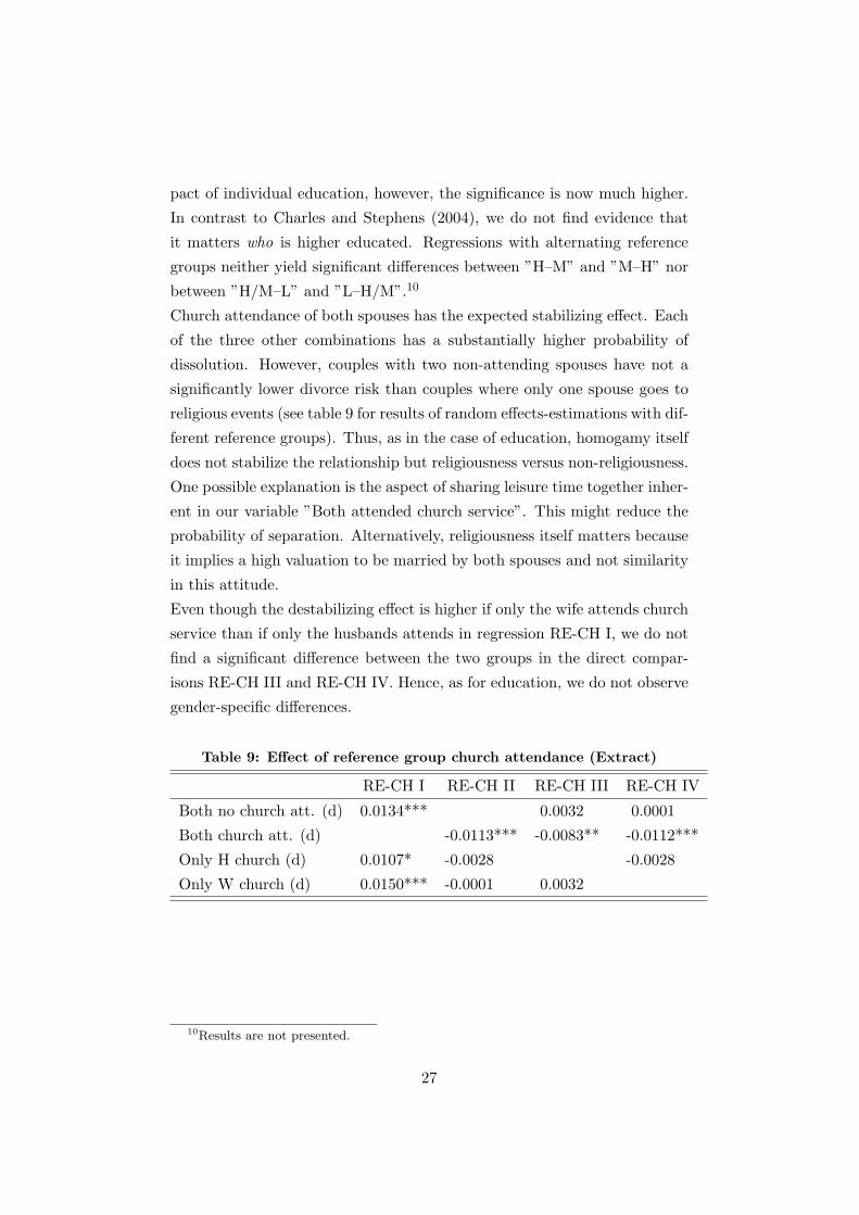
pact of individual education, however, the significance is now much higher.
In contrast to Charles and Stephens (2004), we do not find evidence that
it matters who is higher educated. Regressions with alternating reference
groups neither yield significant differences between ”H–M” and ”M–H” nor
between ”H/M–L” and ”L–H/M”.10
Church attendance of both spouses has the expected stabilizing effect. Each
of the three other combinations has a substantially higher probability of
dissolution. However, couples with two non-attending spouses have not a
significantly lower divorce risk than couples where only one spouse goes to
religious events (see table 9 for results of random effects-estimations with dif-
ferent reference groups). Thus, as in the case of education, homogamy itself
does not stabilize the relationship but religiousness versus non-religiousness.
One possible explanation is the aspect of sharing leisure time together inher-
ent in our variable ”Both attended church service”. This might reduce the
probability of separation. Alternatively, religiousness itself matters because
it implies a high valuation to be married by both spouses and not similarity
in this attitude.
Even though the destabilizing effect is higher if only the wife attends church
service than if only the husbands attends in regression RE-CH I, we do not
find a significant difference between the two groups in the direct compar-
isons RE-CH III and RE-CH IV. Hence, as for education, we do not observe
gender-specific differences.
Table 9: Effect of reference group church attendance (Extract)
RE-CH I RE-CH II RE-CH III RE-CH IV
Both no church att. (d) 0.0134*** 0.0032 0.0001
Both church att. (d) -0.0113*** -0.0083** -0.0112***
Only H church (d) 0.0107* -0.0028 -0.0028
Only W church (d) 0.0150*** -0.0001 0.0032
10Results are not presented.
27

6 Conclusions
Using a rich panel data set on German couples, we test the hypothesis that
homogamy increases marital stability. Becker assumes that earnings ca-
pacities should be dissimilar but traits like intelligence, age, religion, and
education should be positively correlated.
We put an emphasis on education and religiousness measured by attendance
of church services and other religious events. Education is affected by intelli-
gence and preferences concerning the division of labor within the marriage.
On the other hand, income prospects also depend on education. Hence,
educational attainment may affect the stability of a relationship in multi-
ple ways. Religious affiliation expresses views concerning the importance of
marriage. As we have information for both spouses on that we can test for
the effects of similarity and dissimilarity of preferences.
Our cloglog estimations, considering also couple-specific unobserved hetero-
geneity, do not generally show that two spouses who are similar to each
other have a lower risk of divorce than dissimilar spouses. A stabilizing ef-
fect of homogamy can be found for age: the risk of divorce increases with
increasing age difference. In contrast, a stabilizing effect with respect to
education and church attendance can only be found for certain groups like
couples with two medium- or two high-educated spouses, or if both attend
religious events. Our results suggest that not the combination matters but
low versus medium or high level education and church attendance of both
spouses versus no church attendance of at least one spouse. Spouses with a
low educational level and couples without religious affiliation realize signifi-
cantly higher divorce risks. Therefore, other aspects of these characteristics
and activities seem to play an important role. Examples are sharing leisure
time together or the ability to form expectations.
So far, we have neglected important financial aspects in addition to house-
hold’s total net income. It is, nevertheless, very likely that not only hours
worked but the associated individual wage as well as non-labor income and
property influence the success of a relationship.
28

A Descriptive statistics
Table 10: Descriptive statistics of explanatory variables
Variable Mean Std. Dev.
For at least one spouse not first marriage 0.35 0.48
H: Age at marriage 32.19 8.28
W: Age at marriage 29.43 7.43
Absolute age difference 4.06 3.98
H: Year of birth 1960 9.05
W: Year of birth 1962 8.17
Live in city center 0.09 0.28
No. of HH members age 0–1 0.14 0.36
No. of HH members age 2–7 0.57 0.75
No. of HH members age 8–15 0.39 0.71
Household’s net income in 1,000 Euro of 2002 2.64 1.30
H: Cum. number of months in UE 5.41 14.52
W: Cum. number of months in UE 5.41 10.75
H: Hours worked (per week) in t-3 40.13 14.19
W: Hours worked (per week) in t-3 19.41 17.51
1)”H:” stands for husbands, ”W:” for wives, ”HH” for household, ”UE” for
unemployment.
2) All variables refer to period t-1 except hours worked.
B Definition of hours worked
Figures 2 and 3 show the development of average hours worked in the years
preceding divorce. The figures for divorced wives and divorced husbands
refer to the average hours worked of those couples that eventually divorce,
but while they are still married. Only the short-dashed lines give the mean
of all female and male observations, respectively. It becomes obvious that
wives and husbands that eventually divorce work generally more on average
than the pool of all wives and husbands. However, the difference is almost
negligible for husbands. For both sexes, we observe a change in working
behavior prior to divorce. Husbands work less while wives widen their labor
29

supply. In either case, the period-specific mean crosses the average of the
divorced between t − 4 and t − 3. Therefore, we use data of t − 3 for our
regressions to diminish the endogeneity problem.
Nevertheless, we tested the effect of the definition of hours worked on our
variables of interest. Tables 11 and 12 compare the marginal effects of
random effects estimations if hours worked of different periods from t − 1
to t − 5 are used. We can see that the results are only slightly affected by
the definition of hours worked. Not surprisingly, the biggest changes can be
observed in the effects of children. The impact of new-born children in t− 1
is insignificant if hours worked of period t−1 is included. With labor supply
of later periods, the effect becomes larger and significant. Apparently, this
children-variable captures partly the effect of a non-working wife in period
t− 1.
Figure 2: Means of husbands’ hours worked in years prior to divorce
3839
4041
42M
eans
of h
usba
nds’
hou
rs w
orke
d
−10 −9 −8 −7 −6 −5 −4 −3 −2 −1Years prior to divorce
Period−specific means divorced husbandsOverall mean divorced husbandsOverall mean all husbands
30

Figure 3: Means of wives’ hours worked in years prior to divorce
1416
1820
22M
eans
of w
ives
’ hou
rs w
orke
d
−10 −9 −8 −7 −6 −5 −4 −3 −2 −1Years prior to divorce
Period−specific means divorced wivesOverall mean divorced wivesOverall mean all wives
31

Table 11: Effect period hours worked on RE estimations I
H Ia H IIa H IIIa H IVa H VaNot first marriage -0.0015 -0.0015 -0.0015 -0.0014 -0.0013H: Age at marriage -0.0004 -0.0004 -0.0005 -0.0005 -0.0005W: Age at marriage 0.0002 0.0003 0.0003 0.0002 0.0002Age difference 0.0007** 0.0007** 0.0007** 0.0007** 0.0007**H: Year of birth -0.0001 -0.0001 -0.0002 -0.0002 -0.0001W: Year of birth 0.0003 0.0003 0.0003 0.0003 0.0002No. of HH mem. 0–1 -0.0060 -0.0089** -0.0101** -0.0101** -0.0102**No. of HH mem. 2–7 0.0006 0.0005 -0.0001 -0.0010 -0.0015No. of HH mem. 8–15 0.0051*** 0.0049*** 0.0051*** 0.0047** 0.0043**Live in City 0.0095** 0.0096** 0.0099** 0.0102** 0.0102**HH net income 0.0009 0.0008 0.0013 0.0012 0.0012H: High-educated -0.0064* -0.0069** -0.0072** -0.0073** -0.0071**H: Medium-educated -0.0050 -0.0055 -0.0055 -0.0054 -0.0052W: High-educated -0.0068** -0.0064** -0.0062* -0.0060* -0.0060*W: Medium-educated -0.0080** -0.0078** -0.0079** -0.0076** -0.0075**H: No church att. 0.0082*** 0.0082*** 0.0086*** 0.0087*** 0.0088***W: No church att. 0.0027 0.0025 0.0026 0.0027 0.0027H: No. mon. UE cum. 0.0002*** 0.0002*** 0.0002*** 0.0002*** 0.0002***W: No. mon. UE cum. 0.0001 0.0001 0.0001 0.0001 0.0001H: Hours work t-1 -0.0001W: Hours work t-1 0.0002***H: Hours work t-2 0.0001W: Hours work t-2 0.0002**H: Hours work t-3 -0.0001W: Hours work t-3 0.0001*H: Hours work t-4 0.0001W: Hours work t-4 0.0001H: Hours work t-5 0.0001W: Hours work t-5 -0.0001Rho 0.36503 0.38060 0.34589 0.35017 0.34674p-value H0 : Rho = 0 0.019 0.015 0.025 0.026 0.028Chi2 120.76 115.74 119.82 113.83 114.43
1) Table shows marginal effects computed at the mean of each covariate except for dummies.
2) *: p<0.10, **: p<0.05, ***: p<0.01; st.err. computed by the delta method.
3) ”H:” stands for husbands, ”W:” for wives, ”HH” for household.
32

Table 12: Effect period hours worked on RE estimations II (Extract)
H Ib H IIb H IIIb H IVb H Vb
H – H -0.0119*** -0.0119*** -0.0122*** -0.0119*** -0.0117***
M – M -0.0172*** -0.0175*** -0.0177*** -0.0168*** -0.0162***
H/M – L -0.0079** -0.0080** -0.0083*** -0.0079** -0.0076**
H – M -0.0120*** -0.0121*** -0.0125*** -0.0123*** -0.0121***
M – H -0.0101*** -0.0099*** -0.0100*** -0.0098*** -0.0097***
L – H/M -0.0094*** -0.0092*** -0.0095*** -0.0090*** -0.0088***
Both no church att. 0.0131*** 0.0129*** 0.0134*** 0.0136*** 0.0137***
Only H church 0.0110* 0.0104* 0.0107* 0.0111* 0.0112*
Only W church 0.0145*** 0.0145*** 0.0150*** 0.0153*** 0.0154***
H: Hours work t-1 -0.0001
W: Hours work t-1 0.0002***
H: Hours work t-2 0.0001
W: Hours work t-2 0.0002**
H: Hours work t-3 -0.0001*
W: Hours work t-3 0.0001*
H: Hours work t-4 0.0001
W: Hours work t-4 0.0001
H: Hours work t-5 0.0001
W: Hours work t-5 -0.0001
Rho 0.33659 0.35570 0.31812 0.32711 0.32493
p-value H0 : Rho = 0 0.029 0.022 0.037 0.036 0.038
Chi2 125.74 120.19 124.79 117.89 118.26
1) Table shows marginal effects computed at the mean of each covariate except for dummies.
2) *: p<0.10, **: p<0.05, ***: p<0.01; st.err. computed by the delta method.
3) ”H:” stands for husbands, ”W:” for wives.
4) First six rows refer to education. First letter stands for husband’s, second for wife’s. ”H”
denotes high education, ”M” medium, and ”L” low.
33

References
Becker, G. S. (1973). A theory of marriage: Part I. Journal of Political
Economy, 81(4):813–846.
Becker, G. S. (1974a). A theory of marriage: Part II. Journal of Political
Economy, 82(2):S11–S26.
Becker, G. S. (1974b). A theory of social interactions. Journal of Political
Economy, 82(6):1063–1093.
Becker, G. S. (1981). A Treatise on the Family. Harvard University Press.
Becker, G. S., Landes, E. M., and Michael, R. T. (1977). An economic
analysis of marital instability. Journal of Political Economy, 85(6):1141–
1187.
Binmore, K., Rubinstein, A., and Wolinsky, A. (1986). The Nash bargaining
solution in economic modelling. Rand Journal of Economics, 17(2):176–
188.
Blossfeld, H.-P. and Muller, R. (2002). Union disruption in comparative
perspective: The role of assortative partner choice and careers of couples.
International Journal of Sociology, 32(4):3–35. Guest Editor’s Introduc-
tion.
Blossfeld, H.-P. and Timm, A. (2003). Who marries whom in West Ger-
many? In Blossfeld, H.-P. and Timm, A., editors, Who marries whom?
Educational systems as marriage markets in modern societies, pages 19–
35. Kluwer Academic Publishers.
Browning, M., Bourguignon, F., Chiappori, P.-A., and Lechene, V. (1994).
Income and outcomes: A structural model of intrahousehold allocation.
Journal of Political Economy, 102(6):1067–1096.
Bumpass, L. L., Martin, T. C., and Sweet, J. A. (1991). The impact of family
background and early marital factors on marital disruption. Journal of
Family Issues, 12(1):22–42.
Bumpass, L. L. and Sweet, J. A. (1972). Differentials in marital stability:
1970. American Sociological Review, 37(6):754–766.
34

Cameron, A. C. and Trivedi, P. K. (2005). Microeconometrics. Methods and
applications. Cambridge University Press.
Charles, K. K. and Stephens, M. (2004). Job displacement, disability, and
divorce. Journal of Labor Economics, 22(2):489–522.
Diekmann, A. and Klein, T. (1991). Bestimmungsgrunde des Eheschei-
dungsrisikos. Eine empirische Untersuchung mit den Daten des
soziookonomischen Panels. Kolner Zeitschrift fur Soziologie und
Sozialpsychologie, 43(2):271–290.
Finnas, F. (1997). Social integration, heterogeneity, and divorce: The case of
the swedish-speaking population in finland. Acta Sociologica, 40(3):263–
277.
Haisken-DeNew, J. P. and Hahn, M. (2006). Panelwhiz: A flexible
modularized stata interface for accessing large scale panel data sets.
(http://www.PanelWhiz.eu). mimeo.
Hall, A. (1997). Drum prufe, wer sich ewig bindet. Eine empirische Un-
tersuchung zum Einfluss vorehelichen Zusammenlebens auf das Schei-
dungsrisiko. Zeitschrift fur Soziologie, 26(4):275–295.
Hoddinott, J. and Haddad, L. (1995). Does female income share influence
household expenditure? Evidence from Cote d’Ivoire. Oxford Bulletin of
Economics and Statistics, 57(1):77–96.
Johnson, W. R. and Skinner, J. (1986). Labor supply and marital separation.
American Economic Review, 76(3):455–469.
Kiefer, N. M. (1988). Economic duration data and hazard functions. Journal
of Economic Literature, 26(2):646–679.
Koch, A. (1993). An economic analysis of marital dissolution in West Ger-
many. Munchener wirtschaftswissenschaftliche Beitrage, 93-10.
Konrad, K. A. and Lommerud, K. E. (1995). Family policy with non-
cooperative families. Scandinavian Journal of Economics, 97(4):581–601.
Kopp, J. (2000). Socio-structural determinants of divorce: A test of some
hypotheses of the economic theory of the family. In Weesie, J. and Raub,
35

W., editors, The Management of durable relations: Theoretical models
and empirical studies of households and organizations. ThelaThesis.
Lewis, S. K. and Oppenheimer, V. K. (2000). Educational assortative mat-
ing across marriage markets: Non-hispanic whites in the united states.
Demography, 37(1):29–40.
Liu, Q. and Pierce, D. A. (1994). A note on Gauss-Hermite quadrature.
Biometrika, 81(3):624–629.
Lundberg, S. and Pollak, R. A. (1993). Separate spheres bargaining and the
marriage market. Journal of Political Economy, 101(6):988–1010.
Manser, M. and Brown, M. (1980). Marriage and household decision-making:
A bargaining analysis. International Economic Review, 21(1):31–44.
McElroy, M. B. and Horney, M. J. (1981). Nash-bargained household de-
cisions: Toward a generalization of the theory of demand. International
Economic Review, 22(2):333–349.
Meyer, B. D. (1990). Unemployment insurance and unemployment spells.
Econometrica, 58(4):757–782.
Muller, R. (2003). Union disruption in West Germany. Educational ho-
mogeneity, children, and trajectories in marital and nonmarital unions.
International Journal of Sociology, 33(2):3–35.
Nash, J. F. (1950). The bargaining problem. Econometrica, 18(2):155–162.
Nicoletti, C. and Rondinelli, C. (2006). The (mis)specification of discrete
time duration models with unobserved heterogeneity: a monte carlo study.
ISER Working Paper 2006–53.
Nielsen, H. S. and Svarer, M. (2006). Educational homogamy: Preferences
or opportunities? IZA Discussion Paper No. 2271.
Rabe-Hesketh, S. and Skrondal, A. (2008). Multilevel and longitudinal mod-
eling using Stata. Stata Press, 2nd edition.
Statistisches Bundesamt (2005). Ehescheidungen 2004. Wirtschaft und
Statistik, 12:1273–1282.
36

Sueyoshi, G. T. (1995). A class of binary response models for grouped
duration data. Journal of Applied Econometrics, 10(4):411–431.
Tzeng, J. M. and Mare, R. D. (1995). Labor market and socioeconomic
effects on marital stability. Social Science Research, 24(4):329–351.
Wagner, M. (1997). Scheidung in Ost- und Westdeutschland. Zum
Verhaltnis von Ehestabilitat und Sozialstruktur seit den 30er Jahren.
Campus Verlag.
Weiss, Y. and Willis, R. J. (1997). Match quality, new information, and
marital dissolution. Journal of Labor Economics, 15(1, part 2):S293–S329.
37