market power and relationships in small business lending

FEDERAL RESERVE BANK OF SAN FRANCISCO

WORKING PAPER SERIES

Working Paper 2007-07 http://www.frbsf.org/publications/economics/papers/2006/wp07-07bk.pdf

The views in this paper are solely the responsibility of the authors and should not be interpreted as reflecting the views of the Federal Reserve Bank of San Francisco or the Board of Governors of the Federal Reserve System.

Market Power and Relationships in Small Business Lending

Elizabeth Laderman Federal Reserve Bank of San Francisco

November 2006

Market Power and Relationships in Small Business Lending∗

Elizabeth Laderman †

Federal Reserve Bank of San Francisco

November 20, 2006

Abstract

The empirical research literature regarding the effects of market structure on small business

lending has yielded ambiguous results. This paper empirically tests for the presence of coun-

tervailing effects of increases in market concentration on small business loan volume. Coun-

tervailing effects would be expected if both the traditional Structure, Conduct, Performance

(SCP) paradigm of industrial organization and a paradigm whereby market power benefits the

formation of lending relationships (the relationship hypothesis), are at work. Using Community

Reinvestment Act (CRA) data on small loans to small businesses, it is found that, on average,

across MSAs, SCP effects dominate. But, as predicted by the relationship hypothesis, the neg-

ative effects of increases in concentration on small business loan volume are weaker, the greater

the presence of young firms and the higher the business failure rate. Relationship effects due

to business failure appear to come from highly concentrated MSAs. Endogeneity concerns are

further addressed with the estimation of a regression that separates out the effects of changes

in the number of lenders from the effects of changes in the sum of squared deviations of market

shares.

JEL Codes: G21, L11, D82

Key Words: Banking, Market Structure, Asymmetric Information, Small Business Lending

∗The views expressed herein are those of the authors and do not necessarily reflect those of the Federal ReserveBank of San Francisco or the Federal Reserve System. I would like to thank Rob Valletta, Mark Doms, and JimWilcox for very helpful comments. I thank Paul Schwabe and Jin Oh for valuable research assistance.

†Economic Research Department, 101 Market Street, MS 1130, San Francisco, CA 94105, USA. Telephone: (415)974-3171. Facsimile: (415) 974-3429. Email: [email protected].

1

mailto:[email protected]

1 Introduction

Small businesses are a vital part of the U.S. economy. According to the Small Business Admin-

istration, small businesses employ roughly half of the nation’s workers. In addition, it is thought

that small business investment plays an important role in business cycle fluctuations.

Evidence from the Federal Reserve’s 1998 Survey of Small Business Finances suggests that

bank financing is very important for small businesses, especially for young firms (Robb (2002)).1

In addition, it appears that the lending process can become disrupted as a result of bank mergers;

a 2004 survey indicated that among small businesses that have gone through a merger with their

bank, 26 percent switched their banking business to another institution (Julavits (2004)).

This paper investigates how small business loan volumes are affected by small business lending

market structure. In other bank product markets, notably mortgage lending and retail deposit

markets, researchers have found empirical evidence that higher market concentration is positively

and significantly correlated with higher prices and/or higher bank profits. (See, for example, Rosen

(2003), Pilloff and Rhoades (2002), Rhoades (1992), and Berger and Hannan (1989).)2.

Results regarding the relationship between market structure and small business lending have

been more ambiguous. Studies of the effect of bank size on small business lending have tended to

suggest that larger banks, and, by extension, more concentrated markets, are associated with less

small business lending. In contrast, direct studies of the relationship between market structure and

small business loan volumes have found that more concentrated markets are associated with more

small business lending (Zarutskie (2003) and DeYoung et al. (1999)). Studies of the effects of bank

mergers on small business lending have yielded mixed results.

This paper empirically tests for the presence of two kinds of effects of increases in concentration

on the volume of small business lending, using MSA level data collected from bank reports filed

in compliance with the Community Reinvestment Act (CRA). The first effect is the traditional1A 2004 survey by the National Federation for Independent Business Research Foundation suggested that small

businesses as a whole do not rank the ability to obtain credit high among their concerns. However, the same surveyalso suggested that young small businesses are more concerned about financing than older small businesses. (Marcuss(2004)).

2Some researchers have even linked weak competition in banking markets to real outcomes, not just financialeffects (Cetorelli (2004); Cetorelli and Strahan (2004); Garmaise and Moscowitz (2004); and Rajan and Zingales(1998))

2

Structure Conduct Performance (SCP) effect of industrial organization, whereby an increase in

market concentration decreases competition and, thereby, small business loan volume. The second

is a "relationship effect,"as modeled by Petersen and Rajan (1995): in a world with asymmetric

information and moral hazard, an increase in market power increases banks’ incentives to form

lending relationships with young firms with relatively poor prospects.

I find that, on average, across MSAs, SCP effects dominate. But, as predicted by the relationship

hypothesis, the negative effects of increases in concentration on small business loan volume are

weaker, the greater the presence of young firms in the MSA and the higher the firm failure rate.

However, results also suggest that while SCP effects and relationship effects associated with firm

age are the same no matter the level of concentration, relationship effects associated with firm

failure appear only in highly concentrated markets. Estimates based on an alternative specification

that uses the number of lenders and the sum of squared deviations of market shares instead of the

HHI support the view that the presence of SCP effects is not merely the result of endogeneity bias.

2 Related Literature

Two broad strands of literature relate to the relationship between market structure and the volume

of small business lending. One strand examines the effects of banking industry consolidation,

either indirectly, through studying the role of bank size in small business lending, or directly,

through studying the effects of mergers. Numerous researchers have found that larger banks are

less likely to lend to small businesses than smaller banks, which lends at least qualitative support

to the SCP hypothesis (Avery and Samolyk (2004), Sapienza (2002), Berger et al. (2001), and

Levonian and Soller (1996)). However, studies of the effects of mergers on small business lending

have yielded mixed results, with some evidence that mergers reduce lending to small businesses

and other evidence of the opposite. Sapienza (2002) and Avery and Samolyk (2004) find that

it is important to take account of the sizes of the merging banks. Similarly, Berger et al. (1998)

emphasize the importance of the time horizon, stressing that short-run effects of mergers may differ

from long-run effects.

Two papers have examined directly the effects of market concentration on small business loan

3

volumes, as I do in this paper. These papers suggest that, in contrast to SCP, there is a positive

correlation between concentration and small business lending. Zarutskie (2003) used balance sheet

and income statement data, including information on bank loans, as reported by a sample of young,

small corporations to the IRS. She found that increases in concentration, measured using deposits

at branches in the MSA in which the firms were headquartered, were associated with increases in

the firms’ ratios of bank debt to assets. However, this effect disappeared after the enactment of

the Riegle-Neal Interstate Banking and Branching Efficiency Act of 1994. DeYoung et al. (1999)

focused on the tendency of young banks to make small business loans and how that tendency

changes as a bank ages. However, among their results was the finding that young, small banks

make more loans under $1,000,000 when deposit market concentration increases in the MSA in

which the bank is headquartered.

Both Zarutskie and DeYoung et. al. cite a theoretical model presented by Petersen and Rajan

(1995) in support of their empirical findings. In Petersen and Rajan’s model, asymmetric infor-

mation and moral hazard generate a need for banks to build relationships with borrowers, yielding

what I will call a "relationship effect" of increases in market concentration.

Petersen and Rajan model two types of young firms—high quality young firms, who can choose

between a safe project with a certain but low return, or a risky project, with an uncertain, but

higher, return. In contrast, low quality young firms have no prospect of success at all; all of the

projects of low quality young firms return nothing. The quality of a firm is unknown to a bank,

but the probability of its being high quality is known.

Petersen and Rajan argue that banks with more market power can better afford to set the low

interest rates that are required to get high quality young firms to invest in safe projects rather than

gambling the bank’s money on risky projects. This is because banks with more market power can

better compensate for the low initial interest rate with a high rate in subsequent periods, when the

bank knows more about the firm and its projects.3 Because banks with more market power are

more likely to be able to engage in this intertemporal cross-subsidization, they can better afford to

lend to young firms with a higher probability of being low quality. Banks with market power can3Formally, Petersen and Rajan model this gain in knowledge by requiring that all period-two projects are safe

projects.

4

make their expected payoff from lending to firms that turn out to be high quality high enough to

compensate for the losses that will come from lending to firms that turn out to be low quality.

Petersen and Rajan used firm-level data from the Survey of Small Business Finances and cat-

egorical deposit market concentration measures to show that, as concentration in the MSA where

the small business is headquartered increases discontinuously from perfectly competitive levels,

interest rates for loans to young firms decline. They also find that, as firms age, the effect of

concentration on interest rates becomes less negative and then becomes positive. They point out

that, strictly speaking, their theoretical model does not necessarily predict their empirical results.

Their model predicts that concentration should be negatively correlated with loan rates only for

the lowest quality young firms, not necessarily for the average quality young firm. They do not

examine interest rates for the lowest quality young firms. In contrast, I will include measures of

small business quality as well as age in my analysis, allowing me to do just that.

In their empirical work, Petersen and Rajan find relationship effects, for younger small busi-

nesses. But, although they don’t highlight the point, their results also reveal the presence of SCP

effects, for older small businesses. The empirical presence of two countervailing effects of increases

in concentration on small business lending is consistent with the presence of ambiguity in the

empirical results of the related literature overall.

One of the purposes of this paper is to investigate whether the same dichotomy of effects of

increases in concentration that appeared in Petersen and Rajan’s work, for discrete changes in

concentration and firm level data, can be found for continuous changes in concentration and MSA

level data. It is at an aggregated level that analysis of the competitive effects of proposed bank

mergers and acquisitions takes place.4 And, if effects differ depending on the age of the small

business, what are they on average for MSAs? As Petersen and Rajan point out, their regression

estimates, all of which incorporate full age-concentration interaction effects, do not say whether, in

highly concentrated markets, the lower interest rates for younger firms are outweighed by higher

interest rates for older firms.

In addition, do effects differ also by the quality of the small business and, to adhere even more4The Federal Reserve analyzes the competitive effects of proposed bank mergers using Federal Reserve Banking

markets. For urban areas, these markets often are comparable to MSAs.

5

closely to the theoretical model as presented by Petersen and Rajan themselves, by whether the

small business is both young and poor quality? Finally, do aggregate effects differ depending on

the level of concentration.

3 Data

I will address these questions using measures of concentration based on small business loans, not

deposits. The distinction is important because smaller banks have a larger ratio of small business

loans to assets than do larger banks. In addition, smaller banks tend to have a larger ratio of

deposits to assets. Therefore, banks’ small business lending shares will not, in general, equal their

deposit market shares. In contrast to DeYoung et al. (1999), who use loans under $1 million

to any business, I use CRA reported loans under $1 million to businesses with revenues under

$1 million, thereby focusing on small loans to small businesses.5 Small loans to small businesses

are the appropriate focus for tests for the presence of relationship effects associated with market

concentration. Borrowers in my sample include partnerships and sole proprietorships, as well as

older firms, and banks are of all sizes and ages.

I use a repeated cross section of CRA small business lending data for 2003 and 2004, and

analysis of the effect of concentration on the volume of small business lending is at the Metropolitan

Statistical Area (MSA) level. On the CRA report, banks give the number and total dollar amount

of loans less than $1,000,000 to businesses with gross annual revenues less than $1,000,000 (small

business loans).6 Banks report loan totals by census tract of the headquarters of the borrower or

by the census tract where the majority of the funds are being used. I aggregate from the census

tract level to the MSA level.7 Commercial and industrial loans (loans for a business purpose that

are not secured by real estate), commercial real estate loans (loans that are secured by commercial5DeYoung et al. (1999)use data on loans under $1,000,000 from the Call Report, not from the CRA.6During the period under study here, only banks with assets of at least $250 million and banks that were in a

holding company with at least $1 billion in assets reported on the CRA. Therefore, following previous research, forbanks that do not meet the CRA reporting requirement criteria, I have estimated small business lending by MSA byusing Call Report data. Specifically, I have allocated total small business lending as reported on the Call Report todifferent MSAs in proportion to the bank’s share of the bank’s total deposits in that MSA.

7MSA designations use the 2003 Office of Management and Budget definitions. If the MSA has MetropolitanDivisions within it, the analysis is at the Metropolitan Division level.

6

real estate), and loans through a business credit card all are considered business loans for CRA

reporting purposes.8 Consistent with prior research, I exclude the loans of credit card banks from

my sample.9

The Hirschman-Herfindahl Index (HHI) is a measure of market concentration and is the sum of

squared market shares, where the market shares are expressed as percents. As mentioned above, in

contrast to prior research, I measure market shares for the HHI using small loans to small businesses

The number of small businesses is included as a control for small business loan demand. The

number of businesses, by revenue category, MSA, and year, is from Dun and Bradstreet. I also

include the population of the MSA, average annual payroll employment growth for the MSA from

1995 to 2000, and average annual payroll employment growth from year t − 2 to year t + 1 as

demand controls.10 All of these control variables are meant to reduce the standard errors of the

estimated equations. Small business counts and population also are controls for market size. The

regression equation needs controls for market size because, empirically, the HHI is highly negatively

correlated with market size, and market size is of course positively correlated with the dependent

variable.

Payroll employment growth should help reduce possible downward bias of the coefficient on

concentration by helping to control for general economic conditions. MSAs where employment

is growing more quickly may have small businesses that are growing more quickly and therefore8Banks report business credit card lines of credit , whether drawn on or not, on the CRA. In contrast, personal

credit card lines of credit, even if used for business purposes (for example, lines through a small business owner’spersonal credit card), are not reported on the CRA.

9I define credit card banks to include commercial banks that have a ratio of total consumer loans to assets of atleast 0.5 and a ratio of personal credit card loans to total consumer loans of at least 0.9, as of the fourth quarterof 2003. (As of the fourth quarter of 2001, the mean ratio of credit card loans to consumer loans across all banksreporting on the Call Report was 0.03, the median less than 0.01.) The definition of a credit card bank also includesany bank that has a ratio of personal credit card loans to consumer loans of at least 0.9 and meets at least one of thefollowing criteria: it is reported by the Nilson Report as being among the top 50 banks in terms of credit card loansoutstanding in 2003 or its main activity, as indicated by the Federal Reserve’s National Information Center, is creditcard issuance.

In addition, I define as credit card banks these banks that are reported by the Nilson Report as being among thetop 50: Chase Manhattan Bank U.S.A., N.A., DE (ratio of credit card loans to consumer loans of 0.8) and MBNAAmerica Bank, N.A., DE (0.7).

Finally, based on conversations with representatives of the following institutions or state government supervisoryagency representatives, I exclude these additional "business credit card" banks: MBNA America Delaware, N.A., DE;Universal Financial Corporation, UT; Mill Creek Bank, UT; Advanta Bank Corp., UT; Volvo Commercial CreditCorp., Utah, UT; Wright Express FS Corp., UT; Pitney Bowes Bank, UT; and Capital One, F.S.B., VA.

10MSA population figures are estimates for year t.

7

seeking more bank financing. At the same time, MSAs where employment is growing more quickly

may attract bank entry, which would tend to decrease concentration. Employment growth from

1995 to 2000 is a relatively long-term average that excludes the March-November 2001 recession.

Employment growth from year t − 2 to t + 1 reflects more current economic conditions as well as

incorporating a forward looking element to capture small firms’ views of likely business prospects

into the near-term future.

I also include the size of small businesses and the age of small businesses as demand-side control

variables. Bitler et al. (2001) present evidence from the Federal Reserve System’s Survey of Small

Business Finances (SSBF) that small businesses with annual revenue greater than $50,000 are more

likely to have a bank relationship. (The size of small businesses also is a scale variable.) In addition,

the SSBF indicates that small businesses with a current owner tenure of more than four years are

more likely to have a bank relationship.11 I use the Dun and Bradstreet business counts by revenue

subcategory of under $1,000,000 and the Dun and Bradstreet business counts by revenue, current

owner tenure, MSA, and year to measure small business size and age, respectively. I also use the

Dun and Bradstreet business counts by years since incorporation, MSA, and year to measure firm

age.12

I include a number of variables to test for the presence of relationship effects. As just men-

tioned, firm age variables are included as demand-side control variables. When I am testing for

relationship effects, these variables also enter interacted with concentration. The proxies for firm

quality that I use are the MSA unemployment rate, the MSA business failure rate, and a dummy

variable indicating whether the MSA is in the bottom quartile of the MSA median family income

distribution. I derive the business failure rate from the Dun and Bradstreet data.13

To address remaining concerns regarding the possible endogeneity of market concentration, I

also estimate equations which exclude the HHI, but include the number of lenders and the sum of11It is noted that the Survey of Small Business Finances definition of a small business is fewer than 500 employees,

rather than the CRA definition of annual revenue less than $1,000,000.12The Dun and Bradstreet data do not include information on years since incorporation for small businesses, only

for all businesses.13The Dun and Bradstreet data give business counts by years since incorporation category, MSA, and year. The

category indicating the youngest firms is firms zero to four years old. By assuming constant annual business formationrates and failure rates for each MSA between 2000 and 2004, I am able to use the business counts in 2003 and 2004and the number of businesses that are zero to four years old in 2004 to back out the firm failure rate for each MSA.

8

squared deviations of market shares separately. I discuss this further in the next section.

Sample statistics are shown in Table 1.

4 Regression Specifications

4.1 Baseline Regressions

The dependent variable, SBL, is the log of the dollar volume of small business loans. All variables

are measured at the MSA level for year t. The main baseline regression, estimated using OLS, is:

SBL = α + β1HHI + β2SB + β3LGSB + β4POP + β5PEG9500

+ β6PEG3Y + β7FIRM AGE + ε,

(4.1)

where HHIis the Hirschman-Herfindahl Index, SB is the log of the number of small businesses,

LGSB is the proportion of small businesses with gross annual revenue of at least $50,000, POP

is the log of population, PEG9500 is the average annual employment growth rate from 1995 to

2000, PEG3Y is the average annual employment growth rate from year t − 2 to year t + 1, and

FIRM AGE is the proportion of small businesses with current owner tenure of less than five years

or the proportion of all businesses incorporated less than five years.

To test for robustness of the results to inclusion of firm quality variables, a second baseline

regression includes, in addition to the variables in equation (4.1), FIRM QUALITY :


+ β6PEG3Y + β7FIRM AGE + β8FIRM QUALITY + ε.

(4.2)

FIRM QUALITY is the unemployment rate, the firm failure rate, or a dummy variable indi-

cating that the MSA is in the lowest quartile for median family income.

4.2 Tests for relationship effects

I estimate three types of regression equations to test for the presence of relationship effects. The first

type tests for the presence of relationship effects due solely to firm age. In their paper, Petersen and

9

Rajan tested for the presence of relationship effects due solely to firm age. This type of regression

takes the form:


+ β6PEG3Y + β7FIRM AGE + β8 (FIRMAGE) (HHI) + ε.

(4.3)

The second type of regression tests for the presence of relationship effects due to firm age and

to firm quality. This type of regression takes the form:


+ β6PEG3Y + β7FIRM AGE + β8 (FIRMAGE) (HHI)

+ β9FIRM QUALITY + β10 (FIRMQUALITY ) (HHI) + ε.

(4.4)

Following Petersen and Rajan’s theoretical model, which emphasizes that relationship effects

pertain to firms that are young and low quality, the third type of regression takes the form:


+ β6PEG3Y + β7FIRM AGE + β8FIRM QUALITY

+ β9Y LQ + β10 (Y LQ) (HHI) + ε,

(4.5)

where Y LQ is a dummy variable indicating that the MSA is in the top quartile for FIRM AGE

and, when FIRM QUALITY is the unemployment rate or the firm failure rate, is also in the

top quartile for FIRM QUALITY . (Recall that FIRM AGE and FIRMQUALITY actually

measure youth and low quality, increasing in value as firms become younger and as their quality

deteriorates, respectively.) When FIRM QUALITY is a dummy variable indicating whether or not

the MSA is in the lowest quartile for median family income, Y LQ requires that that dummy variable

equals one. Note that, in addition to Y LQ, I include both FIRM AGE and FIRM QUALITY

by themselves. This is because, as will be seen from the results shown below, FIRM AGE and

FIRM QUALITY are almost always statistically significant. Y LQ is included by itself in addition

to in interaction with HHI so that any intercept shift resulting from Y LQ being equal to one is not

10

erroneously attributed to a change in the slope with respect to HHI. In addition, the inclusion of

Y LQ by itself is analogous to the inclusion of FIRM AGE and FIRM QUALITY by themselves

in equations (4.3)and (4.4).

4.3 Tests for differential effects by concentration level

Marginal effects of increases in concentration on small business lending may be different in uncon-

centrated or moderately concentrated markets than in highly concentrated markets. For example,

if there are very many lenders in the market and concentration is relatively low, one might suspect

that small increases in concentration would affect small business lending very little, either through

SCP or through relationship effects.

To test for differences in effects by level of concentration, I estimate a set of regressions using

a dummy variable indicating whether the market is "highly concentrated," as defined by the De-

partment of Justice. This dummy variable, HIHHI, is one if HHI >= 1, 800. The specification

to test for differences in average effects is:

SBL = α + β1HHI + β2HIHHI + β3 (HHI) (HIHHI) + β4SB + β5LGSB

+ β6POP + β7PEG9500 + β8PEG3Y + β9FIRMAGE + ε.

(4.6)

The second specification allows for full FIRM AGE and firm quality interaction effects:

SBL = α + β1HHI + β2HIHHI + β3 (HHI) (HIHHI) + β4SB + β5LGSB

+ β6POP + β7PEG9500 + β8PEG3Y + β9FIRMAGE

+ β10 (FIRM AGE) (HHI) + β11 (FIRM AGE) (HIHHI)

+ β12 (FIRMAGE) (HHI) (HIHHI) + β13FIRMQUALITY

+ β14 (FIRM QUALITY ) (HHI) + β15 (FIRM QUALITY ) (HIHHI)

+ β16 (FIRM QUALITY ) (HHI) (HIHHI) + ε.

(4.7)

11

4.4 Tests of share distribution effects by concentration level

As mentioned in the last section, the inclusion of the demand control variables PEG9500 and

PEG3Y should help reduce possible downward bias of the coefficient on concentration.

To address remaining concerns regarding the possible endogeneity of market concentration, I

also estimate equations which exclude the HHI, but, using the formula for the HHI, include the

number of lenders and the sum of squared deviations of market shares separately. Changes in

the distribution of market shares, holding the number of lenders constant, may be less subject to

endogeneity concerns. In particular, Ericson and Pakes (1995) present a model of industry dynamics

in which entry, exit, investment, and idiosyncratic shocks result in equilibria with heterogeneous

firm sizes. Different shocks in different markets could provide an exogenous source of variation in

concentration, even if the number of lenders is held constant.14

To separate out the effects of changes in the number of lenders from changes in deviations of

market shares from the mean, I use the formula for the HHI:

HHI =n∑

i=1

x2i , (4.8)

where xi is the market share of bank i, expressed as a percent, in a market with n lenders, and

note that the sum of squared deviations of market shares from the mean is:

n∑i=1

(xi − x)2 =n∑

i=1

(x2

i

)− nx2 = HHI − 10, 000

n. (4.9)

The regression to test the for the average effect of changes in the sum of squared deviations on

small business loan volume is:

SBL = α + β1SSD + β2SCALE FACTOR + β3SB + β4LGSB + β5POP

+ β6PEG9500 + β7PEG3Y + β8FIRM AGE + ε,

(4.10)

14Correlations between HHI and PEG9500 (-.19) and between SSD and PEG9500 (-.15), for example, are bothrelatively low, but not completely negligible. However, within number of lender quartiles, the correlations betweenSSD and PEG9500 are neither as large nor even consistently negative. From smallest to largest MSA, by numberof lenders, these correlations are -.01, -.13, .06, and .11.

12

where SSD is the sum of squared deviations of the banks’ market shares from the mean and

SCALE FACTOR is 10, 000/n.

I also estimate a set of equations with full firm age and quality interaction effects:

SBL = α + β1SSD + β2SCALE FACTOR + β3SB + β4LGSB + β5POP

+ β6PEG9500 + β7PEG3Y + β8FIRM AGE

+ β9 (FIRM AGE) (SSD) + β10 (FIRM AGE) (SCALE FACTOR)

+ β11FIRM QUALITY + β12 (FIRM QUALITY ) (SSD)

+ β13 (FIRM QUALITY ) (SCALE FACTOR) + epsilon.

(4.11)

5 Regression Results

5.1 Baseline Results

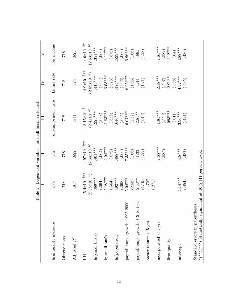
Regression results for equations (4.1) and (4.2) show that, on average, HHI has a negative and

almost always at least marginally statistically significant effect on small business loan volumes.

(Table 2.) Controlling for just firm age (columns I and II), a 100 point increase in the HHI

decreases small business loan volume by about half a percent. The one exception to statistical

significance of the HHI coefficient in Table 2 is in column III, where firm quality is measured by the

unemployment rate. As will be seen in Table 6, however, when the coefficient on HHI is allowed

to vary by both years since incorporation and the unemployment rate, the coefficient on HHI by

itself is statistically significant.

The coefficients on most of the demand control variables are highly statistically significant

and of the expected sign. However, the sign on small business size is, unexpectedly, negative.

This may indicate a substitution effect, wherein larger small businesses are more likely to have

other financing options besides bank loans.15 Similarly, the negative coefficient on the three-year

employment growth rate may be due to greater opportunity for alternative financing options in

stronger economies. There also is anecdotal evidence that small businesses may lose employees to15This is not inconsistent with the SSBF, as long as access to non-bank sources of credit increases more than

access to bank credit as a small business grows.

13

larger businesses in economic booms.16.

The coefficients on owner tenure, years since incorporation, unemployment, the firm failure rate,

and the median family income variable all are negative and statistically significant, lending support

to their roles as age and quality measures for purposes of empirical tests for relationship effects.

The negative signs on the age variables also are consistent with the SSBF.

5.2 Relationship Effects

Consistent with Petersen and Rajan, as the proportion of young firms in the MSA increases, the

marginal effect of an increase in concentration on the volume of small business lending becomes less

negative and eventually turns positive. (Table 3.)For example, using owner tenure to measure firm

age, concentration increases the volume of small business lending if more than about 11% of the

small businesses have a current owner tenure of less than five years. About 29% of the MSAs meet

this criterion. But, at the sample mean for owner tenure, an increase in concentration decreases

small business loan volume–a 100 point increase in HHI decreases lending about 0.4%.

There also is some evidence that, controlling for the number of small businesses, increases

in concentration may indeed be associated with a greater proportion of young small businesses.

Numerically, the opposite result is found for the smaller, more concentrated markets, but the

differences between within-subsample means in those cases are not statistically significant. When

the difference of means is statistically significant, for the third quartile, it is the right sign. (Table 4.)

When firm quality also is allowed to influence the coefficient on concentration, the relationship

effect due to age remains and an additional statistically significant relationship effect, due to the

firm failure rate, also appears. (Tables 5 and 6.) Now, using owner tenure to measure firm age, the

estimates in column II of Table 5 indicate about 33% of the MSAs see increases in small business

loan volumes with increases in market concentration.

Given the above results, it is not surprising that statistically significant relationship effects due

to firms being young and low quality also are evident. (Tables 7 and 8.)16In reference to the San Francisco BayArea: ". . . the slow but steady growth in the Bay Area is ideal for

small firms, which have trouble hiring qualified people when the job market gets too hot and employees start eyeingcorporate jobs with fatter paychecks and richer benefits." (Abate (2005))

14

5.3 Differential Effects by Level of Concentration

There is no statistically significant difference between the average effects of increases in concen-

tration in markets that are highly concentrated versus those that are not. In addition, when full

firm age and quality interaction effects are allowed, there is no statistically significant difference in

age-related relationship effects by HHI level. (Table 9.)

However, relationship effects due to the firm failure rate are marginally statistically significantly

stronger when HHI is at least 1,800 than when it is below that level. (Table 9 shows results for

relationship effects using years since incorporation to measure firm age. Results using owner tenure

are qualitatively similar, including the sign and level of statistical significance of the coefficient on

the firm failure rate interacted with HHI and HIHHI.) Not only is the coefficient when HHI

is high statistically significantly greater than when it is not, it turns out that the coefficient when

HHI is high is statistically significantly greater than zero, at the one percent level. (Not shown.)

As seen in Table 9, the coefficient on the firm failure rate interacted with HHI is not statistically

significantly greater than zero when HHI is less than 1,800. Therefore, it appears that the quality-

related relationship effects seen in the sample overall are due to effects present only when HHI is

high.

The lack of a statistically significant difference in average effects of HHI between higher and

lower HHI markets may be partially due to sample differences pertaining to firm age. As seen in

Table 4, when the number of small businesses is not held constant, the proportion of young firms

appears to be higher in less concentrated markets. With apparently equal relationship effects due to

firm age in lower versus higher HHI markets, this sample difference would tend to make the average

effect of increases in concentration on small business lending less negative in lower versus higher

HHI markets. It turns out that the mean firm failure rate is very nearly the same in lower (.024)

versus higher (.022) HHI markets, and the difference is not statistically significant. Given this near

equality in firm failure rates, the presence of an extra relationship effect, due to firm quality, when

the HHI is at least 1,800, counteracts any tendency, just noted, for relationship effects due to firm

age to be stronger, and therefore for average HHI effects to be less negative, when the HHI is less

than 1,800 than when it is higher.

15

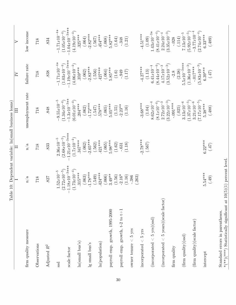
5.4 Share Distribution Effects

As explained above, I estimate effects of increases in the sum of squared deviations of market

shares on small business lending only as a robustness check on the findings indicating the presence

of statistically significant SCP effects.

Using the baseline specification of equation (4.10), the coefficient on SSD is positive but not

statistically significant. However, when full interaction with relationship effects is allowed, the

coefficient on SSD turns negative and becomes marginally statistically significant when either the

firm failure rate or median family income are used as firm quality proxies.17 (Table 10. Results using

owner tenure to measure firm age are not shown in Table 10. When owner tenure is used instead

of years since incorporation, only the specification using the firm failure rate shows a statistically

significant coefficient on SSD, but it is significant at the one percent level.)

The presence of negative and statistically significant coefficients on SSD in some specifications

supports the view that the SCP effects seen when HHI is used to measure market concentration are

not merely due to a negative correlation between HHI and omitted factors that increase the demand

for small business loans. Such correlations would be most likely to work through bank entry and

exit, and these specifications control for the number of lenders. The statistical significance of the

coefficient on SSD is notable, given that equation (4.11) does not have as much structure imposed

on it as the regressions with HHI. As can be seen from equation (4.9), the specifications with

HHI are equivalent to specifications with SSD and SCALE FACTOR in which the coefficients

on those two variables are restricted to be the same and the two variables are thus simply summed

and collapsed into one variable, HHI.

6 Conclusion

OLS regressions for MSAs for 2003 and 2004 show that, on average, increases in concentration, as

measured by small loans to small businesses, have a negative and statistically significant effect on17With years since incorporation used to measure firm age and the firm failure rate used to measure firm quality,

the estimates in Table 10 indicate that an increase in SSD, holding SCALE FACTOR constant, would decreasesmall business loan volume in about 39% of the MSAs.

16

small business loan volumes. This indicates the presence of a traditional structure, conduct, per-

formance effect from increasing market concentration. A number of demand-side control variables,

including, in particular, two employment growth rates, are included in the regression to try to

control for possible endogeneity of the HHI. In addition, estimation of an alternative specification,

using the number of lenders and the sum of squared deviations of market shares instead of the HHI,

further supports the view that the presence of statistically significant SCP effects is not solely due

to endogeneity bias.

Regression results also suggest the presence of relationship effects in connection with increases

in market concentration. The idea here, from Petersen and Rajan (1995), is that banks with more

market power can better afford to take a gamble on young firms with poor prospects because such

banks can raise their interest rates in subsequent periods. If firms are young enough or firm failure

rates are high enough, as they are for part of the sample, increases in concentration may increase

small business loan volume. It appears, however, that it is just the highly concentrated markets

that are contributing to the existence of relationship effects in connection with firm quality.

The SCP effects seen on average appear to have some economic significance, at least when

judged in relation to the effects of the other important economic conditions variable, employment

growth. On average, an HHI increase of 100 decreases lending about 0.5%. (Table 2, Columns I and

II.) However, this decrease in loan volume is comparable to that engendered by a similar magnitude

decrease (about one-seventh of a standard deviation) in the 1995-2000 payroll employment growth

rate—between 0.9% and 1.3%, as indicated by the same regression estimates.

If a given reduction in bank loans has differential effects for younger/poorer quality small

businesses than for older/higher quality small businesses, then the welfare implications of the

results presented here are unclear. For example, if younger firms (or firms with poorer prospects if

concentration is high) are more dependent on bank loans than are older, survivor firms, the average

reduction in small business loan volume that arises when concentration increases may hide a net

decline in overall welfare even when there are relatively few young firms. On the other hand, if an

insufficient proportion of young firms is destined to survive, anyway, reductions in bank financing

for such firms may not, in fact, be as detrimental to welfare as reductions in bank financing for

17

established, successful small businesses.

Despite these caveats, the results presented in this paper suggest that the exercise of regulatory

policy affecting concentration in bank small business lending likely is of at least a small amount

of real consequence and that, although, in most instances, the traditional concerns with market

power that arise out of SCP should predominate, regulators should be aware of the possibility of

countervailing benefits for young small businesses or those with relatively poor prospects.

18

7 References

Abate, T., November 28, 2005. Bay Area nears 200,000 small businesses. San Francisco Chronicle,

C8.

Avery, R. B., Samolyk, K. A., April/June 2004. Bank consolidation and small business lending:

The role of community banks. Journal of Financial Services Research 25 (2/3), 291–325.

Berger, A. N., Hannan, T., 1989. The price-concentration relationship in banking. Review of Eco-

nomics and Statistics 71 (2), 291–299.

Berger, A. N., Klapper, L. F., Udell, G. F., December 2001. The ability of banks to lend to

informationally opaque small businesses. Journal of Banking and Finance 25 (12), 2127–2167.

Berger, A. N., Saunders, A., Scalise, J. M., Udell, G. F., 1998. The effects of bank mergers and

acquisitions on small businesses lending. Journal of Financial Economics 50, 187–229.

Bitler, M. P., Robb, A. M., Wolken, J. D., 2001. Financial services used by small businesses:

Evidence from the 1998 Survey of Small Business Finances. Federal Reserve Bulletin 87 (4),

183–205.

Cetorelli, N., June part 2 2004. Real effects of bank competition.

Cetorelli, N., Strahan, P. E., October 2004. Finance as a barrier to entry: Bank competition

and industry structure in local U.S. markets. Tech. Rep. 10832, National Bureau of Economic

Research.

DeYoung, R., Goldberg, L. G., White, L. J., 1999. Youth, adolescence, and maturity of banks:

Credit availability to small businesses in an era of bank consolidation. Journal of Banking and

Finance 23, 463–492.

Garmaise, M. J., Moscowitz, T. J., December 2004. Bank mergers and crime: The real and social

effects of credit market competition. Tech. Rep. 11006, National Bureau of Economic Research.

19

Julavits, R., June 2, 2004. Sensitivity to takeovers acute for small businesses. American Banker

169 (105), 1.

Levonian, M., Soller, J., January 12, 1996. Small banks, small loans, small businesses. Federal

Reserve Bank of San Francisco Weekly Letter 96 (2).

Marcuss, M., Fall 2004. Are small businesses concerned about credit? Federal Reserve Bank of

Boston Communities and Banking, 22–24.

Petersen, M. A., Rajan, R. G., May 1995. The effect of credit market competition on lending

relationships. Quarterly Journal of Economics 110 (2), 407–443.

Pilloff, S. J., Rhoades, S. A., 2002. Structure and profitability in banking markets. Review of

Industrial Organization 20, 81–98.

Rajan, R. G., Zingales, L., 1998. Financial dependence and growth. American Economic Review

88 (3), 559–586.

Rhoades, S. A., 1992. Evidence on the size of banking markets from mortgage loan rates in twenty

cities. Federal Reserve Bulletin 78, 117–118.

Robb, A. M., 2002. Small business financing: Differences between young and old firms. Journal of

Entrepreneurial Finance and Business Ventures 7 (2), 45–65.

Rosen, R. J., November 2003. Banking market conditions and deposit interest rates. Tech. Rep. 19,

Federal Reserve Bank of Chicago.

Sapienza, P., February 2002. The effects of banking mergers on loan contracts. Journal of Finance

58 (1), 329–367.

Zarutskie, R., 2003. Does bank competition affect how much firms can borrow? New evidence from

the U.S. In: Proceedings of the 39th Annual Conference on Bank Structure and Competition.

Conference on Bank Structure and Competition. Federal Reserve Bank of Chicago, Chicago, IL,

pp. 121–136.

20

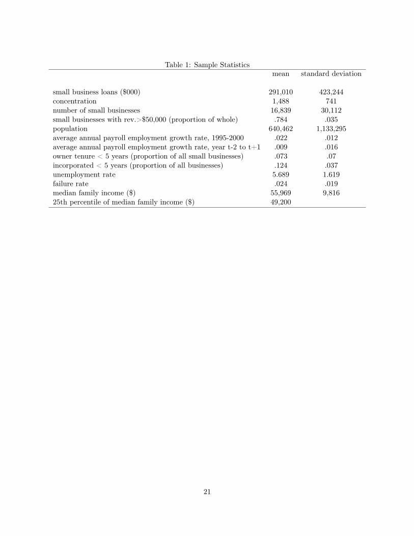
Table 1: Sample Statisticsmean standard deviation

small business loans ($000) 291,010 423,244concentration 1,488 741number of small businesses 16,839 30,112small businesses with rev.>$50,000 (proportion of whole) .784 .035population 640,462 1,133,295average annual payroll employment growth rate, 1995-2000 .022 .012average annual payroll employment growth rate, year t-2 to t+1 .009 .016owner tenure < 5 years (proportion of all small businesses) .073 .07incorporated < 5 years (proportion of all businesses) .124 .037unemployment rate 5.689 1.619failure rate .024 .019median family income ($) 55,969 9,81625th percentile of median family income ($) 49,200

21

Tab

le2:

Dep

ende

ntva

riab

le:

ln(s

mal

lbus

ines

slo

ans)

III

III

IVV

firm

qual

ity

mea

sure

n/a

n/a

unem

ploy

men

tra

tefa

ilure

rate

low

inco

me

Obs

erva

tion

s71

871

871

871

871

8

Adj

uste

dR

2.8

17.8

22.8

41.8

24.8

23

HH

I−

5.4x

10−

5**

−.4

.97x

10−

5**

−3.

15x10

−5

−.4

.9x10

−5**

−.4

.6x10

−5*

(2.5

8x10

−5)

(2.5

4x10

−5)

(2.4

x10

−5)

(2.5

2x10

−5)

(2.5

3x10

−5)

ln(s

mal

lbus

’s)

.369

***

.401

***

.225

***

.418

***

.351

***

(.06

4)(.

064)

(.06

3)(.

064)

(.06

6)lg

smal

lbus

’s-2

.08*

**-2

.94*

**-1

.83*

**-3

.03*

**-3

.11*

**(.

564)

(.57

9)(.

558)

(.57

5)(.

579)

ln(p

opul

atio

n).4

92**

*.4

88**

*.6

46**

*.4

75**

*.5

29**

*(.

068)

(.06

6)(.

065)

(.06

6)(.

066)

payr

olle

mp.

grow

th,1

995-

2000

5.04

***

7.35

***

6.07

***

6.95

***

6.96

***

(2.5

8)(1

.66)

(1.5

7)(1

.65)

(1.6

6)pa

yrol

lem

p.gr

owth

,t-2

tot+

1-2

.68*

*-1

.33

-2.8

1**

-1.4

4-.6

61(1

.19)

(1.2

2)(1

.16)

(1.2

1)(1

.23)

owne

rte

nure

<5

yrs

-.472

*(.

271)

inco

rpor

ated

<5

yrs

-2.6

5***

-1.8

1***

-2.1

8***

-2.6

1***

(.58

5)(.

559)

(.59

7)(.

582)

firm

qual

ity

-.093

***

-2.9

***

-.112

***

(.01

)(.

858)

(.04

)in

terc

ept

4.14

***

4.8*

**3.

96**

*4.

92**

*4.

88**

*(.

454)

(.43

7)(.

421)

(.43

5)(.

436)

Stan

dard

erro

rsin

pare

nthe

ses.

*(**

)(**

*)St

atis

tica

llysi

gnifi

cant

at10

(5)(

1)pe

rcen

tle

vel.

22

Table 3: Dependent variable: ln(small business loans)I II

Observations 718 718

Adjusted R2 .819 .823

HHI −1.07x10−4*** −2.43x10−4***(3.23x10−5) (8.2x10−5)

ln(small bus’s) .378*** .41***(.064) (.064)

lg small bus’s -2.07*** -2.94***(.561) (.576)

ln(population) .494*** .484***(.067) (.066)

payroll emp. growth, 1995-2000 4.93*** 7.24***(1.58) (1.65)

payroll emp. growth, t-2 to t+1 -2.87** -1.52(1.19) (1.22)

owner tenure < 5 yrs -1.86***(.579)

(owner tenure < 5 yrs)(HHI) 9.36x10−4***(3.45x10−4)

incorporated < 5 yrs -4.92***(1.09)

(incorporated < 5 yrs)(HHI) 1.62x10−3***(6.55x10−4)

intercept 4.11*** 5.05***(.452) (.447)

Standard errors in parentheses.**(***) Statistically significant at 5(1) percent level.

23

Table 4: Percent of Businesses Incorporated Less Than Five Years

Number of Small Businesses

lowest quartileHHI<mean HHI=2,032 10.8HHI>=mean HHI=2,032 10.5

second quartileHHI<mean HHI=1,632 11.7HHI>=mean HHI=1,632 11.6

third quartileHHI<mean HHI=1,417 12.8HHI>=mean HHI=1,417 13.9*

highest quartileHHI<mean HHI=877 13.6HHI>=mean HHI=877 14.4

*Statistically significant difference of means, at 10 percent level.

24

Table 5: Dependent variable: ln(small business loans)I II III

firm quality measure unemployment rate failure rate low income

Observations 718 718 718

Adjusted R2 .84 .827 .82

HHI −8.93x10−5 −1.42x10−4*** −9.92x10−5***(6.61x10−5) (3.51x10−5) (3.48x10−5)

ln(small bus’s) .203*** .404*** .327***(.063) (.064) (.066)

lg small bus’s -1.17** -2.45*** -2.28***(.535) (.561) (.564)

ln(population) .662*** .475*** .537***(.065) (.067) (.069)

payroll emp. growth, 1995-2000 4.56*** 4.86*** 4.58***(1.48) (1.56) (1.59)

payroll emp. growth, t-2 to t+1 -3.81*** -3.01*** -2.3*(1.12) (1.17) (1.2)

owner tenure < 5 yrs -1.56*** -1.06* -1.84***(.545) (.62) (.583)

(owner tenure < 5 yrs)(HHI) 7.29x10−4** 6.26x10−4* 9.87x10−4***(3.24x10−4) (3.73x10−4) (3.47x10−4)firm quality -.102*** -8.04*** -.065

(.022) (2.23) (.101)(firm quality)(HHI) 2.84x10−6 2.81x10−3** −2.63x10−5

(1x10−5) (1.28x10−3) (5.28x10−5)intercept 3.41*** 4.53*** 4.21***

(.448) (.458) (.463)

Standard errors in parentheses.*(**)(***) Statistically significant at 10(5)(1) percent level.

25




Adjusted R2 .842 .827 .824

HHI −2.19x10−4** −2.49x10−4*** −2.45x10−4***(9.9x10−5) (8.11x10−5) (8.23x10−5)

ln(small bus’s) .233*** .426*** .357***(.063) (.063) (.066)

lg small bus’s -1.84*** -3.03*** -3.11***(.557) (.571) (.577)

ln(population) .641*** .477*** .529***(.065) (.066) (.068)


payroll emp. growth, t-2 to t+1 -3** -1.81 -.856(1.16) (1.2) (1.23)

incorporated < 5 yrs -3.77*** -3.83*** -5***(1.03) (1.12) (1.08)

(incorporated < 5 yrs)(HHI) 1.41x10−3** 1.23x10−3* 1.7x10−3***(6.19x10−4) (6.75x10−4) (6.53x10−4)

firm quality -.099*** -7.57*** -.093(.022) (2.12) (.099)

(firm quality)(HHI) 3.39x106−6 2.87x10−3** −1.29x10−5

(9.97x10−6) (1.21x10−3) (5.17x10−5)intercept 4.22*** 5.1*** 5.13***

(.446) (.445) (.452)


26




Adjusted R2 .84 .822 .82

HHI −4.25x10−5** −7.08x10−5*** −6.89x10−5***(2.5x10−5) (2.63x10−5) (2.67x10−5)

ln(small bus’s) .201*** .408*** .335***(.063) (.065) (.067)

lg small bus’s -1.19** -2.49*** -2.3***(.536) (.565) (.564)

ln(population) .655*** .462*** .512***(.065) (.068) (.069)


payroll emp. growth, t-2 to t+1 -3.7*** -2.76** -2.09*(1.13) (1.17) (1.2)

owner tenure < 5 yrs -.554** -.17 -.31(.263) (.292) (.279)

firm quality -.101*** -3.47*** -.09**(.01) (.94) (.043)

lowest quartile for firm age and quality -.116 7 -.216** -.449***(.118) (.105) (.174)

(lowest quartile for firm age and quality)(HHI) 1.2x10−4* 1.55x10−4** 2.07x10−4***(6.69x10−5) (6.42x10−5) (8.33x10−5)

intercept 3.47*** 4.59*** 4.41***(.433) (.462) (.458)


27




Adjusted R2 .842 .826 .826

HHI −4.4x10−5* −6.82x10−5*** −6.07x10−5***(2.47x10−5) (2.61x10−5) (2.61x10−5)

ln(small bus’s) .225*** .422*** .352***(.063) (.064) (.066)

lg small bus’s -1.9*** -3.1*** -3.1***(.579) (.574) (.574)

ln(population) .645*** .476*** .525***(.065) (.066) (.067)


payroll emp. growth, t-2 to t+1 -3.08*** -1.57 -.562(1.17) (1.21) (1.23)

incorporated < 5 yrs -1.88*** -1.98*** -2.08***(.579) (.639) (.6)

firm quality -.098*** -2.54*** -.066(.01) (.923) (.042)

lowest quartile for firm age and quality -.158 -.286*** -.633***(.126) (.104) (.178)

(lowest quartile for firm age and quality)(HHI) 1.58x10−4** 1.64x10−4*** 2.17x10−4***(7.27x10−5) (6.01x10−5) (8.38x10−5)

intercept 4.07*** 4.92*** 4.88***(.423) (.437) (.435)


28

Tab

le9:

Dep

ende

ntva

riab

le:

ln(s

mal

lbus

ines

slo

ans)

III

III

IVV

firm

qual

ity

mea

sure

n/a

n/a

unem

ploy

men

tra

tefa

ilure

rate

low

inco

me

Obs

erva

tion

s71

871

871

871

871

8

Adj

uste

dR

2.8

17.8

32.8

41.8

34.8

23

HH

I−

7.63

x10

−5

−5.

5x10

−5

−3.

8x10

−5

−1.

04x10

−4

−1.

62x10

−4

(6.7

5x10

−5)

(6.5

5x10

−5)

(2.8

2x10

−4)

(1.7

9x10

−4)

(1.8

1x10

−4)

HIH

HI

-.089

-.058

.14

-.058

-.094

(.14

7)(.

144)

(.68

1)(.

52)

(.52

5)(H

HI)

(HIH

HI)

4.23

x10

−5

2.13

x10

−5

−1.

69x10

−4

−9.

28x10

−5

−3.

7x10

−5

(7.9

5x10

−5)

(7.7

4x10

−5)

(3.5

9x10

−4)

(2.5

9x10

−4)

(2.6

2x10

−4)

owne

rte

nure

<5

yrs

-.442

(.27

8)in

corp

orat

ed<

5yr

s-2

.64*

**-2

.83*

-3.5

**-4

.11*

*(.

592)

(1.6

)(1

.79)

(1.6

8)(i

ncor

pora

ted

<5

yrs)

(HH

I)4.

94x10

−4

8.22

x10

−4

8.96

x10

−4

(1.2

4x10

−3)

(1.3

8x10

−3)

(1.3

1x10

−3)

(inc

orpo

rate

d<5

yrs)

(HIH

HI)

1.77

2.33

.679

(3.8

9)(4

.22)

(4.1

2)(i

ncor

pora

ted<

5yr

s)(H

HI)

(HIH

HI)

1.52

x10

−4

−3.

63x10

−4

−4.

39x10

−4

(1.8

9x10

−3)

(2.0

6x10

−3)

(2x10

−3)

firm

qual

ity

-.079

-.079

-.184

(.05

4)(.

054)

(.23

3)(fi

rmqu

ality)

(HH

I)−

1.08

x10

−5

-2.8

55.

62x10

−5

(4.0

7x10

−5)

(4.0

1)(1

.66x

10−

4)

(firm

qual

ity)

(HIH

HI)

-.067

-12.

2*.0

82(.

08)

(7.0

7)(.

332)

(firm

qual

ity)

(HH

I)(H

IHH

I)2.

94x10

−5

6.59

x10

−3*

−7.

05x10

−5

(4.5

5x10

−5)

(3.7

9x10

−3)

(1.9

x10

−4)

inte

rcep

t4.

25**

*4.

84**

*4.

05**

*5.

02**

*5.

03**

*(.

503)

(.46

8)(.

557)

(.50

3)(.

508)

All

spec

ifica

tion

sin

clud

enu

mbe

rof

smal

lbus

ines

ses,

smal

lbu

sine

sssi

ze,p

opul

atio

n,an

dtw

opa

yrol

lem

ploy

men

tgr

owth

rate

vari

able

sas

cont

rols

.C

oeffi

cien

tson

thes

eva

riab

les

and

stat

isti

cals

igni

fican

ceof

thes

eco

effici

ents

are

qual

itat

ivel

ysi

mila

rto

thos

ese

enin

prev

ious

spec

ifica

tion

s.St

anda

rder

rors

inpa

rent

hese

s.*(

**)(

***)

Stat

isti

cally

sign

ifica

ntat

10(5

)(1)

perc

ent

leve

l.

29

Tab

le10

:D

epen

dent

vari

able

:ln

(sm

allb

usin

ess

loan

s)I

IIII

IIV

V

firm

qual

ity

mea

sure

n/a

n/a

unem

ploy

men

tra

tefa

ilure

rate

low

inco

me

Obs

erva

tion

s71

871

871

871

871

8

Adj

uste

dR

2.8

27.8

33.8

48.8

38.8

34

ssd

1.52

x10

−5

2.36

x10

−5

−9.

55x10

−5

−1.

71x10

−4*

−1.

71x10

−4*

(2.7

2x10

−5)

(2.6

8x10

−5)

(1.3

4x10

−4)

(1.0

3x10

−4)

(1.0

5x10

−4)

scal

efa

ctor

−1.

18x10

−3**

*−

1.21

x10

−3**

*−

1.3x

10−

3**

−1.

19x10

−3**

*−

1.04

x10

−3**

*(1

.73x

10−

4)

(1.7

x10

−4)

(6.0

1x10

−4)

(4.0

6x10

−4)

(4.1

9x10

−4)

ln(s

mal

lbus

’s)

.315

***

.347

***

.204

***

.359

***

.325

***

(.06

3)(.

062)

(.06

2)(.

062)

(.06

4)lg

smal

lbus

’s-1

.78*

**-2

.65*

**-1

.72*

**-2

.83*

**-2

.82*

**(.

549)

(.56

2)(.

547)

(.55

6)(.

567)

ln(p

opul

atio

n).4

24**

*.4

21**

*.5

78**

*.4

27**

*.4

54**

*(.

066)

(.06

5)(.

065)

(.06

4)(.

068)

payr

olle

mp.

grow

th,1

995-

2000

3.49

**5.

98**

*5.

05**

*5.

85**

*5.

82**

*(1

.56)

(1.6

2)(1

.55)

(1.6

)(1

.64)

payr

olle

mp.

grow

th,t

-2to

t+1

-2.1

6*-.6

31-2

.23*

*-.9

49-.3

48(1

.16)

(1.1

8)(1

.16)

(1.1

7)(1

.21)

owne

rte

nure

<5

yrs

-.386

(.26

3)in

corp

orat

ed<

5yr

s-2

.78*

**-3

.68*

**-4

.27*

**-4

.51*

**(.

567)

(1.0

4)(1

.13)

(1.0

9)(i

ncor

pora

ted

<5

yrs)

(ssd

)8.

62x10

−4

6.41

x10

−4

1.43

x10

−3*

(8.1

x10

−4)

(8.4

4x10

−4)

(8.4

1x10

−4)

(inc

orpo

rate

d<

5ye

ars)

(sca

lefa

ctor

)2.

72x10

−3

4.17

x10

−3

2.24

x10

−4

(3.2

2x10

−3)

(3.5

2x10

−3)

(3.3

5x10

−3)

firm

qual

ity

-.091

***

-2.8

-.028

(.02

5)(2

.38)

(.11

4)(fi

rmqu

ality)

(ssd

)3.

13x10

−6

5.5x

10−

3**

*7.

13x10

−5

(1.3

7x10

−5)

(1.3

6x10

−3)

(5.9

2x10

−5)

(firm

qual

ity)

(sca

lefa

ctor

)3.

21x10

−6

-.017

***

−3.

77x10

−4

(7.1

7x10

−5)

(5.8

3x10

−3)

(2.7

4x10

−4)

inte

rcep

t5.

54**

*6.

22**

*5.

38**

*6.

39**

*6.

33**

*(.

49)

(.47

)(.

488)

(.47

)(.

489)

Stan

dard

erro

rsin

pare

nthe

ses.

*(**

)(**

*)St

atis

tica

llysi

gnifi

cant

at10

(5)(

1)pe

rcen

tle

vel.

30

market power and relationships in small business lending

Documents