1

Market risk assessment using VaR and ETL models and its implications from a portfolio management point of view

Author: Vlădut Nechifor

Scientific coordinator: Professor Laura Obreja Brasoveanu, PhD.

1. Introduction

The changes in the financial system, post-Lehman, have proven how uncertain the evolution

of financial markets can be, especially when market shocks are amplified by very volatile

emotions and increased leverage. Moreover, the dangerous interplay between the public and

the private vulnerabilities induces an even higher level of uncertainty in the financial markets,

highlighting the importance of an accurate assessment of market risk.

The losses occurred post-Lehman on The Bucharest Stock Exchange (BSE) have also a

behavioural explanation, as investors’ focus was dominated by the exuberance of the

impressive returns obtained in the period 2004-2007. This created the premise of assessing

mainly the growth potential of shares and losing sight of the importance of an accurate market

risk assessment. Looking back, if investors were interested more about the correct

measurement of market risk and its mitigation through hedging with derivative instruments,

the major losses post-Lehman - that reached even 80% in the case of the shares of the

Financial Investment Companies (SIF’s) - would have been avoided.

This paper addresses the topic of market risk assessment for a portfolio which contains the

five SIF shares weighted on a fundamental basis in an effort to obtain a better risk-return

trade-off than the BET-FI index (which is tracking the SIF’s performance). First, in order to

better illustrate this topic, the paper provides a comparison between the methods of computing

Value-at-Risk (VaR) and Expected tail loss or Conditional Value-at-Risk (CVaR), illustrating

the advantages and disadvantages of the models and testing the effectiveness of these

measures of risk. Second, this paper compares the performance in terms of risk and return of

an investment in the fundamentally weighted portfolio and in a portfolio tracking the BET-FI

index. Third, this paper highlights the implications in terms of market risk and return if a

hedging strategy with options (i.e. Protective Put) is in place to limit the market risk. These

three concerns raised are presented in this paper as three challenges, respectively:

2

1st challenge: Which model assesses the best the market risk?

2nd challenge: Is the Portfolio better than BET-FI in terms of risk and returns?

3rd challenge: Does it worth it to hedge the Portfolio?

The in-sample period chosen (2008-2010) and the out-of-sample period (2011-2012) provided

an interesting perspective on the shares’ evolutions because of the exciting international

context of events, such as: the beginning of sub-prime crisis, the Lehman Brothers bankruptcy

which led to a strong drop in the shares prices, the U.S. government’s plan to buy toxic assets

from the market (TARP) which reflected in a strong recovery in 2009 and 2010 of the equity

markets from the lows of 2008 and also the beginning of the European sovereign debt crisis

that led to new turbulences in the financial markets. Also, the local context was full of events

which strongly impacted the shares listed on BSE, such as: the programme of the Romanian

government with IMF, the uncertainty of continuing it due to the implementation of wage cuts

and VAT increases, as well as the legislative initiatives on increasing the maximum

percentage of the SIF’s allowed to be held by investors.

2. An overview of the market risk models

In order to assess the market risk, there are several tools that quantify through a single number

the uncertainty in profit/loss of a portfolio, synthesizing the potential deviation from the

expected return. The most common and less sophisticated tools are the following: the

variance, the standard deviation, the coefficient of variation, the semi variance, but this paper

will not focus on these measures of risk as they provide a limited amount of information.

As the volatility in the financial markets increased, as the use of derivatives and leverage

became more intense, the risk measurement became more and more important. The need for

more sophisticated risk models such as Value-at-Risk and Conditional Value-at-Risk (or

Expected Tail Loss) has become essential; the historical losses incurred by the Long-Term

Capital Management (1998), the Orange County (1994) or the British bank Barings (1995)

made these measures even more popular. Value-at-Risk started to become widely used in the

mid 90’s due to the JPMorgan "RiskMetrics" service. For a portfolio, given a specific

confidence level (1- ) and time horizon (h), VaR is defined as the threshold value such that

the mark-to-market loss on the portfolio will not exceed this value. The definition is

equivalent to the relationships below:

3

The VaR models are divided in two main categories:

parametric models in which parameters are estimated and based on them, the distribution

of profit/loss is built; this models refer to: Analytical VaR, CAPM VaR, EWMA VaR,

GARCH VaR;

non-parametric models that reduce the reliance on the distribution assumptions; this

models refer to: Historical VaR and Monte Carlo VaR.

The advantages of using VaR as a risk measurement tool are the following:

It refers to the maximum loss that can be incurred by a portfolio given a particular

confidence level;

It measures the risk associated with various risk factors and their sensitivity;

It can be applied to several different markets and exposures allowing comparisons;

It can be broken down in order to isolate the various components of risk related risk

factors (eg. systematic risk) or it can indicate the aggregate risk.

Disadvantages of using VaR as a risk measurement tool are the following:

It indicates the maximum loss of a portfolio given normal market conditions, not extreme

conditions;

Many VaR models rely on the normal distribution, which is not an accurate reflection of

the true behaviour of the markets.

The first drawback of VaR measure stated above, is one of a high importance, so it should be

treated with special attention. For example, events with low probability, but very high impact

on the returns of the portfolio, the so called "black swan events"1 that have led to the

substantial losses during the latest financial crisis, are not captured by VaR. Even if there are

restrictions by bank regulators or through Investment Policy Statements, on the maximum

amount of risk undertaken, the current possibilities of modelling the payoff and the risks

through the use of derivatives allow traders or fund managers to bypass the rules, even if the

actual risk taken is much higher. The solution for the above described problem is the latest

method to estimate market risk: Expected Tail Loss or Conditional Value-at-Risk. This

method essentially measures the magnitude of losses when the portfolio is subject to a VaR

                                                            1 The term was first introduced by Nassim Nicholas Taleb in his 2004 book „Fooled By Randomness”

4

exceed, CVaR being simply defined as the answer to the question "When things go wrong,

how wrong do they get?".

In order to test the performance of the VaR and CVaR models, they need to satisfy the

unconditional coverage2 and independence3 of exceptions properties (which is equivalent of

passing the conditional coverage test). This ensures that the rate of exceptions is not

significantly different from the level set through the confidence level and the model is

dynamic enough to adapt quickly when exceptions occur.

3 The case study

The motivation for this case study built up easily because it addresses legitimate concerns of

investors (the three “challenges”) and the period analyzed was characterized by high volatility

and interesting events, allowing to highlight the differences in the models and the importance

of making informed investment decisions.

The in-sample period chosen was January 2008 - December 2010, and the out-of-sample

period was January 2011 - April 2012. The portfolio consisted of all the five SIF shares,

weighted fundamentally based on PER and VUAN, and was rebalanced annually. As

expected, the distribution of the returns of the portfolio is not Gaussian4, presenting

leptokurtosis and being negatively skewed, so the probability of extreme losses is higher than

the one supposed by a normal distribution, thus risk assessment must be treated with great

caution.

4 Results of the first challenge

VaR models characteristics and back-testing results

In order to assess risk, and the corresponding CVaR were computed using the

six methods: Historical VaR, Analytical VaR, CAPM VaR, EWMA VaR, GARCH VaR,

Monte Carlo VaR.

For computing the Historical VaR, the empirical distribution of the 10 days returns of the

portfolio was determined using 748 observations based on a rolling window. By computing

the 1% percentile, the results presented in Annex 1 were obtained. VaR remained at high

                                                            2 Verified through the Kupiec test (1995) 3 Verified through the Christoffersen test (2004) 4 Results obtained through the Jarque–Bera test  

5

levels (40%) because of the "ghost" effects of negative returns from the in-sample period.

Volatility before 2011 made the Historical VaR to overestimate the new market risk. Starting

October 2011, the memory of Historical VaR begins to substantially remove the information

from 2008-2010.

In order to compute the Analytical VaR, the standard deviation of the 10-days returns was

computed using 748 observations based on a rolling window and as expected standard

deviation changes very slowly. In order to fix this problem the number of observations was

reduced to 250. By normalizing the values and computing the 1% percentile, the results

presented in Annex 2 were obtained. Analytical VaR is lower than the loss suffered by the

portfolio within 10 days in 11 of the cases. Risk is being underestimated especially within two

periods, August and October 2011, fact that is expected to be severely sanctioned by the

independence tests. This is explained by the fact that the assumption of normality of the

distribution of the portfolio returns is not realistic as proven by the Jarque-Bera test.

For computing the CAPM VaR, the coefficient was computed for the portfolio. After

multiplying with the standard deviation of the market (approximated by the BET index) and

after normalizing the values, the 1 % percentile was computed as detailed for Analytical VaR.

The results obtained were compared with the ones for Analytical VaR with a 748 period in

Annex 3. The advantages of the CAPM VaR is the facile way of computation and the

capturing of the systematic VaR, but it is based on the unrealistic assumption of normal

distribution.

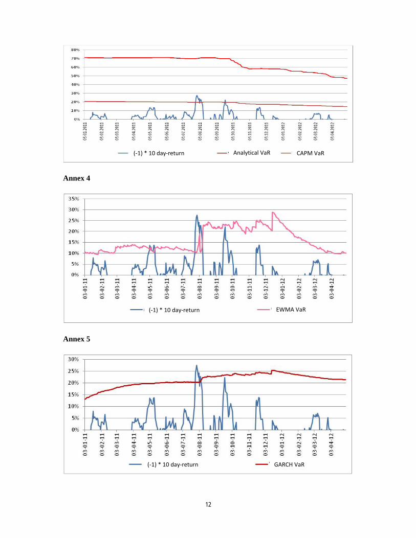
EWMA VaR was computed using a coefficient of persistence of the volatility of 0.95 ( .

Using the past volatility and returns, the updated volatility was determined and consequently

the EWMA VaR. In early 2011, the measure tends to overestimate risk VaR because of

volatility persistence, causing the EWMA to retain the past high volatility, but compared to

the Historical VaR the "ghost" effect is not so significant. After mid-2011 we can see that

VaR remains at the same levels due to the low inherited volatility, thus it follows a trend

closer to the 10 days losses of the portfolio, but does not react quickly enough to market

changes; only starting from the end of 2011 it incorporates these changes. These observations

are drawn from the results presented in Annex 4.

For computing GARCH VaR, a GARCH model was built for the portfolio returns. The

coefficient obtained for the persistence of volatility ( was 0.98 and the coefficient of the

6

unexpected return ( was 0.01. Out of the VaR measures outlined above, GARCH VaR most

closely follows the 10 days losses of the portfolio as illustrated in Annex 5. Consequently it

does not underestimate or overestimate consistently the market risk; this happens even at the

end of 2011, a period during which other VaR measures have not correctly anticipated

maximum potential loss. The choice of the volatility persistence coefficient is not made

arbitrarily as in the case of EWMA VaR, but by estimating the parameters based on the in-

sample period, this is why GARCH VaR is more accurate than the EWMA VaR.

In order to generate the price paths required by the Monte Carlo VaR, the previous GARCH

model was used for obtaining the conditional volatility for each scenario. Using the 10 day-

forecasted volatility obtained by using the GARCH model and the random generated number,

the 10,000 simulated returns were obtained. By computing the 1% percentile of the

distributions of 10 days returns, the results in Annex 6 were obtained. This model most

accurately assesses the market risk, eliminating the disadvantages of the previous methods,

being a forward looking model.

The first step in back-testing of the models was to determine the Rate of Failure (the ratio of

exceptions out of the total number of observations). The results obtained were the following:

Historical VaR (0%), Monte Carlo VaR (0.39%), GARCH VaR (2.14%), Analytic VaR

(3.36%), CAPM VaR (2.75%), EWMA VaR (4.28%). The second step was to test the

conditional coverage property, thus including the independence property. By comparing

with the 1% percentile of the distribution with one degree of freedom

(6.6349), as expected during the in-sample period, the VaR measures that didn’t pass the test

were EWMA VaR and CAPM VaR; during the out-of-sample period these measures were

accompanied by the Analytical VaR. It is worth mentioning that the only VaR measure that

passed the conditional coverage test, thus both the test of independence, was Monte Carlo

VaR, Historical VaR passed the independence test but not the unconditional coverage test.

CVaR models characteristics and back-testing results

For each of the VaR models, CVaR was computed by computing the surface of the area under

the distribution of returns which was bounded to the right by the VaR value. As expected by

construction, all CVaR models provided higher values than the VaR models.

7

Risk measured through CVaR reflected the market risk better, including during the periods in

which major losses were incurred. The performance of CVaR models depends on the method

used for computing VaR, for example Historical and Analytical CVaR overestimate the risk,

but changing the number of observations taken into account from 748 to 250 for these two

models, the results are improved.

The results of the CVaR models are consistently better for each method than those obtained

through VaR models; this is due to the fact that the average losses incorporate also the values

higher than VaR for each model. The results are presented in Annex 7, Annex 8 and Annex 9.

5 Results of the second challenge

Having the confirmation from the previous challenge that VAR and CVaR models through

Monte Carlo simulations are the best models for measuring market risk, the risk of BET-FI

was quantified by implementing these two models, the results obtained are presented in the

Annex 9, Annex 10 and Annex 11.

As can be seen in the Annex 11, the risk for the portfolio in 2011 and 2012 is lower than that

of BET-FI, except during the period July-August 2011; on an overall basis the risk of the

portfolio is less in 64% of cases than that of the BET-FI index. The average CVaR is in all

years higher for BET-FI than for the Portfolio, while the returns of BET-FI are lower in all

years (except in 2008 when the portfolio and BET-FI have both a return of -83%).

In order to assess the trade-off between risk and return, Sharpe and Treynor ratio, as well as

and Jensen’s Alpha were computed. Taking into account the limits of these indicators

when returns are negative, we made the comparison between BET-FI index portfolio only for

the years 2009 and 2012. The Portfolio presented a superior trade-off between risk and returns

in both years. Nevertheless, we must bear in mind the disadvantages of using the standard

deviation (used in the above mentioned indicators) as a measure of market risk. Moreover, by

computing the Tracking Error and analyzing the values for the Information Ratio, it can be

easily observed that the performance of the Portfolio is consistent with an enhanced tracking

index strategy.

6 Results of the third challenge

8

To reduce the risk of the Portfolio, European put options with one year maturity on the BET-

FI were bought. For every year a new number of put options with different strike prices were

acquired. The number of puts chosen was based on a Protective Put strategy and the exercise

price was chosen to make the option be at the money in case of the last year’s scenario. The

characteristics of the options are presented in Annex 14. The risk and return of the hedged and

unhedged Portfolio are shown in Annex 13 and Annex 15.

In 2011, when the BET-FI decreased by 15%, the use of options was reflected not only in the

reduction of the average risk with 4% (measured as Monte Carlo CVaR), but ensured a higher

return, even if a negative one (-6%) compared with the return of the unprotected portfolio

return (-10%).

In 2012, the Average CVaR for the protected Portfolio was 7% lower than that of the

unprotected Portfolio, justifying clearly in terms of the risk analysis the usage of options.

Comparing the effects of using options, it can be observed that the risk of the unprotected

Portfolio is higher in 99.86% of cases. In 2012, the risk mitigation was reflected in a return of

only 19% compared with the 24% of the unhedged Portfolio. This difference came from

purchasing options that were not exercised, while the premium paid for them was quite high

due to high levels of volatility.

7 Conclusions

In very volatile conditions, the market risk assessment becomes very important because the

portfolio losses can be significant and very difficult to anticipate. Knowing the maximum

level of losses over a short period of time (10 days) with a confidence level (99%) makes it

easier to understand the consequences of being exposed to market risk. The best model that

fulfils the unconditional coverage and independence property is Monte Carlo VaR. When

computing CVaR the performance of all the models is improved, but the ranking between

them remains the same. Using a fundamentally weighted Portfolio of shares a lower risk and a

higher return (with only one exception - year 2008) is obtained vis-à-vis the BET-FI indes

which is weighted depending on the market capitalization. Using a Protective Put strategy the

hedged portfolio reduced its risk, while the impact on returns is asymmetrical, the returns are

lower in 2012 and higher in 2011 than those of the unhedged portfolio.

9

Bibliography

[1] Alexander, C 2008, Market risk analysis - Practical financial econometrics, John Wiley

& Sons, West Sussex.

[2] Alexander, C 2009, Market risk analysis - Value-at-risk models, John Wiley & Sons,

West Sussex.

[3] Barone-Adesi, G, Bourgoin, F & Giannopoulos, K 1999, ‘Don’t Look Back’, Risk, nr.11,

p 100-104.

[4] Bodie, Z, Kane, A & Marcus, AJ 2007, Investments, the 7th edition, McGraw-Hill

Primis, New York.

[5] Bollerslev, T, Chou, RY & Kroner, KF 1992, ‘ARCH Modeling in Finance: A Selective

Review of the Theory and Empirical Evidence‘, Journal of Econometrics, vol. 52, p 5-59.

[6] Boudoukh, J, Richardson, M & Whitelaw, R 1998, ‘The Best of Both Worlds‘, Risk,

no.11, p 64-67.

[7] Brooks, C 2002, Introductory Econometrics for Finance, Cambridge University Press,

Cambridge.

[8] Campbell, JY, Lo, WA & MacKinlay, AC 1997, The Econometrics of Financial Markets,

Princeton University Press, New Jersey.

[9] Campbell, SD 2007, ‘A Review of Backtesting and Backtesting Procedures’, Journal of

Risk, vol. 9, Winter 2007, p 1-17.

[10] Christoffersen, P & Pelletier, D 2004, ‘Backtesting Value-at-Risk: A Duration-Based

Approach’, Journal of Empirical Finance, no.2, p 84-108.

[11] Codirla�u, AD & Chide�ciuc, NA 2008, Econometrie aplicată utilizând Eviews 5,

visited on 10 March 2012, <http://www.dofin.ase.ro/acodirlasu/

/econometriebancara2008.pdf>.

[12] Glasserman, P 2003, Monte Carlo Methods in Financial Engineering, Springer-Verlag,

New York.

[13] Graham, B 1949, The Intelligent Investor: The Definitive Book on Value Investing,

Collins Business, New York.

[14] Greene, WH 2003, Econometric analysis, a V-a edi�ie, Prentice Hall, New Jersey.

[15] Holton, AG 2003, Value-at-risk : theory and practice, Academic Press, Londra.

10

[16] Hull, JC 2002, Options, Futures and other derivatives, The 5th edition, Prentice Hall,

New Jersey.

[17] J. P. Morgan&Reuters 1996, RiskMetrics – Technical Document, The 4th edition, Morgan

Guaranty Trust Company, New York.

[18] Kuester, K, Mittnik, S & Paolella, 2006, ‘Value–at–Risk Prediction: A Comparison of

Alternative Strategies’, Journal of Financial Econometrics, vol.4, no. 1, p 53-89.

[19] Kupiec, P 1995, ‘Techniques for Verifying the Accuracy of Risk Management Models’,

Journal of Derivatives, no.3, p 73-84.

[20] Mishkin, FS 2003, The economics of Money, Banking and Financial Markets, the 7th

edition, Addison Wesley, San Francisco.

[21] Necula, C 2009, Evaluarea op�iunilor financiare. Volumul I - Modelul Black-Scholes-

Merton, Editura ASE, Bucure�ti.

[22] Ozerturk, S 2008, ‘Hedging with an index option’, visited on 1st June 2012,

<http://faculty.smu.edu/ozerturk/4378pdf/lecture9.pdf>.

[23] Powell R.J., Allen D.E, 2007, ‘Thoughts on VaR and CVaR’, Modelling and Simulation

Society of Australia and New Zealand

[24] Poonn, SH 2005, A Practical Guide to Forecasting Financial Market Volatility, I ediţie,

John Wiley & Sons, West Sussex.

[25] Sühan Altay, C. Coşkun Küçüközmen, 2009, ‘An assessment of value-at risk (VaR) and

expected tail loss (ETL) under a stress testing framework for Turkish stock market’, The

Journal of Risk Finance, vol. 11, p 164-179

[26] Yong Bao, Tae-Hwy Lee, Burak Saltoglu, 2006, ‘Evaluating Predictive Performance of

Value-at-Risk Models in Emerging Markets: A Reality Check’, The Journal of

Forecasting, no. 25, p 101-128

11

Annex 1

Annex 2

Annex 3

(‐1) * 10 day‐return Historical VaR 

(‐1) * 10 day‐return Analytical VaR 

12

Annex 4

Annex 5

(‐1) * 10 day‐return Analytical VaR CAPM VaR 

EWMA VaR (‐1) * 10 day‐return

(‐1) * 10 day‐return GARCH VaR 

13

Annex 6

Annex 7

Annex 8

Annex 9

(‐1) * 10 day‐return

(‐1) * 10 day‐returnMonte Carlo VaR

Analytical VaR Analytical CVaR

(‐1) * 10 day‐return Historical VaR Historical CVaR

14

Annex 10

Annex 11

Annex 12

(‐1) * 10 day‐return Monte Carlo CVaRMonte Carlo VaR 

Monte Carlo CVaRMonte Carlo VaR(‐1) * 10 day‐return

Monte Carlo CVaR Portfolio Monte Carlo CVaR BET‐FI

15

Portofolio BET-FI Year Return Average CVaR Return Average CvaR

2008 -83% 35% -83% 38% 2009 99% 39% 90% 42% 2010 -9% 29% -10% 34% 2011 -10% 27% -15% 27% 2012 24% 21% 22% 26%

Annex 13

Annex 14

Year BET-FI before

buying the option K

No. of puts

Cost of puts Value of puts at

expiration

2011 28,688 31,909 1.04 5,626. 47

RON 7,039.76 RON

2012 25,140 24,281 1.10 1,517.79 RON 1. 517,79 RON

Annex 15

Year Return of hedged

Portfolio Average CvaR

hedged Portfolio

Average CvaR unhedged Portfolio

Return of unhedged Portfolio

2011 -6% 22% 27% -10%

Monte Carlo CVaR Portfolio Monte Carlo CVaR Hedged Portfolio

16

2012 19% 14% 21% 24%